Measurement of ionization quenching in plastic scintillators

Abstract

Plastic scintillators are widely used in high-energy and medical physics, often for measuring the energy of ionizing radiation. Their main disadvantage is their non-linear response to highly ionizing radiation, called ionization quenching. This nonlinearity must be modeled and corrected for in applications where an accurate energy measurement is required. We present a new experimental technique to granularly measure the dependence of quenching on energy-deposition density. Based on this method, we determine the parameters for four commonly used quenching models for two commonly used plastic scintillators using protons with energies of $30\text{\,}\mathrm{M}\mathrm{e}\mathrm{V}$ to $100\text{\,}\mathrm{M}\mathrm{e}\mathrm{V}$; and compare the models using a Bayesian approach. We also report the first model-independent measurement of the dependence of ionization quenching on energy-deposition density, providing a purely empirical view into quenching.

1 Introduction

Plastic scintillators are widely used in particle detectors in high-energy physics experiments and for medical applications, for example in radiotherapy [1, 2]. When a charged particle passes through a scintillator, it loses energy by ionizing scintillator molecules, leaving them in excited states. These excited molecules can emit light when they relax, providing a measurable signal. Since the light yield is related to a particle’s energy loss, scintillators are used in calorimeters. Since scintillators are easily segmented, they are also used in particle trackers.

When the density of energy lost by a particle is low, a scintillator’s light yield is linearly proportional to the energy lost. When the density is high, the production of detectable light is hindered by various processes and the light yield is nonlinearly proportional to the energy lost [3]. This reduction is called ionization quenching [4].

At high momentum, a particle loses relatively little energy per distance in comparison to its kinetic energy; so its momentum decreases very slowly. The energy-loss rate is also only weakly dependent on the particle’s momentum; so the light yield per distance at high momentum is nearly constant and easily calibrated. This means scintillators produce consistent and reliable signals useful for tracking high-energy particles.

Additionally, if a particle is stopped (or significantly slowed) within a scintillator, the light produced can be used to measure the particle’s energy. But at low momentum, a particle loses large amounts of energy over short distances, so ionization quenching significantly reduces the light emission and complicates the energy measurement. Accurate calorimetry of highly ionizing radiation requires a good understanding of quenching.

The magnitude of quenching is dependent on the amount of energy deposited in a scintillator per unit distance. Many competing models parametrize this dependence via quenching functions [3, 5, 6, 7, 8]. Most of these functions are based on assumptions about discrete interactions of particles with scintillator molecules and of excited scintillator molecules with each other. But none are capable of predicting the values of their parameters—they are empirical.

Using data collected with two widely-used plastic scintillators, we determine the parameters for four quenching models [3, 5, 7, 8]. Using Bayesian statistics, we compare the probabilities for the models to explain our data. We also fit a model-independent quenching function to our data to learn about the dependence of quenching on energy deposition free from assumptions. We compare this result to those of the four models we tested and discuss their advantages and deficiencies. To our knowledge, this is the first direct measurement of a quenching function without modeling.

2 Quenching models

The response of a scintillating material to a charged particle is characterized by its light yield per unit of distance traveled by the particle, $\derivative*{L}{x}$. However, the light yield per unit of energy deposited by the particle over that distance, $\derivative*{L}{E}$, is more useful in modeling and simulation. The two are related to each other by

$$\derivative{L}{x}=\derivative{L}{E}\cdot\derivative{E}{x},$$ (1)

where $\derivative*{E}{x}$ is the energy lost by the particle per unit of distance, which depends on the energy of the particle (as well as its species and the scintillator material). To simplify our equations, we denote $\derivative*{E}{x}$, a function of the particle’s kinetic energy, $T$, as $\epsilon(T)$. The light yield per unit of energy deposited is a function of $\epsilon$, and therefore indirectly of $T$:

$$\evaluated{\derivative{L}{E}}_{T}\equiv S\cdot Q\quantity(\epsilon(T)),$$ (2)

where $Q(\epsilon)$ is the unitless quenching function, defined such that at small $\epsilon$ (that is, at high kinetic energy), it goes to unity; $S$ is the linear proportionality of light yield to energy deposition at high energy and has units of photons per energy. So the light yield per unit of distance is

$$\evaluated{\derivative{L}{x}}_{T}=\epsilon(T)\cdot S\cdot Q\quantity(\epsilon(T)).$$ (3)

Scintillation light is produced via several steps [3]: a passing particle ionizes molecules of the scintillator’s base plastic material, which then emit light. In a pure plastic, this light is quickly reabsorbed by other molecules. To allow the light to propagate further, the plastic is doped with a molecule that absorbs this light and emits light of a shifted wavelength. Since neither the base molecule nor the dopant efficiently absorbs the wave-length-shifted light, it propagates long distances. However, dopant molecules can absorb photons without re-emitting them or can re-emit them at wavelengths unsuitable for detection. This occurs when they have been excited by interaction with the ionizing particle.

J. B. Birks developed the first model of ionization quenching in the early 1950s, which is still widely used [3]. He parametrized quenching in terms of the density of excited dopant molecules, $B$, and the probability for non-radiative relaxation, $k$:

$$Q_{\text{Birks}}(\epsilon)=1/(1+kB\,\epsilon).$$ (4)

Since $k$ and $B$ appear only as a product, they act as one parameter, $kB$, called Birks’ coefficient, which has units of distance per energy. Its value depends on the scintillating material.

Many authors have extended Birks’ model: Chou et al. accounted for secondary effects by adding a term to the denominator that is second order in $\epsilon$:

$$Q_{\text{Chou}}(\epsilon)=1/(1+kB\,\epsilon+C\epsilon^{2}),$$ (5)

where $\sqrt{C}$ has the same units as $kB$ [5, 6]. Wright et al. defined the phenomenological quenching function

$$Q_{\text{Wright}}(\epsilon)\equiv\frac{1}{W\epsilon}\log(1+W\epsilon),$$ (6)

where $W$ has the same units as $kB$ [7]. Voltz et al. developed the first model to distinguish between primary and secondary ionization: The primary particle can produce high-energy electrons as it ionizes the scintillator molecules. They travel away from the path of the primary particle, losing energy via ionization of the scintillator and spreading out the energy deposition, which weakens quenching. The Voltz model assumes that a fraction of deposited energy, $f$, is unquenched and parametrizes the quenching of the remaining fraction with an exponential function:

$$Q_{\text{Voltz}}(\epsilon)\equiv f+(1-f)e^{-V(1-f)\epsilon},$$ (7)

where $V$ has the same units as $kB$ [8].

Like Birks’ coefficient, $C$, $W$, and $V$ all depend on the scintillator material. All four must be positive and are independent of the species of the particle interacting with the scintillator. The Voltz model’s $f$ depends on both the scintillator material and primary particle species [9]. None of the parameters can be predicted from first principles—all must be measured experimentally.

These quenching functions have some common features: As we require of a quenching function, they are all bounded by 1 above, which is approached as $\epsilon\to 0$; and by 0 below, which may be approached as $\epsilon\to\infty$. All have negative first derivatives ($\derivative*{Q}{\epsilon}$) everywhere regardless of their parameters and therefore always monotonically decrease. Birks’, Wright’s, and Voltz’ functions all have positive second derivatives everywhere regardless of their parameter values; only Chou’s function allows for a negative second derivative and a potential inflection point. These properties will be important when we compare model-dependent and model-independent results.

3 Quenching measurement

To determine each model’s parameters and which model most accurately describes quenching, we measure $\derivative*{L}{E}$ at several kinetic energies and fit the parameterizations of $Q(\epsilon)$ to this data using equation (2).

Many issues complicate this task: We cannot directly measure $\derivative*{L}{E}$; instead we measure the amount of light, $L$, produced by a particle that has lost energy in the scintillator. So we must integrate equation (2):

$$L(T^{\text{in}},T^{\text{out}})=S\!\int\limits_{\mathrlap{T^{\text{out}}}}^{\mathrlap{T^{\text{in}}}}\!Q\quantity(\epsilon(T))\,\differential{T},$$ (8)

where $T^{\text{in}}$ and $T^{\text{out}}$ are the incoming and outgoing kinetic energies of the particle. $Q$ is not directly a function of $T$, but instead of $\epsilon(T)$, which is a stochastic function: At a particular kinetic energy, we know the mean energy loss per unit distance for particles with that energy from both the Bethe formula and experiment [10, 11]. But an individual particle’s energy loss stochastically deviates from the mean according to distributions whose shapes are also $T$ dependent [11, 12, 13]. This stochastic behavior is difficult and computationally expensive to model. So instead of studying the behavior of individual particles, we study the behavior of an ensemble of particles. We measure the distribution of $L(T^{\text{in}},T^{\text{out}})$ and fit the quenching model parameters to the mean amount of light, $\bar{L}$, produced by an ensemble of particles given a mean energy loss, $\bar{\epsilon}$:

$$\bar{L}(\bar{T}^{\text{in}},\bar{T}^{\text{out}})=S\!\int\limits_{\mathrlap{\bar{T}^{\text{out}}}}^{\mathrlap{\bar{T}^{\text{in}}}}\!\bar{Q}\quantity(\bar{\epsilon}(T))\,\differential{T},$$ (9)

where $\bar{T}^{\text{in}}$ and $\bar{T}^{\text{out}}$ are the mean incoming and outgoing kinetic energies of the ensemble and $\bar{Q}$ is the quenching function of the mean energy of an ensemble. We assume quenching of the mean energy loss is described identically to quenching of the stochastic energy loss: $\bar{Q}=Q$.

The above equations are further complicated by how the scintillation light is measured: it propagates through the scintillator to a light detector. Both propagation and detection cause losses of light. In our experimental setup, these losses linearly scale the light yield and can be canceled out by measuring with respect to a reference light yield. To simplify our calculations, we measure with respect to the signal produced by a particle with $\epsilon x\ll T$ for distances, $x$, even much larger than our setup. To very good approximation, the light yield of such a particle is

$$\bar{L}_{\text{ref}}=S\!\int\limits_{\mathrlap{\bar{T}-\epsilon_{\text{ref}}\bar{x}}}^{\mathrlap{\bar{T}}}\!\bar{Q}\quantity(\bar{\epsilon}(T))\,\differential{T}\approx\bar{\epsilon}_{\text{ref}}\,\bar{x}\,S\,\bar{Q}(\bar{\epsilon}_{\text{ref}}),$$ (10)

where $\bar{\epsilon}_{\text{ref}}$ is the mean energy loss per unit distance of the reference particle and $\bar{x}$ is the mean length of scintillator passed through. We define the relative mean light yield as

$$\bar{\Lambda}(\bar{T}^{\text{in}},\bar{T}^{\text{out}})\equiv\frac{\bar{L}(\bar{T}^{\text{in}},\bar{T}^{\text{out}})}{\bar{L}_{\text{ref}}}=\frac{1}{\bar{\epsilon}_{\text{ref}}\,\bar{x}\,\bar{Q}\quantity(\bar{\epsilon}_{\text{ref}})}\,\int\limits_{\mathrlap{\bar{T}^{\text{out}}}}^{\mathrlap{\bar{T}^{\text{in}}}}\!\bar{Q}\quantity(\bar{\epsilon}(T))\,\differential{T.}$$ (11)

To gather granular data for a range of $\bar{\epsilon}$, we use a segmented detector consisting of an array of scintillating fibers laid in a row. We shoot a beam of protons and pions into the detector such that pions could traverse all fibers successively and protons could stop within the array. We vary the energies of the beams and the angle of incidence on the fibers, $\theta$, which changes $\bar{x}$. The protons serve as test particles for measuring quenching, and the pions serve as the low-$\epsilon$ reference particles for the relative light yield measurement. From initial kinetic energies in the range of tens to hundreds of $\mathrm{M}\mathrm{e}\mathrm{V}$ to stopping, the range of $\bar{\epsilon}$ for the protons varies by two orders of magnitude, while the through-going pions are always in their minimum-ionizing energy range, regardless of incoming beam energy. Though changes of the angle only translate into small changes of the protons’ path lengths in the fibers, they strongly affect their energy-loss profiles because of the high stopping power of protons shortly before stopping. Where the energy loss is largest, quenching effects are most pronounced; so small variations of the angle lead to large variations in quenching and significantly improve our measurement sensitivity. We label each different setting of beam energy and incidence angle as a run.

In each run, we measure $\bar{\Lambda}_{i}$ for each fiber, with $i$ labeling the fiber; this is the data set for each run. Unfortunately we do not know $\bar{T}^{\text{in}}_{i}$ and $\bar{T}^{\text{out}}_{i}$ for individual fibers. In our fits to the $\bar{\Lambda}_{i}$, the mean energy of the proton beam prior to it entering the fiber array, $\bar{T}_{0}$ is a free parameter. We calculate all the incoming and outgoing energies, $\bar{T}^{\text{in}}_{i}$ and $\bar{T}^{\text{out}}_{i}$ ($i\geq 1$), with the continuous-slowing-down approximation (CSDA) using data from the National Institute of Standards and Technology (NIST) for $\bar{\epsilon}(T)$ [14, 15]. We account for inactive coatings on the fibers, so $\bar{T}_{0}\neq\bar{T}^{\text{in}}_{1}$ and $\bar{T}^{\text{out}}_{i}\neq\bar{T}^{\text{in}}_{i+1}$. This calculation depends on $\bar{x}$, and therefore on the incidence angle, which is also a free parameter in our fits.

3.1 Fit likelihood

To fit a quenching model, $M$, to our data, we must quantify how well it describes the data given particular values of its parameters, $\vec{\lambda}$. This is the likelihood of the data given the model and its parameters. Since the likelihood for the data of an individual run has a common form for all runs, we factorize the likelihood to describe our total data set, $\vec{D}$, into the product of likelihoods to describe the data of individual runs, $\vec{D}_{r}$:

$$\mathcal{L}(\vec{D}\,|\,\vec{\lambda},\vec{\nu};M)\equiv\prod_{r}\mathcal{L}_{r}(\vec{D}_{r}\,|\,\vec{\lambda},\vec{\nu}_{r};M),$$ (12)

where $\vec{\nu}$ is the vector of beam parameters vectors, $\vec{\nu}_{r}=\{\bar{T}_{r0},\theta_{r}\}$, for all runs; and the data for a particular run, $\vec{D}_{r}$, are the observed $\bar{\Lambda}_{ri}^{\text{obs}}$ and their uncertainties, $\sigma_{ri}$. The likelihood for an individual run is

$$\mathcal{L}_{r}(\vec{D}_{r}\,|\,\vec{\lambda},\vec{\nu}_{r};M)\equiv\prod_{i}\mathcal{N}\quantity(\bar{\Lambda}_{i}^{\text{exp}}(\vec{\lambda},\vec{\nu}_{r};M)\,|\,\bar{\Lambda}_{ri}^{\text{obs}},\sigma_{ri}),$$ (13)

where $\mathcal{N}$ is the normal distribution and $\bar{\Lambda}_{i}^{\text{exp}}$ is the expectation for the quenched mean relative light yield calculated according to equation (11) using quenching model $M$.

To calculate $\bar{\Lambda}_{i}^{\text{exp}}$, we first simulate the trajectory of a particle with an initial energy $\bar{T}_{r0}$ and incidence angle $\theta_{r}$ through the fiber array, calculating its energy losses in both the active and inactive layers of the array with NIST’s CSDA data. From the simulation we know the integration limits of equation (11). To account for the variation in the pion momentum from run to run, we replace $\bar{\epsilon}_{\text{ref}}$ in equation (11), with a run-dependent mean pion energy-loss density, $\bar{\epsilon}^{\!\;\mathup{{{\pi}}}}_{r}$. The mean distance traversed by a pion in a fiber is calculated from the incidence angle for the run: $\bar{x}=\ifrac{w}{\cos\theta_{r}}$, where $w$ is the width of the active layer of a fiber. To emphasize the parameter dependence, we rewrite equation (11) explicitly for this context:

$$\bar{\Lambda}_{i}^{\text{exp}}(\vec{\lambda},\vec{\nu}_{r};M)=\frac{\cos\theta_{r}}{\bar{\epsilon}^{\!\;\mathup{{{\pi}}}}_{r}w\;\bar{Q}_{M}(\bar{\epsilon}^{\!\;\mathup{{{\pi}}}}_{r}\!;\vec{\lambda})}\;\int\limits_{\mathrlap{\bar{T}^{\text{out}}_{i}(T_{r0},\theta_{r})}}^{\mathrlap{\bar{T}^{\text{in}}_{i}(T_{r0},\theta_{r})}}\!\bar{Q}_{M}\quantity(\bar{\epsilon}(T);\vec{\lambda})\differential{T},$$ (14)

where now $\vec{\nu}_{r}=\{\bar{T}_{r0},\theta_{r},\bar{\epsilon}^{\!\;\mathup{{{\pi}}}}_{r}\}$.

Runs with different angles were taken at common beam momenta; and runs with different beam momenta were taken at common angles. Runs with a common beam momentum share a single $T_{r0}$ and a single $\bar{\epsilon}^{\,\mathup{{{\pi}}}}_{r}$; and runs with a common angle share a single $\theta_{r}$.

We explore the parameter space of each model using a Bayesian formulation of probability and a Markov-Chain Monte-Carlo (MCMC) algorithm implemented by the Bayesian Analysis Toolkit [16, 17, 18]. This defines the posterior probability—the probability for parameters given our knowledge after the experiment—as the product of the above likelihood and a prior probability:

$$P(\vec{\lambda},\vec{\nu}\,|\,\vec{D};M)\propto\mathcal{L}(\vec{D}\,|\,\vec{\lambda},\vec{\nu};M)\times P_{0}(\vec{\lambda},\vec{\nu}\,|\,M),$$ (15)

where proportionality is used since the right-hand side must be normalized for the product to be a probability. The prior probability, $P_{0}$, of parameters reflects our knowledge before the experiment. For each model and for each scintillator type, we fit the parameters to all data sets simultaneously. The free parameters in each fit are all $T_{r0}$, $\theta_{r}$, and $\bar{\epsilon}^{\!\;\mathup{{{\pi}}}}_{r}$ and the parameters of the quenching model studied.

This approach necessitates that we choose a prior probability distribution for all parameters. Although we have precise knowledge of the proton and pion energies in the beam, we use informative uniform prior probability distributions for the $T_{r0}$ and $\bar{\epsilon}^{\!\;\mathup{{{\pi}}}}_{r}$. We do this since the beam passes through two windows and a short gap of air before entering the detector array. Interaction with the windows and air smears out the energy distribution. The prior for each $\theta_{r}$ is a normal distribution with mean and standard deviation learned from an independent fit to pion data that calibrates the experiment’s rotatory table. The priors for the model parameters are discussed below alongside the fit results.

The NIST data used to calculate the $\bar{\Lambda}^{\text{exp}}$ has an uncertainty that scales the entire stopping-power data set up or down together, not affecting the $T$ dependence of $\bar{\epsilon}$. We account for this uncertainty with a parameter that scales the CSDA data. It has a normal prior probability distribution centered at unity with a standard deviation of $4\text{\,}\mathrm{\char 37\relax}$—the known uncertainty from NIST. This parameter is also free in the fit, but its posterior probability is identical to its prior probability. Though this uncertainty affects all analyses that rely on NIST data, it has been neglected in most existing measurements.

3.2 Model comparison

We compare models to each other by calculating Bayes factors, which quantify the relative abilities of two models to describe the data regardless of the best-fit values found for their parameters [19]. This approach accounts for model complexities, full posterior probability distributions, and overfitting (acting as an Occam’s razor).

The Bayes factor, $K_{\text{AB}}$, comparing model A to model B, is the ratio of the model evidences, $z_{\text{A}}$ and $z_{\text{B}}$,

$$K_{\text{AB}}\equiv\frac{z_{\text{A}}}{z_{\text{B}}}.$$ (16)

The evidence of a model is a measure of its ability to describe the data regardless of the values of its parameters. It is the integral over the right-hand side of equation 15

$$z_{M}=\int\!\mathcal{L}(\vec{D}\,|\,\vec{\lambda},\vec{\nu};M)\,P_{0}(\vec{\lambda},\vec{\nu}\,|\,M)\,\differential\vec{\lambda}\,\differential\vec{\nu},$$ (17)

—the integrand is the product of the likelihood and the prior probability density and the integration is over all parameters and over the entirety of each parameter’s allowed range.

The posterior belief in preferring model A over model B is

$$\frac{P(\text{A})}{P(\text{B})}=K_{\text{AB}}\cdot\frac{P_{0}(\text{A})}{P_{0}(\text{B})},$$ (18)

where $P_{0}(M)$ and $P(M)$ are the prior and posterior probabilities for a particular model—that is, one’s belief in the model before and after the experiment. The prior probabilities, $P_{0}(A)$ and $P_{0}(B)$, are subjectively chosen by each scientist. The Bayes factor thus quantifies the objective part of our learning process and separates it from the subjective priors. If $K_{\text{AB}}$ is greater than one, model A is preferred over model B by the data; if $K_{\text{AB}}$ is less than one, model B is preferred over model A by the data.

The integral in equation (17) is not generally easy to calculate. We used a harmonic-mean estimator (HME) algorithm to calculate evidences from the MCMC samples [20]. We calculate the evidence from the samples by

$$z_{\text{M}}\approx\quantity(\frac{1}{N}\sum_{i=1}^{N}\frac{1}{\mathcal{L}(\vec{D}\,|\,\vec{\lambda}_{i},\vec{\nu}_{i};M)\,P_{0}(\vec{\lambda}_{i},\vec{\nu}_{i}\,|\,M)})^{\!\!\!-1},$$ (19)

where the sum is over the $N$ sampled parameter points in the Markov chain. Since this method suffers from numerical instabilities in regions of small posterior probability density, we restricted our evaluation of the HME to a volume in which the calculation is well behaved and accounted for this restriction in calculating the evidence using an algorithm developed in [21].

4 Experimental setup

diagram

Figure 1: Schematic of the experimental setup.

Our detector consists of 16 scintillating fibers, each $71\text{\,}\mathrm{m}\mathrm{m}$ long with a square $$2\text{\,}\mathrm{m}\mathrm{m}$\times$2\text{\,}\mathrm{m}\mathrm{m}$$ cross section. We arrange them such that their long sides were perpendicular to the beam and place them in a row such that the beam passed through them sequentially. Figure 1 shows a schematic view of the experimental setup. We measured with two different scintillating materials: SCSF-78 from Kuraray, with a polystyrene base; and BC-408 from Saint-Gobain, with a polyvinyltoluene base [22, 23].

The light produced in each fiber is detected by a square $$3\text{\,}\mathrm{m}\mathrm{m}$\times$3\text{\,}\mathrm{m}\mathrm{m}$$ Hamamatsu Photonics S13360-4935 silicon photomultiplier (SiPM) glued to one end of the fiber [24]. Each SiPM has a pitch size of $25\text{\,}\mathrm{\SIUnitSymbolMicro}\mathrm{m}$ with $14\,400$ pixels in total, of which $6400\text{\,}\mathrm{o}$verlap with the fiber end. The large SiPM eases the gluing process and minimizes variations due to positioning errors. The measurements were performed with constant overvoltages on the SiPMs and constant temperatures to ensure consistent gains throughout measuring. From simulation, we estimate an average SiPM signal of 10 to 15 photoelectrons for a pion and around 200 photoelectrons for the maximum signal from a proton. So saturation effects are negligible and we have constant light detection efficiency for both the pions and the protons [25]. From test measurements in which we varied the vertical position of the detector relative to the beam, we observed no dependence of our measurements on this alignment. To digitize the SiPM signals, we use multichannel mezzanine-sampling analog-to-digital converters (ADCs) [26].

We measured in the $\mathup{{{\pi}}}$M1 beamline of the high-intensity proton accelerator at the Paul Scherrer Institute [27]. The $\mathup{{{\pi}}}$M1 beam consists of protons and pions with momenta adjustable between $220\text{\,}\mathrm{M}\mathrm{e}\mathrm{V}\mathrm{/}\mathrm{c}$ and $450\text{\,}\mathrm{M}\mathrm{e}\mathrm{V}\mathrm{/}\mathrm{c}$ with a resolution of about $1\text{\,}\mathrm{\char 37\relax}$ [28]. The beam spot size was $$10\text{\,}\mathrm{m}\mathrm{m}$\times$10\text{\,}\mathrm{m}\mathrm{m}$$ (at fwhm) and centered on the middle of our fibers. To reduce the beam divergence, we placed a copper collimator with a $2\text{\,}\mathrm{m}\mathrm{m}$-diameter bore before the fiber array, with $20\text{\,}\mathrm{c}\mathrm{m}$ between the exit of the collimator and the first fiber (at perpendicular incidence). The collimator produced a strongly collimated beam of protons that hit the center of the fiber array (at perpendicular incidence), but did not significantly alter the pion beam. The fiber array was mounted on a rotary table that allowed us to vary the angle of incidence of the beam on the array. The entire setup was placed in a vacuum chamber to minimize beam interactions with air before entering the detector.

The recorded data set for the SCSF-78 scintillator contains seven runs: five with an incidence angle of $1.6\text{\,}\mathrm{\SIUnitSymbolDegree}$ at momenta of $230\text{\,}\mathrm{M}\mathrm{e}\mathrm{V}\mathrm{/}\mathrm{c}$, $240\text{\,}\mathrm{M}\mathrm{e}\mathrm{V}\mathrm{/}\mathrm{c}$, $275\text{\,}\mathrm{M}\mathrm{e}\mathrm{V}\mathrm{/}\mathrm{c}$, $300\text{\,}\mathrm{M}\mathrm{e}\mathrm{V}\mathrm{/}\mathrm{c}$, and $335\text{\,}\mathrm{M}\mathrm{e}\mathrm{V}\mathrm{/}\mathrm{c}$; and two further at $3.4\text{\,}\mathrm{\SIUnitSymbolDegree}$ and $8.4\text{\,}\mathrm{\SIUnitSymbolDegree}$, both at $335\text{\,}\mathrm{M}\mathrm{e}\mathrm{V}\mathrm{/}\mathrm{c}$. The recorded data set for the BC-408 scintillator contains six runs: four with an incidence angle of $1.6\text{\,}\mathrm{\SIUnitSymbolDegree}$ at momenta of $240\text{\,}\mathrm{M}\mathrm{e}\mathrm{V}\mathrm{/}\mathrm{c}$, $300\text{\,}\mathrm{M}\mathrm{e}\mathrm{V}\mathrm{/}\mathrm{c}$, $335\text{\,}\mathrm{M}\mathrm{e}\mathrm{V}\mathrm{/}\mathrm{c}$, and $350\text{\,}\mathrm{M}\mathrm{e}\mathrm{V}\mathrm{/}\mathrm{c}$; and two further at $5.4\text{\,}\mathrm{\SIUnitSymbolDegree}$ and $7.9\text{\,}\mathrm{\SIUnitSymbolDegree}$, both at $335\text{\,}\mathrm{M}\mathrm{e}\mathrm{V}\mathrm{/}\mathrm{c}$.

4.1 Relative light yield measurement

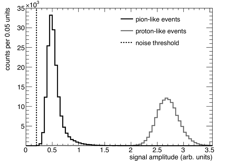
Figure 2: Pulse-height spectrum for the first fiber in the detector array for a beam momentum of $350\text{\,}\mathrm{M}\mathrm{e}\mathrm{V}\mathrm{/}\mathrm{c}$ and an incidence angle of $1.6\text{\,}\mathrm{\SIUnitSymbolDegree}$. The fiber type is SCSF-78.

In each run, the beam contains both protons and pions. An event consists of one particle passing through a contiguous part of the fiber array (always including the first fiber, which was used as a trigger), producing scintillation light in each traversed fiber. The SiPMs convert this light into charge signals, which are digitized in the ADCs. We fit to the ADC output to determine the signal amplitude for each fiber. Figure 2 shows the signal-amplitude spectrum for a single fiber and a single run.

At our beam momenta, pions pass through all 16 fibers with a nearly constant energy-loss density; accordingly we define an event as pion-like if it passes through all fibers. The signal in each fiber must be above the noise threshold measured for that fiber. Pion-like events form the low-amplitude peak in figure  2. The arithmetic mean of the spectral distribution of pion-like events is the uncalibrated mean pion light yield.

Since the minimum energy-loss density for a proton is three times higher than that for a pion, we define a proton-like event as one with more than one fiber with a signal amplitude exceeding three times the mean pion light yield for that fiber. Proton-like events form the high-amplitude peak in figure 2. The arithmetic mean of the spectral distribution of proton-like events is the uncalibrated mean proton light yield. The ratio of the uncalibrated mean proton light yield to the uncalibrated mean pion light yield is the relative mean light yield, $\bar{\Lambda}_{i}$.

The signals from the SiPMs are smeared by noise, the resolutions of the ADCs, the pulse-shape fits, and the event-selection algorithm. We estimate the uncertainty on the relative mean light yield from these effects by fitting a Landau distribution folded with a normal distribution to the pion peak in the signal-amplitude spectrum. We take the standard deviation of the normal distribution, $5\text{\,}\mathrm{\char 37\relax}$ (relative), as a conservative estimate of the measurement uncertainty on the mean light yield and add it (in quadrature) to the statistical uncertainty from the above steps. The result is the $\sigma_{ri}$ used in the likelihood for the model fit.

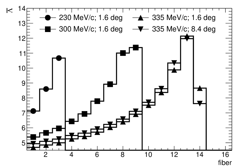
Figure 3: Relative mean light yield of proton-like events for four different runs measured with the SCSF-78 scintillator. The uncertainties are smaller than the symbols.

Figure 3 shows the relative mean light yield of five runs. For all four runs, we clearly see the Bragg curves for stopping particles, with the particle range increasing with increasing momentum. From the two runs at $335\text{\,}\mathrm{M}\mathrm{e}\mathrm{V}\mathrm{/}\mathrm{c}$, we see that changing the incidence angle causes measurable changes in the $\bar{\Lambda}$ profile.

5 Results

To evaluate each model’s posterior probability, we must choose prior probability distributions for the model’s parameters. We choose each prior to be uniform within a reasonable range, imposing physical constraints, and to be zero outside this range. All model parameters are constrained by requiring

$$0\leq\bar{Q}(\bar{\epsilon};\vec{\lambda})\leq 1\qquad\forall\,\bar{\epsilon}\geq 0.$$ (20)

This is fulfilled for all our models when their parameters are greater than or equal to zero. Additionally, for Voltz’ model, $f$ is bounded above by one.

model	par.	units	SCSF-78	corr.	BC-408	corr.
Birks	$kB$	$\mathrm{m}\mathrm{m}\mathrm{/}\mathrm{M}\mathrm{e}\mathrm{V}$	$0.132\pm 0.004$		$0.155\pm 0.005$
Chou	$kB$	$\mathrm{m}\mathrm{m}\mathrm{/}\mathrm{M}\mathrm{e}\mathrm{V}$	$0.000\leq 0.001^{\dagger}$	0.93	$0.151\pm 0.04$	0.75
	$\sqrt{C}$	$\mathrm{m}\mathrm{m}\mathrm{/}\mathrm{M}\mathrm{e}\mathrm{V}$	$0.129\pm 0.005$		$0.000\leq 0.002^{\dagger}$
Wright	$W$	$\mathrm{m}\mathrm{m}\mathrm{/}\mathrm{M}\mathrm{e}\mathrm{V}$	$0.333\pm 0.009$		$0.406\pm 0.002$
Voltz	$V$	$\mathrm{m}\mathrm{m}\mathrm{/}\mathrm{M}\mathrm{e}\mathrm{V}$	$0.091\pm 0.006$	0.25	$0.628\pm 0.108$	0.89
	$f$		$0.000\leq 0.057^{\dagger}$		$0.427\pm 0.019$

Table 1: Parameter values at the best-fit points, $68\text{\,}\mathrm{\char 37\relax}$-credibility-interval uncertainties, and the correlation factors (where applicable). ^†These best-fit values are at their boundaries, zero, so we give their $68\text{\,}\mathrm{\char 37\relax}$-credibility upper limits.

In table 1, for each of the four models and for each of the scintillating fiber types, we list the parameter points that maximize the posterior probability, which we refer to as the best-fit point; the $68\text{\,}\mathrm{\char 37\relax}$-credibility-interval uncertainties; and correlation factors (where applicable). The uncertainties and correlation factors include both statistical and systematic effects. We are able to measure Birks’ coefficient to a relative precision of $3\text{\,}\mathrm{\char 37\relax}$. Our value of Birks’ $kB$ for BC-408 agrees with that presented in [29].

We observe very different behavior of Chou’s model for the two scintillators: For SCSF-78, the term linear in $\bar{\epsilon}$ is negligible and quenching is best described by the quadratic term alone, with $\sqrt{C}$ compatible with Birks’ $kB$. For BC-408, the opposite is the case and quenching is best described by the linear term alone, with Chou’s $kB$ compatible with Birks’. Therefore Chou’s model requires the shape of the quenching function strongly depend on the scintillator material.

We also observe very different behavior of Voltz’ model for the two scintillators: For SCSF-78, $f$ is small, with a best-fit value of zero; Table 1 lists the mode and $68\text{\,}\mathrm{\char 37\relax}$-credibility upper limit. This means that all deposited energy is subject to quenching, as in Birks’ model. Accordingly, for this fiber type, $V$ is of a comparable scale to Birks’ $kB$. For BC-408, $f$ is closer to $50\text{\,}\mathrm{\char 37\relax}$—only half the deposited energy is subject to quenching. Accordingly, $V$ must be larger. This trend is confirmed by the positive correlation of the parameters in both fits with Voltz’ model. Voltz’ model also requires the shape of the quenching function strongly depend on the scintillator material.

5.1 Model-independent fit

$Q(\epsilon)$	998	996	962	922	856	629	419	405	309	113
$\epsilon$	5	10	15	20	30	50	75	100	250	500
5	$1.32$	$1.23$	$1.10$	$1.05$	$1.00$	$0.76$	$0.55$	$0.30$	$0.01$	$0.33$
10		$1.67$	$1.60$	$1.54$	$1.44$	$1.12$	$0.81$	$0.42$	$0.01$	$0.18$
15			$1.72$	$1.63$	$1.54$	$1.12$	$0.83$	$0.51$	$0.11$	$0.20$
20				$1.59$	$1.48$	$1.15$	$0.81$	$0.35$	$-0.16$	$0.04$
30					$1.44$	$0.99$	$0.81$	$0.41$	$-0.21$	$0.04$
50						$1.15$	$0.65$	$-0.40$	$-0.86$	$-0.65$
75							$1.94$	$-0.12$	$-1.51$	$-1.18$
100								$2.73$	$2.72$	$1.89$
250									10.8	$6.39$
500										10.2

Table 2: Result of model-independent fit to SCSF-78: $Q$ values (top) and covariances (bottom) in ‰ at fixed $\epsilon$ values (in $\mathrm{M}\mathrm{e}\mathrm{V}\mathrm{/}\mathrm{c}\mathrm{m}$).

$Q(\epsilon)$	989	847	768	709	652	517	444	412	263	115
$\epsilon$	5	10	15	20	30	50	75	100	250	500
5	$2.32$	$1.43$	$1.09$	$1.01$	$1.01$	$0.45$	$0.55$	$0.46$	$0.50$	$0.28$
10		$3.88$	$3.95$	$3.67$	$3.59$	$2.32$	$1.23$	$0.73$	$0.94$	$0.69$
15			$4.22$	$3.90$	$3.89$	$2.22$	$1.12$	$0.61$	$0.80$	$0.63$
20				$3.65$	$3.65$	$2.06$	$0.76$	$0.23$	$0.50$	$0.42$
30					$4.06$	$0.85$	$-0.41$	$-8.20$	$-0.35$	$-0.10$
50						$6.10$	$3.33$	$1.22$	$1.15$	$0.91$
75							$7.94$	$6.65$	$4.31$	$2.81$
100								10.1	$7.23$	$3.90$
250									$8.17$	$4.66$
500										$5.72$

Table 3: Result of model-independent fit to BC-408: $Q$ values (top) and covariances (bottom) in ‰ at fixed $\epsilon$ values (in $\mathrm{M}\mathrm{e}\mathrm{V}\mathrm{/}\mathrm{c}\mathrm{m}$).

The models we tested impose strong assumptions on the form of $Q(\epsilon)$: all but Chou’s model have positive second derivatives for all $\epsilon$; all but Voltz’ model approach zero at large $\epsilon$. Since a material’s quenching function has never been directly measured before, these assumptions have gone untested. The data collected with our segmented detector allows us to directly fit for the shape of the quenching function free from model assumptions. For this, we parametrized $Q(\epsilon)$ as a linear spline with eleven knots. We tried several different model-independent descriptions: using a cubic spline instead of a linear one; freeing the knot positions in the fit; and using fewer or more knots. The results were all consistent with each other. We show the results with fixed knot positions and a linear interpolation because it is the simplest to present the full results for, including parameter correlations. The knots positions were fixed at 0, 5, 10, 15, 20, 30, 50, 75, 100, 250, and 500 $\mathrm{M}\mathrm{e}\mathrm{V}\mathrm{/}\mathrm{c}\mathrm{m}$. We chose these values to cover the full range of $\epsilon$ of our experiment and have a higher knot density in regions our experiment is most sensitive to. The value of the quenching function at $\epsilon=$0\text{\,}\mathrm{M}\mathrm{e}\mathrm{V}\mathrm{/}\mathrm{c}\mathrm{m}$$ is fixed to unity. For our model-independent fits we used uniform prior probabilities on the value of $Q$ at each knot. The resulting best-fit values and covariances are listed in tables 2 and 3.

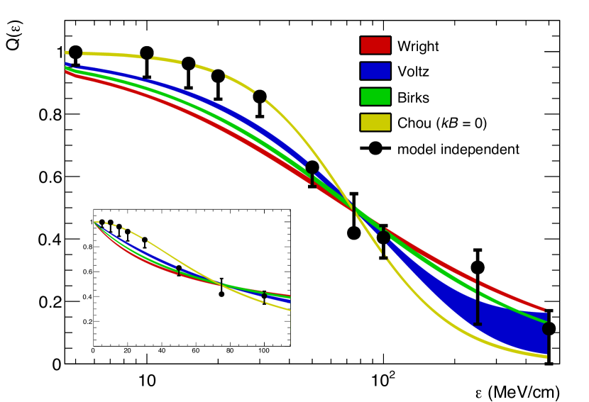
(a) SCSF-78.

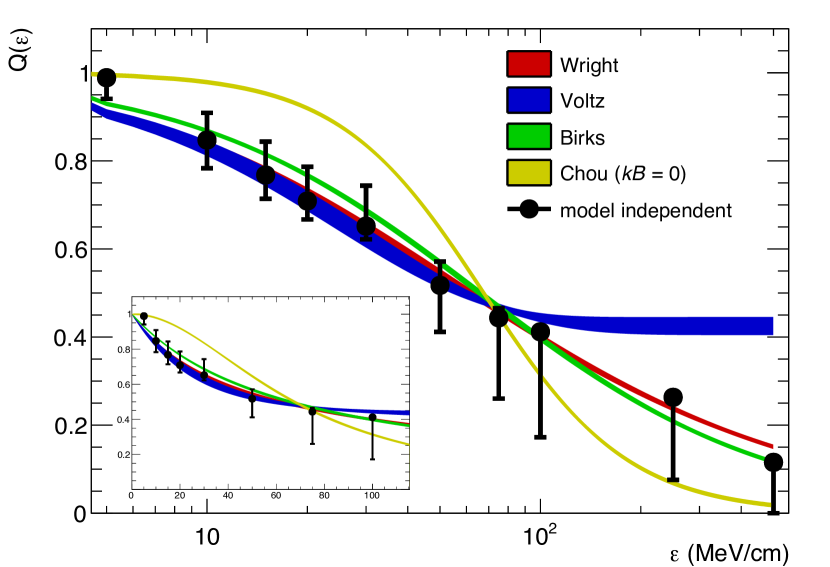
(b) BC-408.

Figure 4: $68\text{\,}\mathrm{\char 37\relax}$-credibility-interval bands for the model-dependent quenching functions listed in table 1 and the best-fit values and the smallest $68\text{\,}\mathrm{\char 37\relax}$-credibility intervals for the model-independent fits for both scintillator materials. The inset plots show the same results on a linear scale for the low-$\epsilon$ region; their axes have the same variables and units as the larger plots.

Figure 4 shows the $68\text{\,}\mathrm{\char 37\relax}$-credibility-interval bands for the model-dependent quenching functions and the best-fit values for the model-independent quenching functions for both scintillators. The bars on the model-independent results show the boundaries of the smallest $68\text{\,}\mathrm{\char 37\relax}$-credibility intervals for the value at each knot. For many of the knots, the best-fit value is near the boundary of the interval—especially those near unity. The results of the model-independent fits yield quenching functions free from any theoretically-imposed constraints. Using these results, we qualitatively evaluate each model’s ability to reproduce the data.

The model-independent quenching function for SCSF-78 has a negative second derivative at small $\epsilon$ and an inflection point at approximately $50\text{\,}\mathrm{M}\mathrm{e}\mathrm{V}\mathrm{/}\mathrm{c}\mathrm{m}$. It is inconclusive whether the quenching function approaches zero at large $\epsilon$—the value of the quenching function at $500\text{\,}\mathrm{M}\mathrm{e}\mathrm{V}\mathrm{/}\mathrm{c}\mathrm{m}$ is $1.5$ standard deviations above zero (in the posterior probability). Only Chou’s model, when $C$ is nonzero, can accommodate a negative second derivative. Figure 4(a) includes the result of a fit using Chou’s model with $kB$ fixed to zero, which is identical to the fit result reported in table 1. We see that Chou’s model is able to describe the small-$\epsilon$ behavior better than all other models.

The model-independent quenching function for BC-408 has a positive second derivative everywhere. It again is inconclusive whether it tends to zero or to a finite quenching value at large $\epsilon$—the value of the quenching function at $500\text{\,}\mathrm{M}\mathrm{e}\mathrm{V}\mathrm{/}\mathrm{c}\mathrm{m}$ is $1.1$ standard deviations above zero (in the posterior probability). These features are compatible with all the model-dependent fits. Figure 4(b) includes the result of a fit using Chou’s model with $kB$ fixed to zero—we do not show the result for a free $kB$ since it is identical to the fit with Birks’ model. We conclude that this model cannot describe the data well because it must have a negative second derivative at small $\epsilon$, which is contradicted by the model-independent result.

The model-independent quenching functions indicate that it is likely that quenching does not asymptotically drop to zero and light is produced even at large energy-deposition density.

5.2 Model comparisons

	SCSF-78		BC-408
model	$\log_{10}K$	$\Delta\log_{10}L$	$\log_{10}K$	$\Delta\log_{10}L$
Birks	—	—	—	—
Chou	$5.1\pm 0.2$	$14.6$	$-3.6\pm 0.1$	$0.2$
Chou ($kB=0$)	$7.9\pm 0.2$	$15.0$	$-14.7$ p m 0.1	$-21.3$
Wright	$-19.0\pm 0.2$	$-3.0$	$1.0\pm 0.1$	$0.1$
Voltz	$5.9\pm 0.2$	$5.6$	$1.0\pm 0.1$	$1.1$

Table 4: The log of the Bayes factor and the difference of the log of the maximum likelihood, both with respect to the fit for Birks’ model, for both scintillators.

Table 4 compares our fits for each model for both scintillators: we list both Bayes factors and the difference in maximum likelihood. We benchmark all models against Birks’ model, which is the most commonly used quenching model. If a model fits to the data better than Birks’ model, the value of $\log_{10}K$ is positive; if a model fits to the data worse than Birks’ model, it is negative. Common interpretations of Bayes factors state that $\absolutevalue{\log_{10}K}>2$ means there is decisive evidence for a conclusion; and $\absolutevalue{\log_{10}K}\approx 1$ means there is only substantial evidence [30, 31].

Our fits to the SCSF-78 data decisively prefer Chou’s and Voltz’ models to Birks’, with no strong evidence for a preference of either one over the other. However, Chou’s model with $kB$ fixed to zero is decisively preferred to all other models—its preference over Chou’s full model is a clear example of Occam’s razor. Wright’s model is strongly disfavored by our data.

These conclusions are borne out in visual comparison to the model-independent functions (figure 4(a)): Chou’s model with $kB=0$ is the only model that reproduces the model-independent function for SCSF-78 at small $\epsilon$. Our fits are most sensitive to behavior at small $\epsilon$, where a preponderance of our data is. So Chou’s model with $kB=0$ is still preferred to the other models, though it deviates the most from the model-independent behavior at medium and large $\epsilon$. To better study the behavior at large $\epsilon$, we need data using heavier and higher-charged particles, namely ions.

In fits to the BC-408 data, Birks’ model is decisively preferred to Chou’s model. This is expected: the fit with Chou’s model prefers $\sqrt{C}=0$, recreating Birks’ model but with an extra degree of freedom. This unnecessary degree of freedom is a penalty when calculating the Bayes factor—again an example of Occam’s razor. Wright’s and Voltz’ models are substantially preferred. The Bayes factor for comparing Wright’s model (with its evidence in the numerator) to Voltz’ (in the denominator) is $0.1\pm 0.1$, barely favoring Wright’s model, but inconclusively. That none of Birks’, Voltz’, or Wright’s models is decisively preferred, is also borne out in visual comparison to the model-independent function (figure 4(b)): all three models reproduce the model-independent results within their $68\text{\,}\mathrm{\char 37\relax}$ credibility intervals.

Our studies above show that quenching in SCSF-78 and in BC-408 have different dependencies on energy-deposition density. The two scintillator types differ in base material, dopant material, and dopant density—all of which can contribute to differences in quenching. No model we tested is decisively favored in fits with both scintillators. Chou’s model with $kB=0$ is most favored in fits to SCSF-78 data, but most disfavored in fits to BC-408 data. The only model to perform better than Birks’ in both fits is Voltz’.

A new model is needed to parametrize quenching in both materials. The most generic model that could fit all the features seen in the model-independent fits must allow for an asymptotic value at large $\epsilon$; the possibility of a negative second derivative at small $\epsilon$ with an inflection point where the second derivative may change sign; and different curvatures below and above this inflection point. Such a model would require at least four parameters, with all or some of them being specific to the material composition used. To fully test such a model requires new measurements at small, medium, and large $\epsilon$ for multiple scintillating materials.

6 Conclusion

We have reported measurements to precisely determine the light yield dependence on the energy-deposition density by charged particles for two different scintillating materials and presented a novel method of fitting quenching functions to this data. We have determined the parameters of four widely used quenching models—Birks’, Chou’s, Wright’s, and Voltz’—with percent-level precision. This is the first report of these parameters for the SCSF-78 scintillator; and the first report of the parameters for Chou’s, Wright’s, and Voltz’ models for the BC-408 scintillator.

We have also determined the dependence of ionization quenching on energy-deposition density for both scintillating materials using a model-independent technique. To our knowledge, this is the first model-independent determination of quenching functions. Our results indicate that quenching is highly dependent upon the scintillating material, with no common model strongly preferred for both materials; none of the most-commonly-used models describe the features of the true quenching function over the full range of energy-loss density well. Owing to their assumptions on the shape of the quenching function, these models will always overestimate quenching at either low or high energy-deposition density. The constraints of the models and that most quenching measurements are made over a small range of energy-deposition density explains why various measurements with the same scintillator type often do not agree with each other [6, 32]. Our model-independent approach allows us to determine quenching over a large range of energy-deposition densities without subregions biasing each other. New and more refined models can now be developed using our model-independent quenching functions.

7 Acknowledgments

We would like to thank O. Schulz and R. Schick for providing their HME code; P. von Doetinchem for providing the BC-408 scintillator; I. Konorov, S. Huber, and D. Levit for their help with data acquisition; K. Deiters, T. Rauber, and M. Schwarz for their support prior and during the experiment at Paul Scherrer Institute; and our late colleague D. Renker for his persistent support and many fruitful discussions.

This research was supported by the DFG Cluster of Excellence Origin and Structure of the Universe (EXC 153).

References

-
[1]
Y. N. Kharzheev, Scintillation
counters in modern high-energy physics experiments (review), Physics of
Particles and Nuclei 46 (4) (2015) 678–728.
doi:10.1134/S1063779615040048.
URL https://doi.org/10.1134/S1063779615040048 -
[2]
L. Beaulieu, S. Beddar,
Review of plastic and
liquid scintillation dosimetry for photon, electron, and proton therapy,
Physics in Medicine & Biology 61 (20) (2016) R305.
URL http://stacks.iop.org/0031-9155/61/i=20/a=R305 -
[3]