On weakly informative prior distributions for the heterogeneity parameter in Bayesian random-effects meta-analysis

Abstract

[Abstract]The normal-normal hierarchical model (NNHM) constitutes a simple and widely used framework for meta-analysis. In the common case of only few studies contributing to the meta-analysis, standard approaches to inference tend to perform poorly, and Bayesian meta-analysis has been suggested as a potential solution. The Bayesian approach, however, requires the sensible specification of prior distributions. While noninformative priors are commonly used for the overall mean effect, the use of weakly informative priors has been suggested for the heterogeneity parameter, in particular in the setting of (very) few studies. To date, however, a consensus on how to generally specify a weakly informative heterogeneity prior is lacking. Here we investigate the problem more closely and provide some guidance on prior specification.

, , , , , , , and (2021), On weakly informative prior distributions for the heterogeneity parameter in Bayesian random-effects meta-analysis, (submitted for publication), 2021.

1 Introduction

In meta-analysis, researchers commonly encounter a certain amount of variability between experiments, to a degree going beyond what could be attributed to measurement error alone. Hierarchical models are commonly used in order to account for such (“between-study”) heterogeneity.¹, ² In the present paper, we focus on the special simple case of meta-analysis within the framework of the normal-normal hierarchical model (NNHM). The NNHM approximates estimates from separate sources and their standard errors via normal distributions, and implements heterogeneity at a second level using another normal variance component. In meta-analysis applications, the NNHM provides a good approximation for many types of endpoints or effect measures.³, ⁴ The normal approximation has its limitations,⁵ some of which are less of a problem in a Bayesian context.⁶ A small number of studies tends to pose a problem especially for frequentist methods, in particular regarding the construction of confidence intervals (CIs) with good coverage properties.⁷, ⁸, ⁹, ¹⁰ A common convention is to exercise extra caution when the number of studies is small.⁹

Bayesian approaches to meta-analysis have been advocated for quite a while,¹¹, ¹², ¹³, ¹⁴, ¹⁵, ¹⁶, ¹⁷ and analyses may technically be performed using MCMC methods¹ or semi-analytical integration.¹⁸ Within the R software, for example the bayesmeta¹⁹, ²⁰ or bmeta²¹ packages are available. Performing a Bayesian analysis is not technically challenging; computations are straightforward and valid for any number of studies, although less data will mean that results are more sensitive to prior specifications (especially when it comes to variance parameters). A crucial condition is that the explicitly implemented normal approximation needs to hold, which may break down e.g. for meta-analyses of small studies.⁵, ⁶ While for large numbers of studies, the choice of prior distributions usually has little impact, for few studies the exact form of the prior distributions chosen may become crucial, as one cannot rely on the prior information being overruled by the data in that case. At least part of this problem may be considered “shared” for frequentist and Bayesian methods as long as one tries to get by without using a proper, informative prior.²² Some supposedly noninformative prior distributions can probably be argued to be less influential than others, but ultimately these are unlikely to be the best choice in few-study problems. Beyond meta-analysis, the use of informative priors for regularisation in the estimation of certain parameters is also common.²³ Especially for few studies, this may be a promising approach.²⁴ The case of “few” studies is hard to define; there is no obvious threshold, and in fact there may actually be no need to distinguish: use of an informative prior will not be harmful for analyses of “many” studies. Indeed, a proper prior is necessary irrespective of the number of studies in case the analysis requires the calculation of marginal likelihoods. In the present manuscript, we will investigate examples ranging in size between 2 and 5 studies. These are the cases where the use of an informative prior will make the greatest difference, and such situations have been discussed in the context of up to 4,⁹, 3–10,⁷ or only 2 studies.⁸

Heterogeneity priors have been investigated previously from different angles; some discussed general considerations for variance parameters¹⁵, ²⁵, ²⁶ while others motivated particular settings for specific example cases²⁷, ²⁸ or investigated commonly used settings in a systematic literature review.²⁹ The aim of the present investigation is to provide general guidance for judging and deriving weakly informative heterogeneity priors, and to suggest consensus examples for some common types of effect measures. This may also aid in the design and justification of prior settings, or the prospective pre-specification of Bayesian meta-analyses³⁰ and it may help avoid (suspicion of) post-hoc tweaking of prior assumptions.

The remainder of this article is structured as follows. In the next section, the normal-normal hierarchical model (NNHM) along with its parameters and prior distributions are formally introduced. Section 3 discusses prior distributions for the heterogeneity parameter and some general motivating considerations and implications. Section 4 motivates heterogeneity priors for a selection of common types of endpoints and effect measures based on the previously discussed ideas. In Section 5, examples of meta-analyses with different endpoints are introduced, and analyses are performed using the suggested prior settings. Section 6 closes with conclusions and recommendations.

2 The statistical model

2.1 The normal-normal hierarchical model (NNHM)

The normal-normal hierarchical model (NNHM) represents measurements $y_{i}$ from $k$ different sources using two hierarchy levels. Along with the estimates, their associated standard errors $\sigma_{i}$ need to be available. The $\sigma_{i}$ are assumed to be fixed and known (which commonly is only an approximation.⁵, ³¹) Each estimate $y_{i}$ is assumed to measure an underlying true value $\theta_{i}$, which is not necessarily identical across all $k$ measurements; (“between-study”) variability among the $\theta_{i}$ is accounted for by an additional variance component whose magnitude is given by the heterogeneity $\tau\geq 0$:

$$y_{i}|\theta_{i} \sim \mathrm{N}(\theta_{i},\sigma_{i}^{2})\mbox{,}$$ (1)

$$\theta_{i}|\mu,\tau \sim \mathrm{N}(\mu,\tau^{2})\quad\mbox{for $i=1,\ldots,k$}\mbox{,}$$ (2)

where the estimates $y_{i}$ (as well as the $\theta_{i}$) are modelled as exchangeable. The overall mean effect $\mu$ is often the figure of primary interest. By marginalizing over the $\theta_{i}$ values, the model may be written in simplified form:

$$y_{i}|\mu,\tau \sim \mathrm{N}(\mu,\,\sigma_{i}^{2}+\tau^{2})\mbox{.}$$ (3)

This is a random-effects model, which in the special case of $\tau=0$ simplifies to the common-effect model (also known as the fixed-effect model).³, ⁴, ²⁰, ³² The NNHM provides a good approximation for many types of effect measures where the estimates as well as between-study variability may be assumed to be (approximately) normally distributed.⁵

While often the aim of a meta-analysis is estimation of the overall mean $\mu$, it is sometimes useful to also infer the study-specific means $\theta_{i}$ or a prediction $\theta_{k+1}$. The amount of information gained on $\theta_{i}$ or $\theta_{k+1}$ through the joint meta-analysis depends very much on the amount of heterogeneity $\tau$. If there was no heterogeneity ($\tau=0$), then we would have $\theta_{1}=\theta_{2}=\ldots=\theta_{k+1}=\mu$, and all data would essentially contribute to the estimation of a single common parameter. If, on the other hand, $\tau$ was very large, then different parameters $\theta_{i}$ would only be very loosely connected (2), and consideration of additional data would only add very little to the estimation of any particular $\theta_{i}$ or to a prediction $\theta_{k+1}$. In between, for moderate $\tau$ values, estimates of $\theta_{i}$ are somewhat “shrunk” towards the overall mean $\mu$, and the prediction $\theta_{k+1}$ is also more tightly constrained. Estimation of the heterogeneity $\tau$ hence also has distinct effects on the so-called “shrinkage estimates” $\theta_{i}$ as well as predictions $\theta_{k+1}$.²⁰, ³³

2.2 Prior distributions

2.2.1 Effect and heterogeneity priors

In the NNHM, there are two unkowns requiring prior specification, namely the overall mean effect $\mu$ and the heterogeneity $\tau$. In the following, we will assume that the prior may be factored into $p(\mu,\tau)=p(\mu)\times p(\tau)$, implying prior independence of $\mu$ and $\tau$; note though that one may also argue in favour of a dependent prior.²², ³⁴ In a sense, dependence is often implicitly implemented e.g. in the case of log-transformed effect scales: on the back-transformed (exponentiated) scale, the amount of heterogeneity then scales with the value of the effect.

The effect prior $p(\mu)$ may often, also for technical convenience, be taken to be (improper) uniform or normal.²⁰ In case a proper, informative effect prior is used, this may also have implications for the heterogeneity prior; in particular the prior variance of $\mu$ may be relevant when considering reasonable $\tau$ values (see also Section 3.4.2 below).

Here we are first of all concerned with the prior distribution for the heterogeneity, $p(\tau)$. A number of priors have been proposed that may be considered “noninformative” in particular senses (e.g., improper uniform or Jeffreys priors, which may be motivated using invariance or information-theoretic arguments),²⁰ Sec. 2.2 but these usually cause problems especially when the number of studies ($k$) is sufficiently small, or when the computation of marginal likelihoods (or Bayes factors) is desired. In the following, we will hence be concerned with proper, (weakly) informative priors.

2.2.2 Different views of prior specification

There may be different perspectives on the role or purpose of prior specification within a Bayesian analysis; we sketch three aspects here:

(i) Epistemic point-of-view:

The posterior distribution depends on the prior via Bayes’ theorem; the prior inevitably needs to enter inference, reflecting the state of information beyond the data at hand.¹, ³⁵ Prior assumptions simply add to the line of other assumptions being made, like a normal likelihood, independence, known standard errors, etc.

(ii) Regularisation point-of-view:

The aim is to introduce “weakly informative priors, which attempt to let the data speak while being strong enough to exclude various ‘unphysical’ possibilities which, if not blocked, can take over a posterior distribution in settings with sparse data” (Gelman; 2009).³⁶ This perspective is closely connected to regularisation or penalization approaches in general.³⁷ While in the likelihood framework it may sometimes be perceived as a rather ad hoc fix, it constitutes a transparent, readily interpretable model component in the Bayesian case.

(iii) Pragmatic point-of-view:

The resulting estimates may be judged solely based on their operating characteristics (which may be frequentist or Bayesian,¹ Sec. 4.4) without worrying about their exact theoretic underpinning.

The first viewpoint is probably the most “constructive” one here, in the sense of providing guidance on sensible prior choices. An example of a regularisation approach in the NNHM context is given by the procedure proposed by Chung et al. (2013),³⁸ where regularisation is used to implement preference for positive $\tau$ values. Alternatively, one may also give preference to small $\tau$ values, as these imply a less complex model, which is the idea behind penalized complexity priors³⁹ (and which here would lead to an exponential prior). Comparisons of operating characteristics (also including frequentist approaches) were done e.g. by Friede et al. (2017).⁷ There are probably more perspectives beyond or between these three (e.g., ⁴⁰, ⁴¹). For example, meta-analyses may be thought of as constituting draws from a “population” whose associated heterogeneities are reflected in the prior distribution — an “aleatory” interpretation of (prior) probability, which may lend a somewhat frequentist flavour to the analysis. An important point to stress is that there is not necessarily a single “correct” prior: the use of different priors may be seen as basing inferences on different preconditions, and the choice of prior depends on which information one is willing to incorporate into the analysis; different analysts may hence draw different conclusions from the same data, when these are founded on differing prior beliefs.⁴² In a sense, the posterior inherits its meaning from the prior to some extent.⁴³ Other common shortcuts taken or approximations and asymptotics relied upon may in fact often be potentially more influential and relevant than the choice among the (usually limited) set of reasonable prior distributions (see, e.g., Jackson and White (2018)⁵).

2.2.3 Implications for interval estimation

While (frequentist) confidence intervals aim to provide coverage of the true parameter uniformly, independent of the actual current parameter value, this is generally not the case for (Bayesian) credible intervals. In some cases, it is possible to specify (often improper) priors leading to posterior distributions that also provide proper frequentist coverage, but usually such a prior is not available.⁴⁴ Credible intervals are calibrated and yield proper coverage on average across the prior distribution; for the point-wise coverage this means that there may be overcoverage in certain regions of parameter space and undercoverage in others.²⁰, ⁴⁵, ⁴⁶, ⁴⁷ For example, in the present case this may mean that long-run coverage may be above the nominal level if data were repeatedly generated based on heterogeneity values from the lower end of the prior range, and below the nominal level otherwise.

3 Heterogeneity priors

3.1 Aim

For meta-analyses involving many studies (large $k$), the choice of prior distribution often has little impact, and an (improper) uniform prior for $\tau$ may be a good choice, not least due to its invariance property.²⁰, ²⁵ Here we are concerned first of all with the case of few studies (small $k$); a uniform prior may not actually be an option here, as it requires $k\geq 3$ studies in order to yield a proper, integrable posterior,²⁵ and it may otherwise generally be considered overly conservative.⁷, ⁸, ²⁵ Similar problems arise also with the Jeffreys prior for the NNHM model;²⁰ Sec. 2.2 this kind of issue is common in Bayesian analysis.²³ Another case where a proper, weakly informative prior may be required (not only for few studies) is when marginal likelihoods or Bayes factors are of interest.

While the availability of a “noninformative” prior comes with a certain convenience (one less issue to worry about), in the present case its failure to provide reasonable estimates in certain instances will often appear somewhat contradictory to common sense. The introduction of an informative prior then may entail a trade-off of the introduced regularisation versus simplicity and robustness. On the other hand, the explicit consideration of relevant prior information may also be seen as an advantage.

From a merely “technical” perspective, a heterogeneity prior must (in order to ensure integrability of the posterior) have a shorter-than-uniform upper tail (an eventually decreasing, integrable density function) and also an integrable density towards zero. In that spirit, it may also make sense to consider near-origin- and upper-tail-behaviours separately. While an (improper) uniform prior may be considered noninformative for several reasons (e.g., due to its scale-invariance property²⁰ Sec. 2.2), its overly heavy upper tail may also be considered “anti-conservative”.⁴⁸ On the other hand, it may be possible to “rescue” some of the desirable behaviour and robustness e.g. by the use of heavy-tailed priors.⁴⁹ Besides upper-tail considerations, priors may also behave quite differently near zero; for example, depending on whether the prior density approaches zero, a finite value, or infinity. A finite prior density may ensure a near-zero behaviour roughly like a uniform prior, while a zero density may be useful e.g. in bounding maximum-a-posteriori (MAP) point estimates away from zero;³⁸ in particular from the regularisation perspective, the prior density’s derivative near zero may also be of interest (as it determines how small $\tau$ values may be pushed towards or away from zero).

While the concept of “weak informativeness” remains somewhat elusive (just like that of a “noninformative” prior), the information content (or “vagueness”) of a prior is commonly related to its variance, its entropy,⁵⁰ or its associated effective sample size (ESS).⁵¹, ⁵² In many cases it is also helpful to consider the informativeness of a prior relative to a reference,⁵³ for example, a unit information prior.²⁶, ⁵⁴ Since the posterior draws its interpretation in part from the prior, it is important to make the prior specification plausible and transparent. Following the parsimony principle (Ockham’s razor), it may be contructive to seek the (in some sense) simplest prior distribution within any relevant constraints.⁵⁵ Possible approaches to implement such a notion in practice may work, e.g., via maximization of the entropy,⁵⁰ pre-specification of an effective sample size,⁵¹, ⁵² or matching of moments.

Despite the aim of a weakly informative formulation, one should also anticipate the case where the data have little information to add, so that the posterior closely resembles the prior and hence the analysis results are largely determined by the prior settings. This may happen especially in cases of few studies and is also suggested in some of the examples that will be discussed below (see Figure 8); such cases highlight the importance of a transparent and convincing prior specification.

In the remainder of this section, we aim to facilitate a structured approach to interpreting heterogeneity and specifying heterogeneity prior distributions by pointing out relevant perspectives and highlighting consequences of certain heterogeneity settings. Similar ideas are to some degree also utilized in prior elicitation in general.⁵⁶, ⁵⁷ A set of guiding questions is eventually suggested in Table 6.

3.2 General properties of the NNHM

When considering prior distributions for the heterogeneity $\tau$, it is useful to recall that $\tau\geq 0$ is a scale parameter, and that its square $\tau^{2}$ denotes a variance component within the NNHM. Immediate associations of variance priors useful in a simple normal model however may be misleading: inverse-gamma (or inverse-$\chi^{2}$) distributions are usually not recommended, as these arise as conjugate distributions only in related, yet distinctly different circumstances. An inverse-gamma distribution is conjugate in the simple case of estimating the variance of a normal distribution with known mean.¹ In such a case, an unequal pair of two data points for example implies that the variance must be positive (a zero variance would have a zero likelihood); in the present NNHM context, however, unequal $y_{i}$ values may be consistent with zero heterogeneity ($\tau=0$), so that such priors are not a natural choice here, and their use is generally discouraged.², ²⁵, ⁵⁸, ⁵⁹ Supposedly noninformative settings based on inverse-gamma distributions commonly tend to result in sensitivity to specification details,²⁵ and often too much probability is allocated to very large heterogeneity values.⁶⁰

For uniform or normal effect prior distributions, the resulting conditional effect posterior $p(\mu|\tau,y)$ again is normal. While for increasing $\tau$ the (conditional) posterior mean of $\mu$ shifts from the inverse-variance weighted mean towards the unweighted average of the estimates $y_{i}$, the (conditional) posterior variance of $\mu$ is proportional to $\tau$.²⁰ At the same time, larger heterogeneity values also imply wider prediction intervals and less shrinkage ¹⁶, ²⁰, ⁶¹, ⁶², ⁶³ (see also Section 2.1). Varying $\tau$ between zero and infinity essentially also means varying between the extremes of pooled and separate analyses of individual studies. In a sense, overestimation of $\tau$ may hence often be considered a “conservative” or “less harmful” form of bias. In that spirit, one might argue that —within reasonable limits— a prior that is stochastically larger than another is also more conservative.⁶⁴ A simple way to implement stochastically ordered distribution families is by using parametisations that include a scale parameter.⁶⁵ Sec. VII.6.2 Use of a scale parameter does not actually impose a restriction; if not already included in the parametrisation, it may easily be introduced. Note that simple re-scaling of a prior distribution $p(\tau)$ then also implies a (re)scaling of the corresponding marginal prior predictive distributions $p(\theta_{i}|\mu)$ by the same factor. In general, stochastically ordered priors also imply the same ordering for the resulting posteriors.⁶³, ⁶⁶, ⁶⁷ Consideration of stochastically ordered alternative priors may hence also offer a framework for sensitivity analyses (see also Appendix D.4).

3.3 Reasonable (proper) distributional families

A simple way to implement the “technical” requirements (as suggested in Section 3.1) may be to require roughly uniform behaviour near zero (implying indifference among small heterogeneity values on the $\tau$ scale and ensuring integrability in the lower tail), and a monotonically decaying tail with increasing heterogeneity values (implying decreasing probability for increasing $\tau$ values and ensuring integrability in the upper tail). This may be achieved e.g. by using half-normal, half-Student-$t$, half-Cauchy, half-logistic, exponential or Lomax distributions. A sample of such distributions is sketched in Figure 1.

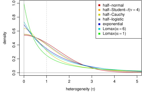
Figure 1: A selection of potential probability densities for the heterogeneity. All distributions are scaled so that their prior median is at unity ($\tau\!=\!1$, dashed line; see also Table 4).

Note that for comparability, the distributions in the figure are all scaled such that they have a common median of $1$; their corresponding parameters are also listed in Table 4 below. In particular, half-normal, half-Student-$t$, or half-Cauchy distributions have been recommended as appropriate families within the NNHM, also due to favourable frequentist properties.², ²⁵, ⁵⁸ The half-Student-$t$ distribution (including the half-Cauchy as a special case, and the half-normal as a limiting case) may be derived as conditionally conjugate distributions in an extended parametrisation of the NNHM.² Sec. 19.6 The exponential distribution might be motivated as the maximum entropy distribution for a pre-specified prior expectation,⁵⁰ or as the penalised complexity prior.³⁹ The half-logistic distribution combines a zero derivative (implying near-uniform behaviour) at the origin with an upper tail behaviour close to that of an exponential distribution.

Half-Student-$t$ and Lomax distributions here may be considered as heavy-tailed variants of the half-normal and exponential distributions, respectively. In the spirit of a contaminated prior, encompassing priors “close to an elicited one”,⁶⁸⁶⁹ Sec. 3.5.3 these may also be motivated as scale mixtures, where the (exponential or half-normal) scale parameter is associated with some variability or uncertainty. The scale mixture connection is also derived in detail in Appendix C below. The special case of a Lomax($\alpha\!=\!1$) distribution also coincides with the form of prior distribution suggested by DuMouchel (a log-logistic prior for $\tau$).⁷⁰, ⁷¹ Similarly, the exponential distribution may also be motivated as a scale mixture of a half-normal distribution with Rayleigh-distributed scale. The use of heavy-tailed prior distributions has the advantage of ensuring some degree of robustness against prior misspecification (or prior/data conflict)⁴⁹ at the cost of sacrificing some of its “regularisation” power. Another simple way of implementing some degree of robustness is by combining “informative” and “heavy-tailed” elements in a two-component mixture distribution.⁷², ⁷³

Another simple and common prior distribution is the (proper) bounded uniform distribution defined on an interval $[0,a]$. It inherits certain qualities from the (improper) uniform distribution, but it introduces a sharp cutoff at the upper bound $a$, which may be hard to motivate or justify. Although, if the bound is large enough, then it may be very reasonable (e.g. for log-ORs).

Among the above examples, the Student-$t$ and Lomax distributions possess “shape” parameters in addition to scale parameters, which here essentially regulate the degree of heavy-tailedness. If considered desirable, more complex prior assumptions may be implemented using more complex distributions, e.g., using folded non-central Student-$t$ distributions with a non-zero mode,², ²⁵, ⁵⁸ however, additional degrees of complexity would probably require solid justification to be convincing. In the context of a penalisation interpretation of the prior, a mode at zero also implies a corresponding “penalty term” that is monotonically increasing in $\tau$; this applies e.g. for a penalized-complexity prior³⁹ that aims to give preference to sparse models. In empirical investigations based on meta-analyses archived in the Cochrane Database of Systematic Reviews, log-Normal and log-Student-$t_{5}$ distributions have been fitted to empirical data.⁷⁴, ⁷⁵ The log-normal and log-$t$ distributions here were found to fit the predictive distributions best, however, only few alternatives (log-normal, log-$t_{5}$ and inverse-gamma,⁷⁴ or log-normal, inverse-gamma and gamma distributions⁷⁵ for $\tau^{2}$) were considered as candidates in these comparisons. Some properties of the distributions discussed here are also listed in Appendix B.

In practice, the half-normal distribution is quite commonly used; the reasons for its popularity are probably its simple and familiar form, its near-uniform behaviour at the origin along with a reasonably quickly decaying upper tail, as well as considerations of numerical stability. In the following, we will focus mostly on half-normal distributions. In our experience, minor differences between similar prior densities are of rather minor practical relevance, while it is most important what heterogeneity ranges the bulk of prior probability is assigned to.

When eventually formulating prior assumptions in terms of a parametric prior probability distribution, it is first of all necessary to be able to judge the meaning and implications of certain heterogeneity settings; these issues will be discussed in the following section.

3.4 Interpreting heterogeneity values

3.4.1 Units of $\tau$

Informative priors naturally always need to be considered in the context of the endpoint under consideration. In order to specify a sensible prior for $\tau$, it is important to recapitulate its role in the NNHM (see Section 2.1). The heterogeneity $\tau$ is a scale parameter that relates to the probable size of differences (between-study differences) in effects ($\theta_{i}$ and $\mu$; see equation (2)). With that, the units of measurements ($y_{i}$), effects ($\theta_{i}$, $\mu$) and heterogeneity ($\tau$) are the same; if the effect is measured, say, in metres, then so is the heterogeneity. Or both may be dimensionless, as e.g. in the case of log-transformed ratios (like log-odds-ratios (log-ORs), log-incidence-rate-ratios (log-IRRs), log-hazard-ratios (log-HRs),…) or standardized mean differences (SMDs). One may in fact argue that the nature of the effect scale is the most important aspect to consider for prior specification.²⁴ In case the effects $y_{i}$ have been transformed prior to analysis, then it is often useful to consider implications on the back-transformed scale. Transformations are usually introduced to achieve a better fit to the normality assumptions within the NNHM; for example, using logarithmic or arcsine transforms.³, ⁴, ⁷⁶ In such cases, also considering the back-transformed (exponential or sine) effect scales is often instructive.

In case the effect scale has definite upper and lower bounds (which is often the case e.g. for endpoints measured as scores), this also provides information on the plausible (and possible) between-study variability. In case of bounded scales, it may for example be useful to consider the extreme cases of a continuous uniform distribution across the considered range (which would have standard deviation $\frac{b-a}{\sqrt{12}}=\frac{b-a}{3.46}$, where $a$ and $b$ are the lower and upper bounds, respectively), or a discrete distribution with probabilities of $\frac{1}{2}$ concentrated at both margins $a$ and $b$ (which would have standard deviation $\frac{b-a}{2}$). Such considerations may define absolute “worst-case” settings for the heterogeneity. Any normal approximation employed on a bounded parameter space with a standard deviation of, say, $>\frac{b-a}{4}$ would inevitably have substantial overlap with out-of-domain values; any heterogeneity value that is not $\ll\frac{b-a}{4}$ should raise suspicion and might actually call for a different approach (e.g., transformation to a different parameter space).

3.4.2 Magnitudes of other effects

Relevant hints may originate from considering the magnitude of other (known or plausible) effects of interventions or covariates. The reasonable range for the overall mean effect $\mu$ may also have implications for the expected range of study-specific means $\theta_{i}$; in case an informative prior for $\mu$ is used (or is at least plausible), its variance may help constraining also the between-trial variability. Heterogeneity may often be attributed to differences in the composition of the populations underlying each estimate, and the distribution of relevant covariates within (which may be observed or unobserved). If the observed heterogeneity is assumed to be due to different constitutions of populations, then the heterogeneity relates to accumulated effects of associated covariates. With that, within- and between-study variability in effects are related to within- and between-study differences among subjects and the plausible magnitude of covariates’ effects. For example, if a treatment effect is known to differ between males and females by a certain amount, this difference between genders may help judging or motivating plausible magnitudes of effect differences between studies. In case the variability between centers within the same study has been investigated, this may also provide a hint on between-study variability (which will then most likely be larger).

3.4.3 Implications of a fixed heterogeneity value

Specific values of the heterogeneity $\tau$ may be judged and compared based on the implied distribution of true effects $\theta_{i}$, which is given by the (conditional) prior predictive distribution $p(\theta_{i}|\mu,\tau)$ (see equation (2)), where $\tau$ defines the distribution’s standard deviation. The effects $\theta_{i}$ (conditional on $\mu$) then vary within a range of $\mu\pm 1.96\tau$ with 95% probability. For a randomly picked pair of effects ($\theta_{i}$ and $\theta_{j}$), their difference ($\theta_{i}-\theta_{j}$) follows a $\mathrm{N}(0,2\tau^{2})$-distribution (2), and their absolute difference $|\theta_{i}-\theta_{j}|$ then has a median of $0.95\tau$. Quite commonly, the effects $\theta_{i}$ are transformed prior to analysis, so that it may be helpful to consider the implications on the back-transformed scale. A very common example is the logarithmic transformation, which is often used for analyses involving e.g. odds ratios (ORs), relative risks (RRs) or hazard ratios (HRs), and where the inverse transform is the exponential function. 95% predictive intervals and median differences are shown for a range of $\tau$ values in Table 1 along with the corresponding exponentiated figures.

Table 1: Implications of certain fixed heterogeneity values $\tau$ on the probable ranges of true effects $\theta_{i}$ (conditional prior predictive distributions) and the corresponding exponentiated ranges (the latter are relevant for log-transformed effect scales).

	95% predictive interval		random pair $|\theta_{i}-\theta_{j}|$
$\tau$	$\theta_{i}-\mu$	$\exp(\theta_{i}-\mu)$	median	$\exp(\mbox{median})$
0.1	[-0.20, 0.20]	[0.82, 1.22]	0.10	1.10
0.2	[-0.39, 0.39]	[0.68, 1.48]	0.19	1.21
0.5	[-0.98, 0.98]	[0.38, 2.66]	0.48	1.61
1.0	[-1.96, 1.96]	[0.14, 7.10]	0.95	2.60
2.0	[-3.92, 3.92]	[0.020, 50.4]	1.91	6.74

An extensive discussion of these conditional distributions is given in Spiegelhalter et al. (2004).¹⁵ Sec. 5.7 By working out what range of $\theta_{i}$ values is expected, or what difference between a randomly picked pair of $\theta_{i}$ values is expected, corresponding plausible ranges of $\tau$ values may be determined. Based on such considerations, Spiegelhalter et al. (2004)¹⁵ categorized ranges of $\tau$ values in the context of log-ORs as “reasonable”, “fairly high” or “fairly extreme” as shown in Table 2.

Table 2: Categories of heterogeneity and corresponding $\tau$ ranges in the context of log-ORs, according to Spiegelhalter et al. (2004).¹⁵ Sec. 5.7

category	range
“reasonable”	$0.1<\tau<0.5$
“fairly high”	$0.5<\tau<1.0$
“fairly extreme”	$\tau>1.0$

Such investigations may help judging what $\tau$ values are reasonable or unrealistic and with that may help specifying e.g. the heterogeneity prior’s tail quantiles.

For example, Prevost et al. (2000)²⁷ Sec. 4 aimed to constrain the predictive interval ($\exp(\theta_{i}-\mu)$) to a range of $[0.5,\,2.0]$, which is achieved for $\tau=0.35$. Considering this range as extreme and unlikely, a half-Normal prior with scale $0.18$ (implying $\mathrm{P}(\tau\leq 0.35)=0.95$) was eventually suggested for a log-RR. R code to illustrate these arguments using Monte Carlo sampling and exact calculations is provided in Appendix D.1.

3.4.4 Implications of a heterogeneity distribution

Besides considering the conditional distribution for fixed $\tau$ values ($p(\theta_{i}|\mu,\tau)$, see previous subsection), one may also investigate the marginal prior predictive distribution $p(\theta_{i}|\mu)$, marginalized over a particular heterogeneity prior, which technically results as the integral $p(\theta_{i}|\mu)=\int_{0}^{\infty}p(\theta_{i}|\mu,\tau)\,p(\tau)\,\mathrm{d}\tau$. Since $p(\theta_{i}|\mu,\tau)$ is normal (2), the marginal $p(\theta_{i}|\mu)$ is a normal (scale) mixture distribution. Its form may usually either be derived numerically,¹⁸, ¹⁹, ²⁰ or it may easily be explored using collapsed Gibbs sampling, that is, generating a Monte Carlo sample by repeatedly sampling from the heterogeneity prior ($p(\tau)$), and subseqently from the conditional predictive distribution ($p(\theta_{i}|\tau)$). Investigating the marginal prior predictive distribution may help judging the prior scale or distributional family.

Table 3: Implications of a range of half-normal heterogeneity priors $p(\tau)$ on probable values of heterogeneity $\tau$ and predicted effects $\theta_{i}$ (marginal prior predictive distributions). The three rightmost columns show the corresponding probabilities for the three categories from Table 2.

	heterogeneity $\tau$			95% predictive interval		category probability (%)
$p(\tau)$	median	mean	95% quant.	$\theta_{i}-\mu$	$\exp(\theta_{i}-\mu)$	reason- able	fairly high	fairly extreme
half-normal(0.1)	0.07	0.08	0.20	[-0.22, 0.22]	[0.80, 1.24]	32	00	00
half-normal(0.2)	0.13	0.16	0.39	[-0.44, 0.44]	[0.65, 1.55]	60	01	00
half-normal(0.5)	0.34	0.40	0.98	[-1.09, 1.09]	[0.34, 2.98]	52	27	05
half-normal(1.0)	0.67	0.80	1.96	[-2.18, 2.18]	[0.11, 8.89]	30	30	32
half-normal(2.0)	1.35	1.60	3.92	[-4.37, 4.37]	[0.013, 79.0]	16	19	62

Table 3 illustrates a range of prior predictive distributions for a set of half-normal priors that differ in their scale. The implied probabilities for the (log-OR) categories shown in Table 2 are also given. Note that a simple re-scaling of the heterogeneity prior implies proportional scaling of mean and quantiles for $\tau$ as well as $\theta_{i}$ (as can be seen in Table 3). In this spirit, Dias et al. (2013)²⁸ for example proposed a half-normal(0.32)-prior for a log-OR based on the implied prediction interval for $\exp(\theta_{i}-\mu)$ of $[0.5,\,2.0]$. R code to illustrate these arguments using Monte Carlo sampling and exact calculations is provided in Appendix D.2

Table 4: Implications of a range of heterogeneity priors $p(\tau)$ from different families on probable values of of heterogeneity $\tau$ and predicted effects $\theta_{i}$ (marginal prior predictive distributions). For comparability, the different priors are all scaled to a common median of $1.0$. Except for the exponential distribution, which is commonly parameterized by its rate (or inverse scale), all distributions have a scale parameter.

		heterogeneity $\tau$			95% predictive interval
$p(\tau)$	scale	median	mean	95% quant.	$\theta_{i}-\mu$	$\exp(\theta_{i}-\mu)$
half-normal(1.48)	1.48	1.00	1.18	02.91	[-3.24, 3.24]	[0.039, 25.5]
half-Student-$t_{\nu=4}$(1.35)	1.35	1.00	1.28	03.75	[-3.85, 3.85]	[0.021, 46.8]
half-Cauchy(1.00)	1.00	1.00		12.71	[-10.10, 10.10]	[0.000 041, 24 371]
half-logistic(0.91)	0.91	1.00	1.26	03.33	[-3.55, 3.55]	[0.029, 34.7]
exponential(0.69)	1.44	1.00	1.44	04.32	[-4.33, 4.33]	[0.013, 75.9]
Lomaxα=6(8.17)	8.17	1.00	1.63	05.29	[-5.04, 5.04]	[0.0065, 155]
Lomaxα=1(1.00)	1.00	1.00		19.00	[-14.74, 14.74]	[0.000 000 40, 2 520 157]

Similarly, Table 4 illustrates a range of prior predictive distributions for a set of heterogeneity priors from different distributional families; what they have in common is the prior median of $1.0$ for $\tau$. Quantiles or mean of $\tau$ or $\theta_{i}$ for other scalings of $p(\tau)$ may be derived by proportional re-scaling (as in Table 3). For example, a half-Cauchy distribution that has its median heterogeneity matched to that of a half-normal distribution requires a scale parameter that is smaller by a factor of $\approx 2/3$. From the table, one can also read off the ratio of 95% quantile over the median, which may be a useful indicator of the heavy-tailedness of the different distribution families. The distributions from Table 4 are also illustrated in Figure 1. Some additional properties of these distributions are provided in Appendix B.

Different distributional families for the prior $p(\tau)$ imply differing marginal prior predictive distributions $p(\theta_{i}|\mu,\tau)$. Concrete prior information on $p(\theta_{i}|\mu,\tau)$ then may help constraining the shape of $p(\tau)$, however, the prior family may also be selected based on considerations of heavy-tailedness, near-zero behaviour, or simplicity.

3.4.5 The role of the unit information standard deviation (UISD)

Consider the simple case of an effect measure that for each study is determined as an average of independent identically distributed observations. In such a case, the associated standard error is simply of the form

$$\sigma_{i}\;=\;\frac{\sigma_{\mathbb{1}}}{\sqrt{n_{i}}}\mbox{,}$$ (4)

where $n_{i}$ is the sample size, and $\sigma_{\mathbb{1}}$ is the common “population” standard deviation of each single observation that was averaged over. This figure describes the population-, or within-study-standard deviation,⁵⁴ which for the moment we take to be constant across studies. This figure is also called the unit information standard deviation (UISD), as it relates to an observational unit’s contribution to a study’s likelihood. One may now relate the heterogeneity $\tau$ to $\sigma_{\mathbb{1}}$ and ask whether the between-study variability ($\tau$) is likely to exceed the within-study variability ($\sigma_{\mathbb{1}}$), or what ratios of these two are plausible. Figure 2 illustrates the relationship of within-study and between-study standard deviations $\sigma_{\mathbb{1}}$ and $\tau$. Usually, one would expect $\tau\!\ll\!\sigma_{\mathbb{1}}$, implying that while study means ($\theta_{i}$) may differ to some degree, the distributions of subjects within studies will still be largely overlapping (see Figure 2, left panel). In that sense, the UISD $\sigma_{\mathbb{1}}$ may constitute an important “landmark” on the heterogeneity continuum and thus may help constraining the range of plausible heterogeneity values.²⁶

(a) $\;\tau\ll\sigma_{\mathbb{1}}$         (b) $\;\tau\gg\sigma_{\mathbb{1}}$
       

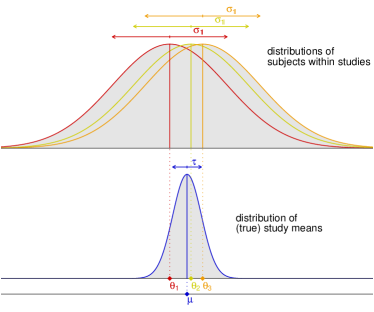
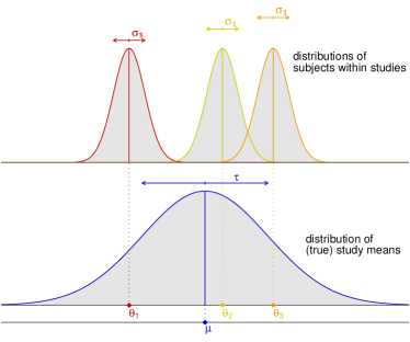
Figure 2: Illustration of the relationship of between-study heterogeneity $\tau$ and unit information standard deviation (UISD) $\sigma_{\mathbb{1}}$. The left panel (a) shows the commonly expected setup, in which the heterogeneity $\tau$ is relatively small compared to the within-study standard deviation ($\tau\!\ll\!\sigma_{\mathbb{1}}$). The right panel (b) shows that a larger $\tau$ would imply that the distributions of subjects from different studies were eventually barely overlapping. Note that the eventual estimates ($y_{i}$) resulting from the different studies then may have different standard errors $\sigma_{i}=\frac{\sigma_{\mathbb{1}}}{\sqrt{n_{i}}}<\sigma_{\mathbb{1}}$ associated, depending on the studies’ sample sizes $n_{i}$.

This concept of within-study standard deviation may be extended to other types of effect scales — for example, the standard error of a log-OR derived from a $2\times 2$-table is approximately given by $\sigma_{i}=\frac{4}{\sqrt{n_{i}}}$, so that, heuristically, the UISD here equals $\sigma_{\mathbb{1}}\!=\!4$ per subject (at least).²⁰ Appendix A.1 Sometimes it may also make more sense to define UISDs not per subject but rather per event (see also Appendix A.3 for an example), but care also needs to be taken in order not to confuse these two figures. For a given set of log-OR estimates, the UISD may alternatively also be investigated by inverting equation 4 (see also (6) and the examples in Section 5.3 below).

Another link may be drawn between $\sigma_{\mathbb{1}}$ and $\tau$ via shrinkage estimation (see Section 2.1) and the consideration of prior effective sample sizes.⁵², ⁷⁷ Consider the case where a meta-analysis of $k$ studies is available, and a new ($k\!+\!1$th) study is conducted. The previous meta-analysis of course provides (prior) information on the new study’s estimate $\theta_{k+1}$, the exact amount of which is determined by the number of studies $k$, their sample sizes $n_{i}$, the UISD $\sigma_{\mathbb{1}}$, but also by the amount of heterogeneity.³³, ⁷² If $\tau$ is large, then separate studies are only loosely related and the previous data add little information. If on the other hand $\tau$ is very small (i.e., studies are almost homogeneous), then they may contribute a lot of information. With that, the amount of heterogeneity is related to whether studies should rather be pooled or viewed as essentially independent pieces of information. One may then consider the idealized limiting case of infinitely many ($k\rightarrow\infty$) infinitely large ($n_{i}\rightarrow\infty$) studies as the previous data source, so that the amount of contributed information solely depends on $\tau$. In that case, the historical data may be thought of as effectively contributing a number of $n^{\star}_{\infty}$ additional subjects to the $k\!+\!1$th study. This prior maximum sample size then relates to $\sigma_{\mathbb{1}}$ and $\tau$ as⁷⁷

$$\frac{\tau}{\sigma_{\mathbb{1}}}\;=\;\frac{1}{\sqrt{n^{\star}_{\infty}}}\mbox{.}$$ (5)

Table 5 illustrates this relationship.

Table 5: Correspondence between prior maximum sample sizes ($n^{\star}_{\infty}$) and the magnitude of the heterogeneity ($\tau$) relative to the unit information standard deviation (UISD) ($\sigma_{\mathbb{1}}$) (see (5)).⁷⁷

$\tau/\sigma_{\mathbb{1}}\quad$	0	1/16	1/8	1/4	1/2	1	$\infty$
$n^{\star}_{\infty}$	$\infty$	256	64	16	4	1	0

For example, if in the ideal case (i.e., $k=\infty$, $n_{i}=\infty$) the additional data should add information equivalent to at most 16 subjects, then this would correspond to $\tau$ amounting to at most a quarter of $\sigma_{\mathbb{1}}$. If one has an idea of how much information a meta-analysis may (or should) contribute to a single study’s shrinkage estimate (in the idealized case of very many very large studies), then such considerations may help constraining probable magnitudes of $\tau$, or associating probabilities with ranges of $\tau$ values.

Note that a number of priors have been proposed which are defined relative to the magnitude of the $\sigma_{i}$ values (or their harmonic mean), e.g., the Jeffreys, DuMouchel or uniform shrinkage priors.²⁰ Sec. 2.2 In view of the above arguments, it might also make sense to define priors relative to the UISD, or its estimated value. Inverting (4) yields $\sigma_{\mathbb{1}}=\sqrt{n_{i}\,\sigma_{i}^{2}\,}$ for a single study, and based on a given data set we suggest the more general empirical estimate

$$s_{\mathbb{1}}\;=\;\sqrt{\bar{n}\;\bar{s}_{\mathrm{h}}^{2}\,}\;=\;\sqrt{\frac{\sum_{i=1}^{k}n_{i}}{\sum_{i=1}^{k}\sigma_{i}^{-2}}}$$ (6)

where $\bar{n}=\frac{1}{k}\sum_{i=1}^{k}n_{i}$ is the average (arithmetic mean) sample size, and $\bar{s}_{\mathrm{h}}^{2}=\bigl{(}\frac{1}{k}\sum_{i=1}^{k}\sigma_{i}^{-2}\bigr{)}^{-1}$ is the harmonic mean of the squared standard errors (variances). This estimator is defined so that in the special case of a common-effect analysis (i.e., assuming $\tau=0$), the overall mean estimate’s variance (which then is given by $\bigl{(}\sum_{i=1}^{k}\sigma_{i}^{-2}\bigr{)}^{-1}$) consistently also equals $\frac{s_{\mathbb{1}}^{2}}{\sum_{i}n_{i}}$.

3.4.6 Empirical information on $\tau$

Empirical data, e.g. from earlier investigations in a related area,⁷⁸ may also contribute to a-priori information. Informative priors based on empirical information have been derived for standardized mean differences (SMDs) and log-ORs in medical applications by investigating large numbers of meta-analyses published in the Cochrane Database of Systematic Reviews by Rhodes et al. (2015)⁷⁴ and Turner et al. (2015).⁷⁵ Additional evidence for certain types of effect scales may be found e.g. in the works by Pullenayegum (2011),³⁴ Turner et al. (2012),⁷⁹ Kontopantelis et al. (2013),⁸⁰ Steel et al. (2015),⁸¹ van Erp et al. (2017),⁸² Seide et al. (2019),⁸³, ⁸⁴ and Günhan et al. (2020).⁸⁵ Note that some references provide information directly on the heterogeneity parameter, while others summarize estimates of heterogeneity.

Empirical information often entails the question of how representative the external information is for the study at hand, or what may be the relevant data subset, or what to do if no such sample may be available. In terms of the epistemic view discussed in Section 2.2.2, the inclusion of empirical evidence in the prior specification affects the interpretation of the prior, and with that, of the posterior. Empirical data may then often be seen as a somewhat complementary source of evidence. When there is doubt about the immediate applicability of empirical information for the problem at hand, this may also be reflected e.g. in a robustified two-component mixture prior.⁷², ⁷³

3.5 Guiding questions

In order to summarize the above arguments, Table 6 lists some guiding questions that may aid in structuring the specification of a prior for the heterogeneity. These are mostly based on the arguments laid out in Sections 3.3 and 3.4. Firstly, plausible heterogeneity magnitudes (in terms of $\tau$ or $\theta_{i}$ ranges) need to be be determined. These reflections may then also help choosing a parametric family for the prior, or the distributional family may also be selected based on considerations of near-zero behaviour, heavy-tailedness or simplicity. Beyond the mere type of endpoint or effect measure, the context also may determine whether smaller or larger amounts of heterogeneity are to be expected, e.g., depending on whether studies’ designs and populations were similar. Special considerations in the context of specific common types of effect scales are discussed in detail in Section 4. These are then illustrated using actual data examples in Section 5.

Table 6: Some guiding questions for judging reasonable prior distributions for the heterogeneity parameter $\tau$.

Prior information:
(i)	What is the effect scale, what (between-study) differences are expected or plausible?
(ii)	What is the magnitude of other known (or plausible) effects? Do these provide guidance? Is an informative effect prior used? If so, what is its variance? Does it provide guidance?
(iii)	Is a plausible “unit information standard deviation (UISD)” available? Does it provide guidance?
(iv)	Is relevant external empirical information on heterogeneity available? Should it be considered in the analysis?
Translation into a prior probability distribution:
(v)	Does the prior information help pinpointing prior quantiles (of $\tau$)?
(vi)	Does the prior information help pinpointing prior predictive quantiles (of $\theta_{i}$)?
(vii)	Does the prior information suggest particular properties for the prior (-density)? (Monotonicity? A non-zero mode? A heavy tail? Certain near-zero behaviour? …)

4 Motivating heterogeneity priors in various settings

4.1 Means and mean differences

This general case covers endpoints measured on absolute scales, hence it is not possible to give universally applicable advice on a plausible prior scale. For example, the same analysis may require different scalings of the prior depending on whether an endpoint is expressed, say, in terms of hours or minutes. In particular, in case of effects that are defined as averages, the UISD (see also Section 3.4.5) may provide some guidance; if standard errors $\sigma_{i}$ scale with sample size ($\sigma_{i}\approx\frac{\sigma_{\mathbb{1}}}{\sqrt{n_{i}}}$, see also equation (4)), then $\sigma_{\mathbb{1}}$ (or an estimate $s_{\mathbb{1}}$, (6)) may provide some orientation based on the considered (or other related) data. Relating effects to “within-population standard deviations” is actually an approach that is also formalized in the case of standardized mean differences (SMDs); see the following section.

Mean differences are another very common special case. These are often used in order to “normalize” outcomes; for example, in controlled clinical trials, each study’s treatment group is usually related to a control group in order to express the treatment effect relative to the unexposed group. In the simplest case, the study’s outcome then is defined as $y_{i}=\bar{x}_{2;i}-\bar{x}_{1;i}$, where $\bar{x}_{1;i}$ and $\bar{x}_{2;i}$ are the $i$th study’s averages from control and treatment group, respectively. When considering UISDs, the relevant sample size will then result as the sum of the two treatment groups’ sizes ($n_{i}=n_{1;i}+n_{2;i}$). In the simple case of two equally-sized groups ($n_{1;i}=n_{2;i}=\frac{n_{i}}{2}$) and equal variances within groups (so that $\mathrm{Var}(\bar{x}_{1;i})=\mathrm{Var}(\bar{x}_{2;i})=\frac{\sigma_{\mathrm{w}}^{2}}{n_{i}/2}$) the UISD simply results as $\sigma_{\mathbb{1}}=\sqrt{2\sigma_{\mathrm{w}}^{2}}$, where $\sigma_{\mathrm{w}}^{2}$ is the within-group variance.

Again a special case arises when considering paired differences.⁸⁶ In general, analogous considerations apply for un-paired as well as for paired differences; only for the latter case the UISD $\sigma_{\mathbb{1}}$ may be expressed as $\sigma_{\mathbb{1}}^{2}=\mathrm{Var}(x_{1;ij})+\mathrm{Var}(x_{2;ij})-2\mathrm{Cov}(x_{1;ij},\,x_{2;ij})$ where $j$ is the index identifying the $j$th pair of observations in the $i$th study. We can see how the individual (paired) observation’s variance contribution results as a sum of the two observations’ marginal variances and their covariance. Now, since any pair of observations ($y_{1;ij}$ and $y_{2;ij}$) is usually positively correlated ($\mathrm{Cov}(y_{1;ij},\,y_{2;ij})>0$), the sum of individual variances ($\mathrm{Var}(x_{1;ij})+\mathrm{Var}(x_{2;ij})$), if known, may provide an upper bound on $\sigma_{\mathbb{1}}$.

Finally, there are generic cases of parameter estimates that are reported along with a standard error, but which do not necessarily have a “sample size” ($n_{i}$) associated, as is sometimes the case, e.g., for laboratory experiments.⁸⁷

4.2 Standardized mean differences

Standardized mean differences (SMDs) aim to compare mean differences measured on different scales by normalizing them through their population standard deviation. Effectively, these measure by how many standard deviations the two study groups differ; SMDs are always dimensionless. Their aim is to estimate $\delta_{i}=\frac{\mu_{2;i}-\mu_{1;i}}{\varsigma_{i}}$, where $\mu_{2;i}$ and $\mu_{1;i}$ are the two groups’ true means and $\varsigma_{i}$ is the within-group standard deviation (which may be defined with respect to one or the other or both treatment groups, or which may also be externally informed). Note that $\varsigma_{i}$ here bears some similarity to the UISD $\sigma_{\mathbb{1}}$ (when considering the latter with respect to the unstandardized differences). Slightly differing, but essentially similar approaches are given e.g. by the “Cohen’s $d$”, “Hedges’ $g$” or “Glass’ $\Delta$” estimators, which differ in details like bias correction or standardization terms.³, ⁴ Essentially, these aim to estimate the mean difference ($\mu_{2;i}-\mu_{1;i}$) by the difference of averages ($\bar{x}_{2;i}-\bar{x}_{1;i}$), and also the standard deviation by an empirical one. SMDs (along with the correlations treated below) are somewhat different here from the “general” mean differences, in that they are explicitly designed and utilized in order to compare endpoints measured on different scales, which are not directly comparable. A heterogeneity of $\tau=0$ may hence be considered particularly unlikely. A value of $\tau\!=\!1$ would mean that the between-study heterogeneity (among $\delta_{i}$ values) was equal to the within-group variability $\varsigma_{i}$. Closely related to SMDs are standardized regression coefficients, which are re-scaled as if both the regressor’s as well as the response’s variance were normalized to unity.⁸⁸ Similar arguments would apply for analyses involving standardized regression coefficients, and arguments applicable to correlation coefficients (see Section 4.5 below) may also be relevant.

Effects on the SMD scale have been categorized as 0.2=“small”, 0.5=“medium”, 0.8=“large”,⁸⁹ Sec. 2.2.3 where an extension has recently been proposed to include the grades of 0.1=“very small”, 1.2=“very large”, and 2.0=“huge”.⁹⁰ Consequently, such a ranking might be utilized in order to bound between-study effects to mostly non-extreme values, e.g. by anticipating mostly up to “large” heterogeneity and hence formulating a bound on $\mathrm{P}(\tau\leq 1)$. Neglecting estimation uncertainty for the denominator, and for simplicity assuming equal sample sizes for each of the $i$th study’s groups, leads to a UISD of $\sigma_{\mathbb{1}}=2$ (see Appendix A.1).

Empirical evidence on heterogeneities between SMDs based on an analysis of studies archived in the Cochrane Database of Systematic Reviews is given by Rhodes et al. (2015);⁷⁴ for a general healthcare setting (not restricted to a particular outcome type), a log-Student-$t$ distribution with parameters $\mu\!=\!-1.72$, $\sigma\!=\!1.295$, and $5$ degrees of freedom was derived (implying a median and 95% quantile of 0.18 and 2.43, respectively). Heterogeneity estimates reported in studies published in the Psychological Bulletin are provided by van Erp et al. (2017);⁸² the 189 $\tau$-estimates for SMDs that were quoted in 32 publications had a median and 95% quantile of 0.20 and 0.66, respectively.

4.3 Log-transformed odds, rates and effect scales

Many outcomes are commonly analyzed on a logarithmic scale, which may be advantageous for several reasons; firstly, the domain of positive numbers is mapped to the complete real line, which makes strictly positive scales tractable for normal models like the NNHM, which is often convenient. Secondly, additive effects on the log-scale translate to multiplicative effects on the original scale. Symmetry of the normal distribution (2) on the log-scale then implies a “symmetric” treatment of multiplicative factors and their inverses (since $\exp(\mu+x)=\exp(\mu)\times\exp(x)$ while $\exp(\mu-x)=\exp(\mu)\times\frac{1}{\exp(x)}$). This is useful, e.g, when dealing with outcomes like rates, odds, rate ratios, odds ratios, relative risks, hazard ratios or concentration measurements. An offset of, say, $0.1$ on the log-scale translates (approximately) to a change of $10\%$ on the back-transformed (exponentiated) scale, regardless of the original value. Thirdly, the normal approximation to the likelihood that is used in the NNHM (1) may provide a better fit on the logarithmic scale.

When considering heterogeneity values on the logarithmic scale, a more intuitive approach is usually to examine the corresponding implications on the back-transformed scale. Note that a normal model on the log-scale actually corresponds to a log-normal model on the original scale. In a sense, an analysis on the logarithmic scale may also be viewed as an implementation of a dependent joint prior for effect and heterogeneity²², ³⁴ on the original (exponentiated) scale. The consequences of certain heterogeneity values or heterogeneity distributions were already investigated in some detail in Sections 3.4.3 and 3.4.4; the important issue to judge is what relative (multiplicative) difference between studies is deemed plausible; see also the extensive discussion by Spiegelhalter et al. (2004).¹⁵ Sec. 5.7

A common type of effect are log-transformed odds (or logits).⁹¹, ⁹² For example, in epidemiology or at the design stage of a clinical trial it may be of interest to infer the magnitude and variability of the prevalence of a certain condition, or historical information may be utilized to support the control group in a clinical trial.⁷² The prevalence may be expressed in terms of the probablity $p\in[0,1]$ or the odds $\frac{p}{1-p}\in[0,\infty]$, while for meta-analysis purposes it then makes sense to move to the log-odds scale $\log\bigl{(}\frac{p}{1-p}\bigr{)}\in\mathds{R}$. Rather than viewing this as a case of a logarithmic transformation of the odds, one might as well consider this as a logit transformation of probabilities, mapping the interval [0,1] to the real line via the logit function $f(p)=\log\bigl{(}\frac{p}{1-p}\bigr{)}$. Besides considerations of what ratios the odds may plausibly be spanning, here it may be helpful to consider a uniform distribution in proportions as an extreme case; for the log-odds, this implies a logistic distribution that has a standard deviation of $\frac{\pi}{\sqrt{3}}=1.81$. The UISD in this case amounts to (at least) $\sigma_{\mathbb{1}}=2$ (see Appendix A.2). Similarly, event rates (based on a Poisson model) are commonly combined in meta-analyses based on a log-transformation.

Similarly to the cases of means and mean differences discussed earlier, a log-transform is also commonly applied in the context of two-group comparisons, for example, for log-OR, log-IRR, log-RR or log-HR effect measures. Logarithmic ORs are a natural extension of the log-odds case above, since the logarithmic ratio of odds is simply a difference of log-odds; other pairwise group comparisons generalize similarly from single-group estimates. UISDs for log-ORs and log-RRs are derived in Röver (2020),²⁰ and for log-IRRs in Appendix A.3; the corresponding figures for log-HRs are discussed by Spiegelhalter et al. (2004).¹⁵ Sec. 2.4.2 When discussing UISDs for count outcomes, it is important to clearly indicate whether these relate to subjects or events (e.g., for ORs the numbers are $4$ per subject²⁰ and $2$ per event¹⁵).

Empirical evidence on the magnitude of heterogeneities within meta-analyses published in the Cochrane Database of Systematic Reviews is given by Turner et al. (2015).⁷⁵, ⁷⁹ For example, for a log-OR effect in a general healthcare setting (without restricting to a specific type of outcome), a log-normal distribution with $\mu\!=\!-1.28$ and $\sigma\!=\!0.87$ was derived, implying a median and 95% quantile of 0.28 and 1.16, respectively (see also Table 3). Similarly, Günhan et al. (2020)⁸⁵ in a re-analysis of data from the Cochrane Database of Systematic Reviews determined a 95% quantile of heterogeneity estimates of $1.05$ for analyses based on binary data and log-ORs.

Consider for example the common case of a meta-analysis of log-OR estimates. If we want to restrict prior probabilities mostly to “reasonable” to “fairly high” heterogeneity levels (according to Table 2 in Section 3.4.3), one could use a half-normal prior with scale $0.5$, implying $\mathrm{P}(\tau>1.0)=4.6\%$ and assigning $52\%$ and $27\%$ probability to the “reasonable” and “fairly high” categories, respectively. Figure 3 illustrates the half-normal(0.5) prior along a half-normal(1.0) prior, and the prior proposed by Turner et al. (2015)⁷⁵ (log-normal with $\mu\!=\!-1.28$ and $\sigma\!=\!0.87$).

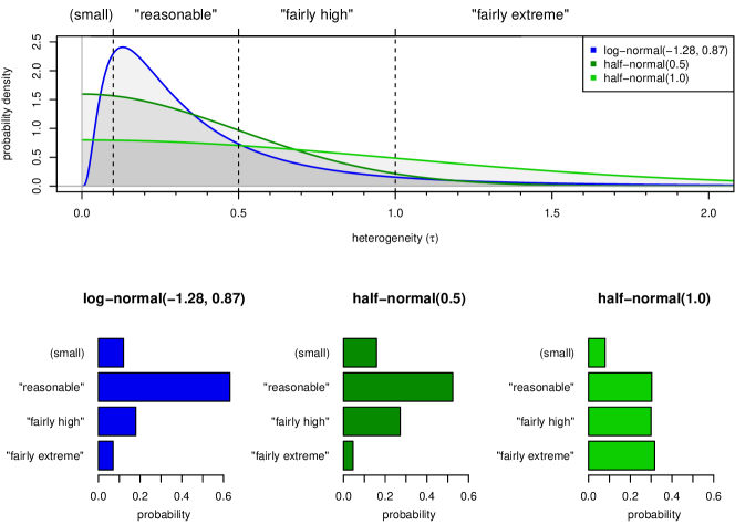
Figure 3: Comparison of the heterogeneity prior proposed by Turner et al. (2015)⁷⁵ for log-ORs in a general setting (a log-normal distribution with $\mu\!=\!-1.28$ and $\sigma\!=\!0.87$, shown in blue) with half-normal priors (with scales 0.5 and 1.0). The bottom plots especially contrast the implied prior probabilities for the heterogeneity categories proposed by Spiegelhalter et al. (2004)¹⁵ Sec. 5.7 (see also Tables 2 and 3).

The heterogeneity categories from Table 2 are marked, and at the bottom, the probabilities for the categories are shown. The probabilities assigned by the half-normal(0.5) prior and the “empirical” prior are roughly in agreement, while the half-normal(1.0) prior would assign more or less equal probabilities to the “reasonable”, “fairly high” and “fairly extreme” categories, and leave only $8\%$ probability for smaller values. Similar arguments hold also for other log-transformed effect scales.

4.4 Regression slopes

Very closely related to mean differences is the more general case of meta-analysis of regression parameters (slopes or interactions) and their standard errors.⁹³ In the special case of a single binary covariate, the regression effectively reduces to a two-group comparison, and consideration of additional covariates then may allow for some “adjustment”. When the covariate is continuous, however, extra care needs to be taken, since not only the endpoint’s scaling is relevant (the regression’s “$y$ variable”), but also the regressor’s scaling (the regression’s “$x$ variable”). Whether the regressor is expressed in, say, days or weeks, affects the resulting slope parameter (and its standard error) by a corresponding re-scaling by a factor of seven. The regressor’s scaling will then similarly also affect the scale of the anticipated heterogeneity: when combining estimated (linear) regression coefficients, which are to be interpreted as “the expected change in $y$ for a one-unit change in $x$”, the heterogeneity between estimates depends on the units of $x$. For example, the variability expected among temporal changes that are expressed on a per-week scale rather than a per-day scale should be seven times as large.

The immediate question then is what increment in the regressor to base heterogeneity considerations on; what is eventually needed is a statement of the form “for a change in the regressor by a difference of $\Delta_{x}$, the associated effects are anticipated to vary by a magnitude of $\tau$”, and that difference $\Delta_{x}$ needs to be specified. Sometimes there may be obvious “natural” units to be used, for example in the common case of a binary (zero/one) coded covariate (e.g. for treatment vs. control or males vs. females); the obvious difference to consider here is an increment of $\Delta_{x}=1$. Otherwise the width of the regressor’s distribution may be relevant.⁹⁴ Consider again the case of a binary covariate and a balanced setup; the standard deviation of the binary variable will then be $\frac{1}{2}$, so that twice the standard deviation might generally be a sensible scale to consider. Note though that this is by no means universally applicable, as such scales may be affected by many factors (e.g., inclusion criteria in clinical trials) and might also be very different between studies. Note that the $\Delta_{x}$ value needs to be the same across the considered studies.

Once the “reference” increment $\Delta_{x}$ has been determined, a prior for the associated heterogeneity may be formulated. In case the actual analysis then is done with respect to a differing scaling, the prior needs to be re-scaled accordingly. For example, if a prior with scale $s$ was determined for a per-week increment, but the actual analysis is based on the per-day regression coefficients, then their prior should have scale $\frac{s}{7}$. The UISD $\sigma_{\mathbb{1}}$ then also scales proportionally.

Note that the above arguments extend beyond simple linear regressions with continuous outcomes, for example, logistic regressions, Poisson regressions or survival analyses, in which regression parameters then relate to log-ORs, log-IRRs or log-HRs. Once a reference increment $\Delta_{x}$ has been determined, the arguments regarding log-transformed endpoints discussed earlier in Section 4.3 apply, and potential re-scaling issues still need to be considered. A way to circumvent considerations of regressor’s or response’s scales may be to move to standardized regression coefficients instead, which are unitless and are somewhat similar to SMDs (see also Section 4.2) or correlations (see Section 4.5).⁸⁸. Depending on the exact type of regression analysis and the standardization technique (e.g., in case of a logistic regression, and when standardization is done based only on the regressor’s scale),⁹⁵, ⁹⁶, ⁹⁷ arguments relevant for log-transformed endpoints might also apply.

4.5 Correlation coefficients

Estimated correlation coefficients (Pearson’s $r$) are commonly quoted and summarized for studies dealing with paired observations.³, ⁴, ⁹⁸ Correlation coefficients are restricted to the domain $[-1,\,1]$, with values of $|r|=1$ indicating perfectly linear (positive or negative) correlation, and $r=0$ indicating uncorrelatedness.⁹⁹ Due to the problems with bounded parameter spaces, correlation coefficients are commonly analyzed after an appropriate transformation using Fisher’s $z$ transform, which is defined as $z_{i}=\frac{1}{2}\log\Bigl{(}\frac{1+r_{i}}{1-r_{i}}\Bigr{)}=\mathrm{arctanh}(r_{i})$. This transformation maps the original domain to the real line, and in particular, it is also a variance stabilizing transformation; the (approximate) standard error of the transformed $z_{i}$ value only depends on the $i$th study’s sample size $n_{i}$ and is given by $\frac{1}{\sqrt{n_{i}-3}}$. Correlation values within the range $-0.5<r_{i}<0.5$ are little affected by the transformation, which makes more of a difference for more extreme values.

An upper limit to the expected heterogeneity may be specified by considering a uniform distribution of $\theta_{i}$ values across the range of correlation coefficients as a “worst case”. For plain (correlation $r$) values, this would imply a variance of $\frac{1}{3}=0.58^{2}$. On the scale of $z$-transformed values, this implies a distribution with probability density function $p(z)=\frac{2}{(\exp(-z)+exp(z))^{2}}$, that has a zero mean and a variance of $\frac{\pi^{2}}{12}\approx 0.91^{2}$ (these moments might actually motivate a prior for the overall effect $\mu$, too). The standard error of $z_{i}$ values after transformation (see above) implies a UISD of approximately $\sigma_{\mathbb{1}}=1.0$. With that, it should usually be safe to expect heterogeneity values well below $\tau=1.0$.

If $\tau$ values near unity (or $0.91$) already imply rather extreme heterogeneity, the question remains what constitutes “large”, yet reasonable heterogeneity. For that, we may consider the somewhat more moderate cases of $r\sim\mathrm{Uniform}(-0.5,0.5)$ or $r\sim\mathrm{Uniform}(0.0,0.8)$. Both these cases happen to lead to similar variances of $\mathrm{Var}(z)=0.30^{2}$ on the transformed scale, so that $\tau=0.30$ may already be considered “large” heterogeneity.

While the use of “plain”, un-transformed correlation values within the NNHM framework is a bit problematic due to the bounded parameter space that is not reflected in the model, it is not uncommon. We have already seen some hints of what amounts of between-study variance for plain correlations may be possible or plausible in the considerations above; a value of $\tau=\frac{1}{\sqrt{3}}=0.58$ (corresponding to a uniform distribution in $r$) would already be extreme; one would most likely expect values way less than even half as much.

Van Erp et al. (2017)⁸² collected heterogeneity estimates reported in studies that were published in the Psychological Bulletin. Although the figures were not identified as being based on Fisher-$z$ transformation or not (apparently a mix of both was encountered), these numbers may provide some empirical motivation. Among the observed heterogeneity estimates for correlation endpoints in 539 analyses from 25 studies, a median and 95% quantile of 0.12 and 0.29, respectively, were found. Similarly, Steel et al. (2015)⁸¹ quote heterogeneity estimates from 292 management-related meta-analyses in the range of 0.0 to 0.4, with a median of 0.16.

5 Example applications

5.1 Mean differences

Grande et al. (2015)¹⁰⁰ Analysis 1.5 investigated the effect of physical exercise (vs. no exercise as control) on the duration of acute respiratory infections (ARIs). Four studies were jointly considered in a meta-analysis, the endpoint of interest was the mean difference in the number of symptom days per episode. The relevant data are shown in Table 7.

Table 7: Mean difference (MD) example data due to Grande et al. (2015).¹⁰⁰ $\bar{x}$, $s$ and $n$ denote the treatment and control groups’ empirical means, standard deviations and sample sizes. The $y_{i}$ are the derived MDs and $\sigma_{i}$ the associated standard errors that eventually go into the analysis (see Section 2.1). Here, mean differences are on the scale of days (change in disease duration). Negative estimates $y_{i}$ indicate a beneficial effect.

		treatment group			control group			MD
$i$	study	$\bar{x}_{1;i}$	$s_{1;i}$	$n_{1;i}$	$\bar{x}_{2;i}$	$s_{2;i}$	$n_{2;i}$	$y_{i}$	$\sigma_{i}$
1	Nieman (1990)	3.60	2.97	18	07.00	5.94	18	-3.40	1.57
2	Çiloğlu (2005)	5.15	1.56	60	06.10	1.00	30	-0.95	0.27
3	Barrett (2012)	9.30	5.13	47	11.40	5.75	51	-2.10	1.10
4	Sloan (2013)	5.30	1.50	16	06.30	2.20	16	-1.00	0.67

The outcome here is measured in units of days (change in symptom duration for treated patients relative to the control group). For the purpose of the present analysis, ARIs were defined as “infections of the respiratory tract that last for less than 30 days”,¹⁰⁰ while ARI durations generally are substantially shorter, lasting of the order of a week.¹⁰¹, ¹⁰² With that, the reduction in symptom days cannot be more than (roughly) a week. ARIs may be caused by bacterial or viral pathogens; the effect of antibiotic treatment is in a shortening of the order of one day.¹⁰³ From the data (Table 7), we can derive estimates of the UISD, which here is at an average of $s_{\mathbb{1}}=3.9$.

The treatment effect may be expected to be of the order of days (anything below 1 day would probably not be considered clinically meaningful), and a similar magnitude may be expected for the heterogeneity. Values $\tau>1$ would make the between-study heterogeneity larger than the effect of antibiotics, which seems implausible. Variations in treatment effects of the order of several days would probably imply that the effect was several times larger in some studies than in others.

A $\tau$ value of $1.0$ would imply a median difference in true effects of $\approx 1$ day for a random pair of studies (see Table 1), which might be at the upper end of the plausible range. A half-normal(0.5) prior would imply $\mathrm{P}(\tau\leq 1)\approx 95\%$, and considering the corresponding prior predictive distribution (see Table 3), we can see that this implies a 95% prior predictive interval of roughly $\pm 1$ day around the overall mean effect.

For the present example, we would hence suggest a half-normal(0.5) prior. Note that this is a common, well-researched condition. For more uncertain cases, one might want to go for a heavier-tailed prior. A meta-analysis based on the half-normal(0.5) prior is illustrated in Figure 4. Among the four studies considered, one suggests a stronger effect than the others, however, due to its relatively small size and correspondingly large associated standard error, it is still consistent with the remaining three. The estimated heterogeneity (the median and 95% credible interval (CI) are shown in the bottom left of the forest plot) here has barely changed from the a priori anticipated amount (see Table 3). The heterogeneity’s posterior is also illustrated in Figure 8; prior and posterior are very similar in this case. The resulting combined estimate then also suggests a more moderate effect, namely, a reduction of the order of one symptom day, with an uncertainty of about a factor of two. The estimated heterogeneity is relatively low compared to the width of the overall mean’s CI, and so the prediction interval is only slightly longer, and the shrinkage intervals show substantially greater precision than the original estimates. Sensitivity to other prior choices is also investigated for this example in Appendix D.4.

5.2 Standardized mean differences

Aalbers et al. (2017)¹⁰⁴ Analysis 1.1 investigated the short-term effect of music therapy on depression symptoms; four studies comparing music therapy plus treatment-as-usual (TAU) versus TAU alone were found. Within these four studies, differing clinician-rated symptom scores were utilized in order to quantify depression severity: the Hamilton rating scale for depression (HAM-D), considering potentially differing numbers of items between studies, as well as the Montgomery-Åsberg depression rating scale (MADRS). In order to facilitate a joint analysis, the meta-analysis was based on SMDs (here: Hedges’ $g$); the relevant data are shown in Table 8.

Table 8: Standardized mean difference (SMD) example data due to Aalbers et al. (2017).¹⁰⁴ $\bar{x}$, $s$ and $n$ denote the treatment and control groups’ empirical means, standard deviations and sample sizes. The $y_{i}$ are the derived SMDs and $\sigma_{i}$ the associated standard errors that eventually go into the analysis (see Section 2.1). The original data are based on different depression symptom scores that are measured on different scales. Negative estimates $y_{i}$ indicate a reduction in symptom severity.

		treatment group			control group			SMD
$i$	study	$\bar{x}_{1;i}$	$s_{1;i}$	$n_{1;i}$	$\bar{x}_{2;i}$	$s_{2;i}$	$n_{2;i}$	$y_{i}$	$\sigma_{i}$
1	Chen (1992)	-98.23	15.19	34	-67.06	15.19	34	-2.03	0.30
2	Radulovic (1996)	-16.50	10.00	30	-10.60	10.00	30	-0.58	0.26
3	Albornoz (2011)	0-8.17	05.89	12	0-3.83	05.31	12	-0.75	0.42
4	Erkkilä (2011)	-10.70	08.40	30	0-6.05	08.06	37	-0.56	0.25

The outcome measured on the SMD scale means that a unit change in $y_{i}$ corresponds to a one standard deviation change in the symptom severity score. Considering e.g. the Albornoz (1992) study,¹⁰⁵ which was measuring change in symptom severity using the 17-item HAM-D scale with a within-group standard deviation of about 5 (see Table 8), a difference of 1 on the SMD scale here would roughly correspond to a 5-point change in HAM-D score.¹⁰⁶, ¹⁰⁷, ¹⁰⁸, ¹⁰⁹ In terms of SMD, this would already be considered a “large” effect.⁸⁹, ⁹⁰ The UISD for SMDs is predicted at $\sigma_{\mathbb{1}}=2$, while from the present data here we get a very similar empirical average of $s_{\mathbb{1}}=2.2$.

For the between-study differences, we would assume that they would be mostly in the “small” to “medium” range ($\ll 1$) — otherwise effects would be differing by a standard deviation or more between studies, and also the studies’ confidence intervals (which are roughly of the size $\sigma_{i}\approx\frac{\sigma_{\mathbb{1}}}{\sqrt{n_{i}}}=\frac{2}{\sqrt{n_{i}}}$) would be unlikely to have any overlap. Rhodes et al. (2015)⁷⁴ in their empirical investigation based on the Cochrane Database of Systematic Reviews predicted a median and 95% quantile of 0.18 and 2.43 for the heterogeneity $\tau$ (where the large upper quantile appears rather extreme, based on the above arguments). Similarly, van Erp et al (2017)⁸² inferred a median and 95% quantile of 0.20 and 0.66, respectively, based on heterogeneity estimates within a smaller data base.

A value of $\tau=1.0$ would imply a median difference of $\approx 0.95$ (“large”) for a random pair of true study means $\theta_{i}$ (see Table 1), which already appears like a rather extreme amount; values of $\tau=0.5$ (implying mostly “medium” sized between-study differences) or below seem to be more plausible. A half-normal(0.5) prior would cover this range and would imply a prior median (for $\tau$) slightly above the magnitude suggested the empirical investigations (see also Table 3).

       

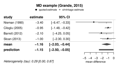
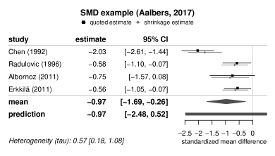
Figure 4: Forest plots for the two examples discussed in Sections 5.1 and 5.2. In both cases, a half-normal(0.5) prior for the heterogeneity $\tau$ was used. Besides the intervals based on the quoted estimates, the shrinkage intervals are shown in grey. At the bottom, the credible interval for the overall mean ($\mu$) is shown along with the prediction interval for a “new” additional study effect $\theta_{k+1}$. The estimated heterogeneity ($\tau$) is quoted in terms of the posterior median and shortest 95% credible interval.

For the present example, we would then suggest a half-normal(0.5) prior as a slightly conservative choice, in order to reflect the potential heavy-tailedness suggested by Rhodes et al. (2015),⁷⁴ and to account for the fact that the empirical data might be of limited relevance for the present example data. A meta-analysis based on the half-normal(0.5) prior is illustrated in Figure 4. Among the four studies, three consistently indicate estimates in the range $0.5$ – $0.8$, while the first one shows a huge effect estimate of the order of $2.0$; a positive amount of heterogeneity appears to be present (the CI for $\tau$ is in a strictly positive range; see also Figure 8), and the eventual combined estimate indicates a “small” to “very large” average effect. Given the pronounced heterogeneity one might discuss whether the estimation of a pooled effect is meaningful. Nevertheless, we use this example to illustrate the use of Bayesian methods in heterogeneous situations, where heterogeneity cannot be explained and good reasons are available to perfom a quantitative meta-analysis despite of large heterogeneity. The large estimated heterogeneity here results in a wide CI for the overall effect, a very wide prediction interval, and also very little shrinkage for the estimated study-specific effects $\theta_{i}$.

5.3 Log-transformed effect scales

5.3.1 Log odds ratio

A systematic review was performed by Crins et al. (2014)¹¹⁰ to investigate the effect of Interleukin-2 receptor antagonists (IL2-RA) on recovery of pediatric patients following liver transplantation. One aspect of interest was the occurrence of acute rejection (AR) reactions as a common adverse event. Two randomized controlled trials reporting such data were found, the event counts along with the corresponding (logarithmic) odds ratios and standard errors are shown in Table 9. Both studies indicated a reduction in the chances of an AR event for the treatment group.

Table 9: Log-OR example data.¹¹⁰ $a$ and $n_{1}$ as well as $c$ and $n_{2}$ denote the event counts and total numbers of patients in treatment and control groups, which together summarize the trial outcome in terms of a $2\!\times\!2$ table. The $y_{i}$ are the derived logarithmic odds ratios and $\sigma_{i}$ are the associated standard errors that eventually go into the analysis (see Section 2.1). Negative values here indicate a reduction of the event odds, i.e., a beneficial treatment effect.

		treatment group		control group		log-OR
$i$	study	events ($a_{i}$)	total ($n_{1;i}$)	events ($c_{i}$)	total ($n_{2;i}$)	$y_{i}$	$\sigma_{i}$
1	Heffron (2003)	14	61	15	20	-2.31	0.60
2	Spada (2006)	04	36	11	36	-1.26	0.64

The treatment effect is expressed and analyzed on a logarithmic scale here. A heterogeneity magnitude of $\tau=1.0$ would imply that any random pair of studies would be expected to exhibit effects differing by a factor of 2.6 (see Table 1), which seems quite extreme already; values like $\tau=0.5$ or below seem more plausible. In a simular investigation involving 14 studies and based on adult patients (Goralczyk et al.; 2011),¹¹¹ a mean treatment effect (log-OR) of $-0.26$, corresponding to an OR of $0.77$, was found. The UISD for a log-OR is at $\sigma_{\mathbb{1}}\approx 4$ per subject, while for the present data here we get an estimate of $s_{\mathbb{1}}=5.4$. An empirical study based on a large number of meta-analyses predicts a median (95% quantile) of 0.28 (1.16) for the heterogeneity (Turner et al.; 2015),⁷⁵ and an investigation of heterogeneity estimates found a median (95% quantile) of 0.00 (1.05) (Günhan et al.; 2020).⁸⁵ In the data from the closely related meta-analysis by Goralczyk et al. (2011),¹¹¹ the heterogeneity is estimated at 0.12 (0.38).

A half-normal(0.5) prior would mostly cover values $\tau<1.0$ (up to “fairly high” heterogeneity according to Table 2) with an expectation and median below $0.5$ (see also Table 3). The resulting 95% prior predictive interval would still include effects within a factor of $3$ around the overall mean log-OR $\mu$. For the present investigation, we would then suggest a half-normal(0.5) prior as a reasonably conservative choice, which also agrees roughly with the empirical evidence (see Fig. 3). A meta-analysis based on this prior is shown in Figure 5. In this example we have two studies only, demonstrating the somewhat speculative nature of infering heterogeneity based on sparse data, and higlighting the value of considering a-priori probabilities. In the present case, the two studies involved are not very large, and their resulting CIs are overlapping, which makes the data consistent with a wide range of heterogeneity values, from homogeneity ($\tau\!=\!0$) up to magnitudes of $\tau\!=\!10$ or $\tau\!=\!20$. Including the weakly informative heterogeneity prior, and effectively down-weighting unreasonably large heterogeneity values, then leads to an estimate of $-1.81$ for the log-OR, corresponding to a reduction in the odds of an AR event down to $\exp(-1.81)=16\%$. While the uncertainty still is large (ranging roughly from $5\%$ up to $50\%$), the analysis clearly indicates a substantial reduction in AR events here. The heterogeneity’s posterior density is also shown in Figure 8; here we can see that for the present example constellation, the posterior is very similar to the prior. With the very uncertain original estimates (due to the small sample sizes), the overall mean’s CI is wide, but the additional width of the prediction interval is limited due to the (prior and empirical) information on the heterogeneity, and a noticeable shrinkage effect is also observable.

5.3.2 Log incidence rate ratio

Four studies investigating the effect of ferric carboxymaltose vs. placebo in heart-failure patients with iron deficiency were jointly analyzed by Anker et al. (2018).¹¹² The main outcome was the incidence rate ratio (IRR) with respect to the composite endpoint of recurrent cardiovascular (CV) hospitalisations or CV death. The relevant available data are shown in Table 10. The eventual analysis is based on the logarithmic ratio of the event rates (per 100 patient-years of follow-up) of treatment over placebo group.

Table 10: Log-IRR example data.¹¹² The incidence rate ratios for the composite endpoint of recurrent cardiovascular (CV) hospitalisations and CV mortality are given for each study. For the analysis, the logarithmic rate ratio is considered. Negative values here indicate a reduction of incidence rates, i.e., a beneficial treatment effect.

				log-IRR
$i$	study	rate ratio [95% CI]	$n_{i}$	$y_{i}$	$\sigma_{i}$
1	Fair-HF (2009)	0.44 [0.22, 0.90]	459	-0.82	0.36
2	Confirm-HF (2015)	0.68 [0.38, 1.21]	301	-0.39	0.30
3	Efficacy-HF (2015)	1.09 [0.21, 5.54]	034	0.09	0.83
4	Fer-Cars-01 (2018)	0.87 [0.07, 10.4]	045	-0.14	1.28

As in the previous example, the outcome is analyzed on the logarithmic scale, so that many arguments apply essentially analogously here. Regarding empirical evidence on previously encountered amounts of heterogeneity, there are no studies available that would be directly applicable for log-IRRs, however, odds ratios and rate ratios have quite some similarity, so that these findings also have some bearing here. The UISD here is at $\sigma_{\mathbb{1}}=2$ per event (see Appendix A.3); with a total of 114 events observed among a total of 839 patients¹¹² Tab. 4 (a rate of $\approx 0.14$ events per patient), this would correspond to $\sigma_{\mathbb{1}}\approx\frac{2}{\sqrt{0.14}}=5.4$ per patient. For the present data, we empirically get an average of $s_{\mathbb{1}}=6.6$.

       

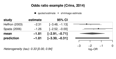
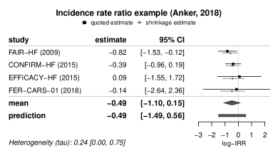
Figure 5: Forest plots for the two examples discussed in Sections 5.3.1 and 5.3.2. In both cases, a half-normal(0.5) prior for the heterogeneity $\tau$ was used.

For this example, we would again suggest a half-normal(0.5) prior. A meta-analysis based on this prior is shown in Figure 5. While the data look homogeneous (all intervals have some overlap, also because some studies are very small and intervals are correspondingly wide), we would still anticipate the possibility of heterogeneity — since from experience we know that heterogeneity is frequently present, and because we know that heterogeneous circumstances are still likely to produce data that may still “look homogeneous”.⁷ Compared to our a-priori expectations of $\tau$ values up to $0.98$ (see Table 3), the posterior then suggests a slightly lower heterogeneity range of up to $0.75$, but the data do not provide very much evidence in this regard (see also the posterior in Figure 8). The mean treatment effect eventually is at a log-IRR of $-0.49$, corresponding to an IRR of 61% (i.e., a reduction in the event rate), with a CI ranging from 33% up to 116%. For these somewhat homogeneous estimates, one can see that the ones with very large associated standard errors eventually have shrinkage estimates close to the overall prediction interval. A sensitivity analysis investigating alternative prior choices for this example is also shown in Appendix D.4.

5.3.3 Log odds

Neuenschwander et al. investigated the use of historical data in order to inform the analysis of a new data set.⁷⁷ A meta-analysis of several trials in ulcerative colitis was performed in order to support the analysis of a subsequent phase II trial. The figure of interest here was the probability for clinical remission at week 8 in placebo-treated patients, and the main interest was in a prediction for the new study’s event probability, to then formally integrate this in a subsequent analysis using a meta-analytic-predictive (MAP) approach.⁷² Four previous randomized controlled trials reporting this endpoint were available, their data are shown in Table 11.

Table 11: Log-odds example data due to Neuenschwander et al. (2010).⁷⁷ The $n_{i}$ and $x_{i}$ here denote total numbers and the numbers of remitting patients among these. Analysis is done based on the derived log-odds $y_{i}$ and their standard errors $\sigma_{i}$.

		remission		proportion	odds	log-odds
$i$	study	events ($x_{i}$)	total ($n_{i}$)	$p_{i}=\frac{x_{i}}{n_{i}}$	$\frac{x_{i}}{n_{i}-x_{i}}=\frac{p_{i}}{1-p_{i}}$	$y_{i}$	$\sigma_{i}$
1	Feagan (2005)	09	063	0.143	0.167	$-1.79$	$0.36$
2	Rutgeerts (2005a)	18	121	0.149	0.175	$-1.74$	$0.26$
3	Rutgeerts (2005b)	07	123	0.057	0.060	$-2.81$	$0.39$
4	Van Assche (2006)	06	056	0.107	0.120	$-2.12$	$0.43$

Instead of working directly on the estimated probabilities $p$, the analysis here is done based on the odds $\frac{p}{1-p}$, and a subsequent log-transformation.⁹²

Homogeneity of placebo rates is not expected — differences between control rates are among the main reasons for requiring a control arm for each RCT, and for pursuing a contrast-based analysis.¹¹³, ¹¹⁴ The studies were designed aiming for an estimate of the treatment effect, and the placebo rate originally way mostly a nuisance parameter here. However, some amount of similarity still is anticipated, and the aim of this exercise is to carefully derive the predictive distribution, which of course depends on the amount of heterogeneity $\tau$.

The earliest of the four studies was planned anticipating a remission rate of 10% for the placebo group,¹¹⁵ and hence a UISD of $\sigma_{\mathbb{1}}\approx\sqrt{\frac{1}{0.1}+\frac{1}{0.9}}=3.33$ may be expected. Empirically, we get an estimate of $s_{\mathbb{1}}=3.2$ from the present data set.

As the endpoint are logarithmic odds, we may again apply similar reasoning as in the previous subsections, regarding the anticipated ratios of odds. However, a major difference here is that while clinical trials are usually carefully designed to provide reliable estimates of treatment effects (treatment/control contrasts), this is not necessarily the case for the event rates that we are considering here; we may expect the log-odds to be more variable than the log-ORs. With this in mind, and considering conservatism and robustness particularly desirable in the present context, we would suggest a half-normal(1.0) prior here. From Table 3, we can see that the implied 95% prior predictive interval then spans a range of roughly a factor 9 around the median $\mu$. Given the context, it may be of particular interest to consider the associated prior maximum sample size $n^{\star}_{\infty}$ (see Section 3.4.5); for the prior median of $\tau=0.67$, we have $\frac{\tau}{\sigma_{\mathbb{1}}}=\frac{0.67}{3.2}=0.21$, corresponding to a maximum size of $n^{\star}_{\infty}=23$ (compared to an original total of 363 subjects included in the analysis). The prior’s 95 % quantile is (approximately) at $\tau=2$, and larger values would effectively imply (with $n^{\star}_{\infty}<3$) an almost noninformative posterior predictive distribution.

The eventual analysis is illustrated in Figure 6. Looking at the heterogeneity’s posterior (Figure 8), one can see that heterogeneity here appeared to be less than anticipated. The prediction interval is relatively wide, and on the back-transformed scale is centered at a probability of 0.11 with its 95% posterior predictive interval ranging from 0.03 to 0.34. The posterior predictive distribution’s standard error is 0.70, and relative to the UISD, this roughly corresponds to an effective sample size of $\frac{3.2^{2}}{0.70^{2}}=21$ subjects.

5.4 Regression slopes

Bergau et al. (2017)¹¹⁶ investigated predictors of all-cause mortality among patients with an implantable cardioverter-defibrillator (ICD) device. Several potential covariables were considered, among these the left ventricular ejection fraction (LVEF), which is a measure of the efficiency of heart function that is usually determined via echocardiography. LVEF is commonly expressed in percent, where 52%–72% are normally observed in healthy individuals, while values below 30% are considered abnormal.¹¹⁷ Criteria for an indicated ICD therapy include various conditions, including thresholds on the LVEF in the range 30–40%.¹¹⁸. Five studies were found that had reported on survival analyses including LVEF as a predictor, and a meta-analysis was performed based on the coefficients standardized to a 5 percentage point decrease in LVEF; the data are shown in Table 12. The different studies also included different sets of additional covariates in their analyses.¹¹⁶

Table 12: Regression example data.¹¹⁶ Regression slopes result from survival analyses and are expressed in terms of hazard ratios (HRs) and with reference to a 5 percentage point decrease in LVEF. The baseline means and standard deviations of LVEF values are also shown.

		LVEF (%)				log-HR
$i$	study	mean	s.d.	HR [95% CI]	$n_{i}$	$y_{i}$	$\sigma_{i}$
1	Maciąg (2012)	28.0	04.0	1.16 [0.90, 1.51]	0121	0.148	0.132
2	Hage (2013)	28.0	15.0	1.23 [1.08, 1.40]	0696	0.207	0.066
3	Demirel (2014)	31.9	09.3	1.29 [1.02, 1.64]	0099	0.255	0.121
4	Konstantino (2016)	31.6	11.1	1.16 [1.02, 1.32]	1125	0.148	0.066
5	Rodríguez-Mañero (2016)	26.2	07.6	1.23 [1.10, 1.36]	1174	0.207	0.054

The regressor, LVEF, here is expressed in percentages (between 0 and 100), which might just as well have been expressed as a fraction (between 0 and 1), while for the analysis a unit of a 5 percentage point decrease was used — this highlights the importance of clarifying the scale of the increment $\Delta_{x}$ that heterogeneity considerations are to be based on. Table 12 also shows the distributions of LVEF within studies; these are roughly similar and have standard deviations of the order of 10 percentage points. For the “reference” increment $\Delta_{x}$ for judging plausible heterogeneity magnitudes, we will then consider a difference of 20 percentage points, which roughly spans the bulk of LVEF values encountered in each of the studies. This also coincides with the range of values considered “normal” (52%–72%) or the difference between “normal” and “abnormal” ranges ($\geq 52\%$ vs. $<30\%$) here. The (empirical) UISD for the present data is at $s_{\mathbb{1}}=1.9$ (for the 5% increments shown in Table 12, corresponding to $s_{\mathbb{1}}=7.5$ for a 20% difference).

Since the regression coefficient is to be interpreted as a logarithmic HR, we will assume a half-normal(0.5) prior for the effect correponding to a $\Delta_{x}=20$ percentage point increment (analogously to the arguments made in Sections 5.3.1 and 5.3.2). For the 5 percentage point decreases considered in the analyses, this then implies a four-fold smaller heterogeneity, i.e., a half-normal(0.125) prior. Analysis results for a half-normal(0.125) prior are illustrated in Figure 6.

       

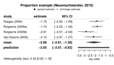
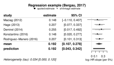
Figure 6: Forest plots for the examples discussed in Sections 5.3.3 and 5.4. For the log-odds, a half-normal(1.0) prior was used, and for the log-HR regression slopes, a half-normal(0.125) prior was used for the heterogeneity $\tau$.

The estimates are very homogeneous, which is evident from the forest plot as well as from the estimated heterogeneity (see also Figure 8). The overall log-HR estimate is at 0.19, corresponding to 1.21-fold increased mortality hazard for a 5 percentage point decrease (worsening) in LVEF.

5.5 Correlations

Molloy et al. (2014)¹¹⁹ investigated the relationship between conscientiousness and medication adherence. A total of 16 relevant studies reporting correlation coefficients of the two factors were found, which were also graded according to their methodological quality. Three of the studies were rated with the highest quality score; their data are shown in Table 13. The data are also available as part of the metafor R package.⁹¹ In order to avoid problems due to the bounded parameter space of correlations $r_{i}$ (between $-1$ and $+1$), we will use the Fisher-$z$ transformed values instead. Note that, since in the present example the reported correlations ($r_{u}$) are relatively close to zero, the corresponding Fisher-$z$ values ($y_{i}$) are almost identical here (see Table 13; $r_{i}$ and $y_{i}$ values only differ in their third decimal place) and the transformation eventually makes little difference.

Table 13: Correlation example data.⁹¹, ¹¹⁹ $r_{i}$ and $n_{i}$ here denote the empirical correlation coefficients and the underlying sample sizes. The $y_{i}$ are the Fisher-$z$ transformed correlations and $\sigma_{i}$ the associated standard errors that eventually go into the analysis (see Section 2.1). A positive effect size $y_{i}$ here indicates a positive correlation.

				Fisher’s $z$
$i$	study	Correlation $r_{i}$	$n_{i}$	$y_{i}$	$\sigma_{i}$
1	Stilley (2004)	0.24	158	0.245	0.080
2	Ediger (2007)	0.05	326	0.050	0.056
3	Jerant (2011)	0.01	771	0.010	0.036

As elaborated in Section 4.5, we expect smaller magnitudes of heterogeneity for correlation endpoints (say, mostly $\tau\leq 0.3$); the UISD is at $\sigma_{\mathbb{1}}=1.0$, which also matches the figures we see empirically in the present data set ($s_{\mathbb{1}}=1.004$). Van Erp et al. (2017)⁸² report a median and 95% quantile of 0.12 and 0.29, respectively, for empirically observed heterogeneity estimates from published studies. Meta-analysing the remaining set of 13 studies from the present data set¹¹⁹ (using a uniform prior), in order to quantify the evidence “external” to the example data, yields a heterogeneity estimate of 0.07 with 95% CI [0.00, 0.17].

Heterogeneity values of $\tau=0.1$ or $\tau=0.2$ would imply differences between a random pair of studies of a similar order of magnitude (see Table 1). A half-normal(0.2) prior for the heterogeneity would cover values mostly in the range below $0.4$, with a prior median at $\tau=0.13$ (see Table 3).

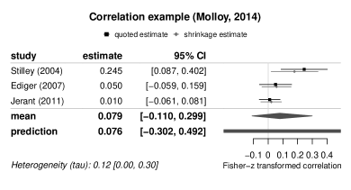
Figure 7: Forest plot for the example discussed in Section 5.5. For the (Fisher-$z$ transformed) correlations, a half-normal(0.2) prior was used for the heterogeneity $\tau$.

For the present analysis, we would then suggest a half-normal(0.2) prior for the heterogeneity. A meta-analysis of the example data based on this prior is illustrated in Figure 7. The two traits were originally measured using differing scales, so that complete homogeneity might be considered especially unlikely. The heterogeneity’s resulting posterior median is at $\tau=0.12$ (with the 95% CI ranging up to 0.30), its posterior distribution is also illustrated in Figure 8. The three studies are of differing size and suggest neutral to slightly positive correlation between conscientiousness and medication adherence. The resulting mean estimate is positive at about 0.08, while the CI ranges from negative to positive ($-0.1$ to $+0.3$).

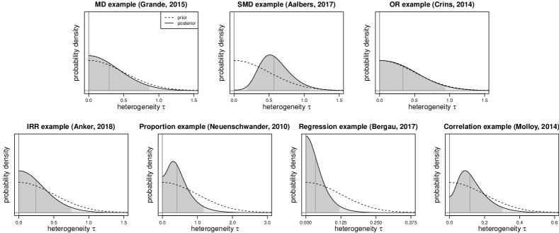
Figure 8: Marginal prior and posterior densities for the heterogeneity parameter $\tau$ in the seven examples discussed in Section 5. The dashed lines show the prior densities, the solid lines show the posteriors. The area shaded in dark grey indicates the 95% credible interval, the vertical line is the posterior median.

6 Discussion

While executing a Bayesian meta-analysis is not technically difficult, specifying a widely acceptable prior remains a challenge, especially when it comes to the heterogeneity parameter $\tau$. Although the problem may appear complex at first, it is usually possible to break down the specification into a number of more specific questions that are easier to approach one-by-one. These steps are summarized in Table 6 and may be outlined as follows: (i) what is the effect’s scale? (ii) what is the probable magnitude of other effects? (iii) how large is the unit information standard deviation (UISD)? (iv) is relevant empirical information available? The information may then be related to more concrete prior specifications by constraining (v) prior quantiles (of $\tau$) (vi) prior predictive quantiles (of $\theta_{i}$), and (vii) other prior properties. We have demonstrated the prior specification in seven applications involving few studies and covering a range of common effect scales and application areas, leading to sensible prior distributions and results in all examples. Besides the case of few studies, another context in which (weakly) informative priors are useful is whenever marginal likelihoods (or Bayes factors) need to be computed.⁷³ Calculation of marginal likelihoods requires proper prior distributions, and special care must be taken in their selection in order to avoid (seemingly) paradoxical results.¹, ¹²⁰

In many applications, the results will be robust to variations of the prior, which may also be checked in sensitivity analyses. The prior specification will usually not be the most crucial or influential among the line of assumptions being made, which include normality,⁵ exchangeability, the selection of estimates to be pooled, or the choice between effect measures.¹²¹ Different prior specifications will of course leave their imprint on the posterior distribution, for example, results based on short- or heavy-tailed priors will reflect the differing assumptions, which may be based on emphasizing regularisation or robustness aspects. There usually is no unique “correct” prior, and “sceptical” or “enthusiastic” results may be derived by implementing corresponding prior assumptions.⁴² Even uncertainty in the prior distribution itself (or its scale) may be accommodated by using mixture priors. Consideration of the stochastic ordering of heterogeneity priors may help assessing more or less conservative settings, which may be useful for the definition of sensitivity analyses. However, we would also like to warn against inflationary default specification and execution of multiple analyses here, as the resulting alternative estimates may lead to unnecessary ambiguity or inconsistent (flip-flopping) conclusions. In Appendix D.4, sensitivity analyses are discussed in the context of the two examples from Sections 5.1 and 5.3.2. Pre-specification of analyses (and their intended consequences) may help here. In case there is genuine a-priori uncertainty about the heterogeneity’s magnitude, this might better be reflected in a single prior (e.g., in terms of a mixture distribution). Either way, one needs to be prepared and willing to base the eventual analysis results on the posterior also when the data have little information on heterogeneity to add to the weakly informative prior, as was the case for some of the examples discussed here (see Figure 8). If it is not possible to specify a suitable (weakly) informative prior for the expected heterogeneity, then one might have to resort to a more conservative approach using uninformative priors.

Another central assumption crucial to the validity of inference is the exchangeability (see Section 2.1). This might be compromised by selection effects, for example, publication bias¹²² or reporting bias.¹²³ Especially in the case of only few studies, such effects might be hard to detect from the data, and information on the presence of selection effects may need to come from considerations of the context.

Choice of heterogeneity priors has consequences for estimation of the overall mean parameter, but in particular also in prediction and shrinkage applications, as the inferred heterogeneity directly impacts on the amount of borrowing-of-strength;²⁰, ³³, ⁷² smaller heterogeneity will lead to stronger pooling of estimates, and larger heterogeneity will imply that individual estimates are only loosely connected through the model.

Especially in regulatory settings such as drug approval or health technology assessment (HTA) the definition of a standard prior distribution for the heterogeneity parameter is important to avoid post hoc discussions in case the use of different prior distributions leads to results suggesting conflicting interpretations. The Institute for Quality and Efficiency in Health Care (IQWiG) in Germany is currently looking into determining the empirical distribution for the between-study heterogeneity parameter from all published IQWiG reports with the goal to motivate a suitable prior distribution for HTA applications.

While in the present manuscript we focused on the NNHM, some of the arguments laid out here are analogously transferable to other models for pairwise meta-analysis, for example, a Binomial-Normal model. Additional parameters and their priors may need to be specified in regard to baselines (which are often nuisance parameters and assigned vague priors).⁸⁵, ¹¹³, ¹¹⁴, ¹²⁴ More complex applications in evidence synthesis such as meta-regression or network-meta-analysis would again require similar prior specifications regarding between-study heterogeneity in the effects, but would then entail additional model components, e.g., in order to accommodate individual-patient data (IPD).¹²⁵, ¹²⁶, ¹²⁷ Analogous arguments also extend more generally to hierarchical or multilevel models, such as generalized linear mixed models (GLMMs).², ¹²⁸ The sensitivity analyses shown in Appendix D.4 suggest that (for a given prior median) the prior distribution’s shape has little impact on the results, as compared to the scaling of the pior. As it might simplify prior specification further, it will be interesting to investigate whether or to what extent this feature holds more generally. In summary, the application of Bayesian methods with weakly informative prior distribution for the heterogeneity parameter can be recommended for meta-analyses with random effects especially in the common case of only few studies. This paper provides guidance on the choice of useful prior distributions for various effect measures and data situations.

Highlights

• What is already known:

  • A Bayesian approach to meta-analysis may often be useful, in particular in cases of only few studies, and in order to derive predictions and shrinkage estimates.

  • Careful specification (and justification) of prior distributions is required, especially for the heterogeneity parameter.

• What is new:

  • Prior selection may usually be narrowed down considerably using a structured approach.

  • A series of questions to guide choice and justification of the prior distribution was devised.

  • Unit information standard deviations (UISDs) were derived for some commonly used effect measures.

• Potential impact for Research Synthesis Methods readers outside the authors’ field:

  • Similar approaches may be useful also in related fields where hierarchical models or generalized linear mixed models (GLMMs) are used.

Conflicts of interest

The authors have declared no conflict of interest.

Data availability

The data that supports the findings of this study are available in the supplementary material of this article.

Appendix A Unit information standard deviations

A.1 Standardized mean differences (SMDs)

Defining an SMD simply as $\delta_{i}=\frac{\mu_{2;i}-\mu_{1;i}}{\varsigma_{i}}$ (see Section 4.2), this figure is in practice estimated based on empirical group-averages $\bar{x}_{1;i}$ and $\bar{x}_{2;i}$. Neglecting uncertainty in variance estimation and assuming a known common standard deviation $\varsigma_{i}$ for both treatment groups then leads to $\mathrm{Var}(\delta_{i})=\mathrm{Var}\Bigl{(}\frac{\bar{x}_{2;i}-\bar{x}_{1;i}}{\varsigma_{i}}\Bigr{)}=\frac{\mathrm{Var}(\bar{x}_{2;i})+\mathrm{Var}(\bar{x}_{1;i})}{\varsigma_{i}^{2}}=\frac{\frac{\varsigma_{i}^{2}}{n_{2;i}}+\frac{\varsigma_{i}^{2}}{n_{1;i}}}{\varsigma_{i}^{2}}=\frac{1}{n_{1;i}}+\frac{1}{n_{2;i}}$. Furthermore assuming equal group sizes ($n_{1;i}=n_{2;i}=\frac{n_{i}}{2}$) then leads to an approximate standard error of $\frac{2}{\sqrt{n_{i}}}$ and hence a UISD of $\sigma_{\mathbb{1}}=2$.

A.2 Logarithmic odds (logits)

The variance of a logarithmic odds (or logit-proportion) estimate is $\frac{1}{n}\bigl{(}\frac{1}{p}+\frac{1}{1-p}\bigr{)}$, where $n$ is the sample size and $p$ is the true proportion. The variance (squared standard error) is in practice commonly estimated by $\bigl{(}\frac{1}{x}+\frac{1}{n-x}\bigr{)}$, where $x$ is the observed event count.⁹² The UISD then is given by $\sigma_{\mathbb{1}}=\sqrt{\frac{1}{p}+\frac{1}{1-p}}\geq 2$.

Note the similarity to the standard error of an logarithmic odds ratio,²⁰ which may be expressed as the difference of two log-odds. For $p=\frac{1}{2}$, the resulting UISD $\sigma_{\mathbb{1}}$ is twice as large (i.e. the variance $\sigma_{\mathbb{1}}^{2}$ is four times as large), since (i) the two logits’ variances add, while (ii) each of the two logits has twice the variance since it is only based on “half as many” subjects (per total number of subjects $n$).

A.3 Logarithmic incidence rate ratios (log-IRRs)

An (approximate) standard error for an incidence rate ratio is given by $\sqrt{\frac{1}{a}+\frac{1}{c}}$, where $a$ and $c$ are the event counts in treatment- and control-groups, respectively.¹²⁹ Sec. 6.7.1 Assuming a total number $m$ of events, and, for simplicity, $a=c=\frac{m}{2}$ then yields a standard error of $\frac{2}{\sqrt{m}}$, implying a per-event UISD of $2$. For a given event rate $\lambda$ (per subject), the per-subject standard deviation then is at $\sigma_{\mathbb{1}}=\frac{2}{\sqrt{\lambda}}$.

Appendix B Prior distribution families

Table 14 characterizes some of the probability distribution families that are discussed in Section 3 in more detail (see also Figure 1 and Table 4). The distribution families considered are half-normal, half-Student-$t$, half-Cauchy, half-logistic, exponential, Lomax, log-normal and (proper) uniform.¹³⁰, ⁷⁵. The distributions’ parameters, probability density functions, medians, 95% quantiles, means, variances, and coefficients of variation ($c_{\mathrm{v}}=\frac{\sqrt{\mathrm{Var}(X)}}{\mathrm{E}[X]}$) are listed.

In particular for families including several parameters, some of the expressions may get somewhat complex (e.g., the moments of a general half-Student-$t$ distribution, which are omitted in the table).¹³¹ However, if only a scale parameter is present, then quantiles, expectation and standard deviation are simply proportional to the scale, and the coefficient of variation is a constant. Examples are the half-normal distribution, or half-Student-$t$ or Lomax distributions with fixed shape parameters.

Note that for the exponential distribution, which is most commonly parameterized using a rate (or inverse scale) parameter, the inverse of the rate is a scale parameter. Similarly, for the log-normal distribution, $\exp(\mu)$ would be a scale parameter, and the corresponding expressions then factor as multiples of $\exp(\mu)$. Some of the expressions given below are not always defined, e.g., expectation and variance of the half-$t$ distribution are only defined for $\nu>1$ and $\nu>2$, respectively,¹³¹ and the first two moments of the Lomax distribution are only finite for $\alpha>1$ and $\alpha>2$, respectively.¹³⁰

Table 14: Some properties of potential prior distribution families that were discussed in Section 3. An asterisk ($\ast$) means that the corresponding expression is somewhat complex and hence omitted here, and a dash (—) means the figure is not defined. $c_{\mathrm{v}}$ denotes the coefficient of variation (the ratio of standard deviation over expectation).

distribution	parameter(s)	density function $p(x)$	median	95% quantile	expectation	variance	$c_{\mathrm{v}}$
half-normal	scale $\sigma$	$\frac{\sqrt{2}}{\sqrt{\pi}\,\sigma}\exp\Bigl{(}-\frac{1}{2}\bigl{(}\frac{x}{\sigma}\bigr{)}^{2}\Bigr{)}$	$0.674\sigma$	$1.96\sigma$	$0.798\sigma$	$(0.603\sigma)^{2}$	$0.756$
half-Student-$t$	shape $\nu$, scale $\sigma$	$\frac{2\,\Gamma\bigl{(}\frac{\nu+1}{2}\bigr{)}}{\Gamma\bigl{(}\frac{\nu}{2}\bigr{)}\,\sqrt{\nu\pi}\,\sigma}\,\Bigl{(}1+\frac{1}{\nu}\bigl{(}\frac{x}{\sigma}\bigr{)}^{2}\Bigr{)}^{-\frac{\nu+1}{2}}$	$\ast$	$\ast$	$\ast$	$\ast$	$\ast$
half-Student-$t_{\nu=3}$	scale $\sigma$	$\frac{4}{\pi\,\sqrt{\nu}\,\sigma}\,\Bigl{(}1+\frac{1}{3}\bigl{(}\frac{x}{\sigma}\bigr{)}^{2}\Bigr{)}^{-2}$	$0.765\sigma$	$3.18\sigma$	$1.10\sigma$	$(1.34\sigma)^{2}$	$1.21$
half-Cauchy	scale $\sigma$	$\frac{2}{\pi\,\sigma}\,\Bigl{(}1+\bigl{(}\frac{x}{\sigma}\bigr{)}^{2}\Bigr{)}^{-1}$	$\sigma$	$12.7\sigma$	—	—	—
half-logistic	scale $\sigma$	$\frac{2\,\exp\bigl{(}-\frac{x}{\sigma}\bigr{)}}{\sigma\,\bigl{(}1+\exp\bigl{(}-\frac{x}{\sigma}\bigr{)}\bigr{)}^{2}}$	$1.10\sigma$	$3.66\sigma$	$1.39\sigma$	$(1.17\sigma)^{2}$	$0.844$
exponential	rate $\lambda$	$\lambda\,\exp(-\lambda x)$	$0.693\frac{1}{\lambda}$	$3.00\frac{1}{\lambda}$	$\frac{1}{\lambda}$	$\bigl{(}\frac{1}{\lambda}\bigr{)}^{2}$	$1$
Lomax	shape $\alpha$, scale $\lambda$	$\frac{\alpha}{\lambda}\bigl{(}1+\frac{x}{\lambda}\bigr{)}^{-(\alpha+1)}$	$(2^{\frac{1}{\alpha}}\!-\!1)\lambda$	$(20^{\frac{1}{\alpha}}\!-\!1)\lambda$	$\frac{1}{\alpha-1}\lambda$	$\Bigl{(}\sqrt{\frac{\alpha}{(\alpha-1)^{2}(\alpha-2)}}\,\lambda\Bigr{)}^{2}$	$\sqrt{\frac{\alpha}{\alpha-2}}$
Lomax($\alpha\!=\!6$)	scale $\lambda$	$\frac{6}{\lambda}\bigl{(}1+\frac{x}{\lambda}\bigr{)}^{-7}$	$0.122\lambda$	$0.648\lambda$	$\frac{1}{5}\lambda$	$(0.245\lambda)^{2}$	$1.22$
Lomax($\alpha\!=\!1$)	scale $\lambda$	$\frac{\lambda}{(x+\lambda)^{2}}$	$\lambda$	$19\lambda$	—	—	—
log-normal	shape $\mu$, shape $\sigma$	$\frac{1}{x\sqrt{2\pi}\,\sigma}\,\exp\Bigl{(}-\frac{(\log(x)-\mu)^{2}}{2\sigma^{2}}\Bigr{)}$	$\exp(\mu)$	$\scriptstyle\exp(1.64\sigma)\exp(\mu)$	$\scriptstyle\exp\bigl{(}\frac{\sigma^{2}}{2}\bigr{)}\exp(\mu)$	$\scriptstyle\bigl{(}\sqrt{\exp(2\sigma^{2})-\exp(\sigma^{2})}\exp(\mu)\bigr{)}^{2}$	$\scriptstyle\sqrt{\exp(\sigma^{2})-1}$
(proper) uniform	scale $a$	$\left\{\begin{array}[]{ll}1/a&\mbox{if $0\leq x\leq a$}\\ 0&\mbox{otherwise}\end{array}\right.$	$\frac{1}{2}a$	$0.95a$	$\frac{1}{2}a$	$(0.289a)^{2}$	$0.577$

Appendix C Scale mixture parametrisations

C.1 Motivating Lomax and Student-$t$ distributions as scale mixtures

Heavy-tailed priors may be constructed as scale mixtures of shorter-tailed distributions. For example, a distribution $p(\theta|s)$ that has a scale parameter $s>0$ may be generalized by specifying a mixing distribution $p(s)$ and subsequently marginalizing over it, yielding the mixture $p(\theta)=\int_{0}^{\infty}p(\theta|s)\,p(s)\,\mathrm{d}s$.⁴⁹, ¹³² In order to make the connection to the original (conditional) distribution $p(\theta|s)$, it is instructive to consider the mixing distribution’s location and spread, e.g. in terms of expectation $\mu=\mathrm{E}[s]$ and coefficient of variation $c_{\mathrm{v}}=\frac{\sqrt{\mathrm{Var}(s)}}{\mathrm{E}[s]}$. For small $c_{\mathrm{v}}$, the mixture will closely resemble the original distribution ($p(\theta|s)$), for larger $c_{\mathrm{v}}$, it will be heavier-tailed. Note that, since the scale parameter’s domain is the positive real line, an increasing coefficient of variation also implies an increasingly skewed mixing distribution. In the following, we show how Lomax and Student-$t$ distributions result as scale mixtures of exponential and normal distributions, respectively, and how these may be parameterised in terms of pre-specified expectation and coefficient of variation of their scale parameters. Specification of a prior in terms of a scale mixture may be seen as a case of a “contaminated” prior also considering variations of a prior that are “close to an elicited one”.^{68 69} Sec. 3.5.3

C.2 The Lomax distribution as an exponential scale mixture

The exponential distribution may be parameterized in terms of rate (inverse scale) $\lambda$, or scale $s=\frac{1}{\lambda}$, where the expected value is given by $\mathrm{E}[X]=s=\frac{1}{\lambda}$. Suppose that the scale $s$ is uncertain with expectation $\mathrm{E}[s]=\mu$ and coefficient of variation $\frac{\sqrt{\mathrm{Var}(s)}}{\mathrm{E}[s]}=c_{\mathrm{v}}$. Then $s$ may be modelled using an inverse-gamma distribution with matched moments, using shape $\alpha=2+\frac{1}{c_{\mathrm{v}}^{2}}$ and scale $\beta=\mu\bigl{(}1+\frac{1}{c_{\mathrm{v}}^{2}}\bigr{)}$ (implying a gamma-distribution for the rate $\lambda$ with shape $\alpha$ and scale $\frac{1}{\beta}$). A mixture of exponential distributions with inverse-gamma-distributed scale (or gamma-distributed rate) then results as a Lomax distribution parameterized by shape $\alpha=\alpha$ and scale $\lambda=\beta$, with expectation $\frac{\lambda}{\alpha-1}$ and variance $\frac{\lambda^{2}\alpha}{(\alpha-1)^{2}(\alpha-2)}$. By pre-sprecifying the exponential scale’s expectation and uncertainty (in terms of the coefficient of variation), we can then derive the corresponding Lomax distribution. For example, if we are aiming for an exponential scale mixture in which the scale has expectation $\mu=0.5$ and coefficient of variation $c_{\mathrm{v}}=0.5$, this implies Lomax parameters of shape $\alpha=2+\frac{1}{c_{\mathrm{v}}^{2}}=2+\frac{1}{0.5^{2}}=6$ and scale $\lambda=\mu\bigl{(}1+\frac{1}{c_{\mathrm{v}}^{2}}\bigr{)}=0.5\bigl{(}1+\frac{1}{0.5^{2}}\bigr{)}=2.5$.

C.3 The (half-) Student-$t$ distribution as a normal scale mixture

The Student-$t$ distribution (with $\nu$ degrees of freedom) is classically defined as the distribution of a variable $X=\frac{Y}{\sqrt{Z/\nu}}$, where $Y$ follows a standard normal distribution, and $Z$ is independent and follows a $\chi^{2}_{\nu}$ distribution (with $\nu$ degrees of freedom). The Student-$t$ family includes the Cauchy distribution as a special case (for $\nu\!=\!1$) and the normal distribution as a limiting case (for $\nu\!\rightarrow\!\infty$). Alternatively, the distribution of $X$ may be expressed via $X|\sigma\sim\mathrm{N}(0,\sigma^{2})$ and $\sigma\sim\mbox{Inv-}\chi\bigl{(}\nu,\sqrt{\nu}\bigr{)}$, where the distribution of the normal scale $\sigma$ is a scaled inverse $\chi$ distribution with $\nu$ degrees of freedom and scale $s=\sqrt{\nu}$. The latter formulation then makes the scale mixture connection more obvious. The arguments in the following then equally apply for Student-$t$ and half-Student-$t$ distributions. The inverse $\chi$ distribution is simply defined as the distribution of the inverse of the square root of a $\chi^{2}_{\nu}$-distributed deviate; it is a special case of a square-root inverted-gamma distribution¹³³ (with $\alpha=\frac{\nu}{2}$ and $\beta=\frac{1}{2}$). The scaled inverse $\chi$ distribution then results by introducing an additional scale parameter $s$.⁶⁵ Sec. VII.6.2 Its probability density function is given by

$$p(\theta|\nu,s)\;=\;\frac{2^{(1-\nu/2)}}{s\,\Gamma(\nu/2)}\;\Bigl{(}\frac{s}{\theta}\Bigr{)}^{(\nu+1)}\;\exp\Bigl{(}-\frac{s^{2}}{2\,\theta^{2}}\Bigr{)}\mbox{.}$$ (7)

Cumulative distribution function, quantiles, etc. may be computed via the $\chi^{2}_{\nu}$ distribution. Its moments are given by

$$\mathrm{E}[\theta|\nu,s]\;=\;s\,\frac{\Gamma\bigl{(}\frac{\nu-1}{2}\bigr{)}}{\sqrt{2}\,\Gamma\bigl{(}\frac{\nu}{2}\bigr{)}}\qquad\mbox{and}\qquad\mathrm{Var}(\theta|\nu,s)\;=\;s^{2}\,\biggl{(}\frac{1}{\nu-2}-\frac{1}{2}\Bigl{(}\frac{\Gamma((\nu-1)/2)}{\Gamma(\nu/2)}\Bigr{)}^{2}\biggr{)}$$ (8)

(for $\nu>1$ and $\nu>2$, respectively). Its coefficient of variation depends only on the degrees of freedom parameter $\nu$. This means that if, analogously to the previous section, we want to define a Student-$t$ distribution corresponding to a normal scale mixture where the normal scale has a pre-specified expectation and coefficient of variation, we can first determine the associated degrees of freedom $\nu$ and subsequently the scale $s$. Table 15 lists corresponding coefficients of variation for a selected set of degrees of freedom values (according to equation (8)). Inversion of the relationship may be done numerically; degrees of freedom $\nu$ settings corresponding to certain coefficients of variation $c_{\mathrm{v}}$ are shown in Table 16.

Table 15: Coefficients of variation ($c_{\mathrm{v}}$) corresponding to certain settings of the degrees of freedom ($\nu$) of an inverse $\chi$ distribution.

$\nu$	$c_{\mathrm{v}}$
$\phantom{0}2.5$	$1.09$
$\phantom{0}3\phantom{.0}$	$0.76$
$\phantom{0}4\phantom{.0}$	$0.52$
$\phantom{0}5\phantom{.0}$	$0.42$
$10\phantom{.0}$	$0.24$
$20\phantom{.0}$	$0.17$
$50\phantom{.0}$	$0.10$

Table 16: Degrees of freedom ($\nu$) settings corresponding to certain pre-specified coefficient of variation ($c_{\mathrm{v}}$) of an inverse $\chi$ distribution.

$c_{\mathrm{v}}$	$\nu$
$2$	$\phantom{0}2.2$
$1$	$\phantom{0}2.6$
$1/2$	$\phantom{0}4.2$
$1/3$	$\phantom{0}6.7$
$1/4$	$10.2$
$1/5$	$14.7$
$1/10$	$52.2$

For example, if one was aiming for a normal scale mixture with expectation $\mu=0.5$ and coefficient of variation $c_{\mathrm{v}}=0.5$, this first of all implies $\nu=4.2$ degrees of freedom (Table 16). Using an “plain” Student-$t$ distribution now would correspond to a scaled inverse $\chi$ mixing distribution of the normal scale $\sigma$ with degrees of freedom $\nu=4.2$ and scale $s=\sqrt{4.2}=2.05$, and, according to equation (8), with $\mathrm{E}[\sigma]=1.24$. In order to set the expectation to the intended $\mu=0.5$ instead, the (half-) Student-$t$ distribution needs be scaled by a factor of $\frac{0.5}{1.24}=0.40$. So a half-Student-$t$ distribution with $\nu=4.2$ degrees of freedom and a scale of $0.40$ may be motivated as a half-normal scale mixture with $\mathrm{E}[\sigma]=0.5$ and $\frac{\sqrt{\mathrm{Var}(\sigma)}}{\mathrm{E}[\sigma]}=0.5$. On the other hand, a setting of $\nu=4$ and Student-$t$ scale 0.5 would imply $c_{\mathrm{v}}=0.52$ and $\mu=0.63$.

C.4 Scale mixture examples

Tables 17 and 18 below show a number of Lomax and Student-$t$ distributions that result as scale mixtures for pre-specified mean and variance for the exponential or half-normal scale parameter. Note that, due to linearity, simple re-scaling of the (exponential or half-normal) scale’s distribution implies proportional re-scaling of heterogeneity and predictive distribution. For example, the Lomax_α=6(8.17)-distribution from Table 4 results from re-scaling of the Lomax_α=6(5)-distribution from Table 17 by a factor of $\frac{1}{0.612}$ so that the prior median is at $1.0$. Note also that by fixing the expectation and increasing the coefficient of variation, one get an increasingly skewed mixing distribution with a decreasing median.

Table 17: Lomax prior distributions resulting as scale mixtures of exponential distributions. An inverse-gamma distributed scale (or inverse rate) parameter for the exponential distribution marginally yields a Lomax distribution. Pre-specifying expectation and coefficient of variation ($c_{\mathrm{v}}$) for the scale (shown in bold) implies a unique inverse-gamma and resulting Lomax distribution. The table illustrates distributions of exponential scale ($s$), heterogeneity ($\tau$) and predictions ($\theta_{i}$). The first line corresponds to a “plain” exponential distribution with fixed scale.

	exponential scale						heterogeneity						prediction
							$\tau|s\;\sim\;\mathrm{exponential}(s)$,						$(\theta_{i}-\mu)|\tau\;\sim\;\mathrm{N}(0,\tau^{2})$,
	$s|\alpha,\beta\;\sim\;\mbox{inv-$\Gamma$}(\alpha,\,\beta)$						$\tau|\alpha,\beta\;\sim\;\mbox{Lomax}_{\alpha}(\beta)$						$(\theta_{i}-\mu)|\alpha,\beta\;\sim\;\mbox{normal mixture}$
$\tau$ prior	shape $\alpha$	scale $\beta$	mean	$c_{\mathrm{v}}$	median	$q_{95\%}$	shape $\alpha$	scale $\lambda$	mean	$c_{\mathrm{v}}$	median	$q_{95\%}$	$q_{2.5\%}/q_{97.5\%}$
exponential(1.0)			1.0	0.0	1.00	1.00			1.0	0.00	0.69	3.00	$\pm$2.052
Lomaxα=102(101)	102.00	101.00	1.0	0.1	0.99	1.17	102.00	101.00	1.0	1.01	0.69	3.01	$\pm$2.052
Lomaxα=27(26)	027.00	026.00	1.0	0.2	0.97	1.36	027.00	026.00	1.0	1.04	0.68	3.05	$\pm$2.049
Lomaxα=6(5)	006.00	005.00	1.0	0.5	0.88	1.91	006.00	005.00	1.0	1.22	0.61	3.24	$\pm$2.022
Lomaxα=3(2)	003.00	002.00	1.0	1.0	0.75	2.45	003.00	002.00	1.0	1.73	0.52	3.43	$\pm$1.937
Lomaxα=2.25(1.25)	002.25	001.25	1.0	2.0	0.65	2.72	002.25	001.25	1.0	3.00	0.45	3.48	$\pm$1.834

Table 18: Half-Student-$t$ prior distributions resulting as scale mixtures of half-normal distributions. An inverse-Chi distributed scale parameter for the half-normal distribution marginally yields a half-Student-$t$ distribution. Pre-specifying expectation and coefficient of variation ($c_{\mathrm{v}}$) for the scale (shown in bold) implies a unique inverse-Chi and resulting half-Student-$t$ distribution. The table illustrates distributions of half-normal scale ($\sigma$), heterogeneity ($\tau$) and predictions ($\theta_{i}$). The first line corresponds to a “plain” half-normal distribution with fixed scale.

	half-normal scale						heterogeneity						prediction
							$\tau|\sigma\;\sim\;\mathrm{HN}(\sigma)$,						$(\theta_{i}-\mu)|\tau\;\sim\;\mathrm{N}(0,\,\tau^{2})$,
	$\sigma|\nu,s\;\sim\;\mbox{inv-$\chi$}(\nu,\,s)$						$\tau|\nu,s\;\sim\;\mbox{H$t$}\bigl{(}\nu,\,s/\sqrt{\nu}\bigr{)}$						$(\theta_{i}-\mu)|\nu,s\;\sim\;\mbox{normal mixture}$
$\tau$ prior	d.f. $\nu$	scale $s$	mean	$c_{\mathrm{v}}$	median	$q_{95\%}$	d.f. $\nu$	scale	mean	$c_{\mathrm{v}}$	median	$q_{95\%}$	$q_{2.5\%}/q_{97.5\%}$
half-normal(1.0)			1.0	0.0	1.00	1.00	$\infty$	1.00	0.80	0.76	0.68	1.96	$\pm$2.18
half-Student-$t_{\nu=52.2}$(0.99)	52.2	7.12	1.0	0.1	0.99	1.18	52.2	0.99	0.80	1.02	0.67	1.98	$\pm$2.19
half-Student-$t_{\nu=14.7}$(0.95)	14.7	3.64	1.0	0.2	0.97	1.37	14.7	0.95	0.80	1.08	0.66	2.02	$\pm$2.21
half-Student-$t_{\nu=4.2}$(0.81)	04.2	1.65	1.0	0.5	0.88	1.86	04.2	0.81	0.80	1.39	0.60	2.20	$\pm$2.27
half-Student-$t_{\nu=2.6}$(0.67)	02.6	1.09	1.0	1.0	0.78	2.25	02.6	0.67	0.80	2.10	0.53	2.35	$\pm$2.30
half-Student-$t_{\nu=2.2}$(0.60)	02.2	0.88	1.0	2.0	0.71	2.42	02.2	0.60	0.80	3.73	0.48	2.41	$\pm$2.28

Appendix D Example applications

D.1 R code to illustrate the conditional prior predictive distribution

The following R code illustrates the conditional prior predictive distribution $p(\theta_{i}|\mu,\,\tau)$ (see Section 3.4.3) for the example case discussed by Prevost et al. (2000).²⁷ A fixed value of $\tau=0.35$ implies a conditional distribution of effects (RRs, $\exp(\theta_{i})$) within factors of 0.5 and 2.0 with 95% probability.

# generate log-RRs based on (fixed) tau=0.35:
N <- 1000
theta <- rnorm(N, mean=0, sd=0.35)
# show quantiles:
quantile(theta, prob=c(0.025, 0.975))
log(c(0.5, 2.0))
# (approximately 95% are within log(0.5) and log(2.0))

# derive RRs:
rr <- exp(theta)
# show histogram:
hist(rr)
# show quantiles:
quantile(rr, prob=c(0.025, 0.975))
# (approximately 95% are within 0.5 and 2.0)

# conditional quantiles may also be computed numerically:
qnorm(c(0.025, 0.975), mean=0, sd=0.35)
exp(qnorm(c(0.025, 0.975), mean=0, sd=0.35))

D.2 R code to illustrate the marginal prior predictive distribution

The following R code illustrates the marginal prior predictive distribution $p(\theta_{i}|\mu)$ (see Section 3.4.4) for the example case discussed by Dias et al. (2013).²⁸ A half-normal($0.32$)-distribution for $\tau$ implies a marginal distribution of effects (ORs, $\exp(\theta_{i})$) within factors of 0.5 and 2.0 with 95% probability.

# generate tau values from half-normal(0.32) distribution:
N <- 1000
tau <- abs(rnorm(N, mean=0, sd=0.32))
# generate log-ORs based on above tau values:
theta <- rnorm(N, mean=0, sd=tau)
# show quantiles:
quantile(theta, prob=c(0.025, 0.975))
log(c(0.5, 2.0))
# (approximately 95% are within log(0.5) and log(2.0))

# derive ORs:
or <- exp(theta)
# show histogram:
hist(or)
# show quantiles:
quantile(or, prob=c(0.025, 0.975))
# (approximately 95% are within 0.5 and 2.0)

# marginal quantiles may also be computed numerically:
library("bayesmeta")
nm032 <- normalmixture(cdf=function(t){phalfnormal(t, scale=0.32)})
nm032$quantile(c(0.025, 0.975))
exp(nm032$quantile(c(0.025, 0.975)))

D.3 R code to reproduce examples

The following R code shows how to use the bayesmeta library²⁰ to perform a meta-analysis of the example data from Section 5.3.1¹¹⁰ using a half-normal(0.5) prior.

# load library:
require("bayesmeta")

# load data:
data("CrinsEtAl2014")

# calculate effect measures (ORs) for 2 randomized AR studies:
effsize <- escalc(measure="OR",
                  ai=exp.AR.events,  n1i=exp.total,
                  ci=cont.AR.events, n2i=cont.total,
                  slab=publication, data=CrinsEtAl2014,
                  subset=(CrinsEtAl2014$randomized=="yes"))

# perform meta-analysis:
bma <- bayesmeta(effsize, tau.prior = function(t){dhalfnormal(t, scale=0.5)})

# show results:
print(bma)

# show forest plot:
forestplot(bma)

D.4 Sensitivity analyses

D.4.1 General remarks

In the following we illustrate some sensitivity analyses for the prior choice based on the MD example from Section 5.1 (Grande et al., 2015),¹⁰⁰ and on the IRR example from Section 5.3.2 (Anker et al., 2018),¹¹² both involving $k=4$ studies. Sensitivity analyses are commonly suggested and often easy to do, however, sensitivity to the choice of prior alone should only be a reason for concern if the prior is not convincingly motivated. Also, prior sensitivity must not be confused with the (weak/strong) informativeness of a prior; these are two quite separate aspects. A sensitivity analysis will also contribute little to the question of whether a particular prior is “appropriate” or not. Besides investigating variations of a given prior, analysis results may also be contrasted with those obtained when using a noninformative prior (presuming that this is possible; e.g., the improper uniform prior requires $k\geq 3$ studies in order to yield a proper posterior). The aim here may then be to investigate to what extent results are determined by prior or data (likelihood). It should also be noted that the prior is only one among several crucial aspects of the model that might be challenged; additional aspects include normality,⁵ exchangeability (selection effects),¹²², ¹²³ the choice of effect measure,¹²¹ the model parametrisation,¹³⁴ or the use (by deliberate choice or due to a zero heterogeneity estimate) of a common-effect model.³⁸, ⁷ The default statement of several (seemingly) alternative results might also encourage inconsistent (flip-flopping) conclusions from the data; if in fact there is uncertainty about the shape or scale of the prior, this might more appropriately be addressed via specification of a mixture prior reflecting this uncertainty.

In Sections 5.1 and 5.3.2 half-normal priors with scale 0.5 were suggested for both examples. In order to investigate sensitivity of the analysis to details of the heterogeneity prior specification, we will vary the prior scale (within the half-normal family) as well as the distribution family (while keeping the prior median fixed). For the sensitivity check, we will then consider scales half or twice as large. For the investigation of sensitivity with respect to the choice of the prior distribution’s shape, we consider the distribution families shown in Figure 1 and Table 4, which are half-Student-$t$ (with $\nu=3$ d.f.), half-Cauchy, half-logistic, exponential and Lomax (with shape parameters 6 or 1). The prior median for the original half-normal(0.5) prior was at $\tau=0.34$, the different distributions then were scaled to have a matching median. Some of the reasons why one might choose one of these distribution families were discussed in Section 3.3; differences between these in particular relate to their behaviour near zero or towards their upper tail, or to their motivation as mixture distributions (see Appendix C). In order to contrast results with those obtained by using a noninformative prior, we selected the improper uniform prior in $\tau$, as well as the Jeffreys prior for $\tau$ for comparison. Both of these are improper and “noninformative” in a particular sense, and, since $k\geq 3$ in both examples, both yield proper posteriors here.²⁰

D.4.2 Mean difference example (Grande et al.; 2015)

Varying the prior scale by a factor of two here implies a re-scaling of the prior predictive distribution by the same factor (see also the discussion in Section 3.4.4 and especially Table 3). Instead of a-priori considering between-study variations of $\pm 1$ day around the overall mean most plausible, this would mean focusing on a range of half a day of two days instead, respectively. Figure 9 (left panel) shows the overall effect estimates corresponding to the three prior settings. Most notably, with larger heterogeneity deemed plausible, the effect CI’s lower bound includes more extreme values, while median and upper bound are less affected. This is consistent with the empirical data here (see Figure 4), as larger heterogeneity implies greater weight for the most extreme, yet also most uncertain first estimate, while lower heterogeneity implies that weighting is closer to the inverse-variance weights.²⁰

When varying the prior distribution’s shape (and keeping the prior median fixed), the effect on the resulting overall estimate is remarkably small, despite the different priors’ different properties and appearances (see Table 4 and Figure 1). Figure 9 (right panel) illustrates the corresponding effect estimates, where differences are barely discernible visually.

       

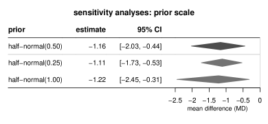
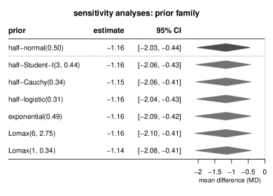
Figure 9: Sensitivity analyses for the MD example (Grande et al.; 2015)¹⁰⁰ from Sec. 5.1 investigating alternative prior distributions for the heterogeneity parameter $\tau$. The left panel shows variations of the scale parameter within the half-normal family, while the right panel corresponds to different prior distribution families with a fixed prior median (here: at 0.34). The “original” result from Sec. 5.1 (half-normal prior with scale 0.5) is shown at the top of each panel.

Parameter estimates for the above analyses (also for heterogeneity $\tau$ and prediction $\theta_{k+1}$) are shown in Table 19. When contrasting results with those obtained based on the noninformative uniform or Jeffreys priors, the estimates differ more substantially. One may argue that, without the use of a weakly informative prior, the empirical data alone are not sufficient to rule out implausible ranges of heterogeneity here. For instance, in case of the improper uniform prior, heterogeneity values beyond $\tau=4.0$ would be considered a-posteriori plausible. This is more than the estimated UISD ($s_{\mathbb{1}}=3.9$), and, looking at Table 4, this would imply variability of $\theta_{i}$ values (differences in mean numbers of symptom days) within ranges of more than $\mu\pm 1\,\mbox{week}$, while the numbers of symptom days themselves were only of the order of one week (see Table 7). Use of a weakly informative prior then allows to rule out such implausible parameter ranges.

Table 19: Estimates and 95% CIs for the heterogeneity ($\tau$), the overall mean effect ($\mu$) and the prediction ($\theta_{k+1}$) corresponding to the discussed sensitivity analyses for the MD example (Grande et al.; 2015)¹⁰⁰. The first line shows the estimates resulting from the half-normal(0.5) prior that was originally proposed in Section 5.1.

	heterogeneity $\tau$		effect $\mu$		prediction $\theta_{k+1}$
prior	median	95% CI	median	95% CI	median	95% CI
half-normal(0.50)	0.29	[0.00, 0.87]	-1.16	[-2.03, -0.44]	-1.15	[-2.50, -0.05]
half-normal(0.25)	0.16	[0.00, 0.47]	-1.11	[-1.73, -0.53]	-1.11	[-1.92, -0.36]
half-normal(1.00)	0.47	[0.00, 1.47]	-1.22	[-2.45, -0.31]	-1.19	[-3.34, 0.48]
half-Student-$t$(3, 0.44)	0.28	[0.00, 0.98]	-1.16	[-2.06, -0.43]	-1.14	[-2.58, 0.00]
half-Cauchy(0.34)	0.23	[0.00, 1.08]	-1.15	[-2.06, -0.41]	-1.13	[-2.61, 0.02]
half-logistic(0.31)	0.29	[0.00, 0.92]	-1.16	[-2.04, -0.43]	-1.15	[-2.55, -0.02]
exponential(0.49)	0.26	[0.00, 1.05]	-1.16	[-2.09, -0.42]	-1.14	[-2.65, 0.04]
Lomax(6, 2.75)	0.25	[0.00, 1.09]	-1.16	[-2.10, -0.41]	-1.14	[-2.67, 0.05]
Lomax(1, 0.34)	0.20	[0.00, 1.16]	-1.14	[-2.08, -0.41]	-1.13	[-2.66, 0.04]
uniform	0.86	[0.00, 4.60]	-1.30	[-3.98, 0.58]	-1.25	[-6.57, 3.13]
Jeffreys	0.62	[0.01, 2.61]	-1.27	[-3.03, -0.05]	-1.24	[-4.55, 1.38]

D.4.3 Log incidence rate ratio example (Anker et al.; 2018)

Regarding the implications of varying the prior scale, the half-normal(1.0) prior was also discussed in Sections 3.4.4 and 4.3 (see especially Table 3 and Figure 3). In the present context, the half-normal(0.25) prior would assign 31% probability to “small” values, 64% and 4.5% to “reasonable” and “fairly high” heterogeneity, respectively, and allow only 0.0063% probability for “fairly extreme” values. The 95% predictive interval (for $\theta_{i}-\mu$) ranges across $\pm 0.55$, corresponding to multiplicative effects of factors of $0.58$ or $1.73$ on the exponentiated scale. With that, the half-normal(0.25) prior confines heterogeneity to a rather optimistic range of values, which would need to be discussed in the exact context of the example. One might need to argue why mostly up to “reasonable” (but virtually no “fairly high” or “fairly extreme”) heterogeneity would be expected; in the present case, such an argument might be made based on the fact that the studies were performed according to similar protocols and executed by the same sponsor.¹¹² Figure 10 (left panel) illustrates the overall effect estimates corresponding to the three prior settings. Although especially the CI width changes slightly, and for the more “optimistic” half-normal(0.25) prior almost excludes zero, the conclusions do not change drastically.

       

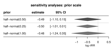
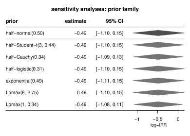
Figure 10: Sensitivity analyses for the IRR example (Anker et al.; 2018)¹¹² from Sec. 5.3.2 investigating alternative prior distributions for the heterogeneity parameter $\tau$. The left panel shows variations of the scale parameter within the half-normal family, while the right panel corresponds to different prior distribution families with a fixed prior median (here: at 0.34). The “original” result from Sec. 5.3.2 (half-normal prior with scale 0.5) is shown at the top of each panel.

Figure 10 (right panel) illustrates the overall effect estimates corresponding to the different prior distribution families. Despite their different appearances and properties (see also Figure 1), the resulting overall effect estimates and CIs again are remarkably similar.

The noninformative priors yield CIs that are wider by factors of roughly 1.5 or 2.1 than for the analysis based on the proposed half-normal(0.5) prior, so the precision gain is quite substantial here. In addition to investigating the priors’ influence on the overall effect ($\mu$), it may also be of interest to consider its effect on prediction intervals, shrinkage estimates, or the heterogeneity’s posterior. Table 20 lists some estimates corresponding to all of the sensitivity analyses discussed above.

Table 20: Estimates and 95% CIs for the heterogeneity ($\tau$), the overall mean effect ($\mu$) and the prediction ($\theta_{k+1}$) corresponding to the discussed sensitivity analyses for the IRR example (Anker et al.; 2018)¹¹². The first line shows the estimates resulting from the half-normal(0.5) prior that was originally proposed in Section 5.3.2.

	heterogeneity $\tau$		effect $\mu$		prediction $\theta_{k+1}$
prior	median	95% CI	median	95% CI	median	95% CI
half-normal(0.50)	0.24	[0.00, 0.75]	-0.49	[-1.10, 0.15]	-0.49	[-1.49, 0.56]
half-normal(0.25)	0.15	[0.00, 0.44]	-0.50	[-1.01, 0.01]	-0.50	[-1.18, 0.20]
half-normal(1.00)	0.34	[0.00, 1.17]	-0.48	[-1.24, 0.35]	-0.49	[-1.89, 1.02]
half-Student-$t$(3, 0.44)	0.23	[0.00, 0.78]	-0.49	[-1.10, 0.15]	-0.49	[-1.49, 0.55]
half-Cauchy(0.34)	0.19	[0.00, 0.77]	-0.49	[-1.09, 0.13]	-0.50	[-1.44, 0.50]
half-logistic(0.31)	0.24	[0.00, 0.77]	-0.49	[-1.10, 0.15]	-0.49	[-1.49, 0.56]
exponential(0.49)	0.21	[0.00, 0.82]	-0.49	[-1.11, 0.15]	-0.49	[-1.50, 0.57]
Lomax(6, 2.75)	0.20	[0.00, 0.82]	-0.49	[-1.10, 0.15]	-0.49	[-1.49, 0.56]
Lomax(1, 0.34)	0.16	[0.00, 0.79]	-0.49	[-1.08, 0.11]	-0.50	[-1.42, 0.48]
uniform	0.46	[0.00, 2.52]	-0.47	[-1.68, 0.91]	-0.48	[-3.05, 2.30]
Jeffreys	0.43	[0.01, 1.61]	-0.47	[-1.39, 0.55]	-0.48	[-2.29, 1.47]

References

- 1 Gelman A, Carlin JB, Stern H, Dunson DB, Vehtari A, Rubin DB. Bayesian data analysis. Boca Raton: Chapman & Hall / CRC. 3rd ed. 2014.
- 2 Gelman A, Hill J. Data analysis using regression and multilevel/hierarchical models. Cambridge University Press . 2007.
- 3 Hedges LV, Olkin I. Statistical methods for meta-analysis. San Diego, CA, USA: Academic Press . 1985.
- 4 Hartung J, Knapp G, Sinha BK. Statistical meta-analysis with applications. Hoboken, NJ, USA: John Wiley & Sons . 2008.
- 5 Jackson D, White IR. When should meta-analysis avoid making hidden normality assumptions?. Biometrical Journal 2018; 60(6): 1040-1058. doi: 10.1002/bimj.201800071
- 6 Röver C, Friede T. Contribution to the discussion of “When should meta-analysis avoid making hidden normality assumptions?”: A Bayesian perspective. Biometrical Journal 2018; 60(6): 1068-1070. doi: 10.1002/bimj.201800179
- 7 Friede T, Röver C, Wandel S, Neuenschwander B. Meta-analysis of few small studies in orphan diseases. Research Synthesis Methods 2017; 8(1): 79-91. doi: 10.1002/jrsm.1217
- 8 Friede T, Röver C, Wandel S, Neuenschwander B. Meta-analysis of two studies in the presence of heterogeneity with applications in rare diseases. Biometrical Journal 2017; 59(4): 658-671. doi: 10.1002/bimj.201500236
- 9 Bender R, Friede T, Koch A, et al. Methods for evidence synthesis in the case of very few studies. Research Synthesis Methods 2018; 9(3): 382-392. doi: 10.1002/jrsm.1297
- 10 Gonnermann A, Framke T, Großhennig A, Koch A. No solution yet for combining two independent studies in the presence of heterogeneity. Statistics in Medicine 2015; 34(16): 2476-2480. doi: 10.1002/sim.6473
- 11 Smith TC, Spiegelhalter DJ, Thomas A. Bayesian approaches to random-effects meta-analysis: A comparative study. Statistics in Medicine 1995; 14(24): 2685-2699. doi: 10.1002/sim.4780142408
- 12 Sutton AJ, Abrams KR. Bayesian methods in meta-analysis and evidence synthesis. Statistical Methods in Medical Research 2001; 10(4): 277-303. doi: 10.1177/096228020101000404
- 13 Schmid CH. Using Bayesian inference to perform meta-analysis. Evaluation & the Health Professions 2001; 24(2): 165-189. doi: 10.1177/01632780122034867
- 14 Spiegelhalter DJ. Incorporating Bayesian ideas into health-care evaluation. Statistical Science 2004; 19(1): 156-174. doi: 10.1214/088342304000000080
- 15 Spiegelhalter DJ, Abrams KR, Myles JP. Bayesian approaches to clinical trials and health-care evaluation. John Wiley & Sons . 2004.
- 16 Higgins JPT, Thompson SG, Spiegelhalter DJ. A re-evaluation of random-effects meta-analysis. Journal of the Royal Statistical Society A 2009; 172(1): 137-159. doi: 10.1111/j.1467-985X.2008.00552.x
- 17 Lunn D, Barrett J, Sweeting A, Thompson S. Fully Bayesian hierarchical modelling in two stages with application to meta-analysis. Journal of the Royal Statistical Society C 2013; 62(4): 551-572. doi: 10.1111/rssc.12007
- 18 Röver C, Friede T. Discrete approximation of a mixture distribution via restricted divergence. Journal of Computational and Graphical Statistics 2017; 26(1): 217-222. doi: 10.1080/10618600.2016.1276840
- 19 Röver C. bayesmeta: Bayesian random-effects meta analysis. R package. URL: http://cran.r-project.org/package=bayesmeta; 2015.
- 20 Röver C. Bayesian random-effects meta-analysis using the bayesmeta R package. Journal of Statistical Software 2020; 93(6): 1-51. doi: 10.18637/jss.v093.i06
- 21 Ding T, Baio G. bmeta: Bayesian meta-analysis and meta-regression. CRAN; 2015. R package.
- 22 Senn S. Trying to be precise about vagueness. Statistics in Medicine 2007; 26(7): 1417-1430. doi: 10.1002/sim.2639
- 23 van Dongen S. Prior specification in Bayesian statistics: Three cautionary tales. Journal of Theoretical Biology 2006; 242(1): 90-100. doi: 10.1016/j.jtbi.2006.02.002
- 24 Williams DR, Rast P, Bürkner PC. Bayesian meta-analysis with weakly informative prior distributions. PsyArXiv 2018. doi: 10.17605/OSF.IO/7TBRM
- 25 Gelman A. Prior distributions for variance parameters in hierarchical models. Bayesian Analysis 2006; 1(3): 515-534. doi: 10.1214/06-BA117A
- 26 Neuenschwander B, Schmidli H. Use of historical data. In: Lesaffre E, Baio G, Boulanger B. , eds. Bayesian Methods in Pharmaceutical ResearchChapmann & Hall / CRC. 2020 (pp. 111-137)
- 27 Prevost TC, Abrams KR, Jones DR. Hierarchical models in generalized synthesis of evidence: an example based on studies of breast cancer screening. Statistics in Medicine 2000; 19(24): 3359-3376. doi: 10.1002/1097-0258(20001230)19:24<3359::AID-SIM710>3.0.CO;2-N
- 28 Dias S, Sutton AJ, Welton NJ, Ades AE. Evidence synthesis for decision making 3: Heterogeneity—subgroups, meta-regression, bias, and bias-adjustment. Medical Decision Making 2013; 33(5): 618-640. doi: 10.1177/0272989X13485157
- 29 Debray TPA, Moons KGM, Valkenhoef vG, et al. Get real in individual participant data (IPD) meta-analysis: a review of the methodology. Research Synthesis Methods 2015; 6(4): 293-309. doi: 10.1002/jrsm.1160
- 30 Stewart L, Moher D, Shekelle P. Why prospective registration of systematic reviews makes sense. Systematic Reviews 2012; 1: 7. doi: 10.1186/2046-4053-1-7
- 31 Stevens JW. A note on dealing with missing standard errors in meta-analyses of continuous outcome measures in WinBUGS. Pharmaceutical Statistics 2011; 10(4): 374-378. doi: 10.1002/pst.491
- 32 Borenstein M, Hedges LV, Higgins JPT, Rothstein HR. A basic introduction to fixed-effect and random-effects models for meta-analysis. Research Synthesis Methods 2010; 1(2): 97-111. doi: 10.1002/jrsm.12
- 33 Wandel S, Neuenschwander B, Röver C, Friede T. Using phase II data for the analysis of phase III studies: an application in rare diseases. Clinical Trials 2017; 14(3): 277-285. doi: 10.1177/1740774517699409
- 34 Pullenayegum EM. An informed reference prior for between-study heterogeneity in meta-analyses of binary outcomes. Statistics in Medicine 2011; 30(26): 3082-3094. doi: 10.1002/sim.4326
- 35 Jaynes ET. Probability theory: The logic of science. Cambridge: Cambridge University Press . 2003.
- 36 Gelman A. Bayes, Jeffreys, prior distributions and the philisophy of statistics. Statistical Science 2009; 24(2): 176-178.
- 37 Cole SR, Chu H, Greenland S. Maximum likelihood, profile likelihood, and penalized likelihood: A primer. American Journal of Epidemiology 2014; 179(2): 252-260. doi: 10.1093/aje/kwt245
- 38 Chung Y, Rabe-Hesketh S, Choi IH. Avoiding zero between-study variance estimates in random-effects meta-analysis. Statistics in Medicine 2013; 32(23): 4071-4089. doi: 10.1002/sim.5821
- 39 Klein N, Kneib T. Scale-dependent priors for variance parameters in structured additive distributional regression. Bayesian Analysis 2016; 11(4): 1071-1106. doi: 10.1214/15-BA983
- 40 Bayarri MJ, Berger JO. The interplay of Bayesian and frequentist analysis. Statistical Science 2004; 19(1): 58-80. doi: 10.1214/088342304000000116
- 41 Kass RE. Statistical inference: the big picture. Statistical Science 2011; 26(1): 1-9. doi: 10.1214/10-STS337
- 42 Spiegelhalter DJ, Freedman L. Bayesian approaches to randomized trials. Journal of the Royal Statistical Society A 1994; 157(3): 357-416. doi: 10.2307/2983527
- 43 Jaynes ET. Confidence intervals vs. Bayesian intervals. In: Harper WL, Hooker CA. , eds. Foundations of probability theory, statistical inference, and statistical theories of scienceDordrecht: D. Reidel. 1976 (pp. 175-257)
- 44 Datta GS, Sweeting TJ. Probability matching priors. In: Dey DK, Rao CR. , eds. Handbook of Statistics. 25. Elsevier B. V. 2005 (pp. 91-114)
- 45 Dawid AP. The well-calibrated Bayesian. Journal of the American Statistical Association 1982; 77(379): 605-610. doi: 10.1080/01621459.1982.10477856
- 46 Mandelkern M. Setting confidence intervals for bounded parameters (with discussion). Statistical Science 2002; 17(2): 149-172. doi: 10.1214/ss/1030550859
- 47 Gneiting T, Balabdaoui F, Raftery AE. Probabilistic forecasts, calibration and sharpness. Journal of the Royal Statistical Society B 2007; 69(2): 243-268. doi: 10.1111/j.1467-9868.2007.00587.x
- 48 Gelman A. Prior choice recommendations. online; 2018. URL: https://github.com/stan-dev/stan/wiki/Prior-Choice-Recommendations#prior-for-scale-parameters-in-hierarchical-models.
- 49 O’Hagan A, Pericchi L. Bayesian heavy-tailed models and conflict resolution: A review. Brazilian Journal of Probability and Statistics 2012; 26(4): 372-401. doi: 10.1214/11-BJPS164
- 50 Jaynes ET. Prior probabilities. IEEE Transactions on Systems Science and Cybernetics 1968; SEC-4(3): 227-241. doi: 10.1109/TSSC.1968.300117
- 51 Morita S, Thall P, Müller P. Determining the effective sample size of a parametric prior. Biometrics 2008; 64(2): 595-602. doi: 10.1111/j.1541-0420.2007.00888.x
- 52 Neuenschwander B, Weber S, Schmidli H, O’Hagan A. Predictively consistent prior effective sample sizes. Biometrics 2020; 76(2): 578-587. doi: 10.1111/biom.13252
- 53 Evans M, Jang GH. Weak informativity and the information in one prior relative to another. Statistical Science 2011; 26(3): 423-439. doi: 10.1214/11-STS357
- 54 Kass RE, Wasserman L. A reference Bayesian test for nested hypotheses and its relationship to the Schwarz criterion. Journal of the American Statistical Association 1995; 90(431): 928-934. doi: 10.2307/2291327
- 55 Lazar N. Ockham’s razor. Wiley Interdisciplinary Reviews: Computational Statistics 2010; 12(1): 243-246. doi: 10.1002/wics.75
- 56 Ren S, Oakley JE, Stevens JW. Incorporating genuine prior information about between-study heterogeneity in random effects pairwise and network meta-analyses. Medical Decision Making 2018; 38(4): 531-542. doi: 10.1177/0272989X18759488
- 57 Hampson LV, Whitehead J, Eleftheriou D, Brogan P. Bayesian methods for the design and interpretation of clinical trials in very rare diseases. Statistics in Medicine 2014; 33(24): 4186-4201. doi: 10.1002/sim.6225
- 58 Polson NG, Scott JG. On the half-Cauchy prior for a global scale parameter. Bayesian Analysis 2012; 7(4): 887-902. doi: 10.1214/12-BA730
- 59 Cunanan KM, Iasonos A, Shen R, Gönen M. Variance prior specification for a basket trial design using Bayesian hierarchical modeling. Clinical Trials 2018. doi: 10.1177/1740774518812779
- 60 Schmid CH, Carlin BP, Welton NJ. Bayesian methods for meta-analysis. In: Schmid CH, White I, Stijnen T. , eds. Handbook of meta-analysisNew York: Chapman and Hall/CRC. 2021.
- 61 Ades AE, Lu G, Higgins JPT. The interpretation of random-effects meta-analysis in decision models. Medical Decision Making 2005; 25(6): 646-654. doi: 10.1177/0272989X05282643
- 62 Röver C, Friede T. Dynamically borrowing strength from another study. Statistical Methods in Medical Research 2020; 29(1): 293-308. doi: 10.1177/0962280219833079
- 63 Röver C, Friede T. Bounds for the weight of external data in shrinkage estimation. arXiv preprint 2004.02525 2020.
- 64 Shaked M, Shanthikumar JG. Stochastic orders. New York: Springer-Verlag . 2007.
- 65 Mood AM, Graybill FA, Boes DC. Introduction to the theory of statistics. New York: McGraw-Hill. 3rd ed. 1974.
- 66 Mȩczarski M. Stochastic orders in the Bayesian framework. Collegium of Economic Analysis Annals 37, Instytut Ekonometrii, Szkoła Główna Handlowa w Warszawie (Institute of Econometrics, Warsaw School of Economics); Warsaw: 2015.
- 67 Bartoszewicz J, Skolimowska M. Preservation of classes of life distributions and stochastic orders under weighting. Statistics & Probability Letters 2006; 76(6): 587-596. doi: 10.1016/j.spl.2005.09.003
- 68 Berger J, Berliner LM. Robust Bayes and empirical Bayes analysis with -contaminated priors. The Annals of Statistics 1986; 14(2): 461-486. doi: 10.1214/aos/1176349933
- 69 Berger JO. Statistical decision theory and Bayesian analysis. Springer-Verlag. 2nd ed. 1985.
- 70 DuMouchel W. Predictive cross-validation of Bayesian meta-analyses. In: Bernardo JM, Berger JO, Dawid AP, Smith AFM. , eds. Bayesian Statistics 5Oxford University Press. 1996 (pp. 107-127).
- 71 DuMouchel WH, Normand SL. Computer modeling strategies for meta-analysis. In: Stangl DK, Berry DA. , eds. Meta-analysis in medicine and health policyCRC Press. 2000 (pp. 127-178).
- 72 Schmidli H, Gsteiger S, Roychoudhury S, O’Hagan A, Spiegelhalter D, Neuenschwander B. Robust meta-analytic-predictive priors in clinical trials with historical control information. Biometrics 2014; 70(4): 1023-1032. doi: 10.1111/biom.12242
- 73 Röver C, Wandel S, Friede T. Model averaging for robust extrapolation in evidence synthesis. Statistics in Medicine 2018; 38(4): 674-694. doi: 10.1002/sim.7991
- 74 Rhodes KM, Turner RM, Higgins JPT. Predictive distributions were developed for the extent of heterogeneity in meta-analyses of continuous outcome data. Journal of Clinical Epidemiology 2015; 68(1): 52-60. doi: 10.1016/j.jclinepi.2014.08.012
- 75 Turner RM, Jackson D, Wei Y, Thompson SG, Higgins PT. Predictive distributions for between-study heterogeneity and simple methods for their application in Bayesian meta-analysis. Statistics in Medicine 2015; 34(6): 984-998. doi: 10.1002/sim.6381
- 76 Rücker G, Schwarzer G, Carpenter J, Okin I. Why add anything to nothing? The arcsine difference as a measure of treatment effect in meta-analysis with zero cells. Statistics in Medicine 2009; 28(5): 721-738. doi: 10.1002/sim.3511
- 77 Neuenschwander B, Capkun-Niggli G, Branson M, Spiegelhalter DJ. Summarizing historical information on controls in clinical trials. Clinical Trials 2010; 7(1): 5-18. doi: 10.1177/1740774509356002
- 78 Higgins JPT, Whitehead A. Borrowing strength from external trials in a meta-analysis. Statistics in Medicine 1996; 15(24): 2733-2749. doi: 10.1002/(SICI)1097-0258(19961230)15:24<2733::AID-SIM562>3.0.CO;2-0
- 79 Turner RM, Davey J, Clarke MJ, Thompson SG, Higgins JPT. Predicting the extent of heterogeneity in meta-analysis, using empirical data from the Cochrane Database of Systematic Reviews. International Journal of Epidemiology 2012; 41(3): 818-827. doi: 10.1093/ije/dys041
- 80 Kontopantelis E, Springate DA, Reeves D. A re-analysis of the Cochrane Library data: The dangers of unobserved heterogeneity in meta-analyses. PLoS ONE 2013; 8(7): e69930. doi: 10.1371/journal.pone.0069930
- 81 Steel P, Kammeyer-Mueller J, Paterson TA. Improving the meta-analytic assessment of effect size variance with an informed Bayesian prior. Journal of Management 2015; 41(2): 718-743. doi: 10.1177/0149206314551964
- 82 van Erp S, Verhagen J, Grasman RPPP, Wagenmakers EJ. Estimates of between-study heterogeneity for 705 meta-analyses reported in Psychological Bulletin from 1990–2013. Journal of Open Psychology Data 2017; 5(4). doi: 10.5334/jopd.33
- 83 Seide SE, Röver C, Friede T. Meta-analysis data extracted from IQWiG publications. Göttingen Research Online; 2018. doi: 10.25625/BWYBNK.
- 84 Seide SE, Röver C, Friede T. Likelihood-based random-effects meta-analysis with few studies: Empirical and simulation studies. BMC Medical Research Methodology 2019; 19: 16. doi: 10.1186/s12874-018-0618-3
- 85 Günhan BK, Röver C, Friede T. Random-effects meta-analysis of few studies involving rare events. Research Synthesis Methods 2020; 11(1): 74-90. doi: 10.1002/jrsm.1370
- 86 Hsu H, Lachenbruch PA. Paired test. In: Armitage P, Colton T. , eds. Encyclopedia of BiostatisticsWiley & Sons. 2nd ed. 2005
- 87 Baker RD, Jackson D. Meta-analysis inside and outside particle physics: two traditions that should converge?. Research Synthesis Methods 2013; 4(2): 109-124. doi: 10.1002/jrsm.1065
- 88 Menard S. Standardized regression coefficients. In: Lewis-Beck MS, Bryman A, Liao TF. , eds. The Sage Encyclopedia of Social Science Research MethodsThousand Oaks, CA, USA: Sage Publications. 2004 (pp. 1069-1070)
- 89 Cohen J. Statistical power analysis for the behavioural sciences. New York: Routledge. 2nd ed. 1988
- 90 Sawilowsky SS. New effect size rules of thumb. Journal of Modern Applied Statistical Methods 2009; 8(2): 597-599. doi: 10.22237/jmasm/1257035100
- 91 Viechtbauer W. Conducting meta-analyses in R with the metafor package. Journal of Statistical Software 2010; 36(3). doi: 10.18637/jss.v036.i03
- 92 Trikalinos TA, Trow P, Schmid CH. Simulation-based comparison of methods for meta-analysis of proportions and rates. AHRQ Publication 13(14)-EHC084-EF, Agency for Healthcare Research and Quality; Rockville, MD, USA: 2013.
- 93 Becker B, Wu MJ. The synthesis of regression slopes in meta-analysis. Statistical Science 2007; 22(3): 414-429. doi: 10.1214/07-STS243
- 94 Gelman A, Jakulin A, Pittau MG, Su YS. A weakly informative default prior distribution for logistic and other regression models. The Annals of Applied Statistics 2008; 2(4): 1360-1383. doi: 10.1214/08-AOAS191
- 95 Newman TB, Browner WS. In defense of standardized regression coefficients. Epidemiology 1991; 2(5): 383-386. doi: 10.1097/00001648-199109000-00014
- 96 Greenland S, Maclure M, Schlesselman JJ, Poole C, Morgenstern H. Standardized regression coefficients: A further critique and review of some alternatives. Epidemiology 1991; 2(5): 387-392. doi: 10.1097/00001648-199109000-00016
- 97 Bring J. How to standardize regression coefficients. The American Statistician 1994; 48(3): 209-213.
- 98 Schulze R. Meta-analysis: a comparison of approaches. Göttingen: Hogrefe & Huber . 2004.
- 99 Armitage P. Correlation. In: Armitage P, Colton T. , eds. Encyclopedia of BiostatisticsWiley & Sons. 2nd ed. 2005
- 100 Grande AJ, Keogh J, Hoffmann TC, Beller EM, Del Mar CB. Exercise versus no exercise for the occurrence, severity and duration of acute respiratory infections. Cochrane Database of Systematic Reviews 2015; 6: CD010596. doi: 10.1002/14651858.CD010596.pub2
- 101 Del Mar C. Understanding the burden of acute respiratory infections. Annales Nestlé 2000; 58(2): 41-48.
- 102 Ambrosino N, others . Acute lower respiratory infections. In: Gibson GJ, Loddenkemper R, Sibille Y, Lundbäck B. , eds. European Lung White BookEuropean Respiratory Society (ERS). 2013 (pp. 210-223).
- 103 Sanders S, Doust J, Del Mar C. Acute respiratory infections. Health Sciences & Medicine papers 86, Bond University; Robina, QLD, Australia: 2008.
- 104 Aalbers S, Fusar-Poli L, Freeman RE, et al. Music therapy for depression. Cochrane Database of Systematic Reviews 2017; 11: CD004517. doi: 10.1002/14651858.CD004517.pub3
- 105 Albornoz Y. The effects of group improvisational music therapy on depression in adolescents and adults with substance abuse: a randomized controlled trial. Nordic Journal of Music Therapy 2011; 20(3). doi: 10.1080/08098131.2010.522717
- 106 Hamilton M. A rating scale for depression. Journal of Neurology, Neurosurgery & Psychiatry 1960; 23: 56-62. doi: 10.1136/jnnp.23.1.56
- 107 Kriston L, von Wolff A. Not as golden as standards should be: Interpretation of the Hamilton rating scale for depression. Journal of Affective Disorders 2011; 128(1): 175-177. doi: 10.1016/j.jad.2010.07.011
- 108 Furukawa T, Akechi T, Azuma H, Okuyama T, Higuchi T. Evidence-based guidelines for interpretation of the Hamilton rating scale for depression. Journal of Clinical Psychopharmacology 2007; 27(5): 531-534. doi: 10.1097/JCP.0b013e31814f30b1
- 109 Masson SC, Tejani AM. Minimum clinically important differences identified for commonly used depression rating scales. Journal of Clinical Epidemiology 2013; 66(7). doi: 10.1016/j.jclinepi.2013.01.010
- 110 Crins ND, Röver C, Goralczyk AD, Friede T. Interleukin-2 receptor antagonists for pediatric liver transplant recipients: A systematic review and meta-analysis of controlled studies. Pediatric Transplantation 2014; 18(8): 839-850. doi: 10.1111/petr.12362
- 111 Goralczyk AD, Hauke N, Bari N, Tsui TY, Lorf T, others . Interleukin-2 receptor antagonists for liver transplant recipients: A systematic review and meta-analysis of controlled studies. Hepatology 2011; 54(2): 541-554. doi: 10.1002/hep.24385
- 112 Anker SD, Kirwan BA, van Veldhuisen DJ, others . Effects of ferric carboxymaltose on hospitalisations and mortality rates in iron-deficient heart failure patients: an individual patient data meta-analysis. European Journal of Heart Failure 2018; 20(1): 125-133. doi: 10.1002/ejhf.823
- 113 Dias S, Ades AE. Absolute or relative effects? Arm-based synthesis of trial data. Research Synthesis Methods 2016; 7(1): 23-28. doi: 10.1002/jrsm.1184
- 114 White I, Turner RM, Karahalios A, Salanti G. A comparison of arm-based and contrast-based models for network meta-analysis. Statistics in Medicine 2019; 38(27): 5197-5213. doi: 10.1002/sim.8360
- 115 Feagan BG, others . Treatment of ulcerative colitis with a humanized antibody to the integrin. The New England Journal of Medicine 2005; 352(24): 2499-2507. doi: 10.1056/NEJMoa042982
- 116 Bergau L, Tichelbäcker T, Kessel B, et al. Predictors of mortality and ICD shock therapy in primary prophylactic ICD patients - a systematic review and meta-analysis. PLoS ONE 2016; 12(10): e0186387. doi: 10.1371/journal.pone.0186387
- 117 Lang RM, Badano LP, Mor-Avi V, Afilalo J, others . Recommendations for cardiac chamber quantification by echocardiography in adults: an update from the American Society for Echocardiography and the European Association for Cardiovascular Imaging. European Heart Journal - Cardiovascular Imaging 2015; 16(3): 233-271. doi: 10.1093/ehjci/jev014
- 118 Tracy CM, Epstein AE, Darbar D, others . 2012 ACCF/AHA/HRS focused update incorporated into the ACCF/AHA/HRS 2008 guidelines for device-based therapy of cardiac rhythm abnormalities: A report of the American College of Cardiology Foundation / American Heart Association task force on practice guidelines and the Heart Rhythm Society. Journal of the American College of Cardiology 2013; 61(3): e6-e75. doi: 10.1016/j.jacc.2012.11.007
- 119 Molloy GJ, O’Carroll RE, Ferguson E. Conscientiousness and medication adherence: A meta-analysis. Annals of Behavioural Medicine 2014; 47(1): 92-101. doi: 10.1007/s12160-013-9524-4
- 120 Lindley DV. A statistical paradox. Biometrika 1957; 44(1/2): 187-192. doi: 10.1093/biomet/44.1-2.187
- 121 Deeks JJ, Altman D. Effect measures for meta-analysis of trials with binary outcomes. In: Egger M, Davey Smith G, Altman D. , eds. Systematic reviews in health care: Meta-analysis in contextLondon: BMJ Publishing. 2nd ed. 2001 (pp. 313-335)
- 122 Rothstein HR, Sutton AJ, Borenstein M. , eds.Publication bias in meta-analysis. Wiley & Sons . 2005.
- 123 Williamson PR, Gamble C, Altman DG, Hutton JL. Outcome selection bias in meta-analysis. Statistical Methods in Medical Research 2005; 14(5): 515-524.
- 124 Wang Z, Lin L, Hodges JS, Chu H. The impact of covariance priors on arm-based Bayesian network meta-analyses with binary outcomes. Statistics in Medicine 2020. doi: 10.1002/sim.8580
- 125 Debray T, Moons KGM, Abo-Zaid GMA, Koffijberg H, Riley RD. Individual participant data meta-analysis for a binary outcome: one-stage or two-stage?. PLoS ONE 2013; 8(4): e60650. doi: 10.1371/journal.pone.0060650
- 126 Burke DL, Ensor J, Riley RD. Meta-analysis using individual participant data: one-stage and two-stage approaches, and why they may differ. Statistics in Medicine 2017; 36(5): 855-875. doi: 10.1002/sim.7141
- 127 Kontopantelis E. A comparison of one-stage vs two-stage individual patient data meta-analysis methods: a simulation study. Research Synthesis Methods 2018; 9(3): 417-430. doi: 10.1002/jrsm.1303
- 128 Brown H, Prescott R. Applied mixed models in medicine. John Wiley & Sons. 3rd ed. 2014.
- 129 Higgins JPT, Thomas J, Chandler J, et al. , eds.Cochrane handbook for systematic reviews of interventions. Hoboken, NJ, USA: Wiley & Sons. 2nd ed. 2019
- 130 Johnson NL, Kotz S, Balakrishnan N. Continuous univariate distributions. New York: John Wiley & Sons. 2nd ed. 1994.
- 131 Psarakis S, Panaretos J. The folded distribution. Communications in Statistics — Theory and Methods 1990; 19(7): 2717-2734.
- 132 Lindsay BG. Mixture models: theory, geometry and applications. 5 of NSF-CBMS Regional Conference Series in Probability and Statistics. Hayward, CA, USA: Institute of Mathematical Statistics . 1995.
- 133 Bernardo JM, Smith AFM. Bayesian theory. Chichester, UK: Wiley . 1994.
- 134 Jackson D, Law M, Stijnen T, Viechtbauer W, White IR. A comparison of seven random-effects models for meta-analyses that estimate the summary odds ratio. Statistics in Medicine 2018; 37(7): 1059-1085. doi: 10.1002/sim.7588