Experimental quantification of the entanglement of noisy twin beams

Abstract

Gradual loss of the entanglement of a twin beam containing around 25 photon pairs with the increasing external noise is experimentally investigated. The entanglement is quantified by the non-classicality depths and the non-classicality counting parameters related to several non-classicality criteria. The reduction of intensity moments of the analyzed multi-mode twin beams to single-mode ones allows to determine the negativity as another quantifier of the entanglement. Both the raw photocount histograms and the reconstructed photon-number distributions are analyzed in parallel.

I Introduction

Twin beams (TWBs) ideally composed of photon pairs have very interesting quantum properties: They exhibit the entanglement between the photons belonging to the same photon pair that occurs in different degrees of freedom including frequencies, polarizations or propagation directions. At the same time, however, the TWBs containing on average typically more than one photon pair exhibit perfect correlations between the numbers of the signal and idler photons, that represent another attribute of the TWB quantumness. The entanglement in the TWB, as the TWB prominent feature, finds its applications in metrology (measurement of ultra-short time intervals, absolute detector calibration Migdall (1999); Peřina Jr. et al. (2012a)), quantum communications (reduction of noise, quantum cryptography) and various quantum-information protocols Nielsen and Juang (2000). Quantum states with specific properties may be obtained using various types of post-selection realized on the TWB Magańa-Loaiza et al. (2019). However, the noise superimposed on the TWB occurs in a smaller or greater amount in all these applications. For example, in the quantum-communication applications the noise increases linearly with the distance Allevi and Bondani (2018). As certain minimal amount of the entanglement is indispensable for all applications of TWBs, restriction to the maximal tolerable amount of the noise occurs. This brings the need to quantify the TWB entanglement and its relationship to the noise. The noise may originate either in the sources outside the TWB or in photon pairs of the TWB being partly absorbed during their propagation (typically in optical fibers). In this contribution, we suggest three theoretical concepts how to quantify the TWB entanglement. We verify these concepts experimentally: We generate a TWB with around 25 photon pairs on average and superimpose an additional noise with the increasing intensity onto both signal and idler beams.

Quantification of the entanglement of TWBs is not an easy task because the TWBs are typically (spectrally and spatially) multi-mode and as such they are properly characterized by quasi-distributions of the overall signal and idler (integrated) intensities, instead of amplitudes. This comes from the fact that the multi-mode character of the fields makes the information about the phases of individual spatio-spectral modes as well as their individual intensities unimportant. A larger number of modes prevents the application of the homodyne tomography Leonhardt (1997); Lvovsky and Raymer (2009) in the experimental investigations of TWBs, as well as the use of the entanglement witnesses based on the moments of fields’ amplitudes Duan et al. (2000); Simon (2000); Shchukin et al. (2005); Miranowicz et al. (2010). Quantification of the entanglement of multi-mode optical fields represents a serious and demanding problem even in specific cases when individual modes and their inter-modal correlations are measured Gerke et al. (2015); Harder et al. (2016). In the case of multi-mode TWBs, we do not have access to the properties of individual modes. However, we know that the reduced states of the signal and idler beams are multi-mode thermal Mandel and Wolf (1995), i.e. they are purely classical, as a consequence of the spontaneous emission of photon pairs in the process of spontaneous parametric down-conversion Boyd (2003). This means that the quantification of TWB entanglement can be mapped onto the quantification of the TWB non-classicality.

In general, the non-classicality of a state is recognized by the negative values of quasi-distributions of intensities (even being in the form of generalized functions) Glauber (1963); Peřina (1991). In the case of multi-mode TWBs, the problem of non-classicality identification can be considerably simplified when applying suitable non-classicality identifiers/witnesses (NI) Peřina Jr. et al. (2017); Arkhipov and Peřina Jr (2018); Arkhipov et al. (2016) that are conveniently based on the intensity moments. The fields’ intensities and their moments can be measured by photon-number-resolving detectors that provide the corresponding photocount distributions Haderka et al. (2005); Allevi et al. (2012); Peřina Jr. et al. (2013); Harder et al. (2016); Chesi et al. (2019); Magańa-Loaiza et al. (2019). We note that also the NIs based directly on the elements of photocount (or photon-number) distributions may also be used for this purpose Klyshko (1996); Waks et al. (2006); Wakui et al. (2014); Peřina Jr. et al. (2017). The quantification of non-classicality/entanglement is then reached by applying the concept of the Lee non-classicality depth Lee (1991) or the approach leading to the non-classicality counting parameter Peřina Jr. et al. (2019).

Here, we suggest and verify an alternative approach in which we first determine the intensity moments appropriate to one typical (paired) mode and then we use these intensity moments in the formula for the negativity of a Gaussian two-mode field Adesso and Illuminati (2007); Arkhipov et al. (2015) to directly quantify the TWB entanglement. The negativity Hill and Wootters (1997) exploits the properties of the partially-transposed statistical operator Peres (1996); Horodecki et al. (1996) to quantify the amount of the entanglement in a composed quantum system.

The paper is organized as follows. Non-classicality and entanglement identifiers and quantifiers are theoretically introduced in Sec. II. The experimental setup, performed experiment and the reconstruction method for revealing a TWB joint photon-number distribution from the experimental photocount histogram are described in Sec. III. Degradation of the non-classicality and entanglement caused by an additional noise with the increasing intensity is discussed in Sec. IV using the theoretical tools of Sec. II. Sec. V brings conclusions.

II Non-classicality and entanglement identification and quantification

For TWBs, the noise-reduction-factor $R$ is the commonly determined quantity that may also indicate their non-classicality:

$$R=1+\frac{\langle\left[\Delta(W_{\rm s}-W_{\rm i})\right]^{2}\rangle}{\langle{W_{\rm s}}\rangle+\langle{W_{\rm i}}\rangle},$$ (1)

where $W_{\rm s}$ ($W_{\rm i}$) denotes the signal- (idler-) field (integrated) intensity and $\Delta W=W-\langle W\rangle$. According to its definition the noise-reduction-factor $R$ quantifies pairing of the photons in a TWB. For an ideal TWB composed of only photon pairs, it equals to zero. If an additional noise on the top of the paired photons is present in the TWB, $R>0$. The larger the amount of the noise, the greater the value of $R$. It can be shown that the TWBs with $R<1$ are nonclassical.

The intensity moments Mandel and Wolf (1995); Peřina (1991) needed for the determination of the noise-reduction-factor $R$ as well as other characteristics of the TWBs are commonly derived from the moments of the reconstructed photon-number distribution $p(n_{\rm s},n_{\rm i})$. This distribution is obtained by the reconstruction from the experimental photocount histogram $f(c_{\rm s},c_{\rm i})$. The intensity moments $\langle W_{\rm s}^{k}W_{\rm i}^{l}\rangle$ represent the normally-ordered photon-number moments. They are derived from the usual photon-number moments $\langle n_{\rm s}^{i}n_{\rm i}^{j}\rangle$ using the following linear relations valid for one effective bosonic mode with the operators fulfilling the canonical commutation relations ($k,l=1,2,\ldots$) Saleh (1978); Mandel and Wolf (1995); Peřina (1991):

$$\langle W_{\rm s}^{k}W_{\rm i}^{l}\rangle=\sum_{m=0}^{k}S(k,m)\sum_{j=0}^{l}S(l,j)\langle n_{\rm s}^{m}n_{\rm i}^{j}\rangle.$$ (2)

In Eq. (2), symbol $S$ stands for the Stirling numbers of the first kind Gradshtein and Ryzhik (2000).

The reconstruction of a photon-number distribution removes the ’distortions’ in the experimental photocount histogram caused by the detector. As such it improves in general the characteristics of the analyzed field, especially its non-classicality. To assess the parameters/quality of the directly measured photocount histogram, we may assume that it was obtained by an ideal detector whose operation does not require any correction. In this case, we may consider in the r.h.s. of Eq. (2) the photoucount moments $\langle c_{\rm s}^{i}c_{\rm i}^{j}\rangle$ instead of the photon-number moments $\langle n_{\rm s}^{i}n_{\rm i}^{j}\rangle$ and determine the corresponding intensity moments. Such intensity moments derived from the photocount moments can then be used in parallel to the usual intensity moments of Eq. (2) to determine the quantities of interest and discuss the related properties. We note that we systematically use the quantities $c_{\rm s}$ and $c_{\rm i}$ to count the numbers of detected electrons (photocounts) whereas the numbers $n_{\rm s}$ and $n_{\rm i}$ quantify photon numbers in the reconstructed TWB.

The real experimental quantification of the TWB non-classicality can be based upon suitable NIs for which the non-classicality depths $\tau$ introduced in Lee (1991) or the non-classicality counting parameters $\nu$ defined in Peřina Jr. et al. (2019) are determined (for details, see below). Following the comprehensive analysis of NIs based on the intensity moments of TWBs Peřina Jr. et al. (2017), we consider the following three representative NIs:

$$M \equiv \langle W_{\rm s}^{2}\rangle\langle W_{\rm i}^{2}\rangle-\langle W_{\rm s}W_{\rm i}\rangle^{2}<0,$$

$$E_{2} \equiv \langle W_{\rm s}^{2}\rangle+\langle W_{\rm i}^{2}\rangle-2\langle W_{\rm s}W_{\rm i}\rangle<0,$$

$$E_{3} \equiv \langle W_{\rm s}^{3}\rangle+\langle W_{\rm i}^{3}\rangle-\langle W_{\rm s}^{2}W_{\rm i}\rangle-\langle W_{\rm s}W_{\rm i}^{2}\rangle<0.$$ (3)

The NI $M$ has a privileged position among other NIs based on the intensity moments as it only identifies the non-classicality in an arbitrary single-mode TWB Arkhipov and Peřina Jr (2018). Whereas the NI $M$ contains the intensity moments in the cumulative fourth order, the other considered NI $E_{2}$ uses just the second-order intensity moments. For this reason, the most commonly applied NI $E_{2}$ is determined with better experimental precision than the NI $M$. We note that for a balanced TWB with $\langle W_{\rm s}\rangle=\langle W_{\rm i}\rangle$, $E_{2}<0$ is equivalent to $R<1$. In general, the condition $R<1$ can be transformed into the inequality

$$E_{2}+\left(\langle W_{\rm s}\rangle-\langle W_{\rm i}\rangle\right)^{2}<0$$ (4)

and so the NI $E_{2}$ is stronger in identifying the non-classicality than the noise-reduction-factor $R$. On the other hand, the last considered NI $E_{3}$ directly involves the third-order intensity moments and as such it monitors the higher (third) -order non-classicality.

The performance of the above NIs can directly be compared for single-mode fields. In this case, a TWB is nonclassical provided that $Q\equiv 2\langle W_{\rm s}\rangle\langle W_{\rm i}\rangle-\langle W_{\rm s}W_{\rm i}\rangle<0$ Peřina and Křepelka (2011). Using the formulas $\langle W_{a}^{2}\rangle=2\langle W_{a}\rangle^{2}$, $\langle W_{a}^{3}\rangle=6\langle W_{a}\rangle^{3}$, $a={\rm s,i}$, $\langle W_{\rm s}^{2}W_{\rm i}\rangle=2\langle W_{\rm s}W_{\rm i}\rangle\langle W_{\rm s}\rangle$, and $\langle W_{\rm s}W_{\rm i}^{2}\rangle=2\langle W_{\rm s}W_{\rm i}\rangle\langle W_{\rm i}\rangle$ valid for the single-mode Gaussian fields, we rewrite Eqs. (3) in the form:

$$M = Q(2\langle W_{\rm s}\rangle\langle W_{\rm i}\rangle+\langle W_{\rm s}W_{\rm i}\rangle)<0,$$

$$E_{2} = 2Q+2(\langle W_{\rm s}\rangle-\langle W_{\rm i}\rangle)^{2}<0,$$

$$E_{3} = 2Q(\langle W_{\rm s}\rangle+\langle W_{\rm i}\rangle)+2(\langle W_{\rm s}\rangle^{3}+\langle W_{\rm i}\rangle^{3})$$ (5)

$$\mbox{}+4(\langle W_{\rm s}\rangle-\langle W_{\rm i}\rangle)^{2}(\langle W_{\rm s}\rangle+\langle W_{\rm i}\rangle)<0.$$

According to Eqs. (5), the NI $M$ identifies all nonclassical single-mode TWBs, whereas the NIs $E_{2}$ and $E_{3}$ are weaker than the condition $Q<0$. We note that nonclassical balanced TWBs are also completely identified by the NI $E_{2}$.

The concept of the non-classicality depth (ND) $\tau$ Lee (1991) is based upon the behavior of quasi-distributions in the phase space of an optical field in relation to different field-operator orderings. It uses the fact that the amount of non-classicality decreases as we move from the normal ordering, that corresponds to the usual detection by quadratic intensity detectors, to the anti-normal ordering, in which any optical field exhibits only the classical properties. The ND $\tau$ gives the distance on the ordering-parameter axis $s$ between the point at which the non-classicality is lost $s_{\rm th}$ and the point of the normal ordering $s=1$:

$$\tau=(1-s_{\rm th})/2.$$ (6)

The threshold ordering parameter $s_{\rm th}$ is determined so that the corresponding $s$-ordered intensity moments $\langle W_{\rm s}^{k}W_{\rm i}^{l}\rangle_{s}$ nullify the corresponding NI. The $s$-ordered intensity moments are given as Peřina (1991):

$$\langle W_{\rm s}^{k}W_{\rm i}^{l}\rangle_{s}=\left(\frac{2}{1-s}\right)^{k+l}\left\langle{\rm L}_{k}\left(\frac{2W_{\rm s}}{s-1}\right){\rm L}_{l}\left(\frac{2W_{\rm i}}{s-1}\right)\right\rangle$$ (7)

and ${\rm L}_{k}$ denotes the $k$-th Laguerre polynomial Gradshtein and Ryzhik (2000). Whereas we have $0\leq\tau\leq 1$ for an arbitrary field, the value of ND $\tau$ of any nonclassical Gaussian beam cannot exceed 1/2.

On the other hand, the non-classicality counting parameter (NCP) $\nu\geq 0$ Peřina Jr. et al. (2019) is defined as the mean number of photons of a superimposed (convolved) chaotic field needed to conceal the non-classicality indicated by the corresponding NI. In this definition the photon-number distribution of the noisy photons added into the beams is assumed in the form of a single-mode thermal field which results in the following combined photon-number distribution $p^{\nu}$,

$$p^{\nu}(n^{\prime}_{\rm s},n^{\prime}_{\rm i};\nu)=\sum_{n_{\rm s}=0}^{n^{\prime}_{\rm s}}\sum_{n_{\rm i}=0}^{n^{\prime}_{\rm i}}p(n_{\rm s},n_{\rm i})$$

$$\times p^{\rm th}(n^{\prime}_{\rm s}-n_{\rm s};\nu,1)p^{\rm th}(n^{\prime}_{\rm i}-n_{\rm i};\nu,1),$$ (8)

that is applied in the above discussed NIs. The photon-number distribution $p^{\rm th}$ for a $K$-mode thermal field with $\langle n\rangle$ mean photons is given by the Mandel-Rice formula:

$$p^{\rm th}(n;\langle n\rangle,K)=\frac{\Gamma(n+K)}{n!\Gamma(K)}\frac{\langle n\rangle^{n}}{(1+\langle n\rangle)^{n+K}};$$ (9)

$\Gamma$ stands for the gamma function.

Provided that the numbers $K_{\rm s}$ and $K_{\rm i}$ of modes in the signal and idler beams, respectively, are close and are determined by the formula for a multi-mode thermal field Peřina (1991),

$$K_{a}=\frac{\langle W_{a}\rangle^{2}}{\langle(\Delta W_{a})^{2}\rangle},\hskip 8.53581pta={\rm s,i},$$ (10)

we may derive single-mode moments $\langle w_{\rm s}^{k}w_{\rm i}^{l}\rangle_{s}$. They characterize a typical paired mode and the whole TWB is then considered as composed of a given number of identical typical paired modes. As the analyzed TWBs contain several tens of spatio-spectral modes, this approximate TWB decomposition is well justified. The mean single-mode intensities $\langle w_{\rm s}\rangle$ and $\langle w_{\rm i}\rangle$ are given as:

$$\langle w_{a}\rangle=\frac{\langle W_{a}\rangle}{K},\hskip 8.53581pta={\rm s,i},$$ (11)

where $K=(K_{\rm s}+K_{\rm i})/2$ is the average number of modes. Higher-order single-mode intensity moments are then conveniently derived by invoking the following relations for the single-mode intensity fluctuations $\Delta w_{\rm s}$ and $\Delta w_{\rm i}$:

$$\langle(\Delta w_{\rm s})^{k}(\Delta w_{\rm i})^{l}\rangle=\frac{\langle(\Delta W_{\rm s})^{k}(\Delta W_{\rm i})^{l}\rangle}{K}.$$ (12)

Using the relations in Eq. (12) the single-mode intensity moments are determined step by step starting from those for the lowest orders, i.e., from $\langle w_{a}^{2}\rangle$ for $a={\rm s,i}$ and $\langle w_{\rm s}w_{\rm i}\rangle$.

The single-mode intensity moments then allow us to directly determine the negativity $E_{\rm N}$ Adesso and Illuminati (2007); Arkhipov et al. (2015), that is a genuine entanglement quantifier, along the formula:

$$E_{\rm N} = \bigl{\{}2b_{\rm p}-(b_{\rm s}+b_{\rm i})(4b_{\rm p}+1)-4b_{\rm s}b_{\rm i}$$ (13)

$$\mbox{}+\sqrt{(b_{\rm s}-b_{\rm i})^{2}+4b_{\rm p}(b_{\rm p}+1)}\bigr{\}}$$

$$\mbox{}\times\bigl{\{}4(b_{\rm s}+b_{\rm i})(2b_{\rm p}+1)+8b_{\rm s}b_{\rm i}+2\bigr{\}}^{-1}$$

in which $b_{\rm p}=-1/2+\sqrt{1/4-\langle\Delta w_{\rm s}\Delta w_{\rm i})\rangle}$ and $b_{a}=\langle w_{a}\rangle-b_{\rm p}$ for $a={\rm s,i}$. We note that nonzero negativity $E_{\rm N}$ of an entangled two-mode beam implies the fulfillment of the commonly used NIs for such beams Simon (2000); Duan et al. (2000); Peřina and Křepelka (2011).

III Experimental setup and twin-beam reconstruction

In the experiment whose scheme in shown in Fig. 1(a), a noiseless TWB was generated in a 5-mm-long type-I $\beta$-barium-borate crystal (BaB₂O₄, BBO) cut for a slightly non-collinear geometry. Parametric down-conversion was pumped by pulses originating in the third harmonic (280 nm) of a femtosecond cavity-dumped Ti:sapphire laser (pulse duration 180 fs at the central wavelength of 840 nm, repetition rate 50 kHz, pulse energy 20 nJ at the output of the third harmonic generator). The external noise was produced by a bulb lamp with variable light intensity. The signal, idler and noise fields were detected in three different equally-sized detection regions (in the form of strips) on the photocathode of an iCCD camera Andor DH 345-18U-63. The camera set for the 4 ns-long detection window was driven by the synchronization electronic pulses from the laser and it operated at 14 Hz frame rate. Whereas two detection regions that monitored the signal and idler beams contained both photons from pairs and the noise photons, the third detection region was illuminated only by the noise photons thus gave the intensity of the superimposed noise field. The photons of all three fields impinging on the camera were filtered by a 14-nm-wide bandpass interference filter with the central wavelength at 560 nm. As the bandwidth of the spectral intensity cross-correlation function of the TWB equals around 2 nm under the used conditions, the edge effects of the filters causing losses of photons from photon pairs did not have to be explicitly considered. The pump intensity, and thus also the TWB intensity, was actively stabilized by means of a motorized half-wave plate followed by a polarizer and a detector that monitored the actual intensity.

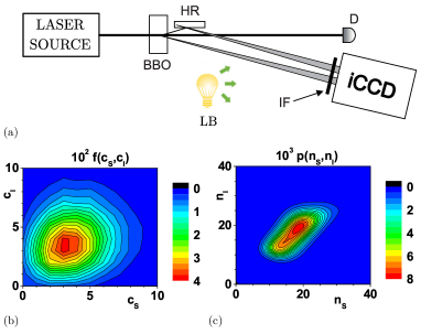
Figure 1: (a) Scheme of the experimental setup: nonlinear crystal BBO producing a TWB; mirror HR reflecting the idler beam; light bulb LB emitting the noisy field with defined intensity uniform over the iCCD; bandpass interference filter IF; intensified CCD camera iCCD; detector D used for pump-beam stabilization. (b) Normalized experimental photocount histogram $f(c_{\rm s},c_{\rm i})$ giving the number of realizations with $c_{\rm s}$ and $c_{\rm i}$ registered electrons (photocounts) and (c) the corresponding reconstructed photon-number distribution $p(n_{\rm s},n_{\rm i})$ of the least-noisy TWB.

In the experiment, we first investigated the TWB without an additional noise. The experimental photocount histogram $f(c_{\rm s},c_{\rm i})$ obtained after $10^{4}$ measurement repetitions as well as the reconstructed photon-number distribution $p(n_{\rm s},n_{\rm i})$ are plotted in Figs. 1(b) and 1(c). This TWB caused on average $\langle c\rangle=5.5$ photocounts per detection region, which corresponds to $\langle n\rangle=\langle W\rangle=24.4$ photon pairs in a TWB. Owing to non-ideal detection efficiency of the iCCD camera the joint photocount distribution $f$ is smeared from the diagonal given as $c_{\rm s}=c_{\rm i}$. The reconstruction tends to eliminate this smearing, but still a typical droplet shape is observed for the photon-number distribution $p$. The maximum-likelihood approach was applied to arrive at the photon-number distribution $p(n_{\rm s},n_{\rm i})$ in the form of a steady state of the following iteration procedure Dempster et al. (1977); Peřina Jr. et al. (2012b) ($l=0,1,\ldots$):

$$p^{(l+1)}(n_{\rm s},n_{\rm i}) = p^{(l)}(n_{\rm s},n_{\rm i})$$ (14)

$$\mbox{}\times\sum_{c_{\rm s},c_{\rm i}}\frac{f(c_{\rm s},c_{\rm i})T_{\rm s}(c_{\rm s},n_{\rm s})T_{\rm i}(c_{\rm i},n_{\rm i})}{\sum_{n^{\prime}_{s},n^{\prime}_{i}}T_{\rm s}(c_{\rm s},n^{\prime}_{\rm s})T_{\rm i}(c_{\rm i},n^{\prime}_{\rm i})p^{(l)}(n^{\prime}_{\rm s},n^{\prime}_{\rm i})}.$$

The positive-operator-valued measures $T_{\rm a}$, $a={\rm s,i}$, characterize detection in the region with beam $a$. We have for an iCCD camera with $N_{a}$ active pixels, detection efficiency $\eta_{a}$ and mean dark count number per pixel $D_{a}$ Peřina Jr. et al. (2012b):

$$T_{a}(c_{a},n_{a}) = \left(\begin{array}[]{c}N_{a}\\ c_{a}\end{array}\right)(1-D_{a})^{N_{a}}(1-\eta_{a})^{n_{a}}(-1)^{c_{a}}$$ (20)

$$\mbox{}\times\sum_{l=0}^{c_{a}}\left(\begin{array}[]{c}c_{a}\\ l\end{array}\right)\frac{(-1)^{l}}{(1-D_{a})^{l}}\left(1+\frac{l}{N_{a}}\frac{\eta_{a}}{1-\eta_{a}}\right)^{n_{a}}.$$

Calibration of our iCCD camera Peřina Jr. et al. (2012a) gave us the following parameters $\eta_{\rm s}=0.230\pm 0.005$, $\eta_{\rm i}=0.220\pm 0.005$, $N_{\rm s}=N_{\rm i}=4096$, $D_{\rm s}N_{\rm s}=D_{\rm i}N_{\rm i}=0.040\pm 0.001$ for the signal (s) and idler (i) detection regions.

IV Non-classicality and entanglement degradation caused by the increasing noise

To investigate degradation of the TWB entanglement as well as to analyze the performance of the above entanglement quantifiers when the noise in the TWB increases, the noise with multi-thermal photon statistics, originating in a bulb lamp, was superimposed equally onto the signal and idler beams. An increasing voltage applied to the bulb lamp leads to the increasing mean photon numbers $\langle n\rangle_{\rm n}$ of the noise field. 36 TWBs with different levels of the noise were analyzed: Their mean photocount numbers $\langle c_{\rm s}\rangle$ and $\langle c_{\rm i}\rangle$ in the signal and idler detection regions, respectively, as well as the mean photocount numbers $\langle c\rangle_{\rm n}$ of the noise field measured in the independent detection are plotted in Fig. 2(a).

We first roughly estimate the amount of non-classicality by applying the noise-reduction-factor $R$ Chesi et al. (2019) in Eq. (1) that, in fact, quantifies the relative amount of paired photons in a TWB. The gradual decrease of the relative amount of paired photons in the measured TWBs with the increasing noise is monitored in Fig. 2(b) by the increasing values of the noise-reduction-factors $R_{\rm c}$ and $R_{\rm n}$ determined from the photocount histograms and reconstructed photon-number distributions of the analyzed TWBs, respectively. According to the graphs in Fig. 2(b), the TWBs with the mean noise photocount numbers $\langle c\rangle_{\rm n}$ smaller than 5 are nonclassical ($R_{\rm c},R_{\rm n}<1$). As the reconstruction algorithm qualitatively preserves the non-classicality while improving it quantitatively, the curves for $R_{\rm c}$ and $R_{\rm n}$ mutually cross at $R=1$ where the transition to the classical region of $R$ occurs.

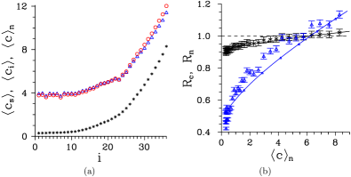
Figure 2: (a) Mean experimental photocount numbers $\langle c_{\rm s}\rangle$ (blue $\triangle$), $\langle c_{\rm i}\rangle$ (red $\circ$) and $\langle c\rangle_{\rm n}$ ($\ast$) in, in turn, signal-beam, idler-beam and noise detection region versus the number $i$ identifying a TWB. (b) Noise-reduction-factors $R_{\rm c}$ ($\ast$) and $R_{\rm n}$ (blue $\triangle$) determined for the experimental photocount histograms and reconstructed photon-number distributions of TWBs, respectively, as they depend on mean noise photocount number $\langle c\rangle_{\rm n}$. Experimental data are plotted as isolated symbols with error bars derived from the number of measurement repetitions. Relative errors in (b) estimated from the data scattering are better than 3 %. In (a), experimental errors are smaller than the plotted symbols. In (b), theoretical solid curves with appropriate symbols originate in the model, dashed line $R=1$ indicates the non-classicality border.

The experimental results for the noisy TWBs are compared with the predictions of the model that convolves the photocount (photon-number) distributions of the independent noisy fields present in both the signal and idler beams with the photocount histogram $f^{\rm n-l}$ (photon-number distribution $p^{\rm n-l}$) of the original TWB without an additional noise using the formula analogous to that in Eq. (8). The distributions of the noisy fields are given by Eq. (9) in which we consider $\langle c\rangle_{\rm n}$ ($\langle n\rangle_{\rm n}=\langle c\rangle_{\rm n}/\eta$) mean photocount numbers (photon numbers) distributed into $N_{\rm c}$ ($N_{\rm n}$) equally populated modes. Comparison with the experimental results suggests $K_{\rm c}=110$ independent modes in the noise fields to explain the loss of non-classicality of the experimental photocount histograms $f$. The slightly smaller number $K_{\rm n}=90$ of independent modes is appropriate in the case of the reconstructed photon-number distributions $p$. This is related to the fact that the reconstruction with the positive-operator-valued measures $T_{\rm a}$ in Eq. (20) partially reduces the noise.

The experimental as well as the theoretical values of both NDs $\tau$ and NCPs $\nu$ drawn for different values of the mean noise photocount number $\langle c\rangle_{\rm n}$ in Fig. 3 confirm the best performance of the NI $M$ in revealing the non-classicality of a whole multi-mode TWB. On the other hand, the NI $E_{3}$ involving the third-order intensity moments gives the worst results, in agreement with the findings of Ref. Peřina Jr. et al. (2017). Whereas the NI $M$ identifies the non-classicality of the TWB up to $\langle c\rangle_{\rm n}\approx 6$, the third-order intensity moments of NI $E_{3}$ lose their ability to reveal the non-classicality around $\langle c\rangle_{\rm n}\approx 4$. It is worth noting that the commonly used noise-reduction factors $R$ perform up to $\langle c\rangle_{\rm n}\approx 5$. The comparison of NCPs $\nu$ drawn in Figs. 3(c,d) with the NDs $\tau$ plotted in Figs. 3(a,b) shows comparable sensitivity of the NCPs in quantification of the non-classicality from the point of view of the experimental errors under our conditions. We note, however, that the NCPs cannot quantify the non-classicality of highly quantum states Peřina Jr. et al. (2019). On the other hand, the intensity moments do not have to be involved et all in the determination of NCPs if the NIs based on the photocount (photon-number) probabilities are applied Peřina Jr. et al. (2017, 2019). In this case the commutation relations, that depend on the number of field’s modes, are not needed. Substantial improvement of the amount of TWB non-classicality after the reconstruction is evident when we compare the NDs $\tau$ and NCPs $\nu$ drawn in Figs. 3(a,c) for the experimental photocount histograms $f$ with those in Figs. 3(b,d) appropriate for the reconstructed photon-number distributions $p$. The increase of non-classicality in the reconstruction is due to partial elimination of the noise and, mainly, correction for the finite detection efficiencies that brake the photon pairs from which the non-classicality originates. The values of NDs $\tau$ and NCPs $\nu$ are around 4-5 times larger after the reconstruction. This factor is roughly proportional to $1/\eta$ which is a signature of the fact that the mean photocount and photon numbers per one mode are smaller or comparable to 1. For stronger fields, the mapping between the NDs $\tau$ (NCPs $\nu$) belonging to the photocount histograms and the reconstructed photon-number distributions is nonlinear (compare the condition $\tau\leq 1/2$).

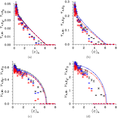
Figure 3: Non-classicality depths $\tau$ (a,b) and non-classicality counting parameters $\nu$ (c,d) for NIs $M$ (black $\ast$), $E_{2}$ (blue $\triangle$) and $E_{3}$ (red $\circ$) for photocount histograms (a,c) and photon-number distributions (b,d) as they depend on mean noise photocount number $\langle c\rangle_{\rm n}$. Experimental data are plotted as isolated symbols with error bars derived from the number of measurement repetitions, solid curves with appropriate symbols come from the model. Relative errors in (a,b) [(c,d)] estimated from the data scattering are better than 10 % [5 %].

The consideration of just one typical (average) mode of a TWB with its intensity moments given along Eqs. (11) and (12) leads to much smaller values of the moments and thus the increased role of the noise. Especially the odd-order moments are affected as the odd-order moments of intensity fluctuations are sign-sensitive. We note that the measured TWBs were composed of typically 50 modes determined by Eq. (10). In our case, this disqualifies the use of third-order moments of the NI $E_{3}$ for quantification of the non-classicality. On the other hand, the negativity $E_{\rm N}$ determined from up-to the second-order intensity moments can directly be used as an entanglement quantifier, as documented in Figs. 4(a,b). Alternatively, it can be considered as another NI and then the corresponding NDs $\tau_{E_{\rm N}}$ [see Figs. 4(c,d)] and NCPs $\nu_{E_{\rm N}}$ can be calculated. In both cases, it identifies the measured TWBs as entangled up to $\langle c\rangle_{\rm n}\approx 6$. The comparison of NDs $\tau_{m}$ and $\tau_{e_{2}}$ [Figs. 4(c,d)] belonging to the NIs $M$ and $E_{2}$ applied to single-mode moments with those valid for the whole TWBs [Figs. 3(a,b)] shows that the low-order single-mode intensity moments successfully maintain the information about the resistance of TWB non-classicality against the noise.

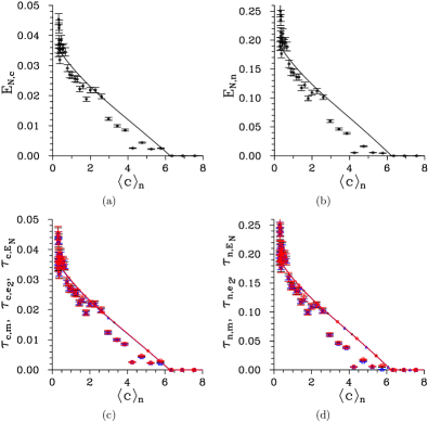
Figure 4: Negativity $E_{\rm N}$ (a,b) and non-classicality depth $\tau$ (c,d) for NIs $M$ (black $\ast$), $E_{2}$ (blue $\triangle$) and $E_{\rm N}$ (red $\circ$) for photocount histograms (a,c) and photon-number distributions (b,d) ’reduced’ to a single-mode along Eq. (12) as they depend on mean noise photocount number $\langle c\rangle_{\rm n}$. Experimental data are plotted as isolated symbols with error bars derived from the number of measurement repetitions, solid curves with appropriate symbols come from the model. Relative errors estimated from the data scattering are better than 10 % for all plotted quantities.

At the end, we note that the error bars plotted in the figures were determined solely from the number of measurement repetitions. As such they do not reflect instabilities and imperfections in the setup occurring during the measurements of TWBs with different levels of the noise (one hour was typically needed to characterize one TWB). Slow pump-beam intensity fluctuations, pump-beam misalignment (temperature-induced position shifts) in the setup, temperature stabilization of the iCCD camera and its synchronization with the laser source were responsible for the main detrimental effects. The corresponding errors were estimated from the experimental points in the graphs of Figs. 2, 3 and 4: Average relative errors were obtained by considering all pairs of neighbor experimental points on a given experimental curve and determining the mean value and the relative declination for each pair.

V Conclusions

We have experimentally investigated deterioration of the entanglement of a twin beam caused by an increasing external noise. We have suggested, verified and mutually compared three experimentally feasible ways for quantifying the twin-beam entanglement. The first two are based upon the non-classicality depths and the non-classicality counting parameters of suitable non-classicality identifiers. In the third way, the negativity is directly determined for one typical mode of the TWB. The three entanglement quantifiers perform comparably. They may be applied in any metrology, quantum-imaging or quantum-information scheme that uses the twin beams and whose sensitivity to the noise has to be quantified.

References

- Migdall (1999) A. Migdall, “Correlated-photon metrology without absolute standards,” Physics Today 52, 41—46 (1999).
- Peřina Jr. et al. (2012a) J. Peřina Jr., O. Haderka, M. Hamar, and V. Michálek, “Absolute detector calibration using twin beams,” Opt. Lett. 37, 2475—2477 (2012a).
- Nielsen and Juang (2000) M. A. Nielsen and I. L. Juang, Quantum Computation and Quantum Information (Cambridge Univ. Press, Cambridge, 2000).
- Magańa-Loaiza et al. (2019) O. S. Magańa-Loaiza, R. de J. León-Montiel, A. Perez-Leija, A. B. U Ren, C. You, K. Busch, A. E. Lita, S. W. Nam, R. P. Mirin, and T. Gerrits, “Multiphoton quantum-state engineering using conditional measurements,” npj Quant. Inf. 5, 80 (2019).
- Allevi and Bondani (2018) A. Allevi and M. Bondani, “Can nonclassical correlations survive in the presence of asymmetric lossy channels?” Eur. Phys. J. D 18, 178 (2018).
- Leonhardt (1997) U. Leonhardt, Measuring the Quantum State of Light (Cambridge University Press, Cambridge, 1997).
- Lvovsky and Raymer (2009) A. I. Lvovsky and M. G. Raymer, “Continuous-variable optical quantum state tomography,” Rev. Mod. Phys. 81, 299—332 (2009).
- Duan et al. (2000) L.-M. Duan, G. Giedke, J. I. Cirac, and P. Zoller, “Inseparability criterion for continuous variable systems,” Phys. Rev. Lett. 84, 2722—2725 (2000).
- Simon (2000) R. Simon, “Peres-Horodecki separability criterion for continuous variable systems,” Phys. Rev. Lett. 84, 2726—2729 (2000).
- Shchukin et al. (2005) E. Shchukin, T. Richter, and W. Vogel, “Nonclassicality criteria in terms of moments,” Phys. Rev. A 71, 011802(R) (2005).
- Miranowicz et al. (2010) A. Miranowicz, M. Bartkowiak, X. Wang, Y.-X. Liu, and F. Nori, “Testing nonclassicality in multimode fields: A unified derivation of classical inequalities,” Phys. Rev. A 82, 013824 (2010).
- Gerke et al. (2015) S. Gerke, J. Sperling, W. Vogel, Y. Cai, J. Roslund, N. Treps, and C. Fabre, “Full multipartite entanglement of frequency-comb gaussian states,” Phys. Rev. Lett. 114, 050501 (2015).
- Harder et al. (2016) G. Harder, T. J. Bartley, A. E. Lita, S. W. Nam, T. Gerrits, and C. Silberhorn, “Single-mode parametric-down-conversion states with 50 photons as a source for mesoscopic quantum optics,” Phys. Rev. Lett. 116, 143601 (2016).
- Mandel and Wolf (1995) L. Mandel and E. Wolf, Optical Coherence and Quantum Optics (Cambridge Univ. Press, Cambridge, 1995).
- Boyd (2003) R. W. Boyd, Nonlinear Optics, 2nd edition (Academic Press, New York, 2003).
- Glauber (1963) R. J. Glauber, “Coherent and incoherent states of the radiation field,” Phys. Rev. 131, 2766—2788 (1963).
- Peřina (1991) J. Peřina, Quantum Statistics of Linear and Nonlinear Optical Phenomena (Kluwer, Dordrecht, 1991).
- Peřina Jr. et al. (2017) J. Peřina Jr., I. I. Arkhipov, V. Michálek, and O. Haderka, “Non-classicality and entanglement criteria for bipartite optical fields characterized by quadratic detectors,” Phys. Rev. A 96, 043845 (2017).
- Arkhipov and Peřina Jr (2018) I. I. Arkhipov and J. Peřina Jr, “Experimental identification of non-classicality of noisy twin beams and other related two-mode states,” Sci. Rep. 8, 1460 (2018).
- Arkhipov et al. (2016) I. I. Arkhipov, J. Peřina Jr., V. Michálek, and O. Haderka, “Experimental detection of nonclassicality of single-mode fields via intensity moments,” Opt. Express 24, 29496—29505 (2016).
- Haderka et al. (2005) O. Haderka, J. Peřina Jr., and M. Hamar, “Simple direct measurement of nonclassical joint signal-idler photon-number statistics and correlation area of twin photon beams,” J. Opt. B: Quantum Semiclass. Opt. 7, S572—S576 (2005).
- Allevi et al. (2012) A. Allevi, S. Olivares, and M. Bondani, “Measuring high-order photon-number correlations in experiments with multimode pulsed quantum states,” Phys. Rev. A 85, 063835 (2012).
- Peřina Jr. et al. (2013) J. Peřina Jr., O. Haderka, V. Michálek, and M. Hamar, “State reconstruction of a multimode twin beam using photodetection,” Phys. Rev. A 87, 022108 (2013).
- Chesi et al. (2019) G. Chesi, L. Malinverno, A. Allevi, R. Santoro, M. Caccia, and M. Bondani, “Measuring nonclassicality with silicon photomultipliers,” Opt. Lett. 44, 1371—1374 (2019).
- Klyshko (1996) D. N. Klyshko, “Observable signs of nonclassical light,” Phys. Lett. A 213, 7—15 (1996).
- Waks et al. (2006) E. Waks, B. C. Sanders, E. Diamanti, and Y. Yamamoto, “Highly nonclassical photon statistics in parametric down-conversion,” Phys. Rev. A 73, 033814 (2006).
- Wakui et al. (2014) K. Wakui, Y. Eto, H. Benichi, S. Izumi, T. Yanagida, K. Ema, T. Numata, D. Fukuda, M. Takeoka, and M. Sasaki, “Ultrabroadband direct detection of nonclassical photon statistics at telecom wavelength,” Sci. Rep. 4, 4535 (2014).
- Lee (1991) C. T. Lee, “Measure of the nonclassicality of nonclassical states,” Phys. Rev. A 44, R2775—R2778 (1991).
- Peřina Jr. et al. (2019) J. Peřina Jr., O. Haderka, and V. Michálek, “Simultaneous observation of higher-order non-classicalities based on experimental photocount moments and probabilities,” Sci. Rep. 9, 8961 (2019).
- Adesso and Illuminati (2007) G. Adesso and F. Illuminati, “Entanglement in continuous variable systems: Recent advances and current perspectives,” J. Phys. A: Math. Theor. 40, 7821—7880 (2007).
- Arkhipov et al. (2015) I. I. Arkhipov, J. Peřina Jr., J. Peřina, and A. Miranowicz, “Comparative study of nonclassicality, entanglement, and dimensionality of multimode noisy twin beams,” Phys. Rev. A 91, 033837 (2015).
- Hill and Wootters (1997) S. Hill and W. K. Wootters, “Computable entanglement,” Phys. Rev. Lett. 78, 5022 (1997).
- Peres (1996) A. Peres, “Separability criterion for density matrice,” Phys. Rev. Lett. 77, 1413 –1415 (1996).
- Horodecki et al. (1996) M. Horodecki, P. Horodecki, and R. Horodecki, “Separability of mixed states: Necessary and sufficient conditions,” Phys. Lett. A 223, 1 –8 (1996).
- Saleh (1978) B. E. A. Saleh, Photoelectron Statistics (Springer-Verlag, New York, 1978).
- Gradshtein and Ryzhik (2000) I. S. Gradshtein and I. M. Ryzhik, Table of Integrals, Series, and Products, 6th ed. (Academic Press, San Diego, 2000).
- Peřina and Křepelka (2011) J. Peřina and J. Křepelka, “Joint probability distributions and entanglement in optical parametric processes,” Opt. Commun. 284, 4941—4950 (2011).
- Dempster et al. (1977) A. P. Dempster, N. M. Laird, and D. B. Rubin, “Maximum likelihood from incomplete data via the EM algorithm,” J. R. Statist. Soc. B 39, 1—38 (1977).
- Peřina Jr. et al. (2012b) J. Peřina Jr., M. Hamar, V. Michálek, and O. Haderka, “Photon-number distributions of twin beams generated in spontaneous parametric down-conversion and measured by an intensified CCD camera,” Phys. Rev. A 85, 023816 (2012b).