Dual Graph Embedding for Object-Tag Link Prediction on the Knowledge Graph

Abstract

Knowledge graphs (KGs) composed of users, objects, and tags are widely used in web applications ranging from E-commerce, social media sites to news portals. This paper concentrates on an attractive application which aims to predict the object-tag links in the KG for better tag recommendation and object explanation. When predicting the object-tag links, both the first-order and high-order proximities between entities in the KG propagate essential similarity information for better prediction. Most existing methods focus on preserving the first-order proximity between entities in the KG. However, they cannot capture the high-order proximities in an explicit way, and the adopted margin-based criterion cannot measure the first-order proximity on the global structure accurately. In this paper, we propose a novel approach named Dual Graph Embedding (DGE) that models both the first-order and high-order proximities in the KG via an auto-encoding architecture to facilitate better object-tag relation inference. Here the dual graphs contain an object graph and a tag graph that explicitly depict the high-order object-object and tag-tag proximities in the KG. The dual graph encoder in DGE then encodes these high-order proximities in the dual graphs into entity embeddings. The decoder formulates a skip-gram objective that maximizes the first-order proximity between observed object-tag pairs over the global proximity structure. With the supervision of the decoder, the embeddings derived by the encoder will be refined to capture both the first-order and high-order proximities in the KG for better link prediction. Extensive experiments on three real-world datasets demonstrate that DGE outperforms the state-of-the-art methods.

I Introduction

In Web applications such as E-commerce and social media sites, many recommender systems incorporate the knowledge graph (KG) composed of users, objects, and tags to provide accurate and explainable recommendation [1]. This paper focus on an attractive application which aims to predict the object-tag links in this kind of KG for better tag recommendation [2] and object management [3].

In the object-tag link prediction problem, the knowledge graph contains three types of entities (i.e., users, objects, and tags) and two types of relations (i.e., Interact and TaggedWith) as Fig. 1 shows. Two types of (head, relation, tail) triplets with the forms of (user, Interact, object) and (object, TaggedWith, tag) are included in the KG. In particular, this task focuses on the latter type of triplets by taking the objects as the heads and the tags as the tails to predict. Here both the first-order and high-order proximities in the KG provide structural similarity information to enhance the link prediction. At first, the first-order proximity between a head-tail pair determines the existence of the corresponding link directly. In Fig. 1, the object and the tag that are associated by an observed link of type $r_{2}$ share the stronger first-order proximity than the nodes that are not directly linked. The existing first-order proximity information in these observed links can discover new links between objects and tags that share high proximity. Besides the first-order proximity, the high-order object-object and tag-tag proximities implied in the high-order connectivities in the KG provide collaborative signals for link prediction. More specifically, the high-order proximity between two objects encourages one of the objects to link to the tags of the other one. Similarly, the high-order proximity between two tags enriches the links for the object linked to any one of these tags. For example, in Fig. 1, $o_{1}$ and $o_{3}$ are two-hop neighbors on the path $o_{1}\xrightarrow{-r_{1}}u_{2}\xrightarrow{r_{1}}o_{3}$, and they share high-order proximity. Then $t_{4}$ that is linked to $o_{3}$ may be also relevant to $o_{1}$. Similarly, the tag $t_{2}$ of $o_{1}$ shares the high-order proximity with $t_{3}$ over the path $t_{2}\xrightarrow{-r_{2}}o_{2}\xrightarrow{r_{2}}t_{3}$, and a link between $o_{1}$ and $t_{3}$ is probable to be added. In this sense, both the first-order and high-order proximities in the KG need to be captured for high-quality link prediction.

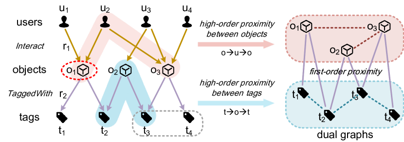
Figure 1: A toy example of the KG in the object-tag link prediction task. The purple lines indicate the first-order object-tag proximity. The high-order proximity exists between the objects in the left red region. Tags in the left blue region also share the high-order proximity. These high-order proximities are depicted in the dual graphs shown on the right side. $o_{1}$ with the red circle is the head whose tails need to be predicted. Tags in the grey circle are discovered by high-order relationships in the KG.

However, existing models fail to capture both the first-order and high-order proximities in the KG jointly. Translational distance models designed for KG completion measure the distances between entities and their immediate neighbors after the translations carried by the relations [4, 5, 6]. In this way, these models concentrate on the first-order proximity between existing triplets [7]. Some other methods based on random walk [8] or feature aggregation [9, 10] on the KG focus on the information propagation from current entity to its directly linked entity. Without capturing the high-order proximities explicitly, these methods will lose the collaborative information in the high-order connectivities in the KG, which is essential for prediction with high accuracy. For example, $t_{3}$ and $t_{4}$ in Fig. 1 may be overlooked by these methods when predicting the tails of $o_{1}$. Besides, the margin-based criterion commonly used in the KG completion methods only considers the pairwise relations between heads and tails, which may fail to depict the first-order proximity between any pair of entities over the global proximity structure.

In this paper, we propose a Dual Graph Embedding (DGE) model in an auto-encoding architecture that simultaneously captures the first-order and high-order proximities in the KG to predict the missing object-tag links. Here the dual graphs contain an object graph and a tag graph constructed based on the high-order connectitities in the KG. Hence links in the dual graphs describe the high-order object-object and tag-tag proximities explicitly. The dual graph encoder in DGE then captures these high-order proximities by encoding the structural information in the dual graphs into entity embeddings. In the decoder, instead of the widely-used margin loss, we formulate a skip-gram objective that maximizes the likelihood that each observed tag is relevant to a given object over all the possible tags. In this way, the decoder measures the first-order proximity in the global proximity structure in the KG and refines the embeddings learned from the encoder. The auto-encoding formulation encourages DGE to capture the first-order and high-order proximities in an end-to-end manner for better prediction. We conduct our experiments on several real-world datasets for tag recommendation tasks. The results show that DGE predicts high-relevant object-tag pairs compared to the state-of-the-art methods. Our contributions could be summarized as follows:

• We propose a Dual Graph Embedding (DGE) method to capture both the first-order and high-order proximities in the KG simultaneously, and further improve the quality of the object-tag link prediction;

• We adopt the skip-gram objective that maximizes the likelihood of the observed tags given an object over the candidate tag set, and the first-order proximity between each object-tag pair in the global proximity structure can be measured more accurately;

• Extensive experiments are conducted on three real-world datasets for tag recommendation. The empirical results show that our method outperforms the state-of-the-art methods on relevant tag prediction for target objects.

II Related Work

II-A Knowledge Graph Completion

Considering the incompleteness of knowledge graphs, many methods have been proposed to add new triplets to the knowledge graph. A typical task of KG completion is link prediction, which is widely applied to recommender systems in real-life scenarios [7].

Many translational distance models learn low-dimension embeddings of entities and relations by minimizing the distance between two directly linked entities in a translated space [11]. Besides, they adopt the margin-based criterion to measure the first-order proximity in the KG. TransE [4] treats relations as translations from heads to tails. This method supposes that the added result of the head and relation embeddings should be close to the tail embedding. To follow up, TransH [5] modifies the scoring function by projecting entities and relations into a hyperplane. TransR [6] introduces relation-specific spaces and projects the head and tail embeddings into the corresponding space. To simplify TransR, TransD [12] replaces the projection matrix into the product of two mapping vectors. Besides, some methods like KG2E [13] and TransG [14] redefine the distance by assuming that the entity and relation embeddings are from Gaussian distributions.

II-B Tag Recommendation

Tag recommendation methods can be formulated as the link prediction problem on the user-object-tag relation graph [2].

Some matrix factorization (MF) based methods model the pairwise relationships among users, objects and tags to learn the low-dimension embeddings [15]. Other methods additionally extract the tag co-occurrences and model the tag-tag proximity to recommend relevant tags for certain objects [16, 17]. Some recent methods employ the random walk with restart or node feature aggregation scheme in the input graph to predict the link between object nodes and tag nodes [8, 9, 10]. Although they consider the high-order connectivities in the input graph, they focus on the information propagation process between two directly linked nodes.

In summary, methods for KG completion and tag recommendation cannot capture the collaborative signals from the high-order object-object and tag-tag proximities in the KG explicitly. Besides, the margin loss employed for KG completion cannot measure the first-order proximity over the global proximity structure accurately.

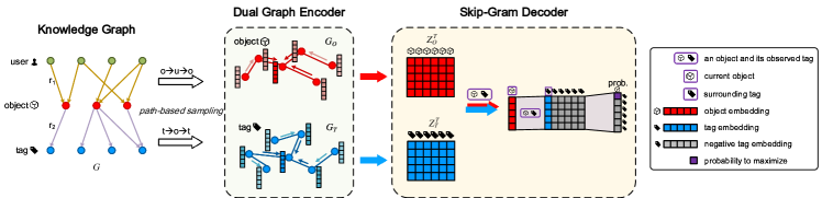
Figure 2: The Dual Graph Embedding model for the prediction of the object-tag links. We adopt the path-based sampling scheme to construct the object and tag graphs that contain the high-order proximities. A dual graph encoder contains two 2-layer GCN architectures to embed the object-object and tag-tag proximities. The decoder measures the first-order proximity between objects and tags, and uses the skip-gram objective to supervise the encoder.

III Preliminary

III-A Problem Definition

In the object-tag link prediction task, we first introduce the input knowledge graph and the task goal.

Knowledge graph in this task. We denote the knowledge graph in this task as $G=\{(h,r,t)|h,t\in\mathcal{E},r\in\mathcal{R}\}$, where $\mathcal{E}=\mathcal{U}\cup\mathcal{O}\cup\mathcal{T}$. Here $\mathcal{U}=\{u_{1},u_{2},\cdots,u_{P}\}$, $\mathcal{O}=\{o_{1},o_{2},\cdots,o_{N}\}$, and $\mathcal{T}=\{t_{1},t_{2},\cdots,t_{M}\}$ are the user, object and tag set with $P$, $M$, and $N$ entities respectively. The relation set $\mathcal{R}$ is composed of two types of relations including $r_{1}=Interact$ and $r_{2}=TaggedWith$ as Fig. 1 shows.

Task description. Given the input $G$, we aim to predict the existence of the object-tag link between any pair in $\{(h,t)|h\in\mathcal{O},t\in\mathcal{T}\}$. Here objects are considered as given heads and tags are treated as candidate tails to predict. In particular, we denote the observed tag set of a given object $o_{i}$ as $\mathcal{S}_{o_{i}}=\{t^{i}_{1},t^{i}_{2},...,t^{i}_{M_{i}}\}$, where $\mathcal{S}_{o_{i}}$ contains $M_{i}$ observed tags linked to $o_{i}$ and $\mathcal{S}_{o_{i}}\subset\mathcal{T}$.

III-B Terminology Explanation

We give formal definitions of some important terminologies related to this task:

High-order connectivity. We take the definition given in [1] that the $L$-order connectivity means the long range path $e_{0}\xrightarrow{r^{1}}e_{1}\xrightarrow{r^{2}}\cdots\xrightarrow{r^{L}}e_{L}$, where $e_{i}\in\mathcal{E}$ and $r^{j}\in\mathcal{R}$ for $i=0,\cdots,L$ and $j=1,\cdots,L$. Then $e_{L}$ is the $L$-hop neighbor of $e_{0}$.

Path-based neighbors. According to the high-order connectivities, we consider a predefined path set $\mathcal{P}=\{e_{0}\xrightarrow{r^{1}}\cdots\xrightarrow{r^{L}}e_{L}\}$ by fixing the types of all the entities and relations as well as forcing $e_{0}$ and $e_{L}$ to be the same types. Then for any path $pa\in\mathcal{P}$, the start and end entities are $\mathcal{P}$-path-based neighbors of each other.

High-order object-object and tag-tag proximities. The high-order proximity exists between an entity and its path-based neighbor given a predefined $\mathcal{P}$. We focus on the proximities existing in objects and tags since this task only predicts the missing object-tag links. Given an object $o_{i}$, $o_{i}$ and $o_{j}$ share high-order proximity if $o_{j}$ is a path-based neighbor of $o_{i}$. The high-order tag-tag proximity can be defined in the same way.

IV Proposed Model

IV-A Model Overview

Our proposed DGE consists of a dual graph encoder and a skip-gram decoder, and the model framework is depicted in Fig. 2. The dual graphs here indicate an object graph and a tag graph containing the high-order object-object and tag-tag proximities in the KG respectively. The encoder then extracts both the high-order proximities from the dual graphs and embeds them into entity embeddings. Besides, the skip-gram decoder measures the first-order proximity over the global proximity structure in the KG to determine the existence of links and to supervise the entire model.

According to the high-order connectivities in the input KG, we can sample the path-based neighbors of objects and tags respectively. These extracted neighboring correlations that contain the high-order proximities are utilized to build the object graph $G_{O}=(V_{O},E_{O})$ and the tag graph $G_{T}=(V_{T},E_{T})$, where $V_{T}$ and $E_{T}$ denote the vertex set and link set of tags (similarly, $V_{O}$ and $E_{O}$ are for objects). Both graphs form the dual graphs, where we assume that the directional information in the initial KG is not important in this task. Then the encoder extracts the high-order object-object and tag-tag proximities from the dual graphs $G_{O}$ and $G_{T}$ respectively. The encoded object and tag embeddings are given by

$$Z_{O},Z_{T}=DGEnc(G_{O},G_{T}),$$ (1)

where $Z_{O}\in\mathbb{R}^{N\times d}$ and $Z_{T}\in\mathbb{R}^{M\times d}$ are the object and tag embeddings respectively with the latent dimension $d$, and $DGEnc$ denotes the encoding process.

In the decoder, for an object $o_{i}$, we assume that the observed tags in $\mathcal{S}_{o_{i}}$ share the stronger first-order proximity with $o_{i}$ compared to those globally unobserved ones. Actually, this assumption is consistent with the idea of the skip-gram model [18] that the surrounding words are more related to the current word compared to those globally distant words. In this sense, to capture the dominant proximity information in the global structure for any $o_{i}$, we formulate the decoder from the skip-gram perspective. More specifically, given any pair $(o_{i},t_{j})$, the current object vector is the $i$th row of $Z_{O}$ denoted by $Z_{O,i}$ and the target tag vector is the $j$th row of $Z_{T}$ denoted by $Z_{T,j}$. Here $Z_{T}$ is taken as the candidate surrounding tag embedding matrix. Then the decoder calculates the probability $p(t_{j}|o_{i})$ that $t_{j}$ is linked to $o_{i}$ in the same way as the skip-gram model based on the indexed and candidate vectors,

$$p(t_{j}|o_{i})=SGDec(Z_{O,i},Z_{T,j}),$$ (2)

where $SGDec$ implies the skip-gram decoding process. To supervise the whole model, for the current $o_{i}$, the skip-gram objective [18] maximizes the likelihood of its $M_{i}$ observed surrounding tags in $\mathcal{S}_{o_{i}}$, which is given by

$$\max p(t^{i}_{1},t^{i}_{2},\cdots,t^{i}_{M_{i}}|o_{i})$$

$$= \max\prod_{m=1}^{M_{i}}p(t^{i}_{m}|o_{i}),$$ (3)

$$= \max\prod_{m=1}^{M_{i}}SGDec(DGEnc(G_{O},G_{T})[o_{i},t^{i}_{m}]).$$

During the training process, $Z_{O}$ and $Z_{T}$ will be refined to capture more similarity information from both the first-order and high-order proximities in the KG to assist the prediction.

IV-B Dual Graph Encoder

Since the high-order proximities in the input knowledge graph $G$ propagate essential information for link prediction, we introduce a dual graph encoder to capture these proximities. More specifically, we construct the dual graphs including the object graph $G_{O}=(V_{O},E_{O})$ and the tag graph $G_{T}=(V_{T},E_{T})$ via a path-based neighbor sampling scheme on the input graph $G$. Thus links in both graphs illustrate the high-order proximities in the input $G$. Then the dual graph encoder embeds the structural information of $G_{O}$ and $G_{T}$ into the embeddings $Z_{O}$ and $Z_{T}$. In this way, $Z_{O}$ and $Z_{T}$ fetch the two types of high-order proximities to provide collaborative signals for the subsequent decoder to predict the object-tag links. The internal layout of the encoder is given in Fig. 2.

Encode the high-order proximity between objects. In this process, we encode the object graph $G_{O}$ to mine the high-order proximity between objects. We consider the path set $\mathcal{P}_{o}=\{o_{i}\xrightarrow{-r_{1}}u_{k}\xrightarrow{r_{1}}o_{j}|o_{i},o_{j}\in\mathcal{O},u_{k}\in\mathcal{U}\}$ in the input $G$, and the $\mathcal{P}_{o}$-path-based neighbors can be sampled for each object node. Note that the path set $\mathcal{P}_{o}^{\prime}=\{o_{i}\xrightarrow{r_{2}}t_{k}\xrightarrow{-r_{2}}o_{j}|o_{i},o_{j}\in\mathcal{O},t_{k}\in\mathcal{T}\}$ is not selected since the information propagated on $\mathcal{P}_{o}^{\prime}$ can be captured when representing the tag graph. Accordingly, $G_{O}$ is constructed by adding the link between each pair of the sampled object nodes. To depict the semantic similarities between any two nodes, we utilize Sparse Positive PMI (SPPMI) [19] values which are commonly used in NLP tasks to normalize the link weights of $G_{O}$. Then we denote the corresponding adjacency matrix as $A_{O}\in\mathbb{R}^{N\times N}$.

Considering the superior performance of Graph Convolutional Networks (GCNs) [20] on capturing relations between nodes, we apply a two-layer GCN to encode the object graph’s information into $Z_{O}$. When the content features $X_{O}\in\mathbb{R}^{N\times d_{in}}$ with the feature dimension of $d_{in}$ are provided, GCN can extract the information from both the graph topological structure and the input features. Otherwise, the content features are one-hot encodings in $N$ dimension and $X_{O}$ equals to the $N$-by-$N$ unit matrix $I_{N}$. GCN still represents the structural information at this time. Since the datasets contain no specific content features, we adopt one-hot encodings as the node features in our experiments. Thus, the two-layer GCN encoder for $G_{O}$ is given by

$$Z_{O}=\hat{A}_{O}\mathrm{ReLU}(\hat{A}_{O}X_{O}W_{O}^{(0)})W_{O}^{(1)},$$ (4)

where the normalized $\hat{A}_{O}=\bar{D}_{O}^{-\frac{1}{2}}\bar{A}_{O}\bar{D}_{O}^{-\frac{1}{2}}$ with $\bar{A}_{O}=A_{O}+I_{N}$ and $\bar{D}_{O(ii)}=\sum_{j}\bar{A}_{O(ij)}$. Besides, $W_{O}^{(0)}\in\mathbb{R}^{d_{in}\times h}$ and $W_{O}^{(1)}\in\mathbb{R}^{h\times d}$ are weight matrices for the first and second layers of GCN respectively. $Z_{O}\in\mathbb{R}^{N\times d}$ is the output object embedding matrix representing the local graph structure and the node features if provided. Being split by rows, $Z_{O}=\{Z_{O,i},i=1,\cdots,N\}$ is then fed to the decoder for prediction.

Encode the high-order proximity between tags. Similarly, we encode the tag graph $G_{T}$ to extract the high-order proximity between tags. $G_{T}$ is constructed based on the $\mathcal{P}_{t}$-path-based neighbor sampling process, where $\mathcal{P}_{t}$ in the input $G$ is defined as $\{t_{i}\xrightarrow{-r_{2}}o_{k}\xrightarrow{r_{2}}t_{j}|t_{i},t_{j}\in\mathcal{T},o_{k}\in\mathcal{O}\}$. The link weight between each pair of tag nodes in $G_{T}$ is determined by the SPPMI value of them, and the adjacency matrix $A_{T}\in\mathbb{R}^{M\times M}$ is composed of all the SPPMI values. Then the high-order proximity between tags are encoded into tag embeddings via another two-layer GCN encoder,

$$Z_{T}=\hat{A}_{T}\mathrm{ReLU}(\hat{A}_{T}W_{T}^{(0)})W_{T}^{(1)},$$ (5)

where $\hat{A}_{T}$ is normalized in the same way as $\hat{A}_{O}$, and $W_{T}^{(0)}\in\mathbb{R}^{M\times h}$, $W_{T}^{(1)}\in\mathbb{R}^{h\times d}$ are weight matrices of GCN layers. Since no certain features for tags are provided, we omit the input features $X_{T}$ here. $Z_{T}\in\mathbb{R}^{M\times d}$ is the output tag representation capturing the proximity structure of tag graph. $Z_{T}=\{Z_{T,j},j=1,\cdots,M\}$ are considered as all candidate surrounding tag embeddings for any objects in the decoder.

IV-C Skip-Gram Decoder

In the skip-gram decoder, we measure the first-order proximity between objects and tags over the global proximity structure to predict the missing object-tag links. Besides, for each object, the decoder maximizes the likelihood of the corresponding observed tags to supervise the entire model. The decoding process is shown in Fig. 2.

Given the object embeddings $Z_{O}$ and the tag embeddings $Z_{T}$, the first-order proximity between the current $o_{i}$ and the target $t_{j}$ is measured by the inner product of their corresponding embeddings, i.e., the relevance score is

$$s(o_{i},t_{j})={(Z_{T,j})}^{T}Z_{O,i},$$ (6)

where $Z_{O,i}$ and $Z_{T,j}$ are indexed from $Z_{O}$ and $Z_{T}$ respectively. The probability $p(t_{j}|o_{i})$ for $t_{j}$ and $o_{i}$ is then calculated by applying the softmax operation over the candidate set [18],

$$p(t_{j}|o_{i})=\mathrm{softmax}\left(s(o_{i},t_{j})\right)=\frac{\exp s(o_{i},t_{j})}{U(o_{i})},$$ (7)

where $U(o_{i})=\sum_{k=1}^{M}\exp({(Z_{T,k})}^{T}Z_{O,i})$ represents the normalization factor of $o_{i}$. Here $U(o_{i})$ contains the global proximity information for the head $o_{i}$.

During the optimization process, the probabilities in (IV-A) can be calculated by (7). By maximizing the likelihood for all the cases of each object with its observed tag set, the object and tag embeddings will be refined to get more similarity information from the first-order and high-order proximities to improve the prediction accuracy.

Sub-sampling. In the training process, we calculate the probability in (7) for every observed object-tag pair. Unfortunately calculating (7) requires normalizing over the entire $\mathcal{T}$, which means that it is prohibitively expensive to train the model. Inspired by a sub-sampling scheme of noise-contrastive estimation (NCE) which is widely used in word embedding models [21], we employ NCE to achieve fast training. This scheme trains a binary classifier with label $y$ treating observed tags from data distribution $P_{d}^{o_{i}}$ as positive samples ($y=1$) and tags from a noise distribution $P_{n}$ as negative ones ($y=0$) given $o_{i}$. Assuming that the negative samples appear $K$ times more frequently than the positive ones, the probability that a given tag $t_{j}$ being a positive tag for $o_{i}$ is

$$p(y=1|t_{j},o_{i}) =\frac{p(t_{j}|o_{i})}{p(t_{j}|o_{i})+Kp_{n}(t_{j})}$$ (8)

$$\xrightarrow{\mathrm{omit}\,U(o_{i})} =\frac{\exp s(o_{i},t_{j})}{\exp s(o_{i},t_{j})+Kp_{n}(t_{j})},$$

where $p_{n}(t_{j})$ means $t_{j}$ from noise distribution, and the unnormalized model with a scaled noise distribution by ignoring $U(o_{i})$ in (7) can be normalized during training [21]. Hence, the probability of $t_{j}$ being a negative sample for $o_{i}$ is $p(y=0|t_{j},o_{i})=1-p(y=1|t_{j},o_{i})$. Being consistent with the objective in (IV-A), the goal is converted to maximize the likelihood for the correct labels $y$, averaged over the positive and negative data sets. For $o_{i}$, the log-likelihood is

$$\mathcal{J}_{\Theta}(o_{i})= E_{P_{d}^{o_{i}}}[\log p(y=1|t_{j},o_{i})]$$

$$+ KE_{P_{n}}[\log p(y=0|t_{j},o_{i})]$$ (9)

$$\approx \log p(y=1|t_{j},o_{i})+\sum_{k=1}^{K}\log p(y=0|t_{k},o_{i}).$$

Here the expectations over the data and noise distributions are approximated by sampling during training [21]. Then the overall objective is the summation of the likelihood for all the objects, and the optimization goal can be presented as

$$\max_{\Theta}\sum_{o_{i}\in\mathcal{O}}\mathcal{J}_{\Theta}(o_{i}),$$ (10)

where $\mathcal{J}_{\Theta}(o_{i})$ is obtained by (9). Here the optimization parameters $\Theta=\{W_{O}^{(0)},W_{O}^{(1)},W_{T}^{(0)},W_{T}^{(1)}\}$ determine the encoder, namely the embedding process of the high-order object-object and tag-tag proximities.

TABLE I: summary Statistics of Three Datasets

	Movielens-1M	LastFm	Steam
#objects	3,883	17,632	9,373
#tags	1,008	11,946	352
#users	6,040	1,892	101,654
$\#r_{1}$ (Interact)	1,000,209	70,297	1,100,628
density of u-o interactions	4.2647%	0.2108%	0.1155%
sparsity of object graph	4.5047%	0.8492%	0.3505%
$\#r_{2}$ (TaggedWith)	15,498	108,437	83,700
density of o-t observations	0.3969%	0.0515%	2.5369%
sparsity of tag graph	3.2675%	0.7061%	3.8820%

TABLE II: Experimental Settings ($k_{O}$ and $k_{T}$ control the sparsity of SPPMI matrices of object and tag graph respectively.)

Methods	Settings
MF	hidden size $d=100$
TransE	hidden size $d=100$
TransH	hidden size $d=100$
TransR	hidden size of entities $d_{e}=100$, hidden size of relations $d_{r}=100$
Skip-Gram	hidden size $d=100$
CoFactor	Movielen, Steam: $k$ for SPPMI$=1$, $d=16$;
	LastFM: $k=2$, $d=64$
MAD	$\mu_{1}=\mu_{3}=1$, $\mu_{2}=1e-4$
HeteLearn	$\alpha=0.8$
GCMC+,	Movielen, Steam network structure: $\{128,128,128\}$;
NGCF+	LastFM neitwork structure: $\{64,64,64,64\}$;
	batch size=64, epochs=300, learning rate=2e-3,
	15 negative samples for each positive one,
DGE	Movielen: $k_{O}=0.1,k_{T}=1$, 2-layer GCN structure: $\{32,16\}$;
	LastFM: $k_{O}=1,k_{T}=1$, 2-layer GCN structure: $\{64,64\}$;
	Steam: $k_{O}=5,k_{T}=5$, 2-layer GCN structure: $\{32,16\}$;

V Experiments

V-A Datasets

We adopt three real-world tag recommendation datasets including Movielens-1M, LastFm and Steam to evaluate our model. We summarize the statistical information in Table I.

• Movielens-1M: 3,883 movies are rated by 6,040 users. Tags of each movie are chosen from all 1,008 tags. A total of 15,498 object-tag interactions are observed.

• LastFm: 17,632 artists are listened and tagged by 1,892 users, and the tags are from a tag set with a size of 11,946. In total, 108,437 object-tag observations are included.

• Steam: 9,373 apps are reviewed by 101,654 users. The size of the tag set is 352 and 83,700 object-tag pairs are observed.

V-B Baseline Methods.

To demonstrate the effectiveness of the proposed DGE, we compare DGE with five methods only modeling the first-order proximity and five methods additionally modeling part of the high-order proximities.

V-B1 Methods based on the first-order proximity

The five baseline models developed for the object-tag link prediction includes MF [22], Skip-Gram [21], TransE [4], TransH [5], and TransR [6]. MF factorizes the object-tag interaction matrix into two low-dimension feature matrix for objects and tags. It employs the mean square error (MSE) as the loss function. The skip-gram model adopts the same way as MF to generate features, but it utilizes NCE loss to measure the first-order proximity. The latter three methods treat the relation embeddings as the translation embeddings and define the distance via different scoring functions. They use the margin loss in the training process. In this task, to avoid the bias to irrelevant links in the KG, we adopt the same way as [23] to add an extra Bayesian personalized ranking loss to narrow the translation distance between the related objects and tags.

V-B2 Methods utilizing part of the high-order proximities

We use five methods that model part of the high-order proximities as the comparison methods involving CoFactor [17], MAD [24], HeteLearn [8], GCMC [9] and NGCF [10]. CoFactor based on MF and tag co-occurrences only considers the high-order proximity between tags in the KG. MAD conducts label propagation on the object graph that reflects the object-object proximity. HeteLearn is a state-of-the-art method which provides tags via the random walk scheme on the user-object-tag graph. GCMC and NGCF predict links in the bipartite graph based on node feature aggregation. Since they do not distinguish node types during feature aggregation, we extend them to the user-object-tag tripartite graph denoted by GCMC+ and NGCF+.

TABLE III: $Recall@k$, $NDCG@k$ on Movielens-1M, LastFM, and Steam based on Different Methods

Datasets	Methods	Recall@3	NDCG@3	Recall@5	NDCG@5
	MF	0.7252	0.4116	0.7819	0.3088
	TransE	0.7292	0.4125	0.7776	0.3085
	TransH	0.7293	0.4127	0.7760	0.3081
	TransR	0.6496	0.3390	0.7227	0.2597
	Skip-Gram	0.7467	0.4209	0.7895	0.3144
Movielens-1M	CoFactor	0.7234	0.4038	0.7825	0.3043
	MAD	0.7359	0.4144	0.7774	0.3097
	HeteLearn	0.7863	0.4356	0.8290	0.3249
	GCMC+	0.8293	0.4664	0.8528	0.3434
	NGCF+	0.7549	0.4242	0.7944	0.3162
	DGE(ours)	0.8464	0.4850	0.8677	0.3565
	MF	0.0667	0.0601	0.0904	0.0536
	TransE	0.0746	0.0668	0.1100	0.0618
	TransH	0.0751	0.0669	0.1101	0.0617
	TransR	0.0637	0.0561	0.0819	0.0480
	Skip-Gram	0.1322	0.1054	0.1920	0.0966
LastFM	CoFactor	0.1538	0.1277	0.1969	0.1073
	MAD	0.2245	0.1927	0.2877	0.1605
	HeteLearn	0.2376	0.1898	0.3119	0.1608
	GCMC+	0.1703	0.1310	0.2310	0.1151
	NGCF+	0.1011	0.0775	0.1414	0.0703
	DGE(ours)	0.2494	0.2129	0.3154	0.1772
	MF	0.2756	0.2151	0.3642	0.1802
	TransE	0.2932	0.2225	0.3744	0.1859
	TransH	0.2915	0.2217	0.3748	0.1850
	TransR	0.2805	0.2042	0.3678	0.1737
	Skip-Gram	0.3203	0.2386	0.4082	0.1999
Steam	CoFactor	0.1538	0.1277	0.1969	0.1073
	MAD	0.3297	0.2539	0.4268	0.2133
	HeteLearn	0.3856	0.2956	0.4874	0.2463
	GCMC+	0.3968	0.3057	0.4961	0.2531
	NGCF+	0.3814	0.2909	0.4804	0.2423
	DGE(ours)	0.4139	0.3226	0.5100	0.2658

V-C Experimental Settings.

V-C1 Experimental implementation

For each dataset, we randomly choose 80% data for training and the remaining 20% data for testing following the setting in [25]. The details about parameter settings of all the models are given in Table II. Besides the parameters varying with datasets, the settings of other parameters in baseline models are consistent with those in the original papers. We run their codes on the three datasets. We integrally train DGE with a mini-batch scheme and adopt Adam optimization approach to learn the model parameters. The hyperparameters are chosen with the minimal training loss. All the experiments are running on one machine with one TitanX GPU. For each method, we conduct the experiment for 10 times and report the average performance.

V-C2 Evaluation metrics

The relevance of predicted tags is evaluated with two typical metrics in recommendation systems including $Recall@k$ and $NDCG@k$.

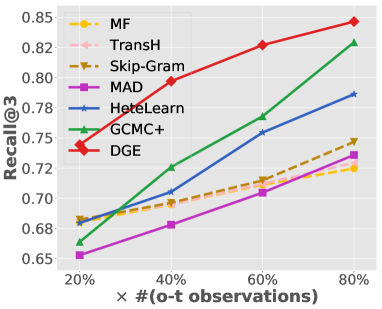
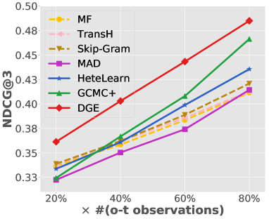
Figure 3: Recall@3 and NDCG@3 on Movie-1m with the sparsity level of object-tag observations varying. Methods denoted by dash lines only consider the first-order proximity, while those with solid lines leverage the high-order relationships in the KG.

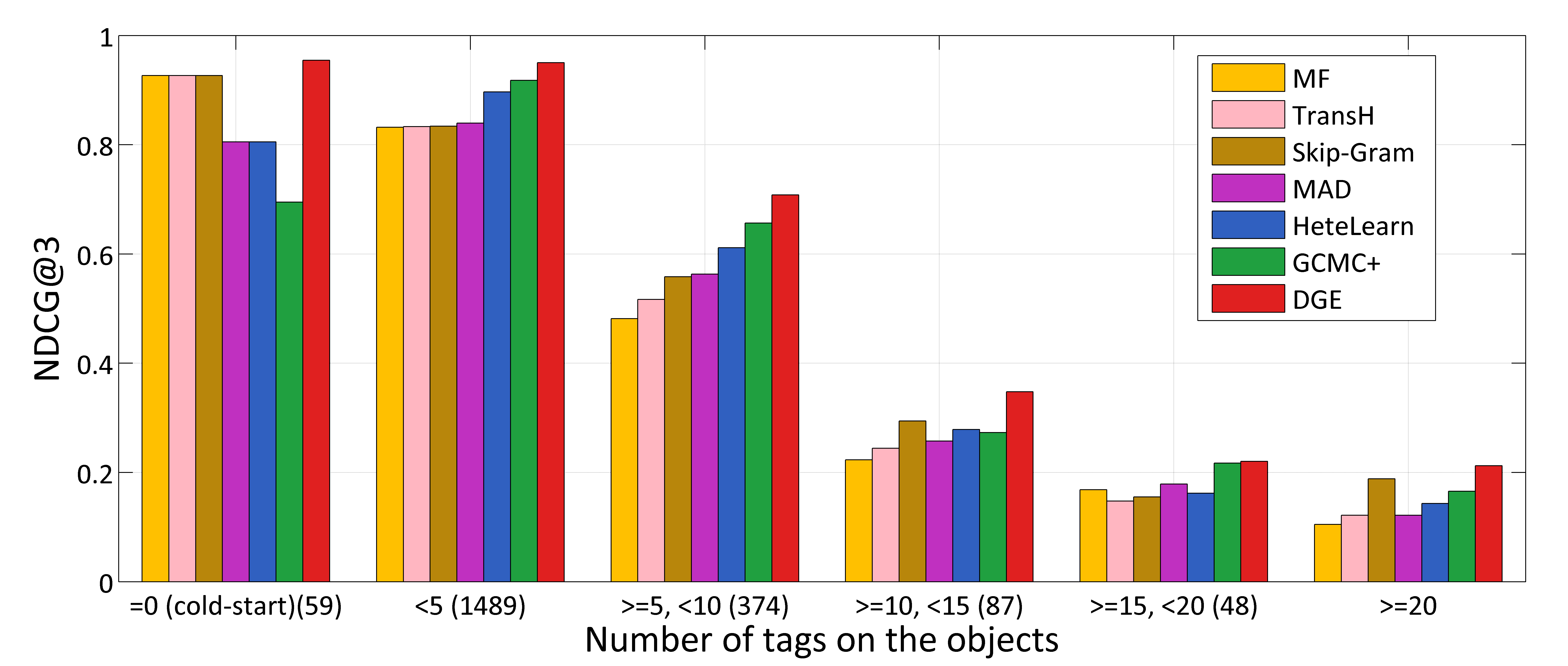
Figure 4: Recall@3 on Movielen-1m of the objects which have different number of tags, and each number in () is the number of test objects satisfying the corresponding condition.

TABLE IV: Top 5 Tags Predicted by Different Methods on Movielens-1M (The movie with * is a cold-start movie.)

Movielens-1M	test truth tags	TransH	Skip-Gram	MAD	HeteLearn	GCMC+	DGE
Billy Madison,	comedy, drama	drama, comedy,	comedy, drama,	thriller, stupid,	drama, comedy,	drama, comedy,	comedy, drama,
(1995)		romance, adventure,	musical, romance,	adam sandler, drama,	action, romance,	war, parody,	horror, crime,
		action	food	comedy	adventure	crime	romance
Sense and Sensibility,	romance, thriller	thriller, comedy,	thriller, teen movie,	drama, based on a book,	thriller, comedy,	romance, thriller,	romance, thriller,
(1995)		adventure, action	romance, John Hughes,	british, hugh grant,	romance, action,	classic, witty,	comedy, classic,
		romance	highschool	romantic	adventure	fantasy	bittersweet
Madonna: Truth or Dare,	documentary,	drama, thriller,	thriller, drama,	thriller, drama,	thriller, drama,	thriller, drama,	drama, thriller,
(1991)*	drama, thriller	comedy, action,	action, comedy,	comedy, action,	comedy, action,	documentary,	documentary,
		romance	adventure	romance	romance	crime, comedy	horror, mystery

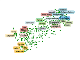
(a) TransH

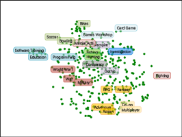
(b) GCMC+

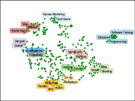
(c) DGE

Figure 5: Visualization of tag embeddings derived by TransH, GCMC+ and DGE on Steam. Tags with the same color are semantically similar. DGE can learn the semantic similarities between tags in the semantic space.

TABLE V: $Recall@k$, $NDCG@k$ on Movielens-1M, LastFM, and Steam based on Different Variants of DGE

Datasets	Methods	Recall@3	NDCG@3	Recall@5	NDCG@5
	SO-GE	0.8101	0.4526	0.8401	0.3343
Movielens-1M	ST-GE	0.7443	0.4207	0.7823	0.3136
	DGE	0.8464	0.4850	0.8677	0.3565
	SO-GE	0.0830	0.0580	0.1211	0.0540
LastFM	ST-GE	0.1928	0.1717	0.2496	0.1444
	DGE	0.2494	0.2129	0.3154	0.1772
	SO-GE	0.3251	0.2425	0.4587	0.2152
Steam	ST-GE	0.2856	0.1977	0.4132	0.1821
	DGE	0.4139	0.3226	0.5100	0.2658

V-D Overall Comparison

The overall performance results on the three datasets are summarized in Table III, and we have following observations:

• DGE beats all other models on the three datasets, especially when predicting the top-3 most relevant tags for objects. The results prove that DGE extracts more essential information from both the first-order and high-order proximities in the KG to predict the missing links more accurately.

• Comparing the methods only modeling the first-order proximity, we find that the Skip-Gram model outperforms MF and three translational distance models on all the datasets. Since the only difference between MF and Skip-Gram is the loss function, the results demonstrate that the skip-gram objective can measure the first-order proximity more accurately than the MSE loss used in MF and the margin loss used in translational distance models.

• Compared with the methods that modeling the high-order relationship in the KG, DGE provides the most relevant tags for objects. It is because that the dual graph encoder in DGE can extract more collaborative information from the high-order proximities while the other methods are affected by some noisy information when conducting random walk or feature aggregation on the input KG.

• DGE outperforms the Skip-Gram model. Both models adopt the skip-gram objective to learn the first-order proximity while DGE captures the high-order proximities simultaneously. The results show that the high-order proximities contain essential information for this task.

V-E Performance on Different Sparsity Levels

To evaluate the robustness of our model given the sparse object-tag observations, we randomly draw samples (20%, 40%, 60%, 80%) of all the observed object-tag pairs for training and compare the results in Fig. 3. Experiments on all the datasets show similar results, thus we only show the results on Movielens-1M.

We find that even with a lack of tagging data, our model predicts more relevant tags than other methods. Considering that the skip-gram objective brings trivial gain in very sparse cases, DGE can still extracts supplementary information from the high-order proximities for better prediction. Moreover, the results of MAD, HeteLearn, GCMC, and our model demonstrate that the dual graph encoder can represent both the object-object and tag-tag relations better in the sparse cases.

V-F Object Cold-Start and Data Sparsity Problems

Fig. 4 shows the performances on those objects which have different numbers of tags in the training set. The first group of bars corresponds to the cold-start examples. These bars show that for cold-start objects, DGE predicts the tags more accurately with the Recall@3 over 0.95, which verify that the high-order proximities enrich the representations of cold-start objects via the dual graph encoder. The baseline methods incorporating high-order relationships underperform the other methods in this case because that the learned models tend to accurately predict the tags for the objects in densely distributed regions (e.g. objects having $>0,<10$ tags in the training set).

Besides, by investigating the performances in the other five groups of bars in Fig. 4, we find that DGE always predicts the most relevant tags compared to other methods. The results illustrate that DGE can mine valuable information from both the first-order and high-order proximities in the KG under different sparse cases.

V-G Ablation Study

To evaluate whether the two GCN encoders in the DGE extract the high-order proximities effectively for link prediction, we replace an encoder of them with a trivial MLP. With this operation, we derive two variants of DGE :

• SO-GE: It only retains the object graph in DGE and replaces the tag GCN encoder with MLP. This model cannot extract the high-order proximity between tags.

• ST-GE: It only retains the tag graph in DGE and a MLP for objects is applied to derive object embeddings containing no the high-order proximity information.

We compare the results on three datasets via these variants and DGE in Table. V. The results prove that the designed dual graph encoder can learn the helpful structural information in the high-order object-object and tag-tag proximities to enhance the prediction performances.

V-H Visualization

We first apply TSNE to the high-dimension tag embeddings derived by TransH, GCMC+ and DGE. The visualization results are shown in Fig. 5. Compared to TransH and GCMC+, tag embeddings derived by DGE can represent the semantic similarities between tags more clearly, which improves the interpretability of the prediction results. For example, the semantically similar tags “Vampire” and “Gothic” are close in Fig. 5 (c) but far apart in Fig. 5 (a) and (b). Besides, DGE clusters tags into multiple classes in the semantic space more explicitly than the other two methods. The results prove that our model can learn the semantic similarities between tags via embedding the high-order proximity between tags explicitly. Accordingly, our model will predict tags that are more probable to be semantically relevant to the target object.

In addition, we give three tagging examples on Movielens-1M in Table IV. We find that for the cold-start movie “Madonna: Truth or Dare, (1991)”, the former four methods provide two most popular tags “drama” and “thriller” without representing the object-object proximity sufficiently, while DGE predicts the accurate tags. This result shows that our model can alleviate the object cold-start problem. For the movie “Sense and Sensibility, (1995)”, the Skip-Gram model predicts the tags more accurately than TransH, proving that the skip-gram objective can better learn the first-order object-tag proximity. Besides, for the latter two movies, our model puts the most relevant tags at the top of the lists, which further proves the prediction accuracy of DGE.

VI Conclusions

In this paper, we propose a Dual Graph Embedding (DGE) method in an auto-encoding architecture to capture the first-order and high-order proximities in the input KG for the object-tag link prediction task. Here the dual graphs include the object and tag graphs that are built to depict the high-order proximities. Then the encoder embeds the two types of high-order proximities in the dual graphs into object and tag embeddings. The decoder models the first-order proximity between objects and tags over the global proximity structure from the skip-gram perspective. Under the supervision of the decoder, the similarity information from both the first-order and high-order proximities is extracted for better prediction.

References

- [1] X. Wang, X. He, Y. Cao, M. Liu, and T.-S. Chua, “Kgat: Knowledge graph attention network for recommendation,” in Proceedings of the 25th ACM SIGKDD International Conference on Knowledge Discovery & Data Mining. ACM, 2019, p. 950–958.
- [2] F. M. Belém, J. M. Almeida, and M. A. Gonçalves, “A survey on tag recommendation methods,” J. Assoc. Inf. Sci. Technol., vol. 68, no. 4, p. 830–844, Apr. 2017.
- [3] K. H. L. Tso-Sutter, L. B. Marinho, and L. Schmidt-Thieme, “Tag-aware recommender systems by fusion of collaborative filtering algorithms,” in Proceedings of the 2008 ACM Symposium on Applied Computing. ACM, 2008, p. 1995–1999.
- [4] A. Bordes, N. Usunier, A. Garcia-Duran, J. Weston, and O. Yakhnenko, “Translating embeddings for modeling multi-relational data,” in Advances in Neural Information Processing Systems 26. Curran Associates, Inc., 2013, pp. 2787–2795.
- [5] Z. Wang, J. Zhang, J. Feng, and Z. Chen, “Knowledge graph embedding by translating on hyperplanes,” AAAI Conference on Artificial Intelligence, 2014.
- [6] Y. Lin, Z. Liu, M. Sun, Y. Liu, and X. Zhu, “Learning entity and relation embeddings for knowledge graph completion,” AAAI Conference on Artificial Intelligence, 2015.
- [7] S. Ji, S. Pan, E. Cambria, P. Marttinen, and P. S. Yu, “A survey on knowledge graphs: Representation, acquisition and applications,” ArXiv, vol. abs/2002.00388, 2020.
- [8] Z. Jiang, H. Liu, B. Fu, Z. Wu, and T. Zhang, “Recommendation in heterogeneous information networks based on generalized random walk model and bayesian personalized ranking,” in Proceedings of the Eleventh ACM International Conference on Web Search and Data Mining. ACM, 2018, p. 288–296.
- [9] R. van den Berg, T. N. Kipf, and M. Welling, “Graph convolutional matrix completion,” KDD, 2017.
- [10] X. Wang, X. He, M. Wang, F. Feng, and T.-S. Chua, “Neural graph collaborative filtering,” in Proceedings of the 42nd International ACM SIGIR Conference on Research and Development in Information Retrieval. ACM, 2019, p. 165–174.
- [11] Q. Wang, Z. Mao, B. Wang, and L. Guo, “Knowledge graph embedding: A survey of approaches and applications,” IEEE Transactions on Knowledge and Data Engineering, vol. 29, no. 12, pp. 2724–2743, 2017.
- [12] G. Ji, S. He, L. Xu, K. Liu, and J. Zhao, “Knowledge graph embedding via dynamic mapping matrix,” in Proceedings of the 53rd Annual Meeting of the Association for Computational Linguistics and the 7th International Joint Conference on Natural Language Processing (Volume 1: Long Papers). ACL, Jul. 2015, pp. 687–696.
- [13] S. He, K. Liu, G. Ji, and J. Zhao, “Learning to represent knowledge graphs with gaussian embedding,” in Proceedings of the 24th ACM International on Conference on Information and Knowledge Management. ACM, 2015, p. 623–632.
- [14] H. Xiao, M. Huang, and X. Zhu, “TransG : A generative model for knowledge graph embedding,” in Proceedings of the 54th Annual Meeting of the Association for Computational Linguistics (Volume 1: Long Papers). ACL, Aug. 2016, pp. 2316–2325.
- [15] S. Rendle and L. Schmidt-Thieme, “Pairwise interaction tensor factorization for personalized tag recommendation,” in Proceedings of the Third ACM International Conference on Web Search and Data Mining. ACM, 2010, p. 81–90.
- [16] A. Rae, B. Sigurbjörnsson, and R. van Zwol, “Improving tag recommendation using social networks,” in Adaptivity, Personalization and Fusion of Heterogeneous Information, 2010.
- [17] D. Liang, J. Altosaar, L. Charlin, and D. M. Blei, “Factorization meets the item embedding: Regularizing matrix factorization with item co-occurrence,” in Proceedings of the 10th ACM Conference on Recommender Systems. ACM, 2016, p. 59–66.
- [18] T. Mikolov, I. Sutskever, K. Chen, G. Corrado, and J. Dean, “Distributed representations of words and phrases and their compositionality,” in Proceedings of the 26th International Conference on Neural Information Processing Systems - Volume 2. Curran Associates Inc., 2013, p. 3111–3119.
- [19] O. Levy and Y. Goldberg, “Neural word embedding as implicit matrix factorization,” in Proceedings of the 27th International Conference on Neural Information Processing Systems - Volume 2. MIT Press, 2014, p. 2177–2185.
- [20] T. N. Kipf and M. Welling, “Semi-supervised classification with graph convolutional networks,” in International Conference on Learning Representations (ICLR), 2017.
- [21] A. Mnih and K. Kavukcuoglu, “Learning word embeddings efficiently with noise-contrastive estimation,” in Proceedings of the 26th International Conference on Neural Information Processing Systems - Volume 2. Curran Associates Inc., 2013, p. 2265–2273.
- [22] Y. Koren, R. Bell, and C. Volinsky, “Matrix factorization techniques for recommender systems,” Computer, vol. 42, no. 8, pp. 30–37, 2009.
- [23] Y. Cao, X. Wang, X. He, Z. Hu, and T.-S. Chua, “Unifying knowledge graph learning and recommendation: Towards a better understanding of user preferences,” in World Wide Web. ACM, 2019, p. 151–161.
- [24] P. P. Talukdar and K. Crammer, “New regularized algorithms for transductive learning,” in Proceedings of the 2009th European Conference on Machine Learning and Knowledge Discovery in Databases - Volume Part II. Springer-Verlag, 2009, p. 442–457.
- [25] Z. Zhang, Y. Liu, Z. Zhang, and B. Shen, “Fused matrix factorization with multi-tag, social and geographical influences for poi recommendation,” World Wide Web, vol. 22, no. 3, p. 1135–1150, 2019.