An ergodic-averaging method to differentiate covariant Lyapunov vectors

Abstract

Covariant Lyapunov vectors or CLVs span the expanding and contracting directions of perturbations along trajectories in a chaotic dynamical system. Due to efficient algorithms to compute them that only utilize trajectory information, they have been widely applied across scientific disciplines, principally for sensitivity analysis and predictions under uncertainty. In this paper, we develop a numerical method to compute the directional derivatives of the first CLV along its own direction; the norm of this derivative is also the curvature of one-dimensional unstable manifolds. Similar to the computation of CLVs, the present method for their derivatives is iterative and analogously uses the second-order derivative of the chaotic map along trajectories, in addition to the Jacobian. We validate the new method on a super-contracting Smale-Williams Solenoid attractor. We also demonstrate the algorithm on several other examples including smoothly perturbed Arnold Cat maps, and the Lorenz’63 attractor, obtaining visualizations of the curvature of each attractor. Furthermore, we reveal a fundamental connection of the derivation of the CLV self-derivative computation with an efficient computation of linear response of chaotic systems.

1 Introduction

Linear response refers to the linear change in the long-term or statistical behavior of a dynamical system, as a result of a small parameter perturbation. In chaotic systems, a linear response formula was developed by Ruelle ruelle ruelle1 , which is rigorously proved for uniformly hyperbolic systems, the simplest setting in which a chaotic attractor can occur. Linear response has been observed in practical chaotic systems wherein dissipative dynamics dominate wormell angxiu-jfm patrick-fluid-1 nisha-shadowing francisco . A unique ergodic stationary physical probability distribution, known as an SRB measure srb , is achieved on uniformly hyperbolic attractors. Linear response gives us a quantitative estimate of the derivative of the SRB measure with respect to system parameters, using information only from the unperturbed system.

This statistical derivative can enable typical applications of sensitivity analysis, such as uncertainty quantification, design, optimization and control problems in chaotic systems. These applications are currently limited in chaotic systems because the computation of linear response, through Ruelle’s theoretical formula, remains a challenging problem. Some new numerical methods are being actively developed as of this writing (nisha-s3 angxiu ) in which Ruelle’s formula is transformed into a well-conditioned ergodic-averaging computation; other promising methods include shadowing-based methods qiqi-shadowing angxiu-nilss , and approximate evaluations of Ruelle’s response using fluctuation-dissipation theorems extended to SRB-type measures majda1 lucarini-linear-response majda .

In this work, we develop a numerical method for derivatives on the unstable manifold of certain quantities fundamental to linear response. These derivatives are needed for an efficient computation of a regularized version of Ruelle’s formula. Focusing on one-dimensional unstable manifolds, the proposed numerical method gives the derivative of the unstable Covariant Lyapunov Vector (CLV) kuptsov along its own direction. As a byproduct, we obtain the unstable derivative of the local expansion factor of the unstable CLV, and this quantity appears in the computation of linear response.

We expect the CLV self-derivatives computed in this paper, which describe the curvature of the attractor manifold, to be applicable beyond linear response. CLVs are specific bases for tangent spaces along a trajectory, characterized by Lyapunov exponents. Ginelli et al.’s ginelli efficient algorithm to compute CLVs has led to several applications of Lyapunov analysis in engineering, in both deterministic and stochastic chaotic systems. These applications include uncertainty quantification, data assimilation and forecasting, across a range of disciplines such as numerical weather prediction and aerospace engineering (beeson , angxiu-jfm , lucarini_climate , francisco ; see ginelli-clv-review for a survey of applications of Lyapunov analysis).

The numerical method we develop in this work for the directional derivatives of CLVs in their respective directions is henceforth known as the differential CLV method. We shall refer to these derivatives as CLV self-derivatives. In the case of a one-dimensional unstable manifold, the CLV corresponding to the largest Lyapunov exponent is the unit tangent vector field along the unstable manifold. The norm of this CLV self-derivative is hence also the curvature of the unstable manifold.

The connection we reveal with linear response is via a byproduct of the differential CLV method: the unstable derivative of the local expansion factors of the unstable CLVs. This derivative is a key ingredient in an iterative computation of a fundamental quantity intimately connected to linear response. This quantity, which we refer to as the logarithmic density gradient, indicates how the SRB measure changes along unstable manifolds in the attractor. More precisely, in the case of one-dimensional unstable manifolds, which is the focus of this paper, this quantity is the unstable derivative of the logarithm of the SRB density on the unstable manifold. This connection shows one potential application of the recursive method developed in this paper: the computation of linear response in chaotic systems.

The outline of the subsequent sections is as follows. In section 2, we briefly summarize the theory of CLVs and establish the setting we derive our results in: uniformly hyperbolic attractors. The differential CLV method is derived in section 3; while the main steps are in section 3.3, notational setup and the intuition for the steps are developed in the prior subsections. We validate the method using a super-contracting Solenoid map in section 4.1. Further numerical experiments demonstrating the method on the Lorenz’63 attractor, a volume-preserving perturbed Cat map, a dissipative perturbed Cat map, and the Hénon map are in sections 4.2, 4.3, 4.4 and 4.5 respectively. The implication of the method for the computation of linear response is discussed in section 5. We summarize our results and conclude in section 6.

2 Problem setup, definitions and review of Covariant Lyapunov Vectors

The dynamical system studied in this paper is the iterative application of a smooth ($C^{3}$) self-map $\varphi:\mathbb{M}\to\mathbb{M}$ of a domain $\mathbb{M}$, which is a compact subset of $\mathbb{R}^{m}$. We write $\varphi^{n}$ to denote an $n$-time composition of $\varphi$; that is, $\varphi^{n}=\varphi\circ\varphi^{n-1}$, $n\in\mathbb{Z}^{+}$, where $\varphi^{0}$ is the identity function on $\mathbb{R}^{m}$. The iterates under $\varphi$, or the points along orbits of the dynamical system, are represented using the following subscript notation: if $x\in\mathbb{M}$, $x_{n}:=\varphi^{n}x$; $x_{0}$ is simply written as $x$, which we use to denote an arbitrary phase point. A similar notation is also adopted for scalar or vector-valued functions or observables. If $f$ is an observable, $f_{n}:=f\circ\varphi^{n}.$ The derivative with respect to the state is denoted as $d$ and the partial derivative operators, with respect to the Euclidean coordinate functions $x_{1},x_{2},\cdots,x_{m}$ are written as $\partial_{1},\partial_{2},\cdots,\partial_{m},$ respectively. For instance, if $f:\mathbb{M}\to\mathbb{R}$ is a scalar-valued observable, the derivative $df$ evaluated at $x$ is given by $df(x)=[\partial_{1}f(x),\cdots,\partial_{m}f(x)]^{T}.$ Using the notation introduced, an application of the chain rule would be as follows:

$$(df_{n})^{T}=((df)_{n})^{T}\;d\varphi^{n}.$$

Finally, we assume the existence of an ergodic, physical, invariant measure for $\varphi$, known as the SRB measure and denoted $\mu$. As a result, ergodic (Birkhoff) averages of observables in $L^{1}(\mu)$ converge to their expectations with respect to $\mu$: $\lim_{N\to\infty}(1/N)\sum_{n=0}^{N-1}f_{n}(x)=\langle f,\mu\rangle$ for Lebesgue-a.e. $x\in\mathbb{M}.$ Note that such a measure is guaranteed to exist srb in the uniformly hyperbolic setting, which we discuss in section 2.2.

2.1 Tangent dynamics

In order to introduce covariant Lyapunov vectors (CLVs), whose derivatives are the subject of this paper, we briefly discuss the asymptotic behavior of tangent dynamics in chaotic systems. We refer to as tangent dynamics the linear evolution of perturbations under the Jacobian matrix, $d\varphi$. The Jacobian matrix evaluated at an $x\in\mathbb{M}$ is denoted $d\varphi_{x}$. Denoting the tangent space at $x$ as $T_{x}\mathbb{M}$, $d\varphi^{n}_{x}$ is a map from $T_{x}\mathbb{M}$ to $T_{x_{n}}\mathbb{M}$. Given a tangent vector $v_{0}\in T_{x}\mathbb{M}$, we denote its iterate under the tangent dynamics at time $n$ as $v_{n}\in T_{x_{n}}\mathbb{M}.$ That is, $v_{n}=d\varphi^{n}_{x}v_{0}.$ Intuitively, if a perturbation of norm ${\cal O}(\epsilon)$ is applied at $x$ along $v_{0}$, up to first order in $\epsilon$, the deviation from the original orbit starting at $x$, after time $n$, is along $v_{n}$. In other words,

$$v_{n}=\lim_{\epsilon\to 0}\dfrac{\varphi^{n}(x+\epsilon v_{0})-x_{n}}{\epsilon}=d\varphi^{n}_{x}v_{0}.$$ (1)

In practice, the above equation for the tangent dynamics is solved iteratively, along a reference orbit $\left\{x_{n}\right\}$, since using the chain rule, $d\varphi^{n}_{x}=d\varphi_{x_{n-1}}\cdots d\varphi_{x},$ and hence $v_{n+1}=d\varphi_{x_{n}}v_{n}.$ A classical result in nonlinear dynamics, known as the Oseledets multiplicative ergodic theorem (OMET) arnold deals with the asymptotic behavior of $v_{n}$ as $n\to\infty$, in ergodic systems. The OMET implies the following: at $\mu$-a.e. $x\in\mathbb{M}$, the tangent space splits as a direct sum, $T_{x}\mathbb{M}=\oplus_{i=1}^{p}E^{i}_{x}$, $p\leq m$, where $E^{i}_{x}$ are $d\varphi$-invariant subspaces in the sense that $d\varphi_{x}E^{i}_{x}=E^{i}_{\varphi x}$. This splitting is based on the asymptotic, exponential growth/decay rates of tangent dynamics in the subspaces $E^{i}_{x}$. More precisely, for $\mu$-a.e. $x\in\mathbb{M}$, if $v^{i}_{0}\in E^{i}_{x}$, its norm under the tangent dynamics grows/decays exponentially at a rate that converges to a constant. The limits

$$\lambda_{x,i}:=\lim_{n\to\infty}\dfrac{1}{n}\log\left(\dfrac{\left\lVert v^{i}_{n}\right\rVert}{\left\lVert v^{i}_{0}\right\rVert}\right),$$ (2)

$1\leq i\leq p$, are known as the Lyapunov exponents (LEs). Since $\varphi$ is an ergodic map with respect to $\mu$, the LEs are constants independent of $x$, for $\mu$-a.e. $x$; we denote the LEs $\lambda_{i}$, in descending order as $\lambda_{1}\geq\lambda_{2}\geq\cdots\geq\lambda_{p}.$ In our setting, $\varphi$ is a chaotic map, which means that $\lambda_{1}>0$. Let $d_{u}$ be the number of positive LEs, and $d_{s}=p-d_{u}$ be the number of negative LEs. Then, $E^{u}_{x}:=\oplus_{i=1}^{d_{u}}E^{i}_{x}$ is called the unstable subspace of $T_{x}\mathbb{M}.$ In other words, the unstable subspace $E^{u}_{x}$ is the set of tangent vectors that asymptotically decay exponentially in norm under tangent dynamics backward in time; by definition, the unstable subspaces at points on a chaotic orbit are non-empty. This sensitivity to perturbations is the so-called butterfly effect that defines chaotic systems.

Similarly, the set of tangent vectors that asymptotically decay exponentially in norm under the tangent dynamics, make up the stable subspace, denoted $E^{s}_{x}:=\oplus_{i=d_{u}+1}^{p}E^{i}_{x}=T_{x}\mathbb{M}\backslash E^{u}_{x}$. If each $E^{i}$ is one-dimensional and $p=m$, the covariant Lyapunov vectors or CLVs, denoted as $V^{i}$ in this paper, are unit vector fields along $E^{i}.$ That is, CLVs satisfy the following properties at $\mu$-a.e. $x$:

• The covariance property:

  $$d\varphi_{x}V^{i}_{x}\in E^{i}_{x_{1}}.$$ (3)

  Since by definition $V^{i}_{x}$ is a unit vector, we introduce a scalar function $z_{\cdot,i}:\mathbb{M}\to\mathbb{R}^{+}$ defined as $z_{x,i}:=\left\lVert d\varphi_{x}V^{i}_{x}\right\rVert,$ to indicate the local stretching or contraction factor of the $i$th CLV. Hence, the covariance property of the $i$th CLV can be expressed as

  $$d\varphi_{x}V_{x,i}=z_{x,i}V^{i}_{x_{1}}.$$ (4)

• The $i$th CLV grows/decays asymptotically on an exponential scale, at the rate $\lambda_{i}$, and, in addition, is invariant under time-reversal:

  $$\lambda_{i}:=\lim_{n\to\pm\infty}\frac{1}{n}\log\left\lVert d\varphi^{n}_{x}V^{i}_{x}\right\rVert.$$ (5)

2.2 Uniform hyperbolicity

We consider an idealized class of chaotic systems known as uniformly hyperbolic systems, which are characterized by uniform expansions and contractions of tangent vectors. In uniformly hyperbolic systems, there exist constants $c>0$ and $\lambda\in(0,1)$ such that, at every point $x\in\mathbb{M}$, i) every stable tangent vector $v\in E^{s}_{x}$ satisfies: $\left\lVert d\varphi^{n}_{x}v\right\rVert\leq c\;\lambda^{n}\left\lVert v\right\rVert$, and ii) every unstable tangent vector $v\in E^{u}_{x}$ satisfies: $\left\lVert d\varphi^{-n}_{x}v\right\rVert\leq c\;\lambda^{n}\left\lVert v\right\rVert$, for all $n\in\mathbb{N}$. As a result, in these systems, there exists an upper (lower) bound that is independent of the base point $x$, on the slowest contracting (stretching) factors among $z_{x,i}$. In particular, defining $C:=c\lambda$, we have $z_{x,i}\geq(1/C)$, $1\leq i\leq d_{u}$ and $z_{x,i}\leq C$, $d_{u}+1\leq i\leq d.$ From the definition of the LEs (Eq. 5), it is also clear that they are the ergodic (Birkhoff) averages of the stretching/contraction factors:

$$\langle\log z_{\cdot,i},\mu\rangle:=\lim_{N\to\infty}\frac{1}{N}\sum_{n=0}^{N-1}\log{z_{x_{n},i}}=\lambda_{i},\;\;x\in\mathbb{M}\;\;\mu-{\rm a.e}.$$ (6)

2.3 Examples

A simple example of a uniformly hyperbolic system is Arnold’s Cat map, a smooth self-map of the surface of the torus ($\mathbb{T}^{2}\equiv\mathbb{R}^{2}/\mathbb{Z}^{2}$):

$$\varphi([{\rm x}_{1},{\rm x}_{2}]^{T})=\begin{bmatrix}2&1\\ 1&1\end{bmatrix}\begin{bmatrix}{\rm x}_{1}\\ {\rm x}_{2}\end{bmatrix}\;{\rm mod}\;1.$$ (7)

This is a linear hyperbolic system, i.e., the Jacobian matrix of the map is a constant in phase space and has eigenvalues other than 1. In this simple example, the CLVs and the stretching/contracting factors, are also independent of the phase point. The logarithm of the eigenvalues of the constant Jacobian matrix, are the LEs of this map: $\lambda_{1}=\log|(3+\sqrt{5})/2|$ and $\lambda_{2}=\log|(3-\sqrt{5})/2|.$ It is also clear that $E^{1}=E^{u}$ and $E^{2}=E^{s}$ are one-dimensional subspaces spanned by $V^{1}$ and $V^{2}$, the eigenvectors of the Jacobian matrix at eigenvalues of $e^{\lambda_{1}}$ and $e^{\lambda_{2}}$ respectively. Moreover, $z_{1}$ and $z_{2}$ are also constant on $\mathbb{R}^{2}/\mathbb{Z}^{2}$: $z_{1}=e^{\lambda_{1}}$, and $z_{2}=e^{\lambda_{2}}$. Further, the SRB measure for this map is the Lebesgue measure on $\mathbb{R}^{2}/\mathbb{Z}^{2}.$

Since the Jacobian matrix is symmetric, the CLVs $V^{1}$ and $V^{2}$ are everywhere orthogonal to each other, but it is worth noting that this is a special case. In a generic uniformly hyperbolic system, it is only true that the angle between the CLVs is uniformly bounded away from zero. The perturbed Cat maps treated later have additive perturbations to the Cat map above that are smooth functions on the torus. Two types of smooth perturbations are considered later, both designed to produce non-uniform behavior of the CLVs. Both perturbed Cat maps are still uniformly hyperbolic, and differ in whether or not the resulting maps are area-preserving, in order to represent the two distinct cases of conservative (symplectic) and dissipative chaos.

2.4 Lack of differentiability of $E^{u}$ and $E^{s}$

On hyperbolic sets, it is known that $E^{u}$ and $E^{s}$ are Hölder-continuous functions of phase space, in a sense clarified in Appendix section A. When the Hölder exponent $\beta$, from Appendix section A, equals 1, we have Lipschitz continuity, but this is indeed rare. Several examples (see hasselblatt_prevalence_1999 and references therein) have been constructed in which $\beta$ is made to be arbitrarily small at almost all phase points, even in $C^{\infty}$ maps. In rare cases, $E^{u}$ and $E^{s}$ are continuously differentiable when a certain bunching condition (hasselblatt_prevalence_1999 , or section 19.1 of katok ) is satisfied by the LEs.

Revisiting the examples, the perturbed Cat maps discussed above belong to the rare category of maps with continuously differentiable stable/unstable subspaces. In fact, it can be shown that all uniformly hyperbolic maps on compact sets of dimension 2 belong to this category (see Corollary 19.1.11 of katok ). While it would be typical of a higher-dimensional map, even when uniformly hyperbolic, to show non-smoothness of the stable and unstable subspaces, we have chosen to work with two-dimensional examples in this paper for easy visualization of the subspaces, which are lines in these maps.

2.5 Derivatives of CLVs in their own directions

While the CLVs may lack differentiability on $\mathbb{M}$, they have directional derivatives in their own directions. In fact, it can be shown that these directional derivatives, which we refer to here as CLV self-derivatives, are themselves Hölder continuous with the same exponent $\beta$ (see Remark in the proof of Theorem 19.1.6 of katok ). To wit, in two-dimensional uniformly hyperbolic systems, examples of which are considered in this paper, both partial derivatives (along coordinate directions) of the CLVs exist, and hence the CLVs have directional derivatives in all directions. The purpose of this paper, however, is to numerically compute directional derivatives of CLVs along their respective directions in a general uniformly hyperbolic system, regardless of their differentiability in phase space. Thus, we compute the CLV self-derivatives, without using the partial derivatives along coordinate directions, which may not exist. The CLV self-derivatives are denoted by $W^{i}_{x}\in T_{x}T_{x}\mathbb{M}\equiv\mathbb{R}^{m}$. They are defined using curves ${\mathcal{C}}_{x,i}:[-\epsilon_{x},\epsilon_{x}]\to\mathbb{M}$ with the properties: i) ${\mathcal{C}}_{x,i}(0)=x$, ii) ${\mathcal{C}}_{x,i}^{\prime}(t)=V^{i}({\mathcal{C}}_{x,i}(t)),\;\forall\;t\in[-\epsilon_{x},\epsilon_{x}]$, as

$$W^{i}_{x}:=\lim_{t\to 0}\dfrac{V^{i}_{{\mathcal{C}}_{x,i}(t)}-V^{i}_{x}}{t}.$$ (8)

For example, in the case of a 1-dimensional unstable manifold, the curve ${\mathcal{C}}_{x,1}$, coincides with a local unstable manifold at $x.$ Further discussion on the definition of $W^{i}$ based on these curves, is postponed until section 3.1. Here we explain the existence of these curves. The vector fields $V^{i}$, $1\leq i\leq d_{u}$ are infinitely smooth on an open set in a local unstable manifold, and likewise, $V^{i}$, for $d_{u}+1\leq i\leq d$ are infinitely smooth on an open set in a local stable manifold. As a result, due to the existence and uniqueness theorem, the flow of vector field $V^{i}$, denoted by the curve ${\mathcal{C}}_{\cdot,i}$ exists and is uniquely defined, for some $\epsilon_{\cdot}>0,$ justifying the definition in Eq. 8.

Given $T_{x}\mathbb{M},T_{x}T_{x}\mathbb{M}\equiv\mathbb{R}^{m}$, we write all vectors in these spaces in Euclidean coordinates. The output of the numerical method to be developed, $W^{i}$, are $d$-dimensional vector fields consisting of component-wise directional derivatives of $V^{i}.$

2.6 Computations along trajectories

Before we delve into the differential CLV method, we note that $W^{i}$, being self-derivatives of CLVs, are naturally defined along trajectories, just like the CLVs. Thus, we seek a trajectory-based iterative procedure to compute them. We assume as input to the method the map, its Jacobian and second-order derivative, all computed along a long, $\mu$-typical trajectory. The CLVs that need to be differentiated are also assumed as input, along the trajectory. To compute the CLVs, a standard algorithm such as Ginelli et al.’s algorithm ginelli can be used. This is an iterative procedure involving repeated QR factorizations of nearby subspaces to the one that is spanned by the required CLVs. For Ginelli et al.’s algorithm, the reader is referred to ginelli and florian for its convergence with respect to trajectory length; for other algorithms that involve LU factorizations instead of QR, we refer to kuptsov .

Besides using the computed CLVs as input, the differential CLV method we develop here for $W^{i}$ does not follow Ginelli et al.’s or other algorithms for the computation of CLVs, primarily because the vector fields $W^{i}$ do not satisfy the covariance property. But the method resembles the latter algorithms in being iterative and trajectory-based. One advantage of trajectory-based computation is that we exploit for fast convergence (this aspect again being similar to the CLV computation algorithms) the hyperbolic splitting of the tangent space. This will be clear at the end of the next section in which we give a step-by-step derivation.

3 An algorithm to compute the directional derivatives of CLVs in their own directions

In this section, we derive a numerical method to determine the quantity of interest, $W^{i},$ which is defined in Eq. 8. In particular, fixing a reference trajectory $x,x_{1},\cdots,$ we develop an iterative scheme that converges asymptotically to vectors $W^{i}_{n}:=W^{i}_{x_{n}}$, under certain conditions (Appendix C), starting from an arbitrary guess for $W^{i}_{0}:=W^{i}_{x}\in\mathbb{R}^{m}.$ The derivation results in the following iteration, valid for $1\leq i\leq d_{u},n\in\mathbb{Z}^{+}$, and guaranteed to converge when $i=1$:

$$W^{i}_{n+1}=\Big{(}I-V^{i}_{n+1}(V^{i}_{n+1})^{T}\Big{)}\dfrac{d^{2}\varphi(x_{n}):V^{i}_{n}\>V^{i}_{n}+d\varphi(x_{n})W^{i}_{n}}{z_{n,i}^{2}}.$$ (9)

The iteration mainly uses the chain rule and the covariance property of $V^{i}$, in a convenient set of coordinate systems centered along each $\mu$-typical trajectory. These trajectory-based coordinates help us uncover each term on the right hand side of Eq. 9.

3.1 Change of coordinates and associated notation

Fix a $\mu$-typical point $x\in\mathbb{M}$, and consider again the curves ${\mathcal{C}}_{x,i}$, $1\leq i\leq d,$ which were introduced to define $W^{i}$ in Eq. 8. To reiterate, the curves ${\mathcal{C}}_{x,i}:[-\epsilon_{x},\epsilon_{x}]\to\mathbb{M}$ are such that i) ${\mathcal{C}}_{x,i}(0)=x$ and ii) ${\mathcal{C}}_{x,i}^{\prime}(t)=V^{i}({\mathcal{C}}_{x,i}(t)),$ for all $t\in[-\epsilon_{x},\epsilon_{x}].$ There exists a measurable function $x\to\epsilon_{x}$ that defines the extent of the curves so that such a coordinate change, from $[-\epsilon_{x},\epsilon_{x}]^{m}$ to a neighborhood of $x$, exists and is additionally differentiable. This follows from an assertion proved in standard stable-unstable manifold theory: a closed $\epsilon_{x}$ Euclidean ball around the origin in $\mathbb{R}^{d_{u}}$ ($\mathbb{R}^{d_{s}}$) has an embedding into a local unstable (stable) manifold at $x$. These pointwise coordinate systems are referred to as Lyapunov charts or adapted coordinates in the theoretical literature (katok Ch. 6, ledrappier-young ).

In writing Eq. 8, we made a particular choice of adapted coordinates. We chose coordinate functions that are adapted specifically to the CLVs, as opposed to any other basis of $T_{x}\mathbb{M}$, in the following sense. At each $x$, the image of the $i$th Euclidean basis vector $e_{i}$, under the differential of the coordinate change, is $V^{i}$. More intuitively, we have chosen adapted coordinates such that the $i$th Euclidean coordinate axis corresponds, under these coordinate changes, to points that are perturbations along $V^{i}$. Thus, our quantity of interest, can be written, by definition of CLV-adapted coordinates, as

$$W^{i}_{x}=\frac{d}{dt}(V^{i}\circ{\mathcal{C}}_{x,i})(0).$$ (10)

3.2 The map in adapted coordinates

Now we introduce the transformation induced by $\varphi:\mathbb{M}\to\mathbb{M}$ on the CLV-adapted coordinates on $\mathbb{R}^{m}$. To do that, we fix an $i\leq d_{u}$ and focus on the relationship between the curves ${\mathcal{C}}_{x_{1},i}:[-\epsilon_{x_{1}},\epsilon_{x_{1}}]\to\mathbb{M}$ and $\varphi\circ{\mathcal{C}}_{x,i}:[-\epsilon_{x},\epsilon_{x}]\to\mathbb{M}.$ Define $f_{x,i}:=({\mathcal{C}}_{x_{1},i})^{-1}\circ\varphi\circ{\mathcal{C}}_{x,i},$ noting that this definition makes sense at a point $t\in[-\epsilon_{x},\epsilon_{x}]$ whenever $\varphi({\mathcal{C}}_{x,i}(t))$ lies in the image of ${\mathcal{C}}_{x_{1},i}.$ The function, $x\to\epsilon_{x}$, which determines the size of the local unstable manifold at each $x$, can be chosen such that orbits of

$$f_{x,i}^{-n}:=f_{x_{n},i}^{-1}\circ\cdots\circ f_{x_{1},i}^{-1}\circ f_{x,i}^{-1},n\in\mathbb{Z}^{+}$$ (11)

are well-defined at almost every $x$, for $1\leq i\leq d_{u},$ within local unstable manifolds centered along the backward $\varphi$-orbit. Clearly, 0 is a fixed point of $f_{x,i}^{n}$ for all $n\in\mathbb{Z}$, and corresponds to the $\varphi$-orbit $\cdots,x_{-1},x,x_{1},x_{2},\cdots,.$ Intuitively, if an orbit of $f_{x,i}$ excluding the fixed point, say $\left\{t_{n}:=f_{x,i}^{n}(t)\right\}$, exists, it means that ${\mathcal{C}}_{x_{n},i}(t_{n})$ lies in sufficiently small local unstable manifolds of $x_{n}$, at each $n.$ The sizes of the local unstable manifolds can be controlled in order for such orbits to be well-defined (in particular, see Lemma 2.2.2 of ledrappier-young ).

To summarize, we make a specific choice of $x\to\epsilon_{x}$ such that the curves ${\mathcal{C}}_{x_{n},i}$ at each $n$ lie inside a local unstable manifold at $x_{n}$, and are tangent to $V^{i}_{n}:=V^{i}_{x_{n}}.$ This allows us to obtain expressions for the derivative of a CLV $V^{i}_{n+1}$ with respect to $V^{i}_{n},$ which will in turn enter into the computation of $W^{i}.$ In particular, using CLV-adapted coordinates, a suitable map $x\to\epsilon_{x}$, as described above, and the definition of $f_{x,i}$,

$$(df_{x,i}/dt)(0)=z_{x,i}.$$ (12)

Now we usefully relate the iterates through $\varphi$ of the differential operator on $\mathbb{M}$ corresponding to the vector field $V^{i}$, and its analog on $\mathbb{R}$: $d/dt$, along the trajectory lying in the unstable manifold of $x_{n}$. In particular, for the function $V^{i}$, when combined with Eq. 10, and Eq. 12,

$$\frac{d\left(V^{i}\circ\varphi\circ{\mathcal{C}}_{x,i}\right)}{dt}(0) =\frac{d\left(V^{i}\circ{\mathcal{C}}_{x_{1},i}\circ f_{x,i}\right)}{dt}(0)$$

$$=z_{x,i}\;W^{i}_{x_{1}}.$$ (13)

3.3 Computation of unstable CLV self-derivatives

Starting from Eq. 13, and by definition of CLVs (Eq. 4)

$$W^{i}_{x_{1}} =\dfrac{1}{z_{x,i}}\dfrac{d}{dt}\left(\frac{d\varphi_{{\mathcal{C}}_{x,i}}\;V^{i}_{{\mathcal{C}}_{x,i}}}{z_{{\mathcal{C}}_{x,i},i}}\right)(0)$$ (14)

$$=\dfrac{1}{z_{x,i}^{2}}\dfrac{d}{dt}\left(d\varphi_{{\mathcal{C}}_{x,i}}\right)(0)\;V^{i}_{x}+\dfrac{1}{z_{x,i}^{2}}d\varphi_{x}\;\dfrac{d}{dt}(V^{i}_{{\mathcal{C}}_{x,i}})(0)$$

$$+V^{i}_{x_{1}}\;\dfrac{d}{dt}\left(\dfrac{1}{z_{{\mathcal{C}}_{x,i},i}}\right)(0)$$ (15)

By Eq. 10, we can write the second term above as $(1/z_{x,i})^{2}\>d\varphi_{x}\>W^{i}_{x}.$ The first term can be written using the chain rule in terms of the $m\times m\times m$ second-order derivative of $\varphi$, which is a bilinear form denoted as $d^{2}\varphi.$ Let the elements of the second-order derivative of the map be indexed such that $d^{2}\varphi[i,j,k]=\partial_{k}\partial_{j}\varphi_{i},$ and let $d^{2}\varphi:b$ indicate the $m\times m$ matrix resulting from taking the dot product of the last axis of $d^{2}\varphi$ and the vector $b$. Then, Eq. 15 becomes

$$W^{i}_{x_{1}} =\dfrac{1}{z_{x,i}^{2}}d^{2}\varphi_{x}:V^{i}_{x}\;V^{i}_{x}+\dfrac{1}{z_{x,i}^{2}}d\varphi_{x}\;W^{i}_{x}$$

$$+V^{i}_{x_{1}}\;\dfrac{d}{dt}\left(\dfrac{1}{z_{{\mathcal{C}}_{x,i},i}}\right)(0)$$ (16)

3.4 The differential CLV method: iterative orthogonal projections

The differentiation in the third term in Eq. 16, carried out explicitly gives,

$$\dfrac{d}{dt}\left(\dfrac{1}{z_{{\mathcal{C}}_{x,i},i}}\right)(0) =-\dfrac{1}{2z_{{\mathcal{C}}_{x,i},i}^{3}}\dfrac{d}{dt}\Big{(}(d\varphi_{{\mathcal{C}}_{x,i}}\;V^{i}_{{\mathcal{C}}_{x,i}})^{T}d\varphi_{{\mathcal{C}}_{x,i}}\;V^{i}_{{\mathcal{C}}_{x,i}}\Big{)}(0)$$

$$=-\dfrac{(d\varphi_{x}\;V^{i}_{x})^{T}}{z_{x,i}^{3}}\Big{(}d^{2}\varphi_{x}:V^{i}_{x}\;V^{i}_{x}+d\varphi_{x}\;W^{i}_{x}\Big{)}$$

$$=-\dfrac{(V^{i}_{x_{1}})^{T}}{z_{x,i}^{2}}\Big{(}d^{2}\varphi:V^{i}_{x}V^{i}_{x}+d\varphi_{x}\;W^{i}_{x}\Big{)}.$$ (17)

Substituting Eq. 17 into Eq. 16, we see that Eq. 16 simply projects out the component along the $V^{i}_{x_{1}}$ direction. That is,

$$W^{i}_{x_{1}} =\Big{(}I-V^{i}_{x_{1}}(V^{i}_{x_{1}})^{T}\Big{)}\Bigg{(}\dfrac{d^{2}\varphi_{x}:V^{i}_{x}\;V^{i}_{x}+d\varphi_{x}\;W^{i}_{x}}{z_{x,i}^{2}}\Bigg{)},$$ (18)

where $I$ is the $m\times m$ Identity matrix. That is, the CLV self-derivatives are orthogonal to the corresponding CLVs. Before the orthogonal projection, the component along $V^{i}$ is given by Eq. 17, which indicates the change of (the reciprocal of) the expansion factor $z_{\cdot,i}$ along $V^{i}$. This is a fundamental quantity that influences the unstable derivative of the conditional density of the SRB measure on the unstable manifold, and will be denoted

$$\alpha_{x,i}:=\dfrac{d}{dt}\left(\dfrac{1}{z_{{\mathcal{C}}_{x,i},i}}\right)(0).$$

We will henceforth refer to Eq. 17 as the differential expansion equation, and see its connection to linear response in section 5.

Now, Eq. 18 can be marched forward in time recursively by replacing $W^{i}_{x_{1}}$ with $W^{i}_{x_{2}}$, and $W^{i}_{x}$ with $W^{i}_{x_{1}}$. Fixing an $x$, we use the subscript notation, e.g. $W_{n}^{i}:=W^{i}_{x_{n}},$ and start from a random initial vector $\in\mathbb{R}^{m}$ as a guess for $W^{i}_{0}:=W^{i}_{x}.$ The following iteration is proposed as the differential CLV method to obtain $W^{i}_{n}$, $n\in\mathbb{Z}^{+},$ $1\leq i\leq d_{u}$

$$W^{i}_{n+1} =\Big{(}I-V^{i}_{n+1}(V^{i}_{n+1})^{T}\Big{)}\Bigg{(}\dfrac{(d^{2}\varphi)_{n}:V^{i}_{n}\;V^{i}_{n}+(d\varphi)_{n}\;W^{i}_{n}}{z_{n,i}^{2}}\Bigg{)}.$$ (19)

In Appendix section C, we show that the above equation always converges asymptotically at an exponential rate when $i=1$. For other indices $1<i\leq d_{u}$, the convergence is under certain conditions on the LEs. Thus, from here on, we restrict ourselves to chaotic attractors with one-dimensional unstable manifolds, where we know the differential CLV method converges asymptotically. Note that the entire procedure above was derived for the unstable CLV self-derivatives. For the stable ones, we must apply the same procedure with time reversal since the stable and unstable CLVs are the same, except their roles are exchanged upon time reversal. That is, when $d_{u}+1\leq i\leq m$, we must apply the above iterative procedure (Eq. 19) by replacing $\varphi$ with the inverse map, $\varphi^{-1}$. Analogously, our numerical procedure converges when using $\varphi^{-1}$, as shown in Appendix section C, for $i=m$ – for the self-derivative of the most stable CLV. Finally, we remark that the differential expansion/contraction equation (Eq. 17) is also effectively time-evolved in order to compute the projection term in the differential CLV method (Eq. 19). Thus, we obtain the scalars $\alpha_{n,i}$ along a trajectory as a byproduct.

4 Numerical results implementing the differential CLV method

In this section, we implement the differential CLV algorithm discussed in the previous section to several examples of low-dimensional chaotic attractors, some of which were introduced in section 2. In every example, the unstable subspace is one-dimensional (a line) and numerical estimates of $W^{1}$ are shown. The Python code for the implementation, along with the files needed to generate the plots in this section, can be found at nisha-code .

4.1 Validation against analytical curvature of the Solenoid map

The Smale-Williams Solenoid map produces a well-known example of a uniformly hyperbolic attractor that is contained in a solid torus. We consider a two-parameter Solenoid map, which in cylindrical coordinates, is written as follows:

$$\varphi([r,t,z]^{T})=\begin{bmatrix}s_{0}+(r-s_{0})/s_{1}+(\cos t)/2\\ 2t\\ z/s_{1}+(\sin t)/2\end{bmatrix}.$$ (20)

Figure 1: Comparison of the ${\rm x}_{1},{\rm x}_{2},{\rm x}_{3}$ components of $V^{1}$ computed analytically (orange circles) and numerically (blue crosses), for the super-contracting Solenoid map

Figure 2: Comparison of the ${\rm x}_{1},{\rm x}_{2},{\rm x}_{3}$ components of $W^{1}$ computed analytically (orange circles) and numerically (blue crosses), for the super-contracting Solenoid map.

Clearly, the parameter $s_{1}$ is a contraction factor along the $\hat{r}$ and $\hat{z}$ directions. In the limit $s_{1}\to\infty$, the attractor of the map, henceforth referred to as the super-contracting Solenoid attractor, becomes a space curve. It is described by the following curve parameterized by the coordinate $t$, expressed in Cartesian coordinates:

$$\gamma(t):=\begin{bmatrix}{\rm x}_{1,n+1}\\ {\rm x}_{2,n+1}\\ {\rm x}_{3,n+1}\end{bmatrix}=\begin{bmatrix}\left(s_{0}+\dfrac{\cos t}{2}\right)\cos 2t\\ \left(s_{0}+\dfrac{\cos t}{2}\right)\sin 2t\\ \dfrac{\sin t}{2}\end{bmatrix},$$ (21)

where $t={\rm arctan}({\rm x}_{2,n}/{\rm x}_{1,n})$. As an aside, note that in the $\hat{t}$ direction, the map is simply a linear expanding map, and hence the $\hat{t}$ component of the state vector has a uniform probability distribution in $[0,2\pi).$ We fix $s_{0}$ at 1 throughout. The one-dimensional unstable manifold is given by the curve $\gamma(t)$ defined in Eq. 21. Then, the tangent vector field to the curve, $\gamma^{\prime}(t)$, must be along $V^{1}(\gamma(t))$. This is verified numerically in Figure 1, where the numerically computed vector field $V^{1}$ agrees closely with the unit tangent vector field $\gamma^{\prime}(t)/\|\gamma^{\prime}(t)\|$: in each of the subfigures, the components of the two vector fields lie superimposed on each other.

Figure 3: The vector field $V^{1}$ is shown for the Solenoid map. The color represents $\|W^{1}\|$, which is the curvature of the attractor.

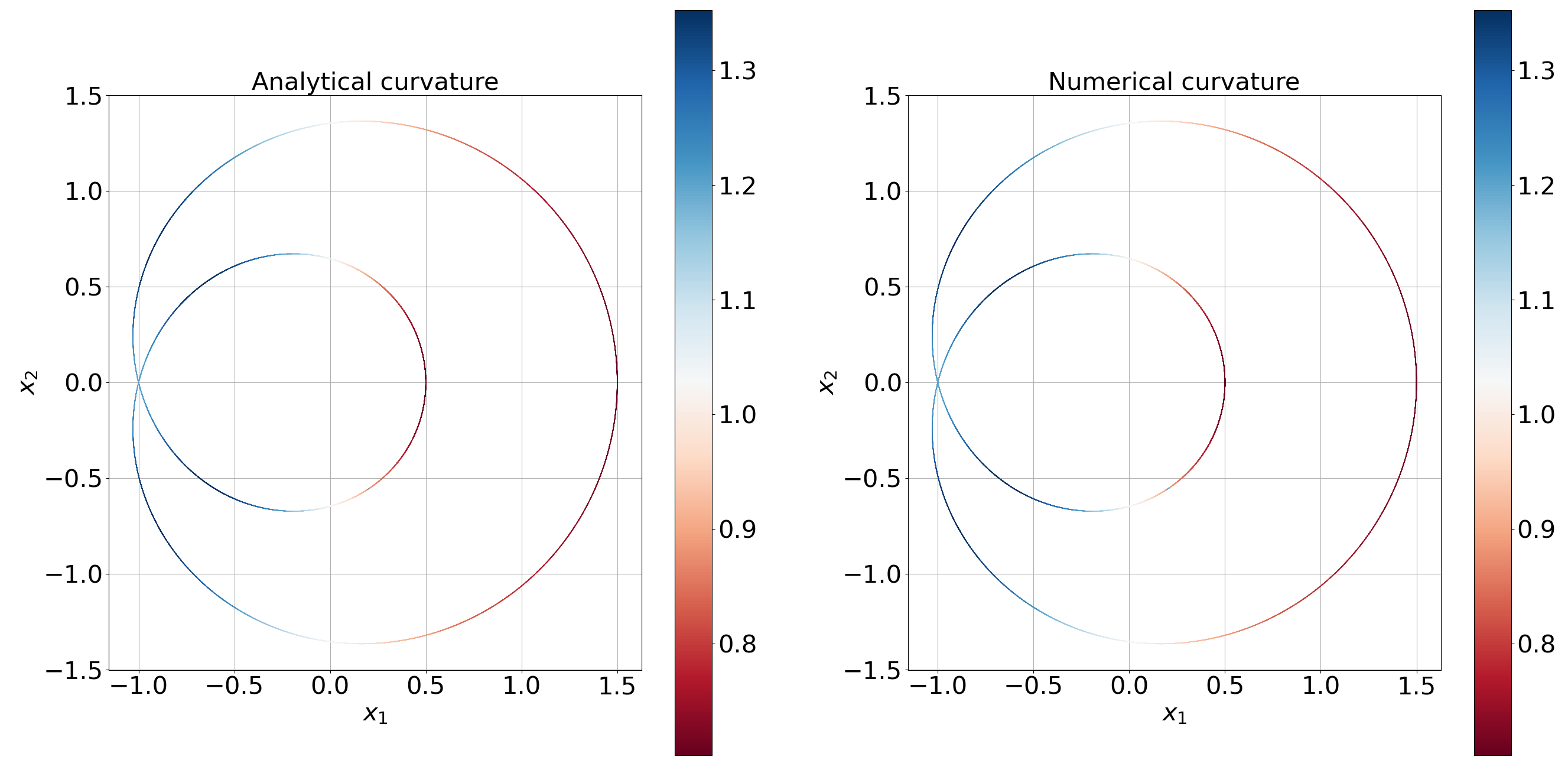
Consequently, the acceleration along the curve $\gamma(t)$, $\partial_{\gamma^{\prime}(t)}\gamma^{\prime}(t)$, must be in the direction of $W^{1}(\gamma(t))$. In particular, the acceleration in the direction of the unit tangent vector, $\partial_{\gamma^{\prime}(t)/\|\gamma^{\prime}(t)\|}(\gamma^{\prime}(t)/\|\gamma^{\prime}(t)\|)$, must match $W^{1}(\gamma(t))$. This is also clearly seen numerically. In Figure 2, each component of the two vector fields $\partial_{\gamma^{\prime}/\|\gamma^{\prime}\|}(\gamma^{\prime}/\|\gamma^{\prime}\|)$, computed analytically, and $W^{1}$, computed numerically using Eq. 19, are seen to coincide. Thus, the norms of the two vector fields are of course in close agreement as well, as can be seen in Figure 3. Both the analytically computed norm $\|\partial_{\gamma^{\prime}/\|\gamma^{\prime}\|}(\gamma^{\prime}/\|\gamma^{\prime}\|)\|$, and the numerically computed $\|W^{1}\|$ are shown as a colormap on the vector field $V^{1}=\gamma^{\prime}(t)/\|\gamma^{\prime}(t)\|$. The plots in Figure 3 are, a fortiori, a visualization of the curvature of the one-dimensional unstable manifold $\gamma(t)$. The final results of the analytical curvature calculations are provided in Appendix section B.

4.2 Numerical verification of the curvature of the Lorenz attractor

Next we consider the well-known Lorenz’63 system, given by the following system of ODEs:

$$\frac{d}{dt}\begin{bmatrix}{\rm x}_{1}\\ {\rm x}_{2}\\ {\rm x}_{3}\end{bmatrix}=F([{\rm x}_{1},{\rm x}_{2},{\rm x}_{3}]^{T}):=\begin{bmatrix}10({\rm x}_{2}-{\rm x}_{1})\\ {\rm x}_{1}(28-{\rm x}_{3})-{\rm x}_{2}\\ {\rm x}_{1}{\rm x}_{2}-\dfrac{8{\rm x}_{3}}{3}\\ \end{bmatrix}.$$ (22)

The map $\varphi$ is defined here to be a time-discretized form of the above system of ODEs. In particular, we use a second-order Runge-Kutta scheme with a time step of $\delta t=0.01$. The map $\varphi(x)=x_{1}$, is the time-integrated solution after time $\delta t$, starting from $x:=[{\rm x}_{1},{\rm x}_{2},{\rm x}_{3}]^{T}\in\mathbb{R}^{3}.$

Figure 4: Orbit points of the Lorenz system shown on the ${\rm x}_{1}$-${\rm x}_{3}$ plane, at $T_{1}=18$ (left) and at $T_{2}=20$ (right), colored according to the distance from their centroid normalized by the centroid $z$-coordinate. The initial conditions were 10001 equi-spaced points on the short line segment joining (-0.01,0,1) and (0.01,0,1).

Figure 5: Comparison between $V^{1}$ from an iteration of the tangent dynamics (shown in orange) and $V^{1}$ from finite difference of the primal trajectories (in blue). The first column shows the components of $V^{1}$ at time $T_{1}=18$ and the second column at $T_{2}=20.$ The first, second and third rows show the ${\rm x}_{1}$, ${\rm x}_{2}$, ${\rm x}_{3}$ components of $V^{1}$ respectively.

Figure 6: Comparison between $W^{1}$ from the differential CLV method (shown in orange) and $W^{1}$ from finite difference (in gray). The first column shows the components of $W^{1}$ at time $T_{1}=18$ and the second column at $T_{2}=20.$ The first, second and third rows show the ${\rm x}_{1}$, ${\rm x}_{2}$, ${\rm x}_{3}$ components of $W^{1}$ respectively.

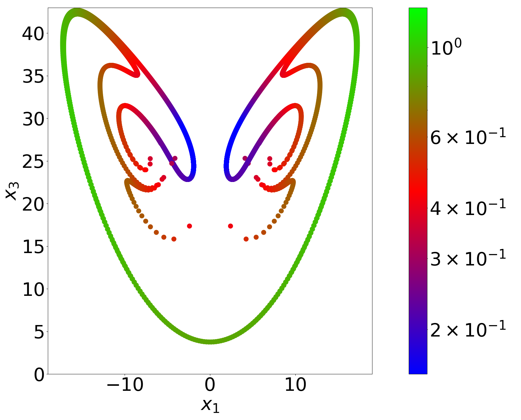
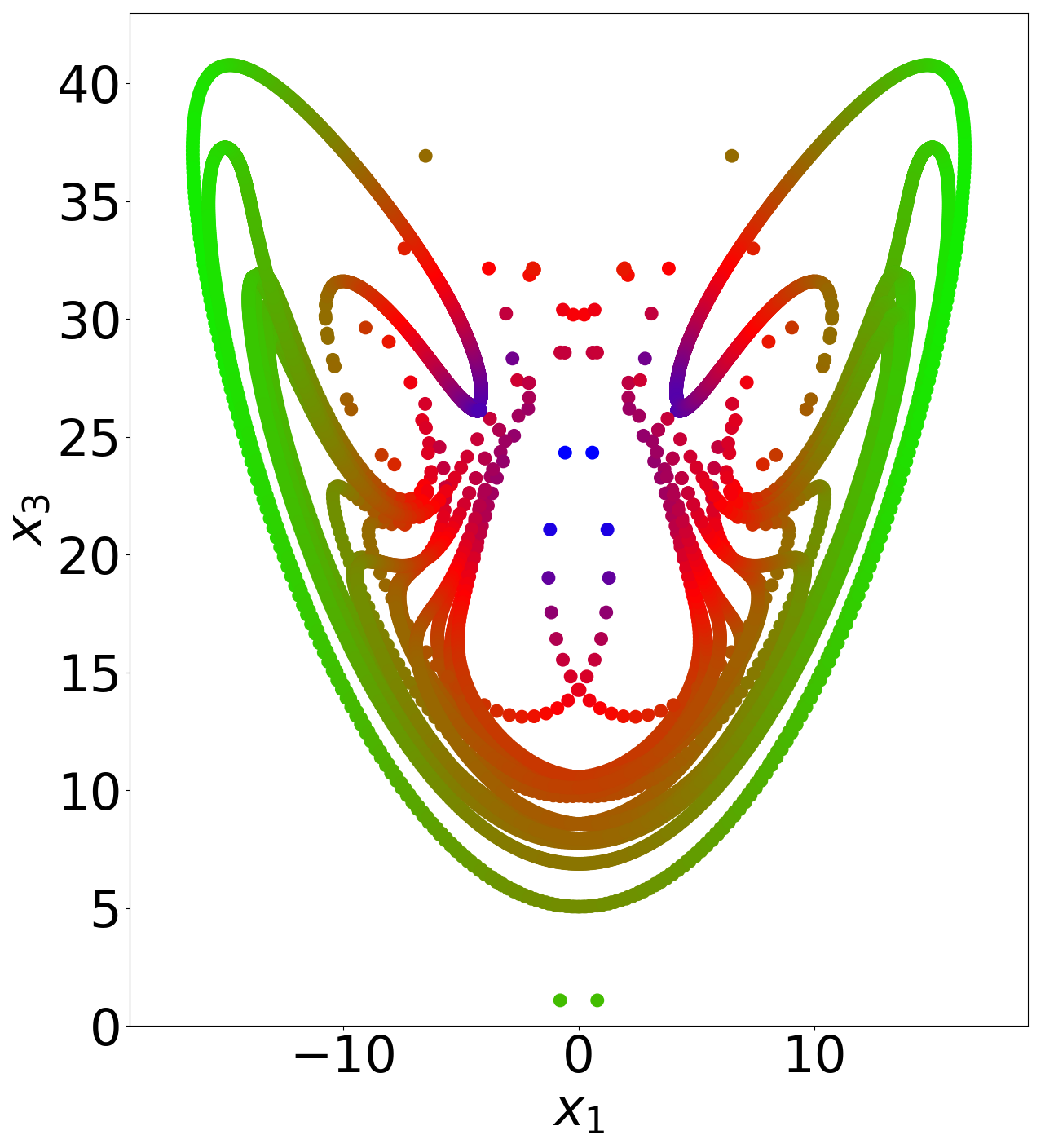
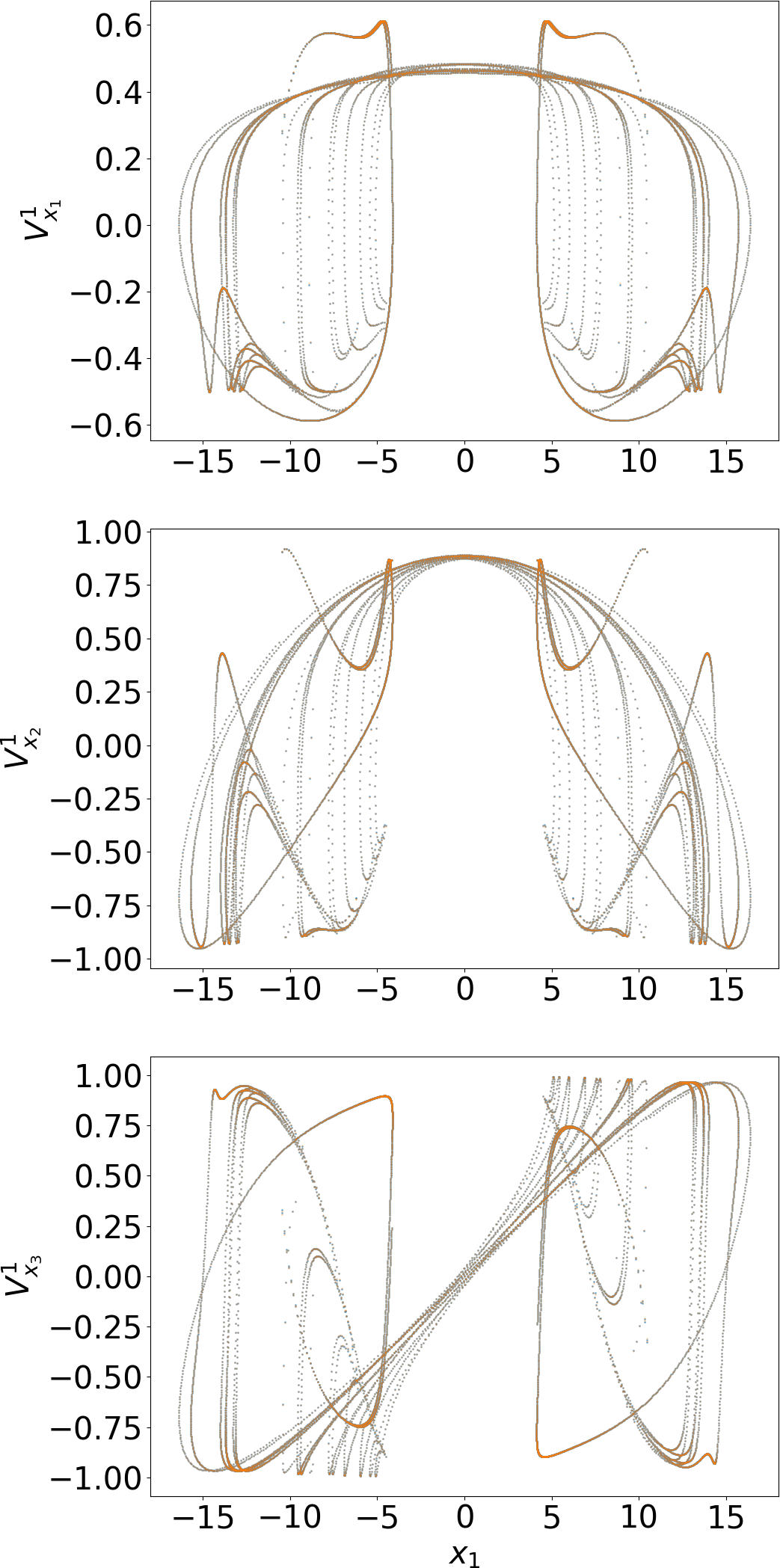
The Lorenz’63 map defined this way has the following Lyapunov exponents: $\lambda_{1}\approx 0.9$, $\lambda_{2}\approx 0$ and $\lambda_{3}\approx-14.6.$ The unstable manifold, which is tangent to the CLV corresponding to $\lambda_{1}$, is one-dimensional. There is a one-dimensional center manifold tangent to the right hand side of the ODE, $F$. This corresponds to $\lambda_{2}\approx 0$, i.e., since clearly $F(x_{1})\approx d\varphi_{x}F(x),$ the tangent vector roughly parallel to $F(x)\in T_{x}\mathbb{R}^{3}$ does not show exponential growth or decay under the tangent dynamics. Thus, this map is not uniformly hyperbolic as per the description in section 2.2. Rather, it is a partially hyperbolic system –a generalization of a uniformly hyperbolic system that allows a center direction – in which the center-unstable manifold is two-dimensional and tangent to ${\rm span}\left\{F\right\}\oplus E^{u}$. The Lorenz attractor nevertheless mimics the statistical behavior of a uniformly hyperbolic attractor. For instance, the central limit theorem holds for Hölder continuous observables and an SRB-type invariant distribution exists araujo .

In Figure 4, we numerically calculate the one-dimensional unstable manifold at $x:=(0,0,1)$ of the Lorenz attractor. We populate the small line segment connecting [-0.01,0,1] and [0.01,0,1] with 10001 equi-spaced initial conditions. In Figure 4, these points are shown after time evolution for time $T_{1}=18$ or $n_{1}=1800$ steps (on the left) and $T_{2}=20$ or $n_{2}=2000$ steps (on the right). The points that are a small distance from one another at all times up to the indicated times are considered orbits within local unstable manifolds of the reference orbit $\left\{x_{n}\right\}$.

Along these selected orbits, we use the following finite difference approximation to compute $V^{1}$:

$$V^{1}(y_{n})\approx\frac{x_{n}-y_{n}}{\left\lVert x_{n}-y_{n}\right\rVert}.$$ (23)

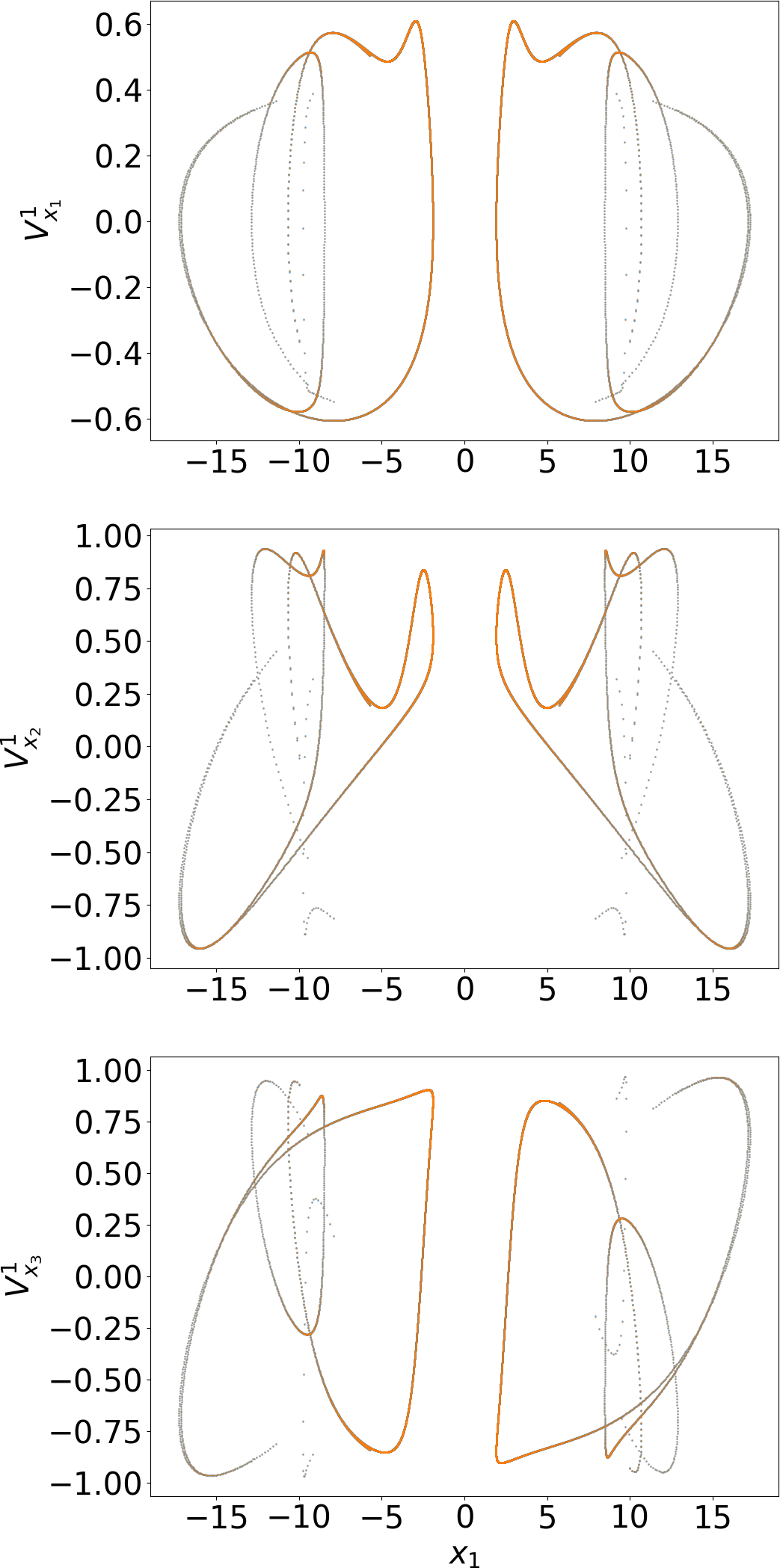
The 3 components $V^{1}_{{\rm x}_{i}}$, $i=1,2,3$ obtained this way are shown in gray in Figure 5; to avoid confusing these scalar fields with $V^{1}(x_{n})$, we do not use the shorthand notation, in this section, for $V^{1}(x_{n})$, which refers to the first CLV at the phase point $x_{n}$. The scalar fields $V^{1}_{{\rm x}_{i}}$ match match closely the results, shown in orange, of a more typical method of computing the first CLVs. This second method to compute $V^{1}(x_{n})$ uses only the trajectory $x,x_{1},\cdots,x_{n}$ and the tangent dynamics along this trajectory, and works as follows: randomly initialize $v(x)$ and propagate the tangent dynamics with repeated normalization.

$$v(x_{n+1}) =d\varphi(x_{n})v(x_{n}),$$ (24)

$$v(x_{n+1}) \longleftarrow v(x_{n+1})/\|v(x_{n+1})\|.$$ (25)

Carrying this out for $n\in\mathbb{Z}^{+}$, similar to a power iteration method for the computation of the dominant eigenvector of a matrix, yields a unit vector $v(x_{n})$ that aligns with $V^{1}(x_{n}).$ As confirmed in Figure 5, this procedure is equivalent to the above-mentioned finite difference procedure, as long as $y_{n}$ is in a small neighborhood of $x_{n},$ for the length of the trajectory considered.

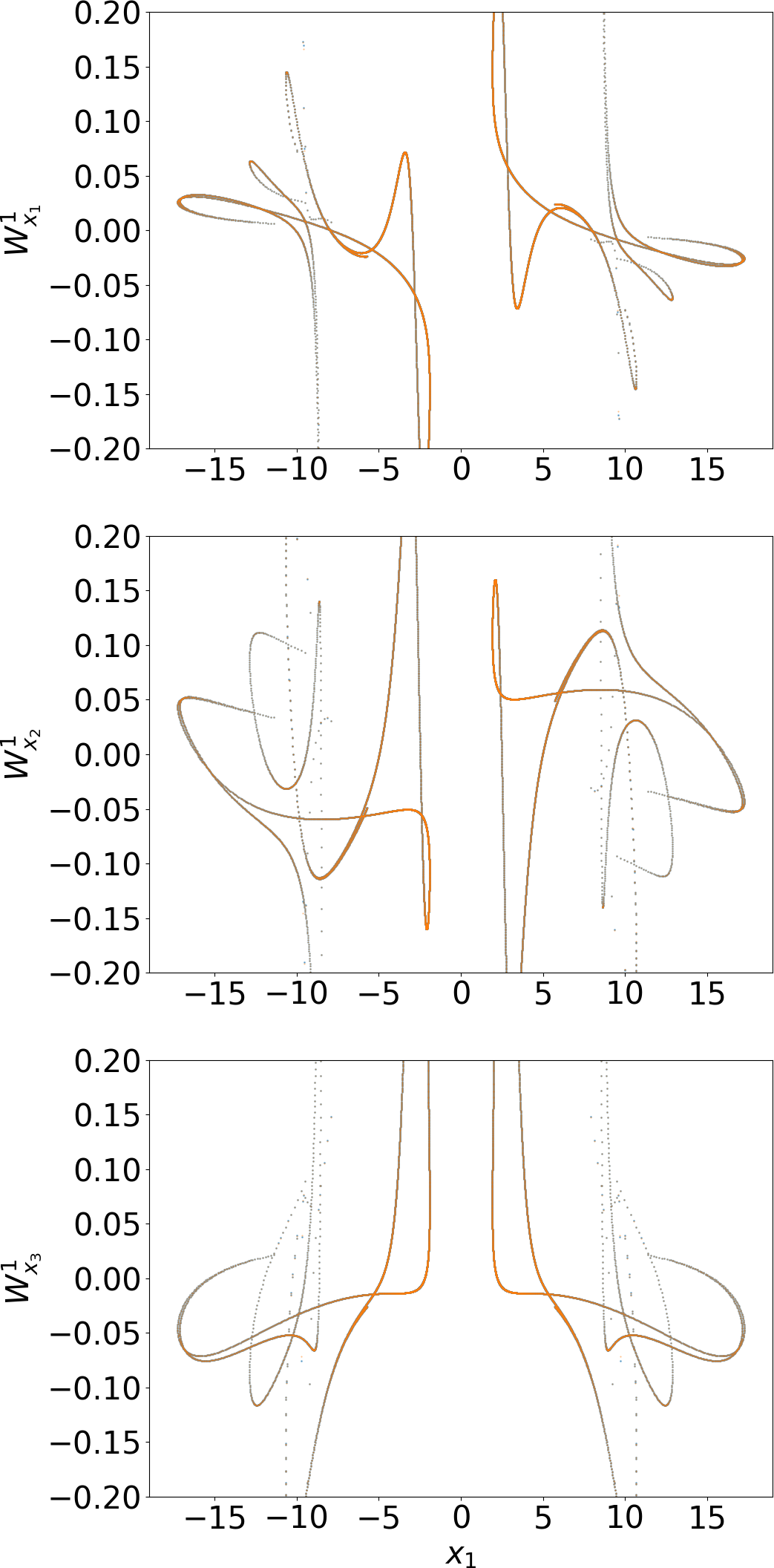
Having visualized $V^{1}$ along trajectories, we now compute $W^{1}$ using our differential CLV method in section 3. To test its correctness, we also compute $W^{1}$ using a finite difference method as follows. As usual, let the reference trajectory along which we require to compute $W^{1}$ be $x,x_{1},\cdots,x_{N},$ and assume that we know the CLVs $V^{1}(x),V^{1}(x_{1}),\cdots,V^{1}(x_{N}).$ Let $y,y_{1},\cdots,y_{N}$ and $r,r_{1},\cdots,r_{N}$ be two other trajectories that are at most a distance of ${\cal O}(1)$ away from the reference trajectory, at each of the $N$ time steps. Then, according to our preceding discussion,

$$V^{1}(y_{n})\approx-V^{1}(x_{n})\approx\frac{x_{n}-y_{n}}{\left\lVert x_{n}-y_{n}\right\rVert}.$$ (26)

At each $n$, we rescale $y_{n}$ and $r_{n}$ along $V^{1}(x_{n})$ to obtain the two points i) $\tilde{y}_{n}=x_{n}+\epsilon_{y_{n}}V^{1}(y_{n})$, ii) $\tilde{r}_{n}=x_{n}+\epsilon_{r_{n}}V^{1}(r_{n})$. Then, we can approximately compute $W^{1}(x_{n})$ as

$$W^{1}(x_{n})\approx\frac{(\tilde{r}_{n}-x_{n})/\epsilon_{r_{n}}-(\tilde{y}_{n}-x_{n})/\epsilon_{y_{n}}}{\left\lVert\tilde{r}_{n}-\tilde{y}_{n}\right\rVert}.$$ (27)

In Figure 6, we plot the three components of $W^{1}$: $W^{1}_{{\rm x}_{1}},W^{1}_{{\rm x}_{2}},W^{1}_{{\rm x}_{3}}$ computed using the above procedure in gray and the same quantity computed using the differential CLV algorithm in section 3 in orange. The closeness of the two results indicates the correctness of our algorithm. It is also a numerical verification of the fact that $V^{1}$ is differentiable along itself in this system, even though it is only partially hyperbolic.

4.3 Qualitative verification on a perturbed cat map

We consider a smoothly perturbed Cat map (PCM) (see section 2.3) due to Slipantschuk et al. julia . The PCM julia was designed to be an analytic, area-preserving, uniformly hyperbolic map of the torus, whose spectral properties can be computed analytically. The PCM is given by

$$\varphi([{\rm x}_{1},{\rm x}_{2}])=\begin{bmatrix}2&1\\ 1&1\end{bmatrix}\begin{bmatrix}{\rm x}_{1}\\ {\rm x}_{2}\end{bmatrix}+\begin{bmatrix}\Psi_{s_{1},s_{2}}({\rm x}_{1})\\ \Psi_{s_{1},s_{2}}({\rm x}_{1})\end{bmatrix},$$ (28)

where

$$\Psi_{s_{1},s_{2}}(y):=(1/\pi)\arctan\Big{(}s_{1}\sin(2\pi y-s_{2})/(1-s_{1}\cos(2\pi y-s_{2}))\Big{)}$$

is a perturbation whose maximum magnitude is controlled by the parameter $s_{1}$ and the location of the maximum, by $s_{2}.$ Clearly, the original Cat map is recovered at $s_{1}=0.$ As in the Cat map, the sum of the LEs is 0 but their values are sensitive to the parameters, with lesser sensitivity to $s_{2}$ when compared to $s_{1}$. Unlike the Cat map, the CLVs are no longer uniform in phase space and are also not orthogonal to each other. In Figure 7, we show the vector fields $V^{1}$ and $V^{2}$ computed at $s_{1}=0.75$ and $s_{2}=0.2.$ Notably, non-zero values of $s_{1}$ create a curvature in the CLVs, which is again non-uniform in space.

Figure 7: The vector fields $V^{1}$ (left) and $V^{2}$ (right) are shown for the PCM at $s_{1}=0.75,s_{2}=0.2$.

Figure 8: The vector field $V^{1}$ is shown for the PCM at $s_{1}=0.75,s_{2}=0.2$. The color represents the values of $\|W^{1}\times V^{1}\|$, which equals the norm of $\|W^{1}\|$ multiplied by a sign representing the orientation with respect to $V^{1}$.

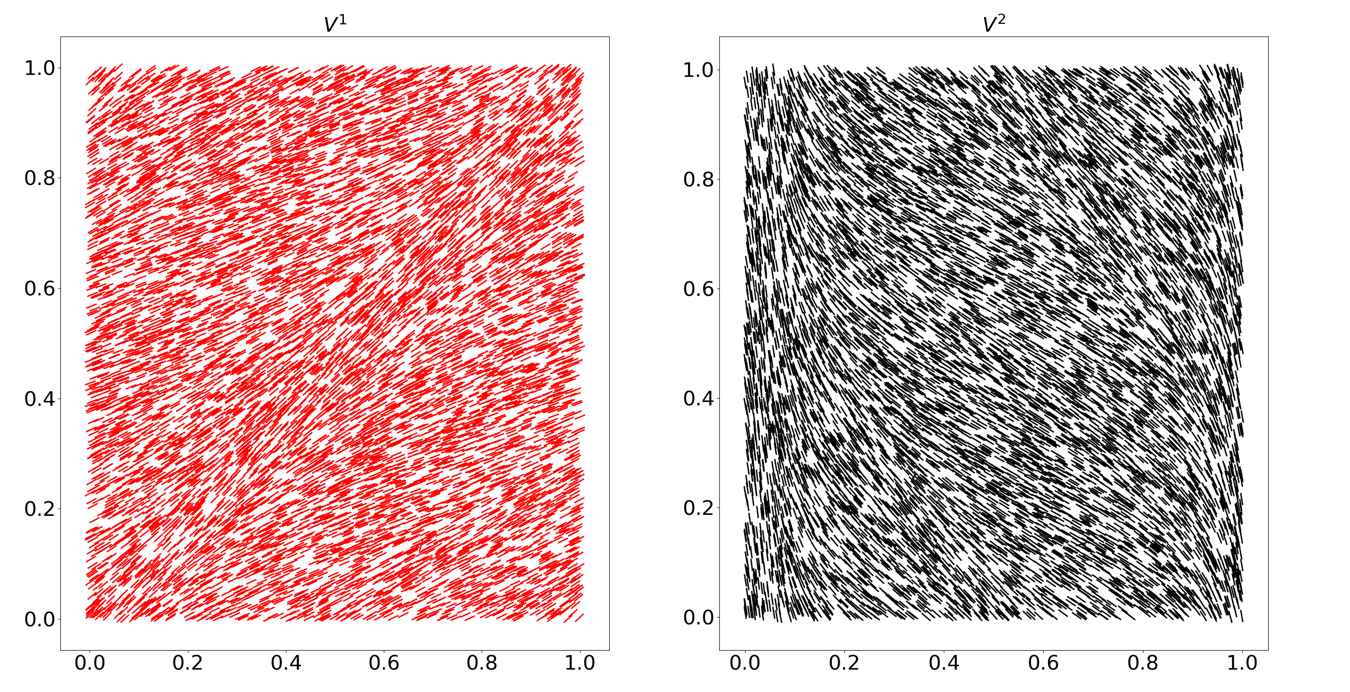
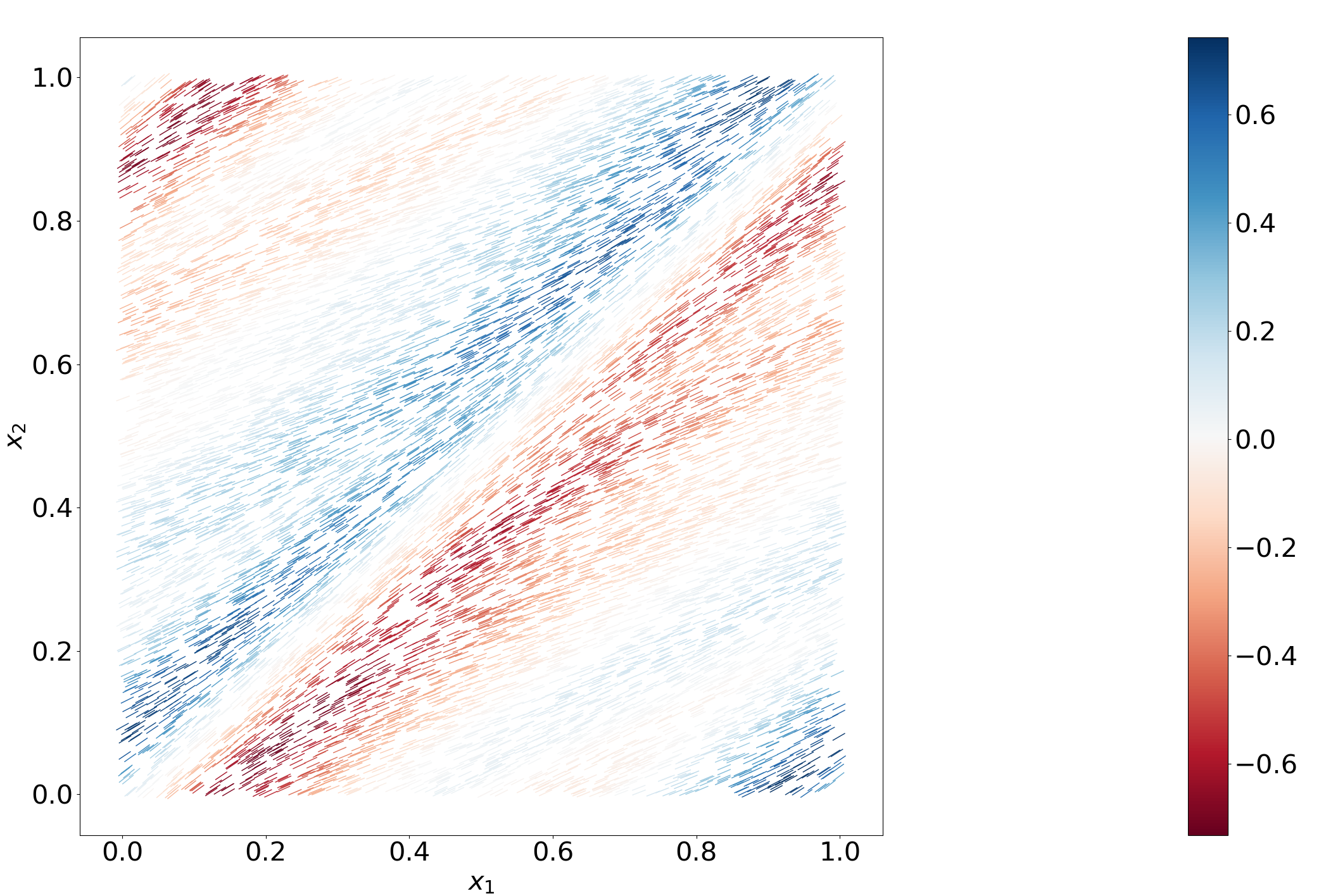
We compute the self-derivative of the unstable CLV using our differential CLV method in section 3. By construction, the method produces a vector field $W^{1}$ that is orthogonal to $V^{1}$. The norm of the computed vectors, $\|W^{1}\|$, is shown signed according to its orientation with respect to $V^{1}.$ In particular, in Figure 8, we plot $\|W^{1}\times V^{1}\|$ as a colormap on the vector field $V^{1}.$ Figure 8 is a qualitative representation of the fact that $\left\lVert W^{1}\right\rVert$ is the curvature of the unstable manifold, which is everywhere tangent to the plotted vector field $V^{1}.$ The $V^{1}$ self-derivative $W^{1}$ is the acceleration of a particle moving with the velocity field $V^{1}$. This intuitive picture is mirrored by Figure 8, in which $\left\lVert W^{1}\right\rVert$ is higher in regions of velocity changes than where the velocity appears rather uniform (e.g. in a thin strip around the diagonal of the square). The regions of similar magnitude of acceleration but of opposite sign, reflect the symmetry in the velocity field $V^{1}$ about $x_{1}=x_{2}$, and moreover indicate the opposite directions of the turns made in those regions by traveling particles.

4.4 Qualitative verification on the volume-decreasing perturbed Cat

While the PCM was an example of a symplectic uniformly hyperbolic system, now we consider a dissipative uniformly hyperbolic map. We introduce another perturbed Cat map, with smooth nonlinear perturbations that cause the resulting map to be volume-decreasing. The norm of the perturbations is controlled by a set of four parameters $s=[s_{0},s_{1},s_{2},s_{3}]^{T}$ and the unperturbed Cat map (the original Anosov Cat) is recovered at $s=[0,0,0,0]$. The map, referred to as the dissipative Cat map or DCM hereafter, is defined as follows:

$$\varphi([{\rm x}_{1},{\rm x}_{2}]^{T}) =\begin{bmatrix}2&1\\ 1&1\end{bmatrix}\begin{bmatrix}{\rm x}_{1}\\ {\rm x}_{2}\end{bmatrix}+\left(s_{0}\begin{bmatrix}v_{0}\\ v_{1}\\ \end{bmatrix}+s_{1}\begin{bmatrix}v_{2}\\ v_{3}\end{bmatrix}\right)\sin(2\pi\tilde{V}^{2}\cdot x)/c$$

$$+\left(s_{2}\begin{bmatrix}v_{0}\\ v_{1}\\ \end{bmatrix}+s_{3}\begin{bmatrix}v_{2}\\ v_{3}\end{bmatrix}\right)\sin(2\pi\tilde{V}^{1}\cdot x)/c$$ (29)

where $\tilde{V}^{2}:=[v_{0},v_{1}]^{T}=[5,-8]^{T}\in\mathbb{R}^{2}$ is a rational approximation of the stable CLV of the unperturbed Cat map. Similarly, $\tilde{V}^{1}:=[v_{2},v_{3}]^{T}=[8,5]^{T}\in\mathbb{R}^{2}$ is a rational approximation of the unstable CLV of the unperturbed Cat map. The constant $c$ serves to normalize the perturbations and is set to $c=2\pi(v_{0}^{2}+v_{1}^{2}).$

Figure 9: The vector field $V^{1}$ is shown for the DCM at different parameter choices. The parameters not indicated are set to 0 in each case.

Figure 10: The vector field $V^{1}$ is shown for the DCM, colored according to $\left\lVert W^{1}\times V^{1}\right\rVert$. The parameters not indicated as 1 are set to zero in each case.

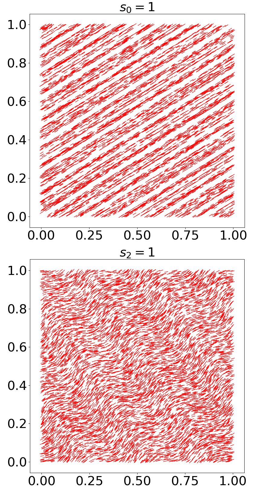
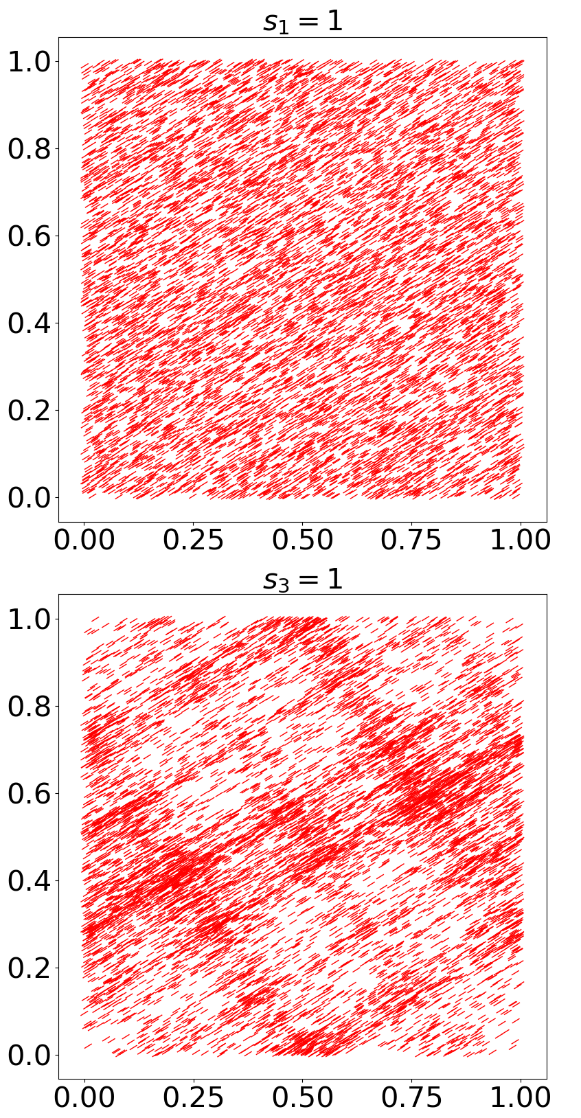
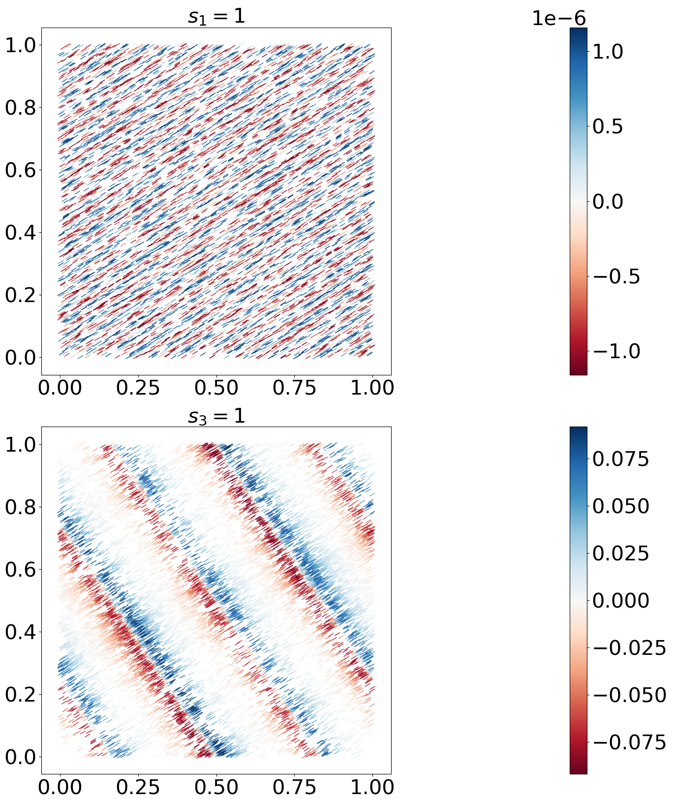
The four parameters together determine the norm and direction of the perturbation. In Figure 9, $V^{1}$ in plotted in each case of turning on just one of the four parameters, in order to isolate its effects. Each subfigure reflects the effect of a single parameter on $V^{1}$, in comparison to the unperturbed Cat map (in which $V^{1}$ is roughly parallel to the line $\tilde{V}^{1}$). For instance, when $s=[1,0,0,0]^{T}$, a perturbation is applied along the direction $\tilde{V}^{2}$, which is approximately along the stable direction of the DCM. The norm of this perturbation varies sinusoidally with the orientation along the approximately stable direction, $\tilde{V}^{2}$. As can be seen in the top-left of Figure 9, the CLV $V^{1}$ is rather uniform in its own direction but shows a striated pattern in the perpendicular direction, roughly along $\tilde{V}^{2}.$ As another example, the bottom-left subfigure shows $V^{1}$ at $s=[0,0,1,0]^{T}.$ From Eq. 29, we know that $s_{2}$ being non-zero introduces a perturbation, along $\tilde{V}^{2}$, whose norm varies in the approximately unstable direction, $\tilde{V}^{1}.$ This is portrayed in the figure, wherein $V^{1}$ appears as waves, which are seen traveling approximately along $\tilde{V}^{2}$ but the amplitudes of the waves clearly vary in the perpendicular, approximately unstable direction. Turning on the parameter $s_{1}$ exchanges the roles of $\tilde{V}^{1}$ and $\tilde{V}^{2}$ when compared to when $s_{2}$ is non-zero. From the top-right subfigure in which the effect of $s_{1}$ is shown, we can see that there is no noticeable curving of the unstable manifold since the perturbation is aligned with the unstable direction. Finally, the effect of a non-zero $s_{3}$ is depicted in the bottom-right of Figure 9. Here we see the compression and expansion of unstable manifolds in the unstable direction since a perturbation non-uniform in the unstable direction is applied along the unstable direction.

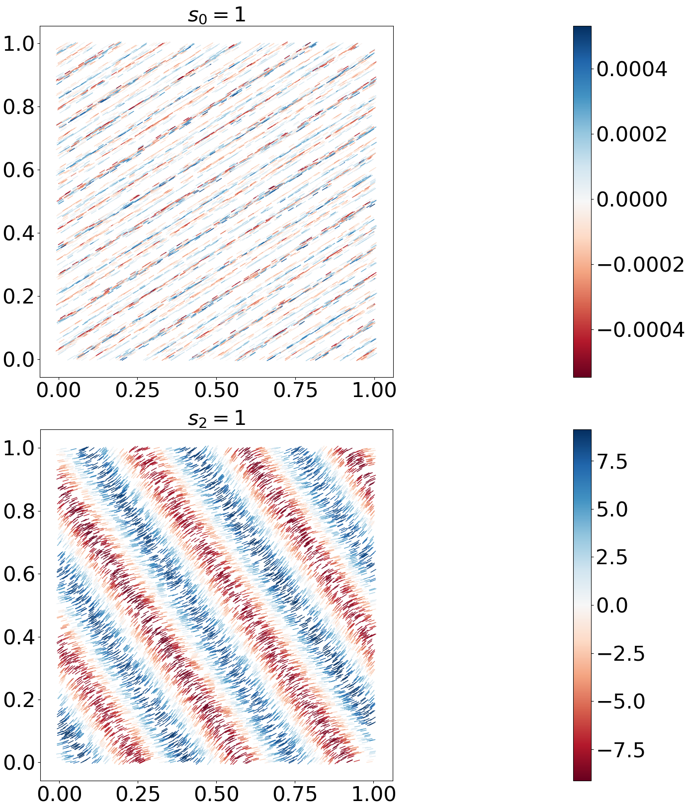
With this understanding of the effect of each parameter, we expect that $V^{1}$ would show a smaller sensitivity, in its own direction, when the norm of the perturbation is uniform along $\tilde{V}^{1}$. This is the case when $s_{2},s_{3}$ are set to 0. This intuition is confirmed by the numerical results obtained on using the differential CLV method. As shown in Figure 10, when either $s_{0}=1$ or $s_{1}=1$, and the other 3 parameters are set to 0, we see that the numerically computed $W^{1}$ has a smaller norm, when compared to the other cases.

On the bottom row in Figure 10 are the vector fields $W^{1}$ when either $s_{2}$ or $s_{3}$ are set to 1 and the rest to 0. In these cases, the norm of the perturbation varies along the approximately unstable direction, and this is clearly reflected in the higher (when compared to the other two cases) magnitudes of $W^{1}$. In addition, the variation in $W^{1}$ itself, which gives information about the second-order derivative of $V^{1}$, is also consistent with our expectations. For instance, $W^{1}$ shows a marked variation along $V^{1}$ when $s_{2}=1$ (bottom-left of Figure 10). This can be explained by the applied perturbations being sinusoidal in the direction of $\tilde{V^{1}}$, giving rise to a harmonic functions for the higher-order derivatives along $V^{1}$ as well. Finally, when $s_{3}=1$, (bottom-right of Figure 10), it is easy to observe that, qualitatively, the density of the lines $V^{1}$ is reflected in the magnitudes of $W^{1}$. This is not a coincidence, as we shall see in section 5. There, we describe that $W^{1}$ is indirectly related to the variation in the density of the SRB measure on the unstable manifold, due to perturbations along $V^{1}$. Now we can see that especially the $s_{3}=1$ case provides a visualization consistent with this theoretical insight. Particularly, the pronounced variation in the unstable direction (bottom-right, Figure 10), mirrors the changes in probability density on the unstable manifold, which is qualitatively measured by the closeness of the $V^{1}$ lines in Figure 9.

4.5 Numerical results on the Hénon map

As our final example, we consider the classical Hénon attractor. The Hénon map is the canonical form for a two-dimensional area-decreasing quadratic map henon :

$$\varphi([{\rm x}_{1},{\rm x}_{2}]^{T})=\begin{bmatrix}{\rm x}_{2}+1-s_{0}{\rm x}_{1}^{2}\\ s_{1}{\rm x}_{1}\end{bmatrix}.$$ (30)

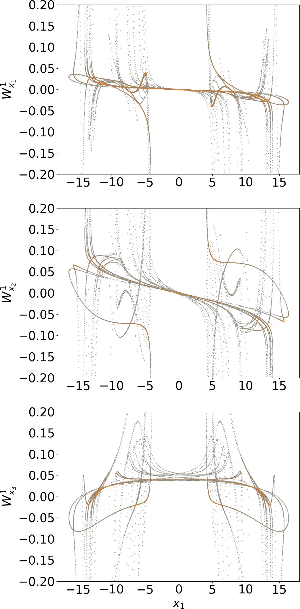
Taking the parameters $s_{0}$ and $s_{1}$ at their standard values of $s_{0}=1.4$ and $s_{1}=0.3$, we obtain the Hénon attractor, on which the CLVs are shown in Figure 11. At these parameter values, the Hénon attractor is nonhyperbolic due to the presence of tangencies between the stable and unstable manifolds henon-hyperbolicity . On this map, we apply the differential CLV method we derived in section 3, and the resulting $W^{1}$ is shown in Figure 12. The CLVs may not be differentiable everywhere, as seen by the large magnitudes of the numerically computed $W^{1}$ at the sharp turns in the attractor.

Figure 11: The CLV $V^{1}$ on the henon attractor. Inset is the CLV field in a neighborhood of the fixed point $\approx(0.63,0.19).$

Figure 12: The vector field $V^{1}$ is shown for the Hénon map. The color represents the $V^{1}$ self-derivative norm, $\|W^{1}\|.$

Figure 13: The vector field $V^{1}$ is shown for the Hénon map. The color represents $\|W^{1}\|$, the curvature of the unstable manifold.

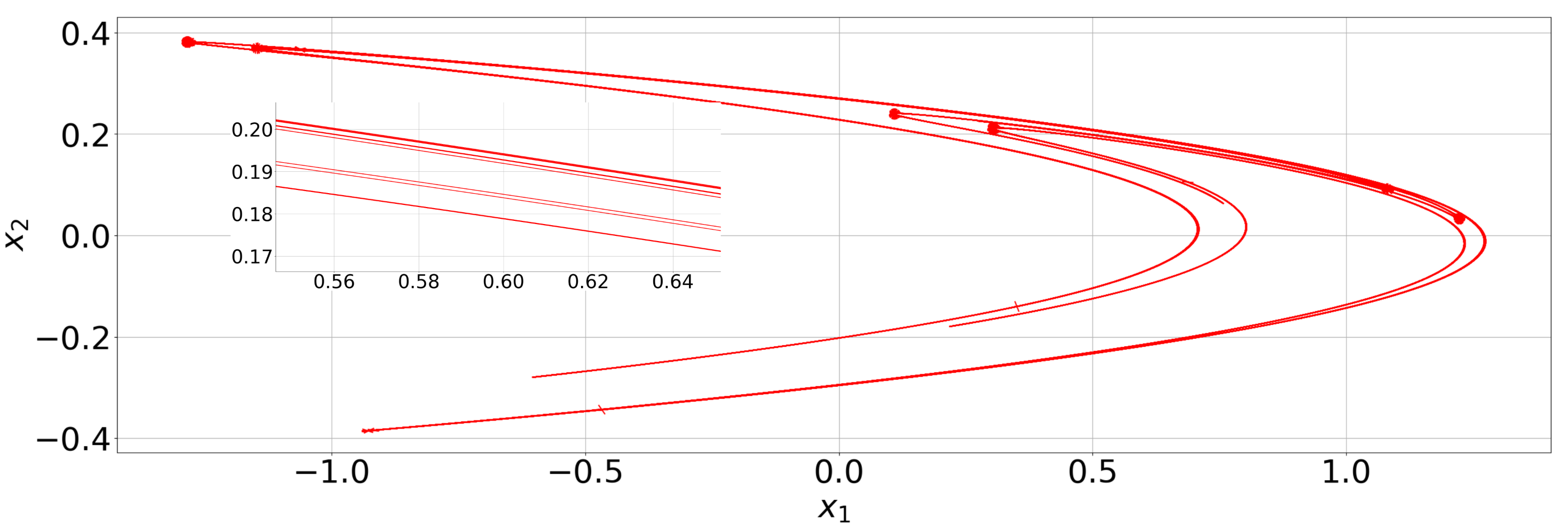
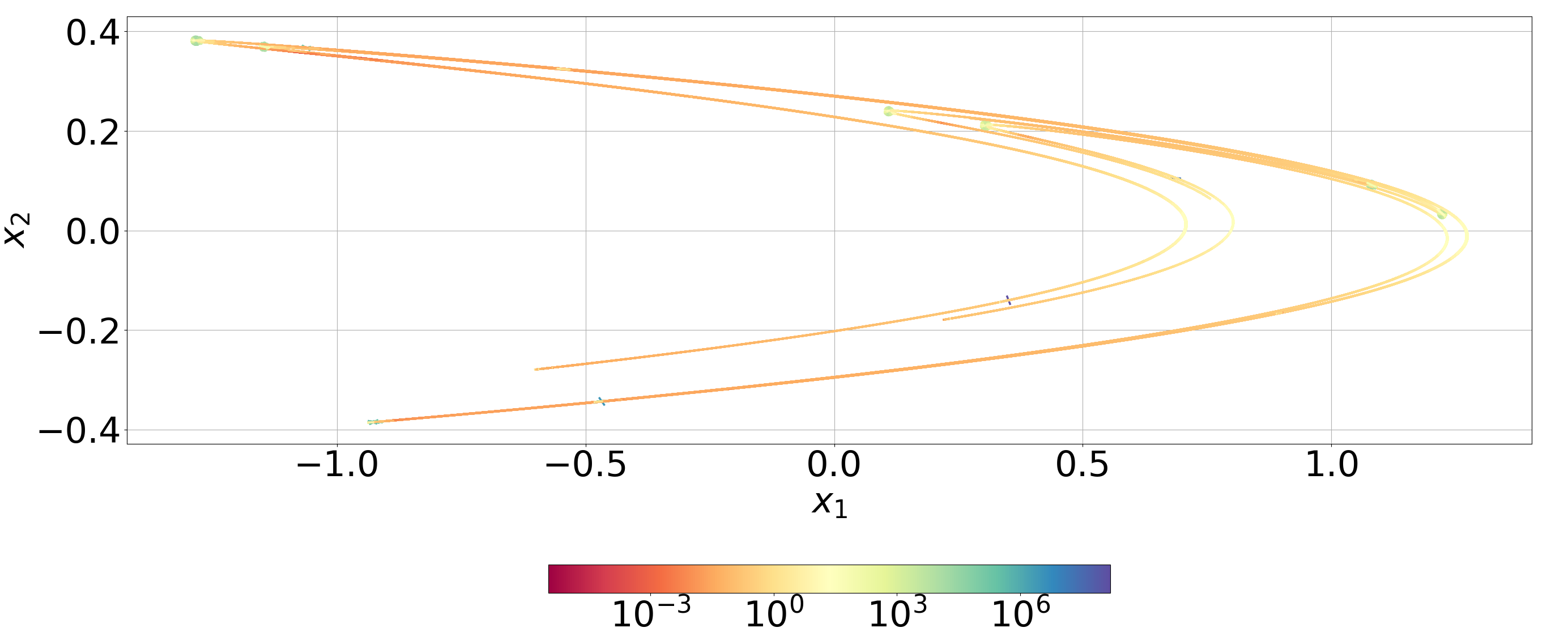
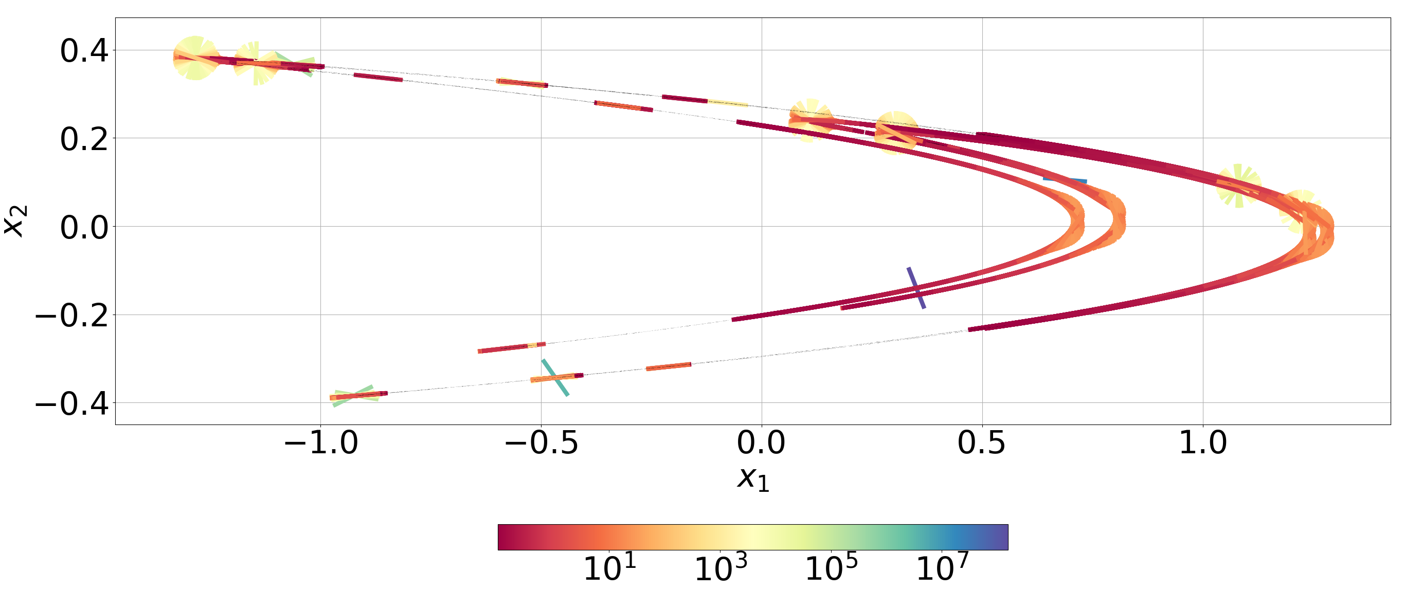
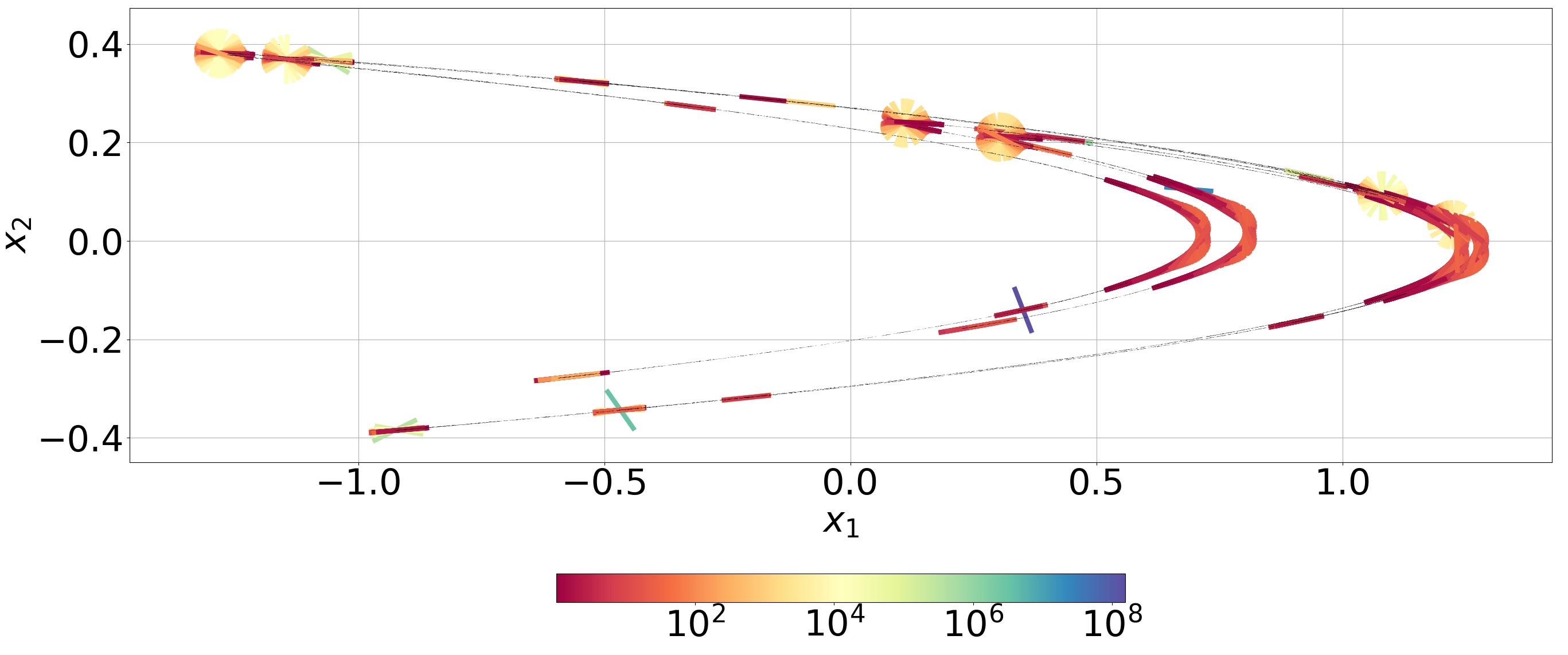
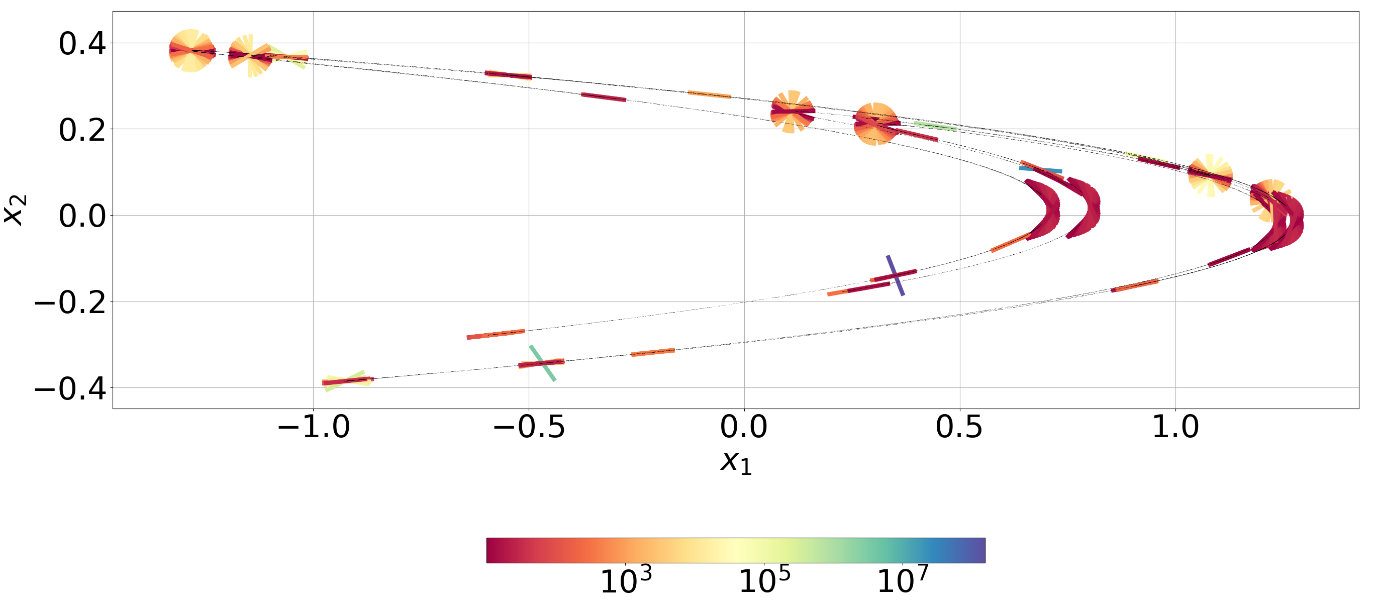
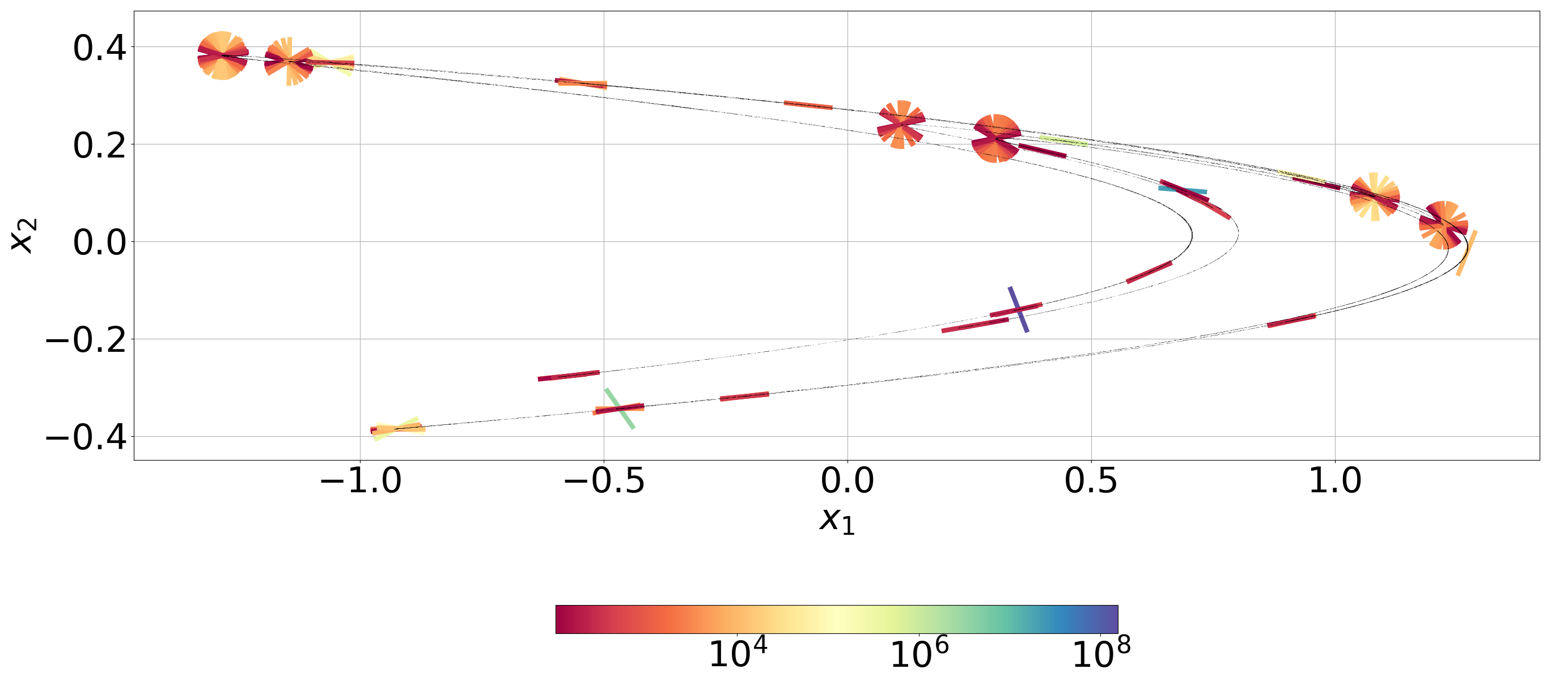
In Figure 13, we dissect the derivatives further to investigate the issue of differentiability numerically. In each subfigure, the vector field $V^{1}$ is plotted colored according to $\|W^{1}\|;$ at the points at which $\|W^{1}\|$ is not in the range indicated by the colormap, $V^{1}$ is shown using thin black lines. From the top row of Figure 13, it is clear that $\|W^{1}\|<0.1$ for the relatively straight portions of the attractor and the points on the right, curved side of the attractor, still have a curvature less than 1. On the bottom row, the more rounded portions of the attractor, as expected, have a higher curvature when compared to the previous cases. On the bottom-right, we see that only the corners and turns have $\|W^{1}\|$ higher than 100. Among these points, the variation in the curvature, $\|W^{1}\|$, is over six orders of magnitude, with the sharp corners having the highest curvatures. In this case, our numerical method for $W^{1}$ acts as an indicator for the lack of differentiability at some points. At least in two dimensions, this also turns out to be a detector for uniform hyperbolicity, based on our discussion in section 2.4.

5 An application of CLV derivatives to statistical linear response

A landmark result in the theory of uniformly hyperbolic systems due to Ruelle (ruelle ruelle1 ; gouezel contains a modern proof of the result) is the smooth response of their statistics to parameter perturbations. Here we briefly describe this result, called the linear response formula, and draw a connection between the formula and Eq. 17, which is the differential expansion equation.

Consider a family of uniformly hyperbolic maps $\varphi_{s}\in C^{3}(\mathbb{M})$, where $s$ is a small parameter around 0. Let the reference map $\varphi_{0}$ be written simply as $\varphi$, and $V$ be a smooth vector field such that $\varphi_{s}=\varphi+sV$ up to first order in $s$. Let the SRB measure of $\varphi_{s}$ be $\mu_{s}$: that is, $\mu_{s}$ is a $\varphi_{s}$-invariant probability distribution on $\mathbb{M}$ such that for any continuous scalar observable $J$, the ergodic average starting from a $x\in\mathbb{M}$ Lebesgue-a.e., $\lim_{N\to\infty}(1/N)\sum_{n=0}^{N-1}J(\varphi_{s}^{n}(x))=\langle J,\mu_{s}\rangle.$

Ruelle’s linear response theory ruelle ruelle1 proves the existence of the statistical response to parameter changes, $\langle J,\partial_{s}\mu_{s}\rangle$, in uniformly hyperbolic systems, including expressing this quantity as an exponentially converging series, which is known as linear response formula. The quantity $\langle J,\partial_{s}\mu_{s}\rangle$ represents the derivative with respect to $s$ of ergodic averages or equivalently ensemble averages of observables with respect to the SRB measure, and is of immense interest in practical applications. The statistical sensitivity $\langle J,\partial_{s}\mu_{s}\rangle$ is useful for sensitivity analysis, uncertainty quantification, model selection etc, in every scientific discipline from climate studies lucarini_climate lucarini to aerodynamic fluid flows angxiu-jfm francisco nisha-shadowing . The linear response formula ruelle ruelle1 is as follows:

$$\langle J,(\partial_{s}\mu_{s})\Big{|}_{0}\rangle =\sum_{n=0}^{\infty}\langle d(J\circ\varphi^{n})\cdot V,\mu_{0}\rangle.$$ (31)

Although the above series is exponentially converging, previous works nisha_ES eyink suggest that it is computationally infeasible to calculate the series in its original form when $V$ has a non-zero component in $E^{u}$, especially in high-dimensional practical systems. This is because the integrand in each term increases exponentially with $n$: $|d(J\circ\varphi^{n})\cdot V|\sim{\cal O}(\exp(\lambda_{1}n))$, for almost every perturbation $V$, which will have a non-zero component along $V^{1}$. If each term in the series is regularized by an integration by parts, the resulting form of the linear response formula is more amenable to computation.

For a simple illustration, we consider the case of one-dimensional unstable manifolds, and fix the smooth perturbation field to be $V=a\>V^{1}$, which has a scalar component, $a$, along the unstable CLV. Applying integration by parts to Eq. 31 on the unstable manifold ruelle ruelle1 (see also Appendix section D), and then using the fact that ergodic averages converge to ensemble averages for Lebesgue-a.e. $x$,

$$\langle J,(\partial_{s}\mu_{s})\Big{|}_{0}\rangle =-\sum_{k=0}^{\infty}\lim_{N\to\infty}\dfrac{1}{N}\sum_{n=0}^{N-1}J(x_{k+n})\>(a(x_{n})\>g(x_{n})+b(x_{n}))$$ (32)

where

• $\rho_{0}$ is the density of the conditional distribution of $\mu_{0}$ on unstable manifolds srb ;

• $g(x):=\dfrac{1}{\rho_{0}(x)}\dfrac{d(\rho_{0}\circ\mathcal{C}_{x,1})(t)}{dt}\Big{|}_{t=0},$ is the logarithmic density gradient function; and,

• $b(x):=\dfrac{d(a\circ\mathcal{C}_{x,1})(t)}{dt}\Big{|}_{t=0},$ is the derivative of $a$ along unstable manifolds.

The computational infeasibility of Ruelle’s original expression in Eq. 31 is overcome by Eq. 32, as it results from regularization through integration by parts. That is, the ergodic averaging computation, listed in Eq. 32, follows the central limit theorem, with an error convergence as ${\cal O}(1/\sqrt{N})$, when computed along an orbit of length $N$. To compute Eq. 32, we must determine the two functions $g$ and $b$ along orbits. The derivative $b$ can be computed at any $x_{n}$ as $b(x_{n})=(V^{1}_{n})^{T}(dV)_{n}\>V^{1}_{n}$; to derive this expression, we use the fact that $W^{1}\cdot V^{1}=0$, which follows from Eq. 19. Now, the only other unknown is the fundamental quantity – the logarithmic density gradient denoted $g$. Using the fact that $\varphi$ preserves $\mu_{0}$, it can be shown that (see section 4 of nisha-s3 for an alternative derivation and adam for an intuitive description of $g$ on one-dimensional unstable manifolds) $g$ satisfies the following iterative equation along trajectories:

$$g_{n+1}=\dfrac{g_{n}}{z_{n,1}}+\alpha_{n,1}.$$ (33)

In the above equation, we use the shorthand notation $g_{n}:=g(x_{n})$ and $z_{n,1}:=z_{x_{n},1}$, fixing any $\mu_{0}$-typical $x$. Thus, Eq. 33 is an iterative formula that can be used to compute $g$ along orbits. It uses the differential expansion equation (Eq. 17) for the second term on the right hand side. The values of $g$ along a typical orbit, thus computed, are used in Eq. 32 to obtain the desired sensitivity.

6 Conclusion

In this work, we have derived a numerical method, called the differential CLV method, to compute the derivatives of Covariant Lyapunov Vectors along their own directions: the CLV self-derivatives. These directional derivatives exist in smooth uniformly hyperbolic systems with compact attractors. The differential CLV method converges asymptotically at an exponential rate in the case of the CLV self-derivatives corresponding to the largest and smallest Lyapunov exponents. We demonstrate the application of the differential CLV method on a variety of systems with one-dimensional unstable manifolds including a quasi-hyperbolic attractor (Lorenz’63) and a non-hyperbolic attractor (Hénon). In the two-dimensional uniformly hyperbolic systems considered, including perturbations of the Cat map, our method provides rich visualizations of the curvature of the one-dimensional unstable manifold. A byproduct of the differential CLV method, without the orthogonal projection step (Eq. 19), known as the differential expansion equation (Eq. 17), is fundamentally linked to the statistical linear response of a chaotic attractor. The link is through its utility to compute the divergence of perturbations on the unstable manifold, with respect to the SRB measure conditioned on unstable manifolds. This connection makes the differential expansion derivatives concretely useful for efficiently differentiating statistics with respect to system parameters in uniformly hyperbolic systems. The differential CLV method does not have unconditional asymptotic convergence for the self-derivatives of all CLVs, but only the most unstable and the most stable CLVs, which are treated in this work. With sufficient generalization, however, the second-order tangent equations presented in this paper can spawn applications to sensitivity analysis in chaotic systems, and beyond.

Acknowledgments: We offer our sincere thanks to Dr. Jizhou Li and anonymous reviewers for helpful comments on this manuscript.

Appendix A The lack of differentiability of CLVs

In general, we say that a subspace $E$ is Hölder continuous on $\mathbb{M}$ if there exist constants $K,\delta>0$ and $\beta\in(0,1]$ such that $\left\lVert E_{x}-E_{y}\right\rVert_{*}\leq K\left\lVert x-y\right\rVert^{\beta},$ whenever $x,y\in\mathbb{M}$ are such that $\left\lVert x-y\right\rVert\leq\beta.$ As mentioned in section 2.4, the subspaces $E^{u}$, $E^{s}$ are Hölder continuous spaces with an $\beta$ that is rarely equal to 1. The reader is referred to classical texts such as katok (Chapter 19) or hasselblatt_prevalence_1999 for a detailed exposition on Hölder structures on hyperbolic sets.

There, the norm $\left\lVert\cdot\right\rVert_{*}$ uses an adapted coordinate system such as the one introduced in section 3.1. The set of Hölder continuous functions themselves, is independent of the coordinate system, however. The norm $\left\lVert\cdot\right\rVert_{*}$ used in the above references (e.g. in Theorem 19.1.6 of katok ), for our particular choice of adapted coordinates introduced in 3.1, results in the following definitions, which are exactly what one might expect. Suppose $\left\lVert x-y\right\rVert\leq\delta$, and $Q_{x},Q_{y}$ are matrix representations of the CLV basis whose $i$th columns respectively are $V^{i}_{x},V^{i}_{y}$. Then, $\left\lVert E^{u}_{x}-E^{u}_{y}\right\rVert_{*}:=\left\lVert Q_{x}[:,1:d_{u}]-Q_{y}[:,1:d_{u}]\right\rVert$ where the norm on the right hand side is a matrix norm on $\mathbb{R}^{m\times d_{u}},$ say the induced 2-norm. Here we have again used programmatic notation: given a matrix $A$, $A[:,i:j]$ refers to the columns of $A$ from $i$ to $j$, limits included. Similarly, for $E^{s}$, $\left\lVert E^{s}_{x}-E^{s}_{y}\right\rVert_{*}:=\left\lVert Q_{x}[:,d_{u}+1:d]-Q_{y}[:,d_{u}+1:d]\right\rVert.$ Consistent with these definitions, for a one-dimensional $E^{i}$, we have $\left\lVert E^{i}_{x}-E^{i}_{y}\right\rVert:=\left\lVert V^{i}_{x}-V^{i}_{y}\right\rVert,$ which is simply the 2-norm on $\mathbb{R}^{m}.$

Appendix B Computations on the super-contracting Solenoid attractor

The super-contracting Solenoid attractor is the curve $\gamma:[0,2\pi]\to\mathbb{R}^{3}$ (defined in Eq. 21) parameterized by a single parameter $t$. Since we have a closed form expression for the one-dimensional attractor, we can compute its tangent vector field, as:

$$\dfrac{d\gamma}{dt}=\begin{bmatrix}-2r_{1}(t)\sin 2t-(\sin t\cos 2t)/2\\ 2r_{1}(t)\cos 2t-(\sin t\sin 2t)/2\\ \dfrac{\cos t}{2}\end{bmatrix},$$ (34)

where

$$r_{1}(t)=\left(s_{0}+\dfrac{\cos t}{2}\right).$$

As explained in section 4.1, $V^{1}(t)=\gamma^{\prime}(t)/\left\lVert\gamma^{\prime}(t)\right\rVert.$ Further, we analytically calculate that

$$\partial_{\gamma^{\prime}(t)/\|\gamma^{\prime}(t)\|}\left(\gamma^{\prime}(t)/\|\gamma^{\prime}(t)\|\right) =\dfrac{1}{2}\begin{bmatrix}-(193\cos t+392\cos 2t+267\cos 3t+68\cos 4t+6\cos 5t+36)/c_{1}\\ -(189\sin t+392\sin 2t+267\sin 3t+68\sin 4t+6\sin 5t)/c_{1}\\ -(19\sin t+8\sin t\cos t+2\sin t\cos 2t-2\sin 2t\cos t)/(c_{1}/2)\end{bmatrix}$$

$$\begin{bmatrix}-\sin 2t/r_{1}&\cos 2t/r_{1}&0\end{bmatrix}\;\dfrac{\gamma^{\prime}(t)}{\left\lVert\gamma^{\prime}(t)\right\rVert}$$ (35)

where

$$c_{1}:=2(16\cos t+2\cos 2t+19)^{3/2}.$$

In Figures 3 and 2, we observe that the vector field $W^{1}$ computed using the differential CLV method (Eq. 19), matches almost exactly against the above expression in Eq. 35.

Appendix C Convergence of the differential CLV method

In this section, we show that convergence of Eq. 19 is guaranteed when $i=1$. Moreover, the asymptotic convergence is exponentially fast. Fix a reference trajectory $q,q_{1},\cdots,$, and use the notation $f_{n}$ to denote $f(x_{n})$. Let $W^{i},W_{1}^{i},\cdots$ and $\tilde{W}^{i},\tilde{W}_{1}^{i},\cdots$ be two sequences of vectors generated by iterating Eq. 19. Then, from Eq. 19,

$$\left\lVert W_{n}^{i}-\tilde{W}_{n}^{i}\right\rVert=\dfrac{1}{\prod_{m=0}^{n-1}z_{m,i}^{2}}\left\lVert\prod_{m=0}^{n-1}\Big{(}(I-V^{i}_{m+1}(V^{i}_{m+1})^{T})\>(d\varphi)_{m}\Big{)}(W^{i}-\tilde{W}^{i})\right\rVert.$$ (36)

We can apply Oseledets MET to the cocycle ${\rm Coc}(x_{m},n)=\prod_{k=0}^{n-1}(I-V^{i}_{m+k+1}(V^{i}_{m+k+1})^{T})(d\varphi)_{m+k},$ and to the Jacobian cocycle to obtain the following asymptotic inequality. In particular, using the relationship Eq. 6, we get that for every $\epsilon>0$, there exists an $N\in\mathbb{N}$ such that for all $n\geq N$,

$$\left\lVert W_{n}^{i}-\tilde{W}_{n}^{i}\right\rVert =\dfrac{1}{\prod_{m=0}^{n-1}(z^{i}_{m})^{2}}\left\lVert\prod_{m=0}^{n-1}\Big{(}(I-V^{i}_{m+1}(V^{i}_{m+1})^{T})(d\varphi)_{m}\Big{)}(W^{i}-\tilde{W}^{i})\right\rVert$$

$$\leq e^{-2n(\lambda_{i}-\epsilon)}\;e^{n(\omega_{i}+\epsilon)}\;\left\lVert W^{i}-\tilde{W}^{i}\right\rVert.$$ (37)

In the above inequality 37, $\omega_{i}:=\max_{j\neq i,1\leq j\leq d_{u}}\lambda_{j}.$ Thus, asymptotic exponential convergence is guaranteed whenever $2\lambda_{i}\geq\omega_{i},$ which is of course true when $i=1.$

Appendix D Regularization of Ruelle’s formula

Here we briefly describe the derivation of Eq. 32 from Ruelle’s formula (Eq. 31). The reader is referred to Ruelle’s original papers ruelle ruelle1 , or to nisha-s3 for an alternative derivation of a regularized response to unstable perturbations. In the case of one-dimensional unstable manifolds, which is the focus of this paper, we can obtain Eq. 32 by the following sequence of steps:

• Disintegration of the SRB measure on the unstable manifolds. Let $\Xi$ be a partition of $\mathbb{M}$ subordinate to the unstable manifold ly , and let $\rho_{0}$ be the conditional density of the SRB measure on elements of $\Xi$. Then, disintegration results in the following expression for the ($n$th term in the) linear response to the unstable perturbation $aV^{1}$,

  $$\langle d(J\circ\varphi^{n})\cdot a\>V^{1},\mu_{0}\rangle =\int_{\mathbb{M}/\Xi}\int_{\Xi(x)}\Big{(}d(J\circ\varphi^{n})\cdot a\>V^{1}\Big{)}\circ\mathcal{C}_{x,1}(t)\>\rho_{0}\circ\mathcal{C}_{x,1}(t)\>dt\>d\hat{\mu}_{0}(x)$$ (38)

  $$=\int_{\mathbb{M}/\Xi}\int_{\Xi(x)}a\circ\mathcal{C}_{x,1}(t)\>\dfrac{d(J\circ\varphi^{n}\circ\mathcal{C}_{x,1})}{dt}(t)\>\rho_{0}\circ\mathcal{C}_{x,1}(t)\>dt\>d\hat{\mu}_{0}(x).$$ (39)

  In the above expression, $\Xi(x)$ is the element of $\Xi$ containing $x$, and the quotient measure of the SRB measure on $M/\Xi$ is denoted $\hat{\mu}_{0}$.

• Applying integration by parts on the inner integral, we obtain,

  $$\langle d(J\circ\varphi^{n})\cdot a\>V^{1},\mu_{0}\rangle =\int_{\mathbb{M}/\Xi}\int_{\Xi(x)}\dfrac{d\big{(}(a\>\rho_{0}\>J\circ\varphi^{n})\circ\mathcal{C}_{x,1}\big{)}}{dt}(t)\>dt\>d\hat{\mu}_{0}(x)$$ (40)

  $$-\int_{\mathbb{M}/\Xi}\int_{\Xi(x)}J\circ\varphi^{n}\circ\mathcal{C}_{x,1}(t)\>\Big{(}\dfrac{a\circ\mathcal{C}_{x,1}(t)}{\rho_{0}\circ\mathcal{C}_{x,1}(t)}\dfrac{d(\rho_{0}\circ\mathcal{C}_{x,1})}{dt}(t)$$ (41)

  $$+\dfrac{d(a\circ\mathcal{C}_{x,1})}{dt}(t)\Big{)}\rho_{0}\circ\mathcal{C}_{x,1}(t)\>dt\>d\hat{\mu}_{0}(x).$$ (42)

  The first term on the right hand side of the above equation vanishes, as noted by Ruelle ruelle ruelle1 for arbitrary dimensional unstable manifolds in Theorem 3.1(b). Applying the divergence theorem on the first term, we obtain integrals over boundaries of the partition elements, which incur cancellations in the outer integral.

• Using the definitions of $b$ and $g$ in the above equation, we obtain

  $$\langle d(J\circ\varphi^{n})\cdot a\>V^{1},\mu_{0}\rangle =-\langle J\circ\varphi^{n}\Big{(}a\>g+b\Big{)},\mu_{0}\rangle.$$ (43)

  Eq. 32 is now obtained when we rewrite the above ensemble average as an ergodic average.

References

- (1) Abramov, R.V., Majda, A.J.: Blended response algorithms for linear fluctuation-dissipation for complex nonlinear dynamical systems. Nonlinearity 20(12), 2793–2821 (2007). DOI 10.1088/0951-7715/20/12/004. URL https://doi.org/10.1088/0951-7715/20/12/004
- (2) Abramov, R.V., Majda, A.J.: New approximations and tests of linear fluctuation-response for chaotic nonlinear forced-dissipative dynamical systems. Journal of Nonlinear Science 18(3), 303–341 (2008)
- (3) Arai, Z.: On hyperbolic plateaus of the hénon map. Experimental Mathematics 16(2), 181–188 (2007). DOI 10.1080/10586458.2007.10128992. URL https://www.tandfonline.com/doi/abs/10.1080/10586458.2007.10128992
- (4) Araújo, V., Melbourne, I., Varandas, P.: Rapid Mixing for the Lorenz Attractor and Statistical Limit Laws for Their Time-1 Maps. Commun. Math. Phys. 340(3), 901–938 (2015). DOI 10.1007/s00220-015-2471-0. URL http://link.springer.com/10.1007/s00220-015-2471-0
- (5) Arnold, L.: The Multiplicative Ergodic Theorem on Bundles and Manifolds, pp. 163–199. Springer Berlin Heidelberg, Berlin, Heidelberg (1998). DOI 10.1007/978-3-662-12878-7˙4. URL https://doi.org/10.1007/978-3-662-12878-7_4
- (6) Beeson, R., Sri Namachchivaya, N.: Particle filtering for chaotic dynamical systems using future right-singular vectors. Nonlinear Dyn (2020). DOI 10.1007/s11071-020-05727-y. URL http://link.springer.com/10.1007/s11071-020-05727-y
- (7) Blonigan, P.J., Wang, Q., Nielsen, E.J., Diskin, B.: Least-squares shadowing sensitivity analysis of chaotic flow around a two-dimensional airfoil. AIAA Journal 56(2), 658–672 (2018). DOI 10.2514/1.J055389. URL https://doi.org/10.2514/1.J055389
- (8) Cencini, M., Ginelli, F.: Lyapunov analysis: from dynamical systems theory to applications. Journal of Physics A: Mathematical and Theoretical 46(25), 250301 (2013). DOI 10.1088/1751-8113/46/25/250301. URL https://doi.org/10.1088%2F1751-8113%2F46%2F25%2F250301
- (9) Chandramoorthy, N.: nishachandramoorthy/s3: Differential clv method. 1.0.0 (2020). DOI 10.5281/zenodo.3941678. URL https://doi.org/10.5281/zenodo.3941678
- (10) Chandramoorthy, N., Fernandez, P., Talnikar, C., Wang, Q.: Feasibility analysis of ensemble sensitivity computation in turbulent flows. AIAA Journal 57(10), 4514–4526 (2019). DOI 10.2514/1.J058127. URL https://doi.org/10.2514/1.J058127
- (11) Chandramoorthy, N., Magri, L., Wang, Q.: Variational optimization and data assimilation in chaotic time-delayed systems with automatic-differentiated shadowing sensitivity. arXiv e-prints arXiv:2011.08794 (2020)
- (12) Chandramoorthy, N., Wang, Q.: A computable realization of Ruelle’s formula for linear response of statistics in chaotic systems. arXiv e-prints arXiv:2002.04117 (2020)
- (13) Eyink, G., Haine, T., Lea, D.: Ruelle’s linear response formula, ensemble adjoint schemes and lévy flights. Nonlinearity 17, 1867 (2004). DOI 10.1088/0951-7715/17/5/016
- (14) Ginelli, F., Chaté, H., Livi, R., Politi, A.: Covariant lyapunov vectors. Journal of Physics A: Mathematical and Theoretical 46(25), 254005 (2013). DOI 10.1088/1751-8113/46/25/254005. URL https://doi.org/10.1088%2F1751-8113%2F46%2F25%2F254005
- (15) Gouëzel, S., Liverani, C., et al.: Compact locally maximal hyperbolic sets for smooth maps: fine statistical properties. Journal of Differential Geometry 79(3), 433–477 (2008). DOI 10.4310/jdg/1213798184
- (16) Hasselblatt, B., Wilkinson, A.: Prevalence of non-Lipschitz Anosov foliations. Ergodic Theory and Dynamical Systems 19(3), 643–656 (1999). DOI 10.1017/S0143385799133868. Publisher: Cambridge University Press
- (17) Hénon, M.: A Two-dimensional Mapping with a Strange Attractor, pp. 94–102. Springer New York, New York, NY (2004)
- (18) Huhn, F., Magri, L.: Optimisation of chaotically perturbed acoustic limit cycles. Nonlinear Dyn 100(2), 1641–1657 (2020). DOI 10.1007/s11071-020-05582-x. URL http://link.springer.com/10.1007/s11071-020-05582-x
- (19) Katok, A., Hasselblatt, B.: Introduction to the modern theory of dynamical systems, vol. 54. Cambridge university press (1997). DOI 10.1017/CBO9780511809187
- (20) Kuptsov, P.V., Parlitz, U.: Theory and Computation of Covariant Lyapunov Vectors. J Nonlinear Sci 22(5), 727–762 (2012). DOI 10.1007/s00332-012-9126-5. URL https://doi.org/10.1007/s00332-012-9126-5
- (21) Ledrappier, F., Young, L.S.: The metric entropy of diffeomorphisms: Part i: Characterization of measures satisfying pesin’s entropy formula. Annals of Mathematics 122(3), 509–539 (1985). URL http://www.jstor.org/stable/1971328
- (22) Ledrappier, F., Young, L.S.: The metric entropy of diffeomorphisms: Part i: Characterization of measures satisfying pesin’s entropy formula. Annals of Mathematics pp. 509–539 (1985)
- (23) Lucarini, V.: Response operators for markov processes in a finite state space: Radius of convergence and link to the response theory for axiom a systems. Journal of Statistical Physics 162(2), 312–333 (2016). DOI 10.1007/s10955-015-1409-4. URL https://doi.org/10.1007/s10955-015-1409-4
- (24) Lucarini, V., Sarno, S.: A statistical mechanical approach for the computation of the climatic response to general forcings. Nonlinear Processes in Geophysics 18(1), 7–28 (2011). DOI 10.5194/npg-18-7-2011. URL https://npg.copernicus.org/articles/18/7/2011/
- (25) Ni, A.: Hyperbolicity, shadowing directions and sensitivity analysis of a turbulent three-dimensional flow. Journal of Fluid Mechanics 863, 644–669 (2019). DOI 10.1017/jfm.2018.986
- (26) Ni, A.: Linear response algorithm for srb states. arXiv preprint arXiv:2009.00595 (2020)
- (27) Ni, A., Wang, Q.: Sensitivity analysis on chaotic dynamical systems by non-intrusive least squares shadowing (nilss). Journal of Computational Physics 347, 56–77 (2017). DOI 10.1016/j.jcp.2017.06.033
- (28) Noethen, F.: A projector-based convergence proof of the ginelli algorithm for covariant lyapunov vectors. Physica D: Nonlinear Phenomena 396, 18 – 34 (2019). DOI https://doi.org/10.1016/j.physd.2019.02.012. URL http://www.sciencedirect.com/science/article/pii/S0167278918302549
- (29) Ragone, F., Lucarini, V., Lunkeit, F.: A new framework for climate sensitivity and prediction: a modelling perspective. Climate Dynamics 46, 1459–1471 (2016). DOI 10.1007/s00382-015-2657-3
- (30) Ruelle, D.: Differentiation of srb states. Communications in Mathematical Physics 187, 227–241 (1997). DOI 10.1007/s002200050134
- (31) Ruelle, D.: Differentiation of srb states: correction and complements. Communications in mathematical physics 234, 185–190 (2003). DOI 10.1007/s00220-002-0779-z
- (32) Slipantschuk, J., Bandtlow, O.F., Just, W.: Complete spectral data for analytic Anosov maps of the torus. Nonlinearity 30(7), 2667–2686 (2017). DOI 10.1088/1361-6544/aa700f. URL https://iopscience.iop.org/article/10.1088/1361-6544/aa700f
- (33) Wang, Q., Hu, R., Blonigan, P.: Least squares shadowing sensitivity analysis of chaotic limit cycle oscillations. Journal of Computational Physics 267, 210 – 224 (2014). DOI 10.1016/j.jcp.2014.03.002. URL http://www.sciencedirect.com/science/article/pii/S0021999114001715
- (34) Wormell, C., Gottwald, G.: On the validity of linear response theory in high-dimensional deterministic dynamical systems. J Stat Phys 172, 1479––1498 (2018). DOI 10.1007/s10955-018-2106-x
- (35) Young, L.S.: What are srb measures, and which dynamical systems have them? Journal of Statistical Physics 108, 733–754 (2002). DOI 10.1023/A:1019762724717
- (36) Śliwiak, A.A., Chandramoorthy, N., Wang, Q.: Ergodic sensitivity analysis of one-dimensional chaotic maps. Theoretical and Applied Mechanics Letters 10(6), 438 – 447 (2020). DOI https://doi.org/10.1016/j.taml.2020.01.058. URL http://www.sciencedirect.com/science/article/pii/S209503492030074X