Provably Good Batch Reinforcement Learning Without Great Exploration

Yao Liu
Stanford University
yaoliu@stanford.edu
&Adith Swaminathan
Microsoft Research
adswamin@microsoft.com
Alekh Agarwal
Microsoft Research
alekha@microsoft.com
&Emma Brunskill
Stanford University
ebrun@cs.stanford.edu
Abstract

Batch reinforcement learning (RL) is important to apply RL algorithms to many high stakes tasks. Doing batch RL in a way that yields a reliable new policy in large domains is challenging: a new decision policy may visit states and actions outside the support of the batch data, and function approximation and optimization with limited samples can further increase the potential of learning policies with overly optimistic estimates of their future performance. Recent algorithms have shown promise but can still be overly optimistic in their expected outcomes. Theoretical work that provides strong guarantees on the performance of the output policy relies on a strong concentrability assumption, that makes it unsuitable for cases where the ratio between state-action distributions of behavior policy and some candidate policies is large. This is because in the traditional analysis, the error bound scales up with this ratio. We show that a small modification to Bellman optimality and evaluation back-up to take a more conservative update can have much stronger guarantees. In certain settings, they can find the approximately best policy within the state-action space explored by the batch data, without requiring a priori assumptions of concentrability. We highlight the necessity of our conservative update and the limitations of previous algorithms and analyses by illustrative MDP examples, and demonstrate an empirical comparison of our algorithm and other state-of-the-art batch RL baselines in standard benchmarks.

1 Introduction

A key question in reinforcement learning is about learning good policies from off policy batch data in large or infinite state spaces. This problem is not only relevant to the batch setting; many online RL algorithms use a growing batch of data such as a replay buffer [22, 25]. Thus understanding and advancing batch RL can help unlock the potential of large datasets and may improve online RL algorithms. In this paper, we focus on the algorithm families based on Approximate Policy Iteration (API) and Approximate Value Iteration (AVI), which form the prototype of many model-free online and offline RL algorithms. In large state spaces, function approximation is also critical to handle state generalization. However, the deadly triad [32] of off-policy learning, function approximation and bootstrapping poses a challenge for model-free batch RL. One particular issue is that the max in the Bellman operator may pick (s,a)๐‘ ๐‘Ž(s,a) pairs in areas with limited but rewarding samples, which can lead to overly optimistic value function estimates and under-performing policies.

This issue has been studied from an algorithmic and empirical perspective in many ways. Different heuristic approaches [11, 19, 16] have been proposed and shown to be effective to relieve this weakness empirically. However the theoretical analysis of these methods are limited to tabular problem settings, and the practical algorithms also differ substantially from their theoretical prototypes.

Other literature focuses primarily on approaches that have strong theoretical guarantees. Some work has focused on safe batch policy improvement: only deploying new policies if with high confidence they improve over prior policies. However, such work either assumes that the policy class can be enumeratedย [35], which is infeasible in a number of important cases, or has used regularization with a behavior policyย [34] as a heuristic, which can disallow identifying significantly different but better policies. On the other hand over the last two decades there have been a number of formal analyses of API and AVI algorithms in batch settings with large or infinite state and policy spaces [26, 27, 3, 28, 8, 5, 36]. Strong assumptions about the distribution of the batch data is usually assumed, often referred to as concentrability assumptions. They ensure that the ratio between the induced state-action distribution of any non-stationary policy and the state-action distribution of the batch data is upper bounded by a constant, referred to as the concentrability coefficient. This is a strong assumption and hard to verify in practice since the space of policies and their induced state-action distributions is huge. For example, in healthcare datasets about past physician choices and patient outcomes, decisions with a poor prognosis may be very rare or absent for a number of patient conditions. This could result in the scale of concentration coefficient, and therefore existing performance boundsย [26, 27, 5, 3], being prohibitively large or unbounded. This issue occurs even if good policies (such as another physicianโ€™s decision-making policy) are well supported in the dataset.

In the on-policy setting, various relaxations of the concentrability assumption have been studied. For example, some methodsย [14, 15, 1] obtain guarantees scaling in the largest density ratio between the optimal policy and an initial state distribution, which is a significantly milder assumption than concentrabilityย [31, 1]. Unfortunately, leveraging a similar assumption is not straightforward in the fully offline batch RL setting, where an erroneous estimate of a policyโ€™s quality in a part of the state space not supported by data would never be identified through subsequent online data collection.

Our contributions. Given these considerations, an appealing goal is to ensure that we will output a good policy with respect to the batch data available. Rather than assuming concentrability on the entire policy space, we algorithmically choose to focus on policies that satisfy a bounded density ratio assumption akin to the on-policy policy gradient methods, and successfully compete with such policies. Our methods are guaranteed to converge to the approximately best decision policy in this set, and our error bound scales with a parameter that defines this policy set. If the behavior data provides sufficient coverage of states and actions visited under an optimal policy, then our algorithms will output a near-optimal policy. In the physician example and many real-world scenarios, good policies are often well-supported by the behavior distribution even when the concentrability assumption fails.

Many recent state-of-the-art batch RL algorithmsย [11, 19, 16] do not provide such guarantees and can struggle, as we show shortly with an illustrative example. Our methods come from a minor modification of adding conservatism in the policy evaluation and improvement operators for API. The key insight is that prior works are enforcing an insufficient constraint; we instead constrain the algorithm to select among actions which have good coverage according to the marginalized support of states and actions under the behavior dataset. Our API algorithm ensures the desired โ€œdoing the best with what weโ€™ve gotโ€ guarantee, and we provide a slightly weaker result for an AVI-style method.

We then validate a practical implementation of our algorithm in a discrete and a continuous control task. It achieves better and more stable performance compared with baseline algorithms. This work makes a concrete step forward on providing guarantees on the quality of batch RL with function approximation that apply to realistic settings.

2 Problem Setting

Let $M=<\mathcal{S},\mathcal{A},P,R,\gamma,\rho>$ be a Markov Decision Process (MDP), where $\mathcal{S}$, $\mathcal{A}$, $P$, $R$, $\gamma$, $\rho$ are the state space, action space, dynamics model, reward model, discount factor and distribution over initial states, respectively. A policy $\pi~{}:~{}\mathcal{S}\to\Delta(\mathcal{A})$ is a conditional distribution over actions given state. We often use $\pi$ to refer to its probability mass/density function according to whether $\mathcal{A}$ is discrete or continuous. A policy $\pi$ and MDP $M$ will introduce a joint distribution of trajectories: s0,a0,r0,s1,a1,โ€ฆsubscript๐‘ 0subscript๐‘Ž0subscript๐‘Ÿ0subscript๐‘ 1subscript๐‘Ž1โ€ฆs_{0},a_{0},r_{0},s_{1},a_{1},\dots, where s0โˆผฯโ€‹(โ‹…)similar-tosubscript๐‘ 0๐œŒโ‹…s_{0}\sim\rho(\cdot), ahโˆผฯ€โ€‹(sh),rhโˆผRโ€‹(sh,ah)formulae-sequencesimilar-tosubscript๐‘Žโ„Ž๐œ‹subscript๐‘ โ„Žsimilar-tosubscript๐‘Ÿโ„Ž๐‘…subscript๐‘ โ„Žsubscript๐‘Žโ„Ža_{h}\sim\pi(s_{h}),r_{h}\sim R(s_{h},a_{h}), sh+1โˆผPโ€‹(sh,ah)similar-tosubscript๐‘ โ„Ž1๐‘ƒsubscript๐‘ โ„Žsubscript๐‘Žโ„Žs_{h+1}\sim P(s_{h},a_{h}). The expected discounted sum of rewards of a policy $\pi$ given an initial state-action pair s๐‘ s is Vฯ€โ€‹(s)=๐”ผโ€‹[โˆ‘h=0โˆžฮณhโ€‹rh]superscript๐‘‰๐œ‹๐‘ ๐”ผdelimited-[]superscriptsubscriptโ„Ž0superscript๐›พโ„Žsubscript๐‘Ÿโ„ŽV^{\pi}(s)=\mathbb{E}\left[\sum_{h=0}^{\infty}\gamma^{h}r_{h}\right], and Qฯ€โ€‹(s,a)superscript๐‘„๐œ‹๐‘ ๐‘ŽQ^{\pi}(s,a) further conditions on the first action being $a$. We assume for all possible $\pi$, Qฯ€โ€‹(s,a)โˆˆ[0,Vmax]superscript๐‘„๐œ‹๐‘ ๐‘Ž0subscript๐‘‰Q^{\pi}(s,a)\in[0,V_{\max}]. We define $v^{\pi}$ to be the expectation of Vฯ€โ€‹(s)superscript๐‘‰๐œ‹๐‘ V^{\pi}(s) under initial state distribution. We are given a dataset $D$ with $n$ samples drawn i.i.d. from a behavior distribution $\mu$ over $\mathcal{S}\times\mathcal{A}$, and overload notation to denote the marginal distribution over states by ฮผโ€‹(s)=โˆ‘aโˆˆ๐’œฮผโ€‹(s,a)๐œ‡๐‘ subscript๐‘Ž๐’œ๐œ‡๐‘ ๐‘Ž\mu(s)=\sum_{a\in\mathcal{A}}\mu(s,a). Approximate value and policy iteration (AVI/API) style algorithms fit a $Q$-function over state, action space: $f:\mathcal{S}\times\mathcal{A}\to[0,V_{\max}]$. Define the Bellman optimality/evaluation operators $\mathcal{T}$ and $\mathcal{T}^{\pi}$ as:

(๐’ฏโ€‹f)โ€‹(s,a):=rโ€‹(s,a)+ฮณโ€‹๐”ผsโ€ฒโก[maxaโ€ฒโกfโ€‹(sโ€ฒ,aโ€ฒ)]โ€‹andโ€‹(๐’ฏฯ€โ€‹f)โ€‹(s,a):=rโ€‹(s,a)+ฮณโ€‹๐”ผsโ€ฒโก๐”ผaโ€ฒโˆผฯ€โ€‹fโ€‹(sโ€ฒ,aโ€ฒ).assign๐’ฏ๐‘“๐‘ ๐‘Ž๐‘Ÿ๐‘ ๐‘Ž๐›พsubscript๐”ผsuperscript๐‘ โ€ฒsubscriptsuperscript๐‘Žโ€ฒ๐‘“superscript๐‘ โ€ฒsuperscript๐‘Žโ€ฒandsuperscript๐’ฏ๐œ‹๐‘“๐‘ ๐‘Žassign๐‘Ÿ๐‘ ๐‘Ž๐›พsubscript๐”ผsuperscript๐‘ โ€ฒsubscript๐”ผsimilar-tosuperscript๐‘Žโ€ฒ๐œ‹๐‘“superscript๐‘ โ€ฒsuperscript๐‘Žโ€ฒ\displaystyle(\mathcal{T}f)(s,a):=r(s,a)+\gamma\operatorname{\mathbb{E}}_{s^{\prime}}\left[\max_{a^{\prime}}f(s^{\prime},a^{\prime})\right]\,\mbox{and}\,(\mathcal{T}^{\pi}f)(s,a):=r(s,a)+\gamma\operatorname{\mathbb{E}}_{s^{\prime}}\mathbb{E}_{a^{\prime}\sim\pi}f(s^{\prime},a^{\prime}).

Define $\widehat{\mathcal{T}}$ and $\widehat{\mathcal{T}}^{\pi}$ by replacing expectations with sample averages. Then AVI iterates $f_{k+1}\leftarrow\widehat{\mathcal{T}}f_{k}$. API performs policy evaluation by iterating $f_{i+1}\leftarrow\widehat{\mathcal{T}}^{\pi_{k}}f_{i}$ until convergence to get $f_{k+1}$ followed by a greedy update to a deterministic policy: ฯ€k+1โ€‹(s)=argโ€‹maxaโกfk+1โ€‹(s,a)subscript๐œ‹๐‘˜1๐‘ subscriptargmax๐‘Žsubscript๐‘“๐‘˜1๐‘ ๐‘Ž\pi_{k+1}(s)=\operatorname*{arg\,max}_{a}f_{k+1}(s,a).

3 Challenges for Existing Algorithms

Refer to caption
(a) MDP with a rare transition
Refer to caption
(b) Combination lock
Figure 1: Challenging MDPs for prior approaches. In both MDPs, the episode starts from s0subscript๐‘ 0s_{0} and ends after a fixed horizon, 2 or 10 respectively. The optimal policy is to reach the green state. Transition probabilities are labeled as $p$ on edges or are deterministic. $\mu$ is the conditional probability of action given state when generating the data. The reward distribution is labeled on the edges unless it is 00.

Value-function based batch RL typically uses AVI- or API-style algorithms described above. A standard assumption used in theoretical analysis for API and AVI is the concentrability assumptionย [26, 27, 5] that posits: for any distribution $\nu$ that is reachable for some non-stationary policy, โ€–ฮฝโ€‹(s,a)/ฮผโ€‹(s,a)โ€–โˆžโ‰คCsubscriptnorm๐œˆ๐‘ ๐‘Ž๐œ‡๐‘ ๐‘Ž๐ถ\|\nu(s,a)/\mu(s,a)\|_{\infty}\leq C. Note that even if $C$ might be reasonably small for many high value and optimal policies in a domain, there may exist some policies which force $C$ to be exponentially large (in the number of actions and/or effective horizon). Consider a two-arm bandit example where the good arm has a large probability under behavior policy. In this example it should be easy to find a good policy supported by the behavior data but there exist some policies which are neither good nor supported, but the theoretical results requires setting an upper bound $C$ for admitting policies choosing the bad arm. (See detailed discussions on the unreasonableness of concentrabilityย [5, 31, 1].)

Refer to caption
(a) MDP with a rare transition
Refer to caption
(b) 2-arm combination lock
Figure 2: Frequency of converging to $\pi^{\star}$ (Success Rate) for different variants of approximated value iteration: AVI, API, BCQL [11] (with different thresholds), SPIBBย [19], our algorithms (MBS-PI, MBS-QI). Tabular algorithm of BEAR [16] is same as BCQL with non-zero threshold. Frequencies are computed from 100 runs, and the change of frequencies over sample size is shown across $X$-axis. Error bars are standard deviation. We use a MLE estimate as $\widehat{\mu}$ and $b=10/\text{sample size}$.

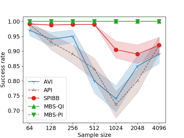
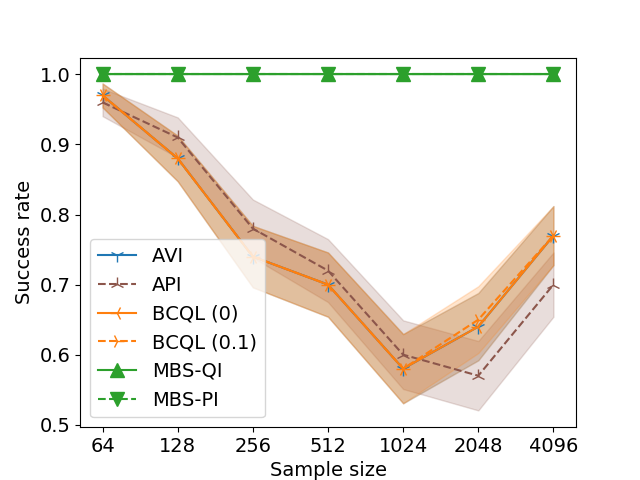
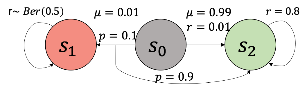
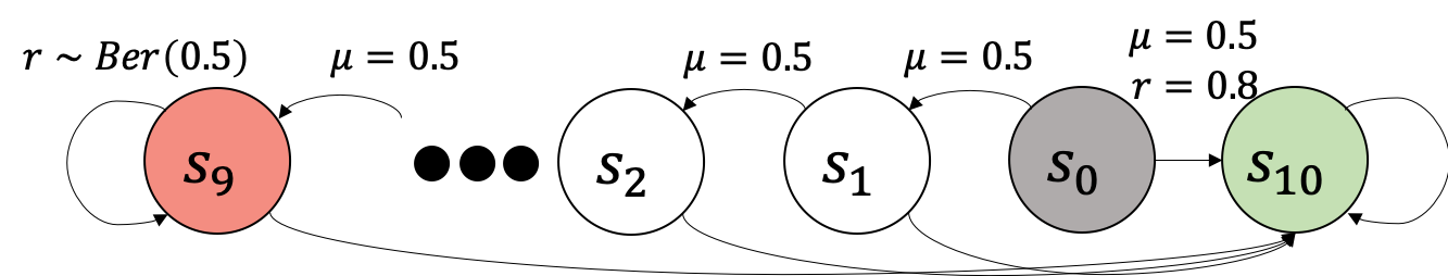
Nevertheless, the standard concentrability assumption has been employed in many prior works on API [20, 26] and AVI [27, 28, 10, 5]. In practice, these algorithms often divergeย [30, 13], likely due to the failure of this assumption. Such empirical observations have helped motivate several recent AVI (e.g.ย [11, 16]) and API (e.g.ย [19]) works that improve stability and performance. The BCQL algorithmย [11] only bootstraps value estimates from actions with conditional probabilities above a threshold under the behavior policy.111In their tabular algorithm BCQL the threshold is zero but we extend it to non-zero which is also more consistent with their deep RL variant BCQ. The BEAR algorithm [16] uses distribution-constrained backups as its prototype for theoretical analysis which, in the tabular setting, is essentially BCQL using non-zero threshold. SPIBBย [19] follows the behavior policy in less explored state-action pairs while attempting improvement everywhere else, assuming they know the behavior policy. However, we find that these algorithms have failure modes even in simple MDPs shown in Figureย 1. Specifically, BCQL and BEAR perform bootstrapping based on just the action probability, even if the state in question itself is less explored.222This corresponds to a small $f(\epsilon)$ in Theorem 4.2 of Kumar et al.ย [16], hence in line with their theory. This causes them to bootstrap values from infrequent states in the data, leading to bad performance as shown in Figureย 2. SPIBB is robust to this failure mode when the behavior policy is known. In this paper, we do not make this assumption as it is unknown in many settings (e.g., physiciansโ€™ decision making policy in a medical dataset). Consequently, following the estimated behavior policy from rare transitions is dangerous as our estimates can also be unreliable there. This can yield poor performance as shown in Figureย 2. In that plot, rare events start to appear as sample size increases and baseline algorithms begin to bootstrap unsafe values. Hence we see poor success rate as we get more behavior data. As samples size get very large all algorithms eventually see enough data to correct this effect. Next we describe the design and underlying theory for our new algorithms that successfully perform in these challenging MDPs (see Figureย 2).

4 Marginalized Behavior Supported Algorithms

Our aim is to create algorithms that are guaranteed to find an approximately optimal policy over all policies that only visit states and actions with sufficient visitation under $\mu$. In order to present the algorithms, we introduce some useful notation and present the classical fitted $Q$ iteration (FQI)ย [33] and fitted policy iteration (FPI)ย [3] algorithms which are the function approximation counterparts of AVI and API respectively. For the FPI algorithm, let ฮ โŠ‚(๐’ฎโ†’ฮ”โ€‹(๐’œ))ฮ โ†’๐’ฎฮ”๐’œ\Pi\subset(\mathcal{S}\to\Delta(\mathcal{A})) be a policy class. Let $\mathcal{F}\subseteq(\mathcal{S}\times\mathcal{A}\to[0,V_{\max}])$ be a $Q$ function class in both FQI and FPI. We assume ฮ ฮ \Pi and $\mathcal{F}$ are both finite but can be very large (error bounds will depend on logโก(|โ„ฑ|โ€‹|ฮ |)โ„ฑฮ \log(|\mathcal{F}||\Pi|)). For any function $g$ we define shorthand $\|g\|_{p,\mu}$ to denote (๐”ผ(s,a)โˆผฮผโกgโ€‹(s,a)p)1/psuperscriptsubscript๐”ผsimilar-to๐‘ ๐‘Ž๐œ‡๐‘”superscript๐‘ ๐‘Ž๐‘1๐‘(\operatorname{\mathbb{E}}_{(s,a)\sim\mu}g(s,a)^{p})^{1/p}. FQI updates $f_{k+1}=\operatorname*{arg\,min}_{f\in\mathcal{F}}\|f-\widehat{\mathcal{T}}f_{k}\|_{2,\mu}^{2}$ and returns the greedy policy with respect to the final $f_{k}$ upon termination. FPI instead iterates $f_{i+1}=\operatorname*{arg\,min}_{f\in\mathcal{F}}\|f-\widehat{\mathcal{T}}^{\pi_{k}}f_{i}\|_{2,\mu}^{2}$ until convergence to get $f_{k+1}$ followed by the greedy policy update to get $\pi_{k+1}$. When a restricted policy set ฮ ฮ \Pi is specified so that the greedy policy improvement is not possible, weighted classification is used to update the policy in some prior worksย [9]. Since both AVI and API suffer from bootstrapping errors in less visited regions of the MDP even in the tabular setting, FQI and FPI approaches have the same drawback.

We now show how to design more robust algorithms by constraining the Bellman update to be only over state action pairs that are sufficiently covered by $\mu$. Implementing such a constraint requires access to the density function $\mu$, over an extremely large or infinite space. Given we have samples of this distribution, several density estimation techniquesย [23, 24] can be used to estimate $\mu$ in practice, and here we assume we have a density function $\widehat{\mu}$ which is an approximate estimate of $\mu$. In the analysis section we will specify how our error bounds scale with the accuracy of $\widehat{\mu}$. Given $\widehat{\mu}$ and a threshold $b$ (as algorithm input) we define a filter function over the state-action space $\mathcal{S}\times\mathcal{A}$:

ฮถโ€‹(s,a;ฮผ^,b)=๐Ÿ™โ€‹(ฮผ^โ€‹(s,a)โ‰ฅb).๐œ๐‘ ๐‘Ž^๐œ‡๐‘1^๐œ‡๐‘ ๐‘Ž๐‘\zeta(s,a;\widehat{\mu},b)=\mathds{1}\left(\widehat{\mu}(s,a)\geq b\right). (1)

For simplicity we write ฮถโ€‹(s,a;ฮผ^,b)๐œ๐‘ ๐‘Ž^๐œ‡๐‘\zeta(s,a;\widehat{\mu},b) as ฮถโ€‹(s,a)๐œ๐‘ ๐‘Ž\zeta(s,a) and define ฮถโˆ˜fโ€‹(s,a):=ฮถโ€‹(s,a)โ€‹fโ€‹(s,a)assign๐œ๐‘“๐‘ ๐‘Ž๐œ๐‘ ๐‘Ž๐‘“๐‘ ๐‘Ž\zeta\circ f(s,a):=\zeta(s,a)f(s,a).

Algorithm 1 MBS Policy Iteration (MBS-PI) 1:Input: $D$, $\mathcal{F}$, ฮ ฮ \Pi, $\widehat{\mu}$, $b$ 2:Output: $\widehat{\pi}_{T}$ 3:forย t=0๐‘ก0t=0 to $T-1$ย do 4:ย ย ย ย ย forย k=0๐‘˜0k=0 to $K$ย do 5:ย ย ย ย ย ย ย ย ย ft,k+1โ†argโ€‹minfโˆˆโ„ฑโกโ„’Dโ€‹(f,ft,k;ฯ€^t)โ†subscript๐‘“๐‘ก๐‘˜1subscriptargmin๐‘“โ„ฑsubscriptโ„’๐ท๐‘“subscript๐‘“๐‘ก๐‘˜subscript^๐œ‹๐‘กf_{t,k+1}\!\leftarrow\!\operatorname*{arg\,min}_{f\in\mathcal{F}}\mathcal{L}_{D}(f,f_{t,k};\widehat{\pi}_{t}) 6:ย ย ย ย ย endย for 7:ย ย ย ย ย ฯ€^t+1โ†argโ€‹maxฯ€โˆˆฮ โก๐”ผDโ€‹[๐”ผฯ€โ€‹[ฮถโˆ˜ft,K+1]]โ†subscript^๐œ‹๐‘ก1subscriptargmax๐œ‹ฮ subscript๐”ผ๐ทdelimited-[]subscript๐”ผ๐œ‹delimited-[]๐œsubscript๐‘“๐‘ก๐พ1\widehat{\pi}_{t+1}\!\leftarrow\!\operatorname*{arg\,max}_{\pi\in\Pi}\mathbb{E}_{D}[\mathbb{E}_{\pi}\left[\zeta\circ f_{t,K+1}\right]] 8:endย for Algorithm 2 MBS $Q$ Iteration (MBS-QI) 1:Input: $D$, $\mathcal{F}$, $\widehat{\mu}$, $b$ 2:Output: $\widehat{\pi}_{T}$ 3:forย t=0๐‘ก0t=0 to $T-1$ย do 4:ย ย ย ย ย ft+1โ†argโ€‹minfโˆˆโ„ฑโกโ„’Dโ€‹(f;ft)โ†subscript๐‘“๐‘ก1subscriptargmin๐‘“โ„ฑsubscriptโ„’๐ท๐‘“subscript๐‘“๐‘กf_{t+1}\!\leftarrow\!\operatorname*{arg\,min}_{f\in\mathcal{F}}\mathcal{L}_{D}(f;f_{t}) 5:ย ย ย ย ย ฯ€^t+1โ€‹(s)โ†argโ€‹maxaโˆˆ๐’œโกฮถโˆ˜ft+1โ€‹(s,a)โ†subscript^๐œ‹๐‘ก1๐‘ subscriptargmax๐‘Ž๐’œ๐œsubscript๐‘“๐‘ก1๐‘ ๐‘Ž\widehat{\pi}_{t+1}(s)\!\!\leftarrow\!\!\operatorname*{arg\,max}_{a\in\mathcal{A}}\zeta\circ f_{t+1}(s,a) 6:endย for

We now introduce our Marginalized Behavior Supported Policy Iteration (MBS-PI) algorithm (Algorithmย 1), a minor modification to vanilla FPI that constrains the Bellman backups and policy improvement step to have sufficient support by the provided data. The key is to change the policy evaluation operator and only evaluate next step policy value over supported (s,a)๐‘ ๐‘Ž(s,a) pairs, and constrain policy improvement to only optimize over supported (s,a)๐‘ ๐‘Ž(s,a) pairs defined by $\zeta$. We define the $\zeta$-constrained Bellman evaluation operator $\widetilde{\mathcal{T}}^{\pi}$ as, for any $f:\mathcal{S}\times\mathcal{A}\to\mathbb{R}$,

(๐’ฏ~ฯ€โ€‹f)โ€‹(s,a)=rโ€‹(s,a)+ฮณโ€‹๐”ผsโ€ฒโ€‹โˆ‘aโ€ฒโˆˆ๐’œ[ฯ€โ€‹(aโ€ฒ|sโ€ฒ)โ€‹ฮถโˆ˜fโ€‹(sโ€ฒ,aโ€ฒ)].superscript~๐’ฏ๐œ‹๐‘“๐‘ ๐‘Ž๐‘Ÿ๐‘ ๐‘Ž๐›พsubscript๐”ผsuperscript๐‘ โ€ฒsubscriptsuperscript๐‘Žโ€ฒ๐’œdelimited-[]๐œ‹conditionalsuperscript๐‘Žโ€ฒsuperscript๐‘ โ€ฒ๐œ๐‘“superscript๐‘ โ€ฒsuperscript๐‘Žโ€ฒ\displaystyle(\widetilde{\mathcal{T}}^{\pi}f)(s,a)=r(s,a)+\gamma\mathbb{E}_{s^{\prime}}\textstyle\sum_{a^{\prime}\in\mathcal{A}}\left[\pi(a^{\prime}|s^{\prime})\zeta\circ f(s^{\prime},a^{\prime})\right]. (2)

This reduces updates that may be over-optimistic estimates in (sโ€ฒ,aโ€ฒ)superscript๐‘ โ€ฒsuperscript๐‘Žโ€ฒ(s^{\prime},a^{\prime})โ€™s that are not adequately covered by $\mu$ by using the most pessimistic estimate of 00 from such pairs. There is an important difference with SPIBBย [19], which still backs up $f$ values (but by estimated behavior probabilities) from such rarely visited state-action pairs: given limited data, this can lead to erroneous decisions (c.f. Fig.ย 2).

Given a batch dataset, we follow the common batch RL choice of least-squares residual minimizationย [26] and define empirical loss of $f$ given $f^{\prime}$ (from last iteration) and policy $\pi$:

โ„’Dโ€‹(f;fโ€ฒ,ฯ€):=๐”ผDโ€‹(fโ€‹(s,a)โˆ’rโˆ’ฮณโ€‹โˆ‘aโ€ฒโˆˆ๐’œฯ€โ€‹(aโ€ฒ|sโ€ฒ)โ€‹ฮถโˆ˜fโ€ฒโ€‹(sโ€ฒ,aโ€ฒ))2.assignsubscriptโ„’๐ท๐‘“superscript๐‘“โ€ฒ๐œ‹subscript๐”ผ๐ทsuperscript๐‘“๐‘ ๐‘Ž๐‘Ÿ๐›พsubscriptsuperscript๐‘Žโ€ฒ๐’œ๐œ‹conditionalsuperscript๐‘Žโ€ฒsuperscript๐‘ โ€ฒ๐œsuperscript๐‘“โ€ฒsuperscript๐‘ โ€ฒsuperscript๐‘Žโ€ฒ2\displaystyle\textstyle\mathcal{L}_{D}(f;f^{\prime},\pi):=\mathbb{E}_{D}\left(f(s,a)-r-\gamma\sum_{a^{\prime}\in\mathcal{A}}\pi(a^{\prime}|s^{\prime})\zeta\circ f^{\prime}(s^{\prime},a^{\prime})\right)^{2}.

In the policy improvement step (lineย 7 of Algorithmย 1), to ensure that the resulting policy has sufficient support, our algorithm applies the filter to the computed state-action values before performing maximization, like classification-based APIย [9]. We maximize using the dataset $D$ ($\operatorname{\mathbb{E}}_{D}$ is a sample average) and within the policy class ฮ ฮ \Pi, which may not include all deterministic policies.

Analogous to MBS-PI, we introduce Marginalized Behavior Supported $Q$ Iteration (MBS-QI) (Algorithmย 2) which constrains the Bellman backups to have sufficient support in the provided data. Define $\widetilde{\mathcal{T}}$ to be a $\zeta$-constrained Bellman optimality operator: for any $f:\mathcal{S}\times\mathcal{A}\to\mathbb{R}$,

(๐’ฏ~โ€‹f)โ€‹(s,a):=rโ€‹(s,a)+ฮณโ€‹๐”ผsโ€ฒโ€‹[maxaโ€ฒโกฮถโˆ˜fโ€‹(sโ€ฒ,aโ€ฒ)].assign~๐’ฏ๐‘“๐‘ ๐‘Ž๐‘Ÿ๐‘ ๐‘Ž๐›พsubscript๐”ผsuperscript๐‘ โ€ฒdelimited-[]subscriptsuperscript๐‘Žโ€ฒ๐œ๐‘“superscript๐‘ โ€ฒsuperscript๐‘Žโ€ฒ\displaystyle\textstyle(\widetilde{\mathcal{T}}f)(s,a):=r(s,a)+\gamma\mathbb{E}_{s^{\prime}}\left[\max_{a^{\prime}}\zeta\circ f(s^{\prime},a^{\prime})\right]. (3)

Similarly, we define the empirical loss of $f$ given another function $f^{\prime}$ as:

โ„’Dโ€‹(f;fโ€ฒ):=๐”ผDโ€‹(fโ€‹(s,a)โˆ’rโˆ’ฮณโ€‹maxaโ€ฒโˆˆ๐’œโกฮถโˆ˜fโ€ฒโ€‹(sโ€ฒ,aโ€ฒ))2.assignsubscriptโ„’๐ท๐‘“superscript๐‘“โ€ฒsubscript๐”ผ๐ทsuperscript๐‘“๐‘ ๐‘Ž๐‘Ÿ๐›พsubscriptsuperscript๐‘Žโ€ฒ๐’œ๐œsuperscript๐‘“โ€ฒsuperscript๐‘ โ€ฒsuperscript๐‘Žโ€ฒ2\displaystyle\textstyle\mathcal{L}_{D}(f;f^{\prime}):=\mathbb{E}_{D}\left(f(s,a)-r-\gamma\textstyle\max_{a^{\prime}\in\mathcal{A}}\zeta\circ f^{\prime}(s^{\prime},a^{\prime})\right)^{2}.

We also alter the final policy output step to only be able to select among actions which lie in the support set (lineย 5 of Algorithmย 2). In Figureย 2 we showed empirically that our MBS-QI and MBS-PI can both successfully return the optimal policy when the data distribution covers the optimal policy in two illustrative examples where prior approaches struggle. The threshold $b$ is the only hyper-parameter needed for our algorithms. Intuitively, $b$ trades off the risk of extrapolation with the potential benefits from more of the batch dataset. We discuss how practitioners can set $b$ in Sectionย 6.

5 Analysis

We now provide performance bounds on the policy output by MBS-PI and MBS-QI. Complete proofs for both are in the appendix.

5.1 Main results for MBS-PI

We start with some definitions and assumptions. Given $\pi$, let ฮทhฯ€โ€‹(s)subscriptsuperscript๐œ‚๐œ‹โ„Ž๐‘ \eta^{\pi}_{h}(s) be the marginal distribution of shsubscript๐‘ โ„Žs_{h} under $\pi$, that is, ฮทhฯ€โ€‹(s):=Prโก[sh=s|ฯ€]assignsubscriptsuperscript๐œ‚๐œ‹โ„Ž๐‘ Prsubscript๐‘ โ„Žconditional๐‘ ๐œ‹\eta^{\pi}_{h}(s):=\Pr[s_{h}=s|\pi], ฮทhฯ€โ€‹(s,a)=ฮทhฯ€โ€‹(s)โ€‹ฯ€โ€‹(a|s)subscriptsuperscript๐œ‚๐œ‹โ„Ž๐‘ ๐‘Žsubscriptsuperscript๐œ‚๐œ‹โ„Ž๐‘ ๐œ‹conditional๐‘Ž๐‘ \eta^{\pi}_{h}(s,a)=\eta^{\pi}_{h}(s)\pi(a|s), and ฮทฯ€โ€‹(s,a)=(1โˆ’ฮณ)โ€‹โˆ‘h=0โˆžฮณhโ€‹ฮทhฯ€โ€‹(s,a)superscript๐œ‚๐œ‹๐‘ ๐‘Ž1๐›พsuperscriptsubscriptโ„Ž0superscript๐›พโ„Žsubscriptsuperscript๐œ‚๐œ‹โ„Ž๐‘ ๐‘Ž\eta^{\pi}(s,a)=(1-\gamma)\sum_{h=0}^{\infty}\gamma^{h}\eta^{\pi}_{h}(s,a). We make the following assumptions:

Assumption 1 (Bounded densities).

For any non-stationary policy $\pi$ and $h\geq 0$, ฮทhฯ€โ€‹(s,a)โ‰คUsubscriptsuperscript๐œ‚๐œ‹โ„Ž๐‘ ๐‘Ž๐‘ˆ\eta^{\pi}_{h}(s,a)\leq U.

Assumption 2 (Density estimation error).

With probability at least $1-\delta$, $\|\widehat{\mu}-\mu\|_{\text{TV}}\leq\epsilon_{\mu}$.

Assumption 3 (Completeness under $\widetilde{\mathcal{T}}^{\pi}$).

โˆ€ฯ€โˆˆฮ for-all๐œ‹ฮ \forall\pi\in\Pi, $\max_{f\in\mathcal{F}}\min_{g\in\mathcal{F}}\|g-\widetilde{\mathcal{T}}^{\pi}f\|_{2,\mu}^{2}\leq\epsilon_{\mathcal{F}}.$

Assumption 4 (ฮ ฮ \Pi Completeness).

$\forall f\in\mathcal{F}$, minฯ€โˆˆฮ โกโ€–๐”ผฯ€โ€‹[ฮถโˆ˜fโ€‹(s,a)]โˆ’maxaโกฮถโˆ˜fโ€‹(s,a)โ€–1,ฮผโ‰คฯตฮ subscript๐œ‹ฮ subscriptnormsubscript๐”ผ๐œ‹delimited-[]๐œ๐‘“๐‘ ๐‘Žsubscript๐‘Ž๐œ๐‘“๐‘ ๐‘Ž1๐œ‡subscriptitalic-ฯตฮ \min_{\pi\in\Pi}\|\mathbb{E}_{\pi}\left[\zeta\circ f(s,a)\right]-\max_{a}\zeta\circ f(s,a)\|_{1,\mu}\leq\epsilon_{\Pi}.

Assumptions 3 and 4 are common but adapted to our $\zeta-$filtered operators, implying that the function class chosen is approximately complete with respect to our operator and that policy class can approximately recover the greedy policy. Assumptions 1 and 2 are novel. Assumption 2 bounds the accuracy of estimating the stateโ€“action behavior density function from limited data: $1/\sqrt{n}$ errors are standard using maximum likelihood estimation for instanceย [38], and the size of this error appears in the bounds. Finally Assumption 1 that the probability/density of any marginal state distribution is bounded is not very restrictive.333We need this assumption only because we filter based on $\hat{\mu}$ instead of $\eta^{\pi}/\mu$ during policy improvement. For example, this assumption holds when the density function of transitions $p(\cdot|s,a)$ and the initial state distribution are both bounded. This is always true for discrete spaces, and also holds for many distributions in continuous spaces including Gaussian distributions.

The dataset may not have sufficient samples of stateโ€“action pairs likely under the optimal policy in order to reliably and confidently return the optimal policy. Instead we hope and will show that our methods will return a policy that is close to the best policy which has sufficient support in the provided dataset. More formally, given a $\zeta$ filter over stateโ€“action pairs, we define a set of policies:

Definition 1 ($\zeta$-constrained policy setย ).

Let ฮ Caโ€‹lโ€‹lsuperscriptsubscriptฮ ๐ถ๐‘Ž๐‘™๐‘™\Pi_{C}^{all} be the set of policies $\mathcal{S}\to\Delta(\mathcal{A})$ such that Prโก(ฮถโ€‹(s,a)=0|ฯ€)โ‰คฯตฮถPr๐œ๐‘ ๐‘Žconditional0๐œ‹subscriptitalic-ฯต๐œ\Pr(\zeta(s,a)=0|\pi)\leq\epsilon_{\zeta}. That is, ๐”ผs,aโˆผฮทฯ€โ€‹[๐Ÿ™โ€‹(ฮถโ€‹(s,a)=0)]โ‰คฯตฮถsubscript๐”ผsimilar-to๐‘ ๐‘Žsuperscript๐œ‚๐œ‹delimited-[]1๐œ๐‘ ๐‘Ž0subscriptitalic-ฯต๐œ\mathbb{E}_{s,a\sim\eta^{\pi}}\left[\mathds{1}\left(\zeta(s,a)=0\right)\right]\leq\epsilon_{\zeta}.

$\epsilon_{\zeta}$ defines the probability under a policy of escaping to state-actions with insufficient data during an episode. ฮ Caโ€‹lโ€‹lsuperscriptsubscriptฮ ๐ถ๐‘Ž๐‘™๐‘™\Pi_{C}^{all} adapts its size w.r.t. the filter $\zeta$ which is a function of the hyper-parameter $b$, and ฮ Caโ€‹lโ€‹lsuperscriptsubscriptฮ ๐ถ๐‘Ž๐‘™๐‘™\Pi_{C}^{all} does not need to be contained in ฮ ฮ \Pi. We now lower bound the value of the policy returned by MBS-PI by the value of any ฯ€~โˆˆฮ Caโ€‹lโ€‹l~๐œ‹superscriptsubscriptฮ ๐ถ๐‘Ž๐‘™๐‘™\widetilde{\pi}\in\Pi_{C}^{all} up to a small error, which implies a small error w.r.t. the policy with the highest value in ฮ Caโ€‹lโ€‹lsuperscriptsubscriptฮ ๐ถ๐‘Ž๐‘™๐‘™\Pi_{C}^{all}. For ease of notation, we will denote $C=U/b$ in our results and analysis, being clear that $C$ is not assumed (as in concentrability) and is simply a function of the hyper-parameter $b$.

Theorem 1 (Comparison with best covered policy).

With Assumption 1 and 2 holds, given an MDP $M$, a dataset D={(s,a,r,sโ€ฒ)}๐ท๐‘ ๐‘Ž๐‘Ÿsuperscript๐‘ โ€ฒD=\{(s,a,r,s^{\prime})\} with $n$ samples drawn i.i.d. from $\mu\times R\times P$, and a Q-function class $\mathcal{F}$ and a policy class ฮ ฮ \Pi satisfying Assumption 3 and 4, $\widehat{\pi}_{t}$ from Algorithm 1 satisfies that w. p. at least $1-3\delta$,

vMฯ€~โˆ’vMฯ€^tโ‰ค๐’ชโ€‹(Cโ€‹Vmax2โ€‹lnโก(|โ„ฑ|โ€‹|ฮ |/ฮด)(1โˆ’ฮณ)3โ€‹n)+8โ€‹Cโ€‹ฯตโ„ฑ+6โ€‹Cโ€‹Vmaxโ€‹ฯตฮผ(1โˆ’ฮณ)3+2โ€‹Cโ€‹ฯตฮ +3โ€‹ฮณKโˆ’1โ€‹Vmax(1โˆ’ฮณ)2+Vmaxโ€‹ฯตฮถ1โˆ’ฮณ,subscriptsuperscript๐‘ฃ~๐œ‹๐‘€subscriptsuperscript๐‘ฃsubscript^๐œ‹๐‘ก๐‘€๐’ช๐ถsuperscriptsubscript๐‘‰2โ„ฑฮ ๐›ฟsuperscript1๐›พ3๐‘›8๐ถsubscriptitalic-ฯตโ„ฑ6๐ถsubscript๐‘‰subscriptitalic-ฯต๐œ‡superscript1๐›พ32๐ถsubscriptitalic-ฯตฮ 3superscript๐›พ๐พ1subscript๐‘‰superscript1๐›พ2subscript๐‘‰subscriptitalic-ฯต๐œ1๐›พ\displaystyle v^{\widetilde{\pi}}_{M}-v^{\widehat{\pi}_{t}}_{M}\leq\mathcal{O}\left(\frac{C\sqrt{V_{\max}^{2}\ln(|\mathcal{F}||\Pi|/\delta)}}{(1-\gamma)^{3}\sqrt{n}}\right)+\frac{8C\sqrt{\epsilon_{\mathcal{F}}}+6CV_{\max}\epsilon_{\mu}}{(1-\gamma)^{3}}+\frac{2C\epsilon_{\Pi}+3\gamma^{K-1}V_{\max}}{(1-\gamma)^{2}}+\frac{V_{\max}\epsilon_{\zeta}}{1-\gamma},

for any policy ฯ€~โˆˆฮ Caโ€‹lโ€‹l~๐œ‹superscriptsubscriptฮ ๐ถ๐‘Ž๐‘™๐‘™\widetilde{\pi}\in\Pi_{C}^{all} under Assumptionsย 1 andย 2 and any $t\geq K$. $C=U/b$. $K$ is the number of policy evaluation iterations (inner loop) and $t$ is the number of policy improvement steps.

Proof sketch. The key is to characterize the filtration effect of the conservative Bellman operators in terms of the resulting value function estimates. As an analysis tool, we construct an auxiliary MDP $M^{\prime}$ by adding one additional action $a_{\text{abs}}$ in each state, leading to a zero reward absorbing state sabssubscript๐‘ abss_{\text{abs}}. For a subset of policies in $M^{\prime}$, the fixed point of our conservative operator $\widetilde{\mathcal{T}}^{\pi}$ is $Q^{\pi}$ in $M^{\prime}$. For that subset, we also have a bounded density ratio, thus we can provide the error bound in $M^{\prime}$. For any $\zeta$-constrained policy, we show that it can be mapped to that subset of policies in $M^{\prime}$ without much loss of value, and then we finish the proof to yield a bound in $M$. โˆŽ

Our results match in $n$ the fast rate error bound of API/AVI [7, 29, 5, 20]. The dependency on horizon also matches the standard API analysis and is $\mathcal{O}(1/(1-\gamma)^{3})$. The dependency on $U/b$ is same as the dependency on concentrability coefficient for vanilla API analysis, but our guarantee adapts given a hyper-parameter choice instead of imposing a worst case bound over all policies. Unlike Theorem 4.2 of Kumar et al.ย [16], there is no uncontrolled $f(\epsilon)$-like term. We avoid that term by placing stronger restrictions in our updates and in the comparator class ฮ Caโ€‹lโ€‹lsuperscriptsubscriptฮ ๐ถ๐‘Ž๐‘™๐‘™\Pi_{C}^{all}: note that if Kumar et al. were to use our comparator class ฮ Caโ€‹lโ€‹lsuperscriptsubscriptฮ ๐ถ๐‘Ž๐‘™๐‘™\Pi_{C}^{all}, they would not recover our guarantees (see also discussion of BEAR in Sectionย 3). When there is an optimal policy with small escaping probability from support of $\zeta$, we obtain an error bound relative to the optimal value.

Corollary 1 ($\mu$ covers an optimal policy).

If there exists an optimal policy $\pi^{\star}$ in $M$ such that Prโก(ฮผโ€‹(s,a)โ‰ค2โ€‹b|ฯ€โ‹†)โ‰คฯตPr๐œ‡๐‘ ๐‘Žconditional2๐‘superscript๐œ‹โ‹†italic-ฯต\Pr(\mu(s,a)\leq 2b|\pi^{\star})\leq\epsilon. then under the conditions in Theorem 1, $\widehat{\pi}_{t}$ returned by Algorithm 1 satisfies that with probability at least $1-3\delta$, $v^{\widehat{\pi}_{t}}_{M}\geq v^{\star}_{M}-\Delta$, where $\Delta$ is the right hand side of Theorem 1 and $\epsilon_{\zeta}$ in $\Delta$ is $\epsilon+C\epsilon_{\mu}$.

When the completeness assumptions holds without error and $\gamma^{K-1}\leq\epsilon$, the error bound reduces to

vMฯ€^tโ‰ฅvMโ‹†โˆ’๐’ชโ€‹(Cโ€‹lnโก(|โ„ฑ|โ€‹|ฮ |/ฮด)/n+Cโ€‹ฯตฮผ+ฯต)โ€‹Vmax/(1โˆ’ฮณ)3subscriptsuperscript๐‘ฃsubscript^๐œ‹๐‘ก๐‘€subscriptsuperscript๐‘ฃโ‹†๐‘€๐’ช๐ถโ„ฑฮ ๐›ฟ๐‘›๐ถsubscriptitalic-ฯต๐œ‡italic-ฯตsubscript๐‘‰superscript1๐›พ3\displaystyle v^{\widehat{\pi}_{t}}_{M}\geq v^{\star}_{M}-\mathcal{O}\left(C\sqrt{\ln(|\mathcal{F}||\Pi|/\delta)/n}+C\epsilon_{\mu}+\epsilon\right)V_{\max}/(1-\gamma)^{3}

This is similarly tight as prior analysis assuming concentrabilityย [17, 4]. For MBS-QI, the error bound is in a similar form. However the general MBS-QI bound of Corollaryย 3 has an additional Bellman residual term related to $\widetilde{\mathcal{T}}$ and $\pi^{\star}$. This term arises since in value iteration, the fixed point of $\widetilde{\mathcal{T}}$ may no longer be the value function of the optimal policy under support. When comparing to on-policy policy optimizationย [14, 31, 2, 12], the constant $C$ is akin to the density ratio with respect to an optimal policy in those works, though we pay an additional price on the size of densities. The terms regarding value function completeness can be avoided by Monte-carlo estimation in on-policy settings and there is no need for density estimation to regularize value bootstrapping either.

Note that if we can find a $b$ and $\epsilon_{\zeta}$ such that ฮผโˆˆฮ Caโ€‹lโ€‹l๐œ‡superscriptsubscriptฮ ๐ถ๐‘Ž๐‘™๐‘™\mu\in\Pi_{C}^{all} given sufficient data, then Theoremย 1 immediately yields a policy improvement guarantee too, analogous to the tabular guarantees known for BCQL, SPIBB and other safe policy improvement guarantees. Here, we provide the safe policy improvement guarantees in tabular settings. The details of proof are in Appendix C.5.

Corollary 2 (Safe policy improvement โ€“ discrete state space).

For finite state action spaces and $b\leq\mu_{\min}$, under the same assumptions as Theorem 1, there exist function sets $\mathcal{F}$ and ฮ ฮ \Pi (specified in the proof) such that $\widehat{\pi}_{t}$ from Algorithm 1 satisfies that with probability at least $1-3\delta$,

$\displaystyle v^{\hat{\pi}_{t}}_{M}\geq v^{\mu}_{M}-\widetilde{\mathcal{O}}\left(\frac{V_{\max}}{b(1-\gamma)^{3}}\left(\frac{|\mathcal{S}||\mathcal{A}|}{n}+\sqrt{\frac{|\mathcal{S}||\mathcal{A}|}{n}}\right)+\frac{\gamma^{K}V_{\max}}{(1-\gamma)^{2}}\right)$

This corollary is comparable with the safe policy improvement result in [19] in its $\mathcal{S}$, $\mathcal{A}$ dependence. Note that their hyper-parameter $N_{\land}$ is analogous to $bn$ in our result. Our dependency on $1-\gamma$ is worse, as our algorithm is not designed for the tabular setting, and matches prior results in the function approximation setting as remarked after Theoremย 1.

5.2 Main results for MBS-VI

Now we show the error bound of our value iteration algorithm, MBS-QI. First we introduce a similar completeness assumption about the Bellman optimality operator:

Assumption 5 (Completeness under $\widetilde{\mathcal{T}}$).

$\max_{f\in\mathcal{F}}\min_{g\in\mathcal{F}}\|g-\widetilde{\mathcal{T}}f\|_{2,\mu}^{2}\leq\epsilon^{\prime}_{\mathcal{F}}$

The main theorem for value iteration is similar with the policy iteration error bound

Theorem 2.

Under Assumption 1 and 2, given a MDP $M=<\mathcal{S},\mathcal{A},R,P,\gamma,p>$, a dataset D={(s,a,r,sโ€ฒ)}๐ท๐‘ ๐‘Ž๐‘Ÿsuperscript๐‘ โ€ฒD=\{(s,a,r,s^{\prime})\} with $n$ samples that is draw i.i.d. from $\mu\times R\times P$, and a finite Q-function classes $\mathcal{F}$ satisfying Assumption 5, $\widehat{\pi}_{t}$ from Algorithm 2 satisfies that with probability at least $1-\delta$,

$\displaystyle v^{\widetilde{\pi}}-v^{\widehat{\pi}_{t}}\leq\frac{2C\left(\mathcal{O}\left(\sqrt{\frac{V_{\max}^{2}\ln(|\mathcal{F}|/\delta)}{n}}\right)+\sqrt{\epsilon^{\prime}_{\mathcal{F}}}+V_{\max}\epsilon_{\mu}+\left\|Q^{\widetilde{\pi}}-\widetilde{\mathcal{T}}Q^{\widetilde{\pi}}\right\|_{2,\mu}\right)}{(1-\gamma)^{2}}+\frac{(2\gamma^{t}+\epsilon_{\zeta})V_{\max}}{1-\gamma}$

for any policy ฯ€~โˆˆฮ Caโ€‹lโ€‹l~๐œ‹superscriptsubscriptฮ ๐ถ๐‘Ž๐‘™๐‘™\widetilde{\pi}\in\Pi_{C}^{all}.

The error bound has similar dependency on $C$, $\epsilon^{\prime}_{\mathcal{F}}$, $n$ as in the API case. The dependency on horizon is $\mathcal{O}(1/(1-\gamma)^{2})$ which is standard in approximate value iteration analysis [27, 28]. The term $\|\zeta(Q^{\Xi(\widetilde{\pi})}-\widetilde{\mathcal{T}}Q^{\Xi(\widetilde{\pi})})\|_{2,\mu}$ in the error bound in Theorem 2 comes from the fact that the bound applies to any policy $\widetilde{\pi}$ in the $\zeta$-constrained policy setย , which might not be optimal. The scale of this term approximately measures the sub-optimality of the policy $\widetilde{\pi}$. $\zeta$ implies that we only measure the sub-optimality in state-action pairs visited often enough in the data. By choosing the best $\widetilde{\pi}$ in ฮ Caโ€‹lโ€‹lsuperscriptsubscriptฮ ๐ถ๐‘Ž๐‘™๐‘™\Pi_{C}^{all} with a good enough $Q^{\widetilde{\pi}}$ that term should be relatively small, and intuitively it measures โ€œhow good is the best policy with sufficient coverageโ€. This term is not universally guaranteed to be small, but empirically it can often be negligible, as our illustrative examples in Sectionย 3 demonstrate. In Appendixย D we develop a stronger notion of a constrained policy set such that, if $\pi^{*}$ is in that set then this error term is guaranteed to be small. Similar to Corollary 1, the same type of bound w.r.t. optimal policy can be derived, formally shown in Corollary 3.

Corollary 3.

If there exists an $\pi^{\star}$ on $M$ such that Prโก(ฮผโ€‹(s,a)โ‰ค2โ€‹b|ฯ€โ‹†)โ‰คฯตPr๐œ‡๐‘ ๐‘Žconditional2๐‘superscript๐œ‹โ‹†italic-ฯต\Pr(\mu(s,a)\leq 2b|\pi^{\star})\leq\epsilon. then under the condition as Theorem 2, $\widehat{\pi}_{t}$ from Algorithm 2 satisfies that with probability at least $1-2\delta$, $v^{\widehat{\pi}_{t}}_{M}\geq v^{\star}_{M}-\Delta$, where $\Delta$ is the right hand side of Theorem 2 and $\epsilon_{\zeta}$ in $\Delta$ is $\epsilon+C\epsilon_{\mu}$.

To summarize, our analysis makes two main contributions. First, compared to prior work which provides guarantees of the performance relative to the optimal policy under concentrability, we provide similar bounds by only requiring that an optimal policy, instead of every policy, is well supported by $\mu$. Second, when an optimal policy is not well supported, our algorithms are guaranteed to output a policy whose performance is near optimal in the supported policy class.

6 Experimental Results

The key innovation in our algorithm uses an estimated $\zeta$ to filter backups from unsound state-action pairs. In Section ย 3 we showed how prior approaches without this can fail in some illustrative examples. We now experiment in two standard domains โ€“ Cartpole and Mujoco, that utilize very different $\zeta$-estimation procedures. We show several experiments where the data collected ranges from being inadequate for batch RL to complete coverage (where even unsafe batch RL algorithms can succeed). Our algorithms return policies better than any baseline batch RL algorithm across the entire spectrum of datasets. Our algorithms need the hyperparameter $b$ to trade off conservatism of a large $b$ (where the algorithm stays at its initialization in the limit) and unfounded optimism of $b=0$ (classical FQI/FPI). In discrete spaces, we can set $b=n_{0}/n$ where $n_{0}$ is our prior for the number of samples we need for reliable distribution estimates and $n$ is the total sample size. In continuous spaces, we can set the threshold to be a percentile of $\widehat{\mu}$, so as to filter out updates from rare outliers in the dataset. We can also run post-hoc diagnostics on the choice of $b$ by computing the average of ฮถโ€‹(s,ฯ€โ€‹(s))๐œ๐‘ ๐œ‹๐‘ \zeta(s,\pi(s)) for the resulting policy $\pi$ over the batch dataset. If this quantity is too small, we can conclude that $\zeta$ filters out too many Bellman backups and hence rerun the procedure with a lower $b$.

6.1 MBS-QI in discrete spaces

We first compare MBS-QI with FQI, BCQL [11], SPIBB [19] and behavior cloning (BC) in OpenAI gym CartPole-v0, with a discrete state space by binning each state dimension resulting in $10000$ states. FQI uses a vanilla Bellman operator to update the $Q$ function in each iteration. For BCQL, we fit a modified operator in their Eq (10), changing the constraint ฮผ^โ€‹(a|s)>0^๐œ‡conditional๐‘Ž๐‘ 0\widehat{\mu}(a|s)>0 to allow a threshold $b\geq 0$. For SPIBB, we learn the $Q$ function by fitting the operator in their Eq (9) (SPIBB-DQN objective). Both SPIBB and MBS-QI require ฮผ^โ€‹(s,a)^๐œ‡๐‘ ๐‘Ž\widehat{\mu}(s,a) to construct the modified operator, but use different notions for being conservative. For all algorithms, ฮผ^โ€‹(s,a)^๐œ‡๐‘ ๐‘Ž\widehat{\mu}(s,a) and ฮผ^โ€‹(a|s)^๐œ‡conditional๐‘Ž๐‘ \widehat{\mu}(a|s) are constructed using empirical counts.
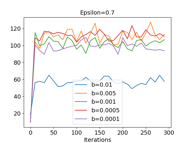
Refer to caption
Figure 3: CartPole-v0. Left: convergent policy value across different ($\epsilon$-greedy) behavior policies. Middle and Right: learning curves when $\epsilon=0.3,0.6$. We allow non-zero threshold for BCQL to subsume the tabular algorithm of BEARย [16].

We collect $n=10^{4}$ transitions from an epsilon-greedy policy w.r.t a near-optimal $Q$ function. We report the final policy value from different algorithms for epsilon from $0.1$ to $0.9$ in Figure 3 (left), and learning curves for $\epsilon=0.3,0.6$ in Figure 3 (middle, right). The results are averaged over 10 random seeds. Notice that BCQL, SPIBB, and our algorithm need a threshold of ฮผโ€‹(s,a)๐œ‡๐‘ ๐‘Ž\mu(s,a) or ฮผโ€‹(a|s)๐œ‡conditional๐‘Ž๐‘ \mu(a|s) as hyper-parameter. We show the results with the best threshold from $\{0.005,0.001,0.0001\}$ for ฮผโ€‹(s,a)๐œ‡๐‘ ๐‘Ž\mu(s,a) (MBS-QI, SPIBB) and $\{0,0.1\}$ for ฮผโ€‹(a|s)๐œ‡conditional๐‘Ž๐‘ \mu(a|s). Our algorithm picks larger $b$ for smaller $\epsilon$ which matches the intuition of more conservatism when the batch dataset is not sufficiently diverse. The results show that our algorithm achieves good performance among all different $\epsilon$ values, and is always better than both behavior cloning and vanilla FQI unlike other baselines.

6.2 MBS-QL in continuous spaces

The core argument for MBS is that $\zeta$-filtration should focus on state-action ฮผ^โ€‹(s,a)^๐œ‡๐‘ ๐‘Ž\widehat{\mu}(s,a) distributions rather than ฮผ^โ€‹(a|s)^๐œ‡conditional๐‘Ž๐‘ \widehat{\mu}(a|s). To test this argument in a more complex domain, we introduce MBS Q Learning (MBS-QL) for continuous action spaces which incorporates our $\zeta$-filtration on top of the BCQ architecture [11]. MBS-QL (like BCQ) employs an actor in continuous action space and a variational auto-encoder (VAE) to approximate ฮผโ€‹(a|s)๐œ‡conditional๐‘Ž๐‘ \mu(a|s). We use an additional VAE to fit the marginal state distribution in the dataset. Since the BCQ architecture already prevents backup from (s,a)๐‘ ๐‘Ž(s,a) with small ฮผโ€‹(a|s)๐œ‡conditional๐‘Ž๐‘ \mu(a|s), we construct an additional filter function ฮถโ€‹(s)๐œ๐‘ \zeta(s) on state space by ฮถโ€‹(s)=๐Ÿ™โ€‹(Eโ€‹Lโ€‹Bโ€‹Oโ€‹(s)>P2)๐œ๐‘ 1๐ธ๐ฟ๐ต๐‘‚๐‘ subscript๐‘ƒ2\zeta(s)=\mathds{1}(ELBO(s)>P_{2}) where Eโ€‹Lโ€‹Bโ€‹Oโ€‹(s)๐ธ๐ฟ๐ต๐‘‚๐‘ ELBO(s) is the evidence lower bound optimized by VAE, and $P_{2}$ is the $2^{nd}$ percentile of ELBO values of s๐‘ s in the whole batch. Thus the only difference between MBS-QL and BCQ is that MBS-QL applies additional filtration ฮถโ€‹(sโ€ฒ)๐œsuperscript๐‘ โ€ฒ\zeta(s^{\prime}) to the update from sโ€ฒsuperscript๐‘ โ€ฒs^{\prime} in Eq (13) in [11].

Refer to caption
Figure 4: MuJoCo Hopper-v3 domain. Averaged over 5 random seeds and the shadow region in plot shows the standard deviation.

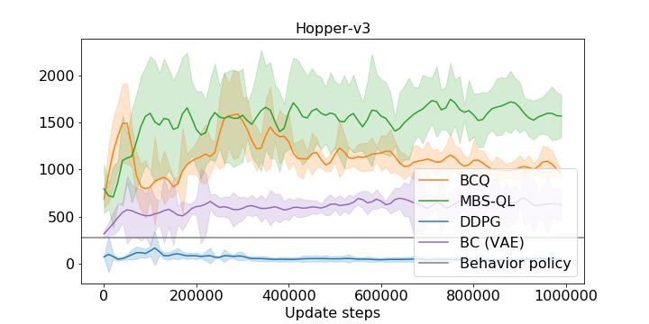
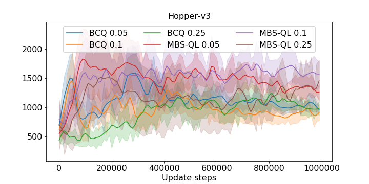
We compared MBS-QL, BCQ, DDPG, and behavior cloning in the Hopper-v3 domain in MuJoCo. DDPG is run with pure offline data to demonstrate the performance of a vanilla RL algorithm without adapting to the batch RL setting. Behavior cloning uses the same VAE to fit the behavior policy as MBS-QL and BCQ, and returns the learned behavior policy. The batch has $n=10^{5}$ transitions, and we use the same data collection policy as the โ€œImperfectโ€ batch in BCQย [11]; a near-optimal policy with two levels of noise: with probability $0.3$ it samples uniformly from action space, with probability $0.7$ it adds a Gaussian noise $\mathcal{N}(0,0.3)$ to the greedy action. In Figure 4, BCQ is able to achieve good policy beyond both vanilla DDPG and behavior cloning method, but can not maintain this improvement as it updates its Q function in an unsafe manner. This experiment demonstrates that the additional state support filter can prevent the collapse of BCQ.

7 Related Work

Research in batch RL focuses on deriving the best possible policy from the available dataย [18]. For practical settings that necessitate using function approximators, fitted value iterationย [6, 30] and fitted policy iterationย [17] provide an empirical foundation that has spawned many successful modern deep RL algorithms. Many prior works provide error bounds as a function of the violation of realizability and completeness assumptions such asย [36]. In the online RL setting, concentrability can be side-steppedย [37] but can still pose a significant challenge (e.g., the hardness of exploration inย [5]). A commonly-used equivalent form of the concentrability assumption is on the discounted summation of ratios between the product of probabilities over state actions under any policy, to the data generating distributionย [3, 21]. Our goal is to relax such assumptions to make the resulting algorithms more practically useful.

Several heuristics [13, 30, 11] show that algorithmic modifications help alleviate the extrapolation error or maximization bias empirically. This paper provides a simple modification that has strong theoretical guarantees even with function approximation. In contrast, the theoretical results of BEAR [16] (Theorem 4.1 and 4.2) rely on a finite state space, while the algorithm analyzed in the proof is actually the same as BCQL with a non-zero threshold whose weakness is shown in Sections 3 and 6.1. Error bound in Theorem 4.1 of [16] has an additional non-diminishing term ฮฑโ€‹(ฮ )๐›ผฮ \alpha(\Pi), while non-diminishing terms in our Theorem 1 are the same as in standard analysis. Another recent work [2] highlights that sufficiently large and diverse datasets can lead to good batch RL results but we focus on the other side of the coin: a robust update rule even if we do not have a good dataset.

8 Discussion & Conclusion

We study a key assumption for analysis in batch value-based RL, concentrability, and provide policy iteration and $Q$ iteration algorithms with minor modifications that can be agnostic to this assumption. We remark that the other non-standard assumption about bounded density can be relaxed if we could construct the $\zeta$ filter by thresholding density ratios directly, but this results in a different filter for each policy encountered during the algorithmโ€™s operation. Being able to threshold density ratios will also allow us to assert that ฮผโˆˆฮ Caโ€‹lโ€‹l๐œ‡superscriptsubscriptฮ ๐ถ๐‘Ž๐‘™๐‘™\mu\in\Pi_{C}^{all} always, yielding imitation and policy improvement guarantees. We anticipate future work that develops batch RL algorithms that exploit this insight.

9 Broader Impact

Our improvements to batch RL may improve sample efficiency of online RL and safety of off-policy RL enough to consider them in some real-world applications. However we caution that more work is needed (e.g., in closely related areas of off-policy evaluation OPE, confidence estimation, interpretability etc.) before these methods can be reliably deployed in practice. For instance (see Figureย 4) no batch RL algorithm has (a) low variability across runs, (b) reliably terminates when discovering a good policy, (c) gives a sharp confidence interval of expected performance. We anticipate future work in batch RL and OPE that addresses these shortcomings.

References

  • [1] Alekh Agarwal, Shamย M Kakade, Jasonย D Lee, and Gaurav Mahajan. Optimality and approximation with policy gradient methods in markov decision processes. arXiv preprint arXiv:1908.00261, 2019.
  • [2] Rishabh Agarwal, Dale Schuurmans, and Mohammad Norouzi. An optimistic perspective on offline reinforcement learning. In ICML, 2020.
  • [3] Andrรกs Antos, Csaba Szepesvรกri, and Rรฉmi Munos. Learning near-optimal policies with bellman-residual minimization based fitted policy iteration and a single sample path. Machine Learning, 71:89โ€“129, 2008.
  • [4] Dimitriย P Bertsekas. Approximate policy iteration: A survey and some new methods. Journal of Control Theory and Applications, 9:310โ€“335, 2011.
  • [5] Jinglin Chen and Nan Jiang. Information-theoretic considerations in batch reinforcement learning. In ICML, pages 1042โ€“1051, 2019.
  • [6] Damien Ernst, Pierre Geurts, and Louis Wehenkel. Tree-based batch mode reinforcement learning. Journal of Machine Learning Research, 6:503โ€“556, 2005.
  • [7] Amir-massoud Farahmand. Regularization in reinforcement learning. PhD thesis, University of Alberta, 2011.
  • [8] Amir-massoud Farahmand, Mohammad Ghavamzadeh, Csaba Szepesvรกri, and Shie Mannor. Regularized policy iteration with nonparametric function spaces. The Journal of Machine Learning Research, 17:4809โ€“4874, 2016.
  • [9] Amir-massoud Farahmand, Doina Precup, Andrรฉย MS Barreto, and Mohammad Ghavamzadeh. Classification-based approximate policy iteration. IEEE Transactions on Automatic Control, 60:2989โ€“2993, 2015.
  • [10] Amir-massoud Farahmand, Csaba Szepesvรกri, and Rรฉmi Munos. Error propagation for approximate policy and value iteration. In NeurIPS, pages 568โ€“576, 2010.
  • [11] Scott Fujimoto, David Meger, and Doina Precup. Off-policy deep reinforcement learning without exploration. In ICML, pages 2052โ€“2062, 2019.
  • [12] Matthieu Geist, Bruno Scherrer, and Olivier Pietquin. A theory of regularized markov decision processes. arXiv preprint arXiv:1901.11275, 2019.
  • [13] Roland Hafner and Martin Riedmiller. Reinforcement learning in feedback control. Machine learning, 84:137โ€“169, 2011.
  • [14] Sham Kakade and John Langford. Approximately optimal approximate reinforcement learning. In ICML, pages 267โ€“274, 2002.
  • [15] Shamย M Kakade. A natural policy gradient. In NeurIPS, pages 1531โ€“1538, 2002.
  • [16] Aviral Kumar, Justin Fu, Matthew Soh, George Tucker, and Sergey Levine. Stabilizing off-policy q-learning via bootstrapping error reduction. In NeurIPS, pages 11761โ€“11771, 2019.
  • [17] Michailย G Lagoudakis and Ronald Parr. Least-squares policy iteration. Journal of machine learning research, 4:1107โ€“1149, 2003.
  • [18] Sascha Lange, Thomas Gabel, and Martin Riedmiller. Batch reinforcement learning. In Reinforcement learning, pages 45โ€“73. Springer, 2012.
  • [19] Romain Laroche, Paul Trichelair, and Remiย Tachet Desย Combes. Safe policy improvement with baseline bootstrapping. In ICML, pages 3652โ€“3661, 2019.
  • [20] Alessandro Lazaric, Mohammad Ghavamzadeh, and Rรฉmi Munos. Finite-sample analysis of least-squares policy iteration. Journal of Machine Learning Research, 13:3041โ€“3074, 2012.
  • [21] Hoang Le, Cameron Voloshin, and Yisong Yue. Batch policy learning under constraints. In ICML, pages 3703โ€“3712, 2019.
  • [22] Long-Ji Lin. Self-improving reactive agents based on reinforcement learning, planning and teaching. Machine learning, 8:293โ€“321, 1992.
  • [23] Cliveย R Loader etย al. Local likelihood density estimation. The Annals of Statistics, 24:1602โ€“1618, 1996.
  • [24] Peter Malec and Melanie Schienle. Nonparametric kernel density estimation near the boundary. Computational Statistics & Data Analysis, 72:57โ€“76, 2014.
  • [25] Volodymyr Mnih, Koray Kavukcuoglu, David Silver, Andreiย A Rusu, Joel Veness, Marcย G Bellemare, Alex Graves, Martin Riedmiller, Andreasย K Fidjeland, Georg Ostrovski, etย al. Human-level control through deep reinforcement learning. Nature, 518(7540):529โ€“533, 2015.
  • [26] Rรฉmi Munos. Error bounds for approximate policy iteration. In ICML, pages 560โ€“567, 2003.
  • [27] Rรฉmi Munos. Error bounds for approximate value iteration. In Proceedings of the National Conference on Artificial Intelligence, page 1006, 2005.
  • [28] Rรฉmi Munos and Csaba Szepesvรกri. Finite-time bounds for fitted value iteration. Journal of Machine Learning Research, 9:815โ€“857, 2008.
  • [29] Bernardoย Avila Pires and Csaba Szepesvรกri. Statistical linear estimation with penalized estimators: an application to reinforcement learning. arXiv preprint arXiv:1206.6444, 2012.
  • [30] Martin Riedmiller. Neural fitted q iterationโ€“first experiences with a data efficient neural reinforcement learning method. In European Conference on Machine Learning, pages 317โ€“328, 2005.
  • [31] Bruno Scherrer. Approximate policy iteration schemes: a comparison. In ICML, pages 1314โ€“1322, 2014.
  • [32] Richardย S Sutton and Andrewย G Barto. Reinforcement learning: An introduction. MIT press, 2018.
  • [33] Csaba Szepesvรกri and Rรฉmi Munos. Finite time bounds for sampling based fitted value iteration. In ICML, pages 880โ€“887, 2005.
  • [34] Philip Thomas, Georgios Theocharous, and Mohammad Ghavamzadeh. High Confidence Policy Improvement. In ICML, pages 2380โ€“2388, 2015.
  • [35] Philipย S Thomas, Brunoย Castro daย Silva, Andrewย G Barto, Stephen Giguere, Yuriy Brun, and Emma Brunskill. Preventing undesirable behavior of intelligent machines. Science, 366:999โ€“1004, 2019.
  • [36] Tengyang Xie and Nan Jiang. $q^{\star}$ approximation schemes for batch reinforcement learning: A theoretical comparison. UAI, 2020.
  • [37] Ming Yu, Zhuoran Yang, Mengdi Wang, and Zhaoran Wang. Provable q-iteration with l infinity guarantees and function approximation. Workshop on Optimization and RL, NeurIPS, 2019.
  • [38] Tong Zhang etย al. From epsilon-entropy to kl-entropy: Analysis of minimum information complexity density estimation. The Annals of Statistics, 34:2180โ€“2210, 2006.

In Appendix A we introduce some basic definitions that are needed for our theoretical results. In Appendix B, we provide a sufficient conditions for Assumption 1 that were mentioned in the main text. In Appendix C and Appendix D we prove the error bounds for MBS-PI and MBS-QI. In Appendix E and Appendix F we present more details of our experimental results.

Appendix A Definition of auxiliary MDP and policy projection

First we introduce the definition of an auxiliary MDP $M^{\prime}$ based on M: each state in M has an absorbing action which leads to a self-looping absorbing state. All the other dynamics are preserved. Rewards are 0 for the absorbing action and unchanged elsewhere. More formally: The auxiliary MDP $M^{\prime}$ given $M=<\mathcal{S},\mathcal{A},R,P,\gamma,\rho>$ is defined as $M^{\prime}=<\mathcal{S}^{\prime},\mathcal{A}^{\prime},R^{\prime},P^{\prime},\gamma,\rho>$, where ๐’ฎโ€ฒ=๐’ฎโ€‹โ‹ƒ{sabs}superscript๐’ฎโ€ฒ๐’ฎsubscript๐‘ abs\mathcal{S}^{\prime}=\mathcal{S}\bigcup\{s_{\text{abs}}\}, $\mathcal{A}^{\prime}=\mathcal{A}\bigcup\{a_{\text{abs}}\}$. $R^{\prime}$ and $P^{\prime}$ are the same as $R$ and $P$ for all (s,a)โˆˆ๐’ฎร—๐’œ๐‘ ๐‘Ž๐’ฎ๐’œ(s,a)\in\mathcal{S}\times\mathcal{A}. Rโ€ฒโ€‹(s,a)superscript๐‘…โ€ฒ๐‘ ๐‘ŽR^{\prime}(s,a) if s=sabs๐‘ subscript๐‘ abss=s_{\text{abs}} or $a=a_{\text{abs}}$ is a point mass on 00, and Pโ€ฒโ€‹(s,a)superscript๐‘ƒโ€ฒ๐‘ ๐‘ŽP^{\prime}(s,a) if s=sabs๐‘ subscript๐‘ abss=s_{\text{abs}} or $a=a_{\text{abs}}$ is a point mass on sabssubscript๐‘ abss_{\text{abs}}. A data set $D$ generated from distribution $\mu$ on $M$ is also from the distribution $\mu$ on $M^{\prime}$, since all distributions on $\mathcal{S}\times\mathcal{A}$ are the same between the two MDPs. This MDP is used only to perform our analysis about the error bounds on the algorithm, and is not needed at all for executing Algorithm 1 and 2. As some of the notations is actually a function of the MDP, we clarify the usage of notation w.r.t. $M$/$M^{\prime}$ in the appendix:

  1. 1.

    Policy value functions $V^{\pi}$/$Q^{\pi}$ and Bellman operators $\mathcal{T}$/$\mathcal{T}^{\pi}$ correspond to $M^{\prime}$ unless they have additional subscripts.

  2. 2.

    The definition of $\mathcal{F}$, ฮ ฮ \Pi, $\widetilde{\mathcal{T}}$, $\widetilde{\mathcal{T}}^{\pi}$, $\widehat{\mu}$ is independent of the change from $M$ to $M^{\prime}$.

  3. 3.

    $\mu$ is also a distribution over $\mathcal{S}^{\prime}\times\mathcal{A}^{\prime}$. The definition of $\zeta$ will be extended to $\mathcal{S}^{\prime}\times\mathcal{A}^{\prime}$ as follow:

    ฮถ(s,a)={๐Ÿ™(ฮผ^(s,a)โ‰ฅb)sโˆˆ๐’ฎ,aโˆˆ๐’œ0s=sabsย orย a=aabs\displaystyle\zeta(s,a)=\left\{\begin{tabular}[]{ll}$\mathds{1}\left(\widehat{\mu}(s,a)\geq b\right)$&$s\in\mathcal{S},a\in\mathcal{A}$\\ $0$&$s=s_{\text{abs}}$ or $a=a_{\text{abs}}$\end{tabular}\right.

    (That means there is only one version of $\mu$ and $\zeta$ across $M$ and $M^{\prime}$, instead of like we have $\mathcal{T}^{\pi}_{M^{\prime}}$ and $\mathcal{T}^{\pi}_{M}$ for $M$ and $M^{\prime}$.)

Recall the definition of semi-norm of any function of state-action pairs. For any function $g:\mathcal{S}^{\prime}\times\mathcal{A}^{\prime}\to\mathbb{R}$, $\nu\in\Delta(\mathcal{S}^{\prime}\times\mathcal{A}^{\prime})$, and $p\geq 1$, define the shorthand โ€–gโ€–p,ฮฝ:=(๐”ผ(s,a)โˆผฮฝโ€‹[|gโ€‹(s,a)|p])1/passignsubscriptnorm๐‘”๐‘๐œˆsuperscriptsubscript๐”ผsimilar-to๐‘ ๐‘Ž๐œˆdelimited-[]superscript๐‘”๐‘ ๐‘Ž๐‘1๐‘\|g\|_{p,\nu}:=(\mathbb{E}_{(s,a)\sim\nu}[|g(s,a)|^{p}])^{1/p}. With some abuse of notation, later we also use this norm for $\nu\in\Delta(\mathcal{S}\times\mathcal{A})$ (specifically, $\mu$) by viewing the probability of $\nu$ on additional (s,a)๐‘ ๐‘Ž(s,a) pairs as zero. Given a policy $\pi$, let ฮทhฯ€โ€‹(s)subscriptsuperscript๐œ‚๐œ‹โ„Ž๐‘ \eta^{\pi}_{h}(s) be the marginal distribution of shsubscript๐‘ โ„Žs_{h} under $\pi$, that is, ฮทhฯ€โ€‹(s):=Prโก[sh=s|s0โˆผp,ฯ€]assignsubscriptsuperscript๐œ‚๐œ‹โ„Ž๐‘ Prsubscript๐‘ โ„Žconditional๐‘ subscript๐‘ 0similar-to๐‘๐œ‹\eta^{\pi}_{h}(s):=\Pr[s_{h}=s|s_{0}\sim p,\pi], ฮทhฯ€โ€‹(s,a)=ฮทhฯ€โ€‹(s)โ€‹ฯ€โ€‹(a|s)subscriptsuperscript๐œ‚๐œ‹โ„Ž๐‘ ๐‘Žsubscriptsuperscript๐œ‚๐œ‹โ„Ž๐‘ ๐œ‹conditional๐‘Ž๐‘ \eta^{\pi}_{h}(s,a)=\eta^{\pi}_{h}(s)\pi(a|s), and ฮทฯ€โ€‹(s,a)=(1โˆ’ฮณ)โ€‹โˆ‘h=0โˆžฮณhโ€‹ฮทhฯ€โ€‹(s,a)superscript๐œ‚๐œ‹๐‘ ๐‘Ž1๐›พsuperscriptsubscriptโ„Ž0superscript๐›พโ„Žsubscriptsuperscript๐œ‚๐œ‹โ„Ž๐‘ ๐‘Ž\eta^{\pi}(s,a)=(1-\gamma)\sum_{h=0}^{\infty}\gamma^{h}\eta^{\pi}_{h}(s,a). We also use Pโ€‹(s,a)๐‘ƒ๐‘ ๐‘ŽP(s,a) and $P(\nu)$ to denote the next state distribution given a state action pair or given the current state action distribution.

The norm $\|\cdot\|_{p,\nu}$ are defined over $\mathcal{S}^{\prime}\times\mathcal{A}^{\prime}$. Though for the input space of function $f\in\mathcal{F}$ is $\mathcal{S}\times\mathcal{A}$, the norm can still be well-defined. All of the norm would not need the value of fโ€‹(s,a)๐‘“๐‘ ๐‘Žf(s,a) on s=sabs๐‘ subscript๐‘ abss=s_{\text{abs}} or $a=a_{\text{abs}}$, because the distribution does not cover those (s,a)๐‘ ๐‘Ž(s,a), or the $f$ inside of the norm is multiplied by other function that is zero for those (s,a)๐‘ ๐‘Ž(s,a).

We first formally state an obvious result about policy value in $M$ and $M^{\prime}$.

Lemma 1.

For any policy $\pi$ that only have non-zero probability for $a\in\mathcal{A}$, $v^{\pi}_{M^{\prime}}=v^{\pi}_{M}$.

Proof.

By the definition of $M^{\prime}$, $P$ and $R$ are the same with $M$ over $\mathcal{S}\times\mathcal{A}$.

vMฯ€=๐”ผMโ€‹[โˆ‘t=0hฮณtโ€‹rt|s0โˆผp,ฯ€]=๐”ผMโ€ฒโ€‹[โˆ‘t=0hฮณtโ€‹rt|s0โˆผp,ฯ€]=vMโ€ฒฯ€subscriptsuperscript๐‘ฃ๐œ‹๐‘€subscript๐”ผ๐‘€delimited-[]similar-toconditionalsuperscriptsubscript๐‘ก0โ„Žsuperscript๐›พ๐‘กsubscript๐‘Ÿ๐‘กsubscript๐‘ 0๐‘๐œ‹subscript๐”ผsuperscript๐‘€โ€ฒdelimited-[]similar-toconditionalsuperscriptsubscript๐‘ก0โ„Žsuperscript๐›พ๐‘กsubscript๐‘Ÿ๐‘กsubscript๐‘ 0๐‘๐œ‹subscriptsuperscript๐‘ฃ๐œ‹superscript๐‘€โ€ฒv^{\pi}_{M}=\mathbb{E}_{M}\left[\sum_{t=0}^{h}\gamma^{t}r_{t}|s_{0}\sim p,\pi\right]=\mathbb{E}_{M^{\prime}}\left[\sum_{t=0}^{h}\gamma^{t}r_{t}|s_{0}\sim p,\pi\right]=v^{\pi}_{M^{\prime}}

โˆŽ

For the readability we repeat the Definition 1 here

Definition 1 ($\zeta$-constrained policy setย ).

Let ฮ Caโ€‹lโ€‹lsuperscriptsubscriptฮ ๐ถ๐‘Ž๐‘™๐‘™\Pi_{C}^{all} be the set of policies $\mathcal{S}\to\Delta(\mathcal{A})$ such that Prโก(ฮถโ€‹(s,a)=0|ฯ€)โ‰คฯตฮถPr๐œ๐‘ ๐‘Žconditional0๐œ‹subscriptitalic-ฯต๐œ\Pr(\zeta(s,a)=0|\pi)\leq\epsilon_{\zeta}. That is

(1โˆ’ฮณ)โ€‹โˆ‘h=0โˆžฮณhโ€‹๐”ผs,aโˆผฮทhฯ€โ€‹[๐Ÿ™โ€‹(ฮถโ€‹(s,a)=0)]โ‰คฯตฮถ1๐›พsuperscriptsubscriptโ„Ž0superscript๐›พโ„Žsubscript๐”ผsimilar-to๐‘ ๐‘Žsubscriptsuperscript๐œ‚๐œ‹โ„Ždelimited-[]1๐œ๐‘ ๐‘Ž0subscriptitalic-ฯต๐œ\displaystyle(1-\gamma)\sum_{h=0}^{\infty}\gamma^{h}\mathbb{E}_{s,a\sim\eta^{\pi}_{h}}\left[\mathds{1}\left(\zeta(s,a)=0\right)\right]\leq\epsilon_{\zeta} (4)

Now we introduce another constrained policy set. Different from $\zeta$-constrained policy setย which we introduced in Definition 1, this policy set is on $M^{\prime}$ instead of $M$ and the policy is forced to take action $a_{\text{abs}}$ when ฮถโ€‹(s,a)=0๐œ๐‘ ๐‘Ž0\zeta(s,a)=0 for all $a$. The reason we introduce this is to help us formally analyze the (lower bound of) performance of the resulting policy. We essentially treat any action taken outside of the support to be $a_{\text{abs}}$. Later we will define a projection to achieve that and show results about how the policy value changes after projection.

Definition 2 (strong $\zeta$-constrained policy set).

Let ฮ Sโ€‹Caโ€‹lโ€‹lsuperscriptsubscriptฮ ๐‘†๐ถ๐‘Ž๐‘™๐‘™\Pi_{SC}^{all} be the set of all policies $\mathcal{S}^{\prime}\to\Delta(\mathcal{A}^{\prime})$ such that for โˆ€(s,a)for-all๐‘ ๐‘Ž\forall(s,a) ฯ€โ€‹(a|s)>0๐œ‹conditional๐‘Ž๐‘ 0\pi(a|s)>0 then 1) ฮถโ€‹(s,a)>0๐œ๐‘ ๐‘Ž0\zeta(s,a)>0, or 2) $a=a_{\text{abs}}$.

Notice that for $\zeta$-constrained policy setย we have no requirement for $\pi$ if for any action ฮถโ€‹(s,a)๐œ๐‘ ๐‘Ž\zeta(s,a) is zero. For strong $\zeta$-constrained policy setย we enforce $\pi$ to take action $a_{\text{abs}}$. The second difference is $\zeta$-constrained policy setย requires the condition holds for s,a๐‘ ๐‘Žs,a that is reachable, which means ฮทhฯ€โ€‹(s)>0subscriptsuperscript๐œ‚๐œ‹โ„Ž๐‘ 0\eta^{\pi}_{h}(s)>0 and ฯ€โ€‹(a|s)>0๐œ‹conditional๐‘Ž๐‘ 0\pi(a|s)>0. Here we require the same condition holds for any s,a๐‘ ๐‘Žs,a such that ฯ€โ€‹(a|s)>0๐œ‹conditional๐‘Ž๐‘ 0\pi(a|s)>0. In general, this is a stronger definition. However, we can show that for any policy in $\zeta$-constrained policy setย , it can be mapped to a policy in strong $\zeta$-constrained policy setย , with changing value bounds. Since we only need to change the behavior of policy in the state actions such that the state actions that $\zeta=0$, the value of policy will not be much different.

Now we define a projection that maps any policy to ฮ Sโ€‹Caโ€‹lโ€‹lsuperscriptsubscriptฮ ๐‘†๐ถ๐‘Ž๐‘™๐‘™\Pi_{SC}^{all}.

Definition 3 ($\zeta$-constrained policy projection).

(ฮžโ€‹ฯ€)โ€‹(a|s)ฮž๐œ‹conditional๐‘Ž๐‘ (\Xi\pi)(a|s) equals ฮถโ€‹(s,a)โ€‹ฯ€โ€‹(a|s)๐œ๐‘ ๐‘Ž๐œ‹conditional๐‘Ž๐‘ \zeta(s,a)\pi(a|s) if $a\in\mathcal{A}$, and equals โˆ‘aโ€ฒโˆˆ๐’œโ€ฒฯ€โ€‹(aโ€ฒ|s)โ€‹(1โˆ’ฮถโ€‹(s,aโ€ฒ))subscriptsuperscript๐‘Žโ€ฒsuperscript๐’œโ€ฒ๐œ‹conditionalsuperscript๐‘Žโ€ฒ๐‘ 1๐œ๐‘ superscript๐‘Žโ€ฒ\sum_{a^{\prime}\in\mathcal{A}^{\prime}}\pi(a^{\prime}|s)(1-\zeta(s,a^{\prime})) if $a=a_{\text{abs}}$

Next we show that the projection of policy will has an equal or smaller value than the original policy.

Lemma 2.

For any policy $\pi:\mathcal{S}^{\prime}\to\Delta(\mathcal{A}^{\prime})$, $v^{\pi}_{M^{\prime}}\geq v^{\Xi(\pi)}_{M^{\prime}}$, and $v^{\pi}_{M^{\prime}}=v^{\Xi(\pi)}_{M^{\prime}}$ if for any (s,a)๐‘ ๐‘Ž(s,a) reachable by $\pi$, ฮถโ€‹(s,a)=1๐œ๐‘ ๐‘Ž1\zeta(s,a)=1.

Proof.

We drop the subscription of $M^{\prime}$ in this proof for ease of notation. For any given s๐‘ s,

โˆ‘aโˆˆ๐’œโ€ฒฯ€โ€‹(a|s)โ€‹Qฮžโ€‹(ฯ€)โ€‹(s,a)subscript๐‘Žsuperscript๐’œโ€ฒ๐œ‹conditional๐‘Ž๐‘ superscript๐‘„ฮž๐œ‹๐‘ ๐‘Ž\displaystyle\sum_{a\in\mathcal{A}^{\prime}}\pi(a|s)Q^{\Xi(\pi)}(s,a) =โˆ‘aโˆˆ๐’œฯ€โ€‹(a|s)โ€‹Qฮžโ€‹(ฯ€)โ€‹(s,a)absentsubscript๐‘Ž๐’œ๐œ‹conditional๐‘Ž๐‘ superscript๐‘„ฮž๐œ‹๐‘ ๐‘Ž\displaystyle=\sum_{a\in\mathcal{A}}\pi(a|s)Q^{\Xi(\pi)}(s,a) (Qฯ€โ€‹(s,aabs=0)superscript๐‘„๐œ‹๐‘ subscript๐‘Žabs0Q^{\pi}(s,a_{\text{abs}}=0))
โ‰ฅโˆ‘aโˆˆ๐’œฮถโ€‹(a|s)โ€‹ฯ€โ€‹(a|s)โ€‹Qฮžโ€‹(ฯ€)โ€‹(s,a)absentsubscript๐‘Ž๐’œ๐œconditional๐‘Ž๐‘ ๐œ‹conditional๐‘Ž๐‘ superscript๐‘„ฮž๐œ‹๐‘ ๐‘Ž\displaystyle\geq\sum_{a\in\mathcal{A}}\zeta(a|s)\pi(a|s)Q^{\Xi(\pi)}(s,a) (5)
=ฮžโ€‹(ฯ€)โ€‹(aabs|s)โ€‹Qฮžโ€‹(ฯ€)โ€‹(s,aabs)+โˆ‘aโˆˆ๐’œฮžโ€‹(ฯ€)โ€‹(a|s)โ€‹Qฮžโ€‹(ฯ€)โ€‹(s,a)absentฮž๐œ‹conditionalsubscript๐‘Žabs๐‘ superscript๐‘„ฮž๐œ‹๐‘ subscript๐‘Žabssubscript๐‘Ž๐’œฮž๐œ‹conditional๐‘Ž๐‘ superscript๐‘„ฮž๐œ‹๐‘ ๐‘Ž\displaystyle=\Xi(\pi)(a_{\text{abs}}|s)Q^{\Xi(\pi)}(s,a_{\text{abs}})+\sum_{a\in\mathcal{A}}\Xi(\pi)(a|s)Q^{\Xi(\pi)}(s,a) (Def of $\Xi$)
=โˆ‘aโˆˆ๐’œโ€ฒฮžโ€‹(ฯ€)โ€‹(a|s)โ€‹Qฮžโ€‹(ฯ€)โ€‹(s,a)absentsubscript๐‘Žsuperscript๐’œโ€ฒฮž๐œ‹conditional๐‘Ž๐‘ superscript๐‘„ฮž๐œ‹๐‘ ๐‘Ž\displaystyle=\sum_{a\in\mathcal{A}^{\prime}}\Xi(\pi)(a|s)Q^{\Xi(\pi)}(s,a) (6)
=Vฮžโ€‹(ฯ€)โ€‹(s)absentsuperscript๐‘‰ฮž๐œ‹๐‘ \displaystyle=V^{\Xi(\pi)}(s) (7)

The inequality is an equality if for any $a$ s.t. ฯ€โ€‹(a|s)>0๐œ‹conditional๐‘Ž๐‘ 0\pi(a|s)>0, ฮถโ€‹(s,a)=1๐œ๐‘ ๐‘Ž1\zeta(s,a)=1. By the performance difference lemma [14, Lemma 6.1]:

$\displaystyle v^{\Xi(\pi)}-v^{\pi}=$ โˆ‘h=0โˆžฮณhโ€‹๐”ผsโˆผฮทhฯ€โ€‹[Vฮžโ€‹(ฯ€)โ€‹(s)โˆ’โˆ‘aโˆˆ๐’œโ€ฒฯ€โ€‹(a|s)โ€‹Qฮžโ€‹(ฯ€)โ€‹(s,a)]โ‰ค0superscriptsubscriptโ„Ž0superscript๐›พโ„Žsubscript๐”ผsimilar-to๐‘ subscriptsuperscript๐œ‚๐œ‹โ„Ždelimited-[]superscript๐‘‰ฮž๐œ‹๐‘ subscript๐‘Žsuperscript๐’œโ€ฒ๐œ‹conditional๐‘Ž๐‘ superscript๐‘„ฮž๐œ‹๐‘ ๐‘Ž0\displaystyle\sum_{h=0}^{\infty}\gamma^{h}\mathbb{E}_{s\sim\eta^{\pi}_{h}}\left[V^{\Xi(\pi)}(s)-\sum_{a\in\mathcal{A}^{\prime}}\pi(a|s)Q^{\Xi(\pi)}(s,a)\right]\leq 0 (8)

The inequality is an equality if for any (s,a)๐‘ ๐‘Ž(s,a) s.t. ฮทhฯ€โ€‹(s)โ€‹ฯ€โ€‹(a|s)>0subscriptsuperscript๐œ‚๐œ‹โ„Ž๐‘ ๐œ‹conditional๐‘Ž๐‘ 0\eta^{\pi}_{h}(s)\pi(a|s)>0 for some $h$, ฮถโ€‹(s,a)=1๐œ๐‘ ๐‘Ž1\zeta(s,a)=1. In another word for any state-action reachable by $\pi$ (ฮทhฯ€โ€‹(s)>0subscriptsuperscript๐œ‚๐œ‹โ„Ž๐‘ 0\eta^{\pi}_{h}(s)>0 and ฯ€โ€‹(a|s)>0๐œ‹conditional๐‘Ž๐‘ 0\pi(a|s)>0 for some $h$), ฮถโ€‹(s,a)=1๐œ๐‘ ๐‘Ž1\zeta(s,a)=1. โˆŽ

The following results shows for any policy $\pi$ in the $\zeta$-constrained policy setย the projection will not change the policy value much.

Lemma 3.

For any policy ฯ€โˆˆฮ Caโ€‹lโ€‹l๐œ‹superscriptsubscriptฮ ๐ถ๐‘Ž๐‘™๐‘™\pi\in\Pi_{C}^{all}, $v^{\pi}_{M}\leq v^{\Xi(\pi)}_{M^{\prime}}+\frac{\epsilon_{\zeta}V_{\max}}{1-\gamma}$

Proof.

Since $\pi$ only takes action in $\mathcal{A}$, by Lemma 1, we have that $v^{\pi}_{M}=v^{\pi}_{M^{\prime}}$. Since ฯ€โˆˆฮ Caโ€‹lโ€‹l๐œ‹superscriptsubscriptฮ ๐ถ๐‘Ž๐‘™๐‘™\pi\in\Pi_{C}^{all}, we have that Prโก(ฮถโ€‹(s,a)=0|ฯ€)โ‰คฯตฮถPr๐œ๐‘ ๐‘Žconditional0๐œ‹subscriptitalic-ฯต๐œ\Pr\left(\zeta(s,a)=0|\pi\right)\leq\epsilon_{\zeta}, which means that:

(1โˆ’ฮณ)โ€‹โˆ‘h=0โˆžฮณhโ€‹๐”ผsโˆผฮทhฯ€โ€‹[๐Ÿ™โ€‹(ฮถโ€‹(s,a)=0)]โ‰คฯตฮถ1๐›พsuperscriptsubscriptโ„Ž0superscript๐›พโ„Žsubscript๐”ผsimilar-to๐‘ subscriptsuperscript๐œ‚๐œ‹โ„Ždelimited-[]1๐œ๐‘ ๐‘Ž0subscriptitalic-ฯต๐œ\displaystyle(1-\gamma)\sum_{h=0}^{\infty}\gamma^{h}\mathbb{E}_{s\sim\eta^{\pi}_{h}}\left[\mathds{1}\left(\zeta(s,a)=0\right)\right]\leq\epsilon_{\zeta} (9)

Thus:

$\displaystyle v^{\Xi(\pi)}-v^{\pi}=$ โˆ‘h=0โˆžฮณhโ€‹๐”ผsโˆผฮทhฯ€โ€‹[Vฮžโ€‹(ฯ€)โ€‹(s)โˆ’โˆ‘aโˆˆ๐’œโ€ฒฯ€โ€‹(a|s)โ€‹Qฮžโ€‹(ฯ€)โ€‹(s,a)]superscriptsubscriptโ„Ž0superscript๐›พโ„Žsubscript๐”ผsimilar-to๐‘ subscriptsuperscript๐œ‚๐œ‹โ„Ždelimited-[]superscript๐‘‰ฮž๐œ‹๐‘ subscript๐‘Žsuperscript๐’œโ€ฒ๐œ‹conditional๐‘Ž๐‘ superscript๐‘„ฮž๐œ‹๐‘ ๐‘Ž\displaystyle\sum_{h=0}^{\infty}\gamma^{h}\mathbb{E}_{s\sim\eta^{\pi}_{h}}\left[V^{\Xi(\pi)}(s)-\sum_{a\in\mathcal{A}^{\prime}}\pi(a|s)Q^{\Xi(\pi)}(s,a)\right] (10)
$\displaystyle=$ โˆ‘h=0โˆžฮณhโ€‹๐”ผsโˆผฮทhฯ€โ€‹[Vฮžโ€‹(ฯ€)โ€‹(s)โˆ’โˆ‘aโˆˆ๐’œโ€ฒฯ€โ€‹(a|s)โ€‹ฮถโ€‹(s,a)โ€‹Qฮžโ€‹(ฯ€)โ€‹(s,a)]superscriptsubscriptโ„Ž0superscript๐›พโ„Žsubscript๐”ผsimilar-to๐‘ subscriptsuperscript๐œ‚๐œ‹โ„Ždelimited-[]superscript๐‘‰ฮž๐œ‹๐‘ subscript๐‘Žsuperscript๐’œโ€ฒ๐œ‹conditional๐‘Ž๐‘ ๐œ๐‘ ๐‘Žsuperscript๐‘„ฮž๐œ‹๐‘ ๐‘Ž\displaystyle\sum_{h=0}^{\infty}\gamma^{h}\mathbb{E}_{s\sim\eta^{\pi}_{h}}\left[V^{\Xi(\pi)}(s)-\sum_{a\in\mathcal{A}^{\prime}}\pi(a|s)\zeta(s,a)Q^{\Xi(\pi)}(s,a)\right] (11)
โˆ’โˆ‘h=0โˆžฮณhโ€‹๐”ผs,aโˆผฮทhฯ€โ€‹[๐Ÿ™โ€‹(ฮถโ€‹(s,a)=0)โ€‹Qฮžโ€‹(ฯ€)โ€‹(s,a)]superscriptsubscriptโ„Ž0superscript๐›พโ„Žsubscript๐”ผsimilar-to๐‘ ๐‘Žsubscriptsuperscript๐œ‚๐œ‹โ„Ždelimited-[]1๐œ๐‘ ๐‘Ž0superscript๐‘„ฮž๐œ‹๐‘ ๐‘Ž\displaystyle-\sum_{h=0}^{\infty}\gamma^{h}\mathbb{E}_{s,a\sim\eta^{\pi}_{h}}\left[\mathds{1}\left(\zeta(s,a)=0\right)Q^{\Xi(\pi)}(s,a)\right] (12)
$\displaystyle\geq$ โˆ‘h=0โˆžฮณhโ€‹๐”ผsโˆผฮทhฯ€โ€‹[Vฮžโ€‹(ฯ€)โ€‹(s)โˆ’โˆ‘aโˆˆ๐’œโ€ฒฯ€โ€‹(a|s)โ€‹ฮถโ€‹(s,a)โ€‹Qฮžโ€‹(ฯ€)โ€‹(s,a)]superscriptsubscriptโ„Ž0superscript๐›พโ„Žsubscript๐”ผsimilar-to๐‘ subscriptsuperscript๐œ‚๐œ‹โ„Ždelimited-[]superscript๐‘‰ฮž๐œ‹๐‘ subscript๐‘Žsuperscript๐’œโ€ฒ๐œ‹conditional๐‘Ž๐‘ ๐œ๐‘ ๐‘Žsuperscript๐‘„ฮž๐œ‹๐‘ ๐‘Ž\displaystyle\sum_{h=0}^{\infty}\gamma^{h}\mathbb{E}_{s\sim\eta^{\pi}_{h}}\left[V^{\Xi(\pi)}(s)-\sum_{a\in\mathcal{A}^{\prime}}\pi(a|s)\zeta(s,a)Q^{\Xi(\pi)}(s,a)\right] (13)
โˆ’Vmaxโ€‹โˆ‘h=0โˆžฮณhโ€‹๐”ผs,aโˆผฮทhฯ€โ€‹[๐Ÿ™โ€‹(ฮถโ€‹(s,a)=0)]subscript๐‘‰superscriptsubscriptโ„Ž0superscript๐›พโ„Žsubscript๐”ผsimilar-to๐‘ ๐‘Žsubscriptsuperscript๐œ‚๐œ‹โ„Ždelimited-[]1๐œ๐‘ ๐‘Ž0\displaystyle-V_{\max}\sum_{h=0}^{\infty}\gamma^{h}\mathbb{E}_{s,a\sim\eta^{\pi}_{h}}\left[\mathds{1}\left(\zeta(s,a)=0\right)\right] (14)
$\displaystyle\geq$ โˆ‘h=0โˆžฮณhโ€‹๐”ผsโˆผฮทhฯ€โ€‹[Vฮžโ€‹(ฯ€)โ€‹(s)โˆ’โˆ‘aโˆˆ๐’œโ€ฒฯ€โ€‹(a|s)โ€‹ฮถโ€‹(s,a)โ€‹Qฮžโ€‹(ฯ€)โ€‹(s,a)]โˆ’Vmaxโ€‹ฯตฮถ1โˆ’ฮณsuperscriptsubscriptโ„Ž0superscript๐›พโ„Žsubscript๐”ผsimilar-to๐‘ subscriptsuperscript๐œ‚๐œ‹โ„Ždelimited-[]superscript๐‘‰ฮž๐œ‹๐‘ subscript๐‘Žsuperscript๐’œโ€ฒ๐œ‹conditional๐‘Ž๐‘ ๐œ๐‘ ๐‘Žsuperscript๐‘„ฮž๐œ‹๐‘ ๐‘Žsubscript๐‘‰subscriptitalic-ฯต๐œ1๐›พ\displaystyle\sum_{h=0}^{\infty}\gamma^{h}\mathbb{E}_{s\sim\eta^{\pi}_{h}}\left[V^{\Xi(\pi)}(s)-\sum_{a\in\mathcal{A}^{\prime}}\pi(a|s)\zeta(s,a)Q^{\Xi(\pi)}(s,a)\right]-\frac{V_{\max}\epsilon_{\zeta}}{1-\gamma} (15)
$\displaystyle=$ $\displaystyle-\frac{V_{\max}\epsilon_{\zeta}}{1-\gamma}$ (16)

The last step follows from the first part in the proof of Lemma 2, $v^{\pi}_{M^{\prime}}-v^{\Xi(\pi)}_{M^{\prime}}\leq\frac{V_{\max}\epsilon_{\zeta}}{1-\gamma}$. โˆŽ

Appendix B Justification of Assumption 1

In this section we prove a claim stated in Section 5 about the upper bound on density functions. We are going to prove Assumption 1 holds under when the transition density is bounded.

Lemma 4.

Let $p(\cdot|s,a)$ be the probability density function of transition distribution: ฯโ€‹(s0)โ‰คU<โˆž,pโ€‹(st+1|st,at)โ‰คU<โˆžformulae-sequence๐œŒsubscript๐‘ 0๐‘ˆ๐‘conditionalsubscript๐‘ ๐‘ก1subscript๐‘ ๐‘กsubscript๐‘Ž๐‘ก๐‘ˆ\rho(s_{0})\leq\sqrt{U}<\infty,p(s_{t+1}|s_{t},a_{t})\leq\sqrt{U}<\infty and โˆ€ฯ€โ€‹(at|st,h)โ‰คU<โˆžfor-all๐œ‹conditionalsubscript๐‘Ž๐‘กsubscript๐‘ ๐‘กโ„Ž๐‘ˆ\forall\pi(a_{t}|s_{t},h)\leq\sqrt{U}<\infty, for all s0,st,st+1โˆˆ๐’ฎsubscript๐‘ 0subscript๐‘ ๐‘กsubscript๐‘ ๐‘ก1๐’ฎs_{0},s_{t},s_{t+1}\in\mathcal{S} and $a\in\mathcal{A}$. Then in $M^{\prime}$ for any non-stationary policy $\pi:\mathcal{S}^{\prime}\times\mathbb{N}\to\Delta(\mathcal{A}^{\prime})$ and $h\geq 0$, ฮทhฯ€โ€‹(s,a)โ‰คUsubscriptsuperscript๐œ‚๐œ‹โ„Ž๐‘ ๐‘Ž๐‘ˆ\eta^{\pi}_{h}(s,a)\leq U for any sโˆˆ๐’ฎ๐‘ ๐’ฎs\in\mathcal{S} and $a\in\mathcal{A}$.

Proof.

We first prove that ฮทhฯ€โ€‹(s)โ‰คUsubscriptsuperscript๐œ‚๐œ‹โ„Ž๐‘ ๐‘ˆ\eta^{\pi}_{h}(s)\leq\sqrt{U} for any non-stationary policy $\pi$. For $h=0$, ฮทhฯ€โ€‹(s)=ฯโ€‹(s)โ‰คUsubscriptsuperscript๐œ‚๐œ‹โ„Ž๐‘ ๐œŒ๐‘ ๐‘ˆ\eta^{\pi}_{h}(s)=\rho(s)\leq\sqrt{U}. For $h\geq 1$ and sโˆˆ๐’ฎ๐‘ ๐’ฎs\in\mathcal{S}:

ฮทhฯ€โ€‹(s)subscriptsuperscript๐œ‚๐œ‹โ„Ž๐‘ \displaystyle\eta^{\pi}_{h}(s) =โˆซsโˆ’1โˆˆ๐’ฎโ€ฒโˆ‘aโˆˆ๐’œโ€ฒฮทhโˆ’1ฯ€โ€‹(sโˆ’1)โ€‹ฯ€โ€‹(aโˆ’1|sโˆ’1,hโˆ’1)โ€‹pโ€‹(s|sโˆ’1,aโˆ’1)โ€‹dโ€‹sโˆ’1absentsubscriptsubscript๐‘ 1superscript๐’ฎโ€ฒsubscript๐‘Žsuperscript๐’œโ€ฒsubscriptsuperscript๐œ‚๐œ‹โ„Ž1subscript๐‘ 1๐œ‹conditionalsubscript๐‘Ž1subscript๐‘ 1โ„Ž1๐‘conditional๐‘ subscript๐‘ 1subscript๐‘Ž1dsubscript๐‘ 1\displaystyle=\int_{s_{-1}\in\mathcal{S}^{\prime}}\sum_{a\in\mathcal{A}^{\prime}}\eta^{\pi}_{h-1}(s_{-1})\pi(a_{-1}|s_{-1},h-1)p(s|s_{-1},a_{-1})\mathrm{d}s_{-1} (17)
=โˆซsโˆ’1โˆˆ๐’ฎโˆ‘aโˆˆ๐’œฮทhโˆ’1ฯ€โ€‹(sโˆ’1)โ€‹ฯ€โ€‹(aโˆ’1|sโˆ’1,hโˆ’1)โ€‹pโ€‹(s|sโˆ’1,aโˆ’1)โ€‹dโ€‹sโˆ’1absentsubscriptsubscript๐‘ 1๐’ฎsubscript๐‘Ž๐’œsubscriptsuperscript๐œ‚๐œ‹โ„Ž1subscript๐‘ 1๐œ‹conditionalsubscript๐‘Ž1subscript๐‘ 1โ„Ž1๐‘conditional๐‘ subscript๐‘ 1subscript๐‘Ž1dsubscript๐‘ 1\displaystyle=\int_{s_{-1}\in\mathcal{S}}\sum_{a\in\mathcal{A}}\eta^{\pi}_{h-1}(s_{-1})\pi(a_{-1}|s_{-1},h-1)p(s|s_{-1},a_{-1})\mathrm{d}s_{-1} (18)
โ‰ค๐”ผฮทhโˆ’1ฯ€ร—ฯ€โ€‹(hโˆ’1)โ€‹[pโ€‹(s|sโˆ’1,aโˆ’1)]absentsubscript๐”ผsubscriptsuperscript๐œ‚๐œ‹โ„Ž1๐œ‹โ„Ž1delimited-[]๐‘conditional๐‘ subscript๐‘ 1subscript๐‘Ž1\displaystyle\leq\mathbb{E}_{\eta^{\pi}_{h-1}\times\pi(h-1)}\left[p(s|s_{-1},a_{-1})\right] (19)
$\displaystyle\leq\sqrt{U}$ (20)

The first step follows from the inductive definition of ฮทhฯ€โ€‹(s)subscriptsuperscript๐œ‚๐œ‹โ„Ž๐‘ \eta^{\pi}_{h}(s). The second step follows from that sabssubscript๐‘ abss_{\text{abs}} is absorbing state and $a_{\text{abs}}$ only leads to absorbing state. The third step follows from transition density pโ€‹(s|sโˆ’1,aโˆ’1)๐‘conditional๐‘ subscript๐‘ 1subscript๐‘Ž1p(s|s_{-1},a_{-1}) is non-negative. The last step follows from that the transition density pโ€‹(s|sโˆ’1,aโˆ’1)๐‘conditional๐‘ subscript๐‘ 1subscript๐‘Ž1p(s|s_{-1},a_{-1}) is the same between $M$ and $M^{\prime}$ for s,sโˆ’1โˆˆ๐’ฎ,aโˆ’1โˆˆ๐’œformulae-sequence๐‘ subscript๐‘ 1๐’ฎsubscript๐‘Ž1๐’œs,s_{-1}\in\mathcal{S},a_{-1}\in\mathcal{A}, and pโ€‹(s|sโˆ’1,aโˆ’1)๐‘conditional๐‘ subscript๐‘ 1subscript๐‘Ž1p(s|s_{-1},a_{-1}) in $M$ is upper bounded by $U$. Finally, the joint density function over s๐‘ s and $a$ ฮทhฯ€โ€‹(s,a)=ฮทhฯ€โ€‹(s)โ€‹ฯ€โ€‹(a|s,h)subscriptsuperscript๐œ‚๐œ‹โ„Ž๐‘ ๐‘Žsubscriptsuperscript๐œ‚๐œ‹โ„Ž๐‘ ๐œ‹conditional๐‘Ž๐‘ โ„Ž\eta^{\pi}_{h}(s,a)=\eta^{\pi}_{h}(s)\pi(a|s,h) is bounded by $U$, and we finished the proof. โˆŽ

For the convenience of notation later we use admissible distribution to refer to state-action distributions introduced by non-stationary policy $\pi$ in $M^{\prime}$. This definition is from [5]:

Definition 4 (Admissible distributions).

We say a distribution or its density function $\nu\in\Delta(\mathcal{S}^{\prime}\times\mathcal{A}^{\prime})$ is admissible in MDP $M^{\prime}$, if there exists $h\geq 0$, and a (non-stationary) policy $\pi:\mathcal{S}^{\prime}\times\mathbb{N}\to\Delta(\mathcal{A}^{\prime})$, such that ฮฝโ€‹(s,a)=ฮทhฯ€โ€‹(s,a)๐œˆ๐‘ ๐‘Žsubscriptsuperscript๐œ‚๐œ‹โ„Ž๐‘ ๐‘Ž\nu(s,a)=\eta^{\pi}_{h}(s,a).

Appendix C Proofs for Policy Iteration Guarantees

In this section we are going to prove the result of Theorem 1 using the definition of the strong $\zeta$-constrained policy setย . At a high level, the proof is done in two steps. First we prove similar result to Theorem 1 for any policy in the strong $\zeta$-constrained policy setย : an upper bound of $v^{\pi}_{M^{\prime}}-v^{\pi_{t}}_{M^{\prime}}$ where $\pi$ can be any policy in the strong $\zeta$-constrained policy setย and $\pi_{t}$ is the output of the algorithm (Theorem 3, formally stated in Appendix C.4). Then we are going to show that for any policy $\pi$ in the $\zeta$-constrained policy setย after a projection $\Xi$ it is in the strong $\zeta$-constrained policy setย and $v^{\pi}_{M}\leq v^{\Xi(\pi)}_{M^{\prime}}+\frac{V_{\max}\epsilon_{\zeta}}{1-\gamma}$. Then we can provide the upper bound for $v^{\pi}_{M}-v^{\pi_{t}}_{M}$ for any $\pi$ in $\zeta$-constrained policy setย .

The proof of Theorem 3 (the ฮ Sโ€‹Caโ€‹lโ€‹lsuperscriptsubscriptฮ ๐‘†๐ถ๐‘Ž๐‘™๐‘™\Pi_{SC}^{all} version of Theorem 1, formally stated in Appendix C.4) goes as follow. First, we show the fixed point of $\widetilde{\mathcal{T}}^{\pi}$ is $Q^{\Xi(\pi)}$ for any policy $\pi$, indicating the inner loop of policy evaluation step is actually evaluating $\pi_{t}=\Xi(\widehat{\pi}_{t})$. We prove this result formally in Lemma 6.

To bound the gap between $\pi_{t}$ and any policy $\widetilde{\pi}$ in the $\zeta$-constrained policy setย , we use the contraction property of $\widetilde{\mathcal{T}}^{\pi}$ to recursively decompose it into a discounted summation over policy improvement gap $Q^{\pi_{t+1}}-Q^{\pi_{t}}$. $\widetilde{\pi}$ in the $\zeta$-constrained policy setย is needed because the operator $\widetilde{\mathcal{T}}^{\pi}$ constrains the backup on the support set of $\zeta$.

Next, we bound the policy improvement gap in Lemma 12:

$$Q^{\pi_{t+1}}-Q^{\pi_{t}}\geq-\mathcal{O}(\|\zeta(Q^{\pi_{t}}-f_{t,K})\|_{1,\nu})$$

for some admissible distribution $\nu$ related to $\pi_{t+1}$. The fact that we only need to measure the error on the support set of $\zeta$ is important. It follows from the fact that both $\pi_{t+1}$ and $\pi_{t}$ only takes action on the support set of $\zeta$ except $a_{\text{abs}}$ which gives us a constant value. This allows us to change the measure from arbitrary distribution $\nu$ to data distribution $\mu$, without needing concentratability.

The rest of proof is to upper bound $\|\zeta(Q^{\pi_{t}}-f_{t,K})\|_{1,\nu}$ using contraction and concentration inequalities. First, $\|\zeta(Q^{\pi_{t}}-f_{t,K})\|_{1,\nu}$ is upper bounded by $C\|f_{t,K}-\widetilde{\mathcal{T}}^{\pi}f_{t,K}\|_{2,\mu}/(1-\gamma)$ in Lemma 9, using a standard contraction analysis technique. Notice that here we can change the measure to $\mu$ with cost $C$ to allow us to apply concentration inequality. Then Lemma 8 bounds $\|f_{t,K}-\widetilde{\mathcal{T}}^{\pi}f_{t,K}\|_{2,\mu}$ by a function of sample size $n$ and completeness error $\epsilon_{\mathcal{F}}$ using Bernsteinโ€™s inequality.

While writing the proof, we will first introduce the fixed point of $\widetilde{\mathcal{T}}^{\pi}$ is $Q^{\Xi(\pi)}$ in section C.1. We prove the upper bound of the policy evaluation error $\|\zeta(Q^{\pi_{t}}-f_{t,K})\|_{1,\nu}$, in section C.2, and the policy improvement step in section C.3. After we proved the main theorem, we will prove when we can bound the value gap with the optimal value in Corollary 1, as we showed in the main text.

C.1 Fixed point property

In Algorithm 1, the output policy is $\widehat{\pi}_{t+1}$. However, we will show that is actually equivalent with the following algorithm,

Algorithm 3 MBS-PI
Input: $D$, $\mathcal{F}$, ฮ ฮ \Pi, $\widehat{\mu}$, $b$
Output: $\widehat{\pi}_{T}$
Initialize ฯ€0โˆˆฮ subscript๐œ‹0ฮ \pi_{0}\in\Pi.
forย t=0๐‘ก0t=0 to $T-1$ย do
ย ย ย ย ย Initialize $f_{t,0}\in\mathcal{F}$
ย ย ย ย ย forย k=0๐‘˜0k=0 to $K$ย do
ย ย ย ย ย ย ย ย ย //ย  Policy Evaluation
ย ย ย ย ย ย ย ย ย ft,k+1โ†argโ€‹minfโˆˆโ„ฑโกโ„’Dโ€‹(f,ft,k;ฯ€t)โ†subscript๐‘“๐‘ก๐‘˜1subscriptargmin๐‘“โ„ฑsubscriptโ„’๐ท๐‘“subscript๐‘“๐‘ก๐‘˜subscript๐œ‹๐‘กf_{t,k+1}\leftarrow\operatorname*{arg\,min}_{f\in\mathcal{F}}\mathcal{L}_{D}(f,f_{t,k};{\color[rgb]{1,0,0}\pi_{t}})
ย ย ย ย ย endย for
ย ย ย ย ย //ย  Policy Improvement
ย ย ย ย ย ฯ€^t+1โ†argโ€‹maxฯ€โˆˆฮ โก๐”ผDโ€‹[๐”ผฯ€โ€‹[ฮถโ€‹(s,a)โ€‹ft,Kโ€‹(s,a)]]โ†subscript^๐œ‹๐‘ก1subscriptargmax๐œ‹ฮ subscript๐”ผ๐ทdelimited-[]subscript๐”ผ๐œ‹delimited-[]๐œ๐‘ ๐‘Žsubscript๐‘“๐‘ก๐พ๐‘ ๐‘Ž\widehat{\pi}_{t+1}\leftarrow\operatorname*{arg\,max}_{\pi\in\Pi}\mathbb{E}_{D}[\mathbb{E}_{\pi}\left[\zeta(s,a)f_{t,K}(s,a)\right]]
ย ย ย ย ย ฯ€t+1โ†ฮžโ€‹(ฯ€^t+1)โ†subscript๐œ‹๐‘ก1ฮžsubscript^๐œ‹๐‘ก1\pi_{t+1}\leftarrow\Xi(\widehat{\pi}_{t+1})
endย for

The output policy is still $\widehat{\pi}_{t+1}$, and we know that $v^{\widehat{\pi}_{t+1}}\geq v^{{\pi}_{t+1}}$. So if we can lower bound $v^{{\pi}_{t+1}}$ we immediately have the lower bound on $v^{\widehat{\pi}_{t+1}}$. The only difference in algorithm is we change the policy evaluation operator from $\widetilde{\mathcal{T}}^{\widehat{\pi}_{t}}$ to $\widetilde{\mathcal{T}}^{\pi_{t}}$, where ${\pi_{t}}$ is the projection of $\widehat{\pi}_{t}$. The following result shows these two operators are actually the same. For the ease of notation, we refer to Algorithm 3 in our analysis.

Lemma 5.

For any policy $\pi:\mathcal{S}^{\prime}\to\Delta(\mathcal{A}^{\prime})$, $\widetilde{\mathcal{T}}^{\pi}=\widetilde{\mathcal{T}}^{\Xi(\pi)}$.

Proof.

We only need to prove for any $f$, $\widetilde{\mathcal{T}}^{\pi}f=\widetilde{\mathcal{T}}^{\Xi(\pi)}f$. For any $a\in\mathcal{A}$,

(๐’ฏ~ฯ€โ€‹f)โ€‹(s,a)superscript~๐’ฏ๐œ‹๐‘“๐‘ ๐‘Ž\displaystyle(\widetilde{\mathcal{T}}^{\pi}f)(s,a) =rโ€‹(s,a)+ฮณโ€‹๐”ผโ€‹[โˆ‘aโ€ฒโˆˆ๐’œฯ€โ€‹(aโ€ฒ|sโ€ฒ)โ€‹ฮถโ€‹(sโ€ฒ,aโ€ฒ)โ€‹fโ€‹(sโ€ฒ,aโ€ฒ)]absent๐‘Ÿ๐‘ ๐‘Ž๐›พ๐”ผdelimited-[]subscriptsuperscript๐‘Žโ€ฒ๐’œ๐œ‹conditionalsuperscript๐‘Žโ€ฒsuperscript๐‘ โ€ฒ๐œsuperscript๐‘ โ€ฒsuperscript๐‘Žโ€ฒ๐‘“superscript๐‘ โ€ฒsuperscript๐‘Žโ€ฒ\displaystyle=r(s,a)+\gamma\mathbb{E}\left[\sum_{a^{\prime}\in\mathcal{A}}\pi(a^{\prime}|s^{\prime})\zeta(s^{\prime},a^{\prime})f(s^{\prime},a^{\prime})\right] (21)
=rโ€‹(s,a)+ฮณโ€‹๐”ผโ€‹[โˆ‘aโ€ฒโˆˆ๐’œฯ€โ€‹(aโ€ฒ|sโ€ฒ)โ€‹ฮถ2โ€‹(sโ€ฒ,aโ€ฒ)โ€‹fโ€‹(sโ€ฒ,aโ€ฒ)]absent๐‘Ÿ๐‘ ๐‘Ž๐›พ๐”ผdelimited-[]subscriptsuperscript๐‘Žโ€ฒ๐’œ๐œ‹conditionalsuperscript๐‘Žโ€ฒsuperscript๐‘ โ€ฒsuperscript๐œ2superscript๐‘ โ€ฒsuperscript๐‘Žโ€ฒ๐‘“superscript๐‘ โ€ฒsuperscript๐‘Žโ€ฒ\displaystyle=r(s,a)+\gamma\mathbb{E}\left[\sum_{a^{\prime}\in\mathcal{A}}\pi(a^{\prime}|s^{\prime})\zeta^{2}(s^{\prime},a^{\prime})f(s^{\prime},a^{\prime})\right] (22)
=rโ€‹(s,a)+ฮณโ€‹๐”ผsโ€ฒโ€‹[โˆ‘aโ€ฒโˆˆ๐’œฮžโ€‹(ฯ€t)โ€‹(aโ€ฒ|sโ€ฒ)โ€‹ฮถโ€‹(sโ€ฒ,aโ€ฒ)โ€‹Qฯ€โ€‹(sโ€ฒ,aโ€ฒ)]absent๐‘Ÿ๐‘ ๐‘Ž๐›พsubscript๐”ผsuperscript๐‘ โ€ฒdelimited-[]subscriptsuperscript๐‘Žโ€ฒ๐’œฮžsubscript๐œ‹๐‘กconditionalsuperscript๐‘Žโ€ฒsuperscript๐‘ โ€ฒ๐œsuperscript๐‘ โ€ฒsuperscript๐‘Žโ€ฒsuperscript๐‘„๐œ‹superscript๐‘ โ€ฒsuperscript๐‘Žโ€ฒ\displaystyle=r(s,a)+\gamma\mathbb{E}_{s^{\prime}}\left[\sum_{a^{\prime}\in\mathcal{A}}\Xi(\pi_{t})(a^{\prime}|s^{\prime})\zeta(s^{\prime},a^{\prime})Q^{\pi}(s^{\prime},a^{\prime})\right] (23)
=(๐’ฏ~ฮžโ€‹(ฯ€)โ€‹f)โ€‹(s,a)absentsuperscript~๐’ฏฮž๐œ‹๐‘“๐‘ ๐‘Ž\displaystyle=(\widetilde{\mathcal{T}}^{\Xi(\pi)}f)(s,a) (24)

For $a=a_{\text{abs}}$, (๐’ฏ~ฯ€โ€‹f)โ€‹(s,a)=0=(๐’ฏ~ฮžโ€‹(ฯ€)โ€‹f)โ€‹(s,a)superscript~๐’ฏ๐œ‹๐‘“๐‘ ๐‘Ž0superscript~๐’ฏฮž๐œ‹๐‘“๐‘ ๐‘Ž(\widetilde{\mathcal{T}}^{\pi}f)(s,a)=0=(\widetilde{\mathcal{T}}^{\Xi(\pi)}f)(s,a). โˆŽ

The next result is a key insight about $\widetilde{\mathcal{T}}^{\pi}$โ€™s behavior in $M^{\prime}$ that guide our analysis.

Lemma 6.

For any policy $\pi:\mathcal{S}^{\prime}\to\Delta(\mathcal{A}^{\prime})$, the fixed point solution of $\widetilde{\mathcal{T}}^{\pi}$ is equal to $Q^{\Xi(\pi)}$ on $\mathcal{S}\times\mathcal{A}$.

Proof.

By definition $Q^{\Xi(\pi)}$ is the fixed point of the standard Bellman evaluation operator on $M^{\prime}$: $\mathcal{T}_{M^{\prime}}^{\Xi(\pi)}$. So for any (s,a)โˆˆ๐’ฎร—๐’œ๐‘ ๐‘Ž๐’ฎ๐’œ(s,a)\in\mathcal{S}\times\mathcal{A}:

Qฮžโ€‹(ฯ€)โ€‹(s,a)superscript๐‘„ฮž๐œ‹๐‘ ๐‘Ž\displaystyle Q^{\Xi(\pi)}(s,a) (25)
=(๐’ฏMโ€ฒฮžโ€‹(ฯ€)โ€‹Qฮžโ€‹(ฯ€))โ€‹(s,a)absentsuperscriptsubscript๐’ฏsuperscript๐‘€โ€ฒฮž๐œ‹superscript๐‘„ฮž๐œ‹๐‘ ๐‘Ž\displaystyle=(\mathcal{T}_{M^{\prime}}^{\Xi(\pi)}Q^{\Xi(\pi)})(s,a) (26)
=rโ€‹(s,a)+ฮณโ€‹๐”ผsโ€ฒโ€‹[โˆ‘aโ€ฒโˆˆ๐’œโ€ฒฮžโ€‹(ฯ€)โ€‹(aโ€ฒ|sโ€ฒ)โ€‹Qฮžโ€‹(ฯ€)โ€‹(sโ€ฒ,aโ€ฒ)]absent๐‘Ÿ๐‘ ๐‘Ž๐›พsubscript๐”ผsuperscript๐‘ โ€ฒdelimited-[]subscriptsuperscript๐‘Žโ€ฒsuperscript๐’œโ€ฒฮž๐œ‹conditionalsuperscript๐‘Žโ€ฒsuperscript๐‘ โ€ฒsuperscript๐‘„ฮž๐œ‹superscript๐‘ โ€ฒsuperscript๐‘Žโ€ฒ\displaystyle=r(s,a)+\gamma\mathbb{E}_{s^{\prime}}\left[\sum_{a^{\prime}\in\mathcal{A}^{\prime}}\Xi(\pi)(a^{\prime}|s^{\prime})Q^{\Xi(\pi)}(s^{\prime},a^{\prime})\right] (27)
=rโ€‹(s,a)+ฮณโ€‹๐”ผsโ€ฒโ€‹[ฮžโ€‹(ฯ€)โ€‹(aabs|sโ€ฒ)โ€‹Qฮžโ€‹(ฯ€)โ€‹(sโ€ฒ,aabs)+โˆ‘aโ€ฒโˆˆ๐’œฮžโ€‹(ฯ€)โ€‹(aโ€ฒ|sโ€ฒ)โ€‹Qฮžโ€‹(ฯ€)โ€‹(sโ€ฒ,aโ€ฒ)]absent๐‘Ÿ๐‘ ๐‘Ž๐›พsubscript๐”ผsuperscript๐‘ โ€ฒdelimited-[]ฮž๐œ‹conditionalsubscript๐‘Žabssuperscript๐‘ โ€ฒsuperscript๐‘„ฮž๐œ‹superscript๐‘ โ€ฒsubscript๐‘Žabssubscriptsuperscript๐‘Žโ€ฒ๐’œฮž๐œ‹conditionalsuperscript๐‘Žโ€ฒsuperscript๐‘ โ€ฒsuperscript๐‘„ฮž๐œ‹superscript๐‘ โ€ฒsuperscript๐‘Žโ€ฒ\displaystyle=r(s,a)+\gamma\mathbb{E}_{s^{\prime}}\left[\Xi(\pi)(a_{\text{abs}}|s^{\prime})Q^{\Xi(\pi)}(s^{\prime},a_{\text{abs}})+\sum_{a^{\prime}\in\mathcal{A}}\Xi(\pi)(a^{\prime}|s^{\prime})Q^{\Xi(\pi)}(s^{\prime},a^{\prime})\right] (28)
=rโ€‹(s,a)+ฮณโ€‹๐”ผsโ€ฒโ€‹[โˆ‘aโ€ฒโˆˆ๐’œฮžโ€‹(ฯ€)โ€‹(aโ€ฒ|sโ€ฒ)โ€‹Qฮžโ€‹(ฯ€)โ€‹(sโ€ฒ,aโ€ฒ)]absent๐‘Ÿ๐‘ ๐‘Ž๐›พsubscript๐”ผsuperscript๐‘ โ€ฒdelimited-[]subscriptsuperscript๐‘Žโ€ฒ๐’œฮž๐œ‹conditionalsuperscript๐‘Žโ€ฒsuperscript๐‘ โ€ฒsuperscript๐‘„ฮž๐œ‹superscript๐‘ โ€ฒsuperscript๐‘Žโ€ฒ\displaystyle=r(s,a)+\gamma\mathbb{E}_{s^{\prime}}\left[\sum_{a^{\prime}\in\mathcal{A}}\Xi(\pi)(a^{\prime}|s^{\prime})Q^{\Xi(\pi)}(s^{\prime},a^{\prime})\right] (29)
=rโ€‹(s,a)+ฮณโ€‹๐”ผsโ€ฒโ€‹[โˆ‘aโ€ฒโˆˆ๐’œฯ€โ€‹(aโ€ฒ|sโ€ฒ)โ€‹ฮถโ€‹(sโ€ฒ,aโ€ฒ)โ€‹Qฮžโ€‹(ฯ€)โ€‹(sโ€ฒ,aโ€ฒ)]absent๐‘Ÿ๐‘ ๐‘Ž๐›พsubscript๐”ผsuperscript๐‘ โ€ฒdelimited-[]subscriptsuperscript๐‘Žโ€ฒ๐’œ๐œ‹conditionalsuperscript๐‘Žโ€ฒsuperscript๐‘ โ€ฒ๐œsuperscript๐‘ โ€ฒsuperscript๐‘Žโ€ฒsuperscript๐‘„ฮž๐œ‹superscript๐‘ โ€ฒsuperscript๐‘Žโ€ฒ\displaystyle=r(s,a)+\gamma\mathbb{E}_{s^{\prime}}\left[\sum_{a^{\prime}\in\mathcal{A}}\pi(a^{\prime}|s^{\prime})\zeta(s^{\prime},a^{\prime})Q^{\Xi(\pi)}(s^{\prime},a^{\prime})\right] (30)
=(๐’ฏ~ฯ€โ€‹Qฮžโ€‹(ฯ€))โ€‹(s,a)absentsuperscript~๐’ฏ๐œ‹superscript๐‘„ฮž๐œ‹๐‘ ๐‘Ž\displaystyle=(\widetilde{\mathcal{T}}^{\pi}Q^{\Xi(\pi)})(s,a) (31)

So we proved that $Q^{\Xi(\pi)}$ is also the fixed-point solution of $\widetilde{\mathcal{T}}^{\pi}$ constrained on $\mathcal{S}\times\mathcal{A}$. โˆŽ

An obvious consequences of these two lemmas is that the fixed point solution of $\widetilde{\mathcal{T}}^{\pi_{t}}=\widetilde{\mathcal{T}}^{\widehat{\pi}_{t}}$ equals $Q^{\pi_{t}}$ on $\mathcal{S}\times\mathcal{A}$.

C.2 Proofs for policy evaluation step

We start with an useful result of the expected loss of the solution from empirical loss minimization, by applying a concentration inequality.

Lemma 7.

Given ฯ€โˆˆฮžโ€‹(ฮ )๐œ‹ฮžฮ \pi\in\Xi(\Pi) and Assumption 3, let $g_{f}^{\star}=\operatorname*{arg\,min}_{g\in\mathcal{F}}\|g-\widetilde{\mathcal{T}}^{\pi}f\|_{2,\mu}$, then $\|g_{f}^{\star}-\widetilde{\mathcal{T}}^{\pi}f\|_{2,\mu}^{2}\leq\epsilon^{\prime}_{\mathcal{F}}$. The dataset $D$ is generated i.i.d. from $M$ as follows: (s,a)โˆผฮผsimilar-to๐‘ ๐‘Ž๐œ‡(s,a)\sim{\mu}, r=Rโ€‹(s,a)๐‘Ÿ๐‘…๐‘ ๐‘Žr=R(s,a), sโ€ฒโˆผPโ€‹(s,a)similar-tosuperscript๐‘ โ€ฒ๐‘ƒ๐‘ ๐‘Žs^{\prime}\sim P(s,a). Define $\mathcal{L}_{\mu}(f;f^{\prime},\pi)=\mathbb{E}_{D}\left[\mathcal{L}_{D}(f;f^{\prime},\pi)\right]$. We have that $\forall f\in\mathcal{F}$, with probability at least $1-\delta$,

โ„’ฮผโ€‹(๐’ฏ~Dโ€‹f;f,ฯ€)โˆ’โ„’ฮผโ€‹(gfโ‹†;f,ฯ€)โ‰ค112โ€‹Vmax2โ€‹lnโก|โ„ฑ|โ€‹|ฮ |ฮด3โ€‹n+64โ€‹Vmax2โ€‹lnโก|โ„ฑ|โ€‹|ฮ |ฮดnโ€‹ฯตโ„ฑโ€ฒsubscriptโ„’๐œ‡subscript~๐’ฏ๐ท๐‘“๐‘“๐œ‹subscriptโ„’๐œ‡superscriptsubscript๐‘”๐‘“โ‹†๐‘“๐œ‹112superscriptsubscript๐‘‰2โ„ฑฮ ๐›ฟ3๐‘›64superscriptsubscript๐‘‰2โ„ฑฮ ๐›ฟ๐‘›subscriptsuperscriptitalic-ฯตโ€ฒโ„ฑ\displaystyle\mathcal{L}_{\mu}(\widetilde{\mathcal{T}}_{D}f;f,\pi)-\mathcal{L}_{\mu}(g_{f}^{\star};f,\pi)\leq\frac{112V_{\max}^{2}\ln\frac{|\mathcal{F}||\Pi|}{\delta}}{3n}+\sqrt{\frac{64V_{\max}^{2}\ln\frac{|\mathcal{F}||\Pi|}{\delta}}{n}\epsilon^{\prime}_{\mathcal{F}}}

where $\widetilde{\mathcal{T}}^{\pi}_{D}f=\operatorname*{arg\,min}_{g\in\mathcal{F}}\mathcal{L}_{D}(g;f,\pi)$.

Proof.

This proof is similar with the proof of Lemma 16 in [5], and we adapt it to the $\zeta$-constrained Bellman evaluation operator $\widetilde{\mathcal{T}}^{\pi}$. First, there is no difference in $\mathcal{L}_{D}$ and $\mathcal{L}_{\mu}$ between $M$ and $M^{\prime}$, and the right hand side is also the same constant for $M$ and $M^{\prime}$. The distribution of $D$ in $M$ and $M^{\prime}$ are the same, since $\mu$ does not cover sabssubscript๐‘ abss_{\text{abs}} and $a_{\text{abs}}$. So we are going to prove the inequality for $M$, and thus this bound holds for $M^{\prime}$ too.

For the simplicity of notations, let Vfฯ€โ€‹(s)=โˆ‘aโˆˆ๐’œฯ€โ€‹(a|s)โ€‹ฮถโ€‹(s,a)โ€‹fโ€‹(s,a)subscriptsuperscript๐‘‰๐œ‹๐‘“๐‘ subscript๐‘Ž๐’œ๐œ‹conditional๐‘Ž๐‘ ๐œ๐‘ ๐‘Ž๐‘“๐‘ ๐‘ŽV^{\pi}_{f}(s)=\sum_{a\in\mathcal{A}}\pi(a|s)\zeta(s,a)f(s,a). Fix any $f,g\in\mathcal{F}$, and define

Xโ€‹(g,f,gfโ‹†):=(gโ€‹(s,a)โˆ’rโˆ’ฮณโ€‹Vfฯ€โ€‹(sโ€ฒ))2โˆ’(gfโ‹†โ€‹(s,a)โˆ’rโˆ’ฮณโ€‹Vfฯ€โ€‹(sโ€ฒ))2.assign๐‘‹๐‘”๐‘“superscriptsubscript๐‘”๐‘“โ‹†superscript๐‘”๐‘ ๐‘Ž๐‘Ÿ๐›พsubscriptsuperscript๐‘‰๐œ‹๐‘“superscript๐‘ โ€ฒ2superscriptsuperscriptsubscript๐‘”๐‘“โ‹†๐‘ ๐‘Ž๐‘Ÿ๐›พsubscriptsuperscript๐‘‰๐œ‹๐‘“superscript๐‘ โ€ฒ2\displaystyle X(g,f,g_{f}^{\star}):=\left(g(s,a)-r-\gamma V^{\pi}_{f}(s^{\prime})\right)^{2}-\left(g_{f}^{\star}(s,a)-r-\gamma V^{\pi}_{f}(s^{\prime})\right)^{2}. (32)

Plugging each (s,a,r,sโ€ฒ)โˆˆD๐‘ ๐‘Ž๐‘Ÿsuperscript๐‘ โ€ฒ๐ท(s,a,r,s^{\prime})\in D into $X(g,f,g_{f}^{\star})$, we get i.i.d.ย variables $X_{1}(g,f,g_{f}^{\star}),X_{2}(g,f,g_{f}^{\star}),\ldots,$ $X_{n}(g,f,g_{f}^{\star})$. It is easy to see that

$\displaystyle\frac{1}{n}\sum_{i=1}^{n}X_{i}(g,f,g_{f}^{\star})=\mathcal{L}_{D}(g;f,\pi)-\mathcal{L}_{D}(g_{f}^{\star};f,\pi).$ (33)

By the definition of $\mathcal{L}_{\mu}$, it is also easy to show that

โ„’ฮผโ€‹(g;f,ฯ€)=โ€–gโˆ’๐’ฏ~ฯ€โ€‹fโ€–2,ฮผ2+๐”ผs,aโˆผฮผโ€‹[๐•r,sโ€ฒโ€‹(r+ฮณโ€‹โˆ‘aโ€ฒโˆˆ๐’œฯ€โ€‹(aโ€ฒ|sโ€ฒ)โ€‹ฮถโ€‹(sโ€ฒ,aโ€ฒ)โ€‹fโ€‹(sโ€ฒ,aโ€ฒ))],subscriptโ„’๐œ‡๐‘”๐‘“๐œ‹superscriptsubscriptnorm๐‘”superscript~๐’ฏ๐œ‹๐‘“2๐œ‡2subscript๐”ผsimilar-to๐‘ ๐‘Ž๐œ‡delimited-[]subscript๐•๐‘Ÿsuperscript๐‘ โ€ฒ๐‘Ÿ๐›พsubscriptsuperscript๐‘Žโ€ฒ๐’œ๐œ‹conditionalsuperscript๐‘Žโ€ฒsuperscript๐‘ โ€ฒ๐œsuperscript๐‘ โ€ฒsuperscript๐‘Žโ€ฒ๐‘“superscript๐‘ โ€ฒsuperscript๐‘Žโ€ฒ\displaystyle\mathcal{L}_{\mu}(g;f,\pi)=\left\|g-\widetilde{\mathcal{T}}^{\pi}f\right\|_{2,\mu}^{2}+\mathbb{E}_{s,a\sim\mu}\left[\mathbb{V}_{r,s^{\prime}}\left(r+\gamma\sum_{a^{\prime}\in\mathcal{A}}\pi(a^{\prime}|s^{\prime})\zeta(s^{\prime},a^{\prime})f(s^{\prime},a^{\prime})\right)\right], (34)

where ๐•r,sโ€ฒsubscript๐•๐‘Ÿsuperscript๐‘ โ€ฒ\mathbb{V}_{r,s^{\prime}} is the variance over conditional distribution of $r$ and sโ€ฒsuperscript๐‘ โ€ฒs^{\prime} given (s,a)๐‘ ๐‘Ž(s,a). Notice that the second part does not depends on $g$. Then

$\displaystyle\mathcal{L}_{{\mu}}(g;f,\pi)-\mathcal{L}_{{\mu}}(\widetilde{\mathcal{T}}^{\pi}f;f,\pi)=\|g-\widetilde{\mathcal{T}}^{\pi}f\|_{2,\mu}^{2}$ (35)

Then we bound the variance of $X$:

$\displaystyle\mathbb{V}[X(g,f,g_{f}^{\star})]\leq$ $\displaystyle~{}\mathbb{E}[X(g,f,g_{f}^{\star})^{2}]$
$\displaystyle=$ ๐”ผฮผโ€‹[((gโ€‹(s,a)โˆ’rโˆ’ฮณโ€‹Vfโ€‹(sโ€ฒ))2โˆ’(gfโ‹†โ€‹(s,a)โˆ’rโˆ’ฮณโ€‹Vfโ€‹(sโ€ฒ))2)2]subscript๐”ผ๐œ‡delimited-[]superscriptsuperscript๐‘”๐‘ ๐‘Ž๐‘Ÿ๐›พsubscript๐‘‰๐‘“superscript๐‘ โ€ฒ2superscriptsuperscriptsubscript๐‘”๐‘“โ‹†๐‘ ๐‘Ž๐‘Ÿ๐›พsubscript๐‘‰๐‘“superscript๐‘ โ€ฒ22\displaystyle~{}\mathbb{E}_{\mu}\left[\left(\big{(}g(s,a)-r-\gamma V_{f}(s^{\prime})\big{)}^{2}-\big{(}g_{f}^{\star}(s,a)-r-\gamma V_{f}(s^{\prime})\big{)}^{2}\right)^{2}\right] (Definition of $X$)
$\displaystyle=$ ๐”ผฮผโ€‹[(gโ€‹(s,a)โˆ’gfโ‹†โ€‹(s,a))2โ€‹(gโ€‹(s,a)+gfโ‹†โ€‹(s,a)โˆ’2โ€‹rโˆ’2โ€‹ฮณโ€‹Vfโ€‹(sโ€ฒ))2]subscript๐”ผ๐œ‡delimited-[]superscript๐‘”๐‘ ๐‘Žsuperscriptsubscript๐‘”๐‘“โ‹†๐‘ ๐‘Ž2superscript๐‘”๐‘ ๐‘Žsuperscriptsubscript๐‘”๐‘“โ‹†๐‘ ๐‘Ž2๐‘Ÿ2๐›พsubscript๐‘‰๐‘“superscript๐‘ โ€ฒ2\displaystyle~{}\mathbb{E}_{\mu}\left[\big{(}g(s,a)-g_{f}^{\star}(s,a)\big{)}^{2}\big{(}g(s,a)+g_{f}^{\star}(s,a)-2r-2\gamma V_{f}(s^{\prime})\big{)}^{2}\right]
$\displaystyle\leq$ 4โ€‹Vmax2โ€‹๐”ผฮผโ€‹[(gโ€‹(s,a)โˆ’gfโ‹†โ€‹(s,a))2]4superscriptsubscript๐‘‰2subscript๐”ผ๐œ‡delimited-[]superscript๐‘”๐‘ ๐‘Žsuperscriptsubscript๐‘”๐‘“โ‹†๐‘ ๐‘Ž2\displaystyle~{}4V_{\max}^{2}~{}\mathbb{E}_{\mu}\left[\big{(}g(s,a)-g_{f}^{\star}(s,a)\big{)}^{2}\right]
$\displaystyle=$ $\displaystyle~{}4V_{\max}^{2}~{}\|g-g_{f}^{\star}\|_{2,{\mu}}^{2}$
$\displaystyle\leq$ $\displaystyle~{}8V_{\max}^{2}~{}(\mathbb{E}[X(g,f,g_{f}^{\star})]+2\epsilon^{\prime}_{\mathcal{F}}).$ (36)

The last step holds because

$\displaystyle~{}\|g-g_{f}^{\star}\|_{2,{\mu}}^{2}$
$\displaystyle\leq$ $\displaystyle~{}2\left(\|g-\widetilde{\mathcal{T}}^{\pi}f\|_{2,{\mu}}^{2}+\|\widetilde{\mathcal{T}}^{\pi}f-g_{f}^{\star}\|_{2,{\mu}}^{2}\right)$ ($(a+b)^{2}\leq 2a^{2}+2b^{2}$)
$\displaystyle=$ $\displaystyle~{}2\left(\|g-\widetilde{\mathcal{T}}^{\pi}f\|_{2,{\mu}}^{2}-\|\widetilde{\mathcal{T}}^{\pi}f-g_{f}^{\star}\|_{2,{\mu}}^{2}+2\|\widetilde{\mathcal{T}}^{\pi}f-g_{f}^{\star}\|_{2,{\mu}}^{2}\right)$
$\displaystyle=$ $\displaystyle~{}2\left[(\mathcal{L}_{{\mu}}(g;f,\pi)-\mathcal{L}_{{\mu}}(\widetilde{\mathcal{T}}^{\pi}f;f,\pi))-(\mathcal{L}_{{\mu}}(g_{f}^{\star};f,\pi)-\mathcal{L}_{{\mu}}(\widetilde{\mathcal{T}}^{\pi}f;f,\pi))+2\|\widetilde{\mathcal{T}}^{\pi}f-g_{f}^{\star}\|_{2,{\mu}}^{2}\right]$ (Equation (35))
$\displaystyle=$ $\displaystyle~{}2\left[(\mathcal{L}_{{\mu}}(g;f,\pi)-\mathcal{L}_{{\mu}}(g_{f}^{\star};f,\pi)+2\|\widetilde{\mathcal{T}}^{\pi}f-g_{f}^{\star}\|_{2,{\mu}}^{2}\right]$
$\displaystyle=$ $\displaystyle~{}2\left(\mathbb{E}[X(g,f,g_{f}^{\star})]+2\|\widetilde{\mathcal{T}}^{\pi}f-g_{f}^{\star}\|_{2,{\mu}}^{2}\right)$
$\displaystyle\leq$ $\displaystyle~{}2(\mathbb{E}\left[X(g,f,g_{f}^{\star})\right]+2\epsilon_{\mathcal{F}})$

Next, we apply (one-sided) Bernsteinโ€™s inequality and union bound over all $f\in\mathcal{F}$, $g\in\mathcal{F}$, and ฯ€โˆˆฮžโ€‹(ฮ )๐œ‹ฮžฮ \pi\in\Xi(\Pi). With probability at least $1-\delta$, we have

$\displaystyle\mathbb{E}[X(g,f,g_{f}^{\star})]-\frac{1}{n}\sum_{i=1}^{n}X_{i}(f,f,g_{f}^{\star})\leq$ 2โ€‹๐•โ€‹[Xโ€‹(g,f,gfโ‹†)]โ€‹lnโก|โ„ฑ|2โ€‹|ฮ |ฮดn+4โ€‹Vmax2โ€‹lnโก|โ„ฑ|2โ€‹|ฮ |ฮด3โ€‹n2๐•delimited-[]๐‘‹๐‘”๐‘“superscriptsubscript๐‘”๐‘“โ‹†superscriptโ„ฑ2ฮ ๐›ฟ๐‘›4superscriptsubscript๐‘‰2superscriptโ„ฑ2ฮ ๐›ฟ3๐‘›\displaystyle~{}\sqrt{\frac{2\mathbb{V}[X(g,f,g_{f}^{\star})]\ln\tfrac{|\mathcal{F}|^{2}|\Pi|}{\delta}}{n}}+\frac{4V_{\max}^{2}\ln\tfrac{|\mathcal{F}|^{2}|\Pi|}{\delta}}{3n}
$\displaystyle=$ 32โ€‹Vmax2โ€‹(๐”ผโ€‹[Xโ€‹(g,f,gfโ‹†)]+2โ€‹ฯตโ„ฑโ€ฒ)โ€‹lnโก|โ„ฑ|โ€‹|ฮ |ฮดn+8โ€‹Vmax2โ€‹lnโก|โ„ฑ|โ€‹|ฮ |ฮด3โ€‹n.32superscriptsubscript๐‘‰2๐”ผdelimited-[]๐‘‹๐‘”๐‘“superscriptsubscript๐‘”๐‘“โ‹†2subscriptsuperscriptitalic-ฯตโ€ฒโ„ฑโ„ฑฮ ๐›ฟ๐‘›8superscriptsubscript๐‘‰2โ„ฑฮ ๐›ฟ3๐‘›\displaystyle~{}\sqrt{\frac{32V_{\max}^{2}\left(\mathbb{E}[X(g,f,g_{f}^{\star})]+2\epsilon^{\prime}_{\mathcal{F}}\right)\ln\tfrac{|\mathcal{F}||\Pi|}{\delta}}{n}}+\frac{8V_{\max}^{2}\ln\tfrac{|\mathcal{F}||\Pi|}{\delta}}{3n}. (37)

Since $\widetilde{\mathcal{T}}^{\pi}_{D}f$ minimizes $\mathcal{L}_{D}(\,\cdot\,;f,\pi)$, it also minimizes $\frac{1}{n}\sum_{i=1}^{n}X_{i}(\cdot,f,g_{f}^{\star})$. This is because the two objectives only differ by a constant $\mathcal{L}_{D}(g_{f}^{\star};f,\pi)$. Hence,

$$\frac{1}{n}\sum_{i=1}^{n}X_{i}(\widetilde{\mathcal{T}}^{\pi}_{D}f,f,g_{f}^{\star})\leq\frac{1}{n}\sum_{i=1}^{n}X_{i}(g_{f}^{\star},f,g_{f}^{\star})=0.$$

Then,

๐”ผโ€‹[Xโ€‹(๐’ฏ~Dฯ€โ€‹f,f,gfโ‹†)]โ‰ค0+32โ€‹Vmax2โ€‹(๐”ผโ€‹[Xโ€‹(๐’ฏ~Dฯ€,f,gfโ‹†)]+2โ€‹ฯตโ„ฑโ€ฒ)โ€‹lnโก|โ„ฑ|โ€‹|ฮ |ฮดn+8โ€‹Vmax2โ€‹lnโก|โ„ฑ|โ€‹|ฮ |ฮด3โ€‹n.๐”ผdelimited-[]๐‘‹subscriptsuperscript~๐’ฏ๐œ‹๐ท๐‘“๐‘“superscriptsubscript๐‘”๐‘“โ‹†032superscriptsubscript๐‘‰2๐”ผdelimited-[]๐‘‹subscriptsuperscript~๐’ฏ๐œ‹๐ท๐‘“superscriptsubscript๐‘”๐‘“โ‹†2subscriptsuperscriptitalic-ฯตโ€ฒโ„ฑโ„ฑฮ ๐›ฟ๐‘›8superscriptsubscript๐‘‰2โ„ฑฮ ๐›ฟ3๐‘›\displaystyle\mathbb{E}[X(\widetilde{\mathcal{T}}^{\pi}_{D}f,f,g_{f}^{\star})]\leq 0+\sqrt{\frac{32V_{\max}^{2}\left(\mathbb{E}[X(\widetilde{\mathcal{T}}^{\pi}_{D},f,g_{f}^{\star})]+2\epsilon^{\prime}_{\mathcal{F}}\right)\ln\tfrac{|\mathcal{F}||\Pi|}{\delta}}{n}}+\frac{8V_{\max}^{2}\ln\tfrac{|\mathcal{F}||\Pi|}{\delta}}{3n}.

Solving for the quadratic formula,

$\displaystyle\mathbb{E}[X(\widetilde{\mathcal{T}}^{\pi}_{D}f,f,g_{f}^{\star})]\leq$ 48โ€‹(8โ€‹Vmax2โ€‹lnโก|โ„ฑ|โ€‹|ฮ |ฮด3โ€‹n)2+64โ€‹Vmax2โ€‹lnโก|โ„ฑ|โ€‹|ฮ |ฮดnโ€‹ฯตโ„ฑโ€ฒ+56โ€‹Vmax2โ€‹lnโก|โ„ฑ|โ€‹|ฮ |ฮด3โ€‹n48superscript8superscriptsubscript๐‘‰2โ„ฑฮ ๐›ฟ3๐‘›264superscriptsubscript๐‘‰2โ„ฑฮ ๐›ฟ๐‘›subscriptsuperscriptitalic-ฯตโ€ฒโ„ฑ56superscriptsubscript๐‘‰2โ„ฑฮ ๐›ฟ3๐‘›\displaystyle~{}\sqrt{48\left(\frac{8V_{\max}^{2}\ln\frac{|\mathcal{F}||\Pi|}{\delta}}{3n}\right)^{2}+\frac{64V_{\max}^{2}\ln\frac{|\mathcal{F}||\Pi|}{\delta}}{n}\epsilon^{\prime}_{\mathcal{F}}}+\frac{56V_{\max}^{2}\ln\frac{|\mathcal{F}||\Pi|}{\delta}}{3n}
$\displaystyle\leq$ (56+32โ€‹3)โ€‹Vmax2โ€‹lnโก|โ„ฑ|โ€‹|ฮ |ฮด3โ€‹n+64โ€‹Vmax2โ€‹lnโก|โ„ฑ|โ€‹|ฮ |ฮดnโ€‹ฯตโ„ฑโ€ฒ56323superscriptsubscript๐‘‰2โ„ฑฮ ๐›ฟ3๐‘›64superscriptsubscript๐‘‰2โ„ฑฮ ๐›ฟ๐‘›subscriptsuperscriptitalic-ฯตโ€ฒโ„ฑ\displaystyle~{}\frac{(56+32\sqrt{3})V_{\max}^{2}\ln\frac{|\mathcal{F}||\Pi|}{\delta}}{3n}+\sqrt{\frac{64V_{\max}^{2}\ln\frac{|\mathcal{F}||\Pi|}{\delta}}{n}\epsilon^{\prime}_{\mathcal{F}}} ($\sqrt{a+b}\leq\sqrt{a}+\sqrt{b}$ and $\ln\frac{|\mathcal{F}|}{\delta}>0$)
$\displaystyle\leq$ 112โ€‹Vmax2โ€‹lnโก|โ„ฑ|โ€‹|ฮ |ฮด3โ€‹n+64โ€‹Vmax2โ€‹lnโก|โ„ฑ|โ€‹|ฮ |ฮดnโ€‹ฯตโ„ฑโ€ฒ112superscriptsubscript๐‘‰2โ„ฑฮ ๐›ฟ3๐‘›64superscriptsubscript๐‘‰2โ„ฑฮ ๐›ฟ๐‘›subscriptsuperscriptitalic-ฯตโ€ฒโ„ฑ\displaystyle~{}\frac{112V_{\max}^{2}\ln\frac{|\mathcal{F}||\Pi|}{\delta}}{3n}+\sqrt{\frac{64V_{\max}^{2}\ln\frac{|\mathcal{F}||\Pi|}{\delta}}{n}\epsilon^{\prime}_{\mathcal{F}}}

Noticing that $\mathbb{E}[X(\widetilde{\mathcal{T}}_{D}f,f,g_{f}^{\star})]=\mathcal{L}_{\mu}(\widetilde{\mathcal{T}}_{D}f;f,\pi)-\mathcal{L}_{\mu}(g_{f}^{\star};f,\pi)$, we complete the proof. โˆŽ

Lemma 8 (Policy Evaluation Accuracy).

For any $t,k\geq 1$ and $\pi_{t}$, $f_{t,k}$ and $f_{t,k-1}$ from Algorithm 1,

$\displaystyle\left\|f_{t,k}-\widetilde{\mathcal{T}}^{\pi_{t}}f_{t,k-1}\right\|_{2,\mu}^{2}\leq\epsilon_{1}$

where ฯต1=208โ€‹Vmax2โ€‹lnโก|โ„ฑ|โ€‹|ฮ |ฮด3โ€‹n+2โ€‹ฯตโ„ฑsubscriptitalic-ฯต1208superscriptsubscript๐‘‰2โ„ฑฮ ๐›ฟ3๐‘›2subscriptitalic-ฯตโ„ฑ\epsilon_{1}=\frac{208V_{\max}^{2}\ln\frac{|\mathcal{F}||\Pi|}{\delta}}{3n}+2\epsilon_{\mathcal{F}}.

Proof.
$\displaystyle\left\|f_{t,k}-\widetilde{\mathcal{T}}^{\pi_{t}}f_{t,k-1}\right\|_{2,\mu}^{2}$
$\displaystyle=$ $\displaystyle\mathcal{L}_{\mu}(f_{t,k};f_{t,k-1},\pi_{t})-\mathcal{L}_{\mu}(\widetilde{\mathcal{T}}^{\pi_{t}}f_{t,k-1};f_{t,k-1},\pi_{t})$
$\displaystyle=$ $\displaystyle\left(\mathcal{L}_{\mu}(f_{t,k};f_{t,k-1},\pi_{t})-\mathcal{L}_{\mu}(g_{f_{t,k-1}}^{\star};f_{t,k-1},\pi_{t})\right)-\left(\mathcal{L}_{\mu}(\widetilde{\mathcal{T}}^{\pi_{t}}f_{t,k-1};f_{t,k-1},\pi_{t})-\mathcal{L}_{\mu}(g_{f_{t,k-1}}^{\star};f_{t,k-1},\pi_{t})\right)$
$\displaystyle\leq$ 112โ€‹Vmax2โ€‹lnโก|โ„ฑ|โ€‹|ฮ |ฮด3โ€‹n+64โ€‹Vmax2โ€‹lnโก|โ„ฑ|โ€‹|ฮ |ฮดnโ€‹ฯตโ„ฑโ€ฒ+โ€–gft,kโˆ’1โ‹†โˆ’๐’ฏ~ฯ€tโ€‹ft,kโˆ’1โ€–2,ฮผ112superscriptsubscript๐‘‰2โ„ฑฮ ๐›ฟ3๐‘›64superscriptsubscript๐‘‰2โ„ฑฮ ๐›ฟ๐‘›subscriptsuperscriptitalic-ฯตโ€ฒโ„ฑsubscriptnormsuperscriptsubscript๐‘”subscript๐‘“๐‘ก๐‘˜1โ‹†superscript~๐’ฏsubscript๐œ‹๐‘กsubscript๐‘“๐‘ก๐‘˜12๐œ‡\displaystyle\frac{112V_{\max}^{2}\ln\frac{|\mathcal{F}||\Pi|}{\delta}}{3n}+\sqrt{\frac{64V_{\max}^{2}\ln\frac{|\mathcal{F}||\Pi|}{\delta}}{n}\epsilon^{\prime}_{\mathcal{F}}}+\left\|g_{f_{t,k-1}}^{\star}-\widetilde{\mathcal{T}}^{\pi_{t}}f_{t,k-1}\right\|_{2,\mu} (Equation (35) and Lemma 7)
$\displaystyle\leq$ 112โ€‹Vmax2โ€‹lnโก|โ„ฑ|โ€‹|ฮ |ฮด3โ€‹n+64โ€‹Vmax2โ€‹lnโก|โ„ฑ|โ€‹|ฮ |ฮดnโ€‹ฯตโ„ฑโ€ฒ+ฯตโ„ฑ112superscriptsubscript๐‘‰2โ„ฑฮ ๐›ฟ3๐‘›64superscriptsubscript๐‘‰2โ„ฑฮ ๐›ฟ๐‘›subscriptsuperscriptitalic-ฯตโ€ฒโ„ฑsubscriptitalic-ฯตโ„ฑ\displaystyle\frac{112V_{\max}^{2}\ln\frac{|\mathcal{F}||\Pi|}{\delta}}{3n}+\sqrt{\frac{64V_{\max}^{2}\ln\frac{|\mathcal{F}||\Pi|}{\delta}}{n}\epsilon^{\prime}_{\mathcal{F}}}+\epsilon_{\mathcal{F}} (Definition of $g_{f_{t,k-1}}^{\star}$ and Assumption 3)
$\displaystyle\leq$ 112โ€‹Vmax2โ€‹lnโก|โ„ฑ|โ€‹|ฮ |ฮด3โ€‹n+32โ€‹Vmax2โ€‹lnโก|โ„ฑ|โ€‹|ฮ |ฮดn+ฯตโ„ฑโ€ฒ+ฯตโ„ฑ=ฯต1112superscriptsubscript๐‘‰2โ„ฑฮ ๐›ฟ3๐‘›32superscriptsubscript๐‘‰2โ„ฑฮ ๐›ฟ๐‘›subscriptsuperscriptitalic-ฯตโ€ฒโ„ฑsubscriptitalic-ฯตโ„ฑsubscriptitalic-ฯต1\displaystyle\frac{112V_{\max}^{2}\ln\frac{|\mathcal{F}||\Pi|}{\delta}}{3n}+\frac{32V_{\max}^{2}\ln\frac{|\mathcal{F}||\Pi|}{\delta}}{n}+\epsilon^{\prime}_{\mathcal{F}}+\epsilon_{\mathcal{F}}=\epsilon_{1} ($\sqrt{2ab}\leq a+b$)

โˆŽ

From this lemma to the proof of main theorem, we are going to condition on the fact that the event in Assumption 2 holds. In the proof of the main theorem we will impose the union bound on all failures.

Lemma 9.

For any admissible distribution $\nu$ on $\mathcal{S}^{\prime}\times\mathcal{A}^{\prime}$, and any $\pi_{t}$ from Algorithm 1.

โ€–ฮถโ€‹(s,a)โ€‹(ft,Kโ€‹(s,a)โˆ’Qฯ€tโ€‹(s,a))โ€–1,ฮฝsubscriptnorm๐œ๐‘ ๐‘Žsubscript๐‘“๐‘ก๐พ๐‘ ๐‘Žsuperscript๐‘„subscript๐œ‹๐‘ก๐‘ ๐‘Ž1๐œˆ\displaystyle\left\|\zeta(s,a)\left(f_{t,K}(s,a)-Q^{{\pi}_{t}}(s,a)\right)\right\|_{1,\nu} $\displaystyle\leq\frac{C\left(\sqrt{\epsilon}_{1}+V_{\max}\epsilon_{\mu}\right)}{1-\gamma}+\gamma^{K}V_{\max}$ (38)

where $\epsilon_{1}$ is defined in Lemma 8.

(Although $f_{t,K}$ is only defined on $\mathcal{S}\times\mathcal{A}$, $\zeta$ is always zero for any other (s,a)๐‘ ๐‘Ž(s,a). Thus the all values used in the proof are well-defined. Later, when it is necessary for proof, we define the value of $f_{t,K}$ outside of $\mathcal{S}\times\mathcal{A}$ to be zero. In the algorithm, we will never need to query the value of $f_{t,K}$ outside of $\mathcal{S}\times\mathcal{A}$.)

Proof.

For any $k\geq 1$ and any distribution $\nu$ on $\mathcal{S}^{\prime}\times\mathcal{A}^{\prime}$:

$\displaystyle\left\|\zeta\left(f_{t,k}-Q^{\pi_{t}}\right)\right\|_{1,\nu}$ (39)
$\displaystyle\leq\left\|\zeta\left(f_{t,k}-\widetilde{\mathcal{T}}^{\pi_{t}}f_{t,k-1}\right)\right\|_{1,\nu}+\left\|\zeta\left(\widetilde{\mathcal{T}}^{\pi_{t}}f_{t,k-1}-\widetilde{\mathcal{T}}^{\pi_{t}}Q^{\pi_{t}}\right)\right\|_{1,\nu}$ (40)
$\displaystyle\leq\left\|\zeta\left(f_{t,k}-\widetilde{\mathcal{T}}^{\pi_{t}}f_{t,k-1}\right)\right\|_{1,\nu}+\left\|\widetilde{\mathcal{T}}^{\pi_{t}}f_{t,k-1}-\widetilde{\mathcal{T}}^{\pi_{t}}Q^{\pi_{t}}\right\|_{1,\nu}$ (41)
$\displaystyle\leq C\left\|f_{t,k}-\widetilde{\mathcal{T}}^{\pi_{t}}f_{t,k-1}\right\|_{1,\widehat{\mu}}+\left\|\widetilde{\mathcal{T}}^{\pi_{t}}f_{t,k-1}-\widetilde{\mathcal{T}}^{\pi_{t}}Q^{\pi_{t}}\right\|_{1,\nu}$ (42)
$\displaystyle\leq C\left(\left\|f_{t,k}-\widetilde{\mathcal{T}}^{\pi_{t}}f_{t,k-1}\right\|_{1,\mu}+V_{\max}\epsilon_{\mu}\right)+\left\|\widetilde{\mathcal{T}}^{\pi_{t}}f_{t,k-1}-\widetilde{\mathcal{T}}^{\pi_{t}}Q^{\pi_{t}}\right\|_{1,\nu}$ (43)
$\displaystyle\leq C\left(\left\|f_{t,k}-\widetilde{\mathcal{T}}^{\pi_{t}}f_{t,k-1}\right\|_{2,\mu}+V_{\max}\epsilon_{\mu}\right)+\left\|\widetilde{\mathcal{T}}^{\pi_{t}}f_{t,k-1}-\widetilde{\mathcal{T}}^{\pi_{t}}Q^{\pi_{t}}\right\|_{1,\nu}$ (Jensenโ€™s inequality)
$\displaystyle\leq C(\sqrt{\epsilon}_{1}+V_{\max}\epsilon_{\mu})+\left\|\widetilde{\mathcal{T}}^{\pi_{t}}f_{t,k-1}-\widetilde{\mathcal{T}}^{\pi_{t}}Q^{\pi_{t}}\right\|_{1,\nu}$ (Lemma 8)
$\displaystyle=C(\sqrt{\epsilon}_{1}+V_{\max}\epsilon_{\mu})+\mathbb{E}_{\nu}\left|\gamma\mathbb{E}_{P(\nu)}\sum_{a^{\prime}\in\mathcal{A}}\pi_{t}(a^{\prime}|s^{\prime})\zeta(s^{\prime},a^{\prime})\left(f_{t,k-1}(s^{\prime},a^{\prime})-Q^{\pi_{t}}(s^{\prime},a^{\prime})\right)\right|$ (44)
=Cโ€‹(ฯต1+Vmaxโ€‹ฯตฮผ)+๐”ผฮฝโ€‹[ฮณโ€‹๐”ผPโ€‹(ฮฝ)ร—ฯ€tโ€‹|ฮถโ€‹(sโ€ฒ,aโ€ฒ)โ€‹(ft,kโˆ’1โ€‹(sโ€ฒ,aโ€ฒ)โˆ’Qฯ€tโ€‹(sโ€ฒ,aโ€ฒ))|]absent๐ถsubscriptitalic-ฯต1subscript๐‘‰subscriptitalic-ฯต๐œ‡subscript๐”ผ๐œˆdelimited-[]๐›พsubscript๐”ผ๐‘ƒ๐œˆsubscript๐œ‹๐‘ก๐œsuperscript๐‘ โ€ฒsuperscript๐‘Žโ€ฒsubscript๐‘“๐‘ก๐‘˜1superscript๐‘ โ€ฒsuperscript๐‘Žโ€ฒsuperscript๐‘„subscript๐œ‹๐‘กsuperscript๐‘ โ€ฒsuperscript๐‘Žโ€ฒ\displaystyle=C(\sqrt{\epsilon}_{1}+V_{\max}\epsilon_{\mu})+\mathbb{E}_{\nu}\left[\gamma\mathbb{E}_{P(\nu)\times\pi_{t}}\left|\zeta(s^{\prime},a^{\prime})\left(f_{t,k-1}(s^{\prime},a^{\prime})-Q^{\pi_{t}}(s^{\prime},a^{\prime})\right)\right|\right] (45)
โ‰คCโ€‹(ฯต1+Vmaxโ€‹ฯตฮผ)+ฮณโ€‹๐”ผPโ€‹(ฮฝ)ร—ฯ€tโ€‹|ฮถโ€‹(sโ€ฒ,aโ€ฒ)โ€‹(ft,kโˆ’1โ€‹(sโ€ฒ,aโ€ฒ)โˆ’Qฯ€tโ€‹(sโ€ฒ,aโ€ฒ))|absent๐ถsubscriptitalic-ฯต1subscript๐‘‰subscriptitalic-ฯต๐œ‡๐›พsubscript๐”ผ๐‘ƒ๐œˆsubscript๐œ‹๐‘ก๐œsuperscript๐‘ โ€ฒsuperscript๐‘Žโ€ฒsubscript๐‘“๐‘ก๐‘˜1superscript๐‘ โ€ฒsuperscript๐‘Žโ€ฒsuperscript๐‘„subscript๐œ‹๐‘กsuperscript๐‘ โ€ฒsuperscript๐‘Žโ€ฒ\displaystyle\leq C(\sqrt{\epsilon}_{1}+V_{\max}\epsilon_{\mu})+\gamma\mathbb{E}_{P(\nu)\times\pi_{t}}\left|\zeta(s^{\prime},a^{\prime})\left(f_{t,k-1}(s^{\prime},a^{\prime})-Q^{\pi_{t}}(s^{\prime},a^{\prime})\right)\right| (46)
$\displaystyle\leq C(\sqrt{\epsilon}_{1}+V_{\max}\epsilon_{\mu})+\gamma\left\|\zeta\left(f_{t,k-1}-Q^{\pi_{t}}\right)\right\|_{1,P(\nu)\times\pi}$ (47)

Equation (42) holds since for all (s,a)๐‘ ๐‘Ž(s,a) s.t. ฮถโ€‹(s,a)>0๐œ๐‘ ๐‘Ž0\zeta(s,a)>0, ฮฝโ€‹(s,a)โ‰คUโ‰คUbโ€‹ฮผ^โ€‹(s,a)=Cโ€‹ฮผ^โ€‹(s,a)๐œˆ๐‘ ๐‘Ž๐‘ˆ๐‘ˆ๐‘^๐œ‡๐‘ ๐‘Ž๐ถ^๐œ‡๐‘ ๐‘Ž\nu(s,a)\leq U\leq\frac{U}{b}\widehat{\mu}(s,a)=C\widehat{\mu}(s,a). Equation (43) holds since the total variation distance between $\mu$ and $\widehat{\mu}$ is bounded by $\epsilon_{\mu}$ and the Bellman error is bounded in $[-V_{\max},V_{\max}]$. Equation (44) follows from ฯ€tโˆˆฮ Sโ€‹Caโ€‹lโ€‹lsubscript๐œ‹๐‘กsuperscriptsubscriptฮ ๐‘†๐ถ๐‘Ž๐‘™๐‘™\pi_{t}\in\Pi_{SC}^{all}. So if ฮถโ€‹(s,a)=0๐œ๐‘ ๐‘Ž0\zeta(s,a)=0, ฯ€โ€‹(a|s)=0๐œ‹conditional๐‘Ž๐‘ 0\pi(a|s)=0 for all $a\in\mathcal{A}$. Equation (45) holds since $\zeta(\cdot,a_{\text{abs}})=0$. The next equation follows from that $\zeta=\zeta^{2}$.

Note that this holds for any admissible distribution $\nu$ on $\mathcal{S}^{\prime}\times\mathcal{A}^{\prime}$ and and $k$, as well as $\epsilon_{1}$ does not depends on $k$. Repeating this for $k$ from $K$ to 1 we will have that

โ€–ฮถโ€‹(s,a)โ€‹(ft,Kโ€‹(s,a)โˆ’Qฯ€tโ€‹(s,a))โ€–1,ฮฝโ‰คsubscriptnorm๐œ๐‘ ๐‘Žsubscript๐‘“๐‘ก๐พ๐‘ ๐‘Žsuperscript๐‘„subscript๐œ‹๐‘ก๐‘ ๐‘Ž1๐œˆabsent\displaystyle\left\|\zeta(s,a)\left(f_{t,K}(s,a)-Q^{{\pi}_{t}}(s,a)\right)\right\|_{1,\nu}\leq $\displaystyle\frac{1-\gamma^{K}}{1-\gamma}C\left(\sqrt{\epsilon}_{1}+V_{\max}\epsilon_{\mu}\right)+\gamma^{K}V_{\max}$ (48)
$\displaystyle<$ $\displaystyle\frac{C\left(\sqrt{\epsilon}_{1}+V_{\max}\epsilon_{\mu}\right)}{1-\gamma}+\gamma^{K}V_{\max}$ (49)

โˆŽ

C.3 Proofs for policy improvement step

Lemma 10 (Concentration of Policy Improvement Loss).

For any $f\in\mathcal{F}$, with probability at least $1-\delta$,

โ€–๐”ผฯ€^fโ€‹[ฮถโ€‹(s,a)โ€‹fโ€‹(s,a)]โˆ’maxaโˆˆ๐’œโกฮถโ€‹(s,a)โ€‹fโ€‹(s,a)โ€–1,ฮผโ‰คฯตฮ +2โ€‹Vmaxโ€‹lnโก(|โ„ฑ|โ€‹|ฮ |/ฮด)2โ€‹nsubscriptnormsubscript๐”ผsubscript^๐œ‹๐‘“delimited-[]๐œ๐‘ ๐‘Ž๐‘“๐‘ ๐‘Žsubscript๐‘Ž๐’œ๐œ๐‘ ๐‘Ž๐‘“๐‘ ๐‘Ž1๐œ‡subscriptitalic-ฯตฮ 2subscript๐‘‰โ„ฑฮ ๐›ฟ2๐‘›\left\|\mathbb{E}_{\widehat{\pi}_{f}}\left[\zeta(s,a)f(s,a)\right]-\max_{a\in\mathcal{A}}\zeta(s,a)f(s,a)\right\|_{1,\mu}\leq\epsilon_{\Pi}+2V_{\max}\sqrt{\frac{\ln(|\mathcal{F}||\Pi|/\delta)}{2n}}

where ฯ€^f=argโ€‹maxฯ€โˆˆฮ โก๐”ผDโ€‹[๐”ผฯ€โ€‹[ฮถโ€‹(s,a)โ€‹fโ€‹(s,a)]]subscript^๐œ‹๐‘“subscriptargmax๐œ‹ฮ subscript๐”ผ๐ทdelimited-[]subscript๐”ผ๐œ‹delimited-[]๐œ๐‘ ๐‘Ž๐‘“๐‘ ๐‘Ž\widehat{\pi}_{f}=\operatorname*{arg\,max}_{\pi\in\Pi}\mathbb{E}_{D}\left[\mathbb{E}_{\pi}\left[\zeta(s,a)f(s,a)\right]\right].

Proof.

Fixed $f$, define Xโ€‹(s;ฯ€)=maxaโˆˆ๐’œโกฮถโ€‹(s,a)โ€‹fโ€‹(s,a)โˆ’๐”ผฯ€โ€‹[ฮถโ€‹(s,a)โ€‹fโ€‹(s,a)]๐‘‹๐‘ ๐œ‹subscript๐‘Ž๐’œ๐œ๐‘ ๐‘Ž๐‘“๐‘ ๐‘Žsubscript๐”ผ๐œ‹delimited-[]๐œ๐‘ ๐‘Ž๐‘“๐‘ ๐‘ŽX(s;\pi)=\max_{a\in\mathcal{A}}\zeta(s,a)f(s,a)-\mathbb{E}_{\pi}\left[\zeta(s,a)f(s,a)\right]. Notice that by definition Xโ€‹(s;ฯ€)๐‘‹๐‘ ๐œ‹X(s;\pi) is always non-negative, and ฯ€^f=argโ€‹maxฯ€โˆˆฮ โก๐”ผDโ€‹[๐”ผฯ€โ€‹[ฮถโ€‹(s,a)โ€‹fโ€‹(s,a)]]=argโ€‹minฯ€โˆˆฮ โก๐”ผDโ€‹[Xโ€‹(s;ฯ€)].subscript^๐œ‹๐‘“subscriptargmax๐œ‹ฮ subscript๐”ผ๐ทdelimited-[]subscript๐”ผ๐œ‹delimited-[]๐œ๐‘ ๐‘Ž๐‘“๐‘ ๐‘Žsubscriptargmin๐œ‹ฮ subscript๐”ผ๐ทdelimited-[]๐‘‹๐‘ ๐œ‹\widehat{\pi}_{f}=\operatorname*{arg\,max}_{\pi\in\Pi}\mathbb{E}_{D}\left[\mathbb{E}_{\pi}\left[\zeta(s,a)f(s,a)\right]\right]=\operatorname*{arg\,min}_{\pi\in\Pi}\mathbb{E}_{D}[X(s;\pi)].

Only in this proof, let $\pi_{f}$ be:

argโ€‹minฯ€โˆˆฮ โก๐”ผฮผโ€‹[Xโ€‹(s;ฯ€)]=argโ€‹minฯ€โˆˆฮ โกโ€–๐”ผฯ€โ€‹[ฮถโ€‹(s,a)โ€‹fโ€‹(s,a)]โˆ’maxaโˆˆ๐’œโกฮถโ€‹(s,a)โ€‹fโ€‹(s,a)โ€–1,ฮผ.subscriptargmin๐œ‹ฮ subscript๐”ผ๐œ‡delimited-[]๐‘‹๐‘ ๐œ‹subscriptargmin๐œ‹ฮ subscriptnormsubscript๐”ผ๐œ‹delimited-[]๐œ๐‘ ๐‘Ž๐‘“๐‘ ๐‘Žsubscript๐‘Ž๐’œ๐œ๐‘ ๐‘Ž๐‘“๐‘ ๐‘Ž1๐œ‡\operatorname*{arg\,min}_{\pi\in\Pi}\mathbb{E}_{\mu}[X(s;\pi)]=\operatorname*{arg\,min}_{\pi\in\Pi}\left\|\mathbb{E}_{{\pi}}\left[\zeta(s,a)f(s,a)\right]-\max_{a\in\mathcal{A}}\zeta(s,a)f(s,a)\right\|_{1,\mu}.

Xโ€‹(s;ฯ€)โˆˆ[0,Vmax]๐‘‹๐‘ ๐œ‹0subscript๐‘‰X(s;\pi)\in[0,V_{\max}]. By Hoeffdingโ€™s inequality and union bound over all ฯ€โˆˆฮ ๐œ‹ฮ \pi\in\Pi, $f\in\mathcal{F}$, with probability at least $1-\delta$ for any $f$ and ฯ€โ‰ ฯ€f๐œ‹subscript๐œ‹๐‘“\pi\neq\pi_{f},

๐”ผฮผโ€‹[Xโ€‹(s;ฯ€)]โˆ’๐”ผDโ€‹[Xโ€‹(s;ฯ€)]โ‰คVmaxโ€‹lnโก(|โ„ฑ|โ€‹|ฮ |/ฮด)2โ€‹nsubscript๐”ผ๐œ‡delimited-[]๐‘‹๐‘ ๐œ‹subscript๐”ผ๐ทdelimited-[]๐‘‹๐‘ ๐œ‹subscript๐‘‰โ„ฑฮ ๐›ฟ2๐‘›\displaystyle\mathbb{E}_{\mu}[X(s;\pi)]-\mathbb{E}_{D}[X(s;\pi)]\leq V_{\max}\sqrt{\frac{\ln(|\mathcal{F}||\Pi|/\delta)}{2n}} (50)

for $\pi=\pi_{f}$

๐”ผDโ€‹[Xโ€‹(s;ฯ€)]โˆ’๐”ผฮผโ€‹[Xโ€‹(s;ฯ€)]โ‰คVmaxโ€‹lnโก(|โ„ฑ|โ€‹|ฮ |/ฮด)2โ€‹nsubscript๐”ผ๐ทdelimited-[]๐‘‹๐‘ ๐œ‹subscript๐”ผ๐œ‡delimited-[]๐‘‹๐‘ ๐œ‹subscript๐‘‰โ„ฑฮ ๐›ฟ2๐‘›\displaystyle\mathbb{E}_{D}[X(s;\pi)]-\mathbb{E}_{\mu}[X(s;\pi)]\leq V_{\max}\sqrt{\frac{\ln(|\mathcal{F}||\Pi|/\delta)}{2n}} (51)

If $\widehat{\pi}_{f}=\pi_{f}$, then ๐”ผฮผโ€‹[Xโ€‹(s;ฯ€^f)]โ‰คฯตฮ subscript๐”ผ๐œ‡delimited-[]๐‘‹๐‘ subscript^๐œ‹๐‘“subscriptitalic-ฯตฮ \mathbb{E}_{\mu}[X(s;\widehat{\pi}_{f})]\leq\epsilon_{\Pi}. Otherwise,

๐”ผฮผโ€‹[Xโ€‹(s;ฯ€^f)]subscript๐”ผ๐œ‡delimited-[]๐‘‹๐‘ subscript^๐œ‹๐‘“\displaystyle\mathbb{E}_{\mu}[X(s;\widehat{\pi}_{f})] (52)
$\displaystyle\leq~{}$ ๐”ผDโ€‹[Xโ€‹(s;ฯ€^f)]+Vmaxโ€‹lnโก(|โ„ฑ|โ€‹|ฮ |/ฮด)2โ€‹nsubscript๐”ผ๐ทdelimited-[]๐‘‹๐‘ subscript^๐œ‹๐‘“subscript๐‘‰โ„ฑฮ ๐›ฟ2๐‘›\displaystyle\mathbb{E}_{D}[X(s;\widehat{\pi}_{f})]+V_{\max}\sqrt{\frac{\ln(|\mathcal{F}||\Pi|/\delta)}{2n}} (53)
$\displaystyle\leq~{}$ ๐”ผDโ€‹[Xโ€‹(s;ฯ€f)]+Vmaxโ€‹lnโก(|โ„ฑ|โ€‹|ฮ |/ฮด)2โ€‹nsubscript๐”ผ๐ทdelimited-[]๐‘‹๐‘ subscript๐œ‹๐‘“subscript๐‘‰โ„ฑฮ ๐›ฟ2๐‘›\displaystyle\mathbb{E}_{D}[X(s;{\pi}_{f})]+V_{\max}\sqrt{\frac{\ln(|\mathcal{F}||\Pi|/\delta)}{2n}} (54)
$\displaystyle\leq~{}$ ๐”ผฮผโ€‹[Xโ€‹(s;ฯ€f)]+2โ€‹Vmaxโ€‹lnโก(|โ„ฑ|โ€‹|ฮ |/ฮด)2โ€‹nsubscript๐”ผ๐œ‡delimited-[]๐‘‹๐‘ subscript๐œ‹๐‘“2subscript๐‘‰โ„ฑฮ ๐›ฟ2๐‘›\displaystyle\mathbb{E}_{\mu}[X(s;{\pi}_{f})]+2V_{\max}\sqrt{\frac{\ln(|\mathcal{F}||\Pi|/\delta)}{2n}} (55)
$\displaystyle=~{}$ minฯ€โˆˆฮ โกโ€–๐”ผฯ€^โ€‹[ฮถโ€‹(s,a)โ€‹fโ€‹(s,a)]โˆ’maxaโˆˆ๐’œโกฮถโ€‹(s,a)โ€‹fโ€‹(s,a)โ€–1,ฮผ+2โ€‹Vmaxโ€‹lnโก(|โ„ฑ|โ€‹|ฮ |/ฮด)2โ€‹nsubscript๐œ‹ฮ subscriptnormsubscript๐”ผ^๐œ‹delimited-[]๐œ๐‘ ๐‘Ž๐‘“๐‘ ๐‘Žsubscript๐‘Ž๐’œ๐œ๐‘ ๐‘Ž๐‘“๐‘ ๐‘Ž1๐œ‡2subscript๐‘‰โ„ฑฮ ๐›ฟ2๐‘›\displaystyle\min_{\pi\in\Pi}\left\|\mathbb{E}_{\widehat{\pi}}\left[\zeta(s,a)f(s,a)\right]-\max_{a\in\mathcal{A}}\zeta(s,a)f(s,a)\right\|_{1,\mu}+2V_{\max}\sqrt{\frac{\ln(|\mathcal{F}||\Pi|/\delta)}{2n}} (56)
$\displaystyle=~{}$ ฯตฮ +2โ€‹Vmaxโ€‹lnโก(|โ„ฑ|โ€‹|ฮ |/ฮด)2โ€‹nsubscriptitalic-ฯตฮ 2subscript๐‘‰โ„ฑฮ ๐›ฟ2๐‘›\displaystyle\epsilon_{\Pi}+2V_{\max}\sqrt{\frac{\ln(|\mathcal{F}||\Pi|/\delta)}{2n}} (57)

โˆŽ

For the following proof until the main theorem, we are going to condition on the fact that the high probability bound in the lemma above holds, and impose an union bound in the proof of main theorem.

Lemma 11.

For any admissible distribution $\nu$ on $\mathcal{S}^{\prime}$, any policy $\pi:\mathcal{S}^{\prime}\to\Delta(\mathcal{A}^{\prime})$,

๐”ผฮฝโ€‹[๐”ผฯ€t+1โ€‹[ฮถโ€‹(s,a)โ€‹ft,Kโ€‹(s,a)]โˆ’๐”ผฯ€โ€‹[ฮถโ€‹(s,a)โ€‹ft,Kโ€‹(s,a)]]โ‰ฅsubscript๐”ผ๐œˆdelimited-[]subscript๐”ผsubscript๐œ‹๐‘ก1delimited-[]๐œ๐‘ ๐‘Žsubscript๐‘“๐‘ก๐พ๐‘ ๐‘Žsubscript๐”ผ๐œ‹delimited-[]๐œ๐‘ ๐‘Žsubscript๐‘“๐‘ก๐พ๐‘ ๐‘Žabsent\displaystyle\mathbb{E}_{\nu}\left[\mathbb{E}_{\pi_{t+1}}\left[\zeta(s,a)f_{t,K}(s,a)\right]-\mathbb{E}_{\pi}\left[\zeta(s,a)f_{t,K}(s,a)\right]\right]\geq
โˆ’Cโ€‹(ฯตฮ +Vmaxโ€‹ฯตฮผ+2โ€‹Vmaxโ€‹lnโก(|โ„ฑ|โ€‹|ฮ |/ฮด)2โ€‹n)๐ถsubscriptitalic-ฯตฮ subscript๐‘‰subscriptitalic-ฯต๐œ‡2subscript๐‘‰โ„ฑฮ ๐›ฟ2๐‘›\displaystyle-C\left(\epsilon_{\Pi}+V_{\max}\epsilon_{\mu}+2V_{\max}\sqrt{\frac{\ln(|\mathcal{F}||\Pi|/\delta)}{2n}}\right)
Proof.

Recall that $\pi_{t+1}=\Xi(\widehat{\pi}_{t+1})$. So ฯ€t+1โ€‹(a|s)=ฯ€^t+1โ€‹(a|s)subscript๐œ‹๐‘ก1conditional๐‘Ž๐‘ subscript^๐œ‹๐‘ก1conditional๐‘Ž๐‘ \pi_{t+1}(a|s)=\widehat{\pi}_{t+1}(a|s) for all $a$ such that ฮถโ€‹(s,a)=1๐œ๐‘ ๐‘Ž1\zeta(s,a)=1. Then

๐”ผฯ€t+1โ€‹[ฮถโ€‹(s,a)โ€‹ft,Kโ€‹(s,a)]subscript๐”ผsubscript๐œ‹๐‘ก1delimited-[]๐œ๐‘ ๐‘Žsubscript๐‘“๐‘ก๐พ๐‘ ๐‘Ž\displaystyle\mathbb{E}_{\pi_{t+1}}\left[\zeta(s,a)f_{t,K}(s,a)\right] =๐”ผฯ€^t+1โ€‹[ฮถโ€‹(s,a)โ€‹ft,Kโ€‹(s,a)]absentsubscript๐”ผsubscript^๐œ‹๐‘ก1delimited-[]๐œ๐‘ ๐‘Žsubscript๐‘“๐‘ก๐พ๐‘ ๐‘Ž\displaystyle=\mathbb{E}_{\widehat{\pi}_{t+1}}\left[\zeta(s,a)f_{t,K}(s,a)\right]
๐”ผฮฝโ€‹[๐”ผฯ€t+1โ€‹[ฮถโ€‹(s,a)โ€‹ft,Kโ€‹(s,a)]]subscript๐”ผ๐œˆdelimited-[]subscript๐”ผsubscript๐œ‹๐‘ก1delimited-[]๐œ๐‘ ๐‘Žsubscript๐‘“๐‘ก๐พ๐‘ ๐‘Ž\displaystyle\mathbb{E}_{\nu}\left[\mathbb{E}_{\pi_{t+1}}\left[\zeta(s,a)f_{t,K}(s,a)\right]\right] =๐”ผฮฝโ€‹[๐”ผฯ€^t+1โ€‹[ฮถโ€‹(s,a)โ€‹ft,Kโ€‹(s,a)]]absentsubscript๐”ผ๐œˆdelimited-[]subscript๐”ผsubscript^๐œ‹๐‘ก1delimited-[]๐œ๐‘ ๐‘Žsubscript๐‘“๐‘ก๐พ๐‘ ๐‘Ž\displaystyle=\mathbb{E}_{\nu}\left[\mathbb{E}_{\widehat{\pi}_{t+1}}\left[\zeta(s,a)f_{t,K}(s,a)\right]\right]
๐”ผฮฝโ€‹[๐”ผฯ€t+1โ€‹[ฮถโ€‹(s,a)โ€‹ft,Kโ€‹(s,a)]โˆ’๐”ผฯ€โ€‹[ฮถโ€‹(s,a)โ€‹ft,Kโ€‹(s,a)]]subscript๐”ผ๐œˆdelimited-[]subscript๐”ผsubscript๐œ‹๐‘ก1delimited-[]๐œ๐‘ ๐‘Žsubscript๐‘“๐‘ก๐พ๐‘ ๐‘Žsubscript๐”ผ๐œ‹delimited-[]๐œ๐‘ ๐‘Žsubscript๐‘“๐‘ก๐พ๐‘ ๐‘Ž\displaystyle\mathbb{E}_{\nu}\left[\mathbb{E}_{\pi_{t+1}}\left[\zeta(s,a)f_{t,K}(s,a)\right]-\mathbb{E}_{\pi}\left[\zeta(s,a)f_{t,K}(s,a)\right]\right] (58)
=๐”ผฮฝโ€‹[๐”ผฯ€^t+1โ€‹[ฮถโ€‹(s,a)โ€‹ft,Kโ€‹(s,a)]โˆ’๐”ผฯ€โ€‹[ฮถโ€‹(s,a)โ€‹ft,Kโ€‹(s,a)]]absentsubscript๐”ผ๐œˆdelimited-[]subscript๐”ผsubscript^๐œ‹๐‘ก1delimited-[]๐œ๐‘ ๐‘Žsubscript๐‘“๐‘ก๐พ๐‘ ๐‘Žsubscript๐”ผ๐œ‹delimited-[]๐œ๐‘ ๐‘Žsubscript๐‘“๐‘ก๐พ๐‘ ๐‘Ž\displaystyle=\mathbb{E}_{\nu}\left[\mathbb{E}_{\widehat{\pi}_{t+1}}\left[\zeta(s,a)f_{t,K}(s,a)\right]-\mathbb{E}_{\pi}\left[\zeta(s,a)f_{t,K}(s,a)\right]\right] (59)
=๐”ผฮฝโ€‹[๐”ผฯ€^t+1โ€‹[ฮถโ€‹(s,a)โ€‹ft,Kโ€‹(s,a)]โˆ’maxaโˆˆ๐’œโกฮถโ€‹(s,a)โ€‹ft,Kโ€‹(s,a)+maxaโˆˆ๐’œโกฮถโ€‹(s,a)โ€‹ft,Kโ€‹(s,a)โˆ’๐”ผฯ€โ€‹[ฮถโ€‹(s,a)โ€‹ft,Kโ€‹(s,a)]]absentsubscript๐”ผ๐œˆdelimited-[]subscript๐”ผsubscript^๐œ‹๐‘ก1delimited-[]๐œ๐‘ ๐‘Žsubscript๐‘“๐‘ก๐พ๐‘ ๐‘Žsubscript๐‘Ž๐’œ๐œ๐‘ ๐‘Žsubscript๐‘“๐‘ก๐พ๐‘ ๐‘Žsubscript๐‘Ž๐’œ๐œ๐‘ ๐‘Žsubscript๐‘“๐‘ก๐พ๐‘ ๐‘Žsubscript๐”ผ๐œ‹delimited-[]๐œ๐‘ ๐‘Žsubscript๐‘“๐‘ก๐พ๐‘ ๐‘Ž\displaystyle=\mathbb{E}_{\nu}\left[\mathbb{E}_{\widehat{\pi}_{t+1}}\left[\zeta(s,a)f_{t,K}(s,a)\right]-\max_{a\in\mathcal{A}}\zeta(s,a)f_{t,K}(s,a)+\max_{a\in\mathcal{A}}\zeta(s,a)f_{t,K}(s,a)-\mathbb{E}_{\pi}\left[\zeta(s,a)f_{t,K}(s,a)\right]\right] (60)
โ‰ฅ๐”ผฮฝโ€‹[๐”ผฯ€^t+1โ€‹[ฮถโ€‹(s,a)โ€‹ft,Kโ€‹(s,a)]โˆ’maxaโˆˆ๐’œโกฮถโ€‹(s,a)โ€‹ft,Kโ€‹(s,a)]absentsubscript๐”ผ๐œˆdelimited-[]subscript๐”ผsubscript^๐œ‹๐‘ก1delimited-[]๐œ๐‘ ๐‘Žsubscript๐‘“๐‘ก๐พ๐‘ ๐‘Žsubscript๐‘Ž๐’œ๐œ๐‘ ๐‘Žsubscript๐‘“๐‘ก๐พ๐‘ ๐‘Ž\displaystyle\geq\mathbb{E}_{\nu}\left[\mathbb{E}_{\widehat{\pi}_{t+1}}\left[\zeta(s,a)f_{t,K}(s,a)\right]-\max_{a\in\mathcal{A}}\zeta(s,a)f_{t,K}(s,a)\right] (61)
โ‰ฅโˆ’๐”ผฮฝโ€‹|๐”ผฯ€^t+1โ€‹[ฮถโ€‹(s,a)โ€‹ft,Kโ€‹(s,a)]โˆ’maxaโˆˆ๐’œโกฮถโ€‹(s,a)โ€‹ft,Kโ€‹(s,a)|absentsubscript๐”ผ๐œˆsubscript๐”ผsubscript^๐œ‹๐‘ก1delimited-[]๐œ๐‘ ๐‘Žsubscript๐‘“๐‘ก๐พ๐‘ ๐‘Žsubscript๐‘Ž๐’œ๐œ๐‘ ๐‘Žsubscript๐‘“๐‘ก๐พ๐‘ ๐‘Ž\displaystyle\geq-\mathbb{E}_{\nu}\left|\mathbb{E}_{\widehat{\pi}_{t+1}}\left[\zeta(s,a)f_{t,K}(s,a)\right]-\max_{a\in\mathcal{A}}\zeta(s,a)f_{t,K}(s,a)\right| (62)
=โˆ’โ€–๐”ผฯ€^t+1โ€‹[ฮถโ€‹(s,a)โ€‹ft,Kโ€‹(s,a)]โˆ’maxaโˆˆ๐’œโกฮถโ€‹(s,a)โ€‹ft,Kโ€‹(s,a)โ€–1,ฮฝabsentsubscriptnormsubscript๐”ผsubscript^๐œ‹๐‘ก1delimited-[]๐œ๐‘ ๐‘Žsubscript๐‘“๐‘ก๐พ๐‘ ๐‘Žsubscript๐‘Ž๐’œ๐œ๐‘ ๐‘Žsubscript๐‘“๐‘ก๐พ๐‘ ๐‘Ž1๐œˆ\displaystyle=-\left\|\mathbb{E}_{\widehat{\pi}_{t+1}}\left[\zeta(s,a)f_{t,K}(s,a)\right]-\max_{a\in\mathcal{A}}\zeta(s,a)f_{t,K}(s,a)\right\|_{1,\nu} (63)
โ‰ฅโˆ’Cโ€‹โ€–๐”ผฯ€^t+1โ€‹[ฮถโ€‹(s,a)โ€‹ft,Kโ€‹(s,a)]โˆ’maxaโˆˆ๐’œโกฮถโ€‹(s,a)โ€‹ft,Kโ€‹(s,a)โ€–1,ฮผ^absent๐ถsubscriptnormsubscript๐”ผsubscript^๐œ‹๐‘ก1delimited-[]๐œ๐‘ ๐‘Žsubscript๐‘“๐‘ก๐พ๐‘ ๐‘Žsubscript๐‘Ž๐’œ๐œ๐‘ ๐‘Žsubscript๐‘“๐‘ก๐พ๐‘ ๐‘Ž1^๐œ‡\displaystyle\geq-C\left\|\mathbb{E}_{\widehat{\pi}_{t+1}}\left[\zeta(s,a)f_{t,K}(s,a)\right]-\max_{a\in\mathcal{A}}\zeta(s,a)f_{t,K}(s,a)\right\|_{1,\widehat{\mu}} (64)

The last step follows from that ฮถโ€‹(s,a)=1โ‡’ฮผ^โ€‹(s,a)โ‰ฅbโ‡’ฮผ^โ€‹(s)โ‰ฅbโ‡’โˆ’ฮฝโ€‹(s)โ‰ฅโˆ’Uโ‰ฅโˆ’Cโ€‹ฮผ^โ€‹(s)๐œ๐‘ ๐‘Ž1โ‡’^๐œ‡๐‘ ๐‘Ž๐‘โ‡’^๐œ‡๐‘ ๐‘โ‡’๐œˆ๐‘ ๐‘ˆ๐ถ^๐œ‡๐‘ \zeta(s,a)=1\Rightarrow\widehat{\mu}(s,a)\geq b\Rightarrow\widehat{\mu}(s)\geq b\Rightarrow-\nu(s)\geq-U\geq-C\widehat{\mu}(s), and for all other (s,a)๐‘ ๐‘Ž(s,a) the term inside of norm is zero. Since the total variation distance between $\widehat{\mu}$ and $\mu$ is bounded by $\epsilon_{\mu}$

โ€–๐”ผฯ€^t+1โ€‹[ฮถโ€‹(s,a)โ€‹ft,Kโ€‹(s,a)]โˆ’maxaโˆˆ๐’œโกฮถโ€‹(s,a)โ€‹ft,Kโ€‹(s,a)โ€–1,ฮผ^subscriptnormsubscript๐”ผsubscript^๐œ‹๐‘ก1delimited-[]๐œ๐‘ ๐‘Žsubscript๐‘“๐‘ก๐พ๐‘ ๐‘Žsubscript๐‘Ž๐’œ๐œ๐‘ ๐‘Žsubscript๐‘“๐‘ก๐พ๐‘ ๐‘Ž1^๐œ‡\displaystyle\left\|\mathbb{E}_{\widehat{\pi}_{t+1}}\left[\zeta(s,a)f_{t,K}(s,a)\right]-\max_{a\in\mathcal{A}}\zeta(s,a)f_{t,K}(s,a)\right\|_{1,\widehat{\mu}} (65)
$\displaystyle\leq~{}$ โ€–๐”ผฯ€^t+1โ€‹[ฮถโ€‹(s,a)โ€‹ft,Kโ€‹(s,a)]โˆ’maxaโˆˆ๐’œโกฮถโ€‹(s,a)โ€‹ft,Kโ€‹(s,a)โ€–1,ฮผ+Vmaxโ€‹ฯตฮผsubscriptnormsubscript๐”ผsubscript^๐œ‹๐‘ก1delimited-[]๐œ๐‘ ๐‘Žsubscript๐‘“๐‘ก๐พ๐‘ ๐‘Žsubscript๐‘Ž๐’œ๐œ๐‘ ๐‘Žsubscript๐‘“๐‘ก๐พ๐‘ ๐‘Ž1๐œ‡subscript๐‘‰subscriptitalic-ฯต๐œ‡\displaystyle\left\|\mathbb{E}_{\widehat{\pi}_{t+1}}\left[\zeta(s,a)f_{t,K}(s,a)\right]-\max_{a\in\mathcal{A}}\zeta(s,a)f_{t,K}(s,a)\right\|_{1,\mu}+V_{\max}\epsilon_{\mu} (66)

By Lemma 10:

โ€–๐”ผฯ€^t+1โ€‹[ฮถโ€‹(s,a)โ€‹ft,Kโ€‹(s,a)]โˆ’maxaโˆˆ๐’œโกฮถโ€‹(s,a)โ€‹ft,Kโ€‹(s,a)โ€–1,ฮผโ‰คฯตฮ +2โ€‹Vmaxโ€‹lnโก(|โ„ฑ|โ€‹|ฮ |/ฮด)2โ€‹nsubscriptnormsubscript๐”ผsubscript^๐œ‹๐‘ก1delimited-[]๐œ๐‘ ๐‘Žsubscript๐‘“๐‘ก๐พ๐‘ ๐‘Žsubscript๐‘Ž๐’œ๐œ๐‘ ๐‘Žsubscript๐‘“๐‘ก๐พ๐‘ ๐‘Ž1๐œ‡subscriptitalic-ฯตฮ 2subscript๐‘‰โ„ฑฮ ๐›ฟ2๐‘›\displaystyle\left\|\mathbb{E}_{\widehat{\pi}_{t+1}}\left[\zeta(s,a)f_{t,K}(s,a)\right]-\max_{a\in\mathcal{A}}\zeta(s,a)f_{t,K}(s,a)\right\|_{1,\mu}\leq\epsilon_{\Pi}+2V_{\max}\sqrt{\frac{\ln(|\mathcal{F}||\Pi|/\delta)}{2n}} (67)

Then we finished the proof by plug this into the last equation. โˆŽ

Lemma 12.

For any (s,a)โˆˆ๐’ฎโ€ฒร—๐’œโ€ฒ๐‘ ๐‘Žsuperscript๐’ฎโ€ฒsuperscript๐’œโ€ฒ(s,a)\in\mathcal{S}^{\prime}\times\mathcal{A}^{\prime}, and any $\pi_{t}$, $\pi_{t+1}$ in Algorithm 1,

Qฯ€t+1โ€‹(s,a)โˆ’Qฯ€tโ€‹(s,a)โ‰ฅโˆ’2โ€‹Cโ€‹ฯต1+3โ€‹Vmaxโ€‹Cโ€‹ฯตฮผ(1โˆ’ฮณ)2โˆ’ฯต2+2โ€‹ฮณKโ€‹Vmax1โˆ’ฮณsuperscript๐‘„subscript๐œ‹๐‘ก1๐‘ ๐‘Žsuperscript๐‘„subscript๐œ‹๐‘ก๐‘ ๐‘Ž2๐ถsubscriptitalic-ฯต13subscript๐‘‰๐ถsubscriptitalic-ฯต๐œ‡superscript1๐›พ2subscriptitalic-ฯต22superscript๐›พ๐พsubscript๐‘‰1๐›พ\displaystyle Q^{\pi_{t+1}}(s,a)-Q^{\pi_{t}}(s,a)\geq-\frac{2C\sqrt{\epsilon_{1}}+3V_{\max}C\epsilon_{\mu}}{(1-\gamma)^{2}}-\frac{\epsilon_{2}+2\gamma^{K}V_{\max}}{1-\gamma} (68)

where $\epsilon_{1}$ is defined in Lemma 8, ฯต2=Cโ€‹(ฯตฮ +2โ€‹Vmaxโ€‹lnโก(|โ„ฑ|โ€‹|ฮ |/ฮด)2โ€‹n)subscriptitalic-ฯต2๐ถsubscriptitalic-ฯตฮ 2subscript๐‘‰โ„ฑฮ ๐›ฟ2๐‘›\epsilon_{2}=C\left(\epsilon_{\Pi}+2V_{\max}\sqrt{\frac{\ln(|\mathcal{F}||\Pi|/\delta)}{2n}}\right).

Proof.

For any sโ€ฒsuperscript๐‘ โ€ฒs^{\prime}, only in this proof, let $\eta^{\pi_{t+1}}_{h}$ be the state distribution on the $h$th step from initial state sโ€ฒsuperscript๐‘ โ€ฒs^{\prime} following $\pi_{t+1}$. By applying performance difference lemma [14],

Vฯ€t+1โ€‹(sโ€ฒ)โˆ’Vฯ€tโ€‹(sโ€ฒ)superscript๐‘‰subscript๐œ‹๐‘ก1superscript๐‘ โ€ฒsuperscript๐‘‰subscript๐œ‹๐‘กsuperscript๐‘ โ€ฒ\displaystyle V^{{\pi}_{t+1}}(s^{\prime})-V^{{\pi}_{t}}(s^{\prime}) (69)
$\displaystyle=\sum_{h=1}^{\infty}\gamma^{h-1}\mathbb{E}_{z\sim\eta^{\pi_{t+1}}_{h}}\left[\sum_{a\in\mathcal{A}^{\prime}}\left({\pi}_{t+1}(a|z)Q^{{\pi}_{t}}(z,a)-{\pi}_{t}(a|z)Q^{{\pi}_{t}}(z,a)\right)\right]$ (70)
$\displaystyle=\sum_{h=1}^{\infty}\gamma^{h-1}\mathbb{E}_{z\sim\eta^{\pi_{t+1}}_{h}}\left[\sum_{a\in\mathcal{A}^{\prime}}(1-\zeta(z,a))\left({\pi}_{t+1}(a|z)Q^{{\pi}_{t}}(z,a)-{\pi}_{t}(a|z)Q^{{\pi}_{t}}(z,a)\right)\right.$ (71)
$\displaystyle\quad\left.+\sum_{a\in\mathcal{A}^{\prime}}\zeta(z,a)\left({\pi}_{t+1}(a|z)Q^{{\pi}_{t}}(z,a)-{\pi}_{t}(a|z)Q^{{\pi}_{t}}(z,a)\right)\right]$ (72)

Because ฯ€t,ฯ€t+1โˆˆฮ Sโ€‹Caโ€‹lโ€‹lsubscript๐œ‹๐‘กsubscript๐œ‹๐‘ก1superscriptsubscriptฮ ๐‘†๐ถ๐‘Ž๐‘™๐‘™\pi_{t},\pi_{t+1}\in\Pi_{SC}^{all}, $\zeta(z,a)=0$ means either ${\pi}_{t}(a|z)={\pi}_{t+1}(a|z)=0$ or $a=a_{\text{abs}}$. So the first term is zero. Then:

Vฯ€t+1โ€‹(sโ€ฒ)โˆ’Vฯ€tโ€‹(sโ€ฒ)superscript๐‘‰subscript๐œ‹๐‘ก1superscript๐‘ โ€ฒsuperscript๐‘‰subscript๐œ‹๐‘กsuperscript๐‘ โ€ฒ\displaystyle V^{\pi_{t+1}}(s^{\prime})-V^{\pi_{t}}(s^{\prime}) (73)
$\displaystyle=\sum_{h=1}^{\infty}\gamma^{h-1}\mathbb{E}_{z\sim\eta^{\pi_{t+1}}_{h}}\left[\sum_{a\in\mathcal{A}^{\prime}}\zeta(z,a)\left(\pi_{t+1}(a|z)Q^{\pi_{t}}(z,a)-\pi_{t}(a|z)Q^{\pi_{t}}(z,a)\right)\right]$ (74)
$\displaystyle=\sum_{h=1}^{\infty}\gamma^{h-1}\mathbb{E}_{z\sim\eta^{\pi_{t+1}}_{h}}\left[\sum_{a\in\mathcal{A}}\zeta(z,a)\left(\pi_{t+1}(a|z)Q^{\pi_{t}}(z,a)-\pi_{t}(a|z)Q^{\pi_{t}}(z,a)\right)\right]$ (75)
$\displaystyle=\sum_{h=1}^{\infty}\gamma^{h-1}\mathbb{E}_{z\sim\eta^{\pi_{t+1}}_{h}}\left[\sum_{a\in\mathcal{A}}\zeta(z,a)\left(\pi_{t+1}(a|z)Q^{{\pi}_{t}}(z,a)-\pi_{t+1}(a|z)f_{t,K}(z,a)\right)\right.$ (76)
$\displaystyle\quad+\left.\sum_{a\in\mathcal{A}}\zeta(z,a)\left(\pi_{t+1}(a|z)f_{t,K}(z,a)-\pi_{t}(a|z)f_{t,K}(z,a)\right)\right.$ (77)
$\displaystyle\quad+\left.\sum_{a\in\mathcal{A}}\zeta(z,a)\left(\pi_{t}(a|z)f_{t,K}(z,a)-\pi_{t}(a|z)Q^{\pi_{t}}(z,a)\right)\right]$ (78)

Equation 75 follows from Qฯ€โ€‹(s,aabs)=0superscript๐‘„๐œ‹๐‘ subscript๐‘Žabs0Q^{\pi}(s,a_{\text{abs}})=0 for any $\pi$ and s๐‘ s. By Lemma 11, for any $h$,

$\displaystyle\mathbb{E}_{z\sim\eta^{\pi_{t+1}}_{h}}\left[\sum_{a\in\mathcal{A}}\zeta(z,a)\left(\pi_{t+1}(a|z)f_{t,K}(z,a)-\pi_{t}(a|z)f_{t,K}(z,a)\right)\right]$ (79)
=๐”ผzโˆผฮทhฯ€t+1โ€‹[๐”ผฯ€t+1โ€‹[ฮถโ€‹(s,a)โ€‹ft,Kโ€‹(s,a)]โˆ’๐”ผฯ€tโ€‹[ฮถโ€‹(s,a)โ€‹ft,Kโ€‹(s,a)]]โ‰ฅโˆ’ฯต2โˆ’Cโ€‹Vmaxโ€‹ฯตฮผabsentsubscript๐”ผsimilar-to๐‘งsubscriptsuperscript๐œ‚subscript๐œ‹๐‘ก1โ„Ždelimited-[]subscript๐”ผsubscript๐œ‹๐‘ก1delimited-[]๐œ๐‘ ๐‘Žsubscript๐‘“๐‘ก๐พ๐‘ ๐‘Žsubscript๐”ผsubscript๐œ‹๐‘กdelimited-[]๐œ๐‘ ๐‘Žsubscript๐‘“๐‘ก๐พ๐‘ ๐‘Žsubscriptitalic-ฯต2๐ถsubscript๐‘‰subscriptitalic-ฯต๐œ‡\displaystyle=\mathbb{E}_{z\sim\eta^{\pi_{t+1}}_{h}}\left[\mathbb{E}_{\pi_{t+1}}\left[\zeta(s,a)f_{t,K}(s,a)\right]-\mathbb{E}_{\pi_{t}}\left[\zeta(s,a)f_{t,K}(s,a)\right]\right]\geq-\epsilon_{2}-CV_{\max}\epsilon_{\mu} (80)

Then

Vฯ€t+1โ€‹(sโ€ฒ)โˆ’Vฯ€tโ€‹(sโ€ฒ)superscript๐‘‰subscript๐œ‹๐‘ก1superscript๐‘ โ€ฒsuperscript๐‘‰subscript๐œ‹๐‘กsuperscript๐‘ โ€ฒ\displaystyle V^{\pi_{t+1}}(s^{\prime})-V^{\pi_{t}}(s^{\prime}) (81)
$\displaystyle\geq\sum_{h=1}^{\infty}\gamma^{h-1}\mathbb{E}_{z\sim\eta^{\pi_{t+1}}_{h}}\left[\sum_{a\in\mathcal{A}}\zeta(z,a)\left(\pi_{t+1}(a|z)Q^{{\pi}_{t}}(z,a)-\pi_{t+1}(a|z)f_{t,K}(z,a)\right)\right.$ (82)
$\displaystyle\quad+\left.\sum_{a\in\mathcal{A}}\zeta(z,a)\left(\pi_{t}(a|z)f_{t,K}(z,a)-\pi_{t}(a|z)Q^{\pi_{t}}(z,a)\right)\right]-\frac{\epsilon_{2}+CV_{\max}\epsilon_{\mu}}{1-\gamma}$ (83)
$\displaystyle\geq-\sum_{h=1}^{\infty}\gamma^{h-1}\left(\left\|\zeta(z,a)(Q^{{\pi}_{t}}(z,a)-f_{t,K}(z,a))\right\|_{1,\eta^{\pi_{t+1}}_{h}}\right.$ (84)
$\displaystyle\quad\left.+\left\|\zeta(z,a)(Q^{{\pi}_{t}}(z,a)-f_{t,K}(z,a))\right\|_{1,\eta^{\pi_{t+1}}_{h}\times\pi_{t}}\right)-\frac{\epsilon_{2}+CV_{\max}\epsilon_{\mu}}{1-\gamma}$ (85)
$\displaystyle\geq-\sum_{h=1}^{\infty}\gamma^{h-1}\left(\left\|\zeta(z,a)(Q^{{\pi}_{t}}(z,a)-f_{t,K}(z,a))\right\|_{2,\eta^{\pi_{t+1}}_{h}}\right.$ (86)
$\displaystyle\quad+\left.\left\|\zeta(z,a)(Q^{{\pi}_{t}}(z,a)-f_{t,K}(z,a))\right\|_{2,\eta^{\pi_{t+1}}_{h}\times\pi_{t}}\right)-\frac{\epsilon_{2}+CV_{\max}\epsilon_{\mu}}{1-\gamma}$ (87)
$\displaystyle\geq\frac{-2C\left(\sqrt{\epsilon_{1}}+V_{\max}\epsilon_{\mu}\right)}{(1-\gamma)^{2}}-\frac{2\gamma^{K}V_{\max}}{1-\gamma}-\frac{\epsilon_{2}+CV_{\max}\epsilon_{\mu}}{1-\gamma}$ (Lemma 9)

Equation 87 follows from Jensenโ€™s inequality. Since this holds for any sโ€ฒsuperscript๐‘ โ€ฒs^{\prime}, we proved that for any (s,a)๐‘ ๐‘Ž(s,a),

[Qฯ€t+1โ€‹(s,a)โˆ’Qฯ€tโ€‹(s,a)]delimited-[]superscript๐‘„subscript๐œ‹๐‘ก1๐‘ ๐‘Žsuperscript๐‘„subscript๐œ‹๐‘ก๐‘ ๐‘Ž\displaystyle\left[Q^{\pi_{t+1}}(s,a)-Q^{\pi_{t}}(s,a)\right] (88)
$\displaystyle=~{}$ ฮณโ€‹๐”ผsโ€ฒโ€‹[Vฯ€t+1โ€‹(sโ€ฒ)โˆ’Vฯ€tโ€‹(sโ€ฒ)]๐›พsubscript๐”ผsuperscript๐‘ โ€ฒdelimited-[]superscript๐‘‰subscript๐œ‹๐‘ก1superscript๐‘ โ€ฒsuperscript๐‘‰subscript๐œ‹๐‘กsuperscript๐‘ โ€ฒ\displaystyle\gamma\mathbb{E}_{s^{\prime}}\left[V^{\pi_{t+1}}(s^{\prime})-V^{\pi_{t}}(s^{\prime})\right] (89)
$\displaystyle\geq~{}$ $\displaystyle\frac{-2C\left(\sqrt{\epsilon_{1}}+V_{\max}\epsilon_{\mu}\right)}{(1-\gamma)^{2}}-\frac{2\gamma^{K}V_{\max}}{1-\gamma}-\frac{\epsilon_{2}+CV_{\max}\epsilon_{\mu}}{1-\gamma}$ (90)
$\displaystyle\geq~{}$ $\displaystyle-\frac{2C\sqrt{\epsilon_{1}}+3CV_{\max}\epsilon_{\mu}}{(1-\gamma)^{2}}-\frac{2\gamma^{K}V_{\max}}{1-\gamma}-\frac{\epsilon_{2}}{1-\gamma}$ (91)

โˆŽ

C.4 Proof of main theorems

Theorem 3.

Given an MDP $M=<\mathcal{S},\mathcal{A},R,P,\gamma,p>$, a dataset D={(s,a,r,sโ€ฒ)}๐ท๐‘ ๐‘Ž๐‘Ÿsuperscript๐‘ โ€ฒD=\{(s,a,r,s^{\prime})\} with $n$ samples that is draw i.i.d. from $\mu\times R\times P$, and a finite Q-function classes $\mathcal{F}$ and a finite policy class ฮ ฮ \Pi satisfying Assumption 3 and 4, $\pi_{t}=\Xi(\widehat{\pi}_{t})$ from Algorithm 1 satisfies that with probability at least $1-3\delta$,

vฯ€~โˆ’vฯ€tโ‰ค4โ€‹C(1โˆ’ฮณ)3โ€‹(419โ€‹Vmax2โ€‹lnโก|โ„ฑ|โ€‹|ฮ |ฮด3โ€‹n+2โ€‹ฯตโ„ฑ)+6โ€‹Cโ€‹Vmaxโ€‹ฯตฮผ(1โˆ’ฮณ)3+2โ€‹Cโ€‹ฯตฮ +3โ€‹ฮณKโˆ’1โ€‹Vmax(1โˆ’ฮณ)2superscript๐‘ฃ~๐œ‹superscript๐‘ฃsubscript๐œ‹๐‘ก4๐ถsuperscript1๐›พ3419superscriptsubscript๐‘‰2โ„ฑฮ ๐›ฟ3๐‘›2subscriptitalic-ฯตโ„ฑ6๐ถsubscript๐‘‰subscriptitalic-ฯต๐œ‡superscript1๐›พ32๐ถsubscriptitalic-ฯตฮ 3superscript๐›พ๐พ1subscript๐‘‰superscript1๐›พ2\displaystyle v^{\widetilde{\pi}}-v^{\pi_{t}}\leq\frac{4C}{(1-\gamma)^{3}}\left(\sqrt{\frac{419V_{\max}^{2}\ln\frac{|\mathcal{F}||\Pi|}{\delta}}{3n}}+2\sqrt{\epsilon_{\mathcal{F}}}\right)+\frac{6CV_{\max}\epsilon_{\mu}}{(1-\gamma)^{3}}+\frac{2C\epsilon_{\Pi}+3\gamma^{K-1}V_{\max}}{(1-\gamma)^{2}}

for any policy ฯ€~โˆˆฮ Sโ€‹Caโ€‹lโ€‹l~๐œ‹superscriptsubscriptฮ ๐‘†๐ถ๐‘Ž๐‘™๐‘™\widetilde{\pi}\in\Pi_{SC}^{all}.

Proof.

For simplicity of the notation, let ฯต1=208โ€‹Vmax2โ€‹lnโก|โ„ฑ|โ€‹|ฮ |ฮด3โ€‹n+2โ€‹ฯตโ„ฑsubscriptitalic-ฯต1208superscriptsubscript๐‘‰2โ„ฑฮ ๐›ฟ3๐‘›2subscriptitalic-ฯตโ„ฑ\epsilon_{1}=\frac{208V_{\max}^{2}\ln\frac{|\mathcal{F}||\Pi|}{\delta}}{3n}+2\epsilon_{\mathcal{F}}, ฯต2=Cโ€‹(ฯตฮ +2โ€‹Vmaxโ€‹lnโก(|โ„ฑ|โ€‹|ฮ |/ฮด)2โ€‹n)subscriptitalic-ฯต2๐ถsubscriptitalic-ฯตฮ 2subscript๐‘‰โ„ฑฮ ๐›ฟ2๐‘›\epsilon_{2}=C\left(\epsilon_{\Pi}+2V_{\max}\sqrt{\frac{\ln(|\mathcal{F}||\Pi|/\delta)}{2n}}\right) and $\epsilon_{3}=\frac{2C\sqrt{\epsilon_{1}}+3V_{\max}C\epsilon_{\mu}}{(1-\gamma)^{2}}+\frac{\epsilon_{2}+2\gamma^{K}V_{\max}}{1-\gamma}$. We start by proving a stronger result. For any ฯ€~โˆˆฮ Sโ€‹Caโ€‹lโ€‹l~๐œ‹superscriptsubscriptฮ ๐‘†๐ถ๐‘Ž๐‘™๐‘™\widetilde{\pi}\in\Pi_{SC}^{all}, we will upper bound $\operatorname{\mathbb{E}}_{\nu}[V^{\widetilde{\pi}}-V^{\pi_{t}}]$ for any admissible distribution $\nu$ over $\mathcal{S}^{\prime}$ which will naturally be an upper bound for $v^{\widetilde{\pi}}-v^{\pi_{t}}$

$\displaystyle\operatorname{\mathbb{E}}_{\nu}[V^{\widetilde{\pi}}-V^{\pi_{t+1}}]$
=๐”ผฮฝโก[Vฯ€~โ€‹(s)โˆ’โˆ‘aโˆˆ๐’œโ€ฒฯ€t+1โ€‹(a|s)โ€‹Qฯ€tโ€‹(s,a)+โˆ‘aโˆˆ๐’œโ€ฒฯ€t+1โ€‹(a|s)โ€‹Qฯ€tโ€‹(s,a)โˆ’Vฯ€t+1โ€‹(s)]absentsubscript๐”ผ๐œˆsuperscript๐‘‰~๐œ‹๐‘ subscript๐‘Žsuperscript๐’œโ€ฒsubscript๐œ‹๐‘ก1conditional๐‘Ž๐‘ superscript๐‘„subscript๐œ‹๐‘ก๐‘ ๐‘Žsubscript๐‘Žsuperscript๐’œโ€ฒsubscript๐œ‹๐‘ก1conditional๐‘Ž๐‘ superscript๐‘„subscript๐œ‹๐‘ก๐‘ ๐‘Žsuperscript๐‘‰subscript๐œ‹๐‘ก1๐‘ \displaystyle=\operatorname{\mathbb{E}}_{\nu}\left[V^{\widetilde{\pi}}(s)-\sum_{a\in\mathcal{A}^{\prime}}\pi_{t+1}(a|s)Q^{\pi_{t}}(s,a)+\sum_{a\in\mathcal{A}^{\prime}}\pi_{t+1}(a|s)Q^{\pi_{t}}(s,a)-V^{\pi_{t+1}}(s)\right]
=๐”ผฮฝโก[Vฯ€~โ€‹(s)โˆ’โˆ‘aโˆˆ๐’œโ€ฒฯ€t+1โ€‹(a|s)โ€‹Qฯ€tโ€‹(s,a)+โˆ‘aโˆˆ๐’œโ€ฒฯ€t+1โ€‹(a|s)โ€‹(Qฯ€tโ€‹(s,a)โˆ’Qฯ€t+1โ€‹(s,a))]absentsubscript๐”ผ๐œˆsuperscript๐‘‰~๐œ‹๐‘ subscript๐‘Žsuperscript๐’œโ€ฒsubscript๐œ‹๐‘ก1conditional๐‘Ž๐‘ superscript๐‘„subscript๐œ‹๐‘ก๐‘ ๐‘Žsubscript๐‘Žsuperscript๐’œโ€ฒsubscript๐œ‹๐‘ก1conditional๐‘Ž๐‘ superscript๐‘„subscript๐œ‹๐‘ก๐‘ ๐‘Žsuperscript๐‘„subscript๐œ‹๐‘ก1๐‘ ๐‘Ž\displaystyle=\operatorname{\mathbb{E}}_{\nu}\left[V^{\widetilde{\pi}}(s)-\sum_{a\in\mathcal{A}^{\prime}}\pi_{t+1}(a|s)Q^{\pi_{t}}(s,a)+\sum_{a\in\mathcal{A}^{\prime}}\pi_{t+1}(a|s)\left(Q^{\pi_{t}}(s,a)-Q^{\pi_{t+1}}(s,a)\right)\right]
โ‰ค๐”ผฮฝโ€‹โˆ‘aโˆˆ๐’œโ€ฒ[ฯ€~โ€‹(a|s)โ€‹Qฯ€~โ€‹(s,a)โˆ’ฯ€t+1โ€‹(a|s)โ€‹Qฯ€tโ€‹(s,a)]+ฯต3absentsubscript๐”ผ๐œˆsubscript๐‘Žsuperscript๐’œโ€ฒdelimited-[]~๐œ‹conditional๐‘Ž๐‘ superscript๐‘„~๐œ‹๐‘ ๐‘Žsubscript๐œ‹๐‘ก1conditional๐‘Ž๐‘ superscript๐‘„subscript๐œ‹๐‘ก๐‘ ๐‘Žsubscriptitalic-ฯต3\displaystyle\leq\operatorname{\mathbb{E}}_{\nu}\sum_{a\in\mathcal{A}^{\prime}}\left[\widetilde{\pi}(a|s)Q^{\widetilde{\pi}}(s,a)-\pi_{t+1}(a|s)Q^{\pi_{t}}(s,a)\right]+\epsilon_{3} (Lemma 12)
=๐”ผฮฝโ€‹โˆ‘aโˆˆ๐’œโ€ฒฮถโ€‹(s,a)โ€‹[ฯ€~โ€‹(a|s)โ€‹Qฯ€~โ€‹(s,a)โˆ’ฯ€t+1โ€‹(a|s)โ€‹Qฯ€tโ€‹(s,a)]+ฯต3absentsubscript๐”ผ๐œˆsubscript๐‘Žsuperscript๐’œโ€ฒ๐œ๐‘ ๐‘Ždelimited-[]~๐œ‹conditional๐‘Ž๐‘ superscript๐‘„~๐œ‹๐‘ ๐‘Žsubscript๐œ‹๐‘ก1conditional๐‘Ž๐‘ superscript๐‘„subscript๐œ‹๐‘ก๐‘ ๐‘Žsubscriptitalic-ฯต3\displaystyle=\operatorname{\mathbb{E}}_{\nu}\sum_{a\in\mathcal{A}^{\prime}}\zeta(s,a)[\widetilde{\pi}(a|s)Q^{\widetilde{\pi}}(s,a)-\pi_{t+1}(a|s)Q^{\pi_{t}}(s,a)]+\epsilon_{3}
$\displaystyle=\operatorname{\mathbb{E}}_{\nu}\left[\mathbb{E}_{\widetilde{\pi}}\left[\zeta(s,a)Q^{\widetilde{\pi}}(s,a)\right]-\mathbb{E}_{\pi_{t+1}}\left[\zeta(s,a)f_{t}(s,a)\right]\right.$
$\displaystyle\quad\left.+\mathbb{E}_{\pi_{t+1}}\left[\zeta(s,a)f_{t}(s,a)\right]-\mathbb{E}_{\pi_{t+1}}\left[\zeta(s,a)Q^{\pi_{t+1}}(s,a)\right]\right]+\epsilon_{3}$
โ‰ค๐”ผฮฝโก[๐”ผฯ€~โ€‹[ฮถโ€‹(s,a)โ€‹Qฯ€~โ€‹(s,a)]โˆ’๐”ผฯ€t+1โ€‹[ฮถโ€‹(s,a)โ€‹ftโ€‹(s,a)]]absentsubscript๐”ผ๐œˆsubscript๐”ผ~๐œ‹delimited-[]๐œ๐‘ ๐‘Žsuperscript๐‘„~๐œ‹๐‘ ๐‘Žsubscript๐”ผsubscript๐œ‹๐‘ก1delimited-[]๐œ๐‘ ๐‘Žsubscript๐‘“๐‘ก๐‘ ๐‘Ž\displaystyle\leq\operatorname{\mathbb{E}}_{\nu}\left[\mathbb{E}_{\widetilde{\pi}}\left[\zeta(s,a)Q^{\widetilde{\pi}}(s,a)\right]-\mathbb{E}_{\pi_{t+1}}\left[\zeta(s,a)f_{t}(s,a)\right]\right]
$\displaystyle\quad+\left\|\zeta(z,a)(Q^{{\pi}_{t}}(z,a)-f_{t}(z,a))\right\|_{1,\nu\times\pi_{t+1}}+\epsilon_{3}$
โ‰ค๐”ผฮฝโก[๐”ผฯ€~โ€‹[ฮถโ€‹(s,a)โ€‹Qฯ€~โ€‹(s,a)]โˆ’๐”ผฯ€t+1โ€‹[ฮถโ€‹(s,a)โ€‹ftโ€‹(s,a)]]+Cโ€‹ฯต1+Cโ€‹Vmaxโ€‹ฯตฮผ1โˆ’ฮณ+ฮณKโ€‹Vmax+ฯต3absentsubscript๐”ผ๐œˆsubscript๐”ผ~๐œ‹delimited-[]๐œ๐‘ ๐‘Žsuperscript๐‘„~๐œ‹๐‘ ๐‘Žsubscript๐”ผsubscript๐œ‹๐‘ก1delimited-[]๐œ๐‘ ๐‘Žsubscript๐‘“๐‘ก๐‘ ๐‘Ž๐ถsubscriptitalic-ฯต1๐ถsubscript๐‘‰subscriptitalic-ฯต๐œ‡1๐›พsuperscript๐›พ๐พsubscript๐‘‰subscriptitalic-ฯต3\displaystyle\leq\operatorname{\mathbb{E}}_{\nu}\left[\mathbb{E}_{\widetilde{\pi}}\left[\zeta(s,a)Q^{\widetilde{\pi}}(s,a)\right]-\mathbb{E}_{\pi_{t+1}}\left[\zeta(s,a)f_{t}(s,a)\right]\right]+\frac{C\sqrt{\epsilon_{1}}+CV_{\max}\epsilon_{\mu}}{1-\gamma}+\gamma^{K}V_{\max}+\epsilon_{3} (Lemma 9)
โ‰ค๐”ผฮฝโก[๐”ผฯ€~โ€‹[ฮถโ€‹(s,a)โ€‹Qฯ€~โ€‹(s,a)]โˆ’๐”ผฯ€~โ€‹[ฮถโ€‹(s,a)โ€‹ftโ€‹(s,a)]]+ฯต2+Cโ€‹Vmaxโ€‹ฯตฮผ+Cโ€‹ฯต1+Cโ€‹Vmaxโ€‹ฯตฮผ1โˆ’ฮณ+ฮณKโ€‹Vmax+ฯต3absentsubscript๐”ผ๐œˆsubscript๐”ผ~๐œ‹delimited-[]๐œ๐‘ ๐‘Žsuperscript๐‘„~๐œ‹๐‘ ๐‘Žsubscript๐”ผ~๐œ‹delimited-[]๐œ๐‘ ๐‘Žsubscript๐‘“๐‘ก๐‘ ๐‘Žsubscriptitalic-ฯต2๐ถsubscript๐‘‰subscriptitalic-ฯต๐œ‡๐ถsubscriptitalic-ฯต1๐ถsubscript๐‘‰subscriptitalic-ฯต๐œ‡1๐›พsuperscript๐›พ๐พsubscript๐‘‰subscriptitalic-ฯต3\displaystyle\leq\operatorname{\mathbb{E}}_{\nu}\left[\mathbb{E}_{\widetilde{\pi}}\left[\zeta(s,a)Q^{\widetilde{\pi}}(s,a)\right]-\mathbb{E}_{\widetilde{\pi}}\left[\zeta(s,a)f_{t}(s,a)\right]\right]+\epsilon_{2}+CV_{\max}\epsilon_{\mu}+\frac{C\sqrt{\epsilon_{1}}+CV_{\max}\epsilon_{\mu}}{1-\gamma}+\gamma^{K}V_{\max}+\epsilon_{3} (Lemma 11)
โ‰ค๐”ผฮฝโก[๐”ผฯ€~โ€‹[ฮถโ€‹(s,a)โ€‹Qฯ€~โ€‹(s,a)]โˆ’๐”ผฯ€~โ€‹[ฮถโ€‹(s,a)โ€‹Qฯ€tโ€‹(s,a)]]+ฯต2+2โ€‹Cโ€‹ฯต1+3โ€‹Cโ€‹Vmaxโ€‹ฯตฮผ1โˆ’ฮณ+2โ€‹ฮณKโ€‹Vmax+ฯต3absentsubscript๐”ผ๐œˆsubscript๐”ผ~๐œ‹delimited-[]๐œ๐‘ ๐‘Žsuperscript๐‘„~๐œ‹๐‘ ๐‘Žsubscript๐”ผ~๐œ‹delimited-[]๐œ๐‘ ๐‘Žsuperscript๐‘„subscript๐œ‹๐‘ก๐‘ ๐‘Žsubscriptitalic-ฯต22๐ถsubscriptitalic-ฯต13๐ถsubscript๐‘‰subscriptitalic-ฯต๐œ‡1๐›พ2superscript๐›พ๐พsubscript๐‘‰subscriptitalic-ฯต3\displaystyle\leq\operatorname{\mathbb{E}}_{\nu}\left[\mathbb{E}_{\widetilde{\pi}}\left[\zeta(s,a)Q^{\widetilde{\pi}}(s,a)\right]-\mathbb{E}_{\widetilde{\pi}}\left[\zeta(s,a)Q^{\pi_{t}}(s,a)\right]\right]+\epsilon_{2}+\frac{2C\sqrt{\epsilon_{1}}+3CV_{\max}\epsilon_{\mu}}{1-\gamma}+2\gamma^{K}V_{\max}+\epsilon_{3} (Lemma 9)
=๐”ผฮฝร—ฯ€~โก[ฮถโ€‹(s,a)โ€‹Qฯ€~โ€‹(s,a)โˆ’ฮถโ€‹(s,a)โ€‹Qฯ€tโ€‹(s,a)]+ฯต2+2โ€‹Cโ€‹ฯต1+3โ€‹Cโ€‹Vmaxโ€‹ฯตฮผ1โˆ’ฮณ+2โ€‹ฮณKโ€‹Vmax+ฯต3absentsubscript๐”ผ๐œˆ~๐œ‹๐œ๐‘ ๐‘Žsuperscript๐‘„~๐œ‹๐‘ ๐‘Ž๐œ๐‘ ๐‘Žsuperscript๐‘„subscript๐œ‹๐‘ก๐‘ ๐‘Žsubscriptitalic-ฯต22๐ถsubscriptitalic-ฯต13๐ถsubscript๐‘‰subscriptitalic-ฯต๐œ‡1๐›พ2superscript๐›พ๐พsubscript๐‘‰subscriptitalic-ฯต3\displaystyle=\operatorname{\mathbb{E}}_{\nu\times\widetilde{\pi}}\left[\zeta(s,a)Q^{\widetilde{\pi}}(s,a)-\zeta(s,a)Q^{\pi_{t}}(s,a)\right]+\epsilon_{2}+\frac{2C\sqrt{\epsilon_{1}}+3CV_{\max}\epsilon_{\mu}}{1-\gamma}+2\gamma^{K}V_{\max}+\epsilon_{3}
=๐”ผฮฝร—ฯ€~โก[Qฯ€~โ€‹(s,a)โˆ’Qฯ€tโ€‹(s,a)]+ฯต2+2โ€‹Cโ€‹ฯต1+3โ€‹Cโ€‹Vmaxโ€‹ฯตฮผ1โˆ’ฮณ+2โ€‹ฮณKโ€‹Vmax+ฯต3absentsubscript๐”ผ๐œˆ~๐œ‹superscript๐‘„~๐œ‹๐‘ ๐‘Žsuperscript๐‘„subscript๐œ‹๐‘ก๐‘ ๐‘Žsubscriptitalic-ฯต22๐ถsubscriptitalic-ฯต13๐ถsubscript๐‘‰subscriptitalic-ฯต๐œ‡1๐›พ2superscript๐›พ๐พsubscript๐‘‰subscriptitalic-ฯต3\displaystyle=\operatorname{\mathbb{E}}_{\nu\times\widetilde{\pi}}\left[Q^{\widetilde{\pi}}(s,a)-Q^{\pi_{t}}(s,a)\right]+\epsilon_{2}+\frac{2C\sqrt{\epsilon_{1}}+3CV_{\max}\epsilon_{\mu}}{1-\gamma}+2\gamma^{K}V_{\max}+\epsilon_{3} (ฯ€tโˆˆฮ Sโ€‹Caโ€‹lโ€‹lsubscript๐œ‹๐‘กsuperscriptsubscriptฮ ๐‘†๐ถ๐‘Ž๐‘™๐‘™\pi_{t}\in\Pi_{SC}^{all})
$\displaystyle\leq\gamma\operatorname{\mathbb{E}}_{P(\nu\times\widetilde{\pi})}[V^{\widetilde{\pi}}-V^{\pi_{t}}]+\epsilon_{2}+\frac{2C\sqrt{\epsilon_{1}}+3CV_{\max}\epsilon_{\mu}}{1-\gamma}+2\gamma^{K}V_{\max}+\epsilon_{3}$

The second to last step follows from ฯ€tโˆˆฮ Sโ€‹Caโ€‹lโ€‹lsubscript๐œ‹๐‘กsuperscriptsubscriptฮ ๐‘†๐ถ๐‘Ž๐‘™๐‘™\pi_{t}\in\Pi_{SC}^{all}: for all s,a๐‘ ๐‘Žs,a such that ฯ€~โ€‹(a|s)>0~๐œ‹conditional๐‘Ž๐‘ 0\widetilde{\pi}(a|s)>0, either ฮถโ€‹(s,a)=1๐œ๐‘ ๐‘Ž1\zeta(s,a)=1, or $a=a_{\text{abs}}$. The later two indicate that Qฯ€tโ€‹(s,a)=Qฯ€~โ€‹(s,a)=0superscript๐‘„subscript๐œ‹๐‘ก๐‘ ๐‘Žsuperscript๐‘„~๐œ‹๐‘ ๐‘Ž0Q^{\pi_{t}}(s,a)=Q^{\widetilde{\pi}}(s,a)=0. So for all s,a๐‘ ๐‘Žs,a such that ฯ€~โ€‹(a|s)>0~๐œ‹conditional๐‘Ž๐‘ 0\widetilde{\pi}(a|s)>0, Qฯ€~โ€‹(s,a)=ฮถโ€‹(s,a)โ€‹Qฯ€~โ€‹(s,a)superscript๐‘„~๐œ‹๐‘ ๐‘Ž๐œ๐‘ ๐‘Žsuperscript๐‘„~๐œ‹๐‘ ๐‘ŽQ^{\widetilde{\pi}}(s,a)=\zeta(s,a)Q^{\widetilde{\pi}}(s,a) and Qฯ€tโ€‹(s,a)=ฮถโ€‹(s,a)โ€‹Qฯ€tโ€‹(s,a)superscript๐‘„subscript๐œ‹๐‘ก๐‘ ๐‘Ž๐œ๐‘ ๐‘Žsuperscript๐‘„subscript๐œ‹๐‘ก๐‘ ๐‘ŽQ^{\pi_{t}}(s,a)=\zeta(s,a)Q^{\pi_{t}}(s,a). Now we proved

$\displaystyle\operatorname{\mathbb{E}}_{\nu}[V^{\widetilde{\pi}}-V^{\pi_{t+1}}]\leq\gamma\operatorname{\mathbb{E}}_{P(\nu\times\widetilde{\pi})}[V^{\widetilde{\pi}}-V^{\pi_{t}}]+\epsilon_{2}+\epsilon_{3}+\frac{2C\sqrt{\epsilon_{1}}+3CV_{\max}\epsilon_{\mu}}{1-\gamma}+2\gamma^{K}V_{\max}$ (92)

holds for any distribution $\nu$. The error terms do not depend on $t$ and this holds for any $t$. We can repeatedly apply this for all $0<t^{\prime}\leq t$. Assuming $t\geq K$ this will give us :

$\displaystyle\operatorname{\mathbb{E}}_{\nu}[V^{\widetilde{\pi}}-V^{\pi_{t+1}}]$
$\displaystyle\leq$ $\displaystyle\frac{1-\gamma^{t}}{1-\gamma}\left(\epsilon_{2}+\epsilon_{3}+\frac{2C\sqrt{\epsilon_{1}}+3CV_{\max}\epsilon_{\mu}}{1-\gamma}+2\gamma^{K}V_{\max}\right)+\gamma^{t}V_{\max}$
$\displaystyle\leq$ $\displaystyle\frac{\epsilon_{2}}{1-\gamma}+\frac{\epsilon_{3}}{1-\gamma}+\frac{2C\sqrt{\epsilon_{1}}}{(1-\gamma)^{2}}+\frac{3CV_{\max}\epsilon_{\mu}}{(1-\gamma)^{2}}+\frac{3\gamma^{K}V_{\max}}{1-\gamma}$
$\displaystyle\leq$ $\displaystyle\frac{2\epsilon_{2}}{(1-\gamma)^{2}}+\frac{4C\sqrt{\epsilon_{1}}}{(1-\gamma)^{3}}+\frac{6CV_{\max}\epsilon_{\mu}}{(1-\gamma)^{3}}+\frac{3\gamma^{K-1}V_{\max}}{(1-\gamma)^{2}}$
$\displaystyle\leq$ 2โ€‹Cโ€‹ฯตฮ (1โˆ’ฮณ)2+4โ€‹C(1โˆ’ฮณ)2โ€‹Vmax2โ€‹lnโก(|โ„ฑ|โ€‹|ฮ |/ฮด)2โ€‹n+4โ€‹Cโ€‹ฯต1(1โˆ’ฮณ)3+6โ€‹Cโ€‹Vmaxโ€‹ฯตฮผ(1โˆ’ฮณ)3+3โ€‹ฮณKโˆ’1โ€‹Vmax(1โˆ’ฮณ)22๐ถsubscriptitalic-ฯตฮ superscript1๐›พ24๐ถsuperscript1๐›พ2superscriptsubscript๐‘‰2โ„ฑฮ ๐›ฟ2๐‘›4๐ถsubscriptitalic-ฯต1superscript1๐›พ36๐ถsubscript๐‘‰subscriptitalic-ฯต๐œ‡superscript1๐›พ33superscript๐›พ๐พ1subscript๐‘‰superscript1๐›พ2\displaystyle\frac{2C\epsilon_{\Pi}}{(1-\gamma)^{2}}+\frac{4C}{(1-\gamma)^{2}}\sqrt{\frac{V_{\max}^{2}\ln(|\mathcal{F}||\Pi|/\delta)}{2n}}+\frac{4C\sqrt{\epsilon_{1}}}{(1-\gamma)^{3}}+\frac{6CV_{\max}\epsilon_{\mu}}{(1-\gamma)^{3}}+\frac{3\gamma^{K-1}V_{\max}}{(1-\gamma)^{2}}
$\displaystyle\leq$ 2โ€‹Cโ€‹ฯตฮ (1โˆ’ฮณ)2+4โ€‹C(1โˆ’ฮณ)3โ€‹(Vmax2โ€‹lnโก(|โ„ฑ|โ€‹|ฮ |/ฮด)2โ€‹n+208โ€‹Vmax2โ€‹lnโก(|โ„ฑ|โ€‹|ฮ |/ฮด)3โ€‹n+2โ€‹ฯตโ„ฑ)2๐ถsubscriptitalic-ฯตฮ superscript1๐›พ24๐ถsuperscript1๐›พ3superscriptsubscript๐‘‰2โ„ฑฮ ๐›ฟ2๐‘›208superscriptsubscript๐‘‰2โ„ฑฮ ๐›ฟ3๐‘›2subscriptitalic-ฯตโ„ฑ\displaystyle\frac{2C\epsilon_{\Pi}}{(1-\gamma)^{2}}+\frac{4C}{(1-\gamma)^{3}}\left(\sqrt{\frac{V_{\max}^{2}\ln(|\mathcal{F}||\Pi|/\delta)}{2n}}+\sqrt{\frac{208V_{\max}^{2}\ln(|\mathcal{F}||\Pi|/\delta)}{3n}+2\epsilon_{\mathcal{F}}}\right)
$\displaystyle+\frac{6CV_{\max}\epsilon_{\mu}}{(1-\gamma)^{3}}+\frac{3\gamma^{K-1}V_{\max}}{(1-\gamma)^{2}}$
$\displaystyle\leq$ 2โ€‹Cโ€‹ฯตฮ (1โˆ’ฮณ)2+4โ€‹C(1โˆ’ฮณ)3โ€‹(Vmax2โ€‹lnโก(|โ„ฑ|โ€‹|ฮ |/ฮด)2โ€‹n+208โ€‹Vmax2โ€‹lnโก(|โ„ฑ|โ€‹|ฮ |/ฮด)3โ€‹n+2โ€‹ฯตโ„ฑ)2๐ถsubscriptitalic-ฯตฮ superscript1๐›พ24๐ถsuperscript1๐›พ3superscriptsubscript๐‘‰2โ„ฑฮ ๐›ฟ2๐‘›208superscriptsubscript๐‘‰2โ„ฑฮ ๐›ฟ3๐‘›2subscriptitalic-ฯตโ„ฑ\displaystyle\frac{2C\epsilon_{\Pi}}{(1-\gamma)^{2}}+\frac{4C}{(1-\gamma)^{3}}\left(\sqrt{\frac{V_{\max}^{2}\ln(|\mathcal{F}||\Pi|/\delta)}{2n}}+\sqrt{\frac{208V_{\max}^{2}\ln(|\mathcal{F}||\Pi|/\delta)}{3n}}+\sqrt{2\epsilon_{\mathcal{F}}}\right)
$\displaystyle+\frac{6CV_{\max}\epsilon_{\mu}}{(1-\gamma)^{3}}+\frac{3\gamma^{K-1}V_{\max}}{(1-\gamma)^{2}}$
$\displaystyle\leq$ 2โ€‹Cโ€‹ฯตฮ (1โˆ’ฮณ)2+4โ€‹C(1โˆ’ฮณ)3โ€‹(419โ€‹Vmax2โ€‹lnโก(|โ„ฑ|โ€‹|ฮ |/ฮด)3โ€‹n+2โ€‹ฯตโ„ฑ)+6โ€‹Cโ€‹Vmaxโ€‹ฯตฮผ(1โˆ’ฮณ)3+3โ€‹ฮณKโˆ’1โ€‹Vmax(1โˆ’ฮณ)22๐ถsubscriptitalic-ฯตฮ superscript1๐›พ24๐ถsuperscript1๐›พ3419superscriptsubscript๐‘‰2โ„ฑฮ ๐›ฟ3๐‘›2subscriptitalic-ฯตโ„ฑ6๐ถsubscript๐‘‰subscriptitalic-ฯต๐œ‡superscript1๐›พ33superscript๐›พ๐พ1subscript๐‘‰superscript1๐›พ2\displaystyle\frac{2C\epsilon_{\Pi}}{(1-\gamma)^{2}}+\frac{4C}{(1-\gamma)^{3}}\left(\sqrt{\frac{419V_{\max}^{2}\ln(|\mathcal{F}||\Pi|/\delta)}{3n}}+\sqrt{2\epsilon_{\mathcal{F}}}\right)+\frac{6CV_{\max}\epsilon_{\mu}}{(1-\gamma)^{3}}+\frac{3\gamma^{K-1}V_{\max}}{(1-\gamma)^{2}}

The last step follows from that $a+b\leq\sqrt{2(a^{2}+b^{2})}$. The error bound is finished by simplifying the expression. The failure probability $3\delta$ is from the union bound of probability $\delta$ on which Assumption 2 fails, probability $\delta$ on which Lemma 7 fails, and the probability $\delta$ on which Lemma 10 fails. โˆŽ

Now we are going to use the fact that there is an almost no-value-loss projection from the $\zeta$-constrained policy setย to the strong $\zeta$-constrained policy setย in order to prove an error bound w.r.t any ฯ€~โˆˆฮ Caโ€‹lโ€‹l~๐œ‹superscriptsubscriptฮ ๐ถ๐‘Ž๐‘™๐‘™\widetilde{\pi}\in\Pi_{C}^{all}.

Theorem 1.

Given an MDP $M=<\mathcal{S},\mathcal{A},R,P,\gamma,p>$, a dataset D={(s,a,r,sโ€ฒ)}๐ท๐‘ ๐‘Ž๐‘Ÿsuperscript๐‘ โ€ฒD=\{(s,a,r,s^{\prime})\} with $n$ samples that is draw i.i.d. from $\mu\times R\times P$, and a finite Q-function classes $\mathcal{F}$ and a finite policy class ฮ ฮ \Pi satisfying Assumption 3 and 4, $\widehat{\pi}_{t}$ from Algorithm 1 satisfies that with probability at least $1-3\delta$,

vMฯ€~โˆ’vMฯ€^tโ‰ค4โ€‹C(1โˆ’ฮณ)3โ€‹(419โ€‹Vmax2โ€‹lnโก|โ„ฑ|โ€‹|ฮ |ฮด3โ€‹n+2โ€‹ฯตโ„ฑ)+6โ€‹Cโ€‹Vmaxโ€‹ฯตฮผ(1โˆ’ฮณ)3+2โ€‹Cโ€‹ฯตฮ +3โ€‹ฮณKโˆ’1โ€‹Vmax(1โˆ’ฮณ)2+Vmaxโ€‹ฯตฮถ1โˆ’ฮณsubscriptsuperscript๐‘ฃ~๐œ‹๐‘€subscriptsuperscript๐‘ฃsubscript^๐œ‹๐‘ก๐‘€4๐ถsuperscript1๐›พ3419superscriptsubscript๐‘‰2โ„ฑฮ ๐›ฟ3๐‘›2subscriptitalic-ฯตโ„ฑ6๐ถsubscript๐‘‰subscriptitalic-ฯต๐œ‡superscript1๐›พ32๐ถsubscriptitalic-ฯตฮ 3superscript๐›พ๐พ1subscript๐‘‰superscript1๐›พ2subscript๐‘‰subscriptitalic-ฯต๐œ1๐›พ\displaystyle v^{\widetilde{\pi}}_{M}-v^{\widehat{\pi}_{t}}_{M}\leq\frac{4C}{(1-\gamma)^{3}}\left(\sqrt{\frac{419V_{\max}^{2}\ln\frac{|\mathcal{F}||\Pi|}{\delta}}{3n}}+2\sqrt{\epsilon_{\mathcal{F}}}\right)+\frac{6CV_{\max}\epsilon_{\mu}}{(1-\gamma)^{3}}+\frac{2C\epsilon_{\Pi}+3\gamma^{K-1}V_{\max}}{(1-\gamma)^{2}}+\frac{V_{\max}\epsilon_{\zeta}}{1-\gamma}

for any policy ฯ€~โˆˆฮ Caโ€‹lโ€‹l~๐œ‹superscriptsubscriptฮ ๐ถ๐‘Ž๐‘™๐‘™\widetilde{\pi}\in\Pi_{C}^{all} and only take action over $\mathcal{A}$.

Proof.

For any policy $\widetilde{\pi}$ that only take action over $\mathcal{A}$, Lemma 3 tells that $v^{\widetilde{\pi}}_{M}\leq v^{\Xi(\widetilde{\pi})}_{M^{\prime}}+\frac{V_{\max}\epsilon_{\zeta}}{1-\gamma}$. Since $\pi_{t}=\Xi(\widehat{\pi}_{t})$ and $\widehat{\pi}_{t}$ only takes action in $\mathcal{A}$, by Lemma 1 and Lemma 2 $v^{\widehat{\pi}_{t}}_{M}=v^{\widehat{\pi}_{t}}_{M^{\prime}}\geq v^{\pi_{t}}_{M}$. Then $v^{\widetilde{\pi}}_{M}-v^{\widehat{\pi}_{t}}_{M}\leq v^{\Xi(\widetilde{\pi})}_{M^{\prime}}-v^{\pi_{t}}_{M^{\prime}}+\frac{V_{\max}\epsilon_{\zeta}}{1-\gamma}$ and Theorem 3 completes the proof. โˆŽ

When there exist an optimal policy that is supported well by $\mu$. We can derive the following result about value gap between learned policy and optimal policy immediately from the main theorem about approximate policy iteration.

Corollary 1.

If there exists an $\pi^{\star}$ on $M$ such that Prโก(ฮผโ€‹(s,a)โ‰ค2โ€‹b|ฯ€โ‹†)โ‰คฯตPr๐œ‡๐‘ ๐‘Žconditional2๐‘superscript๐œ‹โ‹†italic-ฯต\Pr(\mu(s,a)\leq 2b|\pi^{\star})\leq\epsilon. then under the assumptions of Theorem 1, $\widehat{\pi}_{t}$ from Algorithm 1 satisfies that with probability at least $1-3\delta$,

$\displaystyle v^{\pi^{\star}}_{M}-v^{\pi_{t}}_{M}\leq$ 4โ€‹C(1โˆ’ฮณ)3โ€‹(419โ€‹Vmax2โ€‹lnโก|โ„ฑ|โ€‹|ฮ |ฮด3โ€‹n+2โ€‹ฯตโ„ฑ)+6โ€‹Cโ€‹Vmaxโ€‹ฯตฮผ(1โˆ’ฮณ)34๐ถsuperscript1๐›พ3419superscriptsubscript๐‘‰2โ„ฑฮ ๐›ฟ3๐‘›2subscriptitalic-ฯตโ„ฑ6๐ถsubscript๐‘‰subscriptitalic-ฯต๐œ‡superscript1๐›พ3\displaystyle\frac{4C}{(1-\gamma)^{3}}\left(\sqrt{\frac{419V_{\max}^{2}\ln\frac{|\mathcal{F}||\Pi|}{\delta}}{3n}}+2\sqrt{\epsilon_{\mathcal{F}}}\right)+\frac{6CV_{\max}\epsilon_{\mu}}{(1-\gamma)^{3}}
+2โ€‹Cโ€‹ฯตฮ +3โ€‹ฮณKโˆ’1โ€‹Vmax(1โˆ’ฮณ)2+Vmaxโ€‹(ฯต+Cโ€‹ฯตฮผ)1โˆ’ฮณ2๐ถsubscriptitalic-ฯตฮ 3superscript๐›พ๐พ1subscript๐‘‰superscript1๐›พ2subscript๐‘‰italic-ฯต๐ถsubscriptitalic-ฯต๐œ‡1๐›พ\displaystyle+\frac{2C\epsilon_{\Pi}+3\gamma^{K-1}V_{\max}}{(1-\gamma)^{2}}+\frac{V_{\max}(\epsilon+C\epsilon_{\mu})}{1-\gamma}
Proof.

Given the condition of $\pi^{\star}$,

Prโก(ฮผ^โ€‹(s,a)โ‰คb|ฯ€โ‹†)โ‰คPr^๐œ‡๐‘ ๐‘Žconditional๐‘superscript๐œ‹โ‹†absent\displaystyle\Pr\left(\widehat{\mu}(s,a)\leq b\Big{|}\pi^{\star}\right)\leq Prโก(ฮผโ€‹(s,a)โ‰ค2โ€‹b|ฯ€โ‹†)+Prโก(|ฮผโ€‹(s,a)โˆ’ฮผ^โ€‹(s,a)|โ‰ฅb|ฯ€โ‹†)Pr๐œ‡๐‘ ๐‘Žconditional2๐‘superscript๐œ‹โ‹†Pr๐œ‡๐‘ ๐‘Ž^๐œ‡๐‘ ๐‘Žconditional๐‘superscript๐œ‹โ‹†\displaystyle\Pr\left(\mu(s,a)\leq 2b|\pi^{\star}\right)+\Pr\left(|\mu(s,a)-\widehat{\mu}(s,a)|\geq b|\pi^{\star}\right) (93)
$\displaystyle\leq$ ฯต+Prโก(|ฮผโ€‹(s,a)โˆ’ฮผ^โ€‹(s,a)|โ‰ฅb|ฯ€โ‹†)italic-ฯตPr๐œ‡๐‘ ๐‘Ž^๐œ‡๐‘ ๐‘Žconditional๐‘superscript๐œ‹โ‹†\displaystyle\epsilon+\Pr\left(|\mu(s,a)-\widehat{\mu}(s,a)|\geq b|\pi^{\star}\right) (94)
$\displaystyle\leq$ ฯต+๐”ผฮทฯ€โ‹†โ€‹[|ฮผโ€‹(s,a)โˆ’ฮผ^โ€‹(s,a)|]bitalic-ฯตsubscript๐”ผsuperscript๐œ‚superscript๐œ‹โ‹†delimited-[]๐œ‡๐‘ ๐‘Ž^๐œ‡๐‘ ๐‘Ž๐‘\displaystyle\epsilon+\frac{\mathbb{E}_{\eta^{\pi^{\star}}}\left[|\mu(s,a)-\widehat{\mu}(s,a)|\right]}{b} (95)
$\displaystyle\leq$ ฯต+Uโ€‹dTVโ€‹(ฮผโ€‹(s,a),ฮผ^โ€‹(s,a))bitalic-ฯต๐‘ˆsubscript๐‘‘TV๐œ‡๐‘ ๐‘Ž^๐œ‡๐‘ ๐‘Ž๐‘\displaystyle\epsilon+\frac{Ud_{\text{TV}}(\mu(s,a),\widehat{\mu}(s,a))}{b} (96)
$\displaystyle\leq$ $\displaystyle\epsilon+C\epsilon_{\mu}$ (97)

Then ฯ€โ‹†โˆˆฮ Caโ€‹lโ€‹lsuperscript๐œ‹โ‹†superscriptsubscriptฮ ๐ถ๐‘Ž๐‘™๐‘™\pi^{\star}\in\Pi_{C}^{all} with $\epsilon_{\zeta}=\epsilon+C\epsilon_{\mu}$, and applying Theorem 1 finished the proof. โˆŽ

C.5 Safe Policy Improvement Result

In many scenarios we aim to have a policy improvement that is guaranteed to be no worse than the data collection policy, which is called safe policy improvement. By abusing the notation a bit, let ฮผโ€‹(a|s)๐œ‡conditional๐‘Ž๐‘ \mu(a|s) be a policy that generate the data set. For our algorithm, the safe policy improvement will hold if ฮผโˆˆฮ Caโ€‹lโ€‹l๐œ‡superscriptsubscriptฮ ๐ถ๐‘Ž๐‘™๐‘™\mu\in\Pi_{C}^{all}. To show ฮผโˆˆฮ Caโ€‹lโ€‹l๐œ‡superscriptsubscriptฮ ๐ถ๐‘Ž๐‘™๐‘™\mu\in\Pi_{C}^{all}, we only need that Prโก(ฮผโ€‹(s,a)โ‰คb|ฮผ)โ‰คฯตฮถPr๐œ‡๐‘ ๐‘Žconditional๐‘๐œ‡subscriptitalic-ฯต๐œ\Pr(\mu(s,a)\leq b|\mu)\leq\epsilon_{\zeta}. When the state-action space is finite, there must exist an minimum value for all non-zero ฮผโ€‹(s,a)๐œ‡๐‘ ๐‘Ž\mu(s,a)โ€™s. Let ฮผmin=mins,aโ€‹s.t.ฮผโ€‹(s,a)>0โกฮผโ€‹(s,a)subscript๐œ‡subscriptformulae-sequence๐‘ ๐‘Ž๐‘ ๐‘ก๐œ‡๐‘ ๐‘Ž0๐œ‡๐‘ ๐‘Ž\mu_{\min}=\min_{s,as.t.\mu(s,a)>0}\mu(s,a). Then we have that, if $b\leq\mu_{\min}$. Prโก(ฮผโ€‹(s,a)โ‰คb|ฮผ)=0Pr๐œ‡๐‘ ๐‘Žconditional๐‘๐œ‡0\Pr(\mu(s,a)\leq b|\mu)=0. Thus we have:

Corollary 2.

With finite state action space and $b\leq\mu_{\min}$, under the assumptions as Theorem 1, $\widehat{\pi}_{t}$ from Algorithm 1 satisfies that with probability at least $1-3\delta$,

$\displaystyle v^{\mu}_{M}-v^{\hat{\pi}_{t}}_{M}\leq$ $\displaystyle\frac{52V_{\max}\sqrt{|\mathcal{S}||\mathcal{A}|}(\sqrt{\ln(2|\mathcal{S}||\mathcal{A}|/\delta)}+\sqrt{\ln(1+nV_{\max})})+8}{\sqrt{n}b(1-\gamma)^{3}}$
$\displaystyle+\frac{12V_{\max}|\mathcal{S}||\mathcal{A}|\ln(2|\mathcal{S}||\mathcal{A}|/\delta)}{nb(1-\gamma)^{3}}+\frac{3\gamma^{K-1}V_{\max}}{(1-\gamma)^{2}}$
Proof.

In finite state action space, the number of all deterministic policies is less than $|\mathcal{A}|^{|\mathcal{S}|}$. Thus we have a policy class with ฯตฮ =0subscriptitalic-ฯตฮ 0\epsilon_{\Pi}=0 and |ฮ |โ‰ค|๐’œ||๐’ฎ|ฮ superscript๐’œ๐’ฎ|\Pi|\leq|\mathcal{A}|^{|\mathcal{S}|}. Since the $Q$ value is bounded in $[0,V_{\max}]$, we can construct a $\epsilon$ covering set $\mathcal{F}$ of all value functions in $[0,V_{\max}]^{|\mathcal{S}||\mathcal{A}|}$ with $(\frac{V_{\max}}{\epsilon}+1)^{|\mathcal{S}||\mathcal{A}|}$ functions. Then $\epsilon^{\prime}_{\mathcal{F}}\leq\max_{g}\min_{f\in\mathcal{F}}\|f-g\|_{\mu,2}\leq\max_{g}\min_{f\in\mathcal{F}}\|f-g\|_{\infty}\leq\epsilon$.

We can also bound $\epsilon_{\mu}$ in finite state action space. For any fixed s,a๐‘ ๐‘Žs,a, by Bersteinโ€™s inequality we have that with probability of 1-$\frac{\delta}{|\mathcal{S}||\mathcal{A}|}$:

|ฮผ^โ€‹(s,a)โˆ’ฮผโ€‹(s,a)|^๐œ‡๐‘ ๐‘Ž๐œ‡๐‘ ๐‘Ž\displaystyle|\widehat{\mu}(s,a)-\mu(s,a)| =|1nโ€‹โˆ‘i=1n๐Ÿ™โ€‹(s(i)=s,a(i)=a)โˆ’๐”ผโ€‹[๐Ÿ™โ€‹(s(i)=s,a(i)=a)]|absent1๐‘›superscriptsubscript๐‘–1๐‘›1formulae-sequencesuperscript๐‘ ๐‘–๐‘ superscript๐‘Ž๐‘–๐‘Ž๐”ผdelimited-[]1formulae-sequencesuperscript๐‘ ๐‘–๐‘ superscript๐‘Ž๐‘–๐‘Ž\displaystyle=\left|\frac{1}{n}\sum_{i=1}^{n}\mathds{1}(s^{(i)}=s,a^{(i)}=a)-\mathbb{E}[\mathds{1}(s^{(i)}=s,a^{(i)}=a)]\right| (98)
โ‰ค2โ€‹๐•โ€‹[๐Ÿ™โ€‹(s(i)=s,a(i)=a)]โ€‹lnโก(2โ€‹|๐’ฎ|โ€‹|๐’œ|/ฮด)n+4โ€‹lnโก(2โ€‹|๐’ฎ|โ€‹|๐’œ|/ฮด)nabsent2๐•delimited-[]1formulae-sequencesuperscript๐‘ ๐‘–๐‘ superscript๐‘Ž๐‘–๐‘Ž2๐’ฎ๐’œ๐›ฟ๐‘›42๐’ฎ๐’œ๐›ฟ๐‘›\displaystyle\leq\sqrt{\frac{2\mathbb{V}[\mathds{1}(s^{(i)}=s,a^{(i)}=a)]\ln(2|\mathcal{S}||\mathcal{A}|/\delta)}{n}}+\frac{4\ln(2|\mathcal{S}||\mathcal{A}|/\delta)}{n} (99)
=2โ€‹ฮผโ€‹(s,a)โ€‹(1โˆ’ฮผโ€‹(s,a))โ€‹lnโก(2โ€‹|๐’ฎ|โ€‹|๐’œ|/ฮด)n+4โ€‹lnโก(2โ€‹|๐’ฎ|โ€‹|๐’œ|/ฮด)nabsent2๐œ‡๐‘ ๐‘Ž1๐œ‡๐‘ ๐‘Ž2๐’ฎ๐’œ๐›ฟ๐‘›42๐’ฎ๐’œ๐›ฟ๐‘›\displaystyle=\sqrt{\frac{2\mu(s,a)(1-\mu(s,a))\ln(2|\mathcal{S}||\mathcal{A}|/\delta)}{n}}+\frac{4\ln(2|\mathcal{S}||\mathcal{A}|/\delta)}{n} (100)

By taking summation of |ฮผ^โ€‹(s,a)โˆ’ฮผโ€‹(s,a)|^๐œ‡๐‘ ๐‘Ž๐œ‡๐‘ ๐‘Ž|\widehat{\mu}(s,a)-\mu(s,a)| and union bound over all (s,a)๐‘ ๐‘Ž(s,a), we can bound the total variation bounds between $\widehat{\mu}$ and $\mu$, with probability at least $1-\delta$,

$\displaystyle\|\widehat{\mu}-\mu\|_{TV}=$ 12โ€‹โˆ‘s,a|ฮผ^โ€‹(s,a)โˆ’ฮผโ€‹(s,a)|12subscript๐‘ ๐‘Ž^๐œ‡๐‘ ๐‘Ž๐œ‡๐‘ ๐‘Ž\displaystyle\frac{1}{2}\sum_{s,a}|\widehat{\mu}(s,a)-\mu(s,a)| (101)
$\displaystyle\leq$ 12โ€‹โˆ‘s,a(2โ€‹ฮผโ€‹(s,a)โ€‹(1โˆ’ฮผโ€‹(s,a))โ€‹lnโก(2โ€‹|๐’ฎ|โ€‹|๐’œ|/ฮด)n+4โ€‹lnโก(2โ€‹|๐’ฎ|โ€‹|๐’œ|/ฮด)n)12subscript๐‘ ๐‘Ž2๐œ‡๐‘ ๐‘Ž1๐œ‡๐‘ ๐‘Ž2๐’ฎ๐’œ๐›ฟ๐‘›42๐’ฎ๐’œ๐›ฟ๐‘›\displaystyle\frac{1}{2}\sum_{s,a}\left(\sqrt{\frac{2\mu(s,a)(1-\mu(s,a))\ln(2|\mathcal{S}||\mathcal{A}|/\delta)}{n}}+\frac{4\ln(2|\mathcal{S}||\mathcal{A}|/\delta)}{n}\right) (102)
$\displaystyle=$ 2โ€‹|๐’ฎ|โ€‹|๐’œ|โ€‹lnโก(2โ€‹|๐’ฎ|โ€‹|๐’œ|/ฮด)n+12โ€‹โˆ‘s,a2โ€‹ฮผโ€‹(s,a)โ€‹(1โˆ’ฮผโ€‹(s,a))โ€‹lnโก(2โ€‹|๐’ฎ|โ€‹|๐’œ|/ฮด)n2๐’ฎ๐’œ2๐’ฎ๐’œ๐›ฟ๐‘›12subscript๐‘ ๐‘Ž2๐œ‡๐‘ ๐‘Ž1๐œ‡๐‘ ๐‘Ž2๐’ฎ๐’œ๐›ฟ๐‘›\displaystyle\frac{2|\mathcal{S}||\mathcal{A}|\ln(2|\mathcal{S}||\mathcal{A}|/\delta)}{n}+\frac{1}{2}\sum_{s,a}\sqrt{\frac{2\mu(s,a)(1-\mu(s,a))\ln(2|\mathcal{S}||\mathcal{A}|/\delta)}{n}} (103)
$\displaystyle\leq$ 2โ€‹|๐’ฎ|โ€‹|๐’œ|โ€‹lnโก(2โ€‹|๐’ฎ|โ€‹|๐’œ|/ฮด)n+12โ€‹โˆ‘s,a2โ€‹ฮผโ€‹(s,a)โ€‹lnโก(2โ€‹|๐’ฎ|โ€‹|๐’œ|/ฮด)nโ€‹โˆ‘s,a(1โˆ’ฮผโ€‹(s,a))2๐’ฎ๐’œ2๐’ฎ๐’œ๐›ฟ๐‘›12subscript๐‘ ๐‘Ž2๐œ‡๐‘ ๐‘Ž2๐’ฎ๐’œ๐›ฟ๐‘›subscript๐‘ ๐‘Ž1๐œ‡๐‘ ๐‘Ž\displaystyle\frac{2|\mathcal{S}||\mathcal{A}|\ln(2|\mathcal{S}||\mathcal{A}|/\delta)}{n}+\frac{1}{2}\sqrt{\sum_{s,a}\frac{2\mu(s,a)\ln(2|\mathcal{S}||\mathcal{A}|/\delta)}{n}\sum_{s,a}(1-\mu(s,a))} (Cauchy-Schwartzโ€™s inequality)
$\displaystyle=$ $\displaystyle\frac{2|\mathcal{S}||\mathcal{A}|\ln(2|\mathcal{S}||\mathcal{A}|/\delta)}{n}+\frac{1}{2}\sqrt{\frac{2\ln(2|\mathcal{S}||\mathcal{A}|/\delta)}{n}(|\mathcal{S}||\mathcal{A}|-1)}$ (104)
$\displaystyle\leq$ $\displaystyle\frac{2|\mathcal{S}||\mathcal{A}|\ln(2|\mathcal{S}||\mathcal{A}|/\delta)}{n}+\sqrt{\frac{|\mathcal{S}||\mathcal{A}|\ln(2|\mathcal{S}||\mathcal{A}|/\delta)}{2n}}$ (105)

Now in a finite state action space we can construct the policy and $Q$ function sets with $|\mathcal{F}|\leq(\frac{V_{\max}}{\epsilon}+1)^{|\mathcal{S}||\mathcal{A}|}$, |ฮ |โ‰ค|A||S|ฮ superscript๐ด๐‘†|\Pi|\leq|A|^{|S|}, ฯตฮ =0subscriptitalic-ฯตฮ 0\epsilon_{\Pi}=0, $\epsilon^{\prime}_{\mathcal{F}}\leq\epsilon$, and bounded $\epsilon_{\mu}$. By plugging these terms into the result of Theorem 1, we have the following bound:

$\displaystyle v^{\mu}_{M}-v^{\hat{\pi}_{t}}_{M}\leq$ $\displaystyle\frac{4C}{(1-\gamma)^{3}}\left(\sqrt{\frac{419V_{\max}^{2}(|\mathcal{S}|\ln|\mathcal{A}|+|\mathcal{S}||\mathcal{A}|\ln(1+V_{\max}/\epsilon)+\ln(1/\delta))}{3n}}+2\sqrt{\epsilon}\right)$
$\displaystyle+\frac{6CV_{\max}}{(1-\gamma)^{3}}\left(\sqrt{\frac{|\mathcal{S}||\mathcal{A}|\ln(2|\mathcal{S}||\mathcal{A}|/\delta)}{2n}}+\frac{2|\mathcal{S}||\mathcal{A}|\ln(2|\mathcal{S}||\mathcal{A}|/\delta)}{n}\right)+\frac{3\gamma^{K-1}V_{\max}}{(1-\gamma)^{2}},$ (106)

for any chosen $\epsilon>0$. So we can set that $\epsilon=1/n$ to upper bound the the infimum of this upper bound.

$\displaystyle v^{\mu}_{M}-v^{\hat{\pi}_{t}}_{M}\leq$ $\displaystyle\frac{4C}{(1-\gamma)^{3}}\left(\sqrt{\frac{419V_{\max}^{2}(|\mathcal{S}|\ln|\mathcal{A}|+|\mathcal{S}||\mathcal{A}|\ln(1+nV_{\max})+\ln(1/\delta))}{3n}}+2\sqrt{\frac{1}{n}}\right)$
$\displaystyle+\frac{6CV_{\max}}{(1-\gamma)^{3}}\left(\sqrt{\frac{|\mathcal{S}||\mathcal{A}|\ln(2|\mathcal{S}||\mathcal{A}|/\delta)}{2n}}+\frac{2|\mathcal{S}||\mathcal{A}|\ln(2|\mathcal{S}||\mathcal{A}|/\delta)}{n}\right)+\frac{3\gamma^{K-1}V_{\max}}{(1-\gamma)^{2}}$ (107)

Notice that in discrete space we have that $U\leq 1$. By replacing $C$ with $1/b$ and simplify some terms, we have that:

$\displaystyle v^{\mu}_{M}-v^{\hat{\pi}_{t}}_{M}\leq$ $\displaystyle\sqrt{\frac{6704V_{\max}^{2}|\mathcal{S}|(\ln(|\mathcal{A}|/\delta)+|\mathcal{A}|\ln(1+nV_{\max}))}{3nb^{2}(1-\gamma)^{6}}}+\frac{8}{b\sqrt{n}(1-\gamma)^{3}}$
$\displaystyle+\sqrt{\frac{18V_{\max}^{2}|\mathcal{S}||\mathcal{A}|\ln(2|\mathcal{S}||\mathcal{A}|/\delta)}{nb^{2}(1-\gamma)^{6}}}+\frac{12V_{\max}|\mathcal{S}||\mathcal{A}|\ln(2|\mathcal{S}||\mathcal{A}|/\delta)}{nb(1-\gamma)^{3}}+\frac{3\gamma^{K-1}V_{\max}}{(1-\gamma)^{2}}$
$\displaystyle\leq$ $\displaystyle\frac{52V_{\max}\sqrt{|\mathcal{S}||\mathcal{A}|}(\sqrt{\ln(2|\mathcal{S}||\mathcal{A}|/\delta)}+\sqrt{\ln(1+nV_{\max})})+8}{\sqrt{n}b(1-\gamma)^{3}}$
$\displaystyle+\frac{12V_{\max}|\mathcal{S}||\mathcal{A}|\ln(2|\mathcal{S}||\mathcal{A}|/\delta)}{nb(1-\gamma)^{3}}+\frac{3\gamma^{K-1}V_{\max}}{(1-\gamma)^{2}}$

โˆŽ

Appendix D Proofs for $Q$ Iteration Guarantees

In this section, we are going to prove the result of Theorem 2. We will first give a proof sketch before we start the proof formally. The proof follows a similar structural as the policy iteration case. To prove Theorem 2 we first prove a similar version of Theorem 2 but the comparator polices are in strong $\zeta$-constrained policy setย (formally stated as Theorem 4 later). Then we show an upper bound of $v^{\pi}_{M^{\prime}}-v^{\pi_{t}}_{M^{\prime}}$ where ฯ€โˆˆฮ Sโ€‹Caโ€‹lโ€‹l๐œ‹superscriptsubscriptฮ ๐‘†๐ถ๐‘Ž๐‘™๐‘™\pi\in\Pi_{SC}^{all} and $\pi_{t}$ is the output of algorithm (Theorem 4, will be formally stated later). Then we are going to show that for any policy $\pi$ in the $\zeta$-constrained policy setย , after a projection $\Xi$ it is in the strong $\zeta$-constrained policy setย and $v^{\pi}_{M}\leq v^{\Xi(\pi)}_{M^{\prime}}+V_{\max}\epsilon_{\zeta}/(1-\gamma)$. Then we can provide the upper bound for $v^{\pi}_{M}-v^{\pi_{t}}_{M}$ for any $\pi$ in $\zeta$-constrained policy setย (Theorem 2).

The proof sketch of Theorem 4 goes as follow. One key step to prove this error bound is to convert the performance difference between any policy ฯ€~โˆˆฮ Sโ€‹Caโ€‹lโ€‹l~๐œ‹superscriptsubscriptฮ ๐‘†๐ถ๐‘Ž๐‘™๐‘™\widetilde{\pi}\in\Pi_{SC}^{all} and $\pi_{t}$ to a value function gap that is filtered by $\zeta$:

$$v^{\widetilde{\pi}}-v^{\pi_{t}}\leq\|\zeta\left(Q^{\widetilde{\pi}}-f_{t}\right)\|_{1,\nu_{1}}/(1-\gamma),$$

where $\nu_{1}$ is some admissible distribution over $\mathcal{S}\times\mathcal{A}$. The filter $\zeta$ allows the change of measure from $\nu_{1}$ to $\mu$ without constraining the density ratio between an arbitrary distribution $\nu$ and $\mu$. Instead for any s,a๐‘ ๐‘Žs,a where $\zeta$ is one, by definition $\mu$ is lower bounded and the density ratio is bounded by $C$ (details in Lemma 13).

The rest of the proof has a similar structure with the standard FQI analysis. In Lemma 15, we bound the norm $\|\zeta(Q^{\widetilde{\pi}}-f_{t})\|_{2,\nu_{1}}$ by $C\|(f_{t}-\widetilde{\mathcal{T}}f_{t})\|_{2,\mu}/(1-\gamma)$ and one additional sub-optimality error $\|Q^{\widetilde{\pi}}-\widetilde{\mathcal{T}}Q^{\widetilde{\pi}}\|_{2,\mu}$. The additional sub-optimality error term comes from the fact that $\widetilde{\pi}$ may not be an optimal policy since the optimal policy may not be a $\zeta$-constrained policy. The last step to finish the proof is to bound the expected Bellman residual by concentration inequality. Lemma 16 shows how to bound that following a similar approach as [5]. Then the main theorem is proved by combine all those steps. After that we prove when we can bound the value gap with resepct to optimal value in Corollary 3.

Now we start the proof. We are going to condition on the high probability bounds in Assumption 2 holds when we proof the lemmas.

Lemma 13.

For $\pi_{t}=\Xi(\widehat{\pi}_{t})$ in Algorithm 2, for any policy ฯ€~โˆˆฮ Sโ€‹Caโ€‹lโ€‹l~๐œ‹superscriptsubscriptฮ ๐‘†๐ถ๐‘Ž๐‘™๐‘™\widetilde{\pi}\in\Pi_{SC}^{all} we have

$$v^{\widetilde{\pi}}-v^{\pi_{t}}\leq\sum_{h=0}^{\infty}\gamma^{h}\left(\left\|\zeta\left(Q^{\widetilde{\pi}}-f_{t}\right)\right\|_{1,\eta^{\pi_{t}}_{h}\times\widetilde{\pi}}+\left\|\zeta\left(Q^{\widetilde{\pi}}-f_{t}\right)\right\|_{1,\eta^{\pi}_{h}\times\pi_{t}}\right).$$
Proof.

Given a deterministic greedy policy $\widehat{\pi}_{t}$, $\pi_{t}=\Xi(\widehat{\pi}_{t})$ is also a deterministic policy and ฯ€tโ€‹(s)subscript๐œ‹๐‘ก๐‘ \pi_{t}(s) equals ฯ€^tโ€‹(s)subscript^๐œ‹๐‘ก๐‘ \widehat{\pi}_{t}(s) unless ฮถโ€‹(s,ฯ€^tโ€‹(s))=0๐œ๐‘ subscript^๐œ‹๐‘ก๐‘ 0\zeta(s,\widehat{\pi}_{t}(s))=0, where ฯ€tโ€‹(s)=aabssubscript๐œ‹๐‘ก๐‘ subscript๐‘Žabs\pi_{t}(s)=a_{\text{abs}}. Notice ฯ€^tโ€‹(s)subscript^๐œ‹๐‘ก๐‘ \widehat{\pi}_{t}(s) is the maximizer of ฮถโ€‹(s,โ‹…)โ€‹ftโ€‹(s,โ‹…)๐œ๐‘ โ‹…subscript๐‘“๐‘ก๐‘ โ‹…\zeta(s,\cdot)f_{t}(s,\cdot). If ฮถโ€‹(s,ฯ€^tโ€‹(s))=0๐œ๐‘ subscript^๐œ‹๐‘ก๐‘ 0\zeta(s,\widehat{\pi}_{t}(s))=0 then ฮถโ€‹(s,a)โ€‹ftโ€‹(s,a)=0๐œ๐‘ ๐‘Žsubscript๐‘“๐‘ก๐‘ ๐‘Ž0\zeta(s,a)f_{t}(s,a)=0 for all $a$. We have that ฯ€tโ€‹(s)subscript๐œ‹๐‘ก๐‘ \pi_{t}(s) is also the maximizer of ฮถโ€‹(s,โ‹…)โ€‹ftโ€‹(s,โ‹…)๐œ๐‘ โ‹…subscript๐‘“๐‘ก๐‘ โ‹…\zeta(s,\cdot)f_{t}(s,\cdot).

$\displaystyle v^{\widetilde{\pi}}-v^{\pi_{t}}=$ โˆ‘h=0โˆžฮณhโ€‹๐”ผsโˆผฮทhฯ€tโ€‹[Qฯ€~โ€‹(s,ฯ€~)โˆ’Qฯ€~โ€‹(s,ฯ€t)]superscriptsubscriptโ„Ž0superscript๐›พโ„Žsubscript๐”ผsimilar-to๐‘ subscriptsuperscript๐œ‚subscript๐œ‹๐‘กโ„Ždelimited-[]superscript๐‘„~๐œ‹๐‘ ~๐œ‹superscript๐‘„~๐œ‹๐‘ subscript๐œ‹๐‘ก\displaystyle\sum_{h=0}^{\infty}\gamma^{h}\mathbb{E}_{s\sim\eta^{\pi_{t}}_{h}}[Q^{\widetilde{\pi}}(s,\widetilde{\pi})-Q^{\widetilde{\pi}}(s,\pi_{t})] ([14, Lemma 6.1])
$\displaystyle\leq$ โˆ‘h=0โˆžฮณhโ€‹๐”ผsโˆผฮทhฯ€tโ€‹[ฮถโ€‹(s,ฯ€~)โ€‹Qฯ€~โ€‹(s,ฯ€~)โˆ’ฮถโ€‹(s,ฯ€t)โ€‹Qฯ€~โ€‹(s,ฯ€t)]superscriptsubscriptโ„Ž0superscript๐›พโ„Žsubscript๐”ผsimilar-to๐‘ subscriptsuperscript๐œ‚subscript๐œ‹๐‘กโ„Ždelimited-[]๐œ๐‘ ~๐œ‹superscript๐‘„~๐œ‹๐‘ ~๐œ‹๐œ๐‘ subscript๐œ‹๐‘กsuperscript๐‘„~๐œ‹๐‘ subscript๐œ‹๐‘ก\displaystyle\sum_{h=0}^{\infty}\gamma^{h}\mathbb{E}_{s\sim\eta^{\pi_{t}}_{h}}\left[\zeta(s,\widetilde{\pi})Q^{\widetilde{\pi}}(s,\widetilde{\pi})-\zeta(s,\pi_{t})Q^{\widetilde{\pi}}(s,\pi_{t})\right] (108)
$\displaystyle\leq$ โˆ‘h=0โˆžฮณhโ€‹๐”ผsโˆผฮทhฯ€tโ€‹[ฮถโ€‹(s,ฯ€~)โ€‹Qฯ€~โ€‹(s,ฯ€~)โˆ’ฮถโ€‹(s,ฯ€~)โ€‹ftโ€‹(s,ฯ€~)+ฮถโ€‹(s,ฯ€t)โ€‹ftโ€‹(s,ฯ€t)โˆ’ฮถโ€‹(s,ฯ€t)โ€‹Qฯ€~โ€‹(s,ฯ€t)]superscriptsubscriptโ„Ž0superscript๐›พโ„Žsubscript๐”ผsimilar-to๐‘ subscriptsuperscript๐œ‚subscript๐œ‹๐‘กโ„Ždelimited-[]๐œ๐‘ ~๐œ‹superscript๐‘„~๐œ‹๐‘ ~๐œ‹๐œ๐‘ ~๐œ‹subscript๐‘“๐‘ก๐‘ ~๐œ‹๐œ๐‘ subscript๐œ‹๐‘กsubscript๐‘“๐‘ก๐‘ subscript๐œ‹๐‘ก๐œ๐‘ subscript๐œ‹๐‘กsuperscript๐‘„~๐œ‹๐‘ subscript๐œ‹๐‘ก\displaystyle\sum_{h=0}^{\infty}\gamma^{h}\mathbb{E}_{s\sim\eta^{\pi_{t}}_{h}}[\zeta(s,\widetilde{\pi})Q^{\widetilde{\pi}}(s,\widetilde{\pi})-\zeta(s,\widetilde{\pi})f_{t}(s,\widetilde{\pi})+\zeta(s,\pi_{t})f_{t}(s,\pi_{t})-\zeta(s,\pi_{t})Q^{\widetilde{\pi}}(s,\pi_{t})] (109)
$\displaystyle\leq$ $\displaystyle\sum_{h=0}^{\infty}\gamma^{h}\left(\left\|\zeta\left(Q^{\widetilde{\pi}}-f_{t}\right)\right\|_{1,\eta^{\pi_{t}}_{h}\times\widetilde{\pi}}+\left\|\zeta\left(Q^{\widetilde{\pi}}-f_{t}\right)\right\|_{1,\eta^{\pi_{t}}_{h}\times\pi_{t}}\right)$ (110)

Equation (108) follows from the fact that for all s,a๐‘ ๐‘Žs,a such that ฯ€~โ€‹(a|s)>0~๐œ‹conditional๐‘Ž๐‘ 0\widetilde{\pi}(a|s)>0, either ฮถโ€‹(s,a)=1๐œ๐‘ ๐‘Ž1\zeta(s,a)=1, or $a=a_{\text{abs}}$. $a=a_{\text{abs}}$ indicates that Qฯ€~โ€‹(s,a)=0superscript๐‘„~๐œ‹๐‘ ๐‘Ž0Q^{\widetilde{\pi}}(s,a)=0. So for all s,a๐‘ ๐‘Žs,a such that ฯ€~โ€‹(a|s)>0~๐œ‹conditional๐‘Ž๐‘ 0\widetilde{\pi}(a|s)>0, Qฯ€~โ€‹(s,a)=ฮถโ€‹(s,a)โ€‹Qฯ€~โ€‹(s,a)superscript๐‘„~๐œ‹๐‘ ๐‘Ž๐œ๐‘ ๐‘Žsuperscript๐‘„~๐œ‹๐‘ ๐‘ŽQ^{\widetilde{\pi}}(s,a)=\zeta(s,a)Q^{\widetilde{\pi}}(s,a). The second part follows from that for any s,a๐‘ ๐‘Žs,a, Qฯ€~โ€‹(s,a)โ‰ฅฮถโ€‹(s,a)โ€‹Qฯ€~โ€‹(s,a)superscript๐‘„~๐œ‹๐‘ ๐‘Ž๐œ๐‘ ๐‘Žsuperscript๐‘„~๐œ‹๐‘ ๐‘ŽQ^{\widetilde{\pi}}(s,a)\geq\zeta(s,a)Q^{\widetilde{\pi}}(s,a). Equation (109) follows from the fact that ฯ€tโ€‹(s)subscript๐œ‹๐‘ก๐‘ \pi_{t}(s) is the maximizer of ฮถโ€‹(s,โ‹…)โ€‹ftโ€‹(s,โ‹…)๐œ๐‘ โ‹…subscript๐‘“๐‘ก๐‘ โ‹…\zeta(s,\cdot)f_{t}(s,\cdot). โˆŽ

Lemma 14.

For any two function $f_{1},f_{2}:\mathcal{S}^{\prime}\times\mathcal{A}^{\prime}\to\mathbb{R}^{+}$, define ฯ€f1,f2โ€‹(s)=argโ€‹maxaโˆˆ๐’œโก|f1โ€‹(s,a)โˆ’f2โ€‹(s,a)|subscript๐œ‹subscript๐‘“1subscript๐‘“2๐‘ subscriptargmax๐‘Ž๐’œsubscript๐‘“1๐‘ ๐‘Žsubscript๐‘“2๐‘ ๐‘Ž\pi_{f_{1},f_{2}}(s)=\operatorname*{arg\,max}_{a\in\mathcal{A}}\left|f_{1}(s,a)-f_{2}(s,a)\right|. Then we have $\forall\nu:\mathcal{S}^{\prime}\to\Delta(\mathcal{A}^{\prime})$,

$$\left\|\max_{a\in\mathcal{A}}f_{1}-\max_{a\in\mathcal{A}}f_{2}\right\|_{1,P(\nu)}\leq\|f_{1}-f_{2}\|_{1,P(\nu)\times\pi_{f_{1},f_{2}}}.$$
Proof.
$\displaystyle\left\|\max_{a\in\mathcal{A}}f_{1}-\max_{a\in\mathcal{A}}f_{2}\right\|_{1,P(\nu)}$ =๐”ผsโˆผPโ€‹(ฮฝ)โ€‹|maxaโˆˆ๐’œโกf1โ€‹(s,a)โˆ’maxaโˆˆ๐’œโกf2โ€‹(s,a)|absentsubscript๐”ผsimilar-to๐‘ ๐‘ƒ๐œˆsubscript๐‘Ž๐’œsubscript๐‘“1๐‘ ๐‘Žsubscript๐‘Ž๐’œsubscript๐‘“2๐‘ ๐‘Ž\displaystyle=\mathbb{E}_{s\sim P(\nu)}\left|\max_{a\in\mathcal{A}}f_{1}(s,a)-\max_{a\in\mathcal{A}}f_{2}(s,a)\right|
โ‰ค๐”ผsโˆผPโ€‹(ฮฝ)โ€‹maxaโˆˆ๐’œโก|f1โ€‹(s,a)โˆ’f2โ€‹(s,a)|absentsubscript๐”ผsimilar-to๐‘ ๐‘ƒ๐œˆsubscript๐‘Ž๐’œsubscript๐‘“1๐‘ ๐‘Žsubscript๐‘“2๐‘ ๐‘Ž\displaystyle\leq\mathbb{E}_{s\sim P(\nu)}\max_{a\in\mathcal{A}}\left|f_{1}(s,a)-f_{2}(s,a)\right|
=๐”ผsโˆผPโ€‹(ฮฝ),aโˆผฯ€f1,f2โ€‹|f1โ€‹(s,a)โˆ’f2โ€‹(s,a)|absentsubscript๐”ผformulae-sequencesimilar-to๐‘ ๐‘ƒ๐œˆsimilar-to๐‘Žsubscript๐œ‹subscript๐‘“1subscript๐‘“2subscript๐‘“1๐‘ ๐‘Žsubscript๐‘“2๐‘ ๐‘Ž\displaystyle=\mathbb{E}_{s\sim P(\nu),a\sim\pi_{f_{1},f_{2}}}\left|f_{1}(s,a)-f_{2}(s,a)\right|
$\displaystyle=\|f_{1}-f_{2}\|_{1,P(\nu)\times\pi_{f_{1},f_{2}}}^{2}.$

โˆŽ

Lemma 15.

For the data distribution $\mu$ and any admissible distribution $\nu$ over $\mathcal{S}^{\prime}\times\mathcal{A}^{\prime}$, $f,f^{\prime}:\mathcal{S}\times\mathcal{A}\rightarrow\mathbb{R^{+}}$ and any ฯ€~โˆˆฮ Sโ€‹Caโ€‹lโ€‹l~๐œ‹superscriptsubscriptฮ ๐‘†๐ถ๐‘Ž๐‘™๐‘™\widetilde{\pi}\in\Pi_{SC}^{all}, we have

$\displaystyle\left\|\zeta\left(f-Q^{\widetilde{\pi}}\right)\right\|_{1,\nu}\leq~{}$ $\displaystyle C\left(\left\|f-\widetilde{\mathcal{T}}f^{\prime}\right\|_{2,\mu}+\left\|\widetilde{\mathcal{T}}Q^{\widetilde{\pi}}-Q^{\widetilde{\pi}}\right\|_{2,\mu}+V_{\max}{\epsilon_{\mu}}\right)$
$\displaystyle+\gamma\left\|\zeta\left(f^{\prime}-Q^{\widetilde{\pi}}\right)\right\|_{2,P(\nu)\times\pi_{\zeta f^{\prime},\zeta Q^{\widetilde{\pi}}}}.$
Proof.
$\displaystyle\left\|\zeta\left(f-Q^{\widetilde{\pi}}\right)\right\|_{1,\nu}$ (111)
$\displaystyle=$ $\displaystyle\left\|\zeta\left(f-\widetilde{\mathcal{T}}f^{\prime}+\widetilde{\mathcal{T}}f^{\prime}-\widetilde{\mathcal{T}}Q^{\widetilde{\pi}}+\widetilde{\mathcal{T}}Q^{\widetilde{\pi}}-Q^{\widetilde{\pi}}\right)\right\|_{1,\nu}$ (112)
$\displaystyle\leq$ $\displaystyle\left\|\zeta\left(f-\widetilde{\mathcal{T}}f^{\prime}\right)\right\|_{1,\nu}+\left\|\zeta\left(\widetilde{\mathcal{T}}f^{\prime}-\widetilde{\mathcal{T}}Q^{\widetilde{\pi}}\right)\right\|_{1,\nu}+\left\|\zeta\left(\widetilde{\mathcal{T}}Q^{\widetilde{\pi}}-Q^{\widetilde{\pi}}\right)\right\|_{1,\nu}$ (113)
$\displaystyle\leq$ $\displaystyle C\left\|f-\widetilde{\mathcal{T}}f^{\prime}\right\|_{1,\widehat{\mu}}+\gamma\left\|\max_{a\in\mathcal{A}}\zeta f^{\prime}-\max_{a\in\mathcal{A}}\zeta Q^{\widetilde{\pi}}\right\|_{1,P(\nu)}+C\left\|\widetilde{\mathcal{T}}Q^{\widetilde{\pi}}-Q^{\widetilde{\pi}}\right\|_{1,\widehat{\mu}}$ (114)
$\displaystyle\leq$ $\displaystyle 2CV_{\max}\epsilon_{\mu}+C\left\|f-\widetilde{\mathcal{T}}f^{\prime}\right\|_{1,\mu}+\gamma\left\|\max_{a\in\mathcal{A}}\zeta f^{\prime}-\max_{a\in\mathcal{A}}\zeta Q^{\widetilde{\pi}}\right\|_{1,P(\nu)}+C\left\|\widetilde{\mathcal{T}}Q^{\widetilde{\pi}}-Q^{\widetilde{\pi}}\right\|_{1,\mu}$ (115)
$\displaystyle\leq$ $\displaystyle C\left(\left\|f-\widetilde{\mathcal{T}}f^{\prime}\right\|_{2,\mu}+\left\|\widetilde{\mathcal{T}}Q^{\widetilde{\pi}}-Q^{\widetilde{\pi}}\right\|_{1,\mu}+2V_{\max}\epsilon_{\mu}\right)+\gamma\left\|\zeta\left(f^{\prime}-Q^{\widetilde{\pi}}\right)\right\|_{1,P(\nu)\times\pi_{\zeta f^{\prime},\zeta Q^{\widetilde{\pi}}}}$ (116)

The change of norms from $\|\cdot\|_{\nu}$ to $\|\cdot\|_{\mu}$ follows from that ฮถโ€‹(s,a)โ‰ 0๐œ๐‘ ๐‘Ž0\zeta(s,a)\neq 0 iff ฮผ^โ€‹(s,a)โ‰ฅb^๐œ‡๐‘ ๐‘Ž๐‘\widehat{\mu}(s,a)\geq b and thus ฮฝโ€‹(s,a)โ‰คฮผ^โ€‹(s,a)โ€‹U/b=Cโ€‹ฮผ^โ€‹(s,a)๐œˆ๐‘ ๐‘Ž^๐œ‡๐‘ ๐‘Ž๐‘ˆ๐‘๐ถ^๐œ‡๐‘ ๐‘Ž\nu(s,a)\leq\widehat{\mu}(s,a)U/b=C\widehat{\mu}(s,a). The last step follows from Lemma 14. $\left\|\zeta\left(\widetilde{\mathcal{T}}f^{\prime}-\widetilde{\mathcal{T}}Q^{\widetilde{\pi}}\right)\right\|_{1,\nu}\leq\gamma\left\|\max_{a\in\mathcal{A}}\zeta f^{\prime}-\max_{a\in\mathcal{A}}\zeta Q^{\widetilde{\pi}}\right\|_{1,P(\nu)}$ follows from:

$\displaystyle\left\|\zeta\left(\widetilde{\mathcal{T}}f^{\prime}-\widetilde{\mathcal{T}}Q^{\widetilde{\pi}}\right)\right\|_{1,\nu}=$ ๐”ผ(s,a)โˆผฮฝโ€‹[ฮถโ€‹(s,a)โ€‹|๐’ฏ~โ€‹fโ€ฒโ€‹(s,a)โˆ’๐’ฏ~โ€‹Qฯ€~โ€‹(s,a)|]subscript๐”ผsimilar-to๐‘ ๐‘Ž๐œˆdelimited-[]๐œ๐‘ ๐‘Ž~๐’ฏsuperscript๐‘“โ€ฒ๐‘ ๐‘Ž~๐’ฏsuperscript๐‘„~๐œ‹๐‘ ๐‘Ž\displaystyle\mathbb{E}_{(s,a)\sim\nu}\left[\zeta(s,a)\left|\widetilde{\mathcal{T}}f^{\prime}(s,a)-\widetilde{\mathcal{T}}Q^{\widetilde{\pi}}(s,a)\right|\right] (117)
$\displaystyle\leq$ ๐”ผ(s,a)โˆผฮฝโ€‹[|๐’ฏ~โ€‹fโ€ฒโ€‹(s,a)โˆ’๐’ฏ~โ€‹Qฯ€~โ€‹(s,a)|]subscript๐”ผsimilar-to๐‘ ๐‘Ž๐œˆdelimited-[]~๐’ฏsuperscript๐‘“โ€ฒ๐‘ ๐‘Ž~๐’ฏsuperscript๐‘„~๐œ‹๐‘ ๐‘Ž\displaystyle\mathbb{E}_{(s,a)\sim\nu}\left[\left|\widetilde{\mathcal{T}}f^{\prime}(s,a)-\widetilde{\mathcal{T}}Q^{\widetilde{\pi}}(s,a)\right|\right] (118)
$\displaystyle=$ ๐”ผ(s,a)โˆผฮฝโ€‹[|ฮณโ€‹๐”ผsโ€ฒโˆผPโ€‹(s,a)โ€‹maxaโ€ฒโˆˆ๐’œโกฮถโ€‹(sโ€ฒ,aโ€ฒ)โ€‹fโ€ฒโ€‹(sโ€ฒ,aโ€ฒ)โˆ’maxaโ€ฒโˆˆ๐’œโกฮถโ€‹(sโ€ฒ,aโ€ฒ)โ€‹Qฯ€~โ€‹(sโ€ฒ,aโ€ฒ)|]subscript๐”ผsimilar-to๐‘ ๐‘Ž๐œˆdelimited-[]๐›พsubscript๐”ผsimilar-tosuperscript๐‘ โ€ฒ๐‘ƒ๐‘ ๐‘Žsubscriptsuperscript๐‘Žโ€ฒ๐’œ๐œsuperscript๐‘ โ€ฒsuperscript๐‘Žโ€ฒsuperscript๐‘“โ€ฒsuperscript๐‘ โ€ฒsuperscript๐‘Žโ€ฒsubscriptsuperscript๐‘Žโ€ฒ๐’œ๐œsuperscript๐‘ โ€ฒsuperscript๐‘Žโ€ฒsuperscript๐‘„~๐œ‹superscript๐‘ โ€ฒsuperscript๐‘Žโ€ฒ\displaystyle\mathbb{E}_{(s,a)\sim\nu}\left[\left|\gamma\mathbb{E}_{s^{\prime}\sim P(s,a)}\max_{a^{\prime}\in\mathcal{A}}\zeta(s^{\prime},a^{\prime})f^{\prime}(s^{\prime},a^{\prime})-\max_{a^{\prime}\in\mathcal{A}}\zeta(s^{\prime},a^{\prime})Q^{\widetilde{\pi}}(s^{\prime},a^{\prime})\right|\right] (119)
$\displaystyle\leq$ ฮณโ€‹๐”ผ(s,a)โˆผฮฝ,sโ€ฒโˆผPโ€‹(s,a)โ€‹[|maxaโ€ฒโˆˆ๐’œโกฮถโ€‹(sโ€ฒ,aโ€ฒ)โ€‹fโ€ฒโ€‹(sโ€ฒ,aโ€ฒ)โˆ’maxaโ€ฒโˆˆ๐’œโกฮถโ€‹(sโ€ฒ,aโ€ฒ)โ€‹Qฯ€~โ€‹(sโ€ฒ,aโ€ฒ)|]๐›พsubscript๐”ผformulae-sequencesimilar-to๐‘ ๐‘Ž๐œˆsimilar-tosuperscript๐‘ โ€ฒ๐‘ƒ๐‘ ๐‘Ždelimited-[]subscriptsuperscript๐‘Žโ€ฒ๐’œ๐œsuperscript๐‘ โ€ฒsuperscript๐‘Žโ€ฒsuperscript๐‘“โ€ฒsuperscript๐‘ โ€ฒsuperscript๐‘Žโ€ฒsubscriptsuperscript๐‘Žโ€ฒ๐’œ๐œsuperscript๐‘ โ€ฒsuperscript๐‘Žโ€ฒsuperscript๐‘„~๐œ‹superscript๐‘ โ€ฒsuperscript๐‘Žโ€ฒ\displaystyle\gamma\,\mathbb{E}_{(s,a)\sim\nu,s^{\prime}\sim P(s,a)}\left[\left|\max_{a^{\prime}\in\mathcal{A}}\zeta(s^{\prime},a^{\prime})f^{\prime}(s^{\prime},a^{\prime})-\max_{a^{\prime}\in\mathcal{A}}\zeta(s^{\prime},a^{\prime})Q^{\widetilde{\pi}}(s^{\prime},a^{\prime})\right|\right] (Jensen)
$\displaystyle=$ ฮณโ€‹๐”ผsโ€ฒโˆผPโ€‹(ฮฝ)โ€‹[|maxaโ€ฒโˆˆ๐’œโกฮถโ€‹(sโ€ฒ,aโ€ฒ)โ€‹fโ€ฒโ€‹(sโ€ฒ,aโ€ฒ)โˆ’maxaโ€ฒโˆˆ๐’œโกฮถโ€‹(sโ€ฒ,aโ€ฒ)โ€‹Qฯ€~โ€‹(sโ€ฒ,aโ€ฒ)|]๐›พsubscript๐”ผsimilar-tosuperscript๐‘ โ€ฒ๐‘ƒ๐œˆdelimited-[]subscriptsuperscript๐‘Žโ€ฒ๐’œ๐œsuperscript๐‘ โ€ฒsuperscript๐‘Žโ€ฒsuperscript๐‘“โ€ฒsuperscript๐‘ โ€ฒsuperscript๐‘Žโ€ฒsubscriptsuperscript๐‘Žโ€ฒ๐’œ๐œsuperscript๐‘ โ€ฒsuperscript๐‘Žโ€ฒsuperscript๐‘„~๐œ‹superscript๐‘ โ€ฒsuperscript๐‘Žโ€ฒ\displaystyle~{}\gamma\,\mathbb{E}_{s^{\prime}\sim P(\nu)}\left[\left|\max_{a^{\prime}\in\mathcal{A}}\zeta(s^{\prime},a^{\prime})f^{\prime}(s^{\prime},a^{\prime})-\max_{a^{\prime}\in\mathcal{A}}\zeta(s^{\prime},a^{\prime})Q^{\widetilde{\pi}}(s^{\prime},a^{\prime})\right|\right] (120)
$\displaystyle=$ $\displaystyle\gamma\left\|\max_{a\in\mathcal{A}}\zeta f^{\prime}-\max_{a\in\mathcal{A}}\zeta Q^{\widetilde{\pi}}\right\|_{1,P(\nu)}$ (121)

โˆŽ

Now we are going to use Bersteinโ€™s inequality to bound $\left\|f_{t+1}-\widetilde{\mathcal{T}}f_{t}\right\|_{2,\mu}$, which mostly follows from [5]โ€™s proof for the vanilla value iteration.

Lemma 16.

With Assumption 5 holds, let $g_{f}^{\star}=\operatorname*{arg\,min}_{g\in\mathcal{F}}\|g-\widetilde{\mathcal{T}}f\|_{2,\mu}$, then $\|g_{f}^{\star}-\widetilde{\mathcal{T}}f\|_{2,\mu}^{2}\leq\epsilon^{\prime}_{\mathcal{F}}$. The dataset $D$ is generated i.i.d. from $M$ as follows: (s,a)โˆผฮผsimilar-to๐‘ ๐‘Ž๐œ‡(s,a)\sim{\mu}, r=Rโ€‹(s,a)๐‘Ÿ๐‘…๐‘ ๐‘Žr=R(s,a), sโ€ฒโˆผPโ€‹(s,a)similar-tosuperscript๐‘ โ€ฒ๐‘ƒ๐‘ ๐‘Žs^{\prime}\sim P(s,a). Define $\mathcal{L}_{\mu}(f;f^{\prime})=\mathbb{E}[\mathcal{L}_{D}(f;f^{\prime})]$. We have that $\forall f\in\mathcal{F}$, with probability at least $1-\delta$,

$\displaystyle\mathcal{L}_{\mu}(\widetilde{\mathcal{T}}_{D}f;f)-\mathcal{L}_{\mu}(g_{f}^{\star};f)\leq\frac{208V_{\max}^{2}\ln\frac{|\mathcal{F}|}{\delta}}{3n}+\epsilon^{\prime}_{\mathcal{F}}$

where $\widetilde{\mathcal{T}}_{D}f=\operatorname*{arg\,min}_{g\in\mathcal{F}}\mathcal{L}_{D}(g,f)$.

Proof.

This proof is similar with the proof of Lemma 7, and we adapt it to operator $\widetilde{\mathcal{T}}$. The only change is the definition of $V_{f}(\cdot)$ and $X(\cdot,\cdot,\cdot)$. The definition of $\mathcal{L}_{D}$ and $\mathcal{L}_{\mu}$ would not change between $M$ and $M^{\prime}$, and the right hand side is also the same constant for $M$ and $M^{\prime}$. So the result we prove here does not change from $M$ to $M^{\prime}$.

For the simplicity of notations, let Vfโ€‹(s)=maxaโˆˆ๐’œโกฮถโ€‹(s,a)โ€‹fโ€‹(s,a)subscript๐‘‰๐‘“๐‘ subscript๐‘Ž๐’œ๐œ๐‘ ๐‘Ž๐‘“๐‘ ๐‘ŽV_{f}(s)=\max_{a\in\mathcal{A}}\zeta(s,a)f(s,a). Fix $f,g\in\mathcal{F}$, and define

Xโ€‹(g,f,gfโ‹†):=(gโ€‹(s,a)โˆ’rโˆ’ฮณโ€‹Vfโ€‹(sโ€ฒ))2โˆ’(gfโ‹†โ€‹(s,a)โˆ’rโˆ’ฮณโ€‹Vfโ€‹(sโ€ฒ))2.assign๐‘‹๐‘”๐‘“superscriptsubscript๐‘”๐‘“โ‹†superscript๐‘”๐‘ ๐‘Ž๐‘Ÿ๐›พsubscript๐‘‰๐‘“superscript๐‘ โ€ฒ2superscriptsuperscriptsubscript๐‘”๐‘“โ‹†๐‘ ๐‘Ž๐‘Ÿ๐›พsubscript๐‘‰๐‘“superscript๐‘ โ€ฒ2X(g,f,g_{f}^{\star}):=\left(g(s,a)-r-\gamma V_{f}(s^{\prime})\right)^{2}-\left(g_{f}^{\star}(s,a)-r-\gamma V_{f}(s^{\prime})\right)^{2}.

Plugging each (s,a,r,sโ€ฒ)โˆˆD๐‘ ๐‘Ž๐‘Ÿsuperscript๐‘ โ€ฒ๐ท(s,a,r,s^{\prime})\in D into $X(g,f,g_{f}^{\star})$, we get i.i.d.ย variables $X_{1}(g,f,g_{f}^{\star}),X_{2}(g,f,g_{f}^{\star}),\ldots,$ $X_{n}(g,f,g_{f}^{\star})$. It is easy to see that

$$\frac{1}{n}\sum_{i=1}^{n}X_{i}(g,f,g_{f}^{\star})=\mathcal{L}_{D}(g;f)-\mathcal{L}_{D}(g_{f}^{\star};f).$$

By the definition of $\mathcal{L}_{\mu}$, it is also easy to see that

โ„’ฮผโ€‹(g;f)=โ€–gโˆ’๐’ฏ~โ€‹fโ€–2,ฮผ2+๐”ผs,aโˆผฮผโ€‹[๐•r,sโ€ฒโ€‹(r+ฮณโ€‹maxaโ€ฒโˆˆ๐’œโกฮถโ€‹(sโ€ฒ,aโ€ฒ)โ€‹fโ€‹(sโ€ฒ,aโ€ฒ))]subscriptโ„’๐œ‡๐‘”๐‘“superscriptsubscriptnorm๐‘”~๐’ฏ๐‘“2๐œ‡2subscript๐”ผsimilar-to๐‘ ๐‘Ž๐œ‡delimited-[]subscript๐•๐‘Ÿsuperscript๐‘ โ€ฒ๐‘Ÿ๐›พsubscriptsuperscript๐‘Žโ€ฒ๐’œ๐œsuperscript๐‘ โ€ฒsuperscript๐‘Žโ€ฒ๐‘“superscript๐‘ โ€ฒsuperscript๐‘Žโ€ฒ\mathcal{L}_{\mu}(g;f)=\left\|g-\widetilde{\mathcal{T}}f\right\|_{2,\mu}^{2}+\mathbb{E}_{s,a\sim\mu}\left[\mathbb{V}_{r,s^{\prime}}\left(r+\gamma\max_{a^{\prime}\in\mathcal{A}}\zeta(s^{\prime},a^{\prime})f(s^{\prime},a^{\prime})\right)\right]

Notice that the second part does not depends on $g$. Then

$$\mathcal{L}_{{\mu}}(g;f)-\mathcal{L}_{{\mu}}(\widetilde{\mathcal{T}}f;f)=\left\|g-\widetilde{\mathcal{T}}f\right\|_{2,{\mu}}^{2}$$

Then we bound the variance of $X$:

$\displaystyle\mathbb{V}[X(g,f,g_{f}^{\star})]\leq$ $\displaystyle~{}\mathbb{E}[X(g,f,g_{f}^{\star})^{2}]$
$\displaystyle=$ ๐”ผฮผโ€‹[((gโ€‹(s,a)โˆ’rโˆ’ฮณโ€‹Vfโ€‹(sโ€ฒ))2โˆ’(gfโ‹†โ€‹(s,a)โˆ’rโˆ’ฮณโ€‹Vfโ€‹(sโ€ฒ))2)2]subscript๐”ผ๐œ‡delimited-[]superscriptsuperscript๐‘”๐‘ ๐‘Ž๐‘Ÿ๐›พsubscript๐‘‰๐‘“superscript๐‘ โ€ฒ2superscriptsuperscriptsubscript๐‘”๐‘“โ‹†๐‘ ๐‘Ž๐‘Ÿ๐›พsubscript๐‘‰๐‘“superscript๐‘ โ€ฒ22\displaystyle~{}\mathbb{E}_{\mu}\left[\left(\big{(}g(s,a)-r-\gamma V_{f}(s^{\prime})\big{)}^{2}-\big{(}g_{f}^{\star}(s,a)-r-\gamma V_{f}(s^{\prime})\big{)}^{2}\right)^{2}\right]
$\displaystyle=$ ๐”ผฮผโ€‹[(gโ€‹(s,a)โˆ’gfโ‹†โ€‹(s,a))2โ€‹(gโ€‹(s,a)+gfโ‹†โ€‹(s,a)โˆ’2โ€‹rโˆ’2โ€‹ฮณโ€‹Vfโ€‹(sโ€ฒ))2]subscript๐”ผ๐œ‡delimited-[]superscript๐‘”๐‘ ๐‘Žsuperscriptsubscript๐‘”๐‘“โ‹†๐‘ ๐‘Ž2superscript๐‘”๐‘ ๐‘Žsuperscriptsubscript๐‘”๐‘“โ‹†๐‘ ๐‘Ž2๐‘Ÿ2๐›พsubscript๐‘‰๐‘“superscript๐‘ โ€ฒ2\displaystyle~{}\mathbb{E}_{\mu}\left[\big{(}g(s,a)-g_{f}^{\star}(s,a)\big{)}^{2}\big{(}g(s,a)+g_{f}^{\star}(s,a)-2r-2\gamma V_{f}(s^{\prime})\big{)}^{2}\right]
$\displaystyle\leq$ 4โ€‹Vmax2โ€‹๐”ผฮผโ€‹[(gโ€‹(s,a)โˆ’gfโ‹†โ€‹(s,a))2]4superscriptsubscript๐‘‰2subscript๐”ผ๐œ‡delimited-[]superscript๐‘”๐‘ ๐‘Žsuperscriptsubscript๐‘”๐‘“โ‹†๐‘ ๐‘Ž2\displaystyle~{}4V_{\max}^{2}~{}\mathbb{E}_{\mu}\left[\big{(}g(s,a)-g_{f}^{\star}(s,a)\big{)}^{2}\right]
$\displaystyle=$ $\displaystyle~{}4V_{\max}^{2}~{}\|g-g_{f}^{\star}\|_{2,{\mu}}^{2}$ (122)
$\displaystyle\leq$ $\displaystyle~{}8V_{\max}^{2}~{}(\mathbb{E}[X(g,f,g_{f}^{\star})]+2\epsilon^{\prime}_{\mathcal{F}}).$ (*)

Step (*) holds because

$\displaystyle~{}\|g-g_{f}^{\star}\|_{2,{\mu}}^{2}$
$\displaystyle\leq$ $\displaystyle~{}2\left(\|g-\widetilde{\mathcal{T}}f\|_{2,{\mu}}^{2}+\|\widetilde{\mathcal{T}}f-g_{f}^{\star}\|_{2,{\mu}}^{2}\right)$ ($(a+b)^{2}\leq 2a^{2}+2b^{2}$)
$\displaystyle\leq$ $\displaystyle~{}2\left(\|g-\widetilde{\mathcal{T}}f\|_{2,{\mu}}^{2}-\|\widetilde{\mathcal{T}}f-g_{f}^{\star}\|_{2,{\mu}}^{2}+2\|\widetilde{\mathcal{T}}f-g_{f}^{\star}\|_{2,{\mu}}^{2}\right)$
$\displaystyle=$ $\displaystyle~{}2\left[(\mathcal{L}_{{\mu}}(g;f)-\mathcal{L}_{{\mu}}(\widetilde{\mathcal{T}}f;f))-(\mathcal{L}_{{\mu}}(g_{f}^{\star};f)-\mathcal{L}_{{\mu}}(\widetilde{\mathcal{T}}f;f))+2\|\widetilde{\mathcal{T}}f-g_{f}^{\star}\|_{2,{\mu}}^{2}\right]$
$\displaystyle=$ $\displaystyle~{}2\left[(\mathcal{L}_{{\mu}}(g;f)-\mathcal{L}_{{\mu}}(g_{f}^{\star};f)+2\|\widetilde{\mathcal{T}}f-g_{f}^{\star}\|_{2,{\mu}}^{2}\right]$
$\displaystyle=$ $\displaystyle~{}2\left(\mathbb{E}[X(g,f,g_{f}^{\star})]+2\|\widetilde{\mathcal{T}}f-g_{f}^{\star}\|_{2,{\mu}}^{2}\right)$
$\displaystyle\leq$ $\displaystyle~{}2(\mathbb{E}\left[X(g,f,g_{f}^{\star})\right]+2\epsilon^{\prime}_{\mathcal{F}})$

Next, we apply (one-sided) Bernsteinโ€™s inequality and union bound over all $f\in\mathcal{F}$ and $g\in\mathcal{F}$. With probability at least $1-\delta$, we have

$\displaystyle\mathbb{E}[X(g,f,g_{f}^{\star})]-\frac{1}{n}\sum_{i=1}^{n}X_{i}(g,f,g_{f}^{\star})\leq$ $\displaystyle~{}\sqrt{\frac{2\mathbb{V}[X(g,f,g_{f}^{\star})]\ln\tfrac{|\mathcal{F}|^{2}}{\delta}}{n}}+\frac{4V_{\max}^{2}\ln\tfrac{|\mathcal{F}|^{2}}{\delta}}{3n}$
$\displaystyle=$ $\displaystyle~{}\sqrt{\frac{32V_{\max}^{2}\left(\mathbb{E}[X(g,f,g_{f}^{\star})]+2\epsilon^{\prime}_{\mathcal{F}}\right)\ln\tfrac{|\mathcal{F}|}{\delta}}{n}}+\frac{8V_{\max}^{2}\ln\tfrac{|\mathcal{F}|}{\delta}}{3n}$

Since $\widetilde{\mathcal{T}}_{D}f$ minimizes $\mathcal{L}_{D}(\,\cdot\,;f)$, it also minimizes $\frac{1}{n}\sum_{i=1}^{n}X_{i}(\cdot,f,g_{f}^{\star})$. This is because the two objectives only differ by a constant $\mathcal{L}_{D}(g_{f}^{\star};f)$. Hence,

$$\frac{1}{n}\sum_{i=1}^{n}X_{i}(\widetilde{\mathcal{T}}_{D}f,f,g_{f}^{\star})\leq\frac{1}{n}\sum_{i=1}^{n}X_{i}(g_{f}^{\star},f,g_{f}^{\star})=0.$$

Then,

$\displaystyle\mathbb{E}[X(\widetilde{\mathcal{T}}_{D}f,f,g_{f}^{\star})]\leq\sqrt{\frac{32V_{\max}^{2}\left(\mathbb{E}[X(\widetilde{\mathcal{T}}_{D}f,f,g_{f}^{\star})]+2\epsilon^{\prime}_{\mathcal{F}}\right)\ln\tfrac{|\mathcal{F}|}{\delta}}{n}}+\frac{8V_{\max}^{2}\ln\tfrac{|\mathcal{F}|}{\delta}}{3n}.$

Solving for the quadratic formula,

$\displaystyle\mathbb{E}[X(\widetilde{\mathcal{T}}_{D}f,f,g_{f}^{\star})]\leq$ $\displaystyle~{}\sqrt{48\left(\frac{8V_{\max}^{2}\ln\frac{|\mathcal{F}|}{\delta}}{3n}\right)^{2}+\frac{64V_{\max}^{2}\ln\frac{|\mathcal{F}|}{\delta}}{n}\epsilon^{\prime}_{\mathcal{F}}}+\frac{56V_{\max}^{2}\ln\frac{|\mathcal{F}|}{\delta}}{3n}$
$\displaystyle\leq$ $\displaystyle~{}\frac{(56+32\sqrt{3})V_{\max}^{2}\ln\frac{|\mathcal{F}|}{\delta}}{3n}+\sqrt{\frac{64V_{\max}^{2}\ln\frac{|\mathcal{F}|}{\delta}}{n}\epsilon^{\prime}_{\mathcal{F}}}$ ($\sqrt{a+b}\leq\sqrt{a}+\sqrt{b}$ and $\ln\frac{|\mathcal{F}|}{\delta}>0$)
$\displaystyle\leq$ $\displaystyle~{}\frac{112V_{\max}^{2}\ln\frac{|\mathcal{F}|}{\delta}}{3n}+\sqrt{\frac{64V_{\max}^{2}\ln\frac{|\mathcal{F}|}{\delta}}{n}\epsilon^{\prime}_{\mathcal{F}}}$
$\displaystyle\leq$ $\displaystyle~{}\frac{112V_{\max}^{2}\ln\frac{|\mathcal{F}|}{\delta}}{3n}+\frac{32V_{\max}^{2}\ln\frac{|\mathcal{F}|}{\delta}}{n}+\epsilon^{\prime}_{\mathcal{F}}$
$\displaystyle\leq$ $\displaystyle~{}\frac{208V_{\max}^{2}\ln\frac{|\mathcal{F}|}{\delta}}{3n}+\epsilon^{\prime}_{\mathcal{F}}$

Noticing that $\mathbb{E}[X(\widetilde{\mathcal{T}}_{D}f;f,g_{f}^{\star})]=\mathcal{L}_{\mu}(\widetilde{\mathcal{T}}_{D}f;f)-\mathcal{L}_{\mu}(g_{f}^{\star};f)$, we complete the proof. โˆŽ

Now we could prove the main theorem about fitted Q iteration.

Theorem 4.

Given a MDP $M=<\mathcal{S},\mathcal{A},R,P,\gamma,p>$, a dataset D={(s,a,r,sโ€ฒ)}๐ท๐‘ ๐‘Ž๐‘Ÿsuperscript๐‘ โ€ฒD=\{(s,a,r,s^{\prime})\} with $n$ samples that is draw i.i.d. from $\mu\times R\times P$, and a finite Q-function classes $\mathcal{F}$ satisfying Assumption 5, $\pi_{t}=\Xi(\widehat{\pi}_{t})$ from Algorithm 2 satisfies that with probability at least $1-2\delta$, $v^{\widetilde{\pi}}-v^{\pi_{t}}\leq$

$\displaystyle\frac{2C}{(1-\gamma)^{2}}\left(\sqrt{\frac{208V_{\max}^{2}\ln\frac{|\mathcal{F}|}{\delta}}{3n}}+2\sqrt{\epsilon^{\prime}_{\mathcal{F}}}+V_{\max}\epsilon_{\mu}+\left\|Q^{\widetilde{\pi}}-\widetilde{\mathcal{T}}Q^{\widetilde{\pi}}\right\|_{1,\mu}\right)+\frac{2\gamma^{t}V_{\max}}{1-\gamma}$

for any policy ฯ€~โˆˆฮ Sโ€‹Caโ€‹lโ€‹l~๐œ‹superscriptsubscriptฮ ๐‘†๐ถ๐‘Ž๐‘™๐‘™\widetilde{\pi}\in\Pi_{SC}^{all}.

Proof.

Firstly, we can let $f=f_{t}$ and $f^{\prime}=f_{t-1}$ in Lemma 15. This gives us that

$$\left\|f_{t}-Q^{\widetilde{\pi}}\right\|_{1,\nu}\leq C\left(\|f_{t}-\widetilde{\mathcal{T}}f_{t-1}\|_{2,{\mu}}+\left\|Q^{\widetilde{\pi}}-\widetilde{\mathcal{T}}Q^{\widetilde{\pi}}\right\|_{1,\mu}+2V_{\max}\epsilon_{\mu}\right)+\gamma\|f_{t-1}-Q^{\widetilde{\pi}}\|_{1,P(\nu)\times\pi_{f_{k-1},Q^{\widetilde{\pi}}}}$$

Note that we can apply the same analysis on $P(\nu)\times\pi_{f_{k-1},Q^{\star}}$ and expand the inequality $t$ times. It then suffices to upper bound $\|f_{t}-\widetilde{\mathcal{T}}f_{t-1}\|_{2,{\mu}}$.

$\displaystyle~{}\|f_{t}-\widetilde{\mathcal{T}}f_{t-1}\|_{2,{\mu}}^{2}$
$\displaystyle=$ $\displaystyle~{}\mathcal{L}_{{\mu}}(f_{t};f_{t-1})-\mathcal{L}_{{\mu}}(\widetilde{\mathcal{T}}f_{t-1};f_{t-1})$ (Definition of $\mathcal{L}_{\mu}$)
$\displaystyle=$ $\displaystyle~{}[\mathcal{L}_{{\mu}}(f_{t};f_{t-1})-\mathcal{L}_{{\mu}}(g_{f_{t-1}}^{\star};f_{t-1})]+[\mathcal{L}_{{\mu}}(g_{f_{t-1}}^{\star};f_{t-1})-\mathcal{L}_{{\mu}}(\widetilde{\mathcal{T}}f_{t-1};f_{t-1})]$
$\displaystyle\leq$ $\displaystyle~{}\epsilon_{4}+\|g_{f_{t-1}}^{\star}-\widetilde{\mathcal{T}}f_{t-1}\|_{2,{\mu}}^{2}$ (Lemma 16 and definition of $\mathcal{L}_{\mu}$)
$\displaystyle\leq$ $\displaystyle~{}\epsilon_{4}+\epsilon^{\prime}_{\mathcal{F}}.$ (Definition of $g_{Q_{k-1}}^{\star}$ and Assumption 5)

The inequality holds with probability at least $1-\delta$ and $\epsilon_{4}=\frac{208V_{\max}^{2}\ln\frac{|\mathcal{F}|}{\delta}}{3n}+\epsilon^{\prime}_{\mathcal{F}}$. Noticing that $\epsilon_{4}$ and $\epsilon^{\prime}_{\mathcal{F}}$ do not depend on $t$, and the inequality holds simultaneously for different $t$, we have that

$$\|f_{t}-Q^{\widetilde{\pi}}\|_{1,\nu}\leq\frac{1-\gamma^{t}}{1-\gamma}C\left(\sqrt{(\epsilon_{4}+\epsilon^{\prime}_{\mathcal{F}})}+V_{\max}\epsilon_{\mu}+\left\|Q^{\widetilde{\pi}}-\widetilde{\mathcal{T}}Q^{\widetilde{\pi}}\right\|_{1,\mu}\right)+\gamma^{t}V_{\max}.$$

Applying this to Lemma 13, we have that

$\displaystyle v^{\widetilde{\pi}}-v^{\pi_{t}}$
$\displaystyle\leq$ $\displaystyle\frac{2}{1-\gamma}\left(\frac{1-\gamma^{t}}{1-\gamma}C\left(\sqrt{(\epsilon_{4}+\epsilon^{\prime}_{\mathcal{F}})}+V_{\max}\epsilon_{\mu}+\left\|Q^{\widetilde{\pi}}-\widetilde{\mathcal{T}}Q^{\widetilde{\pi}}\right\|_{1,\mu}\right)+\gamma^{t}V_{\max}\right)$
$\displaystyle\leq$ $\displaystyle\frac{2C}{(1-\gamma)^{2}}\left(\sqrt{\epsilon_{4}+\epsilon^{\prime}_{\mathcal{F}}}+V_{\max}\epsilon_{\mu}+\left\|Q^{\widetilde{\pi}}-\widetilde{\mathcal{T}}Q^{\widetilde{\pi}}\right\|_{1,\mu}\right)+\frac{2\gamma^{t}V_{\max}}{1-\gamma}$
$\displaystyle\leq$ $\displaystyle\frac{2C}{(1-\gamma)^{2}}\left(\sqrt{\frac{208V_{\max}^{2}\ln\frac{|\mathcal{F}|}{\delta}}{3n}}+2\sqrt{\epsilon^{\prime}_{\mathcal{F}}}+V_{\max}\epsilon_{\mu}+\left\|Q^{\widetilde{\pi}}-\widetilde{\mathcal{T}}Q^{\widetilde{\pi}}\right\|_{1,\mu}\right)+\frac{2\gamma^{t}V_{\max}}{1-\gamma}.$

โˆŽ

Now we are going to use the fact that there is an no-value-loss projection from the $\zeta$-constrained policy setย to the strong $\zeta$-constrained policy setย to prove an error bound w.r.t any ฯ€~โˆˆฮ Caโ€‹lโ€‹l~๐œ‹superscriptsubscriptฮ ๐ถ๐‘Ž๐‘™๐‘™\widetilde{\pi}\in\Pi_{C}^{all}.

Theorem 2.

Given a MDP $M=<\mathcal{S},\mathcal{A},R,P,\gamma,p>$, a dataset D={(s,a,r,sโ€ฒ)}๐ท๐‘ ๐‘Ž๐‘Ÿsuperscript๐‘ โ€ฒD=\{(s,a,r,s^{\prime})\} with $n$ samples that is draw i.i.d. from $\mu\times R\times P$, and a finite Q-function classes $\mathcal{F}$ satisfying Assumption 5, $\widehat{\pi}_{t}$ from Algorithm 2 satisfies that with probability at least $1-2\delta$, $v^{\widetilde{\pi}}-v^{\widehat{\pi}_{t}}\leq$

$\displaystyle\frac{2C}{(1-\gamma)^{2}}\left(\sqrt{\frac{208V_{\max}^{2}\ln\frac{|\mathcal{F}|}{\delta}}{3n}}+2\sqrt{\epsilon^{\prime}_{\mathcal{F}}}+V_{\max}\epsilon_{\mu}+\left\|Q^{\widetilde{\pi}}-\widetilde{\mathcal{T}}Q^{\widetilde{\pi}}\right\|_{2,\mu}\right)+\frac{(2\gamma^{t}+\epsilon_{\zeta})V_{\max}}{1-\gamma}$

for any policy ฯ€~โˆˆฮ Caโ€‹lโ€‹l~๐œ‹superscriptsubscriptฮ ๐ถ๐‘Ž๐‘™๐‘™\widetilde{\pi}\in\Pi_{C}^{all}.

Proof.

The difference between this theorem and Theorem 4 is that $\widetilde{\pi}$ is in ฮ Caโ€‹lโ€‹lsuperscriptsubscriptฮ ๐ถ๐‘Ž๐‘™๐‘™\Pi_{C}^{all} which is significantly larger than ฮ Sโ€‹Caโ€‹lโ€‹lsuperscriptsubscriptฮ ๐‘†๐ถ๐‘Ž๐‘™๐‘™\Pi_{SC}^{all}.

This prove mimics the proof of Theorem 1. For any policy ฯ€~โˆˆฮ Caโ€‹lโ€‹l~๐œ‹superscriptsubscriptฮ ๐ถ๐‘Ž๐‘™๐‘™\widetilde{\pi}\in\Pi_{C}^{all}, Lemma 3 tells that $v^{\widetilde{\pi}}_{M}\leq v^{\Xi(\widetilde{\pi})}_{M^{\prime}}+\frac{V_{\max}\epsilon_{\zeta}}{1-\gamma}$. Since $\pi_{t}=\Xi(\widehat{\pi}_{t})$, $v^{\widehat{\pi}_{t}}_{M}=v^{\widehat{\pi}_{t}}_{M^{\prime}}\geq v^{\pi_{t}}_{M}$. Then $v^{\widetilde{\pi}}_{M}-v^{\widehat{\pi}_{t}}_{M}\leq v^{\Xi(\widetilde{\pi})}_{M^{\prime}}-v^{\pi_{t}}_{M^{\prime}}+\frac{V_{\max}\epsilon_{\zeta}}{1-\gamma}$ and Theorem 4 completes the proof. โˆŽ

Remark: The first term in the theorem comes from that the best policy in the $\zeta$-constrained policy setย is not optimal. Note that the $\zeta$-constrained policy setย does not requires any realizability to do with our function approximation but merely about the density ratio of a policy. When there is an optimal policy of $M$ such in ฮ Caโ€‹lโ€‹lsuperscriptsubscriptฮ ๐ถ๐‘Ž๐‘™๐‘™\Pi_{C}^{all}, we have the same type of bound as standard approximate value iteration analysis.

Corollary 3.

If there exists an $\pi^{\star}$ on $M$ such that Prโก(ฮผโ€‹(s,a)โ‰ค2โ€‹b|ฯ€โ‹†)โ‰คฯตPr๐œ‡๐‘ ๐‘Žconditional2๐‘superscript๐œ‹โ‹†italic-ฯต\Pr(\mu(s,a)\leq 2b|\pi^{\star})\leq\epsilon. then under the condition as Theorem 2, $\widehat{\pi}_{t}$ from Algorithm 2 satisfies that with probability at least $1-2\delta$, $v^{\pi^{\star}}_{M}-v^{\pi_{t}}_{M}\leq$

$\displaystyle\frac{2C}{(1-\gamma)^{2}}\left(\sqrt{\frac{208V_{\max}^{2}\ln\frac{|\mathcal{F}|}{\delta}}{3n}}+2\sqrt{\epsilon^{\prime}_{\mathcal{F}}}+V_{\max}\epsilon_{\mu}+\left\|Q^{\pi^{\star}}-\widetilde{\mathcal{T}}Q^{\pi^{\star}}\right\|_{2,\mu}\right)+\frac{V_{\max}(2\gamma^{t}+\epsilon+CU\epsilon_{\mu})}{1-\gamma}$
Proof.

The proof of ฯ€โ‹†โˆˆฮ Caโ€‹lโ€‹lsuperscript๐œ‹โ‹†superscriptsubscriptฮ ๐ถ๐‘Ž๐‘™๐‘™\pi^{\star}\in\Pi_{C}^{all} is same as the proof in Corollary 1. Then proof is finished by applying Theorem 2. โˆŽ

Appendix E Details of CartPole Experiment

E.1 Full results of Discretized CartPole-v0

Refer to caption
Figure 5: CartPole-v0 with discretized state space. The learning curve of all algorithms with different hyper-parameters, data generated with different $\epsilon$-greedy behavior policy. The hyper-parameter of SPIBB [19] and MBS-QI is the threshold of ฮผ^โ€‹(s,a)^๐œ‡๐‘ ๐‘Ž\widehat{\mu}(s,a) and the hyper-parameter of BCQL [11] is the threshold of ฮผ^โ€‹(a|s)^๐œ‡conditional๐‘Ž๐‘ \widehat{\mu}(a|s).

In section 6.1, we compare AVI, BCQL[11], SPIBB[19], Behavior cloning and our algorithm MBS-QI, in CartPole-v0 with discretized state space. The data is generated by a $\epsilon$-greedy policy ($\epsilon$ from $0.1$ to $0.9$) and we report the resulting policies from different algorithm with the best hyper-parameter in each $\epsilon$. In this section we show the learning curve for each $\epsilon$ and each hyper-parameter value. We run the BCQ algorithm with the threshold of ฮผ^โ€‹(a|s)^๐œ‡conditional๐‘Ž๐‘ \widehat{\mu}(a|s) in $\{0,0.1\}$, and we run the SPIBB algorithm and MBS-QI with the threshold of ฮผ^โ€‹(s,a)^๐œ‡๐‘ ๐‘Ž\widehat{\mu}(s,a) in $\{0.005,0.001,0.0005\}$. Figure 5 shows for most of the $\epsilon$ and threshold our algorithm tie with the best baseline (SPIBB), and the best threshold of our algorithm outperform all baseline algorithms.

In Figure 5, we observe the trend that smaller $\epsilon$ will prefer a smaller $b$. This is verified by more results in the next section, and we discuss the reasons for this phenomenon there.

E.2 Ablation study of threshold b

A key aspect of our algorithm is to filter the state space by a threshold on the estimated probability ฮผ^โ€‹(s,a)^๐œ‡๐‘ ๐‘Ž\widehat{\mu}(s,a). This prevents the algorithm from updating using low-confidence state, action pairs when bootstrapping values. Then the choice of threshold $b$ is a key trade-off in our algorithm: if $b$ is too small it can not remove the low-confident state, action pairs effectively; if $b$ is too large it might remove too many state, action pairs and prevent learning from more data. In order to demonstrate the effect of $b$ and how should we choose b in different settings, we show the performance of MBS-QI in a larger range of $b$ and several $\epsilon$ values.

Refer to caption
Refer to caption
Refer to caption
Figure 6: Performance of MBS-QI with different values of threshold $b$

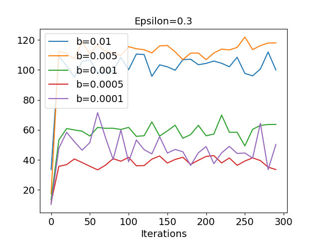
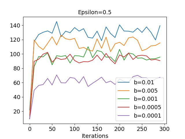
In figure 6 we show the trend that smaller $b$ works better for larger $\epsilon$ and larger $b$ works better for smaller $\epsilon$ in general. This can be explained in the following way: with a larger $\epsilon$ the data distribution is more exploratory and hence the probabilities on individual state, action pairs are smaller. So a the same threshold that performs well with low exploration now censors a much larger part of the state, action space, necessitating a smaller threshold as $\epsilon$ is increased. In general, we find that having the largest threshold which still retains a significant fraction of the state, action space is a good heuristic for setting the $b$ parameter.

Appendix F Details of Hopper-v3 Experiment

In this section we introduce some missing details about the MBS-QL algorithm and the experimental details. We also attach the complete code for running our algorithm and the baseline algorithms in the supplemental materials.

F.1 Implementation Details of MBS-QL

MBS-QL algorithm is implemented based on the architecture of Batch-Constrained deep $Q$-learning (BCQ) [11] algorithm. More specifically, we use the similar Clipped Double Q-Learning (CDQ) update rule for the $Q$ learning part, and employ a similar variational auto-encoder to fit the conditional action distribution in the batch. We use an additional variational auto-encoder to fit the marginalized state distribution of the batch. To implement an actual $Q$ learning algorithm instead of an actor-critic algorithm, we did not sample from the actor in the Bellman backup but sample a larger batch from the fitted conditional action distribution. Algorithm 4 shows the pseudo-code of MBS-QL to provide more details. We highlight the difference with the BCQ algorithm in red.

Algorithm 4 MBS $Q$-learning (MBS-QL)
Input: Batch $D$, ELBO threshold $b$, maximum perturbation $\Phi$, target update rate $\tau$, mini-batch size $N$, max number of iteration $T$. Number of actions $k$.
Initialize two Q network $Q_{\theta_{1}}$ and $Q_{\theta_{2}}$, policy (perturbation) model: $\xi_{\phi}$. ($\xi_{\phi}\in[-\Phi,\Phi]$), action VAE $G^{a}_{\omega_{1}}$ and state VAE Gฯ‰2ssubscriptsuperscript๐บ๐‘ subscript๐œ”2G^{s}_{\omega_{2}}.
Pretrain Gฯ‰2ssubscriptsuperscript๐บ๐‘ subscript๐œ”2G^{s}_{\omega_{2}}: ฯ‰2โ†argโ€‹minฯ‰2โกEโ€‹Lโ€‹Bโ€‹Oโ€‹(B;Gฯ‰2s)โ†subscript๐œ”2subscriptargminsubscript๐œ”2๐ธ๐ฟ๐ต๐‘‚๐ตsubscriptsuperscript๐บ๐‘ subscript๐œ”2\omega_{2}\leftarrow\operatorname*{arg\,min}_{\omega_{2}}ELBO(B;G^{s}_{\omega_{2}}).
forย t=1๐‘ก1t=1 to $T$ย do
ย ย ย ย ย Sample a minibatch $B$ with $N$ samples from $D$.
ย ย ย ย ย ฯ‰1โ†argโ€‹minฯ‰2โกEโ€‹Lโ€‹Bโ€‹Oโ€‹(B;Gฯ‰1a)โ†subscript๐œ”1subscriptargminsubscript๐œ”2๐ธ๐ฟ๐ต๐‘‚๐ตsubscriptsuperscript๐บ๐‘Žsubscript๐œ”1\omega_{1}\leftarrow\operatorname*{arg\,min}_{\omega_{2}}ELBO(B;G^{a}_{\omega_{1}}).
ย ย ย ย ย Sample $k$ actions $a^{\prime}_{i}$ from Gฯ‰1aโ€‹(sโ€ฒ)subscriptsuperscript๐บ๐‘Žsubscript๐œ”1superscript๐‘ โ€ฒG^{a}_{\omega_{1}}(s^{\prime}) for each sโ€ฒsuperscript๐‘ โ€ฒs^{\prime}.
ย ย ย ย ย Compute the target $y$ for each (s,a,r,sโ€ฒ)๐‘ ๐‘Ž๐‘Ÿsuperscript๐‘ โ€ฒ(s,a,r,s^{\prime}) pair:
y=r+ฮณโ€‹๐Ÿ™โ€‹(Eโ€‹Lโ€‹Bโ€‹Oโ€‹(sโ€ฒ;Gฯ‰2s)โ‰ฅb)โ€‹[maxaiโ€ฒโก(0.75โˆ—minj=1,2โกQฮธjโ€ฒ+0.25โˆ—maxj=1,2โกQฮธjโ€ฒ)]๐‘ฆ๐‘Ÿ๐›พ1๐ธ๐ฟ๐ต๐‘‚superscript๐‘ โ€ฒsubscriptsuperscript๐บ๐‘ subscript๐œ”2๐‘delimited-[]subscriptsubscriptsuperscript๐‘Žโ€ฒ๐‘–0.75subscript๐‘—12subscript๐‘„subscriptsuperscript๐œƒโ€ฒ๐‘—0.25subscript๐‘—12subscript๐‘„subscriptsuperscript๐œƒโ€ฒ๐‘—y=r+\gamma{\color[rgb]{1,0,0}\mathds{1}(ELBO(s^{\prime};G^{s}_{\omega_{2}})\geq b)}\left[\max_{a^{\prime}_{i}}\left(0.75*\min_{j=1,2}Q_{\theta^{\prime}_{j}}+0.25*\max_{j=1,2}Q_{\theta^{\prime}_{j}}\right)\right]
ย ย ย ย ย ฮธโ†argโ€‹minฮธโ€‹โˆ‘(yโˆ’Qฮธโ€‹(s,a))2โ†๐œƒsubscriptargmin๐œƒsuperscript๐‘ฆsubscript๐‘„๐œƒ๐‘ ๐‘Ž2\theta\leftarrow\operatorname*{arg\,min}_{\theta}\sum(y-Q_{\theta}(s,a))^{2}
ย ย ย ย ย Sample $k$ actions $a_{i}$ from Gฯ‰1aโ€‹(s)subscriptsuperscript๐บ๐‘Žsubscript๐œ”1๐‘ G^{a}_{\omega_{1}}(s) for each s๐‘ s.
ย ย ย ย ย ฯ•โ†argโ€‹maxฯ•โ€‹โˆ‘maxaiโกQฮธ1โ€‹(s,ai+ฮพฯ•โ€‹(s,ai))โ†italic-ฯ•subscriptargmaxitalic-ฯ•subscriptsubscript๐‘Ž๐‘–subscript๐‘„subscript๐œƒ1๐‘ subscript๐‘Ž๐‘–subscript๐œ‰italic-ฯ•๐‘ subscript๐‘Ž๐‘–\phi\leftarrow\operatorname*{arg\,max}_{\phi}\sum\max_{a_{i}}Q_{\theta_{1}}(s,a_{i}+\xi_{\phi}(s,a_{i}))
ย ย ย ย ย Update target network: $\theta^{\prime}=(1-\tau)\theta^{\prime}+\tau\theta$, $\phi^{\prime}=(1-\tau)\phi^{\prime}+\tau\phi$
endย for
When evaluate the resulting policy: select action a=argโ€‹maxaiโกQฮธ1โ€‹(s,ai+ฮพฯ•โ€‹(s,ai))๐‘Žsubscriptargmaxsubscript๐‘Ž๐‘–subscript๐‘„subscript๐œƒ1๐‘ subscript๐‘Ž๐‘–subscript๐œ‰italic-ฯ•๐‘ subscript๐‘Ž๐‘–a=\operatorname*{arg\,max}_{a_{i}}Q_{\theta_{1}}(s,a_{i}+\xi_{\phi}(s,a_{i})) where $a_{i}$ are $k$ actions sampled from Gฯ‰1aโ€‹(s)subscriptsuperscript๐บ๐‘Žsubscript๐œ”1๐‘ G^{a}_{\omega_{1}}(s) given s๐‘ s.

In practice, the indicator function ๐Ÿ™โ€‹(Eโ€‹Lโ€‹Bโ€‹Oโ€‹(sโ€ฒ;Gฯ‰2s)โ‰ฅb)1๐ธ๐ฟ๐ต๐‘‚superscript๐‘ โ€ฒsubscriptsuperscript๐บ๐‘ subscript๐œ”2๐‘\mathds{1}(ELBO(s^{\prime};G^{s}_{\omega_{2}})\geq b) is implemented by sigmoidโ€‹(100โ€‹(Eโ€‹Lโ€‹Bโ€‹Oโ€‹(sโ€ฒ;Gฯ‰2s)โˆ’b))sigmoid100๐ธ๐ฟ๐ต๐‘‚superscript๐‘ โ€ฒsubscriptsuperscript๐บ๐‘ subscript๐œ”2๐‘\text{sigmoid}(100(ELBO(s^{\prime};G^{s}_{\omega_{2}})-b)) to provide a slightly more smooth target. The evidence lower bound (ELBO) objective function of VAE is:

$\displaystyle ELBO(s;G^{s}_{\omega_{2}})=\sum(s-\tilde{s})^{2}+D_{\text{KL}}(N(\mu,\sigma)||N(0,1))$ (123)

where $\mu$ and $\sigma$ is sampled from the encoder of VAE with input s๐‘ s and s~~๐‘ \tilde{s} is sampled from the decoder with the hidden state generated from $N(\mu,\sigma)$. Eโ€‹Lโ€‹Bโ€‹Oโ€‹(B;Gฯ‰2s)๐ธ๐ฟ๐ต๐‘‚๐ตsubscriptsuperscript๐บ๐‘ subscript๐œ”2ELBO(B;G^{s}_{\omega_{2}}) is the averaged ELBO on the minibatch $B$. So does $G^{a}_{\omega_{1}}$. Note that this ELBO objective make the implicit assumption that the decoderโ€™s distribution is a Gaussian distribution with mean equals to the output of decoder network. So when we generate the sample $a^{\prime}$ for computing $y$, we add a Gaussian noise $N(0,1.5)$ to the output of decoder network.

F.2 Experimental details

We collect the batch data using a near-optimal policy with two-level noise, which is the same setting as the โ€œImperfect Imitationโ€ in the BCQ paper [11]. We first get the near-optimal policy by running DDPG in 15 random seeds and pick the best 5 resulting policies. Then with probability $0.3$ it samples uniformly from action space, with probability $0.7$ it adds a Gaussian noise $\mathcal{N}(0,0.3)$ to the action from DDPG policy.

For most of the hyper-parameters in Algorithm 4, we use the same value with the BCQ algorithm. We run all algorithms with $T=10^{6}$ gradient steps, and the minibatch size $N=100$ at each step. The number of action $k=100$. Target network update rate is $0.005$. The threshold $b$ of ELBO is selected as $2$-percentile of the Eโ€‹Lโ€‹Bโ€‹Oโ€‹(s)๐ธ๐ฟ๐ต๐‘‚๐‘ ELBO(s) in the whole dataset after pretrain the VAE.

A key hyper-parameter in BCQ is the maximum perturbation $\Phi$. It controls the amount of difference with the behavior cloning allowed by the BCQ algorithm. The results in Appendix D.1 of their paper [11] suggest a smaller $\Phi$ is always better and they use $\Phi=0.05$ to report their results. For our algorithm, we find that the performance is not monotonic with $\Phi$, which might suggest some more interesting behavior of our algorithm since it is less similar to behavior cloning. In Figure 7 we report an ablation study of perturbation bound $\Phi$. We compare MBS-QL and BCQ with $\Phi=0.05,0.1$ and $0.25$. For all values of $\Phi$ MBS-QL is better than BCQ with the same $\Phi$. For the results in main paper, we use $\Phi=0.1$ for MBS-QL and $\Phi=0.05$ for BCQ.

Refer to caption
Figure 7: BCQ [11] and MBS-QL with different range of policy output ($\Phi$).