Combining Task Predictors
via Enhancing Joint Predictability

Abstract

Predictor combination aims to improve a (target) predictor of a learning task based on the (reference) predictors of potentially relevant tasks, without having access to the internals of individual predictors. We present a new predictor combination algorithm that improves the target by i) measuring the relevance of references based on their capabilities in predicting the target, and ii) strengthening such estimated relevance. Unlike existing predictor combination approaches that only exploit pairwise relationships between the target and each reference, and thereby ignore potentially useful dependence among references, our algorithm jointly assesses the relevance of all references by adopting a Bayesian framework. This also offers a rigorous way to automatically select only relevant references. Based on experiments on seven real-world datasets from visual attribute ranking and multi-class classification scenarios, we demonstrate that our algorithm offers a significant performance gain and broadens the application range of existing predictor combination approaches.

1 Introduction

Many practical visual understanding problems involve learning multiple tasks. When a target predictor, e.g. a classification or a ranking function tailored for the task at hand, is not accurate enough, one could benefit from knowledge accumulated in the predictors of other tasks (references). The predictor combination problem studied by Kim et al. [KimTomRic17] aims to improve the target predictor by exploiting the references without requiring access to the internals of any predictors or assuming that all predictors belong to the same class of functions. This is relevant when the forms of predictors are not known (e.g. precompiled binaries) or the best predictor forms differ across tasks. For example, Gaussian process rankers [Joachims2002] trained on ResNet101 features [HeZhaRen16] are identified as the best for the main task, e.g. for image frame retrieval, while convolutional neural networks are presented as a reference, e.g. classification of objects in images. In this case, existing transfer learning or multi-task learning approaches, such as a parameter or weight sharing, cannot be applied directly.

Kim et al. [KimTomRic17] approached this predictor combination problem for the first time by nonparametrically accessing all predictors based on their evaluations on given datasets, regarding each predictor as a Gaussian process (GP) estimator. Assuming that the target predictor is a noisy observation of an underlying ground-truth predictor, their algorithm projects all predictors onto a Riemannian manifold of GPs and denoises the target by simulating a diffusion process therein. This approach has demonstrated a noticeable performance gain while meeting the challenging requirements of the predictor combination problem. However, it leaves three possibilities to improve. Firstly, this algorithm is inherently (pairwise) metric-based and, therefore, it can model and exploit only pairwise relevance of the target and each reference, while relevant information can lie in the relationship between multiple references. Secondly, this algorithm assumes that all references are noise-free, while in practical applications, the references may also be trained based on limited data points or weak features and thus they can be imperfect. Thirdly, as this algorithm uses the metric defined between GPs, it can only combine one-dimensional target and references.

In this paper, we propose a new predictor combination algorithm that overcomes these three challenges. The proposed algorithm builds on the manifold denoising framework [KimTomRic17] but instead of their metric diffusion process, we newly pose the predictor denoising as an averaging process, which jointly exploits full dependence of the references. Our algorithm casts the denoising problem into 1) measuring the joint capabilities of the references in predicting the target, and 2) optimizing the target as a variable to enhance such prediction capabilities. By adopting Bayesian inference under this setting, identifying relevant references is now addressed by a rigorous Bayesian relevance determination approach. Further, by denoising all predictors in a single unified framework, our algorithm becomes applicable even for imperfect references. Lastly, our algorithm can combine multi-dimensional target and reference predictors, e.g. it can improve multi-class classifiers based on one-dimensional rank predictors. Experiments on relative attribute ranking and multi-class classification demonstrate that these contributions individually and collectively improve the performance of predictor combination and further extend the application domain of existing predictor combination algorithms.

Related work. Transfer learning (TL) aims to solve a given learning problem by adapting a source model trained on a different problem [PanYan10]. Predictor combination can be regarded as a specific instance of TL. However, unlike predictor combination algorithms, traditional TL approaches improve or newly train predictors of known form. Also, most existing algorithms assume that the given source is relevant to the target and, therefore, they do not explicitly consider identifying relevant predictors among many (potentially irrelevant) source predictors.

Another related problem is multi-task learning (MTL), which learns predictors on multiple problems at once [ArgEvgPon08, CheZhaLi14]. State-of-the-art MTL algorithms offer the capability of automatically identifying relevant task groups when not all tasks and the corresponding predictors are mutually relevant. For example, Argyriou et al. [ArgEvgPon08] and Gong et al. [GonYeZhang12], respectively, enforced the sparsity and low-rank constraints in the parameters of predictors to make them aggregate in relevant task groups. Passos et al. [PasRaiWai12] performed explicit task clustering ensuring that all tasks (within a cluster) that are fed to the MTL algorithm are relevant. More recently, Zamir et al. [ZamSaxShe18] proposed to discover a hypergraph that reveals the interdependence of multiple tasks and facilitates transfer of knowledge across relevant tasks.

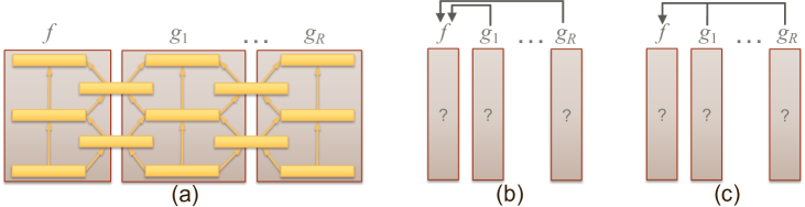
Figure 1: Illustration of predictor combination algorithms: (a) MTL simultaneously exploits all references $\{g_{1},\ldots,g_{R}\}$ to improve the target predictor $f$, e.g. by sharing neural network layers. However, they require access to the internals of predictors [CheZhaLi14]. (b) Kim et al.’s predictor combination is agnostic to the forms of individual predictors [KimTomRic17] but exploits only pairwise relationships. (c) Our algorithm combines the benefits of both, jointly exploiting all references without requiring their known forms.

While our approach has been motivated by the success of TL and MTL approaches, these approaches are not directly applicable to predictor combination as they share knowledge across tasks via the internal parametric representations [ArgEvgPon08, GonYeZhang12, PasRaiWai12] and/or shared deep neural network layers of all predictors (e.g. via shared encoder readouts [ZamSaxShe18]; see Fig. 1). A closely related approach in this context is Mejjati et al.’s nonparametric MTL approach [MejCosKim18]. Similar to Kim et al. [KimTomRic17], this algorithm assesses predictors based on their sample evaluations, and it (nonparametrically) measures and enforces pairwise statistical dependence among predictors. As this approach is agnostic to the forms of individual predictors, it can be adapted for predictor combination. However, this algorithm shares the same limitations: it can only model pairwise relationships. We demonstrate experimentally that by modeling the joint relevance of all references, our algorithm can significantly outperform both Kim et al.’s original predictor combination algorithm [KimTomRic17] adapted to ranking [KimCha19], and Mejjati et al.’s MTL algorithm [MejCosKim18].

2 The predictor combination problem

Suppose we have an initial predictor $f^{0}\colon\mathcal{X}\to\mathcal{Y}$ (e.g. a classification, regression, or ranking function) of a task. The goal of predictor combination is to improve the target predictor $f^{0}$ based on a set of reference predictors $\mathcal{G}=\{g_{i}\colon\mathcal{X}\to\mathcal{Y}_{i}\}_{i=1}^{R}$. The internal structures of the target and reference predictors are unknown and they might have different forms. Crucial to the success of addressing this seriously ill-posed problem is to determine which references (if any) within $\mathcal{G}$ are relevant (i.e. useful in improving $f^{0}$), and to design a procedure that fully exploits such relevant references without requiring access to the internals of $f^{0}$ and $\mathcal{G}$.

Kim et al.’s original predictor combination (OPC) [KimTomRic17] approaches this problem by 1) considering the initial predictor $f^{0}$ as a noisy estimate of the underlying ground-truth $f_{\text{GT}}$, and 2) assuming $f_{\text{GT}}$ and $\mathcal{G}$ are structured such that they all lie on a low-dimensional predictor manifold $\mathcal{M}$. These assumptions enable predictor combination to be cast as well-established Manifold Denoising, where one iteratively denoises points on $\mathcal{M}$ via simulating the diffusion process therein [HeiMai07].

The model space $\mathcal{M}$ of OPC consists of Bayesian estimates: each predictor in $\mathcal{M}$ is a GP predictive distribution of the respective task. The natural metric $g_{\mathcal{M}}$ on $\mathcal{M}$, in this case, is induced from the Kullback-Leibler (KL) divergence $D_{\text{KL}}$ between probability distributions. Now further assuming that all reference predictors are noise-free, their diffusion process is formulated as a time-discretized evolution of $f^{t}$ on $\mathcal{M}$: Given the solution $f^{t}$ at time $t$ and noise-free references $\mathcal{G}$, the new solution $f^{t+1}$ is obtained by minimizing the energy

$$\mathcal{E}_{\text{O}}(f) =D_{\text{KL}}^{2}(f\mid f^{t})+\lambda_{\text{O}}\sum_{i=1}^{R}w_{i}D_{\text{KL}}^{2}(f\mid g_{i})\text{,}$$ (1)

where $w_{i}\!=\!\exp(-D_{\text{KL}}^{2}(f^{t}\mid g_{i})/\sigma^{2}_{\text{O}})$ is inversely proportional to $D_{\text{KL}}(f^{t}\mid g_{i})$, and $\lambda_{\text{O}}$ and $\sigma^{2}_{\text{O}}$ are hyperparameters. Our supplemental document presents how the iterative minimization of $\mathcal{E}_{\text{O}}$ is obtained by discretizing the diffusion process on $\mathcal{M}$.

In practice, it is infeasible to directly optimize functions, which are infinite-dimensional objects. Instead, OPC approximates all predictors $\{f,\mathcal{G}\}$ via their evaluations on a test dataset $X\!=\!\{\mathbf{x}_{1},\ldots,\mathbf{x}_{N}\}$, and optimizes the sample $f$-evaluation $\mathbf{f}=f|_{X}:=[f(\mathbf{x}_{1}),\ldots,f(\mathbf{x}_{N})]^{\top}$ based on the sample references $\mathcal{G}=\{\mathbf{g}_{1},\ldots,\mathbf{g}_{R}\}$ with $\mathbf{g}_{i}=g_{i}|_{X}$.

At each time step, the relevance of a reference is automatically determined based on its KL-divergence to the current solution: $g_{i}$ is considered relevant when $D_{\text{KL}}(f^{t}\mid g_{i})$ is small. Then, throughout the iteration, OPC robustly denoises $f$ by gradually putting more emphasis on highly relevant references while ignoring outliers. This constitutes the first predictor combination algorithm that improves the target predictor without requiring any known forms of predictors (as the KL-divergences are calculated purely based on predictor evaluations). However, Eq. 31 also highlights the limitations of this approach: it exploits only pairwise relationships between the target predictor and individual references, ignoring the potentially useful information that lies in the dependence between references.

Toy problem 1. Consider two references, $\{\mathbf{g}_{1},\!\mathbf{g}_{2}\}\!\subset\!\mathbb{R}^{100}$, constructed by uniformly randomly sampling from $\{0,1\}$. Here, $\{\mathbf{g}_{1},\mathbf{g}_{2}\}$ are regarded as the means of GP predictive distributions with unit variances. We define the ground-truth target as their difference: $\mathbf{f}_{\text{GT}}=\mathbf{g}_{1}-\mathbf{g}_{2}$. By construction, $\mathbf{f}_{\text{GT}}$ is determined by the relationship between the references. Now we construct the initial noisy predictor $\mathbf{f}^{0}$ by adding independent Gaussian noise with standard deviation $1$ to $\mathbf{f}_{\text{GT}}$, achieving the rank accuracy of $0.67$ (see Sec. 4 for the definition of the visual attribute ranking problem). In this case, applying OPC minimizes $\mathcal{E}_{\text{O}}$ (Eq. 31) but shows insignificant performance improvement as no information on $\mathbf{f}_{\text{GT}}$ can be gained by assessing the relevance of the references individually (Table 1). While this problem has been well-studied in existing MTL and TL approaches, the application of these techniques for predictor combination is not straightforward as they require simultaneous training [GonYeZhang12, PasRaiWai12] and/or shared predictor forms [ZamSaxShe18]. Another limitation is that OPC requires that all predictions are one-dimensional (i.e. $\mathcal{Y}_{i}\subset\mathbb{R}$). Therefore, it is not capable of, for example, improving the multi-class classification predictor $\mathbf{f}^{0}$ given the references constructed for ranking tasks.

Table 1: Accuracies of Kim et al.’s original (OPC) [KimTomRic17], and our linear (LPC) and nonlinear (NPC) predictor combination algorithms introduced in Section 3, for illustrative toy problems. $\mathbf{g}_{1}$ and $\mathbf{g}_{2}$ are random binary vectors while $\mathbf{f}^{0}$’s are noisy observations of the corresponding ground-truth predictors $\mathbf{f}_{\text{GT}}$’s.

Toy problem	$\mathbf{f}^{0}$	OPC [KimTomRic17] (Eq. 31)	LPC (Eq. 7)	NPC (Eq. 27)
1: $\mathbf{f}_{\text{GT}}=\mathbf{g}_{1}-\mathbf{g}_{2}$	67.14	67.24	100	100
2: $\mathbf{f}_{\text{GT}}=\text{XOR}(\mathbf{g}_{1},\mathbf{g}_{2})$	74.08	74.11	74.24	100

3 Joint predictor combination algorithm

Our algorithm takes deterministic predictors instead of Bayesian predictors (i.e. GP predictive distributions) as in OPC. When Bayesian predictors are provided as inputs, we simply take their means and discard the predictive variances. This design choice offers a wider range of applications as most predictors – including deep neural networks and support vector machines (SVMs) – are presented as deterministic functions, at the expense of not exploiting potentially useful predictive uncertainties. This assumption has also been adopted by Kim and Chang [KimCha19]. Under this setting, our model space is a sub-manifold $\mathcal{M}$ of $L^{2}$ space where each predictor has zero mean and unit norm:

$$\forall f\in\mathcal{M}.\quad\int f(\mathbf{x})\mathrm{d}P(\mathbf{x})=0\quad\text{and}\quad\langle f,f\rangle=1\text{,}$$ (2)

where $\langle f,g\rangle:=\int f(\mathbf{x})g(\mathbf{x})dP(\mathbf{x})$ and $P(\mathbf{x})$ is the probability distribution of $\mathbf{x}$. This normalization enables scale and shift-invariant assessment of the relevance of references. The Riemannian metric $g_{\mathcal{M}}$ on $\mathcal{M}$ is defined as the pullback metric of the ambient $L^{2}$ space: when $\mathcal{M}$ is embedded into $L^{2}$ via the embedding $\imath$, $g_{\mathcal{M}}(a,b):=\langle\imath(a),\imath(b)\rangle$. OPC (Eq. 31) can be adapted for $\mathcal{M}$ by iteratively maximizing the objective $\mathcal{O}_{\text{O}}$ that replaces the KL-divergence $D_{\text{KL}}$ with $g_{\mathcal{M}}(\cdot,\cdot)$:

$$\mathcal{O}_{\text{O}}(f) =g_{\mathcal{M}}(f,f^{t})^{2}+\lambda_{\text{O}}\sum_{i=1}^{R}w_{i}g_{\mathcal{M}}(f,g_{i})^{2}\text{.}$$ (3)

For simplicity of exposition, we here assume that the output space is one-dimensional (i.e. $\mathcal{Y}_{i}=\mathbb{R}$). In Sec. 4, we show how this framework can be extended to multi-dimensional outputs such as for multi-class classification.

The averaging process on $\cal\mathcal{M}$. Both OPC (Eq. 31) and its adaptation to our model space (Eq. 3) can model only the pairwise relationship between the target $f$ and each reference $g_{i}\in\mathcal{G}$, while ignoring the dependence present across the references (joint relevance of $\mathcal{G}$ on $f$). We now present a general framework that can capture such joint relevance by iteratively maximizing the objective

$$\mathcal{O}_{\text{J}}(f) =\langle\imath(f),\imath(f^{t})\rangle^{2}+\lambda_{\text{J}}\langle\imath(f),\mathcal{K}[\imath(f)]\rangle\text{,}$$ (4)

where $\lambda_{\text{J}}\geq 0$ is a hyperparameter. The linear, non-negative definite averaging operator $\mathcal{K}\colon\imath(\mathcal{M})\to\imath(\mathcal{M})$ is responsible to capture the joint relevance of $\mathcal{G}$ on $f$. Depending on the choice of $\mathcal{K}$, $\mathcal{O}_{\text{J}}$ can accommodate a variety of predictor combination scenarios, including $\mathcal{O}_{\text{O}}$ as a special case for $\mathcal{K}[\imath(f)]=\sum_{i=1}^{R}\imath(g_{i})w_{i}\langle\imath(f),\imath(g_{i})\rangle$.

3.1 Linear predictor combination (LPC)

Our linear predictability operator $\mathcal{K}_{\text{L}}$ is defined as

$$\mathcal{K}_{\text{L}}[\imath(f)]=\sum_{i,j=1}^{R}\imath(g_{i})C^{-1}_{[i,j]}\langle\imath(g_{j}),\imath(f)\rangle$$ (5)

using the correlation matrix $C_{[i,j]}=\langle\imath(g_{i}),\imath(g_{j})\rangle$. Interpreting $\mathcal{K}_{\text{L}}$ becomes straightforward when substituting $\mathcal{K}_{\text{L}}$ into the second term of $\mathcal{O}_{\text{J}}$ (Eq. 4):

$$\langle\imath(f),\mathcal{K}_{\text{L}}[\imath(f)]\rangle=\mathbf{c}^{\top}C^{-1}\mathbf{c}\text{,}$$ (6)

where $\mathbf{c}=[\langle\imath(f),\imath(g_{1})\rangle,\ldots,\langle\imath(f),\imath(g_{R})\rangle]^{\top}$. As each predictor in $\mathcal{M}$ is centered and normalized, all diagonal elements of the correlation matrix $C$ are $1$. The off-diagonal elements of $C$ then represent the dependence among the references, making $\langle\imath(f),\mathcal{K}_{\text{L}}[\imath(f)]\rangle$ a measure of joint correlation between $f$ and $\mathcal{G}=\{g_{i}\}_{i=1}^{R}$.

In practice, $f$ and $\{g_{i}\}$ might not be originally presented as embedded elements $\imath(f)$ and $\{\imath(g_{i})\}$ of $\mathcal{M}$: i.e. they are not necessarily centered or normalized (Eq. 2). Also, as in the case of OPC, it would be infeasible to manipulate infinite-dimensional functions directly. Therefore, we also adopt sample approximations $\{\mathbf{f},\mathbf{g}_{1},\ldots,\mathbf{g}_{R}\}$ and explicitly project them onto $\mathcal{M}$ via normalization: $\mathbf{f}\to\overline{\mathbf{f}}:=\frac{C_{N}\mathbf{f}}{\|C_{N}\mathbf{f}\|}$, where $C_{N}\!=\!\mathbf{1}_{N\times N}/N$, $\mathbf{1}_{N\times N}$ is an $N\!\times\!N$ matrix of ones, for the sample size $N\!=\!|X|$. For this scenario, we obtain our linear predictor combination (LPC) algorithm by substituting Eq. 5 into Eq. 4, and replacing $f$, $f^{t}$, and $g_{j}$ by $\overline{\mathbf{f}}$, $\overline{\mathbf{f}}^{t}$, and $\overline{\mathbf{g}}_{j}$, respectively:

$$\mathcal{O}_{\text{L}}(\mathbf{f}) =\frac{(\mathbf{f}^{\top}\overline{\mathbf{f}^{t}})^{2}}{\mathbf{f}^{\top}C_{N}\mathbf{f}}+\lambda_{\text{J}}\mathcal{P}_{\text{L}}\text{,}$$ (7)

where $\mathcal{P}_{\text{L}}=\frac{\mathbf{f}^{\top}Q\mathbf{f}}{\mathbf{f}^{\top}C_{N}\mathbf{f}}$, $Q=G(G^{\top}G)^{-1}G$, and $G=[\overline{\mathbf{g}}_{1},\ldots,\overline{\mathbf{g}}_{R}]$. Here, we pre-projected $\mathcal{G}$ and $\mathbf{f}^{t}$ onto $\mathcal{M}$ while $\mathbf{f}$ is explicitly projected in Eq. 7. Note that our goal is not to simply calculate $\mathcal{P}_{\text{L}}$ for a fixed $\mathbf{f}$, but to optimize $\mathbf{f}$ while enhancing $\mathcal{P}_{\text{L}}$.

Exploiting the joint relevance of references, LPC can provide significant accuracy improvements over OPC. For example, LPC can generate perfect predictions in Toy Problem 1 (Table 1). However, its capability in measuring the joint relevance is limited to linear relationships only. This can be seen by rewriting $\mathcal{P}_{\text{L}}$ explicitly in $\mathbf{f}$ and $G$:

$$\mathcal{P}_{\text{L}}=\frac{\mathbf{f}^{\top}Q\mathbf{f}}{\mathbf{f}^{\top}C_{N}\mathbf{f}}=1-\frac{\sum_{i=1}^{N}(\mathbf{f}_{i}-q(G_{[i,:]}))^{2}}{\sum_{i=1}^{N}(\mathbf{f}_{i}-\sum_{j=1}^{n}\mathbf{f}_{j}/N)^{2}}\text{,}$$ (8)

where $G_{[i,:]}$ represents the $i$-th row of $G$, and $q(\mathbf{a})=\mathbf{w}_{q}^{\top}\mathbf{a}$ is the linear function whose weight vector $\mathbf{w}_{q}=(G^{\top}G)^{-1}G\mathbf{f}$ is obtained from least-squares regression that takes the reference matrix $G$ as training input and the target predictor variable $\mathbf{f}$ as corresponding labels. Then, $\mathcal{P}_{\text{L}}$ represents the normalized prediction accuracy: the normalizer $\mathbf{f}^{\top}C_{N}\mathbf{f}$ is simply the variance of $\mathbf{f}$ elements. For this reason, we call $\mathcal{P}_{\text{L}}$ the (linear) predictability of $G$ (and equivalently of $\mathcal{G}$) on $\mathbf{f}$. It takes the maximum value of 1 when the linear prediction (made based on $G$) perfectly agrees with $\mathbf{f}$ when normalized, and it attains the minimum value 0 when the prediction is no better than taking the mean value of $\mathbf{f}$, in which case the mean squared error becomes the variance. Figure 1 illustrates our algorithm in comparison with MTL and OPC.

Toy problem 2. Under the setting of Toy problem 1, when the target $\mathbf{f}_{\text{GT}}$ is replaced by a variable that is nonlinearly related to the references, e.g. using the logical exclusive OR (XOR) of $\mathbf{g}_{1}$ and $\mathbf{g}_{2}$, LPC fails to give any noticeable accuracy improvement compared to the baseline $\mathbf{f}^{0}$.

3.2 Nonlinear predictor combination (NPC)

Our final algorithm measures the relevance of $\mathcal{G}$ on $\mathbf{f}$ by predicting $\mathbf{f}$ via Gaussian process (GP) estimation. We use the standard zero-mean Gaussian prior and an i.i.d. Gaussian likelihood with noise variance $\sigma^{2}$ [RasWill06]. The resulting prediction is obtained as a Gaussian distribution with mean $\mathbf{m}_{\mathbf{f}}$ and covariance $C_{\mathbf{f}}$:

$$\kern-3.00003pt\mathbf{m}_{\mathbf{f}}\!=\!K(K\!+\!\sigma^{2}I)^{-1}\mathbf{f}\text{,}\enskip\;C_{\mathbf{f}}\!=\!K\!-\!K(K\!+\!\sigma^{2}I)^{-1}K\text{,}\kern-3.00003pt$$ (9)

where $K\in\mathbb{R}^{N\times N}$ is defined using the covariance function $k\colon\mathbb{R}^{R}\times\mathbb{R}^{R}\to\mathbb{R}$:

$$K_{[i,j]}=k(G_{[i,:]},G_{[j,:]}):=\exp\left(-\frac{\|G_{[i,:]}-G_{[j,:]}\|^{2}}{\sigma_{k}^{2}}\right)\text{.}$$ (10)

Now we refine the linear predictability $\mathcal{P}_{\text{L}}$ by replacing $q(G_{[i,:]})$ in Eq. 8 with the corresponding predictive mean $[\mathbf{m}_{\mathbf{f}}]_{i}$ (where $[\mathbf{a}]_{i}$ is the $i$-th element of vector $\mathbf{a}$):

$$\mathcal{P}_{\text{N}}=\frac{\mathbf{f}^{\top}Q^{\prime}\mathbf{f}}{\mathbf{f}^{\top}C_{N}\mathbf{f}}=1-\frac{\sum_{i=1}^{N}([\mathbf{f}]_{i}-[\mathbf{m}_{\mathbf{f}}]_{i})^{2}}{\sum_{i=1}^{N}([\mathbf{f}]_{i}-\sum_{j=1}^{N}[\mathbf{f}]_{j}/N)^{2}}\text{,}$$ (11)

where $Q^{\prime}$ is a positive definite matrix that replaces $Q$ in Eq. 8:

$$Q^{\prime}=C_{N}\left(2K(K+\sigma^{2}I)^{-1}-(K+\sigma^{2}I)^{-1}KK(K+\sigma^{2}I)^{-1}\right)C_{N}\text{.}$$ (12)

The matrix $Q^{\prime}$ becomes $Q$ when the kernel $k(\mathbf{a},\mathbf{b})$ is replaced by the standard dot product $k^{\prime}(\mathbf{a},\mathbf{b})=\mathbf{a}^{\top}\mathbf{b}$. Note that the noise level $\sigma^{2}$ should be strictly positive; otherwise, $\mathbf{f}_{i}=[\mathbf{m}_{\mathbf{f}}]_{i}$ for all $i\in\{1,\ldots,N\}$, and therefore $\mathcal{P}_{\text{N}}=1$ for any $\mathbf{f}$. This means the resulting GP model perfectly overfits to $\mathbf{f}$ and all references are considered perfectly relevant regardless of the actual values of $G$ and $\mathbf{f}$.

Computational model. Explicitly normalizing $\mathbf{f}$ ($\mathbf{f}\to\overline{\mathbf{f}}$) in the nonlinear predictability $\mathcal{P}_{\text{N}}$ (Eq. 11), substituting $Q^{\prime}$ into $\mathcal{P}_{\text{N}}$, and then replacing $\mathcal{P}_{\text{L}}$ with $\mathcal{P}_{\text{N}}$ in $\mathcal{O}_{\text{L}}$ (Eq. 7) yields the following Rayleigh quotient-type objective to maximize:

$$\mathcal{O}_{\text{N}}(\mathbf{f})=\frac{\mathbf{f}^{\top}A\mathbf{f}}{\mathbf{f}^{\top}C_{N}\mathbf{f}}\text{,}\quad A=(C_{N}\mathbf{f}^{t})(C_{N}\mathbf{f}^{t})^{\top}+\lambda_{\text{J}}Q^{\prime}\text{.}$$ (13)

For any non-negative definite matrices $A$ and $C_{N}$, the maximizer of the Rayleigh quotient $\mathcal{O}_{\text{N}}$ is the largest eigenvector (the eigenvector corresponding to the maximum eigenvalue) of the generalized eigenvector problem $A\mathbf{f}=\lambda C_{N}\mathbf{f}$. The computational complexity of solving the generalized eigenvector problem of matrices $\{A,C_{N}\}\subset\mathbb{R}^{N\times N}$ is $O(N^{3})$. As in our case $N=|X|$, solving this problem is infeasible for large-scale problems. To obtain a computationally affordable solution, we first note that $A$ incorporates multiplications by the centering matrix $C_{N}$ and, therefore, all eigenvectors of $A$ are centered, which implies that they are also eigenvectors of $C_{N}$. This effectively renders the generalized eigenvector problem into the standard eigenvector problem of matrix $A$.

Secondly, we make sparse approximate GP inference by adopting a low-rank approximation of $K$ [SeeIllLaw03]:

$$K\approx K_{GB}K_{BB}^{-1}K_{GB}^{\top}\text{, }{K_{GB}}_{[i,j]}=k(G_{[i,:]},B_{[j,:]})\text{, }{K_{BB}}_{[i,j]}=k(B_{[i,:]},B_{[j,:]})\text{,}$$ (14)

where the $i$-th row $B_{[i,:]}$ of $B\in\mathbb{R}^{N^{\prime}\times R}$ represents the $i$-th basis vector. We construct the basis vector matrix $B$ by linearly sampling $N^{\prime}$ rows from all rows of $G$. Now substituting the kernel approximation in Eq. 14 into Eq. 28 leads to

$$Q^{\prime\prime} =C_{N}K_{GB}\left(\lambda_{\text{J}}T\right)K_{GB}^{\top}C_{N}\text{,\quad with}$$ (15)

$$T =2P-PK_{GB}^{\top}K_{GB}P\text{\quad and\quad}P=(K_{GB}^{\top}K_{GB}+\lambda K_{BB})^{-1}\text{.}$$ (16)

Replacing $Q^{\prime}$ in $A$ with $Q^{\prime\prime}$, we obtain $A=YY^{\top}$, where

$$Y=\left[C_{N}\mathbf{f}^{t},\sqrt{\lambda_{\text{J}}}K_{GB}T^{\frac{1}{2}}\right]\in\mathbb{R}^{N\times(N^{\prime}+1)}$$ (17)

and $T^{\frac{1}{2}}(T^{\frac{1}{2}})^{\top}=T\in\mathbb{R}^{N^{\prime}\times N^{\prime}}$. Note that $T$ is positive definite (PD) for $\sigma^{2}>0$ as $Q^{\prime\prime}$ is PD, which can be seen by noting that $0\leq\frac{\mathbf{f}^{\top}Q^{\prime\prime}\mathbf{f}}{\mathbf{f}^{\top}C_{N}\mathbf{f}}\leq 1$: by construction, $\mathbf{f}^{\top}Q^{\prime\prime}\mathbf{f}$ is the prediction accuracy upper bounded by $\mathbf{f}^{\top}C_{N}\mathbf{f}$. Therefore, $T^{\frac{1}{2}}$ can be efficiently calculated based on the Cholesky decomposition of $T$. In the rare case where Cholesky decomposition cannot be calculated, e.g. due to round-off errors, we perform the (computationally more demanding) eigenvalue decomposition $E\Lambda E^{\top}$ of $T$, replace all eigenvalues in $\Lambda$ that are smaller than a threshold $\varepsilon=10^{-9}$ by $\varepsilon$, and construct $T^{\frac{1}{2}}$ as $E\Lambda^{\frac{1}{2}}$.

Finally, by noting that, when normalized, the largest eigenvector of $YY^{\top}\in\mathbb{R}^{N\times N}$ is the same as $Y\mathbf{e}$, where $\mathbf{e}$ is the largest eigenvector of $Y^{\top}Y\in\mathbb{R}^{(N^{\prime}+1)\times(N^{\prime}+1)}$, the optimum $\mathbf{f}^{*}$ of $\mathcal{O}_{\text{N}}$ in Eq. 27 is obtained as $\frac{Y\mathbf{e}}{\|Y\mathbf{e}\|}$ and $\mathbf{e}$ can be efficiently calculated by iterating the power method on $Y^{\top}Y$. The normalized output $\mathbf{f}^{*}$ can be directly used in some applications, e.g. ranking. When the absolute values of predictors are important, e.g. in regression and multi-class classification, the standard deviation and the mean of $\mathbf{f}^{0}$ can be stored before the predictor combination process and $\mathbf{f}^{*}$ is subsequently inverse normalized.

3.3 Automatic identification of relevant tasks

Our algorithm NPC is designed to exploit all references. However, in general, not all references are relevant and therefore, the capability of identifying only relevant references can help. OPC does so by defining the weights $\{w_{i}\}$ (Eq. 31). However, this strategy inherits the limitation of OPC in that it does not consider all references jointly. An important advantage of our approach, formulating predictor combination as enhancing the predictability via Bayesian inference, is that the well-established methods of automatic relevance determination can be employed for identifying relevant references. In our GP prediction framework, the contributions of references are controlled by the kernel function $k$ (Eq. 10). The original Gaussian kernel $k$ uses (isotropic) Euclidean distance $\|\cdot\|$ on $\mathcal{X}$ and thus treats all references equally. Now replacing it by an anisotropic kernel

$$k_{A}(\mathbf{a},\mathbf{b})=\exp\left(-(\mathbf{a}-\mathbf{b})^{\top}\Sigma_{A}(\mathbf{a}-\mathbf{b})\right)$$ (18)

with $\Sigma_{A}=\text{diag}\left[\sigma_{A}^{1},\ldots,\sigma_{A}^{R}\right]$ being a diagonal matrix of non-negative entries renders the problem of identifying relevant references into estimating the hyperparameter matrix $\Sigma_{A}$: when $\sigma_{A}^{i}$ is large, then $\mathbf{g}_{i}$ is considered relevant and it makes a significant contribution in predicting $\mathbf{f}$, while a small $\sigma_{A}^{i}$ indicates that $\mathbf{g}_{i}$ makes a minor contribution.

For a fixed target predictor $\mathbf{f}$, identifying the optimal parameter $\Sigma_{A}^{*}$ is a well-studied problem in Bayesian inference: $\Sigma_{A}^{*}$ can be determined by maximizing the marginal likelihood [RasWill06] $p(\mathbf{f}\mid G,\Sigma_{A})$. This strategy cannot be directly applied to our algorithm as $\mathbf{f}$ is the variable that is optimized depending on the prediction made by GPs. Instead, one could estimate $\Sigma_{A}^{*}$ based on the initial prediction $\mathbf{f}^{0}$ and $G$, and fix it throughout the optimization of $\mathbf{f}$. We observed in our preliminary experiments that this strategy indeed led to noticeable performance improvement over using the isotropic kernel $k$. However, optimizing the GP marginal likelihood $P(\mathbf{f}\mid G,\Sigma_{A})$ for a (nonlinear) Gaussian kernel (Eq. 10) is computationally demanding: this process takes roughly 1,000 times longer than the optimization of $\mathcal{O}_{\text{N}}$ (Eq. 27; for the AWA2 dataset case; see Sec. 4). Instead, we first efficiently determine surrogate parameters $\Sigma_{L}=\text{diag}\left[\sigma_{L}^{1},\ldots,\sigma_{L}^{R}\right]$ by optimizing the marginal likelihood based on the linear anisotropic kernel $k_{L}(\mathbf{a},\mathbf{b})=\mathbf{a}^{\top}\Sigma_{L}\mathbf{b}$. In our preliminary experiments, we observed that once optimized, the relative magnitudes of $\Sigma_{L}^{*}$ elements are similar to these of $\Sigma_{A}^{*}$, but their global scales differ (see the supplemental document for examples and details of marginal likelihood optimization). In our final algorithm, we determine $\Sigma_{A}^{*}$ by scaling $\Sigma_{L}^{*}$: $\Sigma_{A}^{*}=\Sigma_{L}^{*}/\sigma_{k}^{2}$ for a hyperparameter $\sigma_{k}^{2}>0$.

Figure 2 demonstrates the effectiveness of automatic relevance determination: The OSR dataset contains 6 target attributes for each data instance, which are defined based on the underlying class labels. The figure shows the average diagonal values of $\Sigma_{L}^{*}$ on this dataset estimated for the first attribute using the remaining 5 attributes, plus 8 additional attributes as references. Two scenarios are considered. In the random references scenario, the additional attributes are randomly generated. As indicated by small magnitudes and the corresponding standard deviations of $\Sigma_{L}^{*}$ entries, our algorithm successfully disregarded these irrelevant references. In class references scenario, the additional attributes are ground-truth class labels which provide complete information about the target attributes. Our algorithm successfully picks up these important references. On average, removing the automatic relevance determination from our algorithm decreases the accuracy improvement (from the initial predictors $\mathbf{f}^{0}$) by 11.97% (see Table 2).

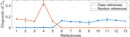
Figure 2: The average diagonal values of $\Sigma_{L}^{*}$ optimized for the first attribute of the OSR dataset as the target with remaining 5 attributes in the same dataset as references 1 to 5, plus 8 additional attributes as references 6 to 13. $\Sigma_{L}^{*}$ values are normalized to sum to one for visualization. The length of each error bar corresponds to twice the standard deviation. Class references: References 6–13 are class labels from which attribute labels are generated. Random references: References 6–13 are randomly generated. See text.

3.4 Joint denoising

So far, we assumed that all references in $\mathcal{G}$ are noise-free. However, in practice, they might be noisy estimates of the ground truth. In this case, noise in the references could be propagated to the target predictor during denoising, which would degrade the final output. We account for this by denoising all predictors $\mathcal{H}=\{\mathbf{f},\mathbf{g}_{1},\ldots,\mathbf{g}_{R}\}$ simultaneously. At each iteration $t$, each predictor $\mathbf{h}\in\mathcal{H}$ is denoised by considering it as the target predictor, and $\mathcal{H}\setminus\{\mathbf{h}\}$ as the references in Eq. 27. In the experiments with the OSR dataset, removing this joint denoising process from our final algorithm decreases the average accuracy rate by 8.26% (see Table 2). We provide a summary of our complete algorithm in the supplemental document.

Table 2: Effect of design choices in our algorithm on the OSR dataset. The average rank accuracy improvement over multiple target attributes from the baseline initial predictions $\mathbf{f}^{0}$ are shown (see Sec. 4 for details). w/o joint denois. only denoising the target predictor. w/o auto. relev.: without automatic relevance determination. Numbers in parentheses are accuracy ratios w.r.t. Final NPC.

Design choices $\to$	w/o joint denois.	w/o auto. relev.	Final NPC
Accuracy improvement	1.96 (91.74%)	1.88 (88.03%)	2.13 (100%)

Computational complexity and discussion. Assuming that $N\gg R$, the computational complexity of our algorithm (Eq. 27) is dominated by calculating the kernel matrix $K_{GB}$ (Eq. 14), which takes $O(NN^{\prime}R)$ for $N$ data points, $N^{\prime}$ basis vectors and $R$ references. The second-most demanding part is the calculation of $T^{\frac{1}{2}}$ from $T$ based on Cholesky decomposition (Eq. 15; $O(N^{\prime 3})$). As we denoise not only the target predictor but also all references, the overall computational complexity of each denoising step is $O(R\times(NN^{\prime}R+N^{\prime 3}))$. On a machine with an Intel Core i7 9700K CPU and an NVIDIA GeForce RTX 2080 Ti GPU, the entire denoising process, including optimization of $\{(\Sigma_{A})_{i}\}_{i=1}^{R}$ (Eq. 18), took around 10 seconds for the AWA2 dataset with 37,322 data points and 79 references for each target attribute. For simplicity, we use the low-rank approximation of $K$ (Eq. 14) for constructing sparse GP predictions, while more advanced methods exist [RasWill06]. The number $N^{\prime}$ of basis vectors is fixed at 300 throughout our experiments. While the accuracy of low-rank approximation (Eq. 14) is in general positively correlated with $N^{\prime}$, we have not observed any significant performance gain by raising $N^{\prime}$ to 1,000 in our experiments. GP predictions also generally improve when optimizing the basis matrix $B$, e.g. via the marginal likelihood [SnelGhah06] instead of being selected from datasets as we did. Our efficient eigenvector calculation approach (Eq. 17) can still be applied in these cases.

4 Experiments

We assessed the effectiveness of our predictor combination algorithm in two scenarios: 1) visual attribute ranking [ParGra11], and 2) multi-class classification guided by the estimated visual attribute ranks. Given a database of images $X\subset\mathcal{X}$, visual attribute ranking aims to introduce a linear ordering of entries in $X$ based on the strength of semantic attributes present in each image $\mathbf{x}\in X$. For a visual attribute, our goal is to estimate a rank predictor $f\colon\mathcal{X}\to\mathbb{R}$, such that $f(\mathbf{x}_{i})>f(\mathbf{x}_{j})$ when the attribute is stronger in $\mathbf{x}_{i}$ than $\mathbf{x}_{j}$. Parikh and Grauman’s original relative attributes algorithm [ParGra11] estimates a linear rank predictor $f(\mathbf{x})=\mathbf{w}^{\top}\mathbf{x}$ via rank SVMs that use the rank loss $\mathcal{L}$ defined on ground-truth ranked pairs $U\subset X\times X$:

$$\mathcal{E}(f) =\sum_{(\mathbf{x}_{i},\mathbf{x}_{j})\in U}\mathcal{L}(f,(\mathbf{x}_{i},\mathbf{x}_{j}))+C\|\mathbf{w}\|^{2}\text{,}$$ (19)

$$\mathcal{L}(f,(\mathbf{a},\mathbf{b})) =\max\left(1-(f(\mathbf{a})-f(\mathbf{b})),0\right)^{2}\text{.}$$ (20)

Yang et al. [YanZhaXu16] and Meng et al. [MenAdlKim18] extended this initial work using deep neural networks (neural rankers). Kim and Chang [KimCha19] extended the original predictor combination framework of Kim et al. [KimTomRic17] to rank predictor combination.

Experimental settings. For visual attribute ranking, we use seven datasets, each with annotations for multiple attributes per image. For each attribute, we construct an initial predictor and denoise it via predictor combination using the predictors constructed for the remaining attributes as the reference. The initial predictors are constructed by first training 1) neural rankers, 2) linear and 3) non-linear rank SVMs, and 4) semi-supervised rankers that use the iterated graph Laplacian-based regularizer [ZhoBelSre11], all using the rank loss $\mathcal{L}$ (Eq. 49). For each attribute, we select the ranker with the highest validation accuracy as baseline $\mathbf{f}^{0}=f|_{X}$.

We compare our proposed algorithm to: 1) the baseline predictor $\mathbf{f}^{0}$, 2) Kim and Chang’s adaptation [KimCha19] of Kim et al.’s predictor combination approach [KimTomRic17] to visual attribute ranking (OPC), and 3) Mejjati et al.’s multi-task learning (MTL) algorithm [MejCosKim18]. While the latter was originally designed for MTL problems, it does not require known forms of individual predictors and can be thus adapted for predictor combination. In the supplemental document, we also compare with an adaptation of Evgeniou et al.’s graph Laplacian-based MTL algorithm [EvgMicPon05] to the predictor combination setting, which demonstrates that all predictor combination algorithms outperform naïve adaptations of traditional MTL algorithms.

Adopting the experimental settings of Kim et al. [KimCha19, KimTomRic17], we tune the hyperparameters of all algorithms on evenly-split training and validation sets. Our algorithm requires tuning the noise level $\sigma^{2}$ (Eq. 28), global kernel scaling $\sigma_{k}^{2}$, and the regularization parameter $\lambda_{\text{J}}$ (Eq. 27), which are tuned based on validation accuracy. For the number of iterations $S$, we use 20 iterations and select the iteration number that achieves the highest validation accuracy. The hyperparameters for other algorithms are tuned similarly (see the supplemental material for details). For each dataset, we repeated experiments 10 times with different training, validation, and test set splits and report the average accuracies.

The OSR [ParGra11], Pubfig [ParGra11], and Shoes [KovParGra12] datasets provide 2688, 772 and 14,658 images each and include rank annotations (i.e. strengths of attributes present in images) for 6, 11 and 10 visual attributes, respectively. The attribute annotations in these datasets were obtained from the underlying class labels. For example, each image in OSR is also provided with a ground-truth class label out of 8 classes. The attribute ranking is assigned per class-wise comparisons such that all images in a class have stronger (or the same) presence of an attribute than another class. This implies that the class label assigned for each image completely determines its attributes, while attributes themselves might not provide sufficient information to determine classes. Similarly, the attribute annotations for Pubfig and Shoes are generated from class labels out of 8 and 10 classes, respectively. The input images in OSR and Shoes are represented as combinations of GIST [OlivaT2001] and color histogram features, while Pubfig uses GIST features as provided by the authors [KovParGra12, ParGra11]. In addition, for OSR, we extracted 2,048-dimensional features using ResNet101 pre-trained on ImageNet [HeZhaRen16] to fairly assess the predictor combination performance when the accuracies of the initial predictors are higher thanks to advanced features (OSR (ResNet)).

The aPascal dataset is constructed based on the Pascal VOC 2008 dataset [EveEslGoo15] containing 12,695 images with 64 attributes [FarEndHoi09]. Each image is represented as a 9,751-dimensional feature vector combining histograms of local texture, HOG, and edge and color descriptors. The Caltech-UCSD Birds-200-2011 (CUB) dataset [WaBraWelPerBel11] provides 11,788 images with 312 attributes where the images are represented by the ResNet101 features. The Animals With Attributes 2 (AWA2) dataset consists of 37,322 images with 85 attributes [XiaLamSch19]. We used the ResNet101 features as shared by Xian et al. [XiaLamSch19]. For aPascal, CUB, and AWA2, the distributions of attribute values are imbalanced. To ensure that sufficient numbers (300) of training and testing labels exist for each attribute level, we selected 29, 40 and 80 attributes from aPascal, CUB and AWA2, respectively. The ranking accuracy is measured in 100$\times$ Kendall’s rank correlation coefficient, which is defined as the difference between the numbers of correctly and incorrectly ordered rank pairs, respectively, normalized by the number of total pairs (bounded in $100\times[-1,1]$; higher is the better).

The UT Zappos50K (Zap50K) contains 50,025 images of shoes with 4 attributes. Each image is represented as a combination of GIST and color histogram features provided by Yu and Grauman [YuGra14]. The ground-truth attribute labels are collected by instance-level pairwise comparison collected via Mechanical Turk [YuGra14].

We also performed multi-class classification experiments on the OSR, Pubfig, Shoes, aPascal, and CUB datasets based on their respective class labels. The initial predictors $\mathbf{f}^{0}\colon\mathcal{X}\to\mathbb{R}^{H}$ are obtained as deep neural networks with continuous softmax decisions trained and validated on 20 labels per class. Each prediction is given as an $H$-dimensional vector with $H$ being the number of classes. Our goal is to improve $\mathbf{f}^{0}$ using the predictors for visual attribute ranking as references. It should be noted that our algorithm jointly improves all $H$ class-wise predictors as well as ranking references: 1) all class predictors evolve simultaneously, and 2) for improving the predictor of a class, the (evolving) predictors of the remaining classes are used as additional references. For a fair comparison, we denoise class-wise predictors using both the rank predictors and the predictors of the remaining classes as references, also for the other predictor combination algorithms.

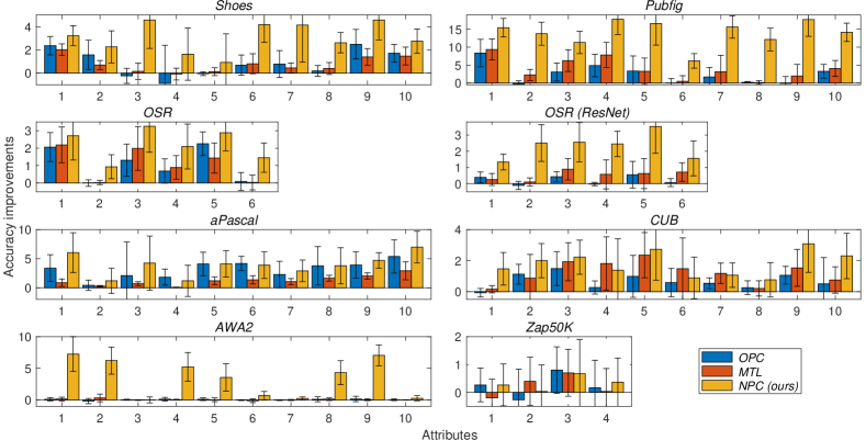
Figure 3: Average accuracy improvement of different predictor combination algorithms from the baseline predictors for up to first 10 attributes. The complete results including statistical significance tests can be found in the supplemental document.

Table 3: Average classification accuracies (%) using rank estimates as references. The numbers in parentheses show the relative accuracy improvement over the baseline $\mathbf{f}^{0}$.

	Shoes	Pubfig	OSR	aPascal	CUB
Baseline $\mathbf{f}^{0}$	57.90 (0.00)	77.99 (0.00)	76.88 (0.00)	37.86 (0.00)	66.98 (0.00)
OPC [KimCha19]	58.52 (1.07)	82.55 (5.85)	77.16 (0.38)	39.77 (5.04)	67.75 (1.15)
MTL [MejCosKim18]	59.51 (2.78)	80.16 (2.78)	77.40 (0.68)	38.38 (1.37)	67.95 (1.45)
NPC (ours)	62.87 (8.58)	86.51 (10.9)	79.71 (3.69)	40.34 (6.55)	68.26 (1.92)

Ranking results. Figure 3 summarizes the results for the relative attributes ranking experiments. Here, we show the results of only the first 10 attributes; the supplemental document contains complete results, which show a similar tendency as presented here. All three predictor combination algorithms frequently achieved significant performance gains over the baseline predictors $\mathbf{f}^{0}$. Importantly, apart from one case (Shoes attribute 4), all predictor combination algorithms did not significantly degrade the performance from the baseline. This demonstrates the utility of predictor combination. However, both OPC and MTL are limited in that they can only capture pairwise dependence between the target predictor and each reference. By taking into account the dependence present among the references, and thereby jointly exploiting them in improving the target predictor, our algorithm further significantly improves the performance: Our algorithm performs best for 87.1% of attributes. In particular, Ours showed significant improvement on 6 out of 10 AWA2 attributes, where the other algorithms achieved no noticeable performance gain. This supports our assumption that multiple attributes indeed can jointly supply relevant information for improving target predictors, even if not individually.

Multi-class classification results. Table 3 shows the results of improving multi-class classifications. Jointly capturing all rank predictors as well as the multi-dimensional classification predictions as references, our algorithm demonstrates significant performance gains (especially on Shoes and Pubfig), while other predictor combination algorithms achieved only marginal improvements, confirming the effectiveness of our joint prediction strategy.

5 Discussions and Conclusions

Our algorithm builds upon the assumption that the reference predictors can help improve the target predictor when they can well predict (or explain) the ground-truth $\mathbf{f}_{\text{GT}}$. Since $\mathbf{f}_{\text{GT}}$ is not available during testing, we use the noisy target predictor $\mathbf{f}^{t}$ at each time step $t$ as a surrogate, which by itself is iteratively denoised. While our experiments demonstrate the effectiveness of this approach in real-world examples, simple failure cases exist. For example, if $\mathbf{f}^{0}$ (as the initial surrogate to $\mathbf{f}_{\text{GT}}$) is contained in the reference set $\mathcal{G}$, our automatic reference determination approach will pick this up as the single most relevant reference, and therefore, the resulting predictor combination process will simply output $\mathbf{f}^{0}$ as the final result. We further empirically observed that even when the automatic relevance determination is disabled (i.e. $\Sigma_{L}=I$), the performance degraded significantly when $\mathbf{f}^{0}$ is included in $\mathcal{G}$. Also, as shown for the Zap50K results, there might be cases where no algorithm shows any significant improvement (indicated by the relatively large error bars). In general, our algorithm may fail when the references do not communicate sufficient information for improving the target predictor. Quantifying such utility of references and predicting the failure cases may require a new theoretical analysis framework.

Existing predictor combination algorithms only consider pairwise relationships between the target predictor and each reference. This misses potentially relevant information present in the dependence among the references. We explicitly address this limitation by introducing a new predictability criterion that measures how references are jointly contributing in predicting the target predictor. Adopting a fully Bayesian framework, our algorithm can automatically select informative references among many potentially irrelevant predictors. Experiments on seven datasets demonstrated the effectiveness of the proposed predictor combination algorithm.

Acknowledgements. This work was supported by UNIST’s 2020 Research Fund (1.200033.01), National Research Foundation of Korea (NRF) grant NRF-2019R1F1A1061603, and Institute of Information & Communications Technology Planning & Evaluation (IITP) grant (No.20200013360011001, Artificial Intelligence Graduate School support (UNIST)) funded by the Korean government (MSIT).

Supplemental Document for
Combining Task Predictors
via Enhancing Joint Predictability

In this supplemental document, we present:

1. Details of the marginal likelihood calculation used in the automatic determination of relevant predictors $\Sigma_{L}$ (Sec. 6.1);

2. A summary of our predictor combination algorithm (Sec. 6.2);

3. A detailed discussion of baseline algorithms, including:

   1. our adaptation of Mejjati et al.’s multi-task learning (MTL) algorithm [MejCosKim18] (Sec. 7.1),

   2. a derivation of Kim et al.’s original predictor combination (OPC) algorithm [KimTomRic17, KimCha19] (Sec. 7.2), and

   3. Evgeniou et al.’s graph Laplacian (GL)-based MTL algorithm and its adaptation to predictor combination (Sec. 7.3).

In the main paper, we only presented the ranking results for the first 10 attributes in each dataset. In Section 8, we provide the complete experimental results, including additional results of GL and tests of statistical significance of the accuracy improvements made by different algorithms. We reproduce some content from the main paper to make this document self-contained.

6 Details of the main algorithm

6.1 Calculating the marginal likelihood for linear Gaussian process prediction

Suppose that we have the following linear and nonlinear anisotropic covariance functions:

$$k_{L}(\mathbf{a},\mathbf{b}) =\mathbf{a}^{\top}\Sigma_{L}\mathbf{b}\text{,}$$ (21)

$$k_{A}(\mathbf{a},\mathbf{b}) =\exp\left(-(\mathbf{a}-\mathbf{b})^{\top}\Sigma_{A}(\mathbf{a}-\mathbf{b})\right)\text{,}$$ (22)

where $\Sigma_{L}=\operatorname{diag}[\bm{\sigma}]$, the diagonal matrix with elements $\bm{\sigma}=[\sigma^{1},\ldots,\sigma^{n}]^{\top}$. $\Sigma_{A}$ is defined similarly. Our goal is to maximize the marginal likelihood $p(\mathbf{f}\mid G,\Sigma_{L})$ of the sampled predictor $\mathbf{f}$ given the reference matrix $G$ with respect to $\bm{\sigma}$. The log marginal likelihood $\log(p(\mathbf{f}\mid G,\Sigma_{L}))$ of linear Bayesian regression with Gaussian prior and i.i.d. Gaussian noise model is given as [RasWill06]:

$$\log(p(\mathbf{f}\mid G))= -\frac{1}{2}\log\left|G\cdot\operatorname{diag}[\bm{\sigma}]\cdot G^{\top}+\lambda I\right|-\frac{N}{2}\log(2\pi)$$

$$-\frac{1}{2}\mathbf{f}^{\top}(G\cdot\operatorname{diag}[\bm{\sigma}]\cdot G^{\top}+\lambda I)^{-1}\mathbf{f}\text{.}$$ (23)

As maximizing $p(\mathbf{f}\mid G,\Sigma_{L})$ is equivalent to minimizing $-\log(p(\mathbf{f}\mid G,\Sigma_{L}))$, and the second term in $\log(p(\mathbf{f}\mid G,\Sigma_{L}))$ is independent of $\bm{\sigma}$, we can find the optimal parameter vector $\bm{\sigma}^{*}$ by minimizing the following energy:

$$\mathcal{E}(\bm{\sigma})= \log\left|G\cdot\operatorname{diag}[\bm{\sigma}]\cdot G^{\top}+\lambda I\right|+\mathbf{f}^{\top}(G\cdot\operatorname{diag}[\bm{\sigma}]\cdot G^{\top}+\lambda I)^{-1}\mathbf{f}$$ (24)

$$= N\log\left|\lambda\right|+\sum_{i=1}^{n}\log(\sigma^{i})+\log\left|\operatorname{diag}[1./\bm{\sigma}]+G^{\top}G/\lambda\right|$$

$$+\mathbf{f}^{\top}\left(\frac{1}{\lambda}I-\frac{1}{\lambda^{2}}G\left(\operatorname{diag}[1./\bm{\sigma}]+\frac{1}{\lambda}G^{\top}G\right)^{-1}G^{\top}\right)\mathbf{f}\text{,}$$

where the second equation is obtained by applying the Sherman–Morrison–Woodbury formula [SheMor50] to both summands of $\mathcal{E}$, and ‘$1./\bm{\sigma}$’ is the element-wise reciprocal of $\bm{\sigma}$. Since $\frac{1}{\lambda}\mathbf{f}^{\top}\mathbf{f}$ and $N\log\left|\lambda\right|$ are also independent of $\bm{\sigma}$, minimizing $\mathcal{E}$ is equivalent to minimizing

$$\mathcal{E}^{\prime}(\bm{\sigma})= \sum_{i=1}^{n}\log(\sigma^{i})+\log\left|\operatorname{diag}[1./\bm{\sigma}]+G^{\top}G/\lambda\right|$$ (25)

$$-\frac{1}{\lambda^{2}}\mathbf{f}^{\top}\left(G\left(\operatorname{diag}[1./\bm{\sigma}]+\frac{1}{\lambda}G^{\top}G\right)^{-1}G^{\top}\right)\mathbf{f}\text{.}$$

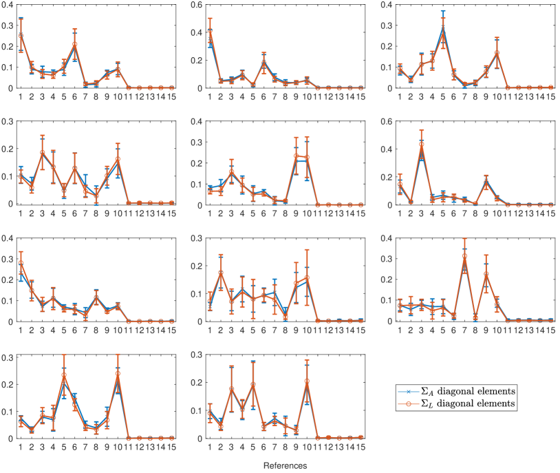
Figure 4: The average diagonal values of $\Sigma_{A}$ and $\Sigma_{L}$ optimized for each attribute in the Pubfig dataset as the target with the remaining 10 attributes in the same dataset (references 1 to 10), plus 5 additional randomly generated attributes (references 11 to 15) as references. The values of $\Sigma_{A}$ and $\Sigma_{L}$ are normalized such that the respective sums total to one. Note that the unrelated references (11–15) are correctly detected as irrelevant (small magnitudes and standard deviations) and hence ignored. In addition, the linear kernel $\Sigma_{L}$ (orange) is highly correlated to the anisotropic kernel $\Sigma_{A}$ (blue), so we use a scaled version of $\Sigma_{L}$ as a surrogate to the optimal $\Sigma_{A}^{*}$ (Eq. 26).

Since this energy $\mathcal{E}^{\prime}$ is a continuously differentiable function of $\bm{\sigma}$, it can be minimized by standard gradient descent. Figure 4 shows example parameters $\bm{\sigma}^{*}$ optimized for the Pubfig dataset. For each of the 11 attributes in Pubfig as a target, we optimized the corresponding parameters $\bm{\sigma}$ using the remaining attributes as references, plus 5 additional randomly generated references. As indicated by small magnitudes and the corresponding standard deviations of the $\bm{\sigma}^{*}$ entries, our algorithm successfully disregards these irrelevant references. For comparison, we also show the corresponding parameters optimized for the anisotropic Gaussian kernel $k_{A}$ (Eq. 22), demonstrating that once normalized, their relative scaling behaviors are similar, i.e.

$$\Sigma_{A}^{*}\approx\frac{\Sigma_{L}^{*}}{\sigma_{k}^{2}}$$ (26)

for a global scaling parameter $\sigma_{k}^{2}$. Our final algorithm uses $\Sigma_{L}^{*}/\sigma_{k}^{2}$ as a surrogate to $\Sigma_{A}^{*}$, using $\sigma_{k}^{2}$ as hyperparameter.

6.2 Algorithm summary

Given the reference matrix $G$, the initial predictor $\mathbf{f}^{0}$, and hyperparameters (noise variance $\sigma^{2}$ in Eq. 28; global kernel scaling $\sigma^{2}_{k}$ in Eq. 26; regularization parameter $\lambda_{\text{J}}$ in Eq. 27), our algorithm constructs a denoised predictor by iteratively maximizing the objective

$$\mathcal{O}_{\text{N}}(\mathbf{f})= \frac{\mathbf{f}^{\top}A\mathbf{f}}{\mathbf{f}^{\top}C_{N}\mathbf{f}}\quad\text{with}$$ (27)

$$A= (C_{N}\mathbf{f}^{t})(C_{N}\mathbf{f}^{t})^{\top}+\lambda_{\text{J}}Q^{\prime}\quad\text{and}$$

$$Q^{\prime}= C_{N}(2K(K+\sigma^{2}I)^{-1}-(K+\sigma^{2}I)^{-1}KK(K+\sigma^{2}I)^{-1})C_{N}\text{.}$$ (28)

Algorithm 1 summarizes this process.

Algorithm 1 Nonlinear predictor combination

1:Initial predictor $\mathbf{f}^{0}$, references $\{\mathbf{g}_{i}\}_{i=1}^{R}$, noise variance $\sigma^{2}$ (Eq. 28), global kernel scaling $\sigma^{2}_{k}$, regularization parameter $\lambda_{\text{J}}$ (Eq. 27), and iteration number $S$.

2:$\mathcal{H}^{0}=\{\mathbf{h}_{0}^{0},\mathbf{h}_{1}^{0},\ldots,\mathbf{h}_{R}^{0}\}\Leftarrow\{\mathbf{f}^{0},\mathbf{g}_{1},\ldots,\mathbf{g}_{R}\}$;

3:Calculate the kernel parameter matrix $(\Sigma_{L}^{*})_{i}$ for each $\mathbf{h}_{i}^{0}\in\mathcal{H}^{0}$; $(\Sigma_{A})_{i}=(\Sigma_{L}^{*})_{i}/\sigma^{2}_{k}$;

4:for step $t\in\{0,\ldots,S-1\}$ do

5:   for reference $i\in\{0,\ldots,R\}$ do

6:      Calculate $\mathbf{h}_{i}^{t+1}\in\mathcal{H}^{t+1}$ by maximizing $\mathcal{O}_{\text{N}}$ based on $\mathcal{H}^{t}$ (Eq. 27);

7:   end for

8:end for

9:Denoised target predictor $\mathbf{f}^{*}=\mathbf{h}_{0}^{S}$.

7 (Adapting) Existing algorithms

7.1 Mejjati et al.’s MTL algorithm

Mejjati et al.’s MTL algorithm considers each task-specific predictor as a random variable. Then, the relationships between tasks are modeled based on the statistical dependence estimated by evaluating these predictor random variables on a dataset $X$ [MejCosKim18]. Adopting a nonparametric measure of statistical dependence, the finite set independence criterion (FSIC) [JitSzaGre15], MTL enables training multiple predictors independently of their parametric forms and, therefore, it can be applied to predictor combination problems.

Applying this algorithm to the predictor combination setting, we construct the initial predictor matrix $H^{0}$ by stacking column-wise, the initial target predictor $\mathbf{f}^{0}$ and the references $\{\mathbf{g}_{1},\ldots,\mathbf{g}_{R}\}$

$$H^{0}=[\mathbf{f}^{0},\mathbf{g}_{1},\ldots,\mathbf{g}_{R}]\text{.}$$ (29)

MTL then refines the initial predictor matrix $H^{0}$ by minimizing the energy

$$\mathcal{E}_{\text{M}}(H)= \left\|H-H^{0}\right\|^{2}_{\text{F}}-\lambda_{1}\left\|\operatorname{vec}(\Phi(H))\right\|_{2}^{2}+\lambda_{2}\left\|\operatorname{vec}(\Phi(H))\right\|_{1}\text{,}$$ (30)

where $\operatorname{vec}(A)$ constructs a vector by concatenating columns of matrix $A$, $\Phi(H)$ is an $(R+1)\times(R+1)$-sized matrix consisting of pairwise FSIC evaluations: $\Phi(H)_{[i,j]}$ takes a large positive value when $H_{[:,i]}$ and $H_{[:,j]}$ exhibit strong statistical dependence and it takes 0 when $H_{[:,i]}$ and $H_{[:,j]}$ are independent as realizations of random variables. Minimizing $\mathcal{E}_{\text{M}}$ strengthens overall task dependence via (negation of) the $L^{2}$ norm of $\operatorname{vec}(\Phi(H))$ and, at the same time, introduces sparsity in the task dependence via the $L^{1}$ norm of $\Phi(H)$. Combing these two terms, MTL selectively enforces task dependence while suppressing the dependence of weakly related tasks as outliers. As $\mathcal{E}_{\text{M}}$ is not differentiable, standard gradient-descent type algorithms are not applicable. Instead, it is minimized based on the alternating direction method of multipliers (ADMM) approach. This involves iteratively solving ADMM sub-problems [BoyParChu10], with the number of total iterations $S$ as a hyperparameter. Once the optimal predictor matrix $H^{*}$ is constructed, the final denoised predictor is obtained by extracting the first column of $H^{*}$: $\mathbf{f}^{*}=H^{*}_{[:,1]}$. Similarly to our algorithm, $S$ is determined by setting the maximum number of iterations at 50 and selecting the iteration number achieving the highest validation accuracy. The other two hyperparameters, $\lambda_{1}$ and $\lambda_{2}$, are tuned based on validation accuracy.

7.2 Derivation of Kim et al.’s algorithm (OPC).

Kim et al.’s original predictor combination (OPC) approach iteratively minimizes the following energy (Eq. 1 in the main paper):

$$\mathcal{E}_{\text{O}}(f) =D_{\text{KL}}(f\mid f^{t})^{2}+\lambda_{\text{O}}\sum_{i=1}^{R}w_{i}D_{\text{KL}}(f\mid g_{i})^{2}\text{,}$$ (31)

$$w_{i} =\exp\left(-\frac{D_{\text{KL}}(f^{t}\mid g_{i})^{2}}{\sigma^{2}_{\text{O}}}\right)\text{,}$$ (32)

with $\lambda_{\text{O}},\sigma^{2}_{\text{O}}>0$ being hyperparameters. We present how this algorithm is obtained as an instance of Hein and Maier’s Manifold Denoising algorithm [HeiMai07] by discretizing a diffusion process on a predictor manifold $\mathcal{M}$.

Manifold denoising [HeiMai07].

Suppose that we have a set of data points $\mathcal{H}^{0}=\{\mathbf{h}^{0}_{i}\}_{i=1}^{n}$ presented as a sample from a Euclidean space $\mathbb{R}^{d}$ and, further, that the points in $\mathcal{H}^{0}$ are sampled from an underlying data-generating manifold $\mathcal{M}$ embedded in $\mathbb{R}^{d}$ ($\imath(\mathcal{M})\subset\mathbb{R}^{d}$ with $\imath$ being the embedding), and they are observed as a subset of $\mathbb{R}^{d}$ contaminated with i.i.d. Gaussian noise $\bm{\epsilon}$ in $\mathbb{R}^{d}$:

$$\mathbf{h}_{i}^{0}=\imath(\widetilde{\mathbf{h}}_{i}^{0})+\bm{\epsilon}\in\mathbb{R}^{d}\quad\text{for}\quad\widetilde{\mathbf{h}}_{i}^{0}\in\mathcal{M}\text{.}$$ (33)

The manifold denoising algorithm denoises $\mathcal{H}^{0}$ by simulating diffusion on a graph $G$ that discretizes $\mathcal{M}$ (each point $\mathbf{h}_{i}^{0}\in\mathcal{H}^{0}$ forms a vertex of $G$):

$$\frac{\partial H}{\partial t}=-\delta LH\text{,}$$ (34)

where $H=[\mathbf{h}_{1},\ldots,\mathbf{h}_{n}]^{\top}$ and $L$ is the graph Laplacian:

$$L =I-D^{-1}W\text{,}$$ (35)

$$W_{[i,j]} =\exp\left(-\frac{\left\|\mathbf{h}_{i}-\mathbf{h}_{j}\right\|^{2}}{\sigma^{2}}\right)\text{,}$$ (36)

and $D$ is a diagonal matrix consisting of row sums of $W$, such that $D_{ii}=\sum_{j=1}W_{[i,j]}$. Now discretizing Eq. 34 using the implicit Euler method, we obtain

$$H^{t+1}-H^{t}=-\delta LH^{t+1}\text{.}$$ (37)

At each time step $t$, the solution $H^{t+1}$ of Eq. 37 is obtained as the minimizer of the following energy:

$$\mathcal{E}_{\text{D}}(H)=\left\|H-H^{t}\right\|_{\text{F}}^{2}+\delta\mathop{\rm tr}\nolimits[H^{\top}LH]\text{,}$$ (38)

where $\left\|A\right\|_{\text{F}}$ and $\mathop{\rm tr}\nolimits[A]$ are the Frobenius norm and trace of matrix $A$, respectively. As the number of data points $n$ grows to infinity, $G$ becomes a precise representation of $\mathcal{M}$ embedded in $\mathbb{R}^{d}$, and $L$ converges to the Laplace-Beltrami operator $\Delta_{\mathcal{M}}$ on $\mathcal{M}$ casting Eq. 37 into a diffusion process on a continuous manifold $\mathcal{M}$ [HeiMai07]. It should be noted that the graph Laplacian was constructed based on the ambient $L^{2}$ distance in $\mathbb{R}^{d}$ rather than the intrinsic metric on $\mathcal{M}$. This facilitates building a practical, still consistent algorithm: Equation 38 only requires the ambient Euclidean distance (via $L$) without having to access $\mathcal{M}$ directly, but it guarantees the statistical consistency of $L$ as proven by Hein and Maier [HeiMai07].

Now applying this algorithm to the predictor combination setting and, therefore, assuming that only the first point $\mathbf{h}_{1}^{0}\in\mathcal{H}^{0}$ is noisy (i.e. $\mathbf{h}_{i}=\imath(\tilde{\mathbf{h}}_{i})$ for $i=\{2,\ldots,n\}$), we obtain an iterative update rule of $\mathbf{h}_{1}^{t}$ given fixed references $\{\mathbf{h}_{i}\}_{i=2}^{n}$:

$$\mathcal{E}_{\text{D}}(\mathbf{h})=\left\|\mathbf{h}-\mathbf{h}_{1}^{t}\right\|^{2}+\delta\sum_{i=2}^{n}W_{[1,i]}\left\|\mathbf{h}-\mathbf{h}_{i}\right\|^{2}\text{.}$$ (39)

Finally, $\mathcal{E}_{\text{O}}$ in Eq. 31 is obtained by replacing each point in $\mathcal{H}^{t}$ and the corresponding $L^{2}$ distances in $\mathcal{E}_{\text{D}}$ with a Gaussian process predictor and Kullback–Leibler divergences, respectively: $\mathbf{h}_{1}^{t}$ and $\{\mathbf{h}_{i}\}_{i=2}^{n}$ (with $n=R+1$) are considered as the target predictor $\mathbf{f}$ and the corresponding references $\{\mathbf{g}_{i}\}$, respectively.

7.3 Evgeniou et al.’s graph Laplacian (GL)-based MTL algorithm.

Evgeniou et al.’s graph Laplacian (GL)-based algorithm learns predictors $\mathcal{H}=\{h_{i}\}_{i=1}^{n}$ of multiple tasks by enforcing pairwise parameter similarities: Assuming that all predictors are linear, i.e. $h_{i}(\mathbf{x})=\mathbf{w}_{i}^{\top}\mathbf{x}$, their algorithm estimates the predictor parameters $W=\{\mathbf{w}_{1},\ldots,\mathbf{w}_{n}\}$ by minimizing the energy

$$\mathcal{E}_{\text{GL}}(W)= \sum_{i=1}^{n}l_{i}(h_{i})+\lambda_{1}\sum_{i=1}^{n}\left\|\mathbf{w}_{i}\right\|^{2}+\lambda_{2}\sum_{i=1}^{n}\sum_{j\neq i}U_{[i,j]}\left\|\mathbf{w}_{i}-\mathbf{w}_{j}\right\|^{2}\text{,}$$ (40)

where $\{l_{i}(\cdot)\}_{i=1}^{n}$ are task-specific loss functions and $U_{[i,j]}\geq 0$ represents the relationship between tasks $i$ and $j$. Now adapting this algorithm to the predictor combination setting, we assume that the initial predictor $f^{0}=h_{1}$ and the corresponding references $g_{i}=h_{i+1}$ for $i\in\{1,\ldots,R\}$ are given ($n=R+1$). Then, $f^{0}$ is refined by minimizing the energy

$$\mathcal{E}_{\text{GL}}(\mathbf{w}) =\left\|\mathbf{w}-\mathbf{w}_{1}^{0}\right\|^{2}+\lambda_{\text{GL}}\sum_{j=2}^{n}U_{[1,j]}\left\|\mathbf{w}-\mathbf{w}_{j}\right\|^{2}\text{.}$$ (41)

In general, determining the task relationship parameters $\{U_{[1,j]}\}$ is a challenging problem. Here, we determine them by adopting Kim et al.’s approach: We iteratively update $\{U_{[1,j]}\}$ by minimizing $\mathcal{E}_{\text{GL}}$ at each time step $t$ with

$$U_{[1,j]} =\exp\left(-\frac{\left\|\mathbf{w}_{i}-\mathbf{w}_{1}^{t}\right\|^{2}}{\sigma_{\text{GL}}^{2}}\right)\text{.}$$ (42)

Further, adopting Kim and Chang’s approach [KimCha19], we explicitly constrain all predictor parameter vectors to have unit norm: $\left\|\mathbf{w}_{i}\right\|=1$, enabling the comparison of task predictor parameters independently of their scales. The two hyperparameters $\sigma_{\text{GL}}^{2}$ and $\lambda_{\text{GL}}$ are determined based on validation accuracy. As often, ranking problems are nonlinear, we extend this framework by adopting the linear-in-parameter model:

$$f(\mathbf{x})=\phi(\mathbf{x})^{\top}\mathbf{w}_{f}\text{,}$$ (43)

where $\phi\colon\mathcal{X}\to\mathcal{F}_{k}$ with $\mathcal{F}_{k}$ being the reproducing kernel Hilbert space (RKHS) corresponding to a Gaussian kernel with hyperparameter $\sigma_{k}^{2}$ [Sch02]:

$$k(\mathbf{a},\mathbf{b})=\exp\left(-\frac{\left\|\mathbf{a}-\mathbf{b}\right\|^{2}}{\sigma_{k}^{2}}\right)\text{.}$$ (44)

In this case, the target predictor $f$ is represented based the original parameter vector $\mathbf{w}_{f}$ as well as its dual parameter vector $\mathbf{a}_{f}=[a^{1}_{f},\ldots,a^{N^{\prime}}_{f}]^{\top}$:

$$f(\mathbf{x}):=\phi(\mathbf{x})^{\top}\mathbf{w}_{f}=\sum_{j=1}^{N^{\prime}}a_{f}^{j}k(\mathbf{b}_{j},\mathbf{x})\text{,}$$ (45)

with $\{\mathbf{b}_{i}\}_{i=1}^{N^{\prime}}$ being a set of basis vectors. The reference predictors $\{g_{i}\}_{i=1}^{R}$ are represented similarly:

$$g_{i}(\mathbf{x}):=\phi(\mathbf{x})^{\top}\mathbf{w}_{i}=\sum_{j=1}^{N^{\prime}}a_{i}^{j}k(\mathbf{b}_{j},\mathbf{x})\text{.}$$ (46)

Under this setting, the parameter similarity $\left\|\mathbf{w}_{f}-\mathbf{w}_{i}\right\|$ can be calculated using the standard kernel trick [Sch02] as

$$\left\|\mathbf{w}_{f}-\mathbf{w}_{j}\right\|=\mathbf{a}_{f}^{\top}K\mathbf{a}_{f}^{\top}+\mathbf{a}_{i}^{\top}K\mathbf{a}_{i}^{\top}-2\mathbf{a}_{f}^{\top}K\mathbf{a}_{i}^{\top}\text{,}$$ (47)

with $K_{[i,j]}=k(\mathbf{b}_{i},\mathbf{b}_{j})$. It should be noted that efficient calculation of $\|\mathbf{w}_{f}-\mathbf{w}_{i}\|$ based on Eq. 47 requires that all predictors should share the same RKHS determined by the kernel parameter $\sigma_{k}$. To facilitate this, in our experiments, we first determine $f^{0}$ as nonlinear rank support vector machine that minimizes the regularized energy

$$\mathcal{E}_{\text{S}}(f) =\sum_{(\mathbf{x}_{i},\mathbf{x}_{j})\in U}\mathcal{L}(f,(\mathbf{x}_{i},\mathbf{x}_{j}))+C_{f}\|\mathbf{w}\|^{2}\text{,}$$ (48)

$$\mathcal{L}(f,(\mathbf{a},\mathbf{b})) =\max\left(1-(f(\mathbf{a})-f(\mathbf{b})),0\right)^{2}$$ (49)

for the rank loss $\mathcal{L}$ defined on ground-truth ranked pairs $U\subset X\times X$ and tune the hyperparameters $\sigma^{2}_{k}$ and $C_{f}$ based on validation accuracy. Once $f^{0}$ is fixed in this way, the reference predictors $\{g_{i}\}_{i=1}^{R}$ are determined by minimizing $\mathcal{E}_{\text{S}}$ for the respective rank labels. However, for these references, only the respective regularization hyperparameters $\{C_{i}\}_{i=1}^{R}$ are tuned while the corresponding kernel parameters are all fixed as $\sigma^{2}_{k}$ (optimized for $f^{0}$), to facilitate the computation of $\left\|\mathbf{w}-\mathbf{w}_{i}\right\|$ (Eq. 47). We fixed $N^{\prime}$ at 500 and selected the basis vectors $\{\mathbf{b}_{i}\}_{i=1}^{N^{\prime}}$ as the cluster centers of input data points $X$, estimated using $k$-means clustering.

Note that this setting violates the application conditions of predictor combination: It requires access to the forms of all predictors $\{f,g_{1},\ldots,g_{R}\}$ and, further, it assumes that all predictors share the same form (Eqs. 45 and 46). We show in Sec. 8 that the latter homogeneity requirement poses a severe limitation on predictor combination performance. Even when GL took advantage of known predictor forms, except for a few cases, the other predictor combination algorithms significantly outperformed GL. Often, the results of GL are even worse than the initial predictors $\mathbf{f}^{0}$ that are obtained by selecting the best predictors (via validation) from the heterogeneous predictor pools.

8 Complete ranking results

Table 4 summarizes the results for the relative attributes ranking experiments (see Tables 5–9 for complete results). Our algorithm NPC performs best for 87% (162/186) of attributes. In particular, it showed statistically significant improvement on 74 out of 80 AWA2 attributes, while the baselines OPC and MTL achieved significant performance gains only on 8 and 33 attributes, respectively.

Overall, our algorithm NPC is often statistically significantly better than these methods and – apart from only one attribute (for CUB) out of 186 – ours is not statistically significantly worse than the other methods. This demonstrates that the baselines OPC and MTL are limited in that they can only capture pairwise dependence between the target predictor and each reference. Taking into account the dependence present among the references, and thereby jointly exploiting them in improving the target predictor, our algorithm NPC (Ours) significantly improves the performance.

Table 4: A summary of the results of statistical significance tests of our method NPC compared to baseline $\mathbf{f}^{0}$, GL, OPC and MTL, based on a t–test with $\alpha=0.95$. For each method, we show #attributes where our NPC is statistically significantly better (first column), on par with (second column), and statistically significantly worse (third column).

Dataset	vs. baseline $\mathbf{f}^{0}$			vs. GL			vs. OPC			vs. MTL			# total attr.
Shoes	9	1	0	10	0	0	8	2	0	9	1	0	10
Pubfig	11	0	0	11	0	0	11	0	0	11	0	0	11
OSR	6	0	0	2	4	0	4	2	0	5	1	0	6
OSR (ResNet)	6	0	0	6	0	0	6	0	0	6	0	0	6
aPascal	25	4	0	16	13	0	9	20	0	19	10	0	29
CUB	31	9	0	23	17	0	26	14	0	12	27	1	40
AWA2	74	6	0	73	7	0	71	9	0	72	8	0	80
Zap50K	0	4	0	0	4	0	0	4	0	0	4	0	4
# total attr.	162	24	0	141	45	0	135	51	0	134	51	1	186

Table 5: Ranking accuracies of different predictor combination algorithms on the Shoes, Pubfig, OSR, and OSR (ResNet) datasets. For each dataset, we repeated experiments 10 times with different training, validation, and test set splits. For baseline $\mathbf{f}^{0}$ (second column), Kendall’s Tau correlations$\times$100 (standard deviations in parentheses) are presented. For the remaining algorithms (third to sixth columns), the accuracy offsets from $\mathbf{f}^{0}$ are presented. The best and second best results are highlighted with bold and italic fonts, respectively. The results of statistical significance test based on a t–test with $\alpha=0.95$ are highlighted in green (significantly positive) and orange (significantly negative). The last three columns show the results of statistical significance test of our algorithm with GL, OPC, and MTL, respectively (${\color[rgb]{0,1,0}{+}}$/${\color[rgb]{1,0.23,0.13}{-}}$: significantly positive/negative).

Shoes
Attr.	Baseline $\mathbf{f}^{0}$	GL	OPC	MTL	NPC (ours)	vs. GL	vs. OPC	vs. MTL
1	72.09 (1.71)	-0.36 (1.44)	2.36 (0.79)	2.03 (0.49)	3.21 (0.86)	${\color[rgb]{0,1,0}{+}}$	${\color[rgb]{0,1,0}{+}}$	${\color[rgb]{0,1,0}{+}}$
2	63.84 (1.87)	-2.04 (2.94)	1.57 (1.25)	0.70 (0.39)	2.26 (1.38)	${\color[rgb]{0,1,0}{+}}$	$0$	${\color[rgb]{0,1,0}{+}}$
3	38.07 (2.11)	-1.38 (2.43)	-0.24 (0.65)	0.16 (0.70)	4.58 (2.45)	${\color[rgb]{0,1,0}{+}}$	${\color[rgb]{0,1,0}{+}}$	${\color[rgb]{0,1,0}{+}}$
4	50.10 (2.75)	-2.45 (2.59)	-0.88 (3.29)	-0.08 (0.51)	1.63 (2.25)	${\color[rgb]{0,1,0}{+}}$	${\color[rgb]{0,1,0}{+}}$	${\color[rgb]{0,1,0}{+}}$
5	65.76 (1.20)	-1.11 (1.84)	-0.05 (0.16)	0.13 (0.34)	0.92 (2.46)	${\color[rgb]{0,1,0}{+}}$	$0$	$0$
6	65.02 (1.83)	-0.86 (1.13)	0.68 (0.87)	0.81 (0.86)	4.18 (1.54)	${\color[rgb]{0,1,0}{+}}$	${\color[rgb]{0,1,0}{+}}$	${\color[rgb]{0,1,0}{+}}$
7	59.38 (2.06)	-3.31 (1.59)	0.78 (1.16)	0.45 (0.42)	4.14 (3.20)	${\color[rgb]{0,1,0}{+}}$	${\color[rgb]{0,1,0}{+}}$	${\color[rgb]{0,1,0}{+}}$
8	56.85 (2.04)	-2.57 (1.46)	0.19 (0.46)	0.40 (0.51)	2.62 (0.87)	${\color[rgb]{0,1,0}{+}}$	${\color[rgb]{0,1,0}{+}}$	${\color[rgb]{0,1,0}{+}}$
9	65.15 (1.94)	0.35 (1.94)	2.49 (1.27)	1.40 (0.72)	4.58 (1.72)	${\color[rgb]{0,1,0}{+}}$	${\color[rgb]{0,1,0}{+}}$	${\color[rgb]{0,1,0}{+}}$
10	72.10 (1.24)	-1.26 (1.55)	1.71 (0.77)	1.47 (0.77)	2.75 (1.05)	${\color[rgb]{0,1,0}{+}}$	${\color[rgb]{0,1,0}{+}}$	${\color[rgb]{0,1,0}{+}}$
Pubfig
Attr.	Baseline $\mathbf{f}^{0}$	GL	OPC	MTL	NPC (ours)	vs. GL	vs. OPC	vs. MTL
1	67.13 (2.75)	4.89 (2.48)	8.37 (3.84)	9.37 (2.94)	15.45 (2.59)	${\color[rgb]{0,1,0}{+}}$	${\color[rgb]{0,1,0}{+}}$	${\color[rgb]{0,1,0}{+}}$
2	62.49 (2.41)	-0.96 (2.62)	-0.31 (0.91)	2.24 (1.55)	13.78 (3.23)	${\color[rgb]{0,1,0}{+}}$	${\color[rgb]{0,1,0}{+}}$	${\color[rgb]{0,1,0}{+}}$
3	68.31 (2.33)	2.27 (3.27)	3.06 (2.52)	6.25 (3.04)	11.33 (3.10)	${\color[rgb]{0,1,0}{+}}$	${\color[rgb]{0,1,0}{+}}$	${\color[rgb]{0,1,0}{+}}$
4	63.98 (3.46)	8.44 (4.26)	4.88 (3.14)	7.84 (3.49)	17.80 (4.26)	${\color[rgb]{0,1,0}{+}}$	${\color[rgb]{0,1,0}{+}}$	${\color[rgb]{0,1,0}{+}}$
5	61.27 (2.96)	6.15 (2.92)	3.33 (4.23)	3.26 (3.70)	16.62 (6.02)	${\color[rgb]{0,1,0}{+}}$	${\color[rgb]{0,1,0}{+}}$	${\color[rgb]{0,1,0}{+}}$
6	81.60 (1.26)	-1.09 (2.67)	-0.03 (1.25)	0.44 (1.58)	6.17 (2.03)	${\color[rgb]{0,1,0}{+}}$	${\color[rgb]{0,1,0}{+}}$	${\color[rgb]{0,1,0}{+}}$
7	64.23 (2.88)	2.87 (3.13)	1.68 (2.67)	3.14 (4.61)	15.66 (3.14)	${\color[rgb]{0,1,0}{+}}$	${\color[rgb]{0,1,0}{+}}$	${\color[rgb]{0,1,0}{+}}$
8	66.10 (3.53)	0.38 (2.66)	0.19 (0.21)	0.10 (0.49)	12.16 (3.17)	${\color[rgb]{0,1,0}{+}}$	${\color[rgb]{0,1,0}{+}}$	${\color[rgb]{0,1,0}{+}}$
9	59.73 (4.79)	3.58 (3.78)	-0.11 (1.89)	1.96 (3.20)	17.74 (4.68)	${\color[rgb]{0,1,0}{+}}$	${\color[rgb]{0,1,0}{+}}$	${\color[rgb]{0,1,0}{+}}$
10	63.58 (3.48)	5.79 (3.55)	3.24 (1.92)	4.06 (2.23)	14.16 (2.58)	${\color[rgb]{0,1,0}{+}}$	${\color[rgb]{0,1,0}{+}}$	${\color[rgb]{0,1,0}{+}}$
11	69.12 (2.87)	7.76 (2.73)	9.30 (2.48)	9.49 (2.73)	15.20 (2.87)	${\color[rgb]{0,1,0}{+}}$	${\color[rgb]{0,1,0}{+}}$	${\color[rgb]{0,1,0}{+}}$
OSR
Attr.	Baseline $\mathbf{f}^{0}$	GL	OPC	MTL	NPC (ours)	vs. GL	vs. OPC	vs. MTL
1	88.57 (0.93)	3.16 (1.07)	2.06 (0.83)	2.19 (1.03)	2.72 (1.39)	$0$	$0$	$0$
2	87.52 (0.89)	-1.17 (1.06)	-0.00 (0.19)	0.03 (0.12)	0.93 (0.69)	${\color[rgb]{0,1,0}{+}}$	${\color[rgb]{0,1,0}{+}}$	${\color[rgb]{0,1,0}{+}}$
3	76.12 (0.95)	0.50 (1.32)	1.31 (0.92)	1.99 (1.26)	3.25 (1.49)	${\color[rgb]{0,1,0}{+}}$	${\color[rgb]{0,1,0}{+}}$	${\color[rgb]{0,1,0}{+}}$
4	77.67 (0.92)	1.29 (1.11)	0.69 (0.70)	0.90 (0.68)	2.10 (1.29)	$0$	${\color[rgb]{0,1,0}{+}}$	${\color[rgb]{0,1,0}{+}}$
5	79.58 (0.65)	2.50 (0.72)	2.26 (0.68)	1.43 (0.86)	2.89 (1.04)	$0$	$0$	${\color[rgb]{0,1,0}{+}}$
6	80.49 (1.22)	0.70 (1.00)	0.09 (0.52)	0.03 (0.43)	1.46 (0.84)	$0$	${\color[rgb]{0,1,0}{+}}$	${\color[rgb]{0,1,0}{+}}$
OSR (ResNet)
Attr.	Baseline $\mathbf{f}^{0}$	GL	OPC	MTL	NPC (ours)	vs. GL	vs. OPC	vs. MTL
1	96.12 (0.59)	-0.07 (0.14)	0.39 (0.33)	0.26 (0.37)	1.33 (0.48)	${\color[rgb]{0,1,0}{+}}$	${\color[rgb]{0,1,0}{+}}$	${\color[rgb]{0,1,0}{+}}$
2	84.73 (0.87)	0.00 (0.27)	-0.11 (0.25)	0.10 (0.25)	2.51 (1.14)	${\color[rgb]{0,1,0}{+}}$	${\color[rgb]{0,1,0}{+}}$	${\color[rgb]{0,1,0}{+}}$
3	84.46 (1.08)	-0.01 (0.03)	0.43 (0.30)	0.89 (0.66)	2.56 (1.21)	${\color[rgb]{0,1,0}{+}}$	${\color[rgb]{0,1,0}{+}}$	${\color[rgb]{0,1,0}{+}}$
4	85.14 (1.27)	-0.09 (0.44)	-0.03 (0.10)	0.57 (0.89)	2.45 (0.78)	${\color[rgb]{0,1,0}{+}}$	${\color[rgb]{0,1,0}{+}}$	${\color[rgb]{0,1,0}{+}}$
5	88.00 (0.78)	0.03 (0.24)	0.55 (0.82)	0.62 (0.93)	3.52 (1.66)	${\color[rgb]{0,1,0}{+}}$	${\color[rgb]{0,1,0}{+}}$	${\color[rgb]{0,1,0}{+}}$
6	90.88 (0.88)	-0.08 (0.17)	0.06 (0.25)	0.71 (0.57)	1.56 (1.08)	${\color[rgb]{0,1,0}{+}}$	${\color[rgb]{0,1,0}{+}}$	${\color[rgb]{0,1,0}{+}}$

Table 6: Ranking accuracies of different predictor combination algorithms on the aPascal and Zap50K datasets. For each dataset, we repeated experiments 10 times with different training, validation, and test set splits. For baseline $\mathbf{f}^{0}$ (second column), Kendall’s Tau correlations$\times$100 (standard deviations in parentheses) are presented. For the remaining algorithms (third to sixth columns), the accuracy offsets from $\mathbf{f}^{0}$ are presented. The best and second best results are highlighted with bold and italic fonts, respectively. The results of statistical significance test based on a t–test with $\alpha=0.95$ are highlighted in green (significantly positive) and orange (significantly negative). The last three columns show the results of statistical significance test of our algorithm with GL, OPC, and MTL, respectively (${\color[rgb]{0,1,0}{+}}$/${\color[rgb]{1,0.23,0.13}{-}}$: significantly positive/negative).

aPascal
Attr.	Baseline $\mathbf{f}^{0}$	GL	OPC	MTL	NPC (ours)	vs. GL	vs. OPC	vs. MTL
1	59.44 (4.19)	3.11 (2.88)	3.38 (2.31)	0.87 (0.64)	6.04 (3.43)	${\color[rgb]{0,1,0}{+}}$	${\color[rgb]{0,1,0}{+}}$	${\color[rgb]{0,1,0}{+}}$
2	68.21 (4.50)	-0.02 (0.12)	0.42 (0.87)	0.27 (0.13)	1.19 (2.17)	$0$	$0$	$0$
3	14.45 (4.62)	1.15 (2.40)	2.09 (5.79)	0.69 (0.33)	4.24 (4.67)	$0$	$0$	${\color[rgb]{0,1,0}{+}}$
4	65.20 (3.20)	0.23 (0.57)	1.82 (1.38)	0.07 (0.04)	1.19 (2.67)	$0$	$0$	$0$
5	57.87 (4.38)	2.08 (1.69)	4.10 (2.03)	1.19 (0.67)	4.10 (2.26)	${\color[rgb]{0,1,0}{+}}$	$0$	${\color[rgb]{0,1,0}{+}}$
6	57.37 (5.76)	3.21 (1.49)	4.18 (1.23)	1.36 (0.70)	3.90 (2.28)	$0$	$0$	${\color[rgb]{0,1,0}{+}}$
7	71.34 (2.69)	0.05 (0.36)	2.29 (2.27)	1.05 (0.53)	2.91 (1.85)	${\color[rgb]{0,1,0}{+}}$	$0$	${\color[rgb]{0,1,0}{+}}$
8	67.08 (4.56)	2.25 (1.79)	3.78 (3.30)	1.65 (0.51)	3.79 (3.11)	${\color[rgb]{0,1,0}{+}}$	$0$	${\color[rgb]{0,1,0}{+}}$
9	62.36 (4.83)	2.54 (1.51)	3.91 (2.27)	2.03 (0.55)	4.69 (1.34)	${\color[rgb]{0,1,0}{+}}$	$0$	${\color[rgb]{0,1,0}{+}}$
10	57.09 (4.36)	4.79 (2.25)	5.38 (2.86)	2.92 (1.55)	7.00 (2.74)	${\color[rgb]{0,1,0}{+}}$	${\color[rgb]{0,1,0}{+}}$	${\color[rgb]{0,1,0}{+}}$
11	62.25 (3.59)	2.05 (1.54)	2.61 (1.39)	1.76 (0.75)	4.12 (3.01)	$0$	$0$	${\color[rgb]{0,1,0}{+}}$
12	60.58 (4.76)	3.48 (2.13)	4.25 (2.38)	1.54 (0.67)	3.43 (2.63)	$0$	$0$	${\color[rgb]{0,1,0}{+}}$
13	46.71 (4.95)	3.41 (3.54)	4.20 (4.16)	1.47 (0.60)	4.86 (3.99)	$0$	$0$	${\color[rgb]{0,1,0}{+}}$
14	52.31 (3.52)	3.52 (2.89)	4.37 (1.68)	2.29 (1.07)	6.75 (2.27)	${\color[rgb]{0,1,0}{+}}$	${\color[rgb]{0,1,0}{+}}$	${\color[rgb]{0,1,0}{+}}$
15	52.07 (6.42)	2.14 (2.77)	2.34 (2.77)	1.46 (0.77)	5.65 (3.71)	${\color[rgb]{0,1,0}{+}}$	${\color[rgb]{0,1,0}{+}}$	${\color[rgb]{0,1,0}{+}}$
16	47.33 (4.15)	0.46 (0.72)	1.55 (1.22)	1.16 (0.41)	2.76 (2.55)	${\color[rgb]{0,1,0}{+}}$	$0$	$0$
17	49.53 (4.57)	-0.18 (0.96)	0.42 (1.70)	0.95 (0.45)	2.49 (2.44)	${\color[rgb]{0,1,0}{+}}$	$0$	$0$
18	82.22 (3.20)	0.60 (0.81)	1.37 (0.70)	1.10 (0.36)	1.53 (0.88)	${\color[rgb]{0,1,0}{+}}$	$0$	$0$
19	70.22 (3.21)	1.04 (1.05)	1.01 (1.37)	1.42 (0.61)	2.40 (2.19)	$0$	$0$	$0$
20	79.62 (2.60)	1.87 (0.88)	2.10 (1.19)	1.44 (0.58)	2.09 (2.31)	$0$	$0$	$0$
21	53.01 (5.18)	0.69 (1.34)	0.02 (0.37)	0.37 (0.25)	3.70 (4.07)	${\color[rgb]{0,1,0}{+}}$	${\color[rgb]{0,1,0}{+}}$	${\color[rgb]{0,1,0}{+}}$
22	55.52 (3.98)	2.83 (2.30)	3.04 (1.78)	2.22 (0.71)	6.41 (3.92)	${\color[rgb]{0,1,0}{+}}$	${\color[rgb]{0,1,0}{+}}$	${\color[rgb]{0,1,0}{+}}$
23	70.53 (5.23)	2.31 (2.23)	2.03 (1.14)	2.34 (1.11)	3.82 (2.24)	${\color[rgb]{0,1,0}{+}}$	${\color[rgb]{0,1,0}{+}}$	${\color[rgb]{0,1,0}{+}}$
24	38.48 (5.51)	1.12 (2.63)	0.95 (3.22)	0.91 (0.43)	1.81 (4.71)	$0$	$0$	$0$
25	48.45 (3.52)	0.89 (2.29)	0.76 (1.65)	0.58 (0.51)	2.48 (2.88)	$0$	${\color[rgb]{0,1,0}{+}}$	${\color[rgb]{0,1,0}{+}}$
26	49.93 (3.91)	2.53 (2.56)	3.60 (3.00)	2.31 (0.55)	6.00 (2.57)	${\color[rgb]{0,1,0}{+}}$	${\color[rgb]{0,1,0}{+}}$	${\color[rgb]{0,1,0}{+}}$
27	72.87 (3.05)	0.04 (0.31)	1.07 (1.49)	0.91 (0.29)	1.65 (1.55)	${\color[rgb]{0,1,0}{+}}$	$0$	$0$
28	64.35 (2.27)	0.30 (0.66)	1.39 (1.33)	0.42 (0.42)	0.43 (3.09)	$0$	$0$	$0$
29	53.84 (3.47)	3.97 (2.36)	4.16 (2.19)	2.53 (0.78)	5.17 (2.20)	$0$	$0$	${\color[rgb]{0,1,0}{+}}$
Zap50K
Attr.	Baseline $\mathbf{f}^{0}$	GL	OPC	MTL	NPC (ours)	vs. GL	vs. OPC	vs. MTL
1	87.97 (0.99)	-0.00 (0.38)	0.27 (0.60)	-0.20 (0.67)	0.27 (0.75)	$0$	$0$	$0$
2	89.43 (1.56)	0.13 (0.82)	-0.27 (1.10)	0.40 (0.86)	0.03 (0.95)	$0$	$0$	$0$
3	90.67 (1.29)	0.43 (0.80)	0.80 (0.83)	0.70 (0.84)	0.67 (1.23)	$0$	$0$	$0$
4	90.33 (1.56)	0.23 (1.14)	0.17 (0.98)	0.03 (0.82)	0.37 (0.87)	$0$	$0$	$0$

Table 7: Ranking accuracies of different predictor combination algorithms on the CUB dataset. We repeated experiments 10 times with different training, validation, and test set splits. For baseline $\mathbf{f}^{0}$ (second column), Kendall’s Tau correlations$\times$100 (standard deviations in parentheses) are presented. For the remaining algorithms (third to sixth columns), the accuracy offsets from $\mathbf{f}^{0}$ are presented. The best and second best results are highlighted with bold and italic fonts, respectively. The results of statistical significance test based on a t–test with $\alpha=0.95$ are highlighted in green (significantly positive) and orange (significantly negative). The last three columns show the results of statistical significance test of our algorithm with GL, OPC, and MTL, respectively (${\color[rgb]{0,1,0}{+}}$/${\color[rgb]{1,0.23,0.13}{-}}$: significantly positive/negative).

Attr.	Baseline $\mathbf{f}^{0}$	GL	OPC	MTL	NPC (ours)	vs. GL	vs. OPC	vs. MTL
1	68.80 (3.98)	-0.02 (0.07)	-0.07 (0.28)	0.16 (0.24)	1.47 (1.05)	${\color[rgb]{0,1,0}{+}}$	${\color[rgb]{0,1,0}{+}}$	${\color[rgb]{0,1,0}{+}}$
2	74.83 (3.89)	0.64 (0.66)	1.12 (0.64)	0.87 (1.53)	2.00 (1.10)	${\color[rgb]{0,1,0}{+}}$	${\color[rgb]{0,1,0}{+}}$	${\color[rgb]{0,1,0}{+}}$
3	78.59 (2.36)	0.86 (0.66)	1.49 (1.10)	1.93 (1.23)	2.22 (1.10)	${\color[rgb]{0,1,0}{+}}$	${\color[rgb]{0,1,0}{+}}$	$0$
4	73.92 (2.51)	-0.17 (0.39)	0.27 (0.42)	1.82 (1.72)	1.38 (2.03)	${\color[rgb]{0,1,0}{+}}$	$0$	$0$
5	74.61 (3.37)	1.30 (1.35)	0.98 (1.35)	2.36 (1.46)	2.73 (2.01)	${\color[rgb]{0,1,0}{+}}$	${\color[rgb]{0,1,0}{+}}$	$0$
6	63.86 (5.24)	-0.00 (0.41)	0.58 (0.91)	1.48 (1.99)	0.89 (1.34)	$0$	$0$	$0$
7	76.97 (2.21)	1.02 (0.70)	0.54 (0.34)	1.18 (0.66)	1.06 (0.79)	$0$	${\color[rgb]{0,1,0}{+}}$	$0$
8	62.97 (3.05)	-0.00 (0.04)	0.26 (0.45)	0.20 (0.49)	0.76 (1.11)	$0$	$0$	$0$
9	72.52 (2.57)	1.05 (0.99)	1.06 (0.57)	1.53 (1.19)	3.08 (1.84)	${\color[rgb]{0,1,0}{+}}$	${\color[rgb]{0,1,0}{+}}$	${\color[rgb]{0,1,0}{+}}$
10	63.62 (2.99)	0.09 (0.35)	0.50 (1.69)	0.75 (0.86)	2.30 (1.47)	${\color[rgb]{0,1,0}{+}}$	$0$	${\color[rgb]{0,1,0}{+}}$
11	59.70 (3.69)	0.02 (0.30)	0.02 (0.29)	0.66 (0.98)	0.54 (1.30)	$0$	$0$	$0$
12	71.08 (2.09)	0.17 (0.40)	-0.04 (0.74)	0.87 (0.95)	0.87 (0.72)	${\color[rgb]{0,1,0}{+}}$	${\color[rgb]{0,1,0}{+}}$	$0$
13	78.10 (2.31)	0.25 (0.31)	0.11 (0.41)	1.88 (1.09)	1.31 (1.27)	${\color[rgb]{0,1,0}{+}}$	${\color[rgb]{0,1,0}{+}}$	${\color[rgb]{1,0.23,0.13}{-}}$
14	74.13 (1.90)	1.08 (0.89)	0.48 (0.39)	1.59 (1.32)	1.85 (1.93)	$0$	${\color[rgb]{0,1,0}{+}}$	$0$
15	72.23 (3.07)	0.02 (0.62)	0.04 (0.30)	1.25 (0.92)	1.84 (1.28)	${\color[rgb]{0,1,0}{+}}$	${\color[rgb]{0,1,0}{+}}$	${\color[rgb]{0,1,0}{+}}$
16	73.32 (1.97)	1.02 (1.13)	0.67 (0.67)	1.65 (1.81)	1.54 (2.30)	$0$	$0$	$0$
17	58.11 (4.61)	0.09 (0.15)	0.18 (0.39)	0.51 (0.61)	1.16 (0.95)	${\color[rgb]{0,1,0}{+}}$	${\color[rgb]{0,1,0}{+}}$	${\color[rgb]{0,1,0}{+}}$
18	57.35 (4.92)	-0.04 (0.23)	0.29 (0.65)	0.55 (0.92)	0.71 (1.85)	$0$	$0$	$0$
19	76.67 (3.06)	1.28 (1.15)	0.43 (0.98)	1.30 (0.94)	1.92 (1.47)	$0$	${\color[rgb]{0,1,0}{+}}$	$0$
20	76.31 (2.10)	0.28 (0.47)	-0.06 (0.48)	0.81 (1.37)	0.72 (1.53)	$0$	$0$	$0$
21	75.45 (3.03)	1.21 (0.93)	1.35 (1.54)	1.88 (1.55)	2.28 (1.50)	$0$	$0$	$0$
22	75.28 (4.13)	1.01 (0.64)	0.49 (0.84)	1.66 (1.08)	1.30 (1.45)	$0$	${\color[rgb]{0,1,0}{+}}$	$0$
23	69.67 (3.00)	0.12 (0.43)	0.02 (0.72)	1.99 (1.36)	2.07 (1.74)	${\color[rgb]{0,1,0}{+}}$	${\color[rgb]{0,1,0}{+}}$	$0$
24	76.24 (2.55)	0.87 (0.57)	1.17 (0.87)	0.77 (0.74)	2.16 (1.49)	${\color[rgb]{0,1,0}{+}}$	$0$	${\color[rgb]{0,1,0}{+}}$
25	70.57 (1.93)	-0.04 (0.08)	0.43 (0.76)	0.94 (1.60)	1.21 (1.20)	${\color[rgb]{0,1,0}{+}}$	${\color[rgb]{0,1,0}{+}}$	$0$
26	63.59 (2.97)	-0.09 (0.19)	0.07 (0.42)	0.52 (1.15)	0.82 (0.53)	${\color[rgb]{0,1,0}{+}}$	${\color[rgb]{0,1,0}{+}}$	$0$
27	72.15 (3.19)	0.39 (0.56)	0.19 (0.49)	-0.06 (0.41)	0.41 (0.49)	$0$	$0$	${\color[rgb]{0,1,0}{+}}$
28	64.40 (3.29)	0.00 (0.54)	0.29 (0.92)	1.21 (0.97)	1.27 (1.27)	${\color[rgb]{0,1,0}{+}}$	${\color[rgb]{0,1,0}{+}}$	$0$
29	57.52 (2.78)	0.09 (0.24)	0.76 (0.96)	2.20 (2.42)	2.50 (2.58)	${\color[rgb]{0,1,0}{+}}$	${\color[rgb]{0,1,0}{+}}$	$0$
30	56.73 (2.86)	0.41 (0.72)	0.78 (0.93)	1.98 (1.72)	1.89 (2.30)	$0$	$0$	$0$
31	73.27 (2.96)	1.13 (1.11)	1.14 (0.67)	1.91 (0.97)	2.00 (1.09)	${\color[rgb]{0,1,0}{+}}$	${\color[rgb]{0,1,0}{+}}$	$0$
32	52.82 (3.71)	-0.12 (0.53)	-0.12 (0.55)	-0.00 (0.47)	0.64 (0.81)	${\color[rgb]{0,1,0}{+}}$	${\color[rgb]{0,1,0}{+}}$	${\color[rgb]{0,1,0}{+}}$
33	69.13 (2.63)	0.14 (0.34)	0.21 (0.54)	0.52 (0.66)	0.27 (0.98)	$0$	$0$	$0$
34	58.15 (4.74)	-0.07 (0.48)	0.06 (0.44)	0.46 (0.55)	0.90 (1.10)	${\color[rgb]{0,1,0}{+}}$	${\color[rgb]{0,1,0}{+}}$	$0$
35	58.61 (3.93)	0.52 (1.35)	0.48 (1.58)	-0.10 (1.16)	1.64 (1.26)	$0$	${\color[rgb]{0,1,0}{+}}$	${\color[rgb]{0,1,0}{+}}$
36	58.91 (3.40)	0.35 (0.59)	0.15 (0.79)	0.78 (1.84)	1.73 (1.16)	${\color[rgb]{0,1,0}{+}}$	${\color[rgb]{0,1,0}{+}}$	$0$
37	52.60 (4.12)	0.14 (0.42)	0.08 (0.26)	0.27 (0.38)	0.67 (1.01)	$0$	$0$	$0$
38	67.73 (3.67)	2.08 (2.28)	1.64 (0.93)	3.37 (2.68)	3.34 (2.47)	${\color[rgb]{0,1,0}{+}}$	${\color[rgb]{0,1,0}{+}}$	$0$
39	76.39 (2.22)	-0.25 (1.44)	0.29 (0.41)	0.67 (0.72)	1.19 (0.92)	$0$	${\color[rgb]{0,1,0}{+}}$	${\color[rgb]{0,1,0}{+}}$
40	70.58 (3.12)	-0.04 (0.28)	0.09 (0.38)	1.06 (0.64)	1.95 (0.80)	${\color[rgb]{0,1,0}{+}}$	${\color[rgb]{0,1,0}{+}}$	${\color[rgb]{0,1,0}{+}}$

Table 8: Ranking accuracies of different predictor combination algorithms on the first 40 attributes of AWA2 dataset. We repeated experiments 10 times with different training, validation, and test set splits. For baseline $\mathbf{f}^{0}$ (second column), Kendall’s Tau correlations$\times$100 (standard deviations in parentheses) are presented. For the remaining algorithms (third to sixth columns), the accuracy offsets from $\mathbf{f}^{0}$ are presented. The best and second best results are highlighted with bold and italic fonts, respectively. The results of statistical significance test based on a t–test with $\alpha=0.95$ are highlighted in green (significantly positive) and orange (significantly negative). The last three columns show the results of statistical significance test of our algorithm with GL, OPC, and MTL, respectively (${\color[rgb]{0,1,0}{+}}$/${\color[rgb]{1,0.23,0.13}{-}}$: significantly positive/negative).

Attr.	Baseline $\mathbf{f}^{0}$	GL	OPC	MTL	NPC (ours)	vs. GL	vs. OPC	vs. MTL
1	77.86 (3.70)	0.45 (0.92)	0.12 (0.26)	0.15 (0.29)	7.25 (2.73)	${\color[rgb]{0,1,0}{+}}$	${\color[rgb]{0,1,0}{+}}$	${\color[rgb]{0,1,0}{+}}$
2	83.79 (3.18)	0.05 (0.11)	-0.17 (0.41)	0.33 (0.60)	6.22 (2.14)	${\color[rgb]{0,1,0}{+}}$	${\color[rgb]{0,1,0}{+}}$	${\color[rgb]{0,1,0}{+}}$
3	98.55 (0.65)	0.02 (0.11)	0.04 (0.07)	-0.01 (0.06)	0.02 (0.46)	$0$	$0$	$0$
4	88.21 (3.47)	0.03 (0.32)	0.13 (0.29)	0.05 (0.05)	5.22 (2.27)	${\color[rgb]{0,1,0}{+}}$	${\color[rgb]{0,1,0}{+}}$	${\color[rgb]{0,1,0}{+}}$
5	88.53 (1.90)	0.21 (0.49)	0.12 (0.21)	0.04 (0.29)	3.55 (2.17)	${\color[rgb]{0,1,0}{+}}$	${\color[rgb]{0,1,0}{+}}$	${\color[rgb]{0,1,0}{+}}$
6	97.94 (1.07)	-0.07 (0.17)	-0.02 (0.07)	-0.12 (0.29)	0.69 (0.65)	${\color[rgb]{0,1,0}{+}}$	${\color[rgb]{0,1,0}{+}}$	${\color[rgb]{0,1,0}{+}}$
7	99.22 (0.34)	-0.05 (0.11)	-0.02 (0.06)	-0.00 (0.09)	0.24 (0.23)	${\color[rgb]{0,1,0}{+}}$	${\color[rgb]{0,1,0}{+}}$	${\color[rgb]{0,1,0}{+}}$
8	82.30 (1.69)	-0.03 (0.12)	0.12 (0.39)	0.13 (0.21)	4.32 (1.88)	${\color[rgb]{0,1,0}{+}}$	${\color[rgb]{0,1,0}{+}}$	${\color[rgb]{0,1,0}{+}}$
9	79.33 (4.37)	-0.01 (0.35)	0.17 (0.42)	0.04 (0.14)	7.05 (1.65)	${\color[rgb]{0,1,0}{+}}$	${\color[rgb]{0,1,0}{+}}$	${\color[rgb]{0,1,0}{+}}$
10	98.58 (0.85)	0.08 (0.31)	0.03 (0.13)	0.01 (0.03)	0.26 (0.40)	$0$	$0$	$0$
11	97.44 (0.97)	-0.03 (0.23)	0.01 (0.10)	0.06 (0.17)	0.90 (0.35)	${\color[rgb]{0,1,0}{+}}$	${\color[rgb]{0,1,0}{+}}$	${\color[rgb]{0,1,0}{+}}$
12	94.46 (1.91)	0.00 (0.25)	0.04 (0.31)	0.47 (0.52)	1.13 (0.70)	${\color[rgb]{0,1,0}{+}}$	${\color[rgb]{0,1,0}{+}}$	${\color[rgb]{0,1,0}{+}}$
13	93.52 (1.05)	-0.14 (0.24)	0.08 (0.31)	0.05 (0.19)	2.43 (0.68)	${\color[rgb]{0,1,0}{+}}$	${\color[rgb]{0,1,0}{+}}$	${\color[rgb]{0,1,0}{+}}$
14	94.50 (1.64)	0.04 (0.15)	0.33 (0.49)	0.55 (0.43)	2.29 (0.64)	${\color[rgb]{0,1,0}{+}}$	${\color[rgb]{0,1,0}{+}}$	${\color[rgb]{0,1,0}{+}}$
15	95.04 (1.21)	0.00 (0.07)	0.25 (0.40)	0.13 (0.19)	1.70 (0.68)	${\color[rgb]{0,1,0}{+}}$	${\color[rgb]{0,1,0}{+}}$	${\color[rgb]{0,1,0}{+}}$
16	85.91 (2.85)	-0.02 (0.03)	0.05 (0.23)	1.39 (1.03)	5.88 (2.32)	${\color[rgb]{0,1,0}{+}}$	${\color[rgb]{0,1,0}{+}}$	${\color[rgb]{0,1,0}{+}}$
17	87.00 (2.60)	0.48 (0.64)	0.01 (0.36)	1.64 (0.76)	4.33 (1.84)	${\color[rgb]{0,1,0}{+}}$	${\color[rgb]{0,1,0}{+}}$	${\color[rgb]{0,1,0}{+}}$
18	99.25 (0.55)	0.01 (0.03)	0.08 (0.18)	0.02 (0.10)	0.18 (0.26)	$0$	$0$	$0$
19	99.75 (0.22)	-0.00 (0.01)	-0.02 (0.04)	-0.02 (0.05)	-0.05 (0.31)	$0$	$0$	$0$
20	97.88 (0.99)	0.03 (0.15)	0.07 (0.26)	0.27 (0.40)	0.79 (0.59)	${\color[rgb]{0,1,0}{+}}$	${\color[rgb]{0,1,0}{+}}$	${\color[rgb]{0,1,0}{+}}$
21	92.36 (2.33)	0.08 (0.13)	0.30 (0.62)	0.13 (0.37)	2.44 (1.35)	${\color[rgb]{0,1,0}{+}}$	${\color[rgb]{0,1,0}{+}}$	${\color[rgb]{0,1,0}{+}}$
22	96.81 (1.03)	0.01 (0.06)	0.20 (0.35)	0.18 (0.18)	1.40 (0.77)	${\color[rgb]{0,1,0}{+}}$	${\color[rgb]{0,1,0}{+}}$	${\color[rgb]{0,1,0}{+}}$
23	91.60 (2.67)	0.11 (0.36)	0.15 (0.23)	0.07 (0.14)	3.57 (0.88)	${\color[rgb]{0,1,0}{+}}$	${\color[rgb]{0,1,0}{+}}$	${\color[rgb]{0,1,0}{+}}$
24	95.46 (1.41)	0.02 (0.30)	0.06 (0.23)	0.01 (0.14)	1.43 (1.24)	${\color[rgb]{0,1,0}{+}}$	${\color[rgb]{0,1,0}{+}}$	${\color[rgb]{0,1,0}{+}}$
25	89.94 (2.52)	-0.02 (0.08)	0.07 (0.43)	0.14 (0.45)	3.55 (1.68)	${\color[rgb]{0,1,0}{+}}$	${\color[rgb]{0,1,0}{+}}$	${\color[rgb]{0,1,0}{+}}$
26	84.78 (3.62)	0.03 (0.28)	0.61 (1.16)	0.23 (0.34)	3.77 (1.15)	${\color[rgb]{0,1,0}{+}}$	${\color[rgb]{0,1,0}{+}}$	${\color[rgb]{0,1,0}{+}}$
27	90.67 (2.26)	-0.27 (1.30)	0.92 (1.09)	1.09 (1.05)	3.91 (1.80)	${\color[rgb]{0,1,0}{+}}$	${\color[rgb]{0,1,0}{+}}$	${\color[rgb]{0,1,0}{+}}$
28	90.67 (1.67)	0.00 (0.03)	0.05 (0.23)	-0.00 (0.10)	4.51 (1.59)	${\color[rgb]{0,1,0}{+}}$	${\color[rgb]{0,1,0}{+}}$	${\color[rgb]{0,1,0}{+}}$
29	95.73 (1.49)	0.16 (0.30)	-0.04 (0.16)	-0.11 (0.34)	0.15 (0.80)	$0$	$0$	$0$
30	94.97 (1.58)	0.04 (0.11)	0.12 (0.42)	0.06 (0.17)	1.21 (1.10)	${\color[rgb]{0,1,0}{+}}$	${\color[rgb]{0,1,0}{+}}$	${\color[rgb]{0,1,0}{+}}$
31	94.39 (2.23)	0.41 (0.45)	0.40 (0.27)	0.41 (0.48)	2.52 (0.99)	${\color[rgb]{0,1,0}{+}}$	${\color[rgb]{0,1,0}{+}}$	${\color[rgb]{0,1,0}{+}}$
32	96.92 (1.17)	-0.02 (0.13)	0.14 (0.33)	0.04 (0.11)	0.86 (0.86)	${\color[rgb]{0,1,0}{+}}$	$0$	${\color[rgb]{0,1,0}{+}}$
33	85.97 (4.63)	0.08 (0.21)	0.16 (0.53)	0.02 (0.20)	6.68 (3.30)	${\color[rgb]{0,1,0}{+}}$	${\color[rgb]{0,1,0}{+}}$	${\color[rgb]{0,1,0}{+}}$
34	98.58 (0.83)	0.00 (0.01)	0.07 (0.14)	-0.07 (0.12)	0.25 (0.60)	$0$	$0$	$0$
35	98.69 (0.47)	0.03 (0.07)	0.30 (0.34)	0.26 (0.28)	0.45 (0.45)	${\color[rgb]{0,1,0}{+}}$	$0$	$0$
36	97.71 (0.82)	-0.01 (0.14)	-0.02 (0.15)	-0.07 (0.13)	0.44 (0.27)	${\color[rgb]{0,1,0}{+}}$	${\color[rgb]{0,1,0}{+}}$	${\color[rgb]{0,1,0}{+}}$
37	97.19 (1.48)	-0.04 (0.12)	0.22 (0.59)	0.34 (0.42)	1.17 (1.18)	${\color[rgb]{0,1,0}{+}}$	${\color[rgb]{0,1,0}{+}}$	${\color[rgb]{0,1,0}{+}}$
38	95.21 (0.97)	0.05 (0.10)	-0.00 (0.16)	0.04 (0.17)	1.95 (0.75)	${\color[rgb]{0,1,0}{+}}$	${\color[rgb]{0,1,0}{+}}$	${\color[rgb]{0,1,0}{+}}$
39	89.66 (1.83)	-0.02 (0.05)	0.13 (0.75)	1.17 (0.94)	4.01 (1.53)	${\color[rgb]{0,1,0}{+}}$	${\color[rgb]{0,1,0}{+}}$	${\color[rgb]{0,1,0}{+}}$
40	95.33 (1.58)	-0.04 (0.17)	0.20 (0.26)	0.64 (0.45)	2.60 (1.27)	${\color[rgb]{0,1,0}{+}}$	${\color[rgb]{0,1,0}{+}}$	${\color[rgb]{0,1,0}{+}}$

Table 9: Ranking accuracies of different predictor combination algorithms on the last 40 attributes of AWA2 dataset. For each dataset, we repeated experiments 10 times with different training, validation, and test set splits. For baseline $\mathbf{f}^{0}$ (second column), Kendall’s Tau correlations$\times$100 (standard deviations in parentheses) are presented. For the remaining algorithms (third to sixth columns), the accuracy offsets from $\mathbf{f}^{0}$ are presented. The best and second best results are highlighted with bold and italic fonts, respectively. The results of statistical significance test based on a t–test with $\alpha=0.95$ are highlighted in green (significantly positive) and orange (significantly negative). The last three columns show the results of statistical significance test of our algorithm with GL, OPC, and MTL, respectively (${\color[rgb]{0,1,0}{+}}$/${\color[rgb]{1,0.23,0.13}{-}}$: significantly positive/negative).

Attr.	Baseline $\mathbf{f}^{0}$	GL	OPC	MTL	NPC (ours)	vs. GL	vs. OPC	vs. MTL
41	95.21 (1.26)	-0.06 (0.16)	0.01 (0.13)	0.07 (0.19)	1.03 (0.60)	${\color[rgb]{0,1,0}{+}}$	${\color[rgb]{0,1,0}{+}}$	${\color[rgb]{0,1,0}{+}}$
42	84.32 (3.88)	0.21 (0.49)	-0.06 (0.17)	-0.07 (0.27)	2.86 (1.72)	${\color[rgb]{0,1,0}{+}}$	${\color[rgb]{0,1,0}{+}}$	${\color[rgb]{0,1,0}{+}}$
43	95.78 (1.49)	0.06 (0.12)	-0.10 (0.19)	0.13 (0.20)	2.57 (1.12)	${\color[rgb]{0,1,0}{+}}$	${\color[rgb]{0,1,0}{+}}$	${\color[rgb]{0,1,0}{+}}$
44	98.22 (0.78)	-0.05 (0.25)	-0.00 (0.04)	-0.00 (0.17)	0.62 (0.50)	${\color[rgb]{0,1,0}{+}}$	${\color[rgb]{0,1,0}{+}}$	${\color[rgb]{0,1,0}{+}}$
45	88.71 (2.33)	0.07 (0.20)	0.42 (0.65)	0.65 (0.83)	2.92 (2.09)	${\color[rgb]{0,1,0}{+}}$	${\color[rgb]{0,1,0}{+}}$	${\color[rgb]{0,1,0}{+}}$
46	83.63 (2.01)	0.01 (0.04)	0.43 (0.74)	0.77 (0.41)	8.15 (1.08)	${\color[rgb]{0,1,0}{+}}$	${\color[rgb]{0,1,0}{+}}$	${\color[rgb]{0,1,0}{+}}$
47	89.57 (2.34)	0.39 (0.59)	0.16 (0.33)	0.13 (0.34)	3.66 (2.15)	${\color[rgb]{0,1,0}{+}}$	${\color[rgb]{0,1,0}{+}}$	${\color[rgb]{0,1,0}{+}}$
48	91.92 (2.16)	0.18 (0.24)	0.51 (0.83)	0.51 (0.43)	2.70 (1.81)	${\color[rgb]{0,1,0}{+}}$	${\color[rgb]{0,1,0}{+}}$	${\color[rgb]{0,1,0}{+}}$
49	89.56 (3.03)	0.05 (0.27)	-0.03 (0.25)	0.34 (0.40)	3.65 (1.79)	${\color[rgb]{0,1,0}{+}}$	${\color[rgb]{0,1,0}{+}}$	${\color[rgb]{0,1,0}{+}}$
50	95.20 (1.24)	-0.01 (0.05)	-0.06 (0.25)	0.11 (0.21)	2.23 (0.82)	${\color[rgb]{0,1,0}{+}}$	${\color[rgb]{0,1,0}{+}}$	${\color[rgb]{0,1,0}{+}}$
51	90.78 (2.72)	-0.34 (1.72)	1.01 (1.61)	0.91 (0.81)	3.16 (1.46)	${\color[rgb]{0,1,0}{+}}$	${\color[rgb]{0,1,0}{+}}$	${\color[rgb]{0,1,0}{+}}$
52	94.00 (1.48)	-0.14 (0.19)	0.08 (0.70)	0.28 (0.29)	3.11 (0.97)	${\color[rgb]{0,1,0}{+}}$	${\color[rgb]{0,1,0}{+}}$	${\color[rgb]{0,1,0}{+}}$
53	94.51 (1.71)	0.10 (0.17)	-0.00 (0.17)	-0.02 (0.18)	1.25 (0.78)	${\color[rgb]{0,1,0}{+}}$	${\color[rgb]{0,1,0}{+}}$	${\color[rgb]{0,1,0}{+}}$
54	91.17 (1.73)	0.15 (0.39)	0.22 (0.51)	0.16 (0.47)	4.19 (1.20)	${\color[rgb]{0,1,0}{+}}$	${\color[rgb]{0,1,0}{+}}$	${\color[rgb]{0,1,0}{+}}$
55	93.07 (1.87)	0.07 (0.29)	-0.00 (0.38)	0.30 (0.33)	2.95 (0.86)	${\color[rgb]{0,1,0}{+}}$	${\color[rgb]{0,1,0}{+}}$	${\color[rgb]{0,1,0}{+}}$
56	88.30 (3.12)	0.29 (0.51)	0.57 (1.21)	1.26 (1.36)	3.32 (2.47)	${\color[rgb]{0,1,0}{+}}$	${\color[rgb]{0,1,0}{+}}$	${\color[rgb]{0,1,0}{+}}$
57	92.34 (2.15)	0.34 (0.61)	0.03 (0.30)	0.05 (0.18)	2.59 (0.92)	${\color[rgb]{0,1,0}{+}}$	${\color[rgb]{0,1,0}{+}}$	${\color[rgb]{0,1,0}{+}}$
58	96.10 (1.78)	0.16 (0.18)	0.11 (0.17)	0.43 (0.75)	1.13 (1.02)	${\color[rgb]{0,1,0}{+}}$	${\color[rgb]{0,1,0}{+}}$	${\color[rgb]{0,1,0}{+}}$
59	92.12 (3.24)	0.30 (0.42)	0.16 (0.25)	0.23 (0.23)	3.07 (1.47)	${\color[rgb]{0,1,0}{+}}$	${\color[rgb]{0,1,0}{+}}$	${\color[rgb]{0,1,0}{+}}$
60	89.37 (1.95)	0.12 (0.25)	0.44 (0.75)	0.14 (0.23)	2.37 (1.45)	${\color[rgb]{0,1,0}{+}}$	${\color[rgb]{0,1,0}{+}}$	${\color[rgb]{0,1,0}{+}}$
61	92.43 (1.97)	-0.10 (0.22)	0.04 (0.27)	0.17 (0.28)	2.37 (0.88)	${\color[rgb]{0,1,0}{+}}$	${\color[rgb]{0,1,0}{+}}$	${\color[rgb]{0,1,0}{+}}$
62	98.16 (1.08)	0.08 (0.27)	0.07 (0.24)	0.18 (0.23)	0.39 (0.53)	$0$	$0$	$0$
63	90.95 (3.52)	-0.04 (0.10)	0.33 (0.51)	0.15 (0.49)	3.91 (2.55)	${\color[rgb]{0,1,0}{+}}$	${\color[rgb]{0,1,0}{+}}$	${\color[rgb]{0,1,0}{+}}$
64	92.31 (2.46)	-0.06 (0.13)	0.19 (0.24)	0.39 (0.52)	2.80 (1.80)	${\color[rgb]{0,1,0}{+}}$	${\color[rgb]{0,1,0}{+}}$	${\color[rgb]{0,1,0}{+}}$
65	90.41 (3.04)	0.14 (0.30)	-0.01 (0.29)	0.57 (0.49)	3.53 (1.25)	${\color[rgb]{0,1,0}{+}}$	${\color[rgb]{0,1,0}{+}}$	${\color[rgb]{0,1,0}{+}}$
66	89.81 (2.71)	0.80 (0.89)	0.58 (1.30)	0.00 (0.27)	3.12 (1.38)	${\color[rgb]{0,1,0}{+}}$	${\color[rgb]{0,1,0}{+}}$	${\color[rgb]{0,1,0}{+}}$
67	94.72 (2.26)	-0.02 (0.13)	0.11 (0.77)	0.07 (0.15)	2.38 (0.83)	${\color[rgb]{0,1,0}{+}}$	${\color[rgb]{0,1,0}{+}}$	${\color[rgb]{0,1,0}{+}}$
68	85.60 (2.43)	0.18 (0.83)	0.47 (1.06)	0.11 (0.14)	6.41 (1.36)	${\color[rgb]{0,1,0}{+}}$	${\color[rgb]{0,1,0}{+}}$	${\color[rgb]{0,1,0}{+}}$
69	98.79 (0.41)	0.02 (0.05)	0.14 (0.27)	0.14 (0.22)	0.50 (0.41)	${\color[rgb]{0,1,0}{+}}$	${\color[rgb]{0,1,0}{+}}$	${\color[rgb]{0,1,0}{+}}$
70	97.09 (1.19)	-0.04 (0.12)	0.14 (0.18)	0.27 (0.35)	0.93 (0.83)	${\color[rgb]{0,1,0}{+}}$	${\color[rgb]{0,1,0}{+}}$	${\color[rgb]{0,1,0}{+}}$
71	99.02 (0.47)	0.01 (0.02)	0.26 (0.20)	0.16 (0.11)	0.49 (0.32)	${\color[rgb]{0,1,0}{+}}$	${\color[rgb]{0,1,0}{+}}$	${\color[rgb]{0,1,0}{+}}$
72	96.69 (0.57)	-0.11 (0.29)	0.23 (0.44)	0.18 (0.19)	1.79 (0.72)	${\color[rgb]{0,1,0}{+}}$	${\color[rgb]{0,1,0}{+}}$	${\color[rgb]{0,1,0}{+}}$
73	94.18 (1.34)	0.09 (0.28)	-0.00 (0.06)	0.00 (0.13)	2.48 (0.98)	${\color[rgb]{0,1,0}{+}}$	${\color[rgb]{0,1,0}{+}}$	${\color[rgb]{0,1,0}{+}}$
74	83.62 (3.96)	-0.02 (0.41)	0.16 (0.84)	0.56 (0.62)	5.06 (3.19)	${\color[rgb]{0,1,0}{+}}$	${\color[rgb]{0,1,0}{+}}$	${\color[rgb]{0,1,0}{+}}$
75	82.00 (3.99)	-0.06 (0.11)	0.54 (0.64)	1.43 (1.62)	6.32 (2.62)	${\color[rgb]{0,1,0}{+}}$	${\color[rgb]{0,1,0}{+}}$	${\color[rgb]{0,1,0}{+}}$
76	83.13 (3.21)	0.08 (0.45)	0.23 (0.64)	0.29 (0.65)	6.38 (2.76)	${\color[rgb]{0,1,0}{+}}$	${\color[rgb]{0,1,0}{+}}$	${\color[rgb]{0,1,0}{+}}$
77	85.16 (1.97)	0.09 (0.29)	0.08 (0.40)	0.76 (0.67)	5.58 (2.22)	${\color[rgb]{0,1,0}{+}}$	${\color[rgb]{0,1,0}{+}}$	${\color[rgb]{0,1,0}{+}}$
78	85.83 (2.74)	0.14 (0.48)	-0.11 (0.50)	0.43 (0.81)	4.48 (2.19)	${\color[rgb]{0,1,0}{+}}$	${\color[rgb]{0,1,0}{+}}$	${\color[rgb]{0,1,0}{+}}$
79	87.37 (2.77)	0.08 (0.34)	0.05 (0.29)	0.50 (0.30)	5.25 (1.86)	${\color[rgb]{0,1,0}{+}}$	${\color[rgb]{0,1,0}{+}}$	${\color[rgb]{0,1,0}{+}}$
80	85.30 (2.93)	0.04 (0.21)	0.18 (0.53)	0.44 (0.30)	6.05 (2.39)	${\color[rgb]{0,1,0}{+}}$	${\color[rgb]{0,1,0}{+}}$	${\color[rgb]{0,1,0}{+}}$

References

- [1] Argyriou, A., Evgeniou, T., Pontil, M.: Convex multi-task feature learning. Machine Learning 73(3) (2008)
- [2] Boyd, S., Parikh, N., Chu, E., Peleato, B., Eckstein, J.: Distributed optimization and statistical learning via the alternating direction method of multipliers. Foundations and Trends in Machine Learning 3(1), 1–122 (2010). https://doi.org/10.1561/2200000016
- [3] Chen, L., Zhang, Q., Li, B.: Predicting multiple attributes via relative multi-task learning. In: CVPR. pp. 1027–1034 (2014)
- [4] Everingham, M., Eslami, S.M.A., Gool, L.V., Williams, C.K.I., Winn, J., Zisserman, A.: The Pascal visual object classes challenge: a retrospective. IJCV 111(1), 98–136 (2015)
- [5] Evgeniou, T., Micchelli, C.A., Pontil, M.: Learning multiple tasks with kernel methods. JMLR 6, 615–637 (2005)
- [6] Farhadi, A., Endres, I., Hoiem, D., Forsyth, D.: Describing objects by their attributes. In: CVPR. pp. 1778–1785 (2009)
- [7] Gong, P., Ye, J., Zhang, C.: Robust multi-task feature learning. In: KDD. pp. 895–903 (2012)
- [8] He, K., Zhang, X., Ren, S., Sun, J.: Deep residual learning for image recognition. In: CVPR. pp. 770–778 (2016)
- [9] Hein, M., Maier, M.: Manifold denoising. In: NIPS. pp. 561–568 (2007)
- [10] Jitkrittum, W., Szabó, Z., Gretton, A.: An adaptive test of independence with analytic kernel embeddings. In: PMLR (Proc. ICML). pp. 1742–1751 (2017)
- [11] Joachims, T.: Optimizing search engines using clickthrough data. In: KDD. pp. 133–142 (2002)
- [12] Kim, K.I., Chang, H.J.: Joint manifold diffusion for combining predictions on decoupled observations. In: CVPR. pp. 7549–7557 (2019)
- [13] Kim, K.I., Tompkin, J., Richardt, C.: Predictor combination at test time. In: ICCV. pp. 3553–3561 (2017)
- [14] Kovashka, A., Parikh, D., Grauman, K.: Whittlesearch: Image search with relative attribute feedback. In: CVPR. pp. 2973–2980 (2012)
- [15] Mejjati, Y.A., Cosker, D., Kim, K.I.: Multi-task learning by maximizing statistical dependence. In: CVPR. pp. 3465–3473 (2018)
- [16] Meng, Z., Adluru, N., Kim, H.J., Fung, G., Singh, V.: Efficient relative attribute learning using graph neural networks. In: ECCV. pp. 552–567 (2018)
- [17] Oliva, A., Torralba, A.: Modeling the shape of the scene: A holistic representation of the spatial envelope. IJCV 42(3), 145–175 (2001)
- [18] Pan, S.J., Yang, Q.: A survey on transfer learning. IEEE Transactions on Knowledge and Data Engineering 22(10), 1345–1359 (2010)
- [19] Parikh, D., Grauman, K.: Relative attributes. In: ICCV. pp. 503–510 (2011)
- [20] Passos, A., Rai, P., Wainer, J., Daumé III, H.: Flexible modeling of latent task structures in multitask learning. In: ICML. pp. 1103–1110 (2012)
- [21] Rasmussen, C.E., Williams, C.K.I.: Gaussian Processes for Machine Learning. MIT Press, Cambridge, MA (2006)
- [22] Schölkopf, B., Smola, A.J.: Learning with Kernels. MIT Press, Cambridge, MA (2002)
- [23] Seeger, M., Williams, C.K.I., Lawrence, N.D.: Fast forward selection to speed up sparse Gaussian process regression. In: International Workshop on Artificial Intelligence and Statistics (2003)
- [24] Sherman, J., Morrison, W.J.: Adjustment of an inverse matrix corresponding to a change in one element of a given matrix. The Annals of Mathematical Statistics 21(1), 124–127 (1950)
- [25] Snelson, E., Ghahramani, Z.: Sparse Gaussian processes using pseudo-inputs. In: NIPS (2006)
- [26] Wah, C., Branson, S., Welinder, P., Perona, P., Belongie, S.: The Caltech-UCSD Birds-200-2011 Dataset. Tech. Rep. CNS-TR-2011-001, California Institute of Technology (2011)
- [27] Xian, Y., Lampert, C.H., Schiele, B., Akata, Z.: Zero-shot learning – A comprehensive evaluation of the good, the bad and the ugly. IEEE TPAMI 41(9), 2251–2265 (2019)
- [28] Yang, X., Zhang, T., Xu, C., Yan, S., Hossain, M.S., Ghoneim, A.: Deep relative attributes. IEEE T-MM 18(9), 1832–1842 (2016)
- [29] Yu, A., Grauman, K.: Fine-grained visual comparisons with local learning. In: CVPR. pp. 192–199 (2014)
- [30] Zamir, A.R., Sax, A., Shen, W., Guibas, L., Malik, J., Savarese, S.: Taskonomy: disentangling task transfer learning. In: CVPR. pp. 3712–3722 (2018)
- [31] Zhou, X., Belkin, M., Srebro, N.: An iterated graph Laplacian approach for ranking on manifolds. In: KDD. pp. 877–885 (2011)