Notes on the Phase Statistics
of the Riemann Zeros

Abstract.

We numerically investigate, for zeros $\rho=1/2+i\gamma$, the statistics of the imaginary part of $\log(\zeta^{\prime}(1/2+i\gamma))$, computed by continuous variation along a vertical line from $\sigma=4$ to $4+i\gamma$ and then along a horizontal line to $1/2+i\gamma$.

1. Introduction

One popular way [5] of visualizing a complex function $w=f(z)$ is to plot $\arg(w)/2\pi$ interpreted as a color at each point $z$ in the domain. This is easily implemented in Mathematica. For the Riemann zeta function the excitement is all near the critical strip: for $1\ll\text{Re}(s)$, $\zeta(s)\approx 1$ and so the image is monochrome in that region. For $\text{Re}(s)\ll 0$,

$$\zeta(s)=\pi^{s-1/2}\frac{\Gamma((1-s)/2)}{\Gamma(s/2)}\zeta(1-s).$$

Again $\zeta(1-s)\approx 1$. For bounded $\sigma$, as $t\to+\infty$, Stirling’s formula shows the argument of the remaining terms is asymptotic to $-t\log(t/2\pi)-t$, which means one sees very regular repeating horizontal bands of color. Meanwhile, near a zero $\rho$ in the critical strip,

$$\zeta(s)=\zeta^{\prime}(\rho)(s-\rho)+O(s-\rho)^{2}.$$

Near $\rho$, the image corresponding to the function $s-\rho$ is just the color wheel with all the colors coming together at $s=\rho$. Multiplying by $\zeta^{\prime}(\rho)$ locally scales the picture by $|\zeta^{\prime}(\rho)|$ and rotates it by $\arg(\zeta^{\prime}(\rho))$. See Figure 1 for an image with $7000\leq t\leq 7010$. (What looks like a double zero is actually the first known example of a Lehmer pair near $t=7005.$)

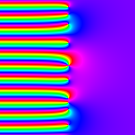
Figure 1. $\arg(\zeta(s))$ for $-9/2\leq\sigma\leq 11/2$, $7000\leq t\leq 7010$.

Thus the argument of $\zeta^{\prime}(\rho)$ plays a significant role in the image, inspiring this MathOverflow question. In this paper we begin the numerical investigation of these by examining $5\cdot 10^{6}$ zeros with $2.63012\cdot 10^{6}\leq\gamma\leq 4.99238\cdot 10^{6}$.

2. Selberg and Hejhal

Starting first with $\zeta(s)$, an unpublished result of Selberg [4, p. 310] implies

Theorem.

Suitably normalized, $\arg(\zeta(1/2+it))$ converges in distribution over fixed ranges to a standard normal variable. More precisely, for $\alpha<\beta$ we have

$$\lim_{T\to\infty}\frac{1}{T}\mu(T\leq t\leq 2T\,|\,\alpha<\frac{\arg(\zeta(1/2+it))}{\sqrt{\log\log(T)/2}}<\beta)=\\ \frac{1}{\sqrt{2\pi}}\int_{\alpha}^{\beta}\exp(-x^{2}/2)\,dx,$$

where $\mu$ is Lebesgue measure.

The argument is the imaginary part of $\log(\zeta(1/2+it))$, computed by continuous variation along a vertical line from, say, $\sigma=4$ to $4+it$ and then along a horizontal line to $1/2+it$. Selberg’s result actually covers the real part of the complex logarithm, $\log|\zeta(1/2+it)|$ as well.

Returning to $\zeta^{\prime}$, for the real part of the logarithm we have the following generalization of Selberg’s result, due to Hejhal [1]:

Theorem.

Assuming the Riemann Hypothesis and a technical condition on the spacing of zeros which is a weak consequence of the Montgomery Pair Correlation Conjecture, then $\log|\zeta^{\prime}(1/2+it)|$, suitably normalized, converges in distribution over fixed ranges to a standard normal variable. More precisely, for $\alpha<\beta$ we have

$$\lim_{N\to\infty}\left|\frac{1}{N}\left\{n:N\leq n\leq 2N,\alpha<\frac{\log\left|\frac{2\pi\zeta^{\prime}(1/2+i\gamma_{n})}{\log(\gamma_{n}/2\pi)}\right|}{\sqrt{\log\log(N)/2}}<\beta\right\}\right|\\ =\frac{1}{\sqrt{2\pi}}\int_{\alpha}^{\beta}\exp(-x^{2}/2)\,dx$$

Here’s my attempt to make an exposition of Hejhal’s exposition [1, p. 346] of the basic idea behind the proof. First some notation: With

$$\chi(s)=\pi^{s-1/2}\frac{\Gamma((1-s)/2)}{\Gamma(s/2)},$$

define $\phi(s)$ by

$$\chi(s)^{-1/2}=\exp(i\phi(s)),$$

so $\phi$ is real on the critical line. Let $M$ be a large constant, $t$ an auxiliary random variable with $T\leq t\leq 2T$, and $W_{t}$ the ’window’

$$W_{t}=[t-M/\log T,t+M/\log T].$$

Let $A(t)=t/2\pi\log\left(t/2\pi\right)-t/2\pi$. Let $x=A(u)$, and $\theta(u)=\phi(1/2+iu)$. Let $P_{t}(x)$ be the polynomial approximation

$$P_{t}(x)=\Pi_{\gamma\in W_{t}}(x-A(\gamma)),$$

and define $\Omega_{t}(u)$ to be the correction to the approximation so that

$$\zeta(1/2+iu)=\exp(\Omega_{t}(u)-i\theta(u))P_{t}(x).$$

Computing logarithmic derivative (in $u$, being careful with the chain rule) we see

$$i\frac{\zeta^{\prime}(1/2+iu)}{\zeta(1/2+iu)}=\Omega_{t}^{\prime}(u)-i\theta^{\prime}(u)+\frac{P_{t}^{\prime}(x)}{P_{t}(x)}\cdot A^{\prime}(u)$$

Rearranging gives

$$i\frac{\zeta^{\prime}(1/2+iu)}{A^{\prime}(u)}=\zeta(1/2+iu)\cdot\left(\frac{\Omega_{t}^{\prime}(u)}{A^{\prime}(u)}-i\frac{\theta^{\prime}(u)}{A^{\prime}(u)}+\frac{P_{t}^{\prime}(x)}{P_{t}(x)}\right).$$

Hejhal makes an estimate (see below) of the term in parenthesis on the right to argue that

$$\frac{\log\left|\zeta(1/2+iu)\right|}{\sqrt{\log\log T}}\quad\text{ and }\quad\frac{\log\left|\zeta^{\prime}(1/2+iu)/A^{\prime}(u)\right|}{\sqrt{\log\log T}}$$

are (in effect) the same random variable, and so Selberg’s theorem applies.

For this estimate, Hejhal claims he and Bombieri showed previously that the total variation of $\Omega_{t}(u)$ on $W_{t}$ is $O_{M}(1)$ for ’most’ $t$. This means

$$\int_{W_{t}}\left|\Omega^{\prime}_{t}(u)\right|du=O_{M}(1)$$

for ’most’ $t$, and so on ’most’ windows $W_{t}$, $\left|\Omega^{\prime}_{t}(u)\right|=O_{M}(\log T)$.

The above was the hard part; $\theta^{\prime}(u)/A^{\prime}(u)$ is elementary. And $P_{t}^{\prime}(x)/P_{t}(x)=\sum_{\gamma\in W_{t}}1/(x-A(\gamma)),$ with average spacing between $A(\gamma)$ being 1 and the number of terms in the sum $O_{M}(1)$. Hejhal argues heuristically that

$$\log\left|\frac{\Omega_{t}^{\prime}(u)}{A^{\prime}(u)}-i\frac{\theta^{\prime}(u)}{A^{\prime}(u)}+\frac{P_{t}^{\prime}(x)}{P_{t}(x)}\right|=O_{M}(1)$$

except for a subset of small measure. This completes Hejhal’s estimate.

Could this heuristic be extended to the imaginary part of
$\log\zeta^{\prime}(1/2+iu)$, defined (again) by continuous variation up the vertical line from $4$ to $4+iu$ and along the horizontal line from $4+iu$ to $1/2+iu$? The challenge is that the estimates above depend on being inside a window of radius $M/\log T$. We will see below that the variation along the vertical line is quite regular, so that presents no problem. Along the horizontal line, between the real part $4$ and the real part $1/2+M/\log T$, the zeros of $\zeta^{\prime}$ should be infrequent and so the argument of $\zeta^{\prime}$ should be changing slowly for ‘most’values of $u$.

3. Algorithm

The first $10^{7}$ zeros of $\zeta(s)$ are implemented constants in Mathematica, which can also, of course, easily compute derivatives numerically. Evaluating the argument via continuous variation requires a little more effort. For a zero $\rho=1/2+i\gamma$, the variation along the line from $4$ to $4+i\gamma$ is easy. In this range

$$\zeta^{\prime}(4+iy)=-\log(2)2^{-4-iy}-\sum_{n=3}^{\infty}\log(n)n^{-4-iy}.$$

The first term has $|\log(2)2^{-4-iy}|=0.0433217$, while the tail is smaller, bounded by $0.025590$, and thus via Rouché theorem $\zeta^{\prime}(4+iy)$ winds around the origin as many times as does $-\log(2)2^{-4-iy}$.

Along the horizontal line $s=x+i\gamma$, $1/2<x\leq 4$, we only need to estimate $\zeta^{\prime}(s)$ very roughly, to determine when the argument increases by a multiple of $2\pi$. Since we compute at many equally spaced points along the line, directly computing each derivative in Mathematica is wasteful and slow. Instead we make a table of values of $\zeta(s)$ at the equally spaced points, and use a variant of Richardson Interpolation [3, 5.7] of the derivative:

$$(-\zeta(s-3\Delta x)+9\zeta(s-2\Delta x)-45\zeta(s-\Delta x)+\\ 45\zeta(s+\Delta x)-9\zeta(s+2\Delta x)+\zeta(s+3\Delta x))/60\Delta x=\\ \zeta^{\prime}(s)+O(\Delta x^{6}).$$

(In fact the next term of the $\Delta x$ series expansion of the left side is$\zeta^{(7)}(s)\Delta x^{6}/140$.). The derivative $\zeta^{\prime}(1/2+i\gamma)$ is computed with the built-in Mathematica implemetation.

$k$	$\Delta$
$8546951$	$0.00232317$
$5042996$	$0.00296997$
$9857600$	$0.00302828$
$9675304$	$0.00333645$
$7279824$	$0.00337943$
$7498518$	$0.00387655$
$7060975$	$0.00494052$

Table 1. Small gaps between zeros $\rho_{k}$ of $\zeta(s)$, $5\cdot 10^{6}\leq k\leq 10^{7}$

The step size $\Delta x$ needs to give a sufficiently accurate result even when the horizontal line passes close to a zero of $\zeta^{\prime}(s)$. Recalling that the zeros of $\zeta^{\prime}$ in $\text{Re}(s)>1/2$ tend to be interspersed between the zeros of $\zeta(s)$ on the critical line, we looked for small gaps between successive zeros $\rho_{k}$, $\rho_{k+1}$ for $5\cdot 10^{6}\leq k\leq 10^{7}$. With just seven exceptions (see Table 1), the gaps are all greater than $0.005$. Based on this we choose for speed a step size $\Delta x$ of $0.0025$, accepting that a very small number of phases may be computed incorrectly.

4. Data

Hiary and Odlyzko [2] have investigated Hejhal’s theorem numerically, for data sets at much larger heights than we consider, and find the convergence rather slow. They also observe a surplus of large values and a deficit of small values. Since we have the data available, for completeness we include in Figure 2 a histogram of values, for $5\cdot 10^{6}\leq k\leq 10^{7}$, of

$$\frac{\log|2\pi\zeta^{\prime}(\rho_{k})/\log(\gamma_{k}/2\pi)|}{\sqrt{\log\log(5\cdot 10^{6})}}.$$

Figure 3 is the numerical investigation of the argument, the main goal of the paper. For $5\cdot 10^{6}\leq k\leq 10^{7}$, the histogram displays

$$\frac{\arg\zeta^{\prime}(\rho_{k})+\pi-\gamma_{k}\log 2}{\sqrt{\log\log(5\cdot 10^{6})}}.$$

Mathematica computes the mean to be $-0.00043882$ and the standard deviation to be $2.47623$. For what it is worth, the third through sixth moments were computed to be $0.00463054$, $76.8629$, $0.344781$, and $1333.96$ respectively.

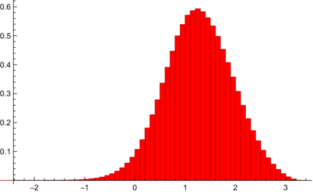
Figure 2. $\log|\zeta^{\prime}(\rho)|$.

Figure 4 shows both the real and imaginary parts of $\log\zeta^{\prime}(\rho_{k})$. Observe that the apparent surplus of examples with the imaginary part near $\pm\pi$ seems to correlate to the real part being positive and relatively large.

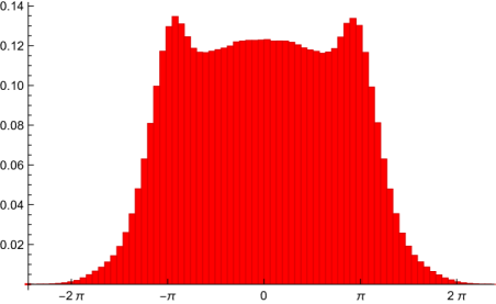
Figure 3. $\arg(\zeta^{\prime}(\rho))$.

5. Summary

Given the poor fit to a (mean $0$) Gaussian for the data in Figure 2, perhaps not much can be conjectured from the data in Figure 3, beyond that there is a distribution for the argument computed by continuous variation. In other words, the naive conjecture that the data are uniform in $(-\pi,\pi]$ appears to be incorrect. We hope this paper inspires others with access to more computing power to investigate further.

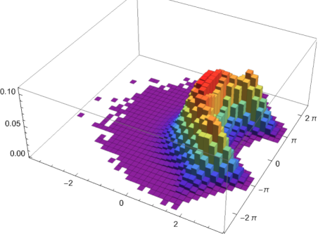
Figure 4. $\log(\zeta^{\prime}(\rho))$.

References

- [1] D.A. Hejhal, On the distribution of , in Number Theory, Trace Formulas, and Discrete Groups, K.E. Aubert, E. Bombieri, D.M. Goldfeld, eds., Proc. 1987 Selberg Symposium, Academic Press, 1989, pp. 343-370.
- [2] G. Hiary and A. Odlyzko, Numerical study of the derivative of the Riemann zeta function at zeros, Commentarii Mathematici Universitatis Sancti Pauli, 60 no. 1-2, (2011) pp. 47-60.
- [3] W. Press et al., Numerical Recipes in C: The Art of Scientific Computing. Cambridge University Press.
- [4] E. Titchmarsh, The Theory of the Riemann Zeta Function, Oxford University Press, 2nd ed., New York, 1986.
- [5] E. Wegert, Visual Complex Functions: An Introduction with Phase Portraits, Birkhäuser, 2012.