Approximating the (Continuous) Fréchet Distance

We describe the first strongly subquadratic time algorithm with subexponential approximation ratio for approximately computing the Fréchet distance between two polygonal chains. Specifically, let $P$ and $Q$ be two polygonal chains with $n$ vertices in $d$-dimensional Euclidean space, and let $\alpha\in[\sqrt{n},n]$. Our algorithm deterministically finds an $O(\alpha)$-approximate Fréchet correspondence in time $O((n^{3}/\alpha^{2})\log n)$. In particular, we get an $O(n)$-approximation in near-linear $O(n\log n)$ time, a vast improvement over the previously best know result, a linear time $2^{O(n)}$-approximation. As part of our algorithm, we also describe how to turn any approximate decision procedure for the Fréchet distance into an approximate optimization algorithm whose approximation ratio is the same up to arbitrarily small constant factors. The transformation into an approximate optimization algorithm increases the running time of the decision procedure by only an $O(\log n)$ factor.

1 Introduction

The Fréchet distance is a commonly used method of measuring the similarity between a pair of curves. Both its standard (continuous) and discrete variants have seen use in map construction and mapping [5, 16], handwriting recognition [27], and protein alignment [23].

Formally, it is defined as follows: Let $P:[1,m]\to\mathbb{R}^{d}$ and $Q:[1,n]\to\mathbb{R}^{d}$ be two curves in $d$-dimensional Euclidean space. We’ll assume $P$ and $Q$ are represented as polygonal chains, meaning there exist ordered vertex sequences $\langle p_{1},\dots,p_{m}\rangle$ and $\langle q_{1},\dots,q_{n}\rangle$ such that $P(i)=p_{i}$ for all $1\leq i\leq m$, $Q(j)=q_{j}$ for all $1\leq j\leq n$, and both $P$ and $Q$ are linearly parameterized along line segments or edges between these positions. We define a re-parameterization $\sigma:[0,1]\to[1,m]$ of $P$ as any continuous, non-decreasing function such that $\sigma(0)=1$ and $\sigma(1)=m$. We define a re-parameterization $\theta:[0,1]\to[1,n]$ of $Q$ similarly. We define a Fréchet correspondence between $P$ and $Q$ as a pair $(\sigma,\theta)$ of re-parameterizations of $P$ and $Q$ respectively, and we say any pair of reals $(\sigma(r),\theta(r))$ for any $0\leq r\leq 1$ are matched by the correspondence. Let $\mathtt{d}(p,q)$ denote the Euclidean distance between points $p$ and $q$ in $\mathbb{R}^{d}$. The cost of the correspondence is defined as

$$\mu((\sigma,\theta)):=\max_{0\leq r\leq 1}\mathtt{d}(P(\sigma(r)),Q(\theta(r))).$$

Let $\Pi_{\mathsf{FD}}$ denote the set of all Fréchet correspondences between $P$ and $Q$. The (continuous) Fréchet distance of $P$ and $Q$ is defined as

$$\mathsf{FD}(P,Q):=\min_{(\sigma,\theta)\in\Pi_{\mathsf{FD}}}\mu((\sigma,\theta)).$$

The standard intuition given for this definition is to imagine a person and their dog walking along $P$ and $Q$, respectively, without backtracking. The person must keep the dog on a leash, and the goal is to pace their walks as to minimize the length of leash needed to keep them connected. There also exists a variant of the distance called the discrete Fréchet distance where the input consists of two finite point sequences. Here, we replace the person and dog by two frogs. Starting with both frogs on the first point of their sequences, we must iteratively move the first, the second, or both frogs to the next point in their sequences. As before, the goal is to minimize the maximum distance between the frogs.

Throughout this paper, we assume $2\leq m\leq n$. We can easily compute the discrete Fréchet distance in $O(mn)$ time using dynamic programming. The first polynomial time algorithm for computing the continuous case was described by Alt and Godau [6]. They use parametric search [17, 25] and a quadratic time decision procedure (see Section 2) to compute the Fréchet distance in $O(mn\log n)$ time. Almost two decades passed before Agarwal et al. [3] improved the running time for the discrete case to $O(mn\log\log n/\log n)$. Buchin et al. [14] later improved the running time for the continuous case to $O(mn(\log\log n)^{2})$ (these latter two results assume we are working in the word RAM model of computation).

Recently, Gudmundsson et al. [21] described an $O(n\log n)$ time algorithm for computing the continuous distance between chains $P$ and $Q$ assuming all edges have length a sufficiently large constant larger than $\mathsf{FD}(P,Q)$. In short, having long edges allows one to greedily move the person and dog along their respective chains while keeping their leash length optimal.

From this brief history, one may assume substantially faster algorithms are finally forthcoming for general cases of the continuous and discrete Fréchet distance. Unfortunately, more meaningful improvements may not be possible; Bringmann [10] showed that strongly subquadratic ($n^{2-\Omega(1)}$) time algorithms would violate the Strong Exponential Time Hypothesis (SETH) that solving CNF-SAT over $n$ variables requires $2^{(1-o(1))n}$ time [22].

Therefore, we are motivated to look for fast approximation algorithms for these problems. Aronov et al. [8] described a $(1+\varepsilon)$-approximation algorithm for the discrete Fréchet distance. This algorithm runs in subquadratic and often near-linear time if $P$ or $Q$ fall into one of a few different “realistic” families of curves such as ones modeling protein backbones. Driemel et al. [18] describe a $(1+\varepsilon)$-approximation for the continuous Fréchet distance that again runs more quickly if one of the curves belongs to a realistic family than it would otherwise. This latter algorithm was improved for some cases by Bringmann and Künnemann [12]. In the same work mentioned above, Gudmundsson et al. [21] described a $\sqrt{d}$-approximation algorithm that runs in linear time if the input polygonal chains have sufficiently long edges.

Approximation appears more difficult when the input is arbitrary. Bringmann [10] showed there is no strongly subquadratic time $1.001$-approximation for the Fréchet distance, assuming SETH. For arbitrary point sequences, Bringmann and Mulzer [13] described an $O(\alpha)$-approximation algorithm for the discrete distance for any $\alpha\in[1,n/\log n]$ that runs in $O(n\log n+n^{2}/\alpha)$ time. Chan and Rahmati [15] later described an $O(n\log n+n^{2}/\alpha^{2})$ time $O(\alpha)$-approximation algorithm for the discrete distance for any $\alpha\in[1,\sqrt{n/\log n}]$.

For the continuous Fréchet distance over arbitrary polygonal chains, the only strongly subquadratic time algorithm known with bounded approximation ratio runs in linear time but has an exponential worst case approximation ratio of $2^{\Theta(n)}$. This result is described in the same paper of Bringmann and Mulzer [13] mentioned above. We note that there is also a substantial body of work on the (approximate) nearest neighbor problem using Fréchet distance as the metric; see Mirzanezhad [26] for a survey of recent results. These results assume the query curve or the curves being searched are short, so they do not appear directly useful in approximating the Fréchet distance between two curves of arbitrary complexity.

The closely related problems of computing the dynamic time warping and geometric edit distances have a similar history to that of the discrete Fréchet distance. They have straightforward quadratic time dynamic programming algorithms that have been improved by (sub-)polylogarithmic factors for some low dimensional cases [20]; substantial improvements to these algorithms violate SETH or other complexity theoretic assumptions [9, 1, 11, 2]; and there are fast $(1+\varepsilon)$-approximation algorithms specialized for realistic input sequences [4, 28]. And, there exist some approximation results for arbitrary point sequences as well. Kuszmaul [24] described $O((n^{2}/\alpha)\mathop{\mathrm{polylog}}n)$ time $O(\alpha)$-approximation algorithms for dynamic time warping distance over point sequences in well separated tree metrics of exponential spread and geometric edit distance over point sequences in arbitrary metrics. Fox and Li [19] described a randomized $O(n\log^{2}n+(n^{2}/\alpha^{2})\log n)$ time $O(\alpha)$-approximation algorithm for geometric edit distance for points in low dimensional Euclidean space. Even better approximation algorithms exist for the traditional string edit distance where all substitutions have cost exactly $1$; see, for example, Andoni and Nosatzki [7].

Each of the above problems for point sequences admit strongly subquadratic approximation algorithms with polynomial approximation ratios when the input comes from low dimensional Euclidean space. However, such a result remains conspicuously absent for the continuous Fréchet distance over arbitrary polygonal chains. One may naturally assume results for the discrete Fréchet distance extend to the continuous case. However, one advantage of discrete Fréchet distance over the continuous case is that input points can only be matched with other input points. The fact that vertices can match with edge interiors in the continuous case makes it much more difficult to make approximately optimal decisions. In addition, we can no longer depend upon certain data structures for testing equality of subsequences in constant time. These structures are largely responsible for the relatively small running times seen in the algorithms of Chan and Rahmati [15] and Fox and Li [19].

Our results

We describe the first strongly subquadratic time algorithm with subexponential approximation ratio for computing Fréchet correspondences between polygonal chains. Let $P$ and $Q$ be two polygonal chains of $m$ and $n$ vertices, respectively, in $d$-dimensional Euclidean space, and let $\alpha\in[\sqrt{n},n]$. Again, we assume $m\leq n$. Our algorithm deterministically finds a Fréchet correspondence between $P$ and $Q$ of cost $O(\alpha)\cdot\mathsf{FD}(P,Q)$ in time $O((n^{3}/\alpha^{2})\log n)$. In particular, we get an $O(n)$-approximation in near-linear $O(n\log n)$ time, a vast improvement over Bringmann and Mulzer’s [13] linear time $2^{O(n)}$-approximation for continuous Fréchet distance. Our algorithm employs a novel combination of ideas from the original exact algorithm of Alt and Godau [6] for continuous Fréchet distance, the algorithm of Chan and Rahmati [15] for approximating the discrete Fréchet distance, and Gudmundsson et al.’s [21] greedy approach for computing the Fréchet distance between chains with long edges.

Let $\delta>0$. We describe an approximate decision procedure that either determines $\mathsf{FD}(P,Q)>\delta$ or finds a Fréchet correspondence of cost $O(\alpha)\cdot\delta$. The exact decision procedure of Alt and Godau [6] computes a set of reachability intervals in the free space diagram of $P$ and $Q$ with respect to $\delta$ (see Section 2). These intervals represent all points on a single edge of $Q$ that can be matched to a vertex of $P$ (or vice versa) in a Fréchet correspondence of cost at most $\delta$. For our approximate decision procedure, we compute a set of approximate reachability intervals such that the re-parameterizations realizing these intervals have cost $O(\alpha)\cdot\delta$. We cannot afford to compute intervals for all $\Theta(mn)$ vertex-edge pairs, so we instead focus on $O(n^{2}/\alpha^{2})$ vertex-edge pairs as described below that contain the first and last vertices and edges of both chains. The approximate interval we compute for any vertex-edge pair contains the exact interval for that same pair. So if $\mathsf{FD}(P,Q)\leq\delta$, we are guaranteed $(p_{m},q_{n})$ is approximately reachable and our desired Fréchet correspondence exists.

The vertex-edge pairs chosen to hold the approximate reachability intervals follow from ideas of Chan and Rahmati [15]. Similar to them, we place a grid of side length $\alpha\cdot\delta$ so that at most $O(n/\alpha)$ vertices of $P$ and $Q$ lie within distance $3\delta$ of the side of a grid box. We call these $O(n/\alpha)$ vertices bad and the rest good. Also, we call any edge with a bad endpoint bad. Our approximate reachability intervals involve only bad edges and vertices with at least one bad incident edge. To compute these intervals, we describe a method for tracing how a Fréchet correspondence of cost $\delta$ must behave starting from one approximate reachability interval until it reaches some others we wish to compute. Recall, an approximate reachability interval corresponds to pairs of points on $P$ and $Q$ that could be matched together. Either the next edge of $P$ or $Q$ after one of these pairs to leave a box is good and therefore long, or it is bad, and we can afford to compute some new approximate reachability intervals using this edge. We can easily compute correspondences between long edges and arbitrary length edges on the other curve, and we can greedily match the portions of the curves before they leave the box at cost at most $O(\alpha)\cdot\delta$. The traces take only $O(n)$ time each, and we perform at most $O(n^{2}/\alpha^{2})$ traces, so our decision procedure takes $O(n^{3}/\alpha^{2})$ time total.

We would like to use our approximate decision procedure as a black box to compute a Fréchet correspondence of cost $O(\alpha)\cdot\mathsf{FD}(P,Q)$ without knowing $\mathsf{FD}(P,Q)$ in advance. Unfortunately, we are unaware of any known general method to do so. Therefore, we describe how to turn any approximate decision procedure into an algorithm with the same approximation ratio up to arbitrarily small constant factors after an $O(\log n)$ factor increase in running time. In particular, any improvement to our approximate decision procedure would immediately carry over to our overall approximation algorithm. Our method involves binary searching over a set of $O(n)$ values approximating distances between pairs of vertices. If there is a large gap between the Fréchet distance and the nearest of these values, we can simplify both $P$ and $Q$ without losing much accuracy in the Fréchet distance computation while allowing us to use the long edge exact algorithm of Gudmundsson et al. [21].

The rest of our paper is organized as follows. We describe preliminary notions in Section 2. We describe our decision procedure in Section 3 and how to turn it into an approximation algorithm in Section 4. We conclude with some closing thoughts in Section 5.

2 Preliminaries

Let $R:[1,n]\to\mathbb{R}^{d}$ be a polygonal chain in $d$-dimensional Euclidean space. We let $R[r,r^{\prime}]$ denote the restriction of $R$ to $[r,r^{\prime}]$. In other words, the notation refers to the portion of $R$ between points $R(r)$ and $R(r^{\prime})$. We generally use $s$ to refer to members of the domain of a polygonal chain $P$ and $t$ to refer to members of the domain of a polygonal chain $Q$. We use $i$ and $j$, respectively, when these members are integers. Recall, $p_{i}=P(i)$ for all $1\leq i\leq m$ and $q_{j}=Q(j)$ for all $1\leq j\leq n$. We use superscript notation ($s^{a}$) to label particular members of these domains (and not to take the $a$th power of $s$), and we use subscript notation ($s_{k}$) when we are working with an ordered list of these members.

Free space diagram and reachability

Let $P:[1,m]\to\mathbb{R}^{d}$ and $Q:[1,n]\to\mathbb{R}^{d}$ be polygonal chains. Fix some $\delta>0$. Alt and Godau [6] introduced the free space diagram to decide if $\mathsf{FD}(P,Q)\leq\delta$. It consists of a set of pairs $F=\left\{(s,t)\in[1,m]\times[1,n]\right\}$. Each $(s,t)\in F$ represents the pair of points $P(s)$ and $Q(t)$. Point $(s,t)\in F$ is free if $\mathtt{d}(P(s),Q(t))\leq\delta$. The free space $\mathcal{D}_{\leq\delta}(P,Q)$ consists of all free points between $P$ and $Q$ for a given $\delta$. Formally, it is given by the set $\mathcal{D}_{\leq\delta}(P,Q):=\{(s,t)\in[1,m]\times[1,n]:\mathtt{d}(P(s),Q(t))\leq\delta\}$. We say that a point $(s^{\prime},t^{\prime})\in F$ is reachable if there exists an $s$ and $t$-monotone path from $(1,1)$ to $(s^{\prime},t^{\prime})$ through $\mathcal{D}_{\leq\delta}(P,Q)$.

The standard procedure for determining if $\mathsf{FD}(P,Q)\leq\delta$ divides $F$ into cells $C_{i,j}:=[i-1,i]\times[j-1,j]$ for all $i\in\left\langle 2,\dots,m\right\rangle$ and $j\in\left\langle 2,\dots,n\right\rangle$. The intersection of a cell $C_{i,j}$ with the free space is convex [6]. The intersection of an edge of the free space diagram cell $C_{i,j}$ with the free space forms a free space interval. The subset of reachable points within a free space interval form what is called an (exact) reachability interval. We say a Fréchet correspondence $(\sigma,\theta)$ between $P$ and $Q$ uses or passes through a reachability interval if there exists some point $(\sigma(r),\theta(r))$ within that interval.

Given the bottom and left reachability intervals of a free space diagram cell, we can compute the top and right reachability intervals of the same cell in $O(1)$ time [6]. The exact decision procedure loops through the cells in increasing order of $i$ and $j$, computing reachability intervals one-by-one. Let $\alpha\in[\sqrt{n},n]$. We cannot afford to compute all $\Theta(mn)$ reachability intervals, so instead we compute $O(n^{2}/\alpha^{2})$ ($\alpha$)-approximate reachability intervals. The approximate reachability intervals are subsets of the free space intervals such that for any point $(s,t)$ on an approximate reachability interval, there exists a Fréchet correspondence between $P[1,s]$ and $Q[1,t]$ of cost $O(\alpha)\cdot\delta$. We express exact or approximate reachability intervals by the subset of $F$ they contain; for example, given $j-1\leq t^{a}\leq t^{b}\leq j$, we will use $\left\{i\right\}\times[t^{a},t^{b}]$ to refer to an interval on the right side of cell $C_{i,j}$.

Grids, good points, bad points, and dangerous points

Chan and Rahmati [15] utilize a $d$-dimensional grid to create the useful notion of good and bad vertices for their discrete Fréchet distance approximation algorithm. We adopt their use of a $d$-dimensional grid. Unlike Chan and Rahmati, however, we are no longer working with sequences of discrete points but instead polygonal chains. We must therefore define new constructs of good and bad that work better for our problem’s input.

Let $P:[1,m]\to\mathbb{R}^{d}$ and $Q:[1,n]\to\mathbb{R}^{d}$ be two polygonal chains. Fix $\delta>0$ and $\alpha\in[\sqrt{n},n]$. Let $G$ be a $d$-dimensional grid consisting of boxes of side length $\alpha\cdot\delta$. (We do not use the term cell here to avoid confusion with the free space diagram.) We say a vertex of $P$ or $Q$ is good if it is more than distance $3\delta$ from any edge of $G$. If a vertex is not good, then we call it bad. For simplicity, we also designate $p_{1}$, $q_{1}$, $p_{m}$, and $q_{n}$ as bad, regardless of their position within boxes of $G$.

We also extend the constructs of good and bad to the edges of $P$ and $Q$. We say an edge on either chain is good if both its endpoints are good vertices. Otherwise, the edge is bad. Lastly, we say that a vertex is dangerous (but not necessarily good or bad) if at least one of its incident edges is bad. Chan and Rahmati [15, Lemma 1] demonstrate how to compute a grid $G$ with $O(n/\alpha)$ bad vertices in $O(n)$ time. Because each bad vertex has up to two incident edges, there are also $O(n/\alpha)$ bad edges. Each bad edge is incident to two vertices, so there are $O(n/\alpha)$ dangerous vertices as well. Our approximate decision procedure will compute approximate reachability intervals only between dangerous vertices and bad edges. Therefore, there will be at most $O(n^{2}/\alpha^{2})$ such intervals.

Curve simplification

Let $R:[1,n]\to\mathbb{R}^{d}$ be a polygonal chain with vertices $\left\langle r_{1},\dots,r_{n}\right\rangle$. Our approximation algorithm relies on a method for simplifying chains so their edges are not too short. We slightly modify of a procedure of Driemel et al. [18]. Let $\nu>0$ be a parameter. We mark $r_{1}$ and set it as the current vertex. We then repeat the following procedure until we no longer have a designated current vertex. We scan $R$ from the current vertex until reaching the first vertex $r_{i}$ of distance at least $\nu$ from the current vertex. We mark $r_{i}$, set it as the current vertex, and perform the next iteration of the loop. The $\nu$-simplification of $R$, denoted $\hat{R}$, is the polygonal chain consisting of exactly the marked vertices in order. Note that unlike Driemel et al. [18], we do not require the final vertex of $R$ to be marked. We can easily verify that all edges of $\hat{R}$ have length at least $\nu$. Also, $\mathsf{FD}(R,\hat{R})\leq\nu$ [18, Lemma 2.3].

3 Approximate Decision Procedure

In this section, we present our $O(\alpha)$-approximate decision procedure. Let $P:[1,m]\to\mathbb{R}^{d}$ and $Q:[1,n]\to\mathbb{R}^{d}$ be two polygonal chains in $d$-dimensional Euclidean space as defined before, and let $\alpha\in[\sqrt{n},n]$. Let $\delta>0$. We begin by computing the grid $G$ along with $O(n/\alpha)$ bad edges and points as defined in Section 2. We then explicitly compute and record a set of $O(n^{2}/\alpha^{2})$ approximate reachability intervals between dangerous vertices and bad edges. To compute these intervals, we occasionally perform a linear time greedy search for a good correspondence. We describe this greedy search procedure in Section 3.1 before giving the remaining details of the decision procedure in Section 3.2.

3.1 Greedy mapping subroutines

We describe a pair of subroutines for greedily computing Fréchet correspondences along lengths of $P$ and $Q$. The first of these procedures $\textsc{GreedyMappingP}(i,t)$ takes as its input an integer $i\in\left\langle 1,\dots,m\right\rangle$ such that $p_{i}$ is a good vertex of $P$ along with a real value $t\in[1,n]$ such that $\mathtt{d}(p_{i},Q(t))\leq\delta$. Informally, the procedure does the following: Suppose there exists a Fréchet correspondence $(\sigma,\theta)$ between $P$ and $Q$ of cost at most $\delta$ that maps $p_{i}$ ‘close to’ $Q(t)$. Procedure $\textsc{GreedyMappingP}(i,t)$ essentially follows $P$ and $Q$ from box to box, discovering groups of points that must be matched by $(\sigma,\theta)$. When there is too much ambiguity in what must be matched to continue searching greedily, it outputs a set of approximate reachability intervals, including one used by $(\sigma,\theta)$. While we can infer which boxes pairs of matched points belong to, it may still be unclear exactly which pairs appear in $(\sigma,\theta)$. Also, the procedure may output intervals despite $(\sigma,\theta)$ not existing in the first place! Therefore, we can only guarantee the intervals can be reached using a correspondence of cost at most $O(\alpha)\cdot\delta$. We define another procedure $\textsc{GreedyMappingQ}(j,s)$ similarly, exchanging the roles of $P$ and $Q$. As they are rather technical, the precise definitions of these procedures are best expressed in the following lemmas.

Lemma 3.1

Let $i\in\left\langle 1,\dots,m\right\rangle$ and $t\in[1,n]$ such that $p_{i}$ is good and $\mathtt{d}(p_{i},Q(t))\leq\delta$. Procedure $\textsc{GreedyMappingP}(i,t)$ outputs zero or more approximate reachability intervals between a bad edge of $P$ or $Q$ and a dangerous vertex of $Q$ or $P$, respectively. For each pair $(s^{\prime},t^{\prime})\in[i,m]\times[t,n]$ in an approximate reachability interval computed by the procedure, there exists a Fréchet correspondence of cost $O(\alpha)\cdot\delta$ between $P[i,s^{\prime}]$ and $Q[t,t^{\prime}]$. Procedure $\textsc{GreedyMappingQ}(j,s)$ has the same properties with the roles of $P$ and $Q$ exchanged.

Lemma 3.2

Let $i\in\left\langle 1,\dots,m\right\rangle$ and $t\in[1,n]$ such that $p_{i}$ is good and $\mathtt{d}(p_{i},Q(t))\leq\delta$. Suppose there exists a Fréchet correspondence $(\sigma,\theta)$ between $P$ and $Q$ of cost at most $\delta$ that matches $i$ with some $t^{*}\geq t$ such that every point of $Q[t,t^{*}]$ is at most distance $3\delta$ from $p_{i}$. Then, $(\sigma,\theta)$ passes through at least one approximate reachability interval output by procedure $\textsc{GreedyMappingP}(i,t)$. Procedure $\textsc{GreedyMappingQ}(j,s)$ has the same properties with the roles of $P$ and $Q$ exchanged.

We now provide details on the implementation of $\textsc{GreedyMappingP}(i,t)$ along with intuition for the steps it uses. Procedure $\textsc{GreedyMappingQ}(j,s)$ has an analogous description, with the roles of $P$ and $Q$ exchanged.

To begin, observe $p_{i}$ and $Q(t)$ lie in the same box $B$ of grid $G$, because $p_{i}$ is good and $\mathtt{d}(p_{i},Q(t))\leq\delta$. We first follow $P$ and $Q$ to see where they leave $B$: Let $s^{e}=m$ if $P$ never leaves $B$ after $p_{i}$. Otherwise, let $s^{e}$ be the minimum value in $(i,m]$ such that $P(s^{e})$ lies on the boundary of $B$ (the ‘$e$’ stands for exit). Define $t^{e}$ similarly for $Q$. See Figure 3.1.

If either curve ends before leaving $B$, then the rest of the other curve needs to stay near $B$ if a correspondence like in Lemma 3.2 exists. Therefore, if $s^{e}=m$ (resp. $t^{e}=n$), we check if all points of $Q[t,n]$ (resp. $P[i,m]$) lie in or within distance $\delta$ of $B$. If so, we output the trivial approximate reachability interval of $\left\{(m,n)\right\}$ and terminate the procedure. Otherwise, we output zero approximate reachability intervals.

From here on, we assume $s^{e}\neq m$ and $t^{e}\neq n$. Let $i^{e}\in\left\langle 1,\dots,m\right\rangle$ such that $i^{e}-1\leq s^{e}\leq i^{e}$, and define $j^{e}$ similarly. We begin by considering cases where a curve leaves box $B$ along a good edge. Here, a correspondence as described in Lemma 3.2 must match a portion of the other curve to the good edge. Fortunately, we can guess approximately where that portion of the other curve begins and ends. Afterward, the other endpoint of the good edge serves as a suitable parameter for a recursive call to one of our greedy mapping procedures.

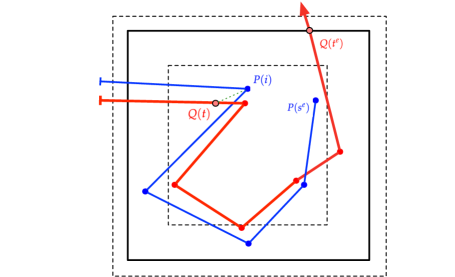
Figure 3.1: Basic setup for $\textsc{GreedyMappingP}(i,t)$

Specifically, suppose edge $P[i^{e}-1,i^{e}]$ is good. In this case, let $t^{f}$ be the minimum value in $(t,n]$ such that $\mathtt{d}(p_{i^{e}},Q(t^{f}))\leq\delta$, and let $t^{c}$ be the maximum value in $[t,t^{f})$ such that $\mathtt{d}(p_{i^{e}-1},Q(t^{c}))\leq\delta$ (the ‘$f$’ stands for far, and the ‘$c$’ stands for close). See Figure 3.2. We check if every point of $Q[t,t^{c}]$ lies in or within distance $\delta$ of $B$ and if $\mathsf{FD}(P[i^{e}-1,i^{e}],Q[t^{c},t^{f}])\leq\delta$. If so, we run $\textsc{GreedyMappingP}(i^{e},t^{f})$ and use its output. Otherwise, we output zero approximate reachability intervals.

Now suppose the previous case does not hold but edge $Q[j^{e}-1,j^{e}]$ is good. Here, we perform similar steps to those described in the previous case, exchanging the roles of $P$ and $Q$. Specifically, we let $s^{f}$ be the minimum value in $(i,m]$ such that $\mathtt{d}(q_{j^{e}},P(s^{f}))\leq\delta$, and let $s^{c}$ be the maximum value in $[i,s^{f})$ such that $\mathtt{d}(q_{j^{e}-1},Q(s^{c}))\leq\delta$. We check if every point of $P[i,s^{c}]$ lies in or within distance $\delta$ of $B$ and if $\mathsf{FD}(P[s^{c},s^{f}],Q[j^{e}-1,j^{e}])\leq\delta$. If so, we run $\textsc{GreedyMappingQ}(j^{e},s^{f})$ and use its output. Otherwise, we output zero approximate reachability intervals.

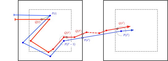
Figure 3.2: $\textsc{GreedyMappingP}(i,t)$: The case where $P[i^{e}-1,i^{e}]$ is good

From here on, we assume neither curve leaves box $B$ through a good edge. Suppose there is a correspondence $(\sigma,\theta)$ as described in Lemma 3.2. Further suppose the reparameterized walks along $P$ and $Q$ leave box $B$ along $P$ before $Q$. In this case, we can show that $P(s^{e})$ is matched with a point on a bad edge of $Q$. Accordingly, we iterate over the bad edges of $Q$ that appear before $Q$ leaves box $B$, computing sufficiently large approximate reachability intervals along the top and right sides of free space diagram cells for $P[i^{e}-1,i^{e}]$ and those bad edges of $Q$. Both of the edges for each of these cells are bad, so the intervals we compute are between bad edges and dangerous vertices.

Specifically, let $t\leq t_{1}<t_{2}<\dots<t_{\ell}\leq t^{e}$ be the list of first positions along their respective edges of $Q$ such that $\mathtt{d}(P(s^{e}),Q(t_{k}))\leq\delta$ for each $k\in\left\langle 1,\dots,\ell\right\rangle$. See Figure 3.3, left. Observe that each edge containing a point $t_{k}$ must be bad, because $Q$ does not leave $B$ along a good edge, and no good edge with two endpoints in $B$ lies within distance $\delta$ of $P(s^{e})$. For each $k\in\left\langle 1,\dots,\ell\right\rangle$, we do the following: Let $j_{k}\in\left\langle 1,\dots,n\right\rangle$ such that $j_{k}-1\leq t_{k}\leq j_{k}$. Let $t^{a}_{k}$ be the minimum value in $[t_{k},j_{k}]$ such that $\mathtt{d}(p_{i^{e}},Q(t^{a}_{k}))\leq\delta$ and let $t^{b}_{k}$ be the maximum value in $[t_{k},j_{k}]$ such that $\mathtt{d}(p_{i^{e}},Q(t^{b}_{k}))\leq\delta$. If $t^{a}_{k}$ and $t^{b}_{k}$ are well-defined, then we designate the interval $\left\{i^{e}\right\}\times[t^{a}_{k},t^{b}_{k}]$ as approximately reachable. (If we have already designated a subset of $\left\{i^{e}\right\}\times[j_{k}-1,j_{k}]$ as approximately reachable earlier in the decision procedure, then we extend the approximately reachable area by taking the union with the old interval. Every interval of $\left\{i^{e}\right\}\times[j_{k}-1,j_{k}]$ we compute will end at $(i^{e},t^{b}_{k})$, so the union is also an interval.) Similarly, let $s^{a}_{k}$ be the minimum value in $[s^{e},i^{e}]$ such that $\mathtt{d}(P(s^{a}_{k}),q_{j_{k}})\leq\delta$ and let $s^{b}_{k}$ be the maximum value in $[s^{e},i^{e}]$ such that $\mathtt{d}(P(s^{b}_{k}),q_{j_{k}})\leq\delta$. If $s^{a}_{k}$ and $s^{b}_{k}$ are well-defined, then we designate the interval $[s^{a}_{k},s^{b}_{k}]\times\left\{j_{k}\right\}$ as approximately reachable. See Figure 3.3, right.

It is also possible that a good correspondence has the walk along $Q$ leave box $B$ first. So, in addition to the above set of approximate reachability intervals, we also create some based on points of $P$ between $p_{i}$ and $P(s^{e})$ that pass close to $Q(t^{e})$. Let $s\leq s_{1}<s_{2}<\dots<s_{\ell}\leq s^{e}$ be the exhaustive list of first positions along their respective edges of $P$ such that $\mathtt{d}(P(s_{k}),Q(t^{e}))\leq\delta$ for each $k\in\left\langle 1,\dots,\ell\right\rangle$. For each $k\in\left\langle 1,\dots,\ell\right\rangle$, we do the following: Let $i_{k}\in\left\langle 1,\dots,n\right\rangle$ such that $i_{k}-1\leq s_{k}\leq i_{k}$. Let $s^{a}_{k}$ be the minimum value in $[s_{k},i_{k}]$ such that $\mathtt{d}(P(s^{a}_{k}),q_{j^{e}})\leq\delta$, and let $s^{b}_{k}$ be the maximum value in $[s_{k},i_{k}]$ such that $\mathtt{d}(P(s^{b}_{k}),q_{j^{e}})\leq\delta$. If $s^{a}_{k}$ and $s^{b}_{k}$ are well-defined, then we designate the interval $[s^{a}_{k},s^{b}_{k}]\times\left\{j^{e}\right\}$ as approximately reachable. Similarly, let $t^{a}_{k}$ be the minimum value in $[t^{e},j^{e}]$ such that $\mathtt{d}(p_{j_{k}},Q(t^{a}_{k}))\leq\delta$, and let $t^{b}_{k}$ be the maximum value in $[t^{e},j^{e}]$ such that $\mathtt{d}(p_{j_{k}},Q(t^{b}_{k}))\leq\delta$. If $t^{a}_{k}$ and $t^{b}_{k}$ are well-defined, then we designate the interval $\left\{i_{k}\right\}\times[t^{a}_{k},t^{b}_{k}]$ as approximately reachable.

We have concluded our description of $\textsc{GreedyMappingP}(i,t)$ and are ready to prove Lemmas 3.1 and 3.2.

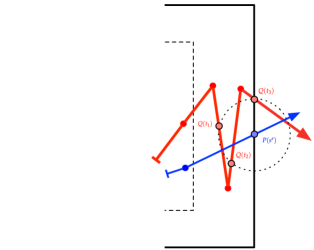
Figure 3.3: Left: Definition of $\left\langle t_{1},\dots,t_{\ell}\right\rangle$. Right: Designating approximate reachability intervals near a pair $(s^{e},t_{k})$. The clipped ellipse coincides with the free points inside cell $C_{i^{e},j_{k}}$.

• We use the same notation as given in the description of$\textsc{GreedyMappingP}(i,t)$. We first argue that we only output reachability intervals between bad edges and dangerous vertices. If we only output the trivial interval $\left\{(m,n)\right\}$ then the statement is trivially true. Otherwise, suppose we create an interval while working with $P(s^{e})$ and some nearby point $Q(t_{k})$. We are not performing a recursive call to GreedyMappingP in this case, so $P[i^{e}-1,i^{e}]$ is bad, and $p_{i^{e}}$ is dangerous. Similarly, we are not performing a recursive call to GreedyMappingQ, so $Q[j^{k}-1,j^{k}]$ is not a good edge with endpoint $q_{j^{k}}$ outside of box $B$. Point $Q(t_{k})$ is within distance $\delta$ of the boundary of $B$, so $Q[j_{k}-1,j_{k}]$ cannot be a good edge with both endpoints in $B$, either. We conclude $Q[j_{k}-1,j_{k}]$ is bad as well, and $q_{j_{k}}$ is dangerous. A similar argument holds if we create an interval while working with $Q(t^{e})$ and some nearby point of $P$.

  We now argue that for any pair of points $(s^{\prime},t^{\prime})$ on one of the approximate reachability intervals output by the procedure, there exists a correspondence of cost $O(\alpha)\cdot\delta$ between $P[i,s^{\prime}]$ and $Q[t,t^{\prime}]$. First, suppose $\textsc{GreedyMappingP}(i,t)$ creates one or more approximate reachability intervals without performing a recursive call. Suppose $s^{e}=m$ or $t^{e}=n$, implying $(s^{\prime},t^{\prime})=(m,n)$. All points of $P[i,m]$ and $Q[t,n]$ lie in or within distance $\delta$ of $B$, so they are all distance at most $\sqrt{d}(\alpha+1)\cdot\delta$ from each other and any Fréchet correspondence between $P[i,s^{\prime}]$ and $Q[t,t^{\prime}]$ has cost $O(\alpha)\cdot\delta$.

  Now suppose otherwise, but $(s^{\prime},t^{\prime})$ lies on an interval created while working with $P(s^{e})$ and some nearby point $Q(t_{k})$. All points of $P[i,s^{e}]$ and $Q[t,t_{k}]$ lie in $B$, so they are all distance at most $\sqrt{d}\alpha\cdot\delta$ from each other and any Fréchet correspondence between $P[i,s^{e}]$ and $Q[t,t_{k}]$ has cost $O(\alpha)\cdot\delta$. The set of pairs $(x,y)\in P[i^{e}-1,i^{e}]\times Q[j_{k}-1,j_{k}]$ such that $\mathtt{d}(P(x),Q(y))\leq\delta$ includes $(s^{e},t_{k})$ and $(s^{\prime},t^{\prime})$, and the set is convex [6], so we can extend our correspondence to include another between $P[s^{e},s^{\prime}]$ and $Q[t_{k},t^{\prime}]$ of cost at most $\delta$. A similar argument covers the case where $(s^{\prime},t^{\prime})$ lies on an interval created while working with $Q(t^{e})$ and a nearby point of $P$.

  Finally, suppose $\textsc{GreedyMappingP}(i,t)$ recursively calls $\textsc{GreedyMappingP}(i^{e},t^{f})$. Every point of $P[i,i^{e}-1]$ and $Q[t,t^{c}]$ lies in or within distance $\delta$ of $B$, so every correspondence between $P[i,i^{e}-1]$ and $Q[t,t^{c}]$ has cost at most $O(\alpha)\cdot\delta$. Also, we have $\mathsf{FD}(P[i^{e}-1,i^{e}],Q[t^{c},t^{f}])\leq\delta$. We can combine these correspondences with the one inductively guaranteed by the call to $\textsc{GreedyMappingP}(i^{e},t^{f})$ to get our desired correspondence between $P[i,s^{\prime}]$ and $Q[t,t^{\prime}]$. Again, a similar argument covers the case where we do a recursive call $\textsc{GreedyMappingQ}(j^{e},s^{f})$.

  The proof for $\textsc{GreedyMappingQ}(j,s)$ is the same, but with the roles of $P$ and $Q$ exchanged.

• We use the same notation as given in the description of$\textsc{GreedyMappingP}(i,t)$. By assumption and the fact that $p_{i}$ is good, every point of $Q[t,t^{*}]$ lies within $B$. Let $r^{se}=\sigma^{-1}(s^{e})$ and $r^{te}=\theta^{-1}(t^{e})$.

  Suppose $\textsc{GreedyMappingP}(i,t)$ does not do a recursive call. If we output the trivial interval $\left\{(m,n)\right\}$, then the lemma is trivially true. Suppose we do not output the trivial interval and $r^{se}\leq r^{te}$. Point $Q(\theta(r^{se}))$ lies on an edge $Q[j_{k}-1,j_{k}]$ with one of the points $Q(t_{k})$ where $\mathtt{d}(P(s^{e}),Q(t_{k}))\leq\delta$. By definition of $t_{k}$, we have $t_{k}\leq\theta(r^{se})$. Recall, the free space is convex within each individiaul cell of the free space diagram [6]. Therefore, the set of $s^{e}\leq s^{\prime}\leq i^{e}$ such that $\mathsf{FD}(P[s^{e},s^{\prime}],Q[\theta(r^{se}),j_{k}])\leq\delta$ is precisely the approximate reachability interval $[s^{a}_{k},s^{b}_{k}]\times\left\{j_{k}\right\}$ we computed. Similarly, the set of $\theta(r^{se})\leq t^{\prime}\leq j_{k}$ such that $\mathsf{FD}(P[s^{e},i^{e}],Q[\theta(r^{se}),t^{\prime}])\leq\delta$ is actually a suffix of the approximate reachability interval $\left\{i^{e}\right\}\times[t^{a}_{k},t^{b}_{k}]$ we computed. A similar argument applies if $r^{te}<r^{se}$.

  Finally, suppose $\textsc{GreedyMappingP}(i,t)$ recursively calls $\textsc{GreedyMappingP}(i^{e},t^{f})$. Let $t^{f*}$ be matched with $i^{e}$ and $t^{c*}$ be matched with $i^{e}-1$ by $(\sigma,\theta)$. Because $p_{i^{e}-1}$ and $p_{i^{e}}$ are both good, $\mathtt{d}(p_{i^{e}-1},Q(t^{c*}))\leq\delta$, and $\mathtt{d}(p_{i^{e}},Q(t^{f}))\leq\delta$, points $Q(t^{c*})$ and $Q(t^{f})$ lie within the same boxes as $p_{i^{e}-1}$ and $p_{i^{e}}$, respectively. These boxes are distinct, so we may conclude $t^{c*}\leq t^{f}$. Further, we chose $t^{c}\geq t^{c*}$ and $t^{f}\leq t^{f*}$, and we may infer $Q(t^{c})$ and $Q(t^{f*})$ also lie in the same boxes as $p_{i^{e}-1}$ and $p_{i^{e}}$, respectively. We conclude $t^{c*}\leq t^{c}<t^{f}\leq t^{f*}$.

  Consider the following correspondence between $P[i^{e}-1,i^{e}]$ and $Q[t^{c},t^{f}]$: Let $s^{c}\geq i^{e}-1$ and $s^{f}\leq i^{e}$ be matched to $t^{c}$ and $t^{f}$, respectively, by $(\sigma,\theta)$. We match every point of $P[i^{e}-1,s^{c}]$ to $Q(t^{c})$, match $P[s^{c},s^{f}]$ to $Q[t^{c},t^{f}]$ exactly as done by $(\sigma,\theta)$, and match every point of $P[s^{f},i^{e}]$ to $Q(t^{f})$. See Figure 3.4. We have $\mathtt{d}(p_{i^{e}-1},Q(t^{c}))\leq\delta$ and $\mathtt{d}(P(s^{c}),Q(t^{c}))\leq\delta$, so the entire line segment $P[i^{e}-1,s^{c}]$ lies within distance $\delta$ of $Q(t^{c})$. Similarly, the line segment $P[s^{f},i^{e}]$ lies within distance $\delta$ of $Q(t^{f})$. Our correspondence has cost at most $\delta$.

  

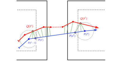
  Figure 3.4: A correspondence of cost $\delta$ between $P[i^{e}-1,i^{e}]$ and $Q[t^{c},t^{f}]$. A subset of matched points are represented by thin green line segments.

Now, consider any point $Q(t^{\prime})$ with $t^{c*}\leq t^{\prime}\leq t^{c}$ and let $s^{\prime}$ be matched to $t^{\prime}$ by $(\sigma,\theta)$. We have $\mathtt{d}(P(s^{\prime}),Q(t^{\prime}))\leq\delta$. We argued that line segment $P[i^{e}-1,s^{c}]$ is within distance $\delta$ of $Q(t^{c})$, implying $\mathtt{d}(P(s^{\prime}),Q(t^{c}))\leq\delta$. Finally, $\mathtt{d}(p_{i^{e}-1},Q(t^{c}))\leq\delta$. By triangle inequality, $\mathtt{d}(p_{i^{e}-1},Q(t^{\prime}))\leq 3\delta$, implying $Q(t^{\prime})$ lies in $B$. As explained above, every point of $Q[t,t^{*}]$ lies in $B$. Also, every point of $Q[t^{*},t^{c*}]$ lies within distance $\delta$ of a point in $P[i,i^{e}-1]$ and therefore lies in or within distance $\delta$ of $B$. And, we just showed every point of $Q[t^{c*},t^{c}]$ lies in $B$. Our algorithm will succeed at all its distance checks and recursively call $\textsc{GreedyMappingP}(i^{e},t^{f})$. Finally, a similar triangle inequality argument implies every point of $Q[t^{f},t^{*f}]$ is at most distance $3\delta$ from $p_{i^{e}}$. We are inductively guaranteed that $(\sigma,\theta)$ passes through an approximate reachability interval output during the recursive call. Similar arguments apply if $\textsc{GreedyMappingP}(i,t)$ does a recursive call $\textsc{GreedyMappingQ}(j^{e},s^{f})$.

The proof for $\textsc{GreedyMappingQ}(j,s)$ is the same as that given above, but with the roles of $P$ and $Q$ exchanged.

3.2 Remaining decision procedure details

We now fill in the remaining details of our approximate decision procedure. Recall, we have computed a grid $G$ with boxes of side length $\alpha\cdot\delta$ such that there are $O(n/\alpha)$ bad vertices of $P$ and $Q$. Also recall, $p_{1}$, $p_{m}$, $q_{1}$, and $q_{n}$ are designated as bad regardless of their position in $G$’s boxes. As described below, our decision procedure, iteratively in lexicographic order, checks each cell of the free space diagram for which we may have computed an approximate reachablity interval on its left or bottom side. We then extend the known approximately reachable space from each non-empty interval in one of two ways. Depending on whether relevant edges are good or bad, we either perform a call to the appropriate greedy mapping subroutine to seek out new intervals that are approximately reachable but potentially far away in the free space diagram, or we directly compute approximate reachability intervals on the right or top sides of the cell using the constant time method of Alt and Godau [6].

Specifically, we first check if $\mathtt{d}(p_{1},q_{1})\leq\delta$. If not, our procedure reports failure. Otherwise, let $t^{b}$ and $s^{b}$ be the maximum values in $[1,2]$ such that $\mathtt{d}(p_{1},Q(t^{b}))\leq\delta$ and $\mathtt{d}(P(s^{b}),q_{1})\leq\delta$, respectively. We designate intervals $\left\{1\right\}\times[1,t^{b}]$ and $[1,s^{b}]\times\left\{1\right\}$ as (approximately) reachable. Now, for each $i\in\left\langle 2,\dots,m\right\rangle$ such that $p_{i-1}$ is dangerous, for each $j\in\left\langle 2,\dots,n\right\rangle$ such that $q_{j-1}$ is dangerous, we do the following.

Suppose we have designated an interval $\left\{i-1\right\}\times[t^{a},t^{b}]$ as approximately reachable where $j-1\leq t^{a}\leq t^{b}\leq j$. Suppose edge $P[i-1,i]$ is good. Then, we run the procedure $\textsc{GreedyMappingP}(i-1,t^{a})$. If edge $P[i-1,i]$ is bad, we compute new approximate reachability intervals more directly as follows. First, let $t^{a^{\prime}}$ be the minimum value in $[t^{a},j]$ such that $\mathtt{d}(p_{i},Q(t^{a^{\prime}}))\leq\delta$, and let $t^{b^{\prime}}$ be the maximum value in $[t^{a},j]$ such that $\mathtt{d}(p_{i},Q(t^{b^{\prime}}))\leq\delta$. We designate interval $\left\{i\right\}\times[t^{a^{\prime}},t^{b^{\prime}}]$ as approximately reachable (again, we may end up extending a previously computed approximately reachability interval on $\left\{i\right\}\times[j-1,j]$). Similarly, let $s^{a^{\prime}}$ be the minimum value in $[i-1,i]$ such that $\mathtt{d}(P(s^{a^{\prime}}),q_{j})\leq\delta$, and let $s^{b^{\prime}}$ be the maximum value in $[i-1,i]$ such that $\mathtt{d}(P(s^{a^{\prime}}),q_{j})\leq\delta$. We designate interval $[s^{a^{\prime}},s^{b^{\prime}}]\times\left\{j\right\}$ as approximately reachable. We are done working with interval $\left\{i-1\right\}\times[t^{a},t^{b}]$.

Now, suppose we have designated interval $[s^{a},s^{b}]\times\left\{j-1\right\}$ as approximately reachable where $i-1\leq s^{a}\leq s^{b}\leq i$. Suppose edge $Q[j-1,j]$ is good. If so, we run the procedure $\textsc{GreedyMappingQ}(j-1,s^{a})$. If edge $Q[j-1,j]$ is bad, we compute new approximate reachability intervals more directly as follows. First, let $t^{a^{\prime}}$ be the minimum value in $[j-1,j]$ such that $\mathtt{d}(p_{i},Q(t^{a^{\prime}}))\leq\delta$, and let $t^{b^{\prime}}$ be the maximum value in $[j-1,j]$ such that $\mathtt{d}(p_{i},Q(t^{b^{\prime}}))\leq\delta$. We designate interval $\left\{i\right\}\times[t^{a^{\prime}},t^{b^{\prime}}]$ as approximately reachable. Similarly, let $s^{a^{\prime}}$ be the minimum value in $[s^{a},i]$ such that $\mathtt{d}(P(s^{a^{\prime}}),q_{j})\leq\delta$, and let $s^{b^{\prime}}$ be the maximum value in $[s^{b},i]$ such that $\mathtt{d}(P(s^{a^{\prime}}),q_{j})\leq\delta$. We designate interval $[s^{a^{\prime}},s^{b^{\prime}}]\times\left\{j\right\}$ as approximately reachable. We are done working with interval $[s^{a},s^{b}]\times\left\{j-1\right\}$.

Once we have completed the iterations, we do one final step. We check if $(m,n)$ lies on an approximate reachability interval. If so, we report there is a Fréchet correspondence between $P$ and $Q$ of cost $O(\alpha)\cdot\delta$. Otherwise, we report failure.

The following lemmas establish the correctness and running time for our decision procedure.

Lemma 3.3

The approximate decision procedure creates approximate reachability intervals only between bad edges of $P$ or $Q$ and dangerous vertices of $Q$ or $P$, respectively.

• Vertices $p_{1}$ and $q_{1}$ are bad, so the intervals we compute before beginning the for loops are between bad edges and dangerous vertices. Now, consider working with some approximate reachability interval $\left\{i-1\right\}\times[t^{a},t^{b}]$ with $j-1\leq t^{a}\leq t^{b}\leq j$. Inductively, we may assume $Q[j-1,j]$ is bad, implying $q_{j}$ is dangerous. If $P[i-1,i]$ is good, then Lemma 3.1 guarantees we only create approximate reachability intervals between bad edges and dangerous vertices. Otherwise, $p_{i}$ is dangerous, and both approximate reachability intervals we directly create are for bad edge/dangerous vertex pairs. A similar argument applies when working with some interval $[s^{a},s^{b}]\times\left\{j-1\right\}$.

Lemma 3.4

The approximate decision procedure is correct if it reports $\mathsf{FD}(P,Q)\leq O(\alpha)\cdot\delta$.

• Let $(s^{\prime},t^{\prime})$ be any member of an approximate reachability interval created by the procedure. We will show there exists a Fréchet correspondence between $P[1,s^{\prime}]$ and $Q[1,t^{\prime}]$ of cost $O(\alpha)\cdot\delta$. Setting $(s^{\prime},t^{\prime})=(m,n)$ then proves the lemma. First, if $(s^{\prime},t^{\prime})$ lies on either interval created before the for loops begin, there is a trivial correspondence between $P[1,s^{\prime}]$ and $Q[1,t^{\prime}]$ of cost at most $\delta$ that only uses one point of either $P$ or $Q$. Now, consider working with some approximate reachability interval $\left\{i-1\right\}\times[t^{a},t^{b}]$ with $j-1\leq t^{a}\leq t^{b}\leq j$. Inductively, we may assume there is a correspondence of cost $O(\alpha)\cdot\delta$ between $P[1,i-1]$ and $Q[1,t^{a}]$.

  Suppose $P[i-1,i]$ is good, and we call $\textsc{GreedyMappingP}(i-1,t^{a})$. By Lemma 3.1, we can extend our inductively guaranteed correspondence to one of cost $O(\alpha)\cdot\delta$ ending at any point $(s^{\prime},t^{\prime})$ in any approximate reachability interval output by $\textsc{GreedyMappingP}(i-1,t^{a})$. Now, suppose instead that $P[i-1,i]$ is bad. As in the proof of Lemma 3.1 or the original exact algorithm of Alt and Godau [6], there is a Fréchet correspondence of cost at most $\delta$ between $P[i-1,s^{\prime}]$ and $Q[t^{a},t^{\prime}]$ for any $(s^{\prime},t^{\prime})$ on the approximate reachability intervals we directly compute. Again, we can extend the inductively guaranteed correspondence to end at any such $(s^{\prime},t^{\prime})$. A similar argument applies when working with some interval $[s^{a},s^{b}],\times\left\{j-1\right\}$.

Lemma 3.5

Suppose there exists a Fréchet correspondence $(\sigma,\theta)$ between $P$ and $Q$ of cost at most $\delta$. The approximate decision procedure will report $\mathsf{FD}(P,Q)\leq O(\alpha)\cdot\delta$.

• Suppose $(\sigma,\theta)$ matches a pair $(i-1,t^{*})$ on some approximate reachability interval $\left\{i-1\right\}\times[t^{a},t^{b}]$. Suppose $P[i-1,i]$ is good. Every point of $Q[t^{a},t^{*}]$ lies within distance $\delta$ of $p_{i-1}$. Lemma 3.2 guarantees $\textsc{GreedyMappingP}(i-1,t^{a})$ will output at least one approximate reachability interval which includes a matched pair of $(\sigma,\theta)$. We can easily verify that the interval must involve a later vertex of $P$ than $p_{i-1}$.

  Now, suppose instead that $P[i-1,i]$ is bad. The set of $i-1\leq s^{\prime}\leq i$ such that $\mathsf{FD}(P[i-1,s^{\prime}],Q[t^{*},j])\leq\delta$ is precisely the approximate reachability interval $[s^{a^{\prime}},s^{b^{\prime}}]\times\left\{j\right\}$ we computed. Similarly, the set of $t^{*}\leq t^{\prime}\leq j$ such that $\mathsf{FD}(P[i-1,i],Q[t^{*},t^{\prime}])\leq\delta$ is actually a suffix of the approximate reachability interval $\left\{i\right\}\times[t^{a^{\prime}},t^{b^{\prime}}]$ we computed.

  Either way, we have $(\sigma,\theta)$ using an interval for a later vertex of $P$ or $Q$. If the interval contains $(m,n)$, the decision procedure will report there exists a cheap correspondence. Otherwise, we may assume it will report one inductively. Similar arguments apply if $(\sigma,\theta)$ includes a point on some approximate reachability interval $[s^{a},s^{b}]\times\left\{j-1\right\}$.

  Finally, we observe that $(\sigma,\theta)$ does include a point on at least one approximate reachability interval, because our procedure begins by computing two intervals that include $(1,1)$.

Lemma 3.6

Procedures $\textsc{GreedyMappingP}(i,t)$ and $\textsc{GreedyMappingQ}(j,s)$ can be implemented to run in $O(n)$ time.

• We use the notation given in the description of GreedyMappingP. Let $m^{\prime}=m-i+1$, and let $n^{\prime}$ be the number of vertices remaining in $Q$ after $Q(t)$. If $s^{e}=m$ or $t^{e}=n$, then we spend $O(m^{\prime}+n^{\prime})$ time checking if a suffix of $P$ and $Q$ lies in or near box $B$. From here, assume neither $s^{e}=m$ nor $t^{e}=n$.

  Suppose edge $P[i^{e}-1,i^{e}]$ is good. Let $m^{\prime\prime}=i^{e}-i\geq 1$, and let $n^{\prime\prime}$ be the number of vertices in $Q[t,t^{f}]$. We need to scan $P$ and $Q$ to find $i^{e}$, $t^{c}$, and $t^{f}$. We also need to check if every point of $Q[t,t^{c}]$ lies in or close to $B$. Doing these steps takes $O(m^{\prime\prime}+n^{\prime\prime})$ time. We need to check if $\mathsf{FD}(P[i^{e}-1,i^{e}],Q[t^{c},t^{f}])\leq\delta$. The portion of $P$ in this check consists of a single line segment, so it can be done in $O(n^{\prime\prime})$ time. Finally, we do a recursive call to $\textsc{GreedyMappingP}(i^{e},t^{f})$ that inductively takes $O(n^{\prime}+m^{\prime}-n^{\prime\prime}-m^{\prime\prime})$ time. In total, we spend $O(n^{\prime}+m^{\prime})$ time. A similar argument holds if $P[i^{e}-1,i^{e}]$ is bad but $Q[j^{e}-1,j^{e}]$ is good.

  Finally, suppose both edges are bad. We spend $O(n^{\prime}+m^{\prime})$ time total searching for $s^{e}$ and $t^{e}$, finding points from the other curve that lie close to $s^{e}$ and $t^{e}$, and computing approximate reachability intervals for each of these pairs of points.

Lemma 3.7

The approximate decision procedure can be implemented to run in $O(n^{3}/\alpha^{2})$ time.

• Finding the grid $G$ with the set of $O(n/\alpha)$ bad vertices takes $O(n)$ time [15, Lemma 1]. There are at most twice as many bad edges as bad vertices, and at most twice as many dangerous vertices as bad edges, so there are $O(n/\alpha)$ dangerous vertices. Therefore, the decision procedure iterates over $O(n^{2}/\alpha^{2})$ values of $i$ and $j$. For each pair, we do at most two $O(n)$ time calls to GreedyMappingP or GreedyMappingQ, or we compute up to four approximate reachability intervals directly in constant time each.

Our decision procedure is easily extended to actually output a correspondence of cost $O(\alpha)\cdot\delta$ instead of merely determining if one exists by concatenating the smaller correspondences we discover directly during the iterations or during runs of GreedyMappingP and GreedyMappingQ as we compute approximate reachability intervals. We are now able to state the main result of this section.

Lemma 3.8

Let $P$ and $Q$ be two polygonal chains in $\mathbb{R}^{d}$ of at most $n$ vertices each, let $\alpha\in[\sqrt{n},n]$, and let $\delta\geq 0$ be a parameter. We can compute a Fréchet correspondence between $P$ and $Q$ of cost at most $O(\alpha)\cdot\delta$ or verify that $\mathsf{FD}(P,Q)>\delta$ in $O(n^{3}/\alpha^{2})$ time.

4 The Approximation Algorithm

We now describe how to turn our approximate decision procedure into an approximation algorithm whose approximation ratio is arbitrarily close to that of the decision procedure. We emphasize that our techniques use the decision procedure as a black box subroutine, so any improvement to the running time of our approximate decision procedure will imply the same improvement to our approximation algorithm. In short, we use our approximate decision procedure to binary search over a set of $O(n)$ distances approximating the distances between vertices of $P$ and $Q$. If the Fréchet distance lies in a large enough gap between a pair of these approximate distances, then we can simplify both polygonal chains so that their edge lengths become large compared to their Fréchet distance. We then run an exact Fréchet distance algorithm of Gudmundsson et al. [21] designed for this case.

Let $P:[1,m]\to\mathbb{R}^{d}$ and $Q:[1,n]\to\mathbb{R}^{d}$ be two polygonal chains in $d$-dimensional Euclidean space, and suppose we have an approximate decision procedure for the Fréchet distance between two polygonal chains with approximation ratio $\alpha$. We assume $\alpha$ is at most a polynomial function of $n$ (although it may be constant). Let $T(n,\alpha)$ denote the worst-case running time of the procedure on two polygonal chains of at most $n$ vertices each. We assume $T(n,\alpha)=\Omega(n)$. Finally, consider any $0<\varepsilon\leq 1$. We describe how to compute an $O((1+\varepsilon)\alpha)$-approximation of $\mathsf{FD}(P,Q)$ in $O(T(n,\alpha)\log(n/\varepsilon))$ time.

We begin by performing a binary search over a set $Z$ of $O(n)$ values close to all of the distances between pairs of vertices in $P$ and $Q$. Let $V$ denote the set of vertex points in $P$ and $Q$. Our set $Z$ is such that for any pair of distinct points $o_{1},o_{2}\in V$, there exist $x,x^{\prime}\in Z$ such that $x\leq\mathtt{d}(o_{1},o_{2})\leq x^{\prime}\leq 2x$. Such a set can be computed in $O(n\log n)$ time [18, Lemma 3.9]. To perform the binary search, we simply search “down” if the approximate decision procedure finds an $\alpha$-approximate correspondence, and we search “up” if it does not. Let $a$ and $b$ be the largest value of $Z$ for which the procedure fails and the smallest value for which it succeeds, respectively. If $a$ does not exist, then we return the correspondence of cost $\alpha\cdot b$ found for $b$. We are guaranteed $b$ exists, because the maximum distance between $P$ and $Q$ is achieved at a pair of vertices. From here on, we assume $a$ exists.

We check if the approximate decision procedure finds a correspondence when given parameter $\delta:=12a/\varepsilon$. If so, let $Z^{a}$ denote the sequence of distances $\left\langle(1+\varepsilon)^{0}\cdot a,(1+\varepsilon)^{1}\cdot a,\dots,(1+\varepsilon)^{\left\lceil 12/\varepsilon\right\rceil}\cdot a\right\rangle$. We binary search over $Z^{a}$ and return the cheapest correspondence found.

Suppose no correspondence is found for $12a/\varepsilon$. We check if the approximate decision procedure finds a correspondence when given parameter $\delta:=b/(2(1+\varepsilon/2)(1+\sqrt{d})\alpha)$. If not, let $Z^{b}$ denote the sequence of distances $\left\langle b/(1+\varepsilon)^{0},b/(1+\varepsilon)^{1},\dots,b/(1+\varepsilon)^{\left\lceil 2(1+\varepsilon/2)(1+\sqrt{d})\alpha\right\rceil}\right\rangle$. We binary search over $Z^{b}$ and return the cheapest correspondence found.

Finally, suppose no correspondence is found for $12a/\varepsilon$ but one is found for $b/(2(1+\varepsilon/2)(1+\sqrt{d})\alpha)$. We perform a $3a$-simplification of $P$ and $Q$, yielding the polygonal chains $\hat{P}$ and $\hat{Q}$ with at most $n$ vertices each. Gudmundsson et al. [21] describe an $O(n\log n)$ time algorithm that computes the Fréchet distance of two polygonal chains exactly if all of their edges have length at least $(1+\sqrt{d})$ times their Fréchet distance. Their algorithm will succeed in finding an optimal Fréchet correspondence between $\hat{P}$ and $\hat{Q}$. This correspondence can be modified to create one for $P$ and $Q$ of cost at most $(1+\varepsilon)\alpha\cdot\mathsf{FD}(P,Q)$ (see Driemel et al. [18, Lemmas 2.3 and 3.5]).

Lemma 4.1

The approximation algorithm finds a correspondence between $P$ and $Q$ of cost at most $(1+\varepsilon)\alpha\cdot\mathsf{FD}(P,Q)$.

• Suppose value $a$ as defined in the procedure does not exist. We find a correspondence of cost at most $\alpha\cdot b\leq\alpha\cdot\mathtt{d}(p_{1},q_{1})\leq\alpha\cdot\mathsf{FD}(P,Q)$. We assume from here on that $a$ exists.

  Suppose a binary search over $Z^{a}$ or $Z^{b}$ is performed. There exist values $a^{\prime}$ and $b^{\prime}=(1+\varepsilon)a^{\prime}$ such that the approximate decision procedure fails with $a^{\prime}$ but succeeds at finding a correspondence of cost at most $\alpha\cdot b^{\prime}$. We have $\alpha\cdot b^{\prime}=(1+\varepsilon)\alpha\cdot a^{\prime}<(1+\varepsilon)\alpha\cdot\mathsf{FD}(P,Q)$.

  Finally, suppose we perform binary searches over neither $Z^{a}$ nor $Z^{b}$. In this case, we observe $12a/\varepsilon<\mathsf{FD}(P,Q)\leq b/(2(1+\varepsilon/2)(1+\sqrt{d}))$. Every distance between a pair of vertices in $P$ or $Q$ is either at most $2a<(\varepsilon/6)\mathsf{FD}(P,Q)$ or at least $b/2\geq(1+\sqrt{d})(1+\varepsilon/2)\mathsf{FD}(P,Q)$. We observe $\mathsf{FD}(\hat{P},\hat{Q})\leq\mathsf{FD}(P,Q)+6a<(1+\varepsilon/2)\mathsf{FD}(P,Q)$ [18, Lemma 2.3]. Polygonal chains $\hat{P}$ and $\hat{Q}$ have no edges of length at most $2a$, implying all edges have length at least $(1+\sqrt{d})(1+\varepsilon/2)\mathsf{FD}(P,Q)>(1+\sqrt{d})\mathsf{FD}(\hat{P},\hat{Q})$. The conditions for the algorithm of Gudmundsson et al. [21] are met, and as explained earlier, their algorithm will lead to the desired correspondence between $P$ and $Q$.

Lemma 4.2

The approximation algorithm can be implemented to run in $O(T(n,\alpha)\log(n/\varepsilon))$ time.

• We spend $O(n\log n)$ time computing $Z$. We do $O(\log n)$ calls to the approximate decision procedure binary searching over $Z$. Sequences $Z^{a}$ and $Z^{b}$ contain $O(\log_{1+\varepsilon}(1/\varepsilon))=O((1/\varepsilon)\log(1/\varepsilon))$ and $O(\log_{1+\varepsilon}\alpha)=O((1/\varepsilon)\log n)$ values, respectively. Therefore, binary searching over $Z^{a}$ or $Z^{b}$ requires $O(\log((1/\varepsilon)\log(n/\varepsilon)))=O(\log(n/\varepsilon))$ calls to the approximate decision procedure. The case where we have to simplify the polygonal chains and run the algorithm of Gudmundsson et al. [21] requires only $O(n\log n)$ additional time. The lemma follows.

We may now state the main result of this section.

Theorem 4.3

Suppose we have an $\alpha$-approximate decision procedure for Fréchet distance that runs in time $T(n,\alpha)$ on two polygonal chains in $\mathbb{R}^{d}$ of at most $n$ vertices each. Let $0<\varepsilon\leq 1$. Given two such chains $P$ and $Q$, we can find a Fréchet correspondence between $P$ and $Q$ of cost at most $(1+\varepsilon)\alpha\cdot\mathsf{FD}(P,Q)$ in $O(T(n,\alpha)\log(n/\varepsilon))$ time.

Combining Theorem 4.3 with Lemma 3.8 while setting $\varepsilon:=1$ gives us our main result.

Corollary 4.4

Let $P$ and $Q$ be two polygonal chains in $\mathbb{R}^{d}$ of at most $n$ vertices each, and let $\alpha\in[\sqrt{n},n]$. We can compute a Fréchet correspondence between $P$ and $Q$ of cost at most $O(\alpha)\cdot\mathsf{FD}(P,Q)$ in $O((n^{3}/\alpha^{2})\log n)$ time.

5 Conclusion

We described the first strongly subquadratic time approximation algorithm for the continuous Fréchet distance that has a subexponential approximation guarantee. Specifically, it computes an $O(\alpha)$-approximate Fréchet correspondence in $O((n^{3}/\alpha^{2})\log n)$ time for any $\alpha\in[\sqrt{n},n]$. We admit that our result is not likely the best running time one can achieve and that it serves more as a first major step toward stronger results. In particular, we are at a major disadvantage compared to the $O(n\log n+n^{2}/\alpha^{2})$ time algorithm of Chan and Rahmati [15] for discrete Fréchet distance in that they rely on a constant time method for testing subsequences of points for equality and we know of no analogous procedure for quickly testing (near) equality of subcurves. However, it may not be the case that our own running time analysis is even tight; perhaps a more involved analysis applied to a slight modification of our decision procedure could lead to a better running time. We leave open further improvements such as the one described above.

Acknowledgements

The authors would like to thank Karl Bringmann and Marvin Künnemann for some helpful discussions concerning turning an approximate decision procedure into a proper approximation algorithm.

References

- [1] Amir Abboud, Arturs Backurs, and Virginia Vassilevska Williams. Tight hardness results for LCS and other sequence similarity measures. In Proc. 56th Ann. IEEE Symp. Found. Comp. Sci., pages 59–78, 2015.
- [2] Amir Abboud, Thomas Dueholm Hansen, Virginia Vassilevska Williams, and Ryan Williams. Simulating branching programs with edit distance and friends: Or: a polylog shaved is a lower bound made. In Proc. 48th Ann. ACM Sympos. Theory of Comput., pages 375–388, 2016.
- [3] Pankaj K. Agarwal, Rinat Ben Avraham, Haim Kaplan, and Micha Sharir. Computing the discrete Fréchet distance in subquadratic time. SIAM J. Comput., 43(2):429–449, 2014.
- [4] Pankaj K. Agarwal, Kyle Fox, Jiangwei Pan, and Rex Ying. Approximating dynamic time warping and edit distance for a pair of point sequences. In Proc. 32nd Int. Conf. Comput. Geom., pages 6:1–6:16, 2016.
- [5] Mahmuda Ahmed, Sophia Karagiorgou, Dieter Pfoser, and Carola Wenk. Map Construction Algorithms. Springer, 2015.
- [6] Helmut Alt and Michael Godau. Computing the Fréchet distance between two polygonal curves. Int. J. Comput. Geom. Appl., 5:75–91, 1995.
- [7] Alexandr Andoni and Negev Shekel Nosatzki. Edit distance in near-linear time: it’s a constant factor. In Proc. 61st Ann. IEEE Symp. Found. Comput. Sci., 2020.
- [8] Boris Aronov, Sariel Har-Peled, Christian Knauer, Yusu Wang, and Carola Wenk. Fréchet distance for curves, revisited. In Proc. 14th Ann. Euro. Sympos. Algo., pages 52–63, 2006.
- [9] Arturs Backurs and Piotr Indyk. Edit distance cannot be computed in strongly subquadratic time (unless SETH is false). SIAM J. Comput., 47(3):1087–1097, 2018.
- [10] Karl Bringmann. Why walking the dog takes time: Fréchet distance has no strongly subquadratic algorithms unless SETH fails. In Proc. 55th. Ann. IEEE Symp. Found. Comp. Sci., pages 661–670, 2014.
- [11] Karl Bringmann and Marvin Künnemann. Quadratic conditional lower bounds for string problems and dynamic time warping. In Proc. 56th Ann. IEEE Symp. Found. Comp. Sci., pages 79–97, 2015.
- [12] Karl Bringmann and Marvin Künnemann. Improved approximation for Fréchet distance on -packed curves matching conditional lower bounds. Int. J. Comput. Geom. Appl., 27(1-2):85–120, 2017.
- [13] Karl Bringmann and Wolfgang Mulzer. Approximability of the discrete Fréchet distance. J. Comput. Geom., 7(2):46–76, 2016.
- [14] Kevin Buchin, Maike Buchin, Wouter Meulemans, and Wolfgang Mulzer. Four Soviets walk the dog: Improved bounds for computing the Fréchet distance. Discrete Comput. Geom., 58(1):180–216, 2017.
- [15] Timothy M. Chan and Zahed Rahmati. An improved approximation algorithm for the discrete Fréchet distance. Inf. Process. Lett., 138:72–74, 2018.
- [16] Daniel Chen, Anne Driemel, Leonidas J. Guibas, Andy Nguyen, and Carola Wenk. Approximate map matching with respect to the Fréchet distance. In Proc. 13th Meeting on Algorithm Engineering and Experiments, pages 75–83, 2011.
- [17] Richard Cole. Slowing down sorting networks to obtain faster sorting algorithms. J. ACM, 34(1):200–208, 1987.
- [18] Anne Driemel, Sariel Har-Peled, and Carola Wenk. Approximating the Fréchet distance for realistic curves in near linear time. Discrete Comput. Geom., 48(1):94–127, 2012.
- [19] Kyle Fox and Xinyi Li. Approximating the geometric edit distance. In Proc. 30th Int. Symp. Algo. Comput., pages 26:1–26:16, 2019.
- [20] Omer Gold and Micha Sharir. Dynamic time warping and geometric edit distance: Breaking the quadratic barrier. ACM Trans. Algorithms, 14(4):50:1–50:17, 2018.
- [21] Joachim Gudmundsson, Majid Mirzanezhad, Ali Mohades, and Carola Wenk. Fast Fréchet distance between curves with long edges. Int. J. Comput. Geom. Appl., 29(2):161–187, 2019.
- [22] Russell Impagliazzo and Ramamohan Paturi. On the complexity of k-SAT. J. Comp. Sys. Sci., 62(2):367–375, 2001.
- [23] Minghui Jiang, Ying Xu, and Binhai Zhu. Protein structure-structure alignment with discrete Fréchet distance. J. Bioinformatics and Computational Biology, 6(1):51–64, 2008.
- [24] William Kuszmaul. Dynamic time warping in strongly subquadratic time: Algorithms for the low-distance regime and approximate evaluation. In Proc. 46th Intern. Colloqu. Automata, Languages, Programming, pages 80:1–80:15, 2019.
- [25] Nimrod Megiddo. Applying parallel computation algorithms in the design of serial algorithms. J. Assoc. Comput. Mach., 30(4):852–865, 1983.
- [26] Majid Mirzanezhad. On the approximate nearest neighbor queries among curves under the Fréchet distance. CoRR, abs/2004.08444, 2020. URL: https://arxiv.org/abs/2004.08444, arXiv:2004.08444.
- [27] E. Sriraghavendra, K. Karthik, and Chiranjib Bhattacharyya. Fréchet distance based approach for searching online handwritten documents. In Proc. 9th Intern. Conf. Document Analysis and Recognition, pages 461–465, 2007.
- [28] Rex Ying, Jiangwei Pan, Kyle Fox, and Pankaj K. Agarwal. A simple efficient approximation algorithm for dynamic time warping. In Proc. 24th ACM SIGSPATIAL Int. Conf. Adv. Geo. Inf. Sys., 2016.