Faster Uncertainty Quantification for Inverse Problems with Conditional Normalizing Flows

Abstract

In inverse problems, we often have access to data consisting of paired samples $(x,y)\sim p_{X,Y}(x,y)$ where $y$ are partial observations of a physical system, and $x$ represents the unknowns of the problem. Under these circumstances, we can employ supervised training to learn a solution $x$ and its uncertainty from the observations $y$. We refer to this problem as the “supervised” case. However, the data $y\sim p_{Y}(y)$ collected at one point could be distributed differently than observations $y^{\prime}\sim p_{Y}^{\prime}(y^{\prime})$, relevant for a current set of problems. In the context of Bayesian inference, we propose a two-step scheme, which makes use of normalizing flows and joint data to train a conditional generator $q_{\theta}(x|y)$ to approximate the target posterior density $p_{X|Y}(x|y)$. Additionally, this preliminary phase provides a density function $q_{\theta}(x|y)$, which can be recast as a prior for the “unsupervised” problem, e.g. when only the observations $y^{\prime}\sim p_{Y}^{\prime}(y^{\prime})$, a likelihood model $y^{\prime}|x$, and a prior on $x^{\prime}$ are known. We then train another invertible generator with output density $q^{\prime}_{\phi}(x|y^{\prime})$ specifically for $y^{\prime}$, allowing us to sample from the posterior $p_{X|Y}^{\prime}(x|y^{\prime})$. We present some synthetic results that demonstrate considerable training speedup when reusing the pretrained network $q_{\theta}(x|y^{\prime})$ as a warm start or preconditioning for approximating $p_{X|Y}^{\prime}(x|y^{\prime})$, instead of learning from scratch. This training modality can be interpreted as an instance of transfer learning. This result is particularly relevant for large-scale inverse problems that employ expensive numerical simulations.

1 Introduction

Deep learning techniques have recently benefited inverse problems where the unknowns defining the state of a physical system and related observations are jointly available as solution-data paired samples [see, for example, 1]. Throughout the text, we will refer to this problem as the “supervised” case. Supervised learning can be readily applied by training a deep network to map the observations to the respective solution, often leading to competitive alternatives to solvers that are purely based on a physical model for the data likelihood (e.g. PDEs) and prior (handcrafted) regularization. Unfortunately, for many inverse problems such as seismic or optoacoustic imaging, data is scarce due to acquisition costs, processing is computationally complex because of numerical simulation, and the physical parameters of interest cannot be directly verified. Furthermore, as in the seismic case, the vast diversity of geological scenarios is bound to impact the generalization capacity of the learned model. For this type of problem, supervised methods have still limited scope with respect to more traditional “unsupervised” approaches, e.g. where observations pertaining to a single unknown are available, a data model and prior are postulated, and generalization errors do not affect the results. Note that recent work has found an application for deep networks even in the unsupervised setting as a reparameterization of the unknowns and an implicit regularizing prior [deep prior, 2, 3, 4, 5, 6, 7], by constraining the solution to its range. Unless the network has been adequately pretrained, however, the deep prior approach does not offer computational advantages.

In practice, as it is often the case in seismic or medical imaging, some legacy joint data might be available for supervised learning, while we might be interested in solving a problem related to some new observations, which are expected to come from a moderate perturbation of the legacy (marginal) distribution. In this work, we are interested in combining the supervised and unsupervised settings, as described above, by exploiting the supervised result as a way to accelerate the computation of the solution for the unsupervised problem. Clearly, this is all the more relevant when we wish to quantify the uncertainty in the proposed solution.

This paper is based on exploiting conditional normalizing flows [8, 9] as a way to encapsulate the joint distribution of observations/solution for an inverse problem, and the posterior distribution of the solutions given data. Recent advancements have made available invertible flows that allow analytic computation of such posterior densities. Therefore, we propose a general two-step scheme which consists of: (i) learning a generative model from many (data, solution) pairs; (ii) given some new observations, we solve for the associated posterior distribution given a data likelihood model and a prior density (even comprising the one obtained in step (i)).

2 Related work

Normalizing flow generative models are the cornerstone of our proposal, due to their ability to be trained with likelihood-based objectives, and not being subject to mode collapse. Many invertible layers and architectures are described in Dinh et al. [10], Dinh et al. [11], Kingma and Dhariwal [12], and Kruse et al. [8]. A fundamental aspect for their applications to large-scale imaging problems is constant memory complexity as a function of the network depth. Examples for seismic imaging can be found in Peters et al. [13] and Rizzuti et al. [14], and for medical imaging in Putzky and Welling [15]. In this paper, we will focus on uncertainty quantification for inverse problems, and we are therefore interested in the conditional flows described in Kruse et al. [8], as a way to capture posterior probabilities [see also 9].

Bayesian inference cast as a variational problem is a computationally attractive alternative to sampling based on Markov chain Monte Carlo methods (MCMC). With particular relevance for our work, Parno and Marzouk [16] formulates transport-based maps as non-Gaussian proposal distributions in the context of the Metropolis-Hastings algorithm. The aim is to accelerate MCMC by adaptively fine-tuning the proposals to the target density, as samples are iteratively produced by the chain. The idea of preconditioning MCMC in Parno and Marzouk [16] directly inspires the approach object of this work. Another relevant work which involve MCMC is Peherstorfer and Marzouk [17], where the transport maps are constructed from a low-fidelity version of the original problem, thus yielding computational advantages. The supervised step of our approach can also be replaced, in principle, by a low-fidelity problem. The method proposed in this paper, however, will not make use of MCMC.

3 Method

We start this section by summarizing the uncertainty quantification method presented in Kruse et al. [8], in the supervised scenario where paired samples $(x_{i},y_{i})\sim p_{X,Y}(x,y)$ (coming from the joint unknown/data distribution) are available. We assume that an underlying physical modeling operator exists, which defines the likelihood model $p_{Y|X}(y|x)$, $y=F(x)+n$, where $n$ is a random variable representing noise. The scope is to learn a conditional normalizing flow

$$T:X\times Y\to Z_{x}\times Z_{y},$$ (1)

as a way to quantify the uncertainty of the unknown $x$ of an inverse problem, given data $y$. Here, $(x,y)\in X\times Y$, and $Z_{x}$, $Z_{y}$ are respective latent spaces. This is achieved by minimizing the Kullback-Leibler divergence between the push-forward density $T_{\sharp}p_{X,Y}$ and the standard normal distribution $p_{Zx,Zy}=p_{Zx,Zy}(z_{x},z_{y})=p_{Zx}(z_{x})p_{Zy}(z_{y})$:

$$\begin{split}\min_{T}\mathrm{KL}(T_{\sharp}p_{X,Y}||p_{Zx,Zy})\hskip 100.00015pt\\ =\mathbb{E}_{x,y\sim p_{X,Y}(x,y)}\frac{1}{2}||T(x,y)||^{2}-\log|\det J_{T}(x,y)|,\end{split}$$ (2)

where $J_{T}$ is the Jacobian of $T$. When $T$ is a conditional flow, e.g. defined by the triangular structure

$$T(x,y)=(T_{x}(x,y),T_{y}(y)),$$ (3)

conditional sampling given $y$ is tantamount to fixing the data seed $z_{y}=T_{y}(y)$, evaluating $T^{-1}(z_{x},z_{y})$ for a random Gaussian $z_{x}$, and selecting the $x$ component. Moreover, we can analytically evaluate the approximated posterior density:

$$p_{T}(x|y)=p_{Zx,Zy}(T(x,y))|\det J_{T}(x,y)|\approx p_{X|Y}(x|y).$$ (4)

We now assume that a map $T$ as in Equation (4) has been determined, and we are given new observations $y^{\prime}\sim p_{Y}^{\prime}(y^{\prime})$, sampled from a marginal $p_{Y}^{\prime}=p_{Y}^{\prime}(y^{\prime})$ closely related to $p_{Y}$. Note that $y^{\prime}$ might be obtained with a different forward operator, a different noise distribution, or an out of prior distribution unknown. In particular, we assume a different likelihood model

$$p^{\prime}(y^{\prime}|x^{\prime}):\quad y^{\prime}=F^{\prime}(x^{\prime})+n^{\prime}.$$ (5)

We are interested in obtaining samples from the posterior

$$\quad p_{X|Y}^{\prime}(x^{\prime}|y^{\prime})=p^{\prime}(y^{\prime}|x^{\prime})p_{\mathrm{pr}}(x^{\prime}),$$ (6)

with prior $p_{\mathrm{pr}}(x^{\prime})=p_{X}(x^{\prime})$, or even $p_{\mathrm{pr}}(x^{\prime})=p_{T}(x^{\prime}|y^{\prime})$ as defined in Equation (4), which corresponds to reusing the supervised posterior as the new prior. Similarly to the previous step, we can setup a variational problem

$$\begin{split}\min_{S}\mathrm{KL}(S_{\sharp}p_{Zx}||p_{X|Y}^{\prime}(\cdot|y^{\prime}))\hskip 100.00015pt\\ =\mathbb{E}_{z_{x}\sim p_{Zx}(z_{x})}-\log p_{X|Y}^{\prime}(S(z_{x})|y^{\prime})-\log|\det J_{S}(z_{x})|,\end{split}$$ (7)

where we minimize over the set of invertible maps

$$S:Z_{x}\to X.$$ (8)

After training, samples from $p_{X|Y}^{\prime}(x|y^{\prime})$ are obtained by evaluating $S(z_{x})$ for $z_{x}\sim p_{Zx}(z_{x})$.

For the problem in Equation (7), we can initialize the network $S=S_{0}$ randomly. However, if we expect the supervised problem (2) and the unsupervised counterpart (7) to be related, we can reuse the supervised result $T$ as a warm start for $S$, e.g.

$$S_{0}(z_{x})=\pi_{X}\circ T^{-1}(z_{x},z_{y}),$$ (9)

where $\pi_{X}(x,y)=x$ is the projection on $X$. By doing so, we can be interpreted the problem in Equation (9) as an instance of transfer learning [18, 19]. Alternatively, by analogy with the technique of preconditioning for linear systems, we can introduce the change of variable

$$S(z_{x})=\bar{S}\circ\pi_{X}\circ T^{-1}(z_{x},z_{y}),\quad\bar{S}:X\to X,$$ (10)

and solve for $\bar{S}$ instead of $S$.

4 Numerical experiments

In this section, we present some synthetic examples aimed at verifying the speed up anticipated from the two step preconditioning. The first example is a low-dimensional problem where the posterior density can be calculated analytically, with which we can ascertain our solution. The second example constitutes a preliminary assessment for the type of inverse problem applications we are mostly interested in, e.g. seismic or optoacoustic imaging.

4.1 Gaussian likelihood and prior

Here, we consider unknowns $x\in\mathbb{R}^{N_{x}}$ with $N_{x}=12$. The prior density $p_{X}=p_{X}(x)$ is a normal distribution $p_{X}=\mathcal{N}(\mu_{x},\Sigma_{x})$ with $\mu_{x}=1$ and $\Sigma_{x}=\mathrm{diag}(1,2,\ldots,12)$. Observations are $y\in\mathbb{R}^{N_{y}}$ with $N_{y}=6$, and we consider the following likelihood model $p_{Y|X}=p_{Y|X}(y|x)$:

$$y=A\,x+\varepsilon,\quad\varepsilon\sim\mathcal{N}(\mu_{\varepsilon},\Sigma_{\varepsilon}).$$ (11)

Mean and covariance are chosen to be $\mu_{\varepsilon}=0$ and $\Sigma_{\varepsilon}=0.1\,I$ ($I$ being the identity matrix). The forward operator $A\in\mathrm{Mat}_{N_{y},N_{x}}(\mathbb{R})$ is a realization of a random matrix variable with independent entries distributed accordingly to $a_{ij}\sim\mathcal{N}(0,1/N_{x})$. We trained a conditional invertible network to jointly sample from $(x,y)\sim p_{X,Y}(x,y)$.

Let us assume now that new observations $y^{\prime}$ have been collected. We generated those observations according to

$$y^{\prime}=A\,x^{\prime}+\varepsilon^{\prime},\quad\varepsilon^{\prime}\sim\mathcal{N}(\mu_{\varepsilon^{\prime}},\Sigma_{\varepsilon^{\prime}})$$ (12)

with $x^{\prime}\sim\mathcal{N}(\mu_{x^{\prime}},\Sigma_{x^{\prime}})$, $\mu_{x^{\prime}}=3\mu_{x}$, $\Sigma_{x^{\prime}}=1.96\,\Sigma_{x}^{0.3}$, and same noise distribution as before $\mu_{\varepsilon^{\prime}}=\mu_{\varepsilon}$, $\Sigma_{\varepsilon^{\prime}}=\Sigma_{\varepsilon}$. The likelihood model for $y^{\prime}$, in conjunction with the same prior $p_{X}=p_{X}(x^{\prime})$ as in the supervised case, defines the unsupervised problem.

The uncertainty quantification results for the supervised (11) and unsupervised problem (12) are compared in Figure 1.

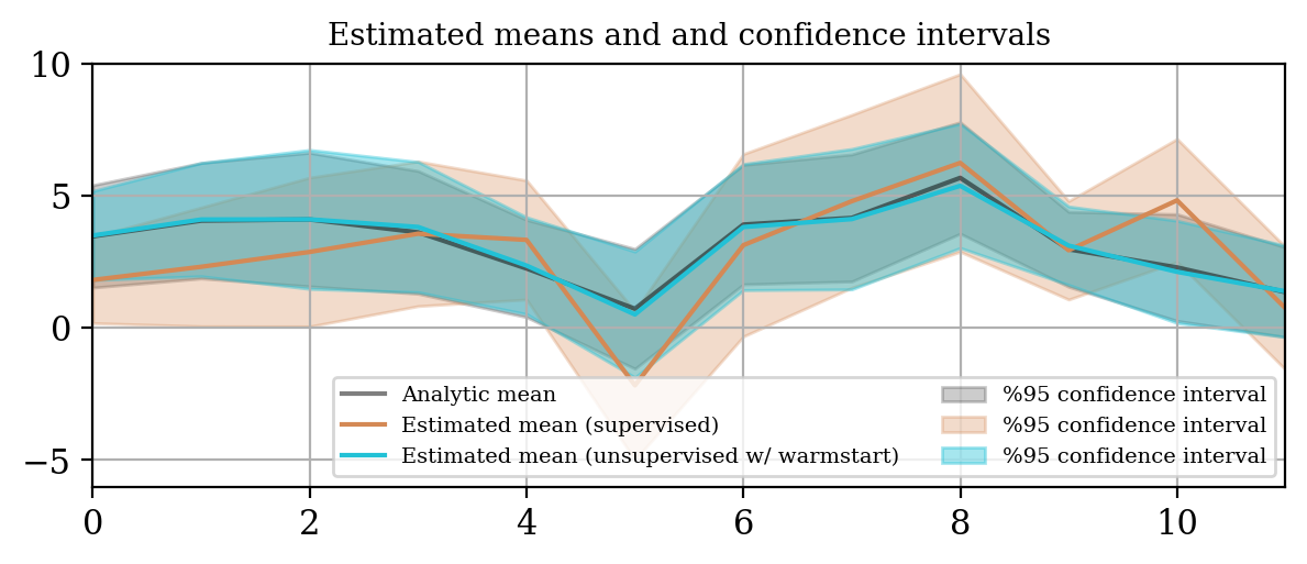
(a)

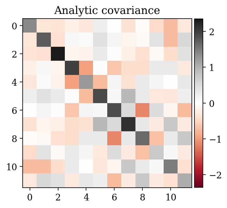
(b)

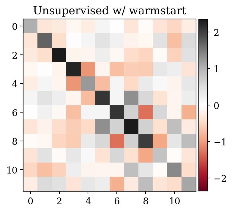
(c)

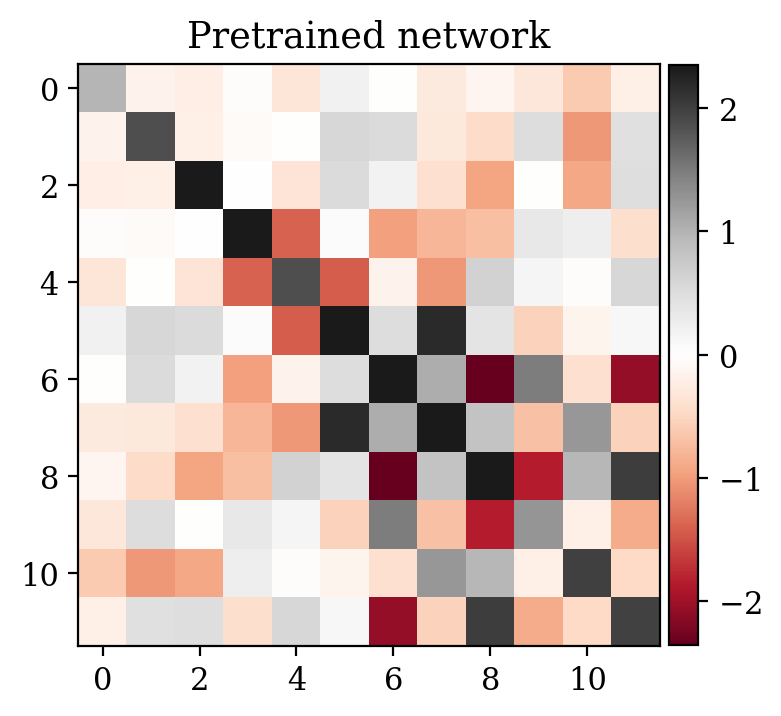
(d)

Figure 1: Comparison of the posterior mean (a) and covariance (b–d) obtained from supervised and unsupervised training for the Gaussian problem. Note that the results are supposed to differ, due to different prior and observation models. The analytic mean and covariance here refers to the unsupervised problem.

We study the convergence history for unsupervised training with and without warm start, as described in Equation (9). The plot in Figure 2 makes clear the computational superiority of the warm start approach.

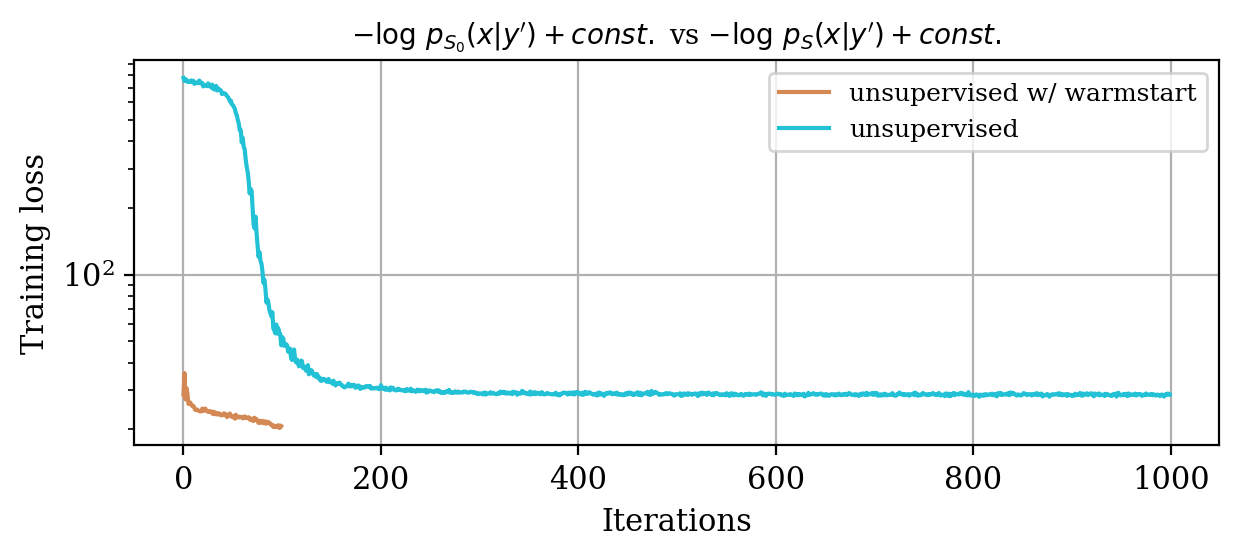
Figure 2: Loss decay for the unsupervised Gaussian problem as a function of iterations. The comparison highlights the efficiency of the warm start strategy compared to training from scratch.

4.2 Seismic images

Now we consider the denoising problem for 2D “seismic” images $x$, which are selected from the processed 3D seismic survey reported in Veritas [20] and WesternGeco. [21]. The dataset has been obtained by selecting 2D patches from the original 3D volume, which are then subsampled in order to obtain $64\times 64$ pixel images. The dataset is normalized.

Observations $y$ are obtained simply by adding noise

$$y=x+\varepsilon,\quad\varepsilon\sim\mathcal{N}(\mu_{\varepsilon},\Sigma_{\varepsilon})$$ (13)

with $\mu_{\varepsilon}=0$ and $\Sigma_{\varepsilon}=1.2\,I$. Examples of $(x,y)$ pairs are collected in Figure 3. As in the previous examples, we consider a preliminary stage for supervised training via conditional normalizing flows.

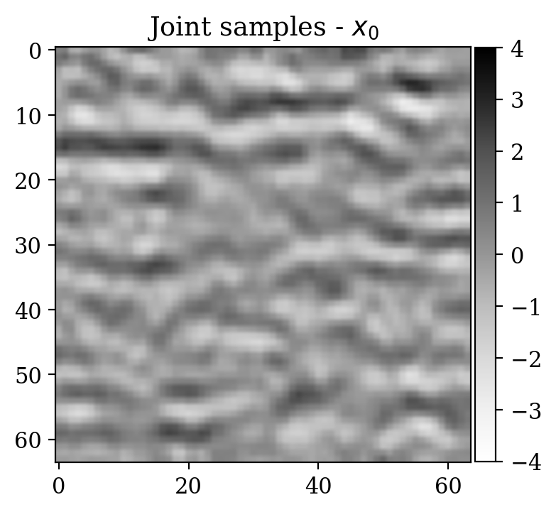
(a)

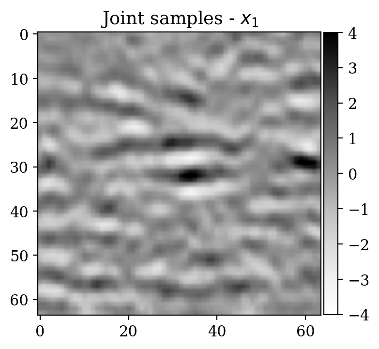
(b)

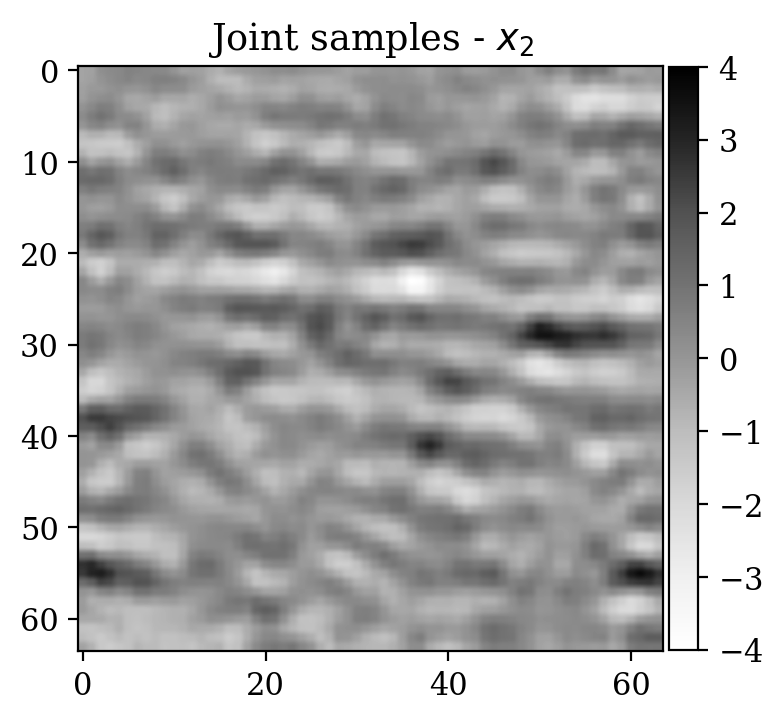
(c)

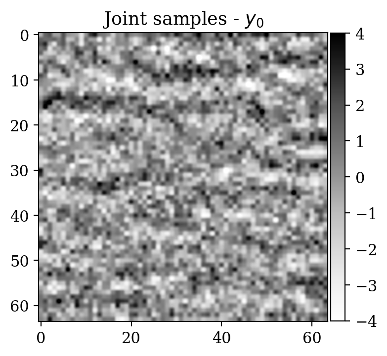
(d)

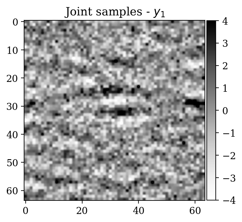
(e)

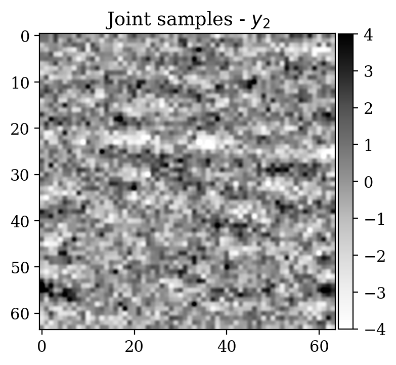
(f)

Figure 3: Unknown and observation pairs $(x,y)$ for the supervised seismic image problem (first row: $x$, second row: $y$).

We now turn to the unsupervised problem defined by the observation likelihood

$$y^{\prime}=A\,x^{\prime}+\varepsilon^{\prime},\quad\varepsilon^{\prime}\sim\mathcal{N}(\mu_{\varepsilon^{\prime}},\Sigma_{\varepsilon^{\prime}})$$ (14)

with $\mu_{\varepsilon^{\prime}}=0$ and $\Sigma_{\varepsilon^{\prime}}=0.2\,I$. Note that a forward operator $A$ has been introduced, contrary to Equation (13). Here, $A$ is equal to $B^{T}B$, where $B$ is a compressing sensing matrix with $30\%$ subsampling rate. The ground truth $x^{\prime}$ for observations $y^{\prime}$ has been selected from a test set not contemplated during the supervised training phase. As a prior for $x^{\prime}$, we select the posterior distribution given $y^{\prime}$ which has been pretrained with supervision in the previous step (see Equation (4)).

Again, comparing the loss decay during training for two different instances of the unsupervised problem in Figure 4, makes clear that considerable speed up is obtained with the warm start strategy relatively to training a randomly initialized invertible network.

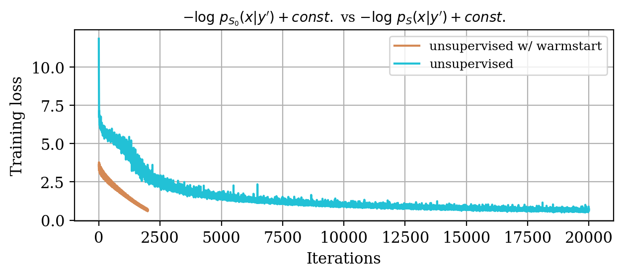
(a)

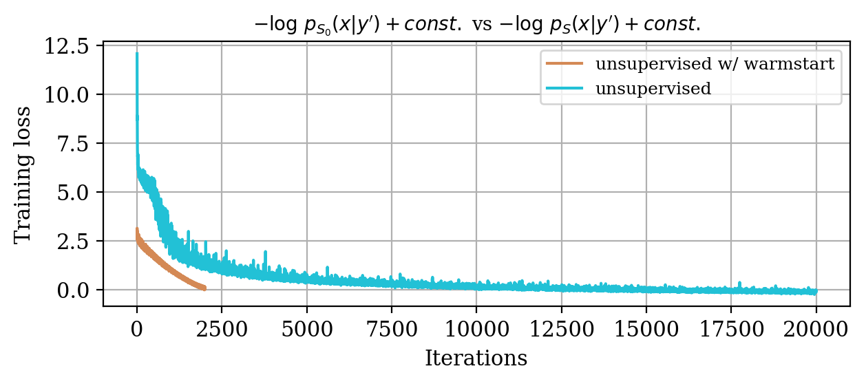
(b)

Figure 4: Loss decays for two different instances of the unsupervised problems related to seismic images. As in the previous example, training with a warm start strategy evidently requires less iterations than training from scratch in order to reach the same loss value.

Moreover, despite the relatively high number of iterations ran during training ($\sim 20000$), the network initialized from scratch does not produce a reasonable result comparable to the ground truth. This can be seen by comparing the ground truth in Figure 6a and the conditional mean in Figure 6e, relative to the posterior distribution obtained from training a network from scratch. The comparison with the ground truth is much more favorable with the conditional mean obtained from the warm start training, in Figure 6c. Pointwise standard deviations for these different training modalities can also be inspected in Figures 6d (warm start) and 6f (without warm start). The discussed results above are related to the loss function depicted in Figure 4a. Same results for a different realization of the unsupervised problem with loss function shown in Figure 4b can be seen in Figure 6.

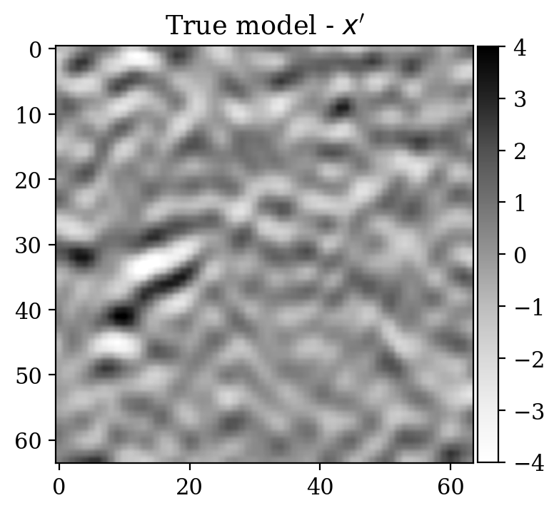
(a)

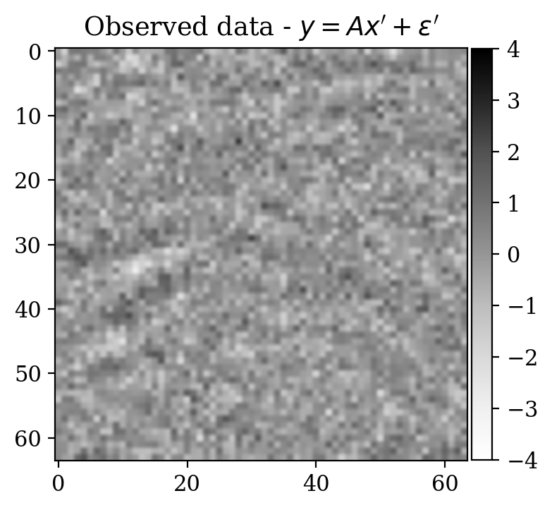
(b)

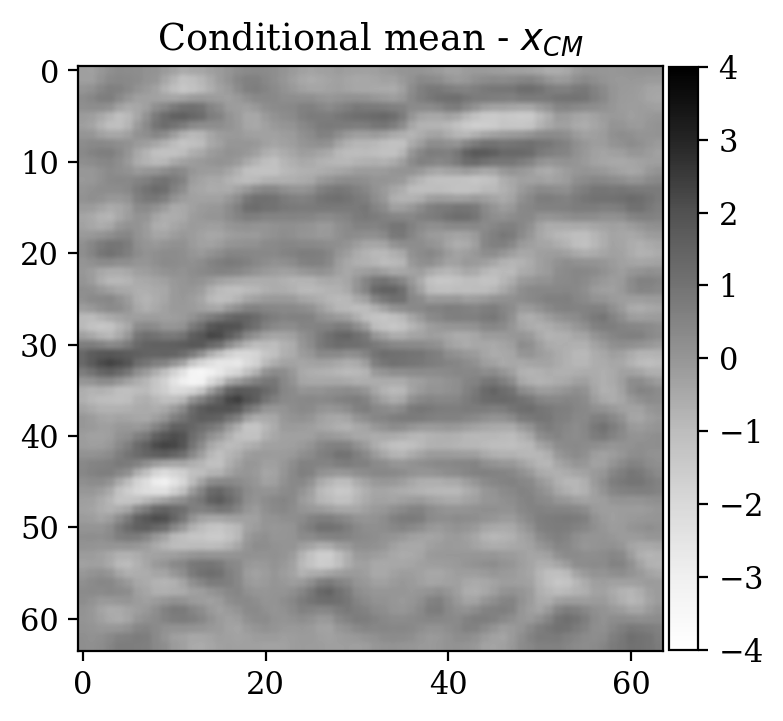
(c)

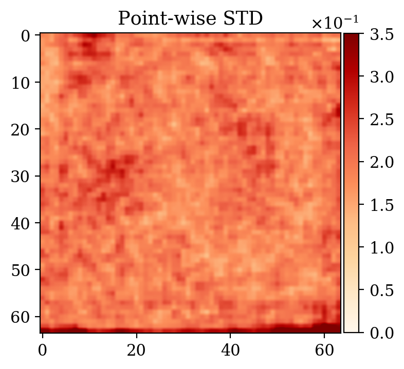
(d)

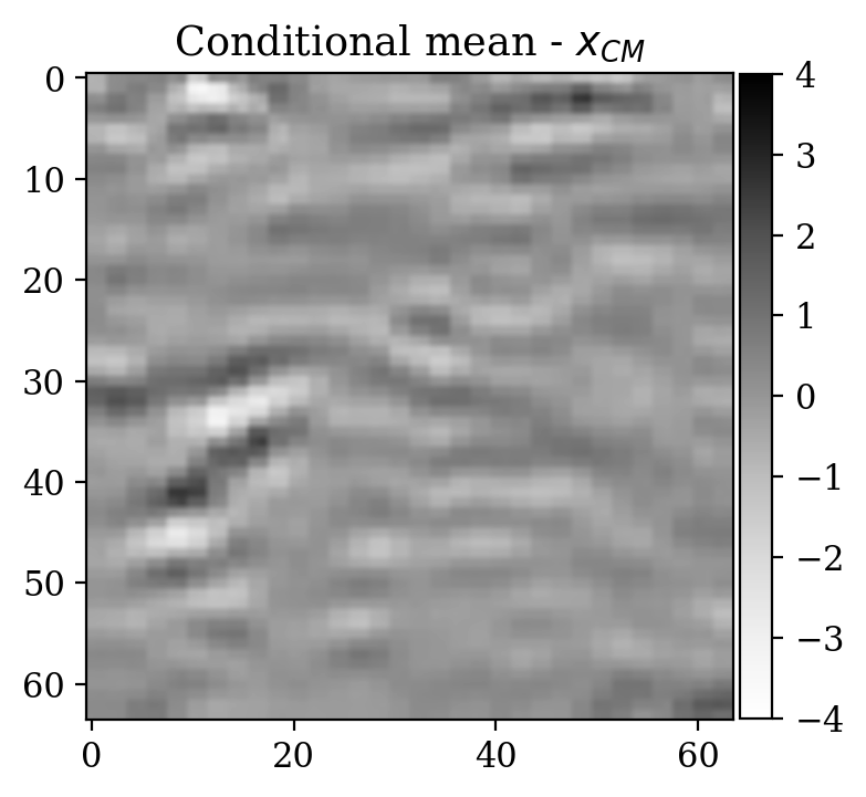
(e)

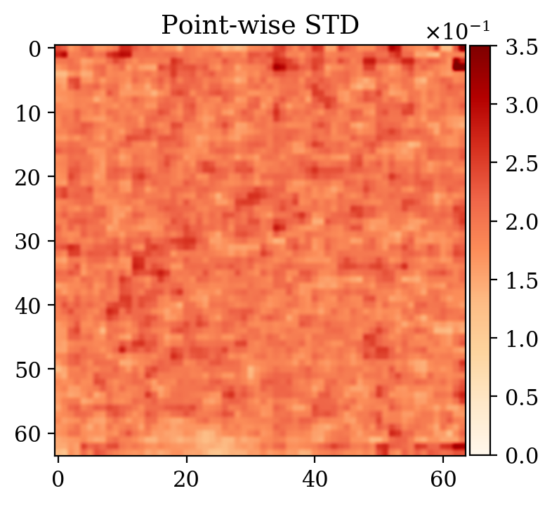
(f)

Figure 5: Comparison of the posterior distribution obtained from training a network with warm start and from scratch for the unsupervised seismic image problem. Figures (a) and (b) depict the ground truth and related observations. Figures (c) and (e) represent the respective conditional means, while (d) and (f) refer to the pointwise standard deviation. Note how the result in (c) provides a better estimation of the ground truth (a) compared to (e).

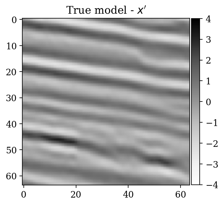
(a)

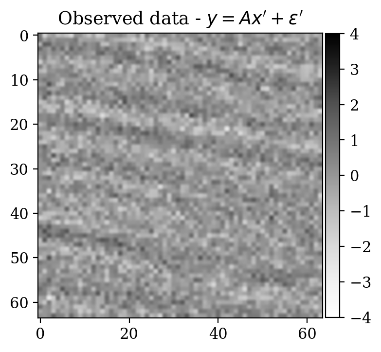
(b)

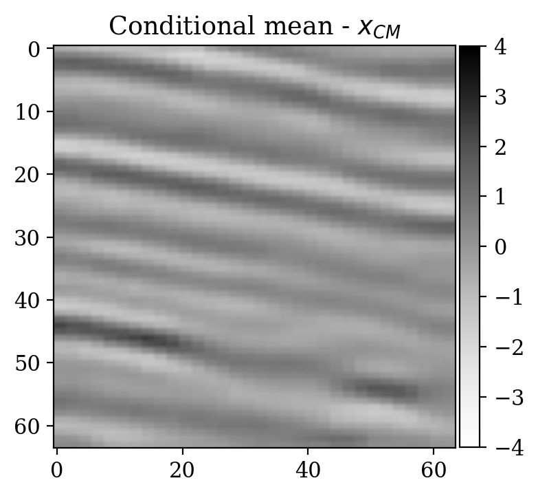
(c)

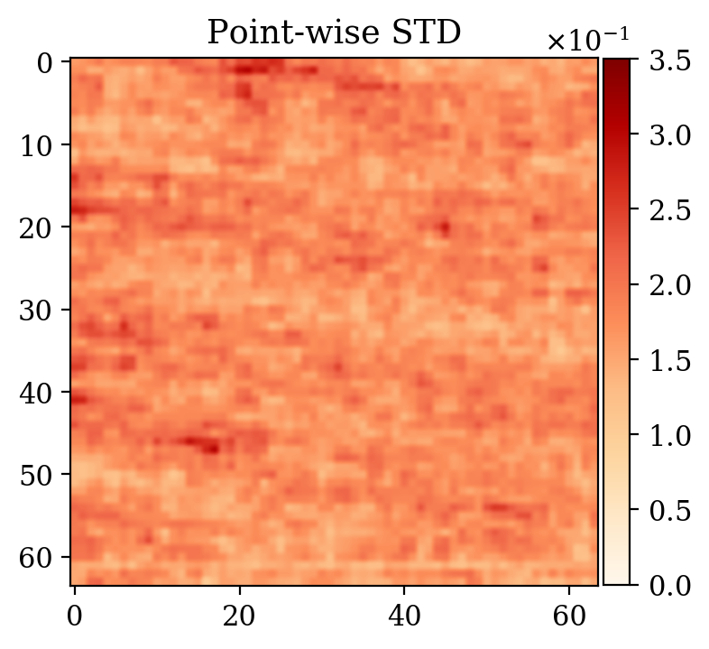
(d)

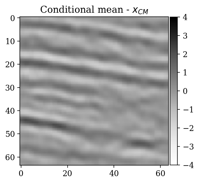
(e)

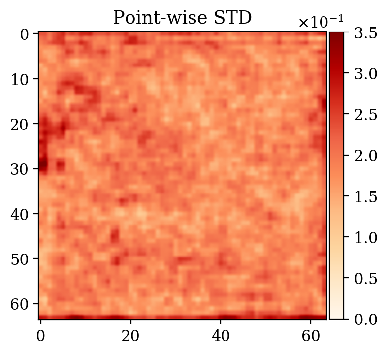
(f)

Figure 6: Comparison of the posterior distribution obtained from training a network with warm start and from scratch for the unsupervised seismic image problem. Figures (a) and (b) depict the ground truth and related observations. Figures (c) and (e) represent the respective conditional means, while (d) and (f) refer to the pointwise standard deviation. Note how the result in (c) provides a better estimation of the ground truth (a) compared to (e).

5 Conclusions

We presented a preconditioning scheme for uncertainty quantification, particularly aimed at inverse problems characterized by computationally expensive numerical simulations based on PDEs (including, for example, seismic or optoacoustic imaging). We consider the problem where legacy supervised data is available, and we want to solve for a new inverse problem given some out-of-distribution observations. The scheme takes advantage of a preliminary step where the joint distribution of solution and related observations is learned via supervised learning. This joint distribution is then employed as a way to precondition the unsupervised inverse problem. In the supervised and unsupervised case, we make use of conditional normalizing flows to ease computational complexity (fundamental for large 3D applications), and to be able to encode analytically the approximated posterior density. In this way, the posterior density obtained from the supervised problem can be reused as a new prior for the unsupervised problem.

The synthetic experiments confirm that the preconditioning scheme accelerates unsupervised training considerably. The examples here considered are encouraging for seismic or optoacoustic imaging applications, but additional challenges are expected for large scales due to the high dimensionality of the solution and observation space, and expensive wave equation solvers.

References

- Adler and Öktem [2017] Jonas Adler and Ozan Öktem. Solving ill-posed inverse problems using iterative deep neural networks. Inverse Problems, 33(12):124007, Nov 2017. ISSN 1361-6420. doi: 10.1088/1361-6420/aa9581. URL http://dx.doi.org/10.1088/1361-6420/aa9581.
- Bora et al. [2017] Ashish Bora, Ajil Jalal, Eric Price, and Alexandros G. Dimakis. Compressed sensing using generative models, 2017.
- Ulyanov et al. [2020] Dmitry Ulyanov, Andrea Vedaldi, and Victor Lempitsky. Deep image prior. International Journal of Computer Vision, Mar 2020. ISSN 1573-1405. doi: 10.1007/s11263-020-01303-4. URL http://dx.doi.org/10.1007/s11263-020-01303-4.
- Herrmann et al. [2019] F. J. Herrmann, A. Siahkoohi, and G. Rizzuti. Learned imaging with constraints and uncertainty quantification. In Neural Information Processing Systems (NeurIPS) 2019 Deep Inverse Workshop, 12 2019. URL https://arxiv.org/pdf/1909.06473.pdf.
- Siahkoohi et al. [2020a] Ali Siahkoohi, Gabrio Rizzuti, and Felix J. Herrmann. A deep-learning based bayesian approach to seismic imaging and uncertainty quantification. In 82nd EAGE Conference and Exhibition 2020, 2020a. URL https://arxiv.org/pdf/2001.04567.pdf.
- Siahkoohi et al. [2020b] Ali Siahkoohi, Gabrio Rizzuti, and Felix J. Herrmann. Weak deep priors for seismic imaging. In SEG Technical Program Expanded Abstracts 2020, 2020b. URL https://arxiv.org/pdf/2004.06835.pdf.
- Siahkoohi et al. [2020c] Ali Siahkoohi, Gabrio Rizzuti, and Felix J. Herrmann. Uncertainty quantification in imaging and automatic horizon tracking—a bayesian deep-prior based approach. In SEG Technical Program Expanded Abstracts 2020, 2020c. URL https://arxiv.org/pdf/2004.00227.pdf.
- Kruse et al. [2019] J. Kruse, G. Detommaso, R. Scheichl, and U. Köthe. HINT: Hierarchical Invertible Neural Transport for Density Estimation and Bayesian Inference, 2019.
- Winkler et al. [2019] Christina Winkler, Daniel Worrall, Emiel Hoogeboom, and Max Welling. Learning likelihoods with conditional normalizing flows, 2019.
- Dinh et al. [2014] Laurent Dinh, David Krueger, and Yoshua Bengio. Nice: Non-linear independent components estimation, 2014.
- Dinh et al. [2016] L. Dinh, J. Sohl-Dickstein, and S. Bengio. Density estimation using Real NVP, 2016.
- Kingma and Dhariwal [2018] D. P. Kingma and P. Dhariwal. Glow: Generative Flow with Invertible 1x1 Convolutions, 2018.
- Peters et al. [2020] Bas Peters, Eldad Haber, and Keegan Lensink. Fully reversible neural networks for large-scale surface and sub-surface characterization via remote sensing. arXiv preprint arXiv:2003.07474, 2020.
- Rizzuti et al. [2020] Gabrio Rizzuti, Ali Siahkoohi, Philipp A. Witte, and Felix J. Herrmann. Parameterizing uncertainty by deep invertible networks, an application to reservoir characterization. In SEG Technical Program Expanded Abstracts 2020, 2020. URL https://arxiv.org/pdf/2004.07871.pdf.
- Putzky and Welling [2019] P. Putzky and M. Welling. Invert to Learn to Invert, 2019.
- Parno and Marzouk [2018] M. D. Parno and Y. M. Marzouk. Transport Map Accelerated Markov Chain Monte Carlo. SIAM/ASA Journal on Uncertainty Quantification, 6(2):645–682, 2018. doi: 10.1137/17M1134640.
- Peherstorfer and Marzouk [2018] Benjamin Peherstorfer and Youssef Marzouk. A transport-based multifidelity preconditioner for Markov chain Monte Carlo, 2018.
- Yosinski et al. [2014] Jason Yosinski, Jeff Clune, Yoshua Bengio, and Hod Lipson. How transferable are features in deep neural networks? In Proceedings of the 27th International Conference on Neural Information Processing Systems, NIPS’14, pages 3320–3328, 2014. URL http://dl.acm.org/citation.cfm?id=2969033.2969197.
- Siahkoohi et al. [2019] A. Siahkoohi, M. Louboutin, and F. J. Herrmann. The importance of transfer learning in seismic modeling and imaging. Geophysics, 84(6):A47–A52, 11 2019. doi: 10.1190/geo2019-0056.1.
- Veritas [2005] Veritas. Parihaka 3D Marine Seismic Survey - Acquisition and Processing Report. Technical Report New Zealand Petroleum Report 3460, New Zealand Petroleum & Minerals, Wellington, 2005.
- WesternGeco. [2012] WesternGeco. Parihaka 3D PSTM Final Processing Report. Technical Report New Zealand Petroleum Report 4582, New Zealand Petroleum & Minerals, Wellington, 2012.