Local time of infinite time horizon Brownian bridge

Abstract

We introduce an infinite time horizon Brownian bridge which is determined by a stochastic Langevin equation with time dependent drift coefficient. We show that this process goes to zero almost surely when the time goes to infinity and study the existence and asymptotic behavior of its local time as well as its Hölder continuity in time variable and in location variable. The main difficulty is the lack of stationarity of the process so that the powerful tools for stationary (Gaussian) processes are not applicable. We employ the Garsia-Rodemich-Rumsey inequality to get around this type of difficulty.

1 Introduction

The Markov bridge is widely used in statistics, probability and finance. For example, in statistics Brownian bridge plays an important role in the Kolmogorov-Smirnov test. In the probability theory, it is well-known that Brownian, Gamma and Bessel bridges have been developed extensively in the literature (see e.g., [5, 13, 22]) and references therein. By means of $h$-function, some general Markov bridges with the SDE representation on $[0,T]$ were constructed in [9]. In finance the $\alpha$-Brownian bridge was used in [7] to model the arbitrage profit associated with a given futures contract. The phenomenon of stock pinning on option expiration dates was described via the bridge in [1]. Markov bridges are also employed to solve the famous insider trading Kyle-Back models (cf. [3, 19] and many references which follow). There are many other studies and applications of Markov bridges, we refer to e.g. [10] and the references therein.

On a complete filtration probability space $\Lambda:=(\Omega,\mathbb{P},\mathcal{F}_{t},\mathcal{F})$, a $\alpha$-Brownian bridge on the interval $[0,T]$ is defined by

$$\left\{\begin{aligned} &dX_{t}=\frac{-\alpha X_{t}}{T-t}dt+dW_{t}\;,&t\in[0,T),\\ &X_{0}=0,\end{aligned}\right.$$ (1.1)

where $\alpha>0$, $T\in(0,\infty)$, and $\{W_{t}\}_{t\geq 0}$ is a standard Brownian motion on $(\Omega,\mathbb{P},\mathcal{F}_{t},\mathcal{F})$. If $\alpha=1$, $\{X_{t}\}_{t\geq 0}$ is the standard Brownian bridge. There is also a vast literature on the property of this type of Brownian bridge and its application, including local time and stopping time (cf. [6, 11, 12, 21, 24]).

In application, sometime we don’t specify the terminal time $T$. For example, in the optimal portfolio and consumption problem in mathematical finance, sometimes it is more desirable to consider the optimal portfolio problem for an individual’s life time, which is not a priori determined. Sometime the terminal time $T$ we are concerned is large. In this case it is convenient to use the Brownian bridge over an infinite time horizon. Although [10] provided the weak condition of Markov bridges with $T=\infty$, it is still in the framework of SDE containing parameter $T$. To the best of our knowledge, there is no reference concerning Brownian bridge in the case $T=\infty$.

To construct such an infinite time horizon Brownian bridge, we cannot simply let the drift term $b_{T}(t,x)=-\frac{\alpha x}{T-t}$ in (1.1) go to infinite since it simply goes to zero, which yields the Brownian motion. On the other hand, if the drift term is $-\alpha x$ then the solution $X_{t}$ is the famous time-homogeneous OU process, which has a (non zero) limit as $t\rightarrow\infty$. This motivates us to require the drift to have the form $b(t,x)=-\alpha(t)x$ such that $\alpha(t)\rightarrow\infty$ when $t\rightarrow\infty$. Thus, in this paper we deal with the general Brownian bridge on an infinite time horizon satisfying the following stochastic differential equation (SDE):

$$\left\{\begin{aligned} &dX_{t}=-\alpha(t)X_{t}dt+dW_{t}\;,&t\in[0,\infty),\\ &X_{0}=0,\end{aligned}\right.$$ (1.2)

where $\alpha(t)$ is a deterministic function. This equation can be easily modified to construct more general Brownian bridge $X_{t}^{a,b}$ starting at $X_{0}^{a,b}=a$ and terminating at $X_{\infty}^{a,b}=b$:

$$\left\{\begin{aligned} &dX_{t}^{a,b}=-\alpha(t)(X_{t}^{a,b}-b)dt+dW_{t}\;,&t\in[0,\infty),\\ &X_{0}^{a,b}=a,\end{aligned}\right.$$ (1.3)

since the solutions to the above equations (1.2) and (1.3) are related by

$$X_{t}^{a,b}=b+(a-b)e^{-\int_{0}^{t}\alpha(r)dr}+X_{t}\,.$$

After proposing the candidate (1.2) for the infinite time horizon Brownian bridge the first task is to show we do indeed have $\displaystyle\lim_{t\rightarrow\infty}X_{t}=0$ almost surely. In the classical case of finite time horizon, the terminal pinning point almost surely limit $\displaystyle\lim_{t\to T}X_{t}=0$ can be proved by the strong law of large numbers for Brownian motion (cf. [17, Page 359]). However, it cannot be conducted in our case because of $T=\infty$ and because of the explosive behavior of the drift term $\alpha(t)$. In general, since an important feature of the process $X_{t}$ is that it is no longer stationary, many powerful tools effective for stationary process is no longer applicable and we need completely different probabilistic techniques.

Our strategy to prove the bridge property of $\displaystyle\lim_{t\to\infty}X_{t}=0$ almost surely is first to prove $\displaystyle\lim_{n\to\infty}X_{n}=0$ almost surely along positive integers $\mathbb{N}$ by using some moment estimates and the Borel-Cantelli lemma. The main difficulty lays in the case of continuous time. We find that the Garsia-Rodemich-Rumsey inequality can play a crucial role. This is done in Section 2.

To study a stochastic process, an important concept is its local time. For standard Brownian motions there are many works and here we only refer to [20]. Since our Brownian bridge is defined on the half line $\mathbb{R}_{+}$, we are first concerned with the asymptotic behavior of the local time ${\cal L}_{t}^{x}=\int_{0}^{t}{\delta}(X_{s}-x)ds$ as $t\rightarrow\infty$. We show the existence of the local time and we show $\displaystyle\lim_{t\rightarrow\infty}{\cal L}_{t}^{x}=\infty$ under some minor restrictions on $\alpha(t)$ in Section 3.

The Hölder continuity of the local time has been well-studied for Brownian motion and other processes (cf. [2, 20] and references therein). We shall also study this property for our local time of the Brownian bridge. Again since the local time can be defined for all $t\in\mathbb{R}_{+}$ and $x\in\mathbb{R}$, it is interesting to know how the Hölder coefficient depends on the size of the domain. For the Hölder continuity on time variable, we shall give a positive answer. More precisely, we shall prove that there is a finite random constant $C$, independent of $s,t,T$, such that $|{\cal L}_{t}^{x}-{\cal L}_{s}^{x}|\leq C\left[|t-s|^{1/2}\sqrt{(T+1)\alpha^{*}(T+1)}+|t-s|^{1/2}\sqrt{\log\frac{1}{|t-s|}}\ \right]$,  $\forall\ 0\leq s,t\leq T<\infty$. This will need some nondeterminism results for the Brownian bridge process. Compared with the result of [18] this result is sharp on any bounded interval. But for the Hölder continuity with respect to location parameter we can only show that its Hölder exponent can arbitrarily close to $1/2$. This is done in Section 4. In section 5, we give some numerical experiments on a typical sample path of an infinite time horizon Brownian bridge.

The infinite time horizon Brownian bridge process is a special case of time-dependent modulated drift Ornstein-Uhlenbeck (OU) processes, which is popular for modeling the evolution of interest rate (cf. [8, 16]). From a theoretical point of view, it is also interesting to know that the time-dependent OU process becomes an infinite time horizon bridge process when the drift term has some growth rate.

2 Infinite time horizon Brownian bridges

In this section, we provide a sufficient condition on the drift coefficient $\alpha(t)$ in Equation (1.2) so that $X_{\infty}=0$ (more precisely $\displaystyle\lim_{t\rightarrow\infty}X_{t}=0$ almost surely). Namely, we provide a sufficient condition so that we have an infinite time horizon Brownian bridge: a mean zero Gaussian process $(X_{t},0\leq t\leq\infty)$ such that $X_{0}=X_{\infty}=0$. It worths to point out that such process is not unique as we shall see and from the construction (see Equation (2.1) below), the Brownian bridge is adapted to the Brownian motion $W$. The main techniques that we need are Garsia-Rodemich-Rumsey inequality and Borel-Cantelli lemma. First we have the following representation of the solution to (1.2).

Proposition 2.1

The SDE (1.2) has a unique strong solution given by

$$X_{t}=\int_{0}^{t}\exp\left(-\int_{s}^{t}\alpha(u)du\right)dW_{s},\quad 0\leq t<\infty.$$ (2.1)

Proof 1

Since for $0\leq t<\infty$, $-\alpha(t)$ satisfies the usual Lipschitz and linear growth conditions, the SDE (1.2) has a unique strong solution (see e.g. [17, Section 5]). By Itô’s formula, it is easy to verify that the process $X_{t}$ defined by equation (2.1) is the solution to (1.2).

Next, we define

$$X_{t}:=\left\{\begin{aligned} &\int_{0}^{t}\exp\left(-\int_{s}^{t}\alpha(u)du\right)dW_{s},&t<\infty,\\ &0,&t=\infty\,.\end{aligned}\right.$$ (2.2)

For convenience of notations, throughout this paper we shall use $C$ to denote a generic finite positive constant, whose value may be different in different appearances. When we need to stress the dependence of a constant on ${\gamma}$, we use $C_{\gamma}$, whose values may also be different in different appearances. For a function $\alpha(t):[0,\infty)\to\mathbb{R}$ we introduce the following notation:

$$\alpha^{*}(t):=\sup_{0\leq r\leq t}\alpha(r)\,,\quad 0\leq t<\infty\,.$$ (2.3)

Theorem 2.1

Let the time-dependent coefficient function $\alpha(t):[0,\infty)\to\mathbb{R}^{+}$ be continuously differentiable and satisfy the following growth condition:

1. There are ${\gamma}\in[0,1/2]$ and $\beta>0$ such that $\frac{(\alpha^{*}(t+1))^{2{\gamma}}}{\alpha(t)}\leq Ct^{-\beta}$ for all $0\leq t<\infty$.

2. There is a constant $C$ such that $\sup_{t\geq 0}|\frac{\alpha^{\prime}(t)}{\alpha(t)}|\leq C$.

Then the process $\{X_{t}\}_{t\geq 0}$ defined by (2.2) is a centered Gaussian process with almost surely continuous sample paths on the closed infinite time horizon $[0,\infty]$.

Remark 2.1

1. Condition (i) implies that

   $$\alpha(t)\geq C_{\beta}t^{\beta}\,,\quad\forall\ 0\leq t<\infty\,.$$ (2.4)

2. The condition (i) in Theorem 2.1 can be replaced by “there are $t_{0}>0$, ${\gamma}\in[0,1/2]$, $\beta>0$, and $K>0$ such that $\frac{(\alpha^{*}(t+K))^{2{\gamma}}}{\alpha(t)}\leq Ct^{-\beta}$ for all $t_{0}\leq t<\infty$”.

3. The condition that $\alpha(t)\rightarrow\infty$ seems necessary. For example if $\alpha(t)=\alpha$ is a constant function, the process $X_{t}$ will be a usual OU process, which converges to a nondegenerate Gaussian random variable.

To prove this theorem, we need the following three lemmas, whose proofs are given in A

Lemma 2.1

Assume that the function $g:[0,\infty)\to\mathbb{R}^{+}$ is continuous and satisfies $\lim_{x\rightarrow+\infty}g(x)=+\infty$. If there is a positive constant $C$ such that $\sup_{x>0}|\frac{g^{\prime}(x)}{g(x)}|\leq C$, then for any $\kappa>0$, there are positive constants $x_{0}$, $\bar{C}_{\kappa,g}$, and $C_{\kappa,g}$, independent of $x\in\mathbb{R}_{+}$, such that for all $x>x_{0}$,

$$\bar{C}_{\kappa,g}\leq\frac{g(x)\int_{0}^{x}\exp\left(\kappa\int_{0}^{s}g(u)du\right)ds}{\exp\left(\kappa\int_{0}^{x}g(u)du\right)}\leq C_{\kappa,g}\,,$$ (2.5)

Lemma 2.2

Let $X$ be the solution to (1.2) and $\alpha(t)$ satisfy the conditions in Theorem 2.1. Then for any ${\gamma}\in[0,1/2]$ and for any $t_{1},t_{2}>0$,

$$\sigma^{2}_{t_{1},t_{2}} :=\mathbb{E}|X_{t_{2}}-X_{t_{1}}|^{2}$$

$$\leq C_{{\gamma}}|{t_{2}}-{t_{1}}|^{2{\gamma}}\left[\left(\alpha^{*}(t_{1}\vee t_{2})\right)^{2{\gamma}}(\alpha(t_{1}\wedge t_{2}))^{-1}+(\alpha(t_{1}\vee t_{2}))^{2{\gamma}-1}\right]\,.$$ (2.6)

Example 2.1

If there is a $t_{0}>0$ such that for all $t>t_{0}$, $\alpha(t)\geq Ct^{{\beta}}$ for some ${\beta}>0$ and $\alpha(t)\leq Ct^{p}$ for some ${\beta}\leq p<\infty$, and if $t_{0}<t_{1}<t_{2}<t_{1}+1$, then

$$\sigma^{2}_{t_{1},t_{2}} \leq C_{{\gamma}}\left|t_{2}-t_{1}\right|^{2{\gamma}}\left[\left(t_{1}+1\right)^{2{\gamma}p}t_{1}^{-{\beta}}+(t_{1})^{-\beta(1-2{\gamma})}\right]$$

$$\leq C_{{\gamma}}\left|t_{2}-t_{1}\right|^{2{\gamma}}t_{1}^{-\rho}$$

for some $\rho\in(0,{\beta})$ when ${\gamma}>0$ is sufficiently small. We can also assume that $\alpha(t)>e^{pt}$ and $\alpha(t)\leq e^{qt}$ for some positive constants $p$ and $q$.

Lemma 2.3

Let $\beta>0$, ${\gamma}\in[0,1/2]$. Fix an arbitrary positive number $N>1$. Choose a positive integer $m$ such that $m{\gamma}>2$, $2N/m<\beta$, $2{\gamma}<1-2N/(\beta m)$. Assume that the conditions in Theorem 2.1 are satisfied. Then, there is a random constant $R_{N,m}$ (independent of $k$) such that for any integer $k\geq 1$, $t_{1},t_{2}\in[k,k+1]$, the following inequality holds.

$$|X_{t_{2}}-X_{t_{1}}|\leq R_{N,m}C_{\gamma}k^{-\beta\left[1-2{\gamma}-2N/(\beta m)\right]/2}\,.$$ (2.7)

Now we are ready to prove Theorem 2.1.

Proof of Theorem 2.1 1

First, we show $\lim_{n\rightarrow\infty}X_{n}=0$ along the positive integers. For any real number $\epsilon>0$, any positive integer $q$ with ${\beta}q>1$, by the Chebyshev’s inequality and then by Lemma 2.1, we have

$$\sum_{k=1}^{\infty}\mathbb{P}(|X_{k}|>\epsilon) \leq\sum_{k=1}^{\infty}\frac{\mathbb{E}|X_{k}|^{2q}}{\epsilon^{2q}}$$

$$\leq\sum_{k=1}^{\infty}\frac{M_{q}\left(\int_{0}^{k}\exp\left(-\int_{s}^{k}2\alpha(u)du\right)ds\right)^{q}}{\epsilon^{2q}}$$

$$\leq\sum_{k=1}^{\infty}\frac{C_{q}}{\epsilon^{2q}\left(\alpha(k)\right)^{q}}\leq\sum_{k=1}^{\infty}\frac{C_{q}}{\epsilon^{2q}k^{{\beta}q}}<\infty,$$

where $M_{p}=\frac{(2q)!}{2^{q}(q)!}$ . Then the Borel-Cantelli lemma implies $\mathbb{P}(|X_{k}|>\epsilon~{}\textup{i.o.})=0$. Since $\epsilon$ is arbitrary, then $X_{k}$ converges to zero almost surely as $k\to\infty$.

Next, we will show the almost sure convergence result for continuous time, namely, we need to show $X_{t}$ converges to zero almost surely as $t\to\infty$. Clearly, we have

$$|X_{t}|\leq|X_{t}-X_{k}|+|X_{k}|,$$ (2.8)

where $k=\lfloor t\rfloor$ is the biggest integer less than or equal to the real number $t$. The second term in (2.8) converges to zero almost surely as $k=\lfloor t\rfloor\to\infty$ from the previous argument. Lemma 2.3 can be used to show that the first term in equation (2.8) also converges to zero almost surely as $t\to\infty$.

3 Local time of infinite time horizon Brownian bridges

In this section, we study the local time for the infinite time horizon Brownian bridges. The local time of the one-dimensional infinite time horizon Brownian bridge $\{X_{t}\}_{t\geq 0}$ at level $x$ is defined by

$$\mathcal{L}_{t}^{x}=\int_{0}^{t}\delta(X_{r}-x)dr,$$ (3.1)

which is the limit (in $L^{2}$ if the limit exists) of the approximating local time process defined by

$$\mathcal{L}_{t,\varepsilon}^{x}=\lim_{\varepsilon\to 0+}\int_{0}^{t}p_{\varepsilon}(X_{r}-x)dr,$$ (3.2)

where $\delta(\cdot)$ is the Dirac delta function at zero, $p_{\varepsilon}(x)=\frac{1}{\sqrt{2\pi\varepsilon}}\exp\left(-\frac{x^{2}}{2\varepsilon}\right)$ is the heat kernel with $\varepsilon>0$. To study the limit of $\mathcal{L}_{t,\varepsilon}^{x}$ we use the following representation for the heat kernel:

$$p_{\varepsilon}(x)=\frac{1}{2\pi}\int_{\mathbb{R}}\exp\left(i\xi x-\frac{\varepsilon\xi^{2}}{2}\right)d\xi,$$ (3.3)

where $i^{2}=-1$.

Lemma 3.1

For any $x\in\mathbb{R}$, $0<t<\infty$, we have

$$\lim_{\varepsilon,\theta\to 0+}\mathbb{E}|\mathcal{L}_{t,\varepsilon}^{x}-\mathcal{L}_{t,\theta}^{x}|^{2}=0.$$

Proof 2

To simplify notation, and without loss of generality we will assume $x=0$ in the following argument for the existence of the limit. We set $\mathcal{L}_{t}=\mathcal{L}_{t}^{0}$ and $\mathcal{L}_{t,\varepsilon}=\mathcal{L}_{t,\varepsilon}^{0}$. Since $\mathbb{E}|\mathcal{L}_{t,\varepsilon}-\mathcal{L}_{t,\theta}|^{2}=\mathbb{E}(\mathcal{L}_{t,\varepsilon})^{2}+\mathbb{E}(\mathcal{L}_{t,\theta})^{2}-2\mathbb{E}(\mathcal{L}_{t,\varepsilon}\mathcal{L}_{t,\theta})$, we only need to compute $\mathbb{E}(\mathcal{L}_{t,\varepsilon}\mathcal{L}_{t,\theta})$. We use the expression (3.3) for this computation:

$$\mathbb{E}(\mathcal{L}_{t,\varepsilon}\mathcal{L}_{t,\theta}) =\frac{1}{4\pi^{2}}\int_{0}^{t}\int_{0}^{t}\int_{\mathbb{R}^{2}}\mathbb{E}\left\{\exp\left(i(\xi X_{r}+\eta X_{s})-\frac{\varepsilon\xi^{2}+\theta\eta^{2})}{2}\right)\right\}d\xi d\eta dsdr$$

$$=\frac{1}{4\pi^{2}}\int_{0}^{t}\int_{0}^{t}\int_{\mathbb{R}^{2}}\left\{\exp\left(-\frac{1}{2}E\left[\xi X_{r}+\eta X_{s}\right]^{2}-\frac{\varepsilon\xi^{2}+\theta\eta^{2})}{2}\right)\right\}d\xi d\eta dsdr$$

$$=\frac{1}{2\pi}\int_{0}^{t}\int_{0}^{t}\left[{\rm det}(A_{\varepsilon,\theta}(s,r))\right]^{-1/2}dsdr$$

$$=\frac{1}{\pi}\int_{0}^{t}\int_{0}^{s}\left[{\rm det}(A_{\varepsilon,\theta}(s,r))\right]^{-1/2}drds,$$

where

$$A_{\varepsilon,\theta}(s,r)=\begin{pmatrix}\mathbb{E}(X_{s}^{2})+\theta&\mathbb{E}(X_{r}X_{s})\\ \mathbb{E}(X_{r}X_{s})&\mathbb{E}(X_{r}^{2})+\varepsilon\\ \end{pmatrix}.$$ (3.4)

Now we need to compute the above determinant. If $0<r<s<t<\infty$, then

$$\rm det(A_{0,0}(s,r)) =\mathbb{E}X_{s}^{2}\mathbb{E}X_{r}^{2}-(\mathbb{E}X_{r}X_{s})^{2}$$

$$=\exp\left\{-2\int_{0}^{r}\alpha(u)du-2\int_{0}^{s}\alpha(u)du\right\}\int_{0}^{r}\exp\left(2\int_{0}^{u}\alpha(v)dv\right)du$$

$$\int_{r}^{s}\exp\left(2\int_{0}^{u}\alpha(v)dv\right)du$$

$$\geq\exp\left\{-2\int_{0}^{s}\alpha(u)du\right\}\int_{0}^{r}\exp\left(2\int_{0}^{u}\alpha(v)dv\right)du\cdot(s-r)$$

$$\geq C_{t}r(s-r),$$

for some constant $C_{t}>0$, where the last inequality follows from the fact that a continuous function attains the minimum and maximum on the bounded interval $[0,t]$. It is easy to see that for any ${\theta},{\varepsilon}>0$, $\rm det(A_{{\varepsilon},{\theta}}(s,r))\geq\rm det(A_{0,0}(s,r))$ and

$$\lim_{{\varepsilon},{\theta}\rightarrow 0+}\rm det(A_{{\varepsilon},{\theta}}(s,r))=\rm det(A_{0,0}(s,r))\quad\hbox{for any $0<r<s<t$}\,.$$

On the other hand for any $0\leq p<2$,

$$\int_{0}^{t}\int_{r}^{t}[\rm det(A_{0,0}(s,r))]^{-p/2}dsdr \leq C_{t}\int_{0}^{t}\int_{r}^{t}r^{-p/2}(s-r)^{-p/2}dsdr$$

$$\leq C_{t}\kappa^{2}t^{2-p}<\infty,$$

for some constant $\kappa$, where the last equality above follows from Hu [14, Lemma 9.1]. By the Lebesgue’s dominated convergence theorem, we have

$$\lim_{\varepsilon\to 0+,\theta\to 0+}\mathbb{E}(\mathcal{L}_{t,\varepsilon}\mathcal{L}_{t,\theta})=\frac{1}{\pi}\int_{0}^{t}\int_{0}^{s}\left[{\rm det}(A_{0,0}(s,r))\right]^{-1/2}drds<\infty\,.$$

Since $\varepsilon$ and $\theta$ are arbitrary, we can obtain that

$$\lim_{\varepsilon\to 0+}\mathbb{E}(\mathcal{L}_{t,\varepsilon})^{2}=\mathbb{E}(L_{t})^{2}\textup{ and }\lim_{\theta\to 0+}\mathbb{E}(\mathcal{L}_{t,\theta})^{2}=\mathbb{E}(L_{t})^{2}.$$

Then the desired result is proved.

Lemma 3.1 immediately implies the following theorem.

Theorem 3.2

For any $0<t<\infty$ and any $x\in\mathbb{R}$, we have

$$\lim_{\varepsilon\to 0+}\mathbb{E}|\mathcal{L}_{t,\varepsilon}^{x}-\mathcal{L}_{t}^{x}|^{2}=0.$$ (3.5)

Unlike the classical Brownian bridge, ours is defined for all $t\geq 0$. Thus, the local time is also well-defined for all time $t\geq 0$. It is then arisen an interesting question: does the local time ${\cal L}_{t}$ have a limit as $t\rightarrow\infty$? Intuitively, ${\delta}(X_{s})$ is nonnegative so that $\int_{0}^{t}{\delta}(X_{s})ds$ is an increasing (in time variable $t$) stochastic process. So the limit of $\int_{0}^{t}{\delta}(X_{s})ds$ as $t\rightarrow\infty$ should exist as a finite or infinite variable. In the next theorem, we show that the local time process $\mathcal{L}_{t}$ goes to infinite when $t$ tends to infinity.

Theorem 3.3

Let $X_{t}$ be the Brownian bridge satisfying the conditions of Theorem 2.1 and assume that there is a $\rho>1$ such that $\alpha$ satisfies

$$\alpha(t)\geq Ct^{\rho}\,,\quad\forall\ t\geq t_{0}\quad\hbox{for some $t_{0}>0$}\,.$$ (3.6)

Then

$$\lim_{t\to\infty}\mathcal{L}_{t}=\infty\quad\hbox{almost surely}\,.$$ (3.7)

Proof 3

By the Itô-Tanaka formula (see e.g. Revuz and Yor [23]), we have

$$|X_{t}-x|=|X_{0}-x|+\int_{0}^{t}\operatorname{sgn}(X_{r}-x)dB_{r}-\int_{0}^{t}\operatorname{sgn}(X_{r}-x)\alpha(r)X_{r}dr+\int_{0}^{t}\delta(X_{r}-x)dr\,.$$

Or

$$\int_{0}^{t}\delta(X_{r}-x)dr=|X_{t}-x|-|X_{0}-x|-\int_{0}^{t}\operatorname{sgn}(X_{r}-x)dB_{r}+\int_{0}^{t}\operatorname{sgn}(X_{r}-x)\alpha(r)X_{r}dr\,,$$

where $\operatorname{sgn}(x)$ denotes the sign of the real number $x$. Letting $x=0$ yields

$${\cal L}_{t}=\int_{0}^{t}\delta(X_{r})dr=|X_{t}|-\int_{0}^{t}\operatorname{sgn}(X_{r})dB_{r}+\int_{0}^{t}\alpha(r)|X_{r}|dr\,.$$ (3.8)

It is clear that $(\int_{0}^{t}\operatorname{sgn}(X_{r})dB_{r},T\geq 0)$ is a Brownian motion. So, for any $\nu>1/2$, there is a (random) constant $C_{\nu}$ such that

$$\left|\int_{0}^{t}\operatorname{sgn}(X_{r})dB_{r}\right|\leq C_{\nu}t^{\nu}\,,\quad\forall\ t\geq 0\,.$$

Next, we want to show that there is a $\mu>1/2$ such that

$$\liminf_{t\rightarrow\infty}\frac{1}{t^{\mu}}\int_{1}^{t}\alpha(r)|X_{r}|dr>0\,.$$

For any $M>0$ sufficiently large, any $p\in(0,1)$, any $\mu>0$, and any $t>1$, by the Chebyshev’s inequality we have

$$P(\frac{1}{t^{\mu}}\int_{1}^{t}\alpha(r)|X_{r}|dr\leq M) = P(M^{p}t^{p\mu}\left(\int_{1}^{t}\alpha(r)|X_{r}|dr\right)^{-p}\geq 1)$$

$$\leq M^{p}t^{p\mu}\mathbb{E}\left(\int_{1}^{t}\alpha(r)|X_{r}|dr\right)^{-p}$$

$$= M^{p}t^{p\mu}(t-1)^{-p}\mathbb{E}\left(\frac{1}{t-1}\int_{1}^{t}\alpha(r)|X_{r}|dr\right)^{-p}$$

Since when $p\in(0,1)$, $\phi(x)=x^{-p}$ is a convex function an application of the Jensen’s inequality to $\frac{1}{t-1}\int_{1}^{t}f(r)dr$ yields

$$P(\frac{1}{t^{\mu}}\int_{1}^{t}\alpha(r)|X_{r}|dr\leq M) \leq M^{p}t^{p\mu}(t-1)^{-p}\mathbb{E}\left(\frac{1}{t-1}\int_{1}^{t}\alpha(r)^{-p}|X_{r}|^{-p}dr\right)$$ (3.9)

$$= M^{p}t^{p\mu}(t-1)^{-p-1}\int_{1}^{t}\alpha(r)^{-p}\mathbb{E}|X_{r}|^{-p}dr\,.$$

On the other hand, by Lemma 2.1 we have

$$\sigma_{r}^{2}:=\mathbb{E}(X_{r}^{2}) = \exp\left(-2\int_{0}^{r}\alpha(s)ds\right)\int_{0}^{r}\exp\left(2\int_{0}^{s}\alpha(u)du\right)ds\geq C/\alpha(r).$$

This implies that for any $p\in(0,1)$,

$$\mathbb{E}(|X_{r}|^{-p}) = \int_{\mathbb{R}}|x|^{-p}\frac{1}{\sqrt{2\pi\sigma_{r}^{2}}}\exp\left(-\frac{x^{2}}{2\sigma_{r}^{2}}\right)dx$$

$$= \sigma_{r}^{-p}\int_{\mathbb{R}}|y|^{-p}\frac{1}{\sqrt{2\pi}}\exp\left(-\frac{y^{2}}{2}\right)dy$$

$$\leq C_{p}\left(\alpha(r)\right)^{p/2}\,.$$

Substituting the estimate into (3.9) and using the condition (3.6), we obtain for $t$ sufficiently large (e.g. $t\geq 2$)

$$P(\frac{1}{t^{\mu}}\int_{1}^{t}\alpha(r)|X_{r}|dr\leq M) \leq M^{p}t^{p\mu}(t-1)^{-p-1}\int_{1}^{t}\alpha(r)^{-p/2}dr$$ (3.10)

$$\leq C_{p}M^{p}t^{p\mu}t^{-p-1}\int_{1}^{t}r^{-\rho p/2}dr$$

$$\leq C_{p}M^{p}t^{p\mu}t^{-p-1}\left[t^{-\frac{\rho p}{2}+1}+1\right]$$

$$\leq \begin{cases}C_{p}t^{p\mu-p-\frac{\rho p}{2}}&\qquad\hbox{if $\rho<2$}\\ C_{p}M^{p}t^{p\mu-p-1}&\qquad\hbox{if $\rho>2$}\end{cases}$$

for $p$ sufficiently close to $1$ since when $\rho>2$, $t^{-\frac{\rho p}{2}+1}$ is bounded for $t\geq 2$. When $p=1$, the two exponents in (3.10) are $p\mu-p-\frac{\rho p}{2}=\mu-\frac{\rho}{2}-1$ and $p\mu-p-1=\mu-2$. From these computations, we see clearly that when

$$\mu<\min(\rho/2,1)\,,$$ (3.11)

we can choose $p$ sufficiently close to $1$ so that both exponents in (3.10) will be less than $-1$. Namely, we can find an $\ell>1$ (with an appropriate choice of $p$ close to $1$ in (3.10)) such that

$$P\left(\frac{1}{t^{\mu}}\int_{1}^{t}\alpha(r)|X_{r}|dr\leq M\right)\leq Ct^{-\ell}\,.$$

This implies

$$\sum_{n=1}^{\infty}P\left(\frac{1}{n^{\mu}}\int_{1}^{n}\alpha(r)|X_{r}|dr\leq M\right)<\infty\,.$$

By the Borel-Cantelli lemma we see that

$$\lim_{n\rightarrow\infty}\frac{1}{n^{\mu}}\int_{1}^{n}\alpha(r)|X_{r}|dr=\infty\,.$$ (3.12)

Dividing both sides of (3.8) by $n^{\mu}$ we get

$$\frac{1}{n^{\mu}}{\cal L}_{n}=\frac{1}{n^{\mu}}\int_{0}^{t}\alpha(r)|X_{r}|dr+I_{1,n}+I_{2,n}\,,$$ (3.13)

where $I_{1,n}=\frac{1}{n^{\mu}}|X_{n}|$ and $I_{2,n}=-\frac{1}{n^{\mu}}\int_{0}^{n}\operatorname{sgn}(X_{r})dB_{r}$. Since $|X_{n}|\stackrel{{\scriptstyle\rm a.s.}}{{\rightarrow}}0$, we see that $I_{1,n}\stackrel{{\scriptstyle\rm a.s.}}{{\rightarrow}}0$. Since we assume $\rho>2$ and $\nu>1/2$ is arbitrary, we can choose $\mu>\nu$. Thus, we also have $I_{2,n}\stackrel{{\scriptstyle\rm a.s.}}{{\rightarrow}}0$. Combining the above results with (3.12)-(3.13), we see that

$$\lim_{n\rightarrow\infty}\frac{1}{n^{\mu}}{\cal L}_{n}=\infty\quad{\rm almost\ surely}$$ (3.14)

which in turn implies

$$\lim_{n\rightarrow\infty}\int_{0}^{n}\delta(X_{r})dr=\infty\quad{\rm almost\ surely}\,.$$ (3.15)

Since ${\cal L}_{t}$ is increasing on $t$ almost surely (it is the limit of a sequence of the approximating local times processes ${\cal L}_{t,{\varepsilon}}$ which is obviously increasing in $t\geq 0$), we see that

$$\lim_{t\rightarrow\infty}{\cal L}_{t}=\infty\,.$$ (3.16)

This completes the proof of the theorem.

Remark 3.1

The above argument show that ${\cal L}_{n}\geq Cn^{\nu}\,,\forall\ n\in\mathbb{N}$ for any $\nu<\rho/2$. It is natural to conjecture that ${\cal L}_{t}\geq Ct^{\rho/2}$ for all positive $t$ sufficiently large.

4 Hölder continuity of local time

The Hölder continuity of the local time of a stochastic process is always an important topic in the probability theory. Since the local time ${\cal L}_{t}^{x}$ of the infinite time horizon Brownian bridges depends on two parameters: time parameter $t$ and location parameter $x$ we shall study in this section the Hölder continuity of ${\cal L}_{t}^{x}$ with respect to $t$ and with respect to $x$ separately. We know that the Hölder constant usually depends on the (bounded) domain we are working on. Since our Brownian bridges are defined on the whole half line, we are interested in the problem how the Hölder constant depends on the size $T$ of the domain $[0,T]$. We have a positive answer for this problem with respect to the time parameter. But it seems hard to work on the location parameter $x$. Our result on the Hölder continuity of the local time with respect to the time is more precise than that for location parameter $x$.

We shall use the following results which is analogous to the nondeteministic results on our Brownian bridge process $X_{t}$. But we also need a upper bound estimate. We assume that the function $\alpha(\cdot)$ is measurable and positive.

Lemma 4.1

Let $X_{t}$ be the solution to the equation (1.2) and let $p$ be a positive integer. For $u=(u_{1},\cdots,u_{p})$ with $0\leq u_{1}<u_{2}<\cdots<u_{p}<\infty$, denote

$$A_{p}(u)=\left(a_{ij}(u)\right)_{1\leq i,j\leq p}\,,\quad\hbox{with}\quad a_{ij}(u):=\mathbb{E}(X_{u_{i}}X_{u_{j}})\,.$$ (4.1)

Then

$$u_{1}(u_{2}-u_{1})\cdots(u_{p}-u_{p-1})\exp\left\{-2\alpha^{*}(u_{p})u_{p}\right\}\leq\det(A)\leq u_{1}(u_{2}-u_{1})\cdots(u_{p}-u_{p-1})\,.$$ (4.2)

We give a proof of this lemma in B. Now we state and prove our first main result of this section on the Hölder continuity of the local time with respect to the time variable.

Theorem 4.4

Fix an arbitrary $x\in\mathbb{R}$. There exists a (random) constant $C$ independent of $s,t,T\in\mathbb{R}_{+}$ such that

$$|{\cal L}_{t}^{x}-{\cal L}_{s}^{x}|\leq C\left[|t-s|^{1/2}\sqrt{(T+1)\alpha^{*}(T+1)}+|t-s|^{1/2}\sqrt{\log\frac{1}{|t-s|}}\ \right]$$ (4.3)

for all $\ 0\leq s,t\leq T<\infty\,,\quad|t-s|<1$.

Proof 4

For any positive integer $p$ we first compute the following moment:

$$\mathbb{E}|{\cal L}_{t}^{x}-{\cal L}_{s}^{x}|^{p} = \mathbb{E}|\int_{s}^{t}{\delta}(X_{u}-x)du|^{p}$$

$$= \int_{[s,t]^{p}}\mathbb{E}\left[{\delta}(X_{u_{1}}-x)\cdots{\delta}(X_{u_{p}}-x)\right]du\,,$$

where $du=du_{1}\cdots du_{p}$ and where we use the Dirac function notation directly. We shall also use the formal expression ${\delta}(x)=\frac{1}{2\pi}\int_{\mathbb{R}}e^{ix\xi}d\xi$, which can be justified easily by a limiting argument through (3.3). It is well-known that $\mathbb{E}e^{X}=e^{\frac{1}{2}\mathbb{E}(X^{2})}$ for any mean zero Gaussian $X$. Thus, we have

$$\mathbb{E}|{\cal L}_{t}^{x}-{\cal L}_{s}^{x}|^{p} = \frac{1}{(2\pi)^{p}}\int_{[s,t]^{p}}\int_{\mathbb{R}^{p}}\mathbb{E}\exp\left[-ix\sum_{k=1}^{p}\xi_{k}+i\sum_{k=1}^{p}X_{u_{k}}\xi_{k}\right]d\xi du$$

$$= \frac{1}{(2\pi)^{p}}\int_{[s,t]^{p}}\int_{\mathbb{R}^{p}}\exp\left[-ix\sum_{k=1}^{p}\xi_{k}-\frac{1}{2}\mathbb{E}(\sum_{k=1}^{p}X_{u_{k}}\xi_{k})^{2}\right]d\xi du$$

$$= \frac{1}{(2\pi)^{p}}\int_{[s,t]^{p}}\int_{\mathbb{R}^{p}}\exp\left[-ix\sum_{k=1}^{p}\xi_{k}-\frac{1}{2}\xi^{\top}A_{p}(u)\xi\right]d\xi du\,,$$

where $d\xi=d\xi_{1}\cdots d\xi_{p}$ and $A_{p}(u)$ is defined by (4.1). Integrating $d\xi$ gives

$$\mathbb{E}|{\cal L}_{t}^{x}-{\cal L}_{s}^{x}|^{p} = \frac{1}{(\sqrt{2\pi})^{p}}\int_{[s,t]^{p}}\left[\det(A_{p}(u))\right]^{-1/2}\exp\left[-\frac{{\bf 1}^{\top}A_{p}^{-1}(u){\bf 1}}{2}x^{2}\right]du$$ (4.4)

$$\leq \frac{1}{(\sqrt{2\pi})^{p}}\int_{[s,t]^{p}}\left[\det(A_{p}(u))\right]^{-1/2}du$$

$$\leq \frac{p!}{(\sqrt{2\pi})^{p}}\int_{s\leq u_{1}<\cdots<u_{p}\leq t}\left[\det(A_{p}(u))\right]^{-1/2}du\,,$$

where ${\bf 1}=(1,\cdots,1)^{\top}$ is the $p$-dimensional column vector whose elements are all equal to $1$ and $A_{p}^{-1}(u)$ denotes the inverse matrix of $A_{p}(u)$, which does exist by the first inequality in (4.2). Substituting the first inequality of (4.2) to (4.4), using [15, Lemma 4.5] to integrate $u_{1},\cdots,u_{p-1}$, and denoting $I_{s}^{t}=\{s<u_{1}<\cdots<u_{p}<t\}$, then we have

$$\mathbb{E}|{\cal L}_{t}^{x}-{\cal L}_{s}^{x}|^{p} \leq\frac{p!}{(\sqrt{2\pi})^{p}}\int_{I_{s}^{t}}\left(u_{1}(u_{2}-u_{1})\cdots(u_{p}-u_{p-1})\right)^{-\frac{1}{2}}\exp\left\{\alpha^{*}(u_{p})u_{p}\right\}du$$

$$\leq\frac{p!}{(\sqrt{2\pi})^{p}}\int_{I_{s}^{t}}\left((u_{1}-s)(u_{2}-u_{1})\cdots(u_{p}-u_{p-1})\right)^{-\frac{1}{2}}\exp\left\{\alpha^{*}(u_{p})u_{p}\right\}du$$

$$\leq\frac{p![{\Gamma}(1/2)]^{p-1}}{(\sqrt{2\pi})^{p}{\Gamma}(\frac{p-1}{2}+1)}\int_{s}^{t}(u_{p}-s)^{\frac{p-2}{2}}\exp\left\{\alpha_{*}(u_{p})u_{p}\right\}du_{p}$$

$$\leq\frac{C_{p}p!}{\Gamma(\frac{p+1}{2})}(t-s)^{\frac{p}{2}}\exp(t\alpha^{*}(t))\,.$$ (4.5)

Let us denote

$$\rho(t)=t^{1/2}\,,\quad\Psi(t)=\exp\left(\mu t^{2}\right)-1\,,\quad t\geq 0\$$

for $\mu>0$. Thus $\rho^{\prime}(t)=t^{-1/2}/2$ and $\Psi^{-1}(t)=\frac{1}{\sqrt{\mu}}\sqrt{\log(1+t)}$. From (4.5) we have for any $T>0$

$$\mathbb{E}\left\{\int_{0}^{T}\int_{0}^{T}\Psi\left(\frac{\left|L_{t}^{x}-L_{s}^{x}\right|}{\rho(|t-s|)}\right)dsdt\right\}\leq\sum_{p=1}^{\infty}\frac{\mu^{p}}{p!}\int_{0}^{T}\int_{0}^{T}\frac{\mathbb{E}\left|L_{t}^{x}-L_{s}^{x}\right|^{2p}}{|t-s|^{p}}dsdt$$

$$\qquad\leq\sum_{p=1}^{\infty}\frac{\mu^{p}}{p!}\frac{C(2p)!}{{\Gamma}(p+\frac{1}{2})}\exp(T\alpha^{*}(T))\int_{0}^{T}\int_{0}^{T}dsdt$$

$$\quad\leq C_{\mu}T^{2}\exp(T\alpha^{*}(T))$$ (4.6)

when $\mu$ is sufficiently small, where we used the Stirling formula ${\Gamma}(m+1)\approx\sqrt{2\pi}m^{m+1/2}e^{-m}$ and $m!={\Gamma}(m+1)$. Denote

$$B=\sum_{n=1}^{\infty}\frac{1}{n^{4}}\left\{\int_{0}^{n}\int_{0}^{n}\Psi\left(\frac{\left|L_{t}^{x}-L_{s}^{x}\right|}{\rho(|t-s|)}\right)dsdt\exp\left(-n\alpha^{*}(n)\right)\right\}\,.$$

Then from (4.6) it follows

$$\mathbb{E}(B)\leq C\sum_{n=1}^{\infty}\frac{1}{n^{2}}<\infty\,.$$

This means that $B$ is almost surely finite. Since each term in the definition of $B$ is positive we know that each summand of $B$ is less than or equal to $B$. Thus,

$$\int_{0}^{n}\int_{0}^{n}\Psi\left(\frac{\left|L_{t}^{x}-L_{s}^{x}\right|}{\rho(|t-s|)}\right)dsdt\leq Bn^{4}\exp\left\{n\alpha^{*}(n)\right\}\,.$$

Since $\int_{0}^{T}\int_{0}^{T}\Psi\left(\frac{\left|L_{t}^{x}-L_{s}^{x}\right|}{\rho(|t-s|)}\right)dsdt$ is increase in $T$, we have

$$\int_{0}^{T}\int_{0}^{T}\Psi\left(\frac{\left|L_{t}^{x}-L_{s}^{x}\right|}{\rho(|t-s|)}\right)dsdt\leq B(T+1)^{4}\exp\left\{(T+1)\alpha^{*}(T+1)/2\right\}\,,\quad\forall\ T\geq 0\,.$$ (4.7)

We can take $B\geq 1$. By the Garsia-Rodemich-Rumsey inequality (see e.g. [14, Theorem 2.1]) we have

$$|L_{t}^{x}-L_{s}^{x}| \leq \frac{4}{\sqrt{\mu}}\int_{0}^{|t-s|}u^{-1/2}\sqrt{\log(1+\frac{4B(T+1)^{4}\exp((T+1)\alpha^{*}(T+1))}{u^{2}})}du$$ (4.8)

$$\leq C\int_{0}^{|t-s|}u^{-1/2}\sqrt{\log(5B(T+1)^{4}\exp((T+1)\alpha^{*}(T+1)))}du$$

$$\qquad+C\int_{0}^{|t-s|}u^{-1/2}\sqrt{\log(1/u)}du$$

$$\leq C|t-s|^{1/2}\sqrt{(T+1)\alpha^{*}(T+1)+C\log(T+1)+C}$$

$$\qquad+C\int_{0}^{|t-s|}u^{-1/2}\sqrt{\log(1/u)}du$$

$$\leq C\left[|t-s|^{1/2}\sqrt{(T+1)\alpha^{*}(T+1)}+|t-s|^{1/2}\sqrt{\log\frac{1}{|t-s|}}\;\right]$$

for some (random) constant $C$, independent $s,t,T$ when $|t-s|<1$. This shows the theorem.

Now we turn to the Hölder continuity in $x$ of ${\cal L}_{t}^{x}$. From the well-known results of Marcus and Rosen [20, Equation (2.215)] (see also Remark 4.1 at the end of this section) it follows that when $X_{t}$ is the standard Brownian motion $({\cal L}_{t}^{x}\,,x\in\mathbb{R})$ is Hölder continuous of exponent ${\beta}$ for any ${\beta}<1/2$.

Theorem 4.5

Fix any positive real number $R>0$ and any $t>0$. For any $\alpha\in(0,1/2)$, there is a positive random constant $C_{\alpha,t,R}$ such that

$$|{\cal L}_{t}^{x}-{\cal L}_{t}^{y}|\leq C_{\alpha,t,R}|x-y|^{\alpha}\,,\quad\forall\ x,y\in[-R,R]\,.$$ (4.9)

Proof 5

Let $p$ be a positive integer. We consider the moment:

$$\mathbb{E}|{\cal L}_{t}^{x}-{\cal L}_{t}^{y}|^{p} = \mathbb{E}|\int_{0}^{t}\left[{\delta}(X_{u}-x)-{\delta}(X_{u}-y)\right]du|^{p}$$

$$= \int_{[0,t]^{p}}\mathbb{E}\left\{\prod_{k=1}^{p}\left[{\delta}(X_{u_{k}}-x)-{\delta}(X_{u_{k}}-y)\right]\right\}du\,,$$

where $du=du_{1}\cdots du_{p}$. Using the formal expression for the Dirac function and using the notations as in the proof of the previous theorem, we have

$$\mathbb{E}|{\cal L}_{t}^{x}-{\cal L}_{t}^{y}|^{p} = \frac{1}{(2\pi)^{p}}\int_{[0,t]^{p}}\int_{\mathbb{R}^{p}}\mathbb{E}\exp\left\{i\sum_{k=1}^{p}X_{u_{k}}\xi_{k}\right\}\prod_{k=1}^{p}\left[e^{-ix\xi_{k}}-e^{-iy\xi_{k}}\right]d\xi du$$

$$= \frac{1}{(2\pi)^{p}}\int_{[0,t]^{p}}\int_{\mathbb{R}^{p}}\exp\left\{-\frac{1}{2}\xi^{\top}A_{p}(u)\xi\right\}\prod_{k=1}^{p}\left[e^{-ix\xi_{k}}-e^{-iy\xi_{k}}\right]d\xi du$$

$$= \frac{1}{(2\pi)^{p/2}}\int_{[0,t]^{p}}\det(A_{p}(u))^{-1/2}\frac{1}{(2\pi)^{p/2}}\det(A_{p}(u))^{1/2}$$

$$\int_{\mathbb{R}^{p}}\exp\left\{-\frac{1}{2}\xi^{\top}A_{p}(u)\xi\right\}\prod_{k=1}^{p}\left[e^{-ix\xi_{k}}-e^{-iy\xi_{k}}\right]d\xi du\,.$$

Assume that $Z_{1},\cdots,Z_{p}$ are jointly Gaussians with mean zero and covariance matrix $A_{p}^{-1}(u)=(a_{ij}^{-1})_{1\leq i,j\leq p}$, where $A_{p}^{-1}(u)$ denotes the inverse matrix of $A_{p}(u)$ (recall the definition of $A_{p}$ in 4.1). Then we can write for $x,y\in[-R,R]$

$$\mathbb{E}|{\cal L}_{t}^{x}-{\cal L}_{t}^{y}|^{p} = \frac{1}{(2\pi)^{p/2}}\int_{[0,t]^{p}}\det(A_{p}(u))^{-1/2}\prod_{k=1}^{p}\mathbb{E}\left[e^{-ixZ_{k}}-e^{-iyZ_{k}}\right]du\$$ (4.10)

$$\leq \frac{1}{(2\pi)^{p/2}}\int_{[0,t]^{p}}\det(A_{p}(u))^{-1/2}\prod_{k=1}^{p}\left(\mathbb{E}\left|e^{-ixZ_{k}}-e^{-iyZ_{k}}\right|^{p}\right)^{1/p}du$$

$$\leq C_{p,R}|x-y|^{\alpha p}\int_{[0,t]^{p}}\det(A_{p}(u))^{-1/2}\prod_{k=1}^{p}\left(\mathbb{E}\left|Z_{k}\right|^{\alpha p}\right)^{1/p}du\,,$$

where we used the fact that for any $\alpha\in[0,1]$, $|e^{ix}-e^{iy}|\leq|x-y|=|x-y|^{\alpha}|x-y|^{1-\alpha}\leq C_{\alpha,R}|x-y|^{\alpha}$ for any $x,y\in[-R,R]$. By identity of expressing any moment via the variance (see e.g. [14, Equation (3.1.8)] or (A.4)) we have

$$\left(\mathbb{E}|Z_{i}|^{\alpha p}\right)^{1/p}\leq C_{\alpha,p}(\mathbb{E}|Z_{i}|^{2})^{\alpha/2}\,.$$ (4.11)

We want to bound $\mathbb{E}|Z_{i}|^{2}$ appropriately. Notice that $Z_{i}\sim N(0,a_{ii}^{-1})$, where $a_{ii}^{-1}$ is the $i$-th diagonal element of the inverse matrix of $A_{p}(u)$. Hence,

$$\left(\mathbb{E}|Z_{i}|^{\alpha p}\right)^{1/p}\leq C_{\alpha,p}(a_{ii}^{-1})^{\alpha/2}\,.$$ (4.12)

Using the Cramer rule, we have

$$a_{ii}^{-1}=\frac{\det(\tilde{A}_{ii}(u))}{\det(A_{p}(u))}\,\,,$$ (4.13)

where $\tilde{A}_{ii}(u)$ is the $(p-1)\times(p-1)$ matrix obtained from $A_{p}(u)$ by deleting the $i$-th row and the $i$-th column. Thus by the second inequality of (4.2), we have

$$\det(\tilde{A}_{ii}(u))\leq u_{1}(u_{2}-u_{1})\cdots(u_{i-1}-u_{i-2})(u_{i+1}-u_{i-1})\cdots(u_{p}-u_{p-1})\,.$$

Combining this inequality with the first inequality in (4.2) for $\det(A_{p}(u))$ yields

$$a_{ii}^{-1} \leq \left\{u_{1}(u_{2}-u_{1})\cdots(u_{p}-u_{p-1})\exp\left[-2\alpha_{*}(u_{p})u_{p}\right]\right\}^{-1}$$

$$\qquad\quad u_{1}(u_{2}-u_{1})\cdots(u_{i-1}-u_{i-2})(u_{i+1}-u_{i-1})\cdots(u_{p}-u_{p-1})$$

$$= \exp\left[2\alpha_{*}(u_{p})u_{p}\right]\frac{u_{i+1}-u_{i-1}}{(u_{i+1}-u_{i})(u_{i}-u_{i-1})}$$

$$= \exp\left[2\alpha_{*}(u_{p})u_{p}\right]\left[\frac{1}{u_{i+1}-u_{i}}+\frac{1}{u_{i}-u_{i-1}}\right]\,.$$

Thus,

$$\left(\mathbb{E}|Z_{i}|^{\alpha p}\right)^{1/p}\leq C_{p,\alpha,t}\left[(u_{i+1}-u_{i})^{-\alpha/2}+(u_{i}-u_{i-1})^{-\alpha/2}\right]\,.$$

Substituting the above inequality and the first inequality in (4.2) to (4.10), we have, denoting $u_{0}=0$,

$$\mathbb{E}|{\cal L}_{t}^{x}-{\cal L}_{t}^{y}|^{p} \leq C_{\alpha,t,p,R}|x-y|^{\alpha p}\int_{[0,t]^{p}}\prod_{i=1}^{p}(u_{i}-u_{i-1})^{-1/2}$$

$$\left[(u_{i+1}-u_{i})^{-\alpha/2}+(u_{i}-u_{i-1})^{-\alpha/2}\right]du\,.$$

It is easy to see that the above multiple integral is bounded by a finite constant $C_{\alpha,p,t}$ for any $\alpha<1/2$. This means for any $\alpha<1/2$, and for any positive integer $p$, we have

$$\mathbb{E}|{\cal L}_{t}^{x}-{\cal L}_{t}^{y}|^{p}\leq C_{\alpha,t,p,R}|x-y|^{\alpha p}\,.$$

This proves the theorem by the Kolmogorov lemma (see Hu [14, Corollary 2.1]).

Remark 4.1

Ray (see e.g. Marcus and Rosen [20, Equation (2.214)]) used the first Ray-Knight theorem to give the following iterated logarithmic law for the local time of the Brownian motion:

$$\limsup_{{\delta}\rightarrow 0}\frac{|{\cal L}_{t}^{x+{\delta}}-{\cal L}_{t}^{x}|}{\sqrt{{\delta}\log\log{\delta}}}=2\sqrt{{\cal L}_{t}^{x}}\,,\quad\hbox{almost surely}$$

when $X_{t}$ is the standard Brownian motion. It seems hard to adopt the bounds in (4.10) to show $|{\cal L}_{t}^{y}-{\cal L}_{t}^{x}|\leq C_{R,t}\sqrt{|x-y||\log|x-y||}$. One may need a more subtle bounds.

5 Example

In this section, we conduct some numerical experiments to illustrate the convergence of $X$ by Monte Carlo simulations.

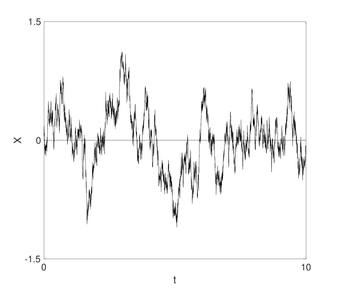
(a) $\beta=0.8$

(b) $\beta=2.0$

Figure 1: Simulation for infinite horizon Brownian bridges: $dX_{t}=-t^{\beta}X_{t}dt+dW_{t}$.

We take $\beta=0.8,2.0$ in Figure 1 by simulating the following SDE:

$$dX_{t}=-t^{\beta}X_{t}dt+dW_{t}\;.$$ (5.1)

The parameters are set as time step $h=0.01$, initial value $X_{0}=0$. It can be seen that when the index $\beta$ is larger, the rate of convergence to zero is faster.

We take $\beta=0.5,1.5$ in Figure 2 by simulating the SDE:

$$dX_{t}=-e^{\beta t}X_{t}dt+dW_{t},$$ (5.2)

The parameters are set as time step $h=0.005$, initial value $X_{0}=0$. The figure illustrates that when the index $\beta$ is larger, the rate of convergence to zero is faster.

Appendix A Proofs of Lemmas 2.1-2.3

Proof of Lemma 2.1. It is easy to see that both the denominator and the numerator go to infinity when $x\rightarrow\infty$. We can use the L’Hopital rule. The limit of the left hand side of (2.5) is the same as

$$\frac{g(x)\exp\left(\kappa\int_{0}^{x}g(u)du\right)}{\kappa g(x)\exp\left(\kappa\int_{0}^{x}g(u)du\right)}+\frac{1}{\kappa}\frac{g^{\prime}(x)}{g(x)}\frac{\int_{0}^{x}\exp\left(\kappa\int_{0}^{s}g(u)du\right)ds}{\exp\left(\kappa\int_{0}^{x}g(u)du\right)}\,.$$

The first summand is $1/\kappa$. Applying the L’Hopital rule to the last fraction of the second summand we see

$$\lim_{x\rightarrow\infty}\frac{\int_{0}^{x}\exp\left(\kappa\int_{0}^{s}g(u)du\right)ds}{\exp\left(\kappa\int_{0}^{x}g(u)du\right)}=\lim_{x\rightarrow\infty}\frac{\exp\left(\kappa\int_{0}^{x}g(u)du\right)}{\kappa g(x)\exp\left(\kappa\int_{0}^{x}g(u)du\right)}=0\,.$$

This implies $\lim_{x\rightarrow\infty}\frac{g(x)\int_{0}^{x}\exp\left(\kappa\int_{0}^{s}g(u)du\right)ds}{\exp\left(\kappa\int_{0}^{x}g(u)du\right)}=1/\kappa$. The lemma is then proved.

Proof of Lemma 2.2. Without loss of generality, we assume that $0<t_{1}<t_{2}<\infty$. Then

$$\sigma^{2}_{t_{1},t_{2}} =\mathbb{E}\left(\int_{0}^{t_{2}}\exp\left(-\int_{s}^{t_{2}}\alpha(u)du\right)dW_{s}-\int_{0}^{t_{1}}\exp\left(-\int_{s}^{t_{1}}\alpha(u)du\right)dW_{s}\right)^{2}$$

$$\leq 2\mathbb{E}\left[\int_{0}^{t_{1}}\left[\exp\left(-\int_{s}^{t_{2}}\alpha(u)du\right)-\exp\left(-\int_{s}^{t_{1}}\alpha(u)du\right)\right]dW_{s}\right]^{2}$$

$$+2\mathbb{E}\left(\int_{t_{1}}^{t_{2}}\exp\left(-\int_{s}^{t_{2}}\alpha(u)du\right)dW_{s}\right)^{2}$$

$$=2\int_{0}^{t_{1}}\left[\exp\left(-\int_{s}^{t_{2}}\alpha(u)du\right)-\exp\left(-\int_{s}^{t_{1}}\alpha(u)du\right)\right]^{2}ds$$

$$\qquad\qquad+2\int_{t_{1}}^{t_{2}}\exp\left(-2\int_{s}^{t_{2}}\alpha(u)du\right)ds=:I_{1}+I_{2}.$$ (A.1)

Denote

$$A_{*}(t)=\int_{0}^{t}\alpha(u)du\,,\quad t\geq 0\,.$$

We estimate the first term in (A) as follows. For any $0\leq\gamma\leq 1$, we have

$$I_{1} =2\left(1-\exp\left(-\int_{t_{1}}^{t_{2}}\alpha(u)du\right)\right)^{2}\int_{0}^{t_{1}}\exp\left(-2\int_{s}^{t_{1}}\alpha(u)du\right)ds$$

$$\leq C_{\gamma}\left(\int_{t_{1}}^{t_{2}}\alpha(u)du\right)^{2{\gamma}}\int_{0}^{t_{1}}\exp\left[-2A_{*}(t_{1})+2A_{*}(s)\right]ds$$

$$\leq C_{\gamma}\left(\int_{t_{1}}^{t_{2}}\alpha^{*}(u)du\right)^{2{\gamma}}\frac{\int_{0}^{t_{1}}\exp\left[2A_{*}(s)\right]ds}{\exp\left[2A_{*}(t_{1})\right]}$$

$$\leq C_{{\gamma}}\left(t_{2}-t_{1}\right)^{2{\gamma}}\left(\alpha^{*}(t_{2})\right)^{2{\gamma}}(\alpha(t_{1}))^{-1}\,,$$ (A.2)

where in the first inequality we have used the inequality that for any ${\gamma}\in[0,1]$, $1-e^{-x}\leq C_{\gamma}x^{\gamma}\,,x\geq 0$ for some constant $C_{\gamma}$, and the last inequality follows from Lemma 2.1. Now we estimate the second term in (A). Since $\alpha(t)$ is a positive function, we have

$$\int_{t_{1}}^{t_{2}}\exp\left(-2\int_{s}^{t_{2}}\alpha(u)du\right)ds\leq t_{2}-t_{1}\,.$$

On the other hand, we have

$$\int_{t_{1}}^{t_{2}}\exp\left(-2\int_{s}^{t_{2}}\alpha(u)du\right)ds \leq\int_{0}^{t_{2}}\exp\left(-2\int_{s}^{t_{2}}\alpha(u)du\right)ds\leq C(\alpha(t_{2}))^{-1}\,,$$

where in the above last inequality we use Lemma 2.1 again as in the above argument for $I_{1}$. Therefore,

$$\int_{t_{1}}^{t_{2}}\exp\left(-2\int_{s}^{t_{2}}\alpha(u)du\right)ds\leq C(t_{2}-t_{1})\wedge(\alpha(t_{2}))^{-1}\,.$$ (A.3)

Combining (A.2) and (A.3), for $0\leq{\gamma}\leq 1/2$, we have

$$\sigma^{2}_{t_{1},t_{2}} :=\mathbb{E}|X_{t_{2}}-X_{t_{1}}|^{2}\leq C_{{\gamma}}\left|t_{2}-t_{1}\right|^{2{\gamma}}\left(\alpha^{*}(t_{1}\vee t_{2})\right)^{2{\gamma}}(\alpha(t_{1}\wedge t_{2}))^{-1}$$

$$+C|t_{2}-t_{1}|\wedge(\alpha(t_{1}\vee t_{2}))^{-1}$$

$$\leq C_{{\gamma}}|t_{2}-t_{1}|^{2{\gamma}}\left[\left(\alpha^{*}(t_{1}\vee t_{2})\right)^{2{\gamma}}(\alpha(t_{1}\wedge t_{2}))^{-1}+(\alpha(t_{1}\vee t_{2}))^{-(1-2{\gamma})}\right]\,,$$

where we used the inequality

$$a\wedge b=(a\wedge b)^{\gamma}\cdot(a\wedge b)^{1-{\gamma}}\leq a^{\gamma}b^{1-{\gamma}},0\leq{\gamma}\leq 1\,.$$

Thus, we have proved the lemma.

Proof of Lemma 2.3. Let $m,n$ be integers, $m\geq 2$, $n\geq 1$. Since $X_{t_{2}}-X_{t_{1}}$ is a one-dimensional Gaussian process with mean zero and variance $\sigma^{2}_{t_{1},t_{2}}$ (defined by (2.6)) we can express its moments by this variance (see e.g. [14, Equation (3.1.8)])

$$\mathbb{E}|X_{t_{2}}-X_{t_{1}}|^{m}=\left\{\begin{array}[]{lcl}\frac{(2n)!(\sigma^{2}_{t_{1},t_{2}})^{n}}{2^{n}n!},&&\text{if }m=2n\text{ is even},\\ 0,&&{\text{if }m=2n+1\text{ is odd}}\,.\end{array}\right.$$ (A.4)

From now on we assume $m$ is an even integer. Denote

$$\rho(x;k):=C_{{\gamma}}x^{{\gamma}}k^{-\beta(1-2{\gamma})/2}\,.$$

From condition (i) in Theorem 2.1, we have $\alpha(t)\geq Ct^{\beta}$ for some $C>0$, which yields

$$\sigma_{t_{1},t_{2}}^{2} \leq C_{{\gamma}}|{t_{2}}-{t_{1}}|^{2{\gamma}}\left[\left(\alpha^{*}(k+1)\right)^{2{\gamma}}(\alpha(t_{1}\wedge t_{2}))^{-1}+(\alpha(t_{1}\vee t_{2}))^{-(1-2{\gamma})}\right]$$

$$\leq C_{{\gamma}}|{t_{2}}-{t_{1}}|^{2{\gamma}}\left[\left(\alpha^{*}(t_{1}\wedge t_{2}+1)\right)^{2{\gamma}}(\alpha(t_{1}\wedge t_{2}))^{-1}+(\alpha(t_{1}\wedge t_{2}))^{-(1-2{\gamma})}\right]$$

$$\leq C_{\gamma}|{t_{2}}-{t_{1}}|^{2{\gamma}}\left[C(t_{1}\wedge t_{2})^{-\beta}+C(t_{1}\wedge t_{2})^{-\beta(1-2{\gamma})}\right]$$

$$\leq C_{\gamma}|{t_{2}}-{t_{1}}|^{2{\gamma}}\left[Ck^{-\beta}+Ck^{-\beta(1-2{\gamma})}\right]$$

$$\leq\left(\rho(|t_{2}-t_{1}|;k)\right)^{2}\,.$$

Lemma 2.2 and (A.4) imply that

$$\mathbb{E}|X_{t_{2}}-X_{t_{1}}|^{m}\leq\frac{m!\sigma_{t_{1}t_{2}}^{m}}{2^{m/2}(m/2)!}\leq\frac{m!(\rho(|t_{2}-t_{1}|;k))^{m}}{2^{m/2}(m/2)!}\;.$$ (A.5)

Set

$$B_{k}:=\int_{k}^{k+1}\int_{k}^{k+1}\frac{|X_{t}-X_{s}|^{m}}{(\rho(|t-s|;k))^{m}}dsdt\,.$$ (A.6)

Then $B_{k}$ is finite. Take $\Psi(x)=x^{m}$. The inequality (A.5) implies

$$\mathbb{E}(B_{k})=\mathbb{E}\int_{k}^{k+1}\int_{k}^{k+1}\Psi\left(\frac{|X_{t}-X_{s}|}{\rho(|t-s|;k)}\right)dsdt\leq\frac{m!}{2^{m/2}(m/2)!}\;.$$ (A.7)

For any $N>1$, we have

$$\mathbb{E}\left(\sum_{k=1}^{\infty}\frac{B_{k}}{k^{N}}\right)=\sum_{k=1}^{\infty}\frac{\mathbb{E}(B_{k})}{k^{N}}<\infty.$$

This implies that

$$R_{N,m}:=\sum_{k=1}^{\infty}\frac{B_{k}}{k^{N}}~{}\textup{ is an almost surely finite random constant }\,.$$ (A.8)

Since all $B_{k}$ are positive, we see

$$B_{k}\leq R_{N,m}k^{N}~{}\textup{ for all positive number }N>1\textup{ and all integer }k\geq 1.$$ (A.9)

By virtue of the Garsia-Rodemich-Rumsey inequality, see e.g., Hu [14, Theorem 2.1], we can choose $m{\gamma}>2$, $2N/m<\beta$, and $2{\gamma}<1-2N/(\beta m)$ such that for any $t_{1},t_{2}\in[k,k+1]$

$$|X_{t_{2}}-X_{t_{1}}| \leq 8\int_{0}^{|t_{2}-t_{1}|}\Psi^{-1}\left(\frac{4B_{k}}{u^{2}}\right)\rho^{\prime}(u;k)du$$

$$=8\left(4B_{k}\right)^{1/m}{\gamma}C_{\gamma}k^{-\beta(1-2{\gamma})/2}\int_{0}^{|t_{2}-t_{1}|}u^{{\gamma}-1-\frac{2}{m}}du$$

$$\leq\frac{8\left(4R_{N,m}\right)^{1/m}{\gamma}}{{\gamma}-\frac{2}{m}}C_{\gamma}k^{-\beta\left[1-2{\gamma}-2N/(\beta m)\right]/2}$$

since $|t_{2}-t_{1}|\leq 1$, where $\Psi^{-1}(\cdot)$ is the inverse function of $\Psi(\cdot)$. This proves the lemma.

Appendix B Proof of Lemma 4.1

First let us recall a well-known result for Gaussian random variables. Let $Z_{1},\cdots,Z_{m}$ be a set of centered jointly Gaussian random variables with covariance matrix $F=\left(\mathbb{E}(Z_{i}Z_{j})\right)_{1\leq i,j\leq p}$. It is elementary from the well known form of the multivariate normal distribution that (cf. Berman [4]) the determinant of $F$ has the following representation:

$$\det(F)={\rm Var}(Z_{1}){\rm Var}(Z_{2}|Z_{1})\cdots{\rm Var}(Z_{p}|Z_{1},\cdots,Z_{p-1})\,,$$ (B.1)

where

$${\rm Var}(Z|Y_{1},\cdots,Y_{k}) = \mathbb{E}\left\{\left[Z-\mathbb{E}(Z|Y_{1},\cdots,Y_{k})\right]^{2}|Y_{1},\cdots,Y_{k})\right\}$$

$$= \mathbb{E}\left\{\left[Z-\mathbb{E}(Z|Y_{1},\cdots,Y_{k})\right]^{2}\right\}$$

denotes the conditional variance of $Z$ given $Y_{1},\cdots,Y_{k}$ and the above last identity follows from the fact that $Z-\mathbb{E}(Z|Y_{1},\cdots,Y_{k})$ is independent of $Y_{1},\cdots,Y_{k}$. For the solution of (1.2), we have

$${\rm Var}(X_{t}|X_{s}) = \mathbb{E}\left[(X_{t}-\mathbb{E}(X_{t}|X_{s}))^{2}\right]=\mathbb{E}\left[\left(\int_{s}^{t}e^{-\int_{r}^{t}\alpha(u)du}dW_{r}\right)^{2}\right]$$ (B.2)

$$= \int_{s}^{t}e^{-2\int_{r}^{t}\alpha(u)du}dr\geq(t-s)\exp\left(-2\alpha^{*}(t)(t-s)\right)\,.$$

For $u_{1}<u_{2}<\cdots<u_{p}$ applying the identity (B.1) to $X_{u_{1}}\,,\cdots,X_{u_{p}}$ and using the above inequality we have

$$\det(A) = \mathrm{Var}(X_{u_{1}}){\rm Var}(X_{u_{2}}|X_{u_{1}})\cdots{\rm Var}(X_{u_{p}}|X_{u_{1}},\cdots,X_{u_{p-1}})$$ (B.3)

$$\geq u_{1}(u_{2}-u_{1})\cdots(u_{p}-u_{p-1})\exp\left\{-2\alpha^{*}(u_{p})u_{p}\right\}\,.$$

This proves the first inequality in (4.2). On the other hand, by (B.2) we have for any $0\leq s<t<\infty$,

$${\rm Var}(X_{t}|{\cal F}_{s})\leq t-s\,.$$

This can be used to prove the second inequality in (4.2).

(a) $\beta=0.5$

(b) $\beta=1.5$

Figure 2: Simulation for infinite horizon Brownian bridges: $dX_{t}=-e^{\beta t}X_{t}dt+dW_{t}$.

References

- Avellaneda and Lipkin [2003] Avellaneda, M., Lipkin, M.D., 2003. A market-induced mechanism for stock pinning. Quant. Finance 3, 417–425. doi:10.1088/1469-7688/3/6/301.
- Ayache et al. [2008] Ayache, A., Wu, D., Xiao, Y., 2008. Joint continuity of the local times of fractional Brownian sheets. Ann. Inst. Henri Poincaré Probab. Stat. 44, 727–748. doi:10.1214/07-AIHP131.
- Back [1992] Back, K., 1992. Insider Trading in Continuous Time. Rev. Financ. Stud 5, 387–409. doi:10.1093/rfs/5.3.387.
- Berman [1973] Berman, S.M., 1973. Local nondeterminism and local times of Gaussian processes. Bull. Amer. Math. Soc. 79, 475–477. doi:10.1090/S0002-9904-1973-13225-2.
- Bertoin and Pitman [1994] Bertoin, J., Pitman, J., 1994. Path transformations connecting Brownian bridge, excursion and meander. Bull. Sci. Math. 118, 147–166.
- Bingham [1987] Bingham, N., 1987. Empirical processes with applications to statistics (wiley series in probability and mathematical statistics). Bull. London Math. Soc. 19, 298–300. doi:10.1112/blms/19.3.298.
- Brennan and Schwartz [1990] Brennan, M.J., Schwartz, E.S., 1990. Arbitrage in stock index futures. J. Bus. 63, S7–S31.
- Brigo and Mercurio [2006] Brigo, D., Mercurio, F., 2006. Interest rate models-theory and practice: with smile, inflation and credit. Springer Science & Business Media. doi:https://doi.org/10.1007/978-3-540-34604-3.
- Çetin and Danilova [2016] Çetin, U., Danilova, A., 2016. Markov bridges: SDE representation. Stochastic Process. Appl. 126, 651–679. doi:10.1016/j.spa.2015.09.015.
- Çetin and Danilova [2018] Çetin, U., Danilova, A., 2018. Dynamic Markov bridges and market microstructure. volume 90 of Probability Theory and Stochastic Modelling. Springer, New York. doi:10.1007/978-1-4939-8835-8. theory and applications.
- Ekström and Vaicenavicius [2020] Ekström, E., Vaicenavicius, J., 2020. Optimal stopping of a Brownian bridge with an unknown pinning point. Stochastic Process. Appl. 130, 806–823. doi:10.1016/j.spa.2019.03.018.
- Ekström and Wanntorp [2009] Ekström, E., Wanntorp, H., 2009. Optimal stopping of a Brownian bridge. J. Appl. Probab. 46, 170–180. doi:10.1239/jap/1238592123.
- Émery and Yor [2004] Émery, M., Yor, M., 2004. A parallel between Brownian bridges and gamma bridges. Publ. Res. Inst. Math. Sci. 40, 669–688. doi:10.2977/prims/1145475488.
- Hu [2017] Hu, Y., 2017. Analysis on Gaussian spaces. World Scientific Publishing Co. Pte. Ltd., Hackensack, NJ. doi:10.1142/10094.
- Hu et al. [2015] Hu, Y., Huang, J., Nualart, D., Tindel, S., 2015. Stochastic heat equations with general multiplicative Gaussian noises: Hölder continuity and intermittency. Electron. J. Probab. 20, no. 55, 50. doi:10.1214/EJP.v20-3316.
- Hull and White [2015] Hull, J., White, A., 2015. Pricing Interest-Rate-Derivative Securities. Rev. Financ. Stud 3, 573–592. doi:10.1093/rfs/3.4.573.
- Karatzas and Shreve [1991] Karatzas, I., Shreve, S.E., 1991. Brownian motion and stochastic calculus. volume 113 of Graduate Texts in Mathematics. Second ed., Springer-Verlag, New York. doi:10.1007/978-1-4612-0949-2.
- Kôno [1977] Kôno, N., 1977. Hölder conditions for the local times of certain Gaussian processes with stationary increments. Proc. Japan Acad. Ser. A Math. Sci. 53, 84–87. doi:10.3792/pjaa.53.84.
- Kyle [1985] Kyle, A.S., 1985. Continuous auctions and insider trading. Econometrica 53, 1315–1335. doi:10.2307/1913210.
- Marcus and Rosen [2006] Marcus, M.B., Rosen, J., 2006. Markov processes, Gaussian processes, and local times. volume 100 of Cambridge Studies in Advanced Mathematics. Cambridge University Press, Cambridge. doi:10.1017/CBO9780511617997.
- Pitman [1999] Pitman, J., 1999. The distribution of local times of a Brownian bridge, in: Séminaire de Probabilités, XXXIII. Springer, Berlin. volume 1709 of Lecture Notes in Math., pp. 388–394. doi:10.1007/BFb0096528.
- Pitman and Yor [1982] Pitman, J., Yor, M., 1982. A decomposition of Bessel bridges. Z. Wahrsch. Verw. Gebiete 59, 425–457. doi:10.1007/BF00532802.
- Revuz and Yor [1999] Revuz, D., Yor, M., 1999. Continuous martingales and Brownian motion. volume 293 of Grundlehren der Mathematischen Wissenschaften [Fundamental Principles of Mathematical Sciences]. Third ed., Springer-Verlag, Berlin. doi:10.1007/978-3-662-06400-9.
- Shepp [1969] Shepp, L.A., 1969. Explicit solutions to some problems of optimal stopping. Ann. Math. Statist. 40, 993–1010. doi:10.1214/aoms/1177697604.