K2-280 b - a low density warm sub-Saturn around a mildly evolved star

Abstract

We present an independent discovery and detailed characterisation of K2-280 b, a transiting low density warm sub-Saturn in a 19.9-day moderately eccentric orbit ($e$ = $0.35_{-0.04}^{+0.05}$  ) from K2 campaign 7. A joint analysis of high precision HARPS, HARPS-N, and FIES radial velocity measurements and K2 photometric data indicates that K2-280 b has a radius of $R_{\mathrm{b}}$ = $7.50\pm 0.44$ $R_{\oplus}$ and a mass of $M_{\mathrm{b}}$ = $37.1\pm 5.6$ $M_{\oplus}$, yielding a mean density of $\rho_{\mathrm{b}}$ = $0.48_{-0.10}^{+0.13}$ ${\rm g\,cm^{-3}}$. The host star is a mildly evolved G7 star with an effective temperature of $T_{\mathrm{eff}}$ =  $5500\pm 100$ $\mathrm{K}$ , a surface gravity of $\log\,g_{\star}$ = 4.21 $\pm$ 0.05 (cgs), and an iron abundance of $\mathrm{[Fe/H]}$ = ${0.33}\,{\pm}\,{0.08}$ $\mathrm{dex}$, and with an inferred mass of $M_{\star}$ =  $1.03\pm 0.03$ $M_{\odot}$ and a radius of $R_{\star}$ =  $1.28\pm 0.07$ $R_{\odot}$. We discuss the importance of K2-280 b for testing formation scenarios of sub-Saturn planets and the current sample of this intriguing group of planets that are absent in the Solar System.

1 Introduction

The main advantage of the extended NASA’s Kepler mission (Borucki et al., 2010), known as K2 (Howell et al., 2014), was a much larger number of bright stars in its fields of view located along the ecliptic. A significant number of planets transiting bright stars have been discovered in all K2 campaigns (e.g., Montet et al., 2015; Crossfield et al., 2016; Vanderburg et al., 2016; Dressing et al., 2017; Petigura et al., 2018; Mayo et al., 2018; Yu et al., 2018a; Crossfield et al., 2018; Livingston et al., 2018). Some of these planets were only validated, but many were characterized by means of high precision radial velocity (RV) measurements that enabled mass determination with precision better than 20% (e.g., Vanderburg et al., 2015; Gandolfi et al., 2017; Christiansen et al., 2017; Prieto-Arranz et al., 2018; Rodriguez et al., 2018; Barragán et al., 2018b; Malavolta et al., 2018). However much higher precision is needed to distinguish between various possible planetary compositions (see e.g. Dorn et al., 2015, and references therein). Mass determination with such precision for small planets ($R_{\mathrm{p}}$ = 1–4 $\mathrm{R_{\oplus}}$) were possible only for short period ($P_{\mathrm{orb}}$ $\lesssim$ 10 days) sub-Neptunes and super-Earths, which induces RV semi-amplitudes on the parent stars of a few $\mathrm{m\,s^{-1}}$, and for stars hosting ultra-short period planets, for which the Doppler reflex motion is enhanced by the extremely short orbital period ($P_{\mathrm{orb}}$ $<$ 1 day; Winn et al., 2018, and references therein). Most of the small K2 planets with precise mass determination orbit bright stars, i.e., stars brighter than $V$ = 11.5, which is the current limit for $\sim$1 $\mathrm{m\,s^{-1}}$ precision with spectrographs mounted at 3–4-m class telescopes (Pepe et al., 2013). The constraints for precise determination of planetary masses are naturally more relaxed for higher-mass planets, enabling us to study super-Neptune/sub-Saturn planets ($R_{\mathrm{p}}$ = 4–8 $\mathrm{R_{\oplus}}$) with longer orbital periods around fainter stars.

Sub-Saturns form a very intriguing group of planets that have no counterpart in the Solar System. Their main characteristic is a significant contribution of both heavy metal cores and low density gaseous envelopes to the total planet mass (Petigura et al., 2016). They are thus important laboratories to study envelope accretion. As shown by Petigura et al. (2017), the population of sub-Saturns has a very uniform distribution of the planetary mass between $\sim$6 and 60 $\mathrm{M_{\oplus}}$. Similar to gas-giant planets, they are also found to orbit mainly metal-rich stars. Finally, the most massive sub-Saturns are often the only detected planet in the system and orbit their parent stars on eccentric orbits, which suggests that dynamical instability might have played an important role in their formation.

Here we present an independent discovery and characterisation of a low mass, sub-Saturn planet on a 20-d orbit around a relatively faint ($V$ = 12.5), metal rich ($\mathrm{[Fe/H]}$ = ${0.33}\,{\pm}\,{0.08}$ $\mathrm{dex}$), slightly evolved K2 star that was proposed as a planet candidate by Petigura et al. (2018) and Mayo et al. (2018), and statistically validated as a planet by Livingston et al. (2018). This kind of planets was usually avoided by RV follow-up of K2 candidates because of the faintness of their host stars. Besides, slightly evolved stars are typically avoided in RV follow-up projects, because of their higher expected stellar jitter (see e.g. Hekker et al., 2006; Hekker et al., 2008; Tayar et al., 2019, and references therein). Both these effects may bias the statistical analysis of warm-giant planets. K2-280 b joins a sample of 30 sub-Saturns with mean densities determined with precision better than 50% discovered mainly by Kepler and K2 (see Petigura et al., 2017, and references therein for first 23 planets).

This work was done as a part of the KESPRINT collaboration, which aims to confirm and characterise K2 and TESS planets. In Section 2 we describe the observations of K2-280, specifically the K2 photometry, the NOT/FIES, ESO/HARPS, and TNG/HARPS-N high-resolution spectroscopy follow-up, and the high-contrast imaging. In Section 3 and 4 we present the properties of the host star K2-280 and the global analysis of photometric and Doppler data, respectively. In Section 5 we finally summarise and discuss the characteristics of K2-280 b in the context of the properties of the known population of sub-Saturn planets with mean densities determined with precision better than 50%.

2 Observations and data reductions

2.1 K2 Photometry

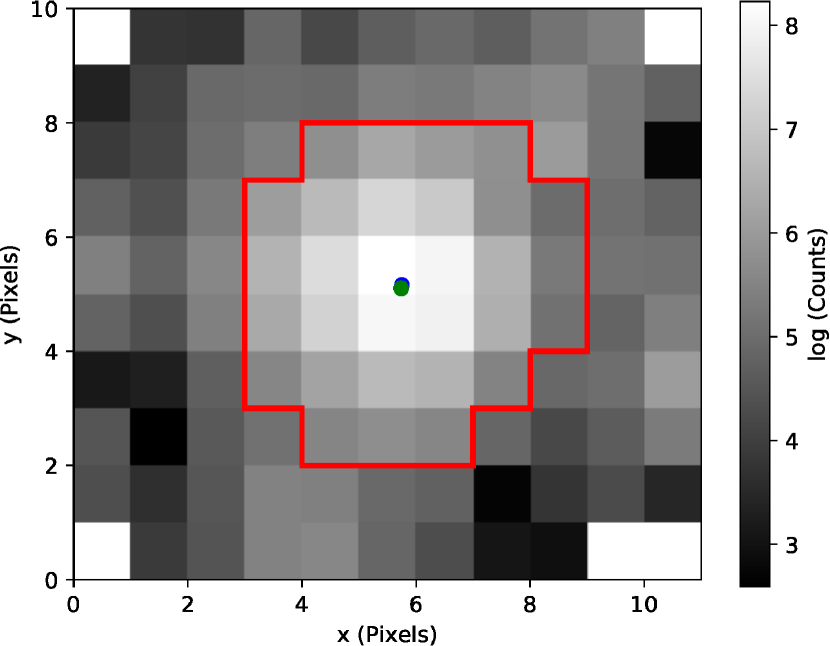
Figure 1: K2 image of K2-280. Red lines shows the aperture defined by the amount of light of each pixel and level of background light. The electron count is indicates by the intensity of shading (light grey for high and dark grey for low count). The green circle indicates the current position of the target in the EPIC catalog, and the blue circle is the centre of the flux distribution. The scale of the image is the Kepler pixel scale of 3.98 arcsec/pix. The K2 image is not a rectangle, but it is irregularly shaped. The white pixels in the corners contain no data.

K2-280 was one of 13 469 long cadence targets observed from October 4^th to December 26^th 2015 (UT) during K2 campaign 7. It was proposed as a target by GO programmes 7030 (PI Howard), and 7085 (PI Burke). We downloaded K2-280 images from the MAST archive and used them to produce a de-trended K2 light curve as described in detail in Dai et al. (2017). Figure 1 shows the pixel mask used to perform simple aperture photometry. We used the box fitting least-square (BLS) routine (Kovács et al., 2002; Jenkins et al., 2010), improved by implementation of the optimal frequency sampling described in Ofir (2014) to search for transiting planet candidates in all Field 7 targets light curves. We detected transits of K2-280 b with a signal-to-noise ratio (SNR) of 24.5, depth of $\sim$3.5 $\times 10^{-3}$, period of $P\,=\,19.89518\,\pm\,0.00028$ days, and a mid-time of the first transit $T_{0}\,=\,2457307.58101\,\pm\,0.00059$ days in Barycentric Julian Date in the Barycentric Dynamical Time (BJD_TDB; see, e.g., Eastman et al., 2010). The de-trended light curve of K2-280 with the correction for baseline flux variations and centroid motions is presented in Figure 2 with the 4 transits observed by K2 highlighted with red lines. We removed the baseline flux variation by fitting a spline function with a width of 3 days. In Table 1 we report the main identifiers of K2-280, along with its equatorial coordinates, space motion, distance, and optical and near-infrared magnitudes.

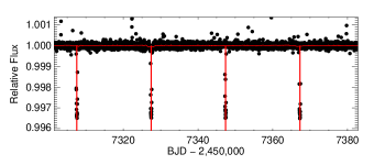
Figure 2: Detrended K2 light curve of K2-280. The 4 transits observed by K2 are marked by vertical solid red lines. The horizontal red line is the local median flux level with a window of 0.5-day.

Table 1: Properties of K2-280.

Parameter	Value	Source
Coordinates and Main Identifiers
RA 2000.0 (hours)	19:26:22.881	Gaia DR2
Dec 2000.0 (deg)	-22:14:51.552	Gaia DR2
Gaia DR2 Identifier	6772454416893148928	Gaia DR2
2MASS Identifier	19262288-2214514	2MASS PSC
UCAC Identifier	339-184113	UCAC4
EPIC Identifier	216494238	EPIC
TIC Identifier	119605900	TIC
Optical and Near-Infrared Magnitudes
$K_{p}$ (mag)	12.302	K2 EPIC
$B$ (mag)	13.269 $\pm$ 0.010	UCAC4
$V$ (mag)	12.536 $\pm$ 0.040	UCAC4
$R$ (mag)	12.41 $\pm$ 0.07	UCAC4
$G$ (mag)	12.3604 $\pm$ 0.0002	Gaia DR2
$g$ (mag)	12.850 $\pm$ 0.020	UCAC4
$r$ (mag)	12.320 $\pm$ 0.020	UCAC4
$i$ (mag)	12.067 $\pm$ 0.040	UCAC4
$J$ (mag)	11.141 $\pm$ 0.021	2MASS
$H$ (mag)	10.854 $\pm$ 0.024	2MASS
$K$ (mag)	10.765 $\pm$ 0.019	2MASS
Space Motion and Distance
$\mathrm{PM_{\mathrm{RA}}}$ ($\mathrm{mas\,yr^{-1}}$)	4.44 $\pm$ 0.08	Gaia DR2
$\mathrm{PM_{\mathrm{DEC}}}$ ($\mathrm{mas\,yr^{-1}}$)	-12.50 $\pm$ 0.07	Gaia DR2
RVγ,HARPS ($\mathrm{km\,s^{-1}}$)	$-1.1934_{-0.0011}^{+0.0011}$	This work
RVγ,HARPS-N ($\mathrm{km\,s^{-1}}$)	$-1.1907_{-0.0011}^{+0.0011}$	This work
RVγ,FIES ($\mathrm{km\,s^{-1}}$)	$-1.2349_{-0.0039}^{+0.0038}$	This work
$\pi_{\star}$(mas)	${2.526}\,{\pm}\,{0.111}$	Gaia DR2
$d_{\star}$(pc)	$391.5^{+7.5}_{-7.2}$	Bailer-Jones et al. (2018)
$U$ ($\mathrm{km\,s^{-1}}$)	-7.78 $\pm$ 0.06	This work
$V$ ($\mathrm{km\,s^{-1}}$)	-5.98 $\pm$ 0.84	This work
$W$ ($\mathrm{km\,s^{-1}}$)	-9.18 $\pm$ 0.71	This work
Photospheric Parameters
$T_{\mathrm{eff}}$ (K)	5500 $\pm$ 100	This work
$\log\,g_{\star}$(a) (dex)	4.00 $\pm$ 0.10	This work
$\log\,g_{\star}$(b) (dex)	4.21 $\pm$ 0.05	This work
$\mathrm{[Fe/H]}$ (dex)	0.33 $\pm$ 0.08	This work
Derived Physical Parameters
$M_{\star}$ ($\mathrm{M_{\odot}}$)	$1.03\pm 0.03$	This work
$R_{\star}$ ($\mathrm{R_{\odot}}$)	$1.28\pm 0.07$	This work
$\rho_{\star}$ ($\mathrm{g\,cm^{-3}}$)	$0.8_{-0.13}^{+0.16}$	This work
Age (Gyr)	8.96 $\pm$ 1.70	This work
Stellar Rotation
$\mathit{v}_{\mathrm{rot}}\sin\,i_{\star}$ ($\mathrm{km\,s^{-1}}$)	3.0 $\pm$ 1.0	This work

Notes – ^(a) From spectroscopy. ^(b) From stellar mass and radius.

2.2 High-dispersion spectroscopy

High-dispersion spectroscopic observations of K2-280 were obtained between April 30^th 2016 (UT) and May 7^th 2019 (UT) using ESO/HARPS, TNG/HARPS-N, and NOT/FIES spectrographs. We collected a total of 18 HARPS, 14 HARPS-N and 6 FIES spectra. The details of these observations are given in the subsections below. Table 2 gives the time stamps of the spectra in BJD_TDB, the RVs along with their $1\sigma$ error bars, as well as the bisector inverse slope (BIS) and full-width at half maximum (FHWM) of the cross-correlation function (CCF).

2.2.1 ESO/HARPS

We started the RV follow-up of K2-280 using the High Accuracy Radial velocity Planet Searcher (HARPS) spectrograph (Mayor et al., 2003, R$\approx$115 000) mounted at the ESO 3.57-m telescope of La Silla Observatory in Chile. We acquired 18 spectra between April 30^th 2016 (UT) and April 27^th 2018 (UT) under the observing programmes 097.C-0571(B), 097.C-0948(A), 098.C-0860(A), 099.C-0491(A), 0101.C-0407(A), and 60.A-9700(G), setting the exposure times to 1200–3600 seconds. The dedicated on-line HARPS Data Reduction Software (DRS) was used to reduce the spectra, and extract the Doppler measurements and spectral activity indicators. The SNR per pixel at 5500 Å is in the range 22–46. Radial velocities were measured by cross-correlating the extracted spectra with a G2 numerical mask (Baranne et al., 1996). The uncertainties of the measured RVs are in the range 2.1–8.1 $\mathrm{m\,s^{-1}}$ with a mean value of 4.2 $\mathrm{m\,s^{-1}}$.

2.2.2 TNG/HARPS-N

Between July 16^th 2016 (UT) and May 7^th 2019 (UT) we collected 14 spectra with the HARPS-N spectrograph (Cosentino et al., 2012, R$\approx$115 000) mounted at the 3.58-m Telescopio Nazionale Galileo (TNG) of Roque de los Muchachos Observatory in La Palma, Spain, under the observing programmes A33TAC_15, OPT17A_64, CAT17A_91, and CAT19A_97. The exposure time was set to 1200–3600, based on weather conditions and scheduling constraints, leading to a SNR per pixel of 15–47 at 5500 Å. The spectra were extracted using the off-line version of the HARPS-N DRS pipeline. Doppler measurements and spectral activity indicators were measured using an on-line version of the DRS, the YABI tool, by cross-correlating the extracted spectra with a G2 mask (Baranne et al., 1996). The uncertainty of the measured RVs are in the range 2.0–8.6 $\mathrm{m\,s^{-1}}$, with a mean value of 4.5 $\mathrm{m\,s^{-1}}$.

2.2.3 NOT/FIES

We acquired 6 additional spectra using the FIbre-fed Échelle Spectrograph (FIES; Frandsen & Lindberg, 1999; Telting et al., 2014) mounted at the 2.56-m Nordic Optical Telescope (NOT) of Roque de los Muchachos Observatory (La Palma, Spain). The observations were carried out between June 26^th and September 6^th 2016 (UT), as part of the OPTICON observing programme 53-109. We used the FIES high-resolution mode, which provides a resolving power of $R$ = 67 000 in the spectral range 3700–7300 Å. Following the observing strategy described in Buchhave et al. (2010) and Gandolfi et al. (2015), we traced the RV drift of the instrument by acquiring long-exposed ThAr spectra ($T_{\mathrm{exp}}$ $\approx$ 35 sec) immediately before and after each science exposure. The exposure time was set to 2700–3600 seconds, according to the sky conditions and scheduling constraints. The data reduction follows standard IRAF and IDL routines, which includes bias subtraction, flat fielding, order tracing and extraction, and wavelength calibration. Radial velocity measurements were computed via multi-order cross-correlations with the RV standard star HD 50692 (Udry et al., 1999), observed with the same instrument set-up as K2-280. The SNR per pixel at 5500 Å of the extracted spectra is in the range 15–35. The uncertainties are in the range 6.8–13.6 $\mathrm{m\,s^{-1}}$ with a mean value of 9.7 $\mathrm{m\,s^{-1}}$.

Table 2: HARPS, HARPS-N, and FIES radial velocities (RVs), bisector inverse slope (BIS), and full-width at half maximum (FWHM) of the cross-correlation function.

BJDTDB	RV	$\sigma_{\mathrm{RV}}$	BIS	$\sigma_{\mathrm{BIS}}$	$\mathrm{FWHM}$
-$2\,450\,000$	($\mathrm{m\,s^{-1}}$)	($\mathrm{m\,s^{-1}}$)	($\mathrm{m\,s^{-1}}$)	($\mathrm{m\,s^{-1}}$)	($\mathrm{km\,s^{-1}}$)
FIES
7566.606106	-1236.447	10.145	-25.604	8.240	12.240
7570.575852	-1248.492	8.236	-19.745	5.424	12.237
7579.594362	-1221.025	13.568	-15.325	10.160	12.257
7583.604507	-1227.357	11.149	-1.138	9.710	12.232
7600.515019	-1233.204	8.028	-36.207	7.614	12.283
7638.387601	-1225.100	6.816	-23.315	4.940	12.220
HARPS-N
7585.595242	-1192.158	6.794	-15.933	9.608	7.354
7603.514891	-1191.265	5.126	-13.175	7.249	7.363
7611.572851	-1201.759	8.653	-15.272	12.238	7.371
7892.699273	-1195.302	3.475	-5.393	4.915	7.348
7921.702566	-1191.619	3.014	-7.642	4.263	7.359
7958.534636	-1194.254	7.553	-39.517	10.682	7.360
7965.540153	-1197.765	2.357	-14.982	3.334	7.360
8013.363503	-1186.028	1.991	-18.747	2.816	7.366
8013.404784	-1185.686	2.117	-30.544	2.994	7.362
8014.362082	-1185.942	2.722	-28.539	3.850	7.352
8014.402379	-1189.116	2.756	-24.429	3.898	7.365
8015.359376	-1178.088	5.620	-11.056	7.948	7.349
8015.402150	-1187.664	5.605	-13.530	7.927	7.368
8610.724187	-1193.898	4.651	-17.515	6.577	7.359
HARPS
7508.854151	-1195.313	3.185	-5.317	4.504	7.447
7511.892058	-1194.114	4.462	-2.236	6.310	7.409
7609.625616	-1195.440	2.732	19.011	3.865	7.415
7619.566531	-1184.749	4.551	16.474	6.437	7.413
7637.587335	-1181.617	6.366	-13.161	9.004	7.400
7638.596015	-1172.262	7.600	-21.324	10.748	7.447
7639.571271	-1181.987	6.990	-34.526	9.885	7.389
7645.538147	-1194.348	4.671	11.465	6.607	7.433
7682.520265	-1194.190	5.191	17.641	7.342	7.420
7984.617196	-1190.758	2.370	-5.857	3.352	7.422
7986.590931	-1203.107	3.223	-1.852	4.559	7.421
7987.587443	-1197.553	2.285	13.255	3.232	7.415
7990.553698	-1195.977	2.729	24.528	3.859	7.418
7990.593359	-1207.601	2.817	-20.535	3.983	7.396
7992.576732	-1189.811	2.093	16.287	2.950	7.419
7992.609762	-1187.701	2.759	-9.069	3.902	7.408
8003.594697	-1191.639	3.620	-0.841	5.110	7.401
8235.876739	-1189.777	8.100	-22.636	11.455	7.409

2.3 High contrast imaging

To search for nearby stars and estimate a potential contamination factor from such sources we used a high contrast image of K2-280 publicly available on the ExoFOP-K2 website. The image was acquired on June 19^th 2016 (UT) using the Frederick C. Gillett Gemini North telescope and its adaptive optics (AO) system facility, ALTAIR with a natural guide star along with a Near InfraRed Imager and spectrograph (NIRI) (Hodapp et al., 2003) using the Brackett Gamma (Br$\gamma$) filter (Gemini-North ID G0218) centered at 2.17 $\mathrm{\mu m}$, under Gemini Science Program GN-2016A-LP-5. Two faint stars are visible on the Gemini-North/NIRI+ALTAIR AO image of K2-280 (Figure 3): a very close-in companion at $\sim$0.4″ west–north-west (W–NW), and a distant source at $\sim$6.6″south–south-east (S–SE) of K2-280. We carefully analyzed the Gemini-North/NIRI+ALTAIR AO image of K2-280. Table 3 reports separations, position angles, the magnitude difference $\Delta m_{Br\gamma}$, and the $\Delta F_{Br\gamma}$ flux-ratio of these two objects relative to K2-280. Their brightness ratio at 2.17 $\mathrm{\mu m}$ is comparable to the observed K2 transit depth (3500 ppm), which requires their consideration as sources of false positives (see Section 3.5).

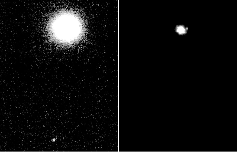
Figure 3: AO image of the surroundings of K2-280 obtained with the Gemini-North/NIRI+ALTAIR instrument. Both panels show the same image, with a FOV of 8.7″ in the N-S and 6.7″ in the E-W direction (north to the top and east to the left), but with different brightness scales. The left panel shows the star at 6.6″ in the S–SE direction and the right one the close neighbor at 0.4″ W–NW of K2-280.

3 Properties of the host star

3.1 Gaia measurements

K2-280 is among a small sub-sample of ESA’s Gaia mission (Gaia Collaboration et al., 2016) targets for which the Gaia DR2 (Gaia Collaboration et al., 2018) – a first Gaia-only catalogue – provides not only astrometric measurements, but also astrophysical parameters (radii, luminosities, extinctions, and reddening) and median radial velocities. Gaia DR2 astrometric parameters of K2-280 are included in Table 1. Gaia DR2 values of stellar radius and median RV of K2-280 agree with the values determined in the subsections below.

3.2 Photospheric parameters and stellar rotation velocity measurements using SME

We followed the procedure described in Fridlund et al. (2017) and Persson et al. (2018) and analysed the co-added spectra from HARPS, HARPS-N, and FIES with the spectral analysis package Spectroscopy Made Easy (SME; Valenti & Piskunov, 1996; Valenti & Fischer, 2005; Piskunov & Valenti, 2017) to derive the effective temperature $T_{\mathrm{eff}}$, surface gravity $\log\,g_{\star}$, iron abundance [Fe/H], and projected rotational velocity $\mathit{v}_{\mathrm{rot}}\sin\,i_{\star}$. Spectroscopy Made Easy uses grids of atmosphere models to calculate synthetic stellar spectra, which are fitted to the observed spectra using a $\chi^{2}$-minimising procedure. We use the line wings of H_α, which is rather insensitive to $\log\,g_{\star}$ for this spectral type, to model $T_{\mathrm{eff}}$ (with a fixed $\log\,g_{\star}$), and the line wings of the Ca i triplet to model $\log\,g_{\star}$ (with a fixed $T_{\mathrm{eff}}$). We used the latest version of the software (5.2.2) and line lists from the Vienna atomic line database. The model spectra were taken from ATLAS12 (Kurucz, 2013). The calibration equations for Sun-like stars from Bruntt et al. (2010) and Doyle et al. (2014) were adopted to fix the micro- and macroturbulent velocities, $\mathit{v}_{\mathrm{mic}}$ and $\mathit{v}_{\mathrm{mac}}$ to 0.5 and 1.0 $\mathrm{km\,s^{-1}}$, respectively. The spectroscopic parameters derived from the HARPS, HARPS-N, and FIES co-added spectra agree well within their nominal error bars. The final adopted values are $T_{\mathrm{eff}}$ = 5500 $\pm$ 100 K, $\log\,g_{\star}$ = 4.00 $\pm$ 0.10 (cgs), and [Fe/H] = 0.33 $\pm$ 0.08 dex (Table 1). They are defined as the weighted mean of the individual parameters derived from the HARPS, HARPS-N, and FIES co-added spectra.

3.3 Photospheric parameters and radius measurements using SpecMatch-emp

As a sanity check, we also analysed the co-added HARPS and HARPS-N spectra using the SpecMatch-emp software package (Yee et al., 2017). SpecMatch-emp estimates the stellar effective temperature $T_{\mathrm{eff}}$, radius $R_{\star}$, and iron abundance $\mathrm{[Fe/H]}$ by fitting the spectral region between 5000 and 5900 Å to hundreds of library spectra gathered by the California Planet Search programme. Following the procedure described in Hirano et al. (2018), we reformatted the co-added HARPS and HARPS-N spectra so that they can be read by SpecMatch-emp. We found $T_{\mathrm{eff}}$ = 5597 $\pm\,$110 K and $\mathrm{[Fe/H]}$ = 0.33 $\pm$ 0.08 dex, which agree with the effective temperature and iron abundance determined with SME (Table 1) within 1$\sigma$. We found also that K2-280 is a slightly evolved star with a stellar radius of $R_{\star}$ = 1.33 $\pm$ 0.21 $\mathrm{R_{\oplus}}$. We finally obtained a first estimate of the stellar mass ($M_{\star}$ = 1.16 $\pm$ 0.08$~{}\mathrm{M_{\oplus}}$) via Monte Carlo simulations using the empirical equations by Torres et al. (2010) alongside $T_{\mathrm{eff}}$, $\mathrm{[Fe/H]}$, and $R_{\star}$.

Table 3: Relative properties of the two nearby stars to K2-280 detected with the Gemini-North/NIRI+ALTAIR.

Parameter	W–NW	S–SE
	close-in star	distant star
Separation (″)	$0.38\pm 0.011$	$6.598\pm 0.011$
Position Angle (deg)	$286.2\pm 1.5$	$173.3\pm 1.5$
$\Delta m_{Br\gamma}$ (mag)	$4.72\pm 0.15$	$6.65\pm 0.15$
$\Delta F_{Br\gamma}$ relative flux	$(1.3\pm 0.2)\times 10^{-2}$	$(2.2\pm 0.4)\times 10^{-3}$

3.4 Physical parameters

We refined the fundamental parameters of K2-280 utilising the web interface PARAM 1.3 along with PARSEC isochrones (Bressan et al., 2012). Following the method described in Gandolfi et al. (2008), we found that the interstellar extinction along the line of sight to the star is $A_{\mathrm{v}}\,=\,0.10\,\pm\,0.05$. Using the effective temperature and iron abundance derived in Section 3.2, alongside the extinction-corrected visual magnitude and the Gaia parallax (Table 1), we determined a mass of $M_{\star}$ = 1.03 $\pm$ 0.03 $\mathrm{M_{\odot}}$ and a radius of $R_{\star}$ = 1.28 $\pm$ 0.07 $\mathrm{R_{\odot}}$, which agree with the values derived in Section 3.3. Stellar mass and radius implies a surface gravity of $\log\,g_{\star}$ = 4.21 $\pm$ 0.05 (cgs), which is higher than our spectroscopic value of $4.0\,\pm\,0.1$ (cgs), but within its 2$\sigma$ error bars. The age of the star was constrained to be 8.9 $\pm$ 1.7 Gyr, further confirming the evolved status of K2-280. The values of stellar radius and mass agree within 3-$\sigma$ with the ones determined by Petigura et al. (2018) ($R_{\star}=1.45_{-0.18}^{+0.20}$ $\mathrm{R_{\odot}}$, $M_{\star}=1.17_{-0.08}^{+0.10}$ $\mathrm{M_{\odot}}$), Mayo et al. (2018) ($R_{\star}=1.064_{-0.047}^{+0.069}$ $\mathrm{R_{\odot}}$, $M_{\star}=1.101_{-0.028}^{+0.025}$ $\mathrm{M_{\odot}}$), and Livingston et al. (2018) ($R_{\star}=1.28\pm 0.03$ $\mathrm{R_{\odot}}$, $M_{\star}=1.11\pm 0.04$ $\mathrm{M_{\odot}}$). We stress that the parameter estimates determined in the three works listed above are based on spectra with relatively low SNR, in contrast to our co-added, high SNR, HARPS, HARPS-N and FIES spectra. Petigura et al. (2018) and Livingston et al. (2018) used the same spectra collected with the HIgh Resolution Echelle Spectrometer (HIRES Vogt et al., 1994) mounted on 10-m Keck I telescope, with typical SNR = 45 for stars with $V<13.0$. Mayo et al. (2018) used spectra collected with Tillinghast Reflector Echelle Spectrograph (TRES) mounted on the 1.5-m Tillinghast telescope at the Whipple Observatory on Mt. Hopkins in Arizona with even lower SNR.

We also calculated the $UVW$ space velocities of K2-280 using the IDL code gal_uvw (based upon Johnson & Soderblom, 1987), using the Gaia DR2 proper motions and parallax, and the average of the HARPS and HARPS-N systemic velocities $\gamma$ (Table 1). Our calculated values of $UVW$ are listed in Table 1; we quote values in the local standard of rest using the solar motion of Coşkunoǧlu et al. (2011). We then used the methodology of Reddy et al. (2006) to determine the Galactic population membership of K2-280. We found that K2-280 has a $>99\%$ probability of belonging to the Galactic thin disk, and less than $1\%$ of belonging to either the thick disk or the halo. This is consistent with K2-280’s high metallicity of $\mathrm{[Fe/H]}$ = ${0.33}\,{\pm}\,{0.08}$ $\mathrm{dex}$.

The final adopted stellar parameters are listed in Table 1. The effective temperature and surface gravity translate into a G7 V spectral type (Gray & Corbally, 2009).

3.5 Faint AO companions

From the two faint companions to K2-280 identified in the Gemini-North/NIRI+ALTAIR AO image (Section 2.3), the one located 6.6″ S–SE of K2-280 was identified in the Gaia DR2 as the source 6772454206445987712. Based on its very small proper motion ($\mathrm{PM_{RA}}$ = 0.29 $\pm$ 0.52$\,\mathrm{mas\,yr^{-1}}$ and $\mathrm{PM_{DEC}}$ = $-$0.92 $\pm$ 0.45$\,\mathrm{mas\,yr^{-1}}$) and distance found by Bailer-Jones et al. (2018) ($d=5.103^{+3.435}_{-2.094}$ kpc), we concluded that it is a background star. Using the Gaia G-band magnitude ($G\,=\,18.765\pm 0.010$), we derived a G-band brightness ratio relative to K2-280 of 0.0027 $\pm$ 0.0001. Considering the close similarity between the Gaia G-band and the Kepler passband, this companion is too faint to be the source of the transit signal detected in the K2 data.

For the close-in W–NW companion we cannot determine whether it is physically bound or unbound to K2-280. Yet, its very small angular separation of 0.4″ supports the binary scenario for K2-280. Based on the Besançon Galactic population model (Robin et al., 2003) and following the procedure described in Hjorth et al. (2019) we calculated the probability of a chance alignment to be $0.04\%$. Assuming that the W–NW companion is physically bound to K2-280, we can then obtain further information about it.

The central wavelength of 2.19 $\mathrm{\mu m}$ of the Br$\gamma$ filter is nearly identical to that of the near-infrared $K$ band. Therefore we used the apparent $K$ magnitude of K2-280 from Table 1 ($m_{K}=10.765\pm 0.019$) and the magnitude difference from Table 3 to calculate absolute $K$ magnitudes of both stars. They are equal to $M_{K}=2.778\pm 0.090$ for K2-280 and $M_{K}=7.50\pm 0.22$ for the nearby companion. Making use of the Dartmouth isochrone table (Dotter et al., 2008) for metallicity $\mathrm{[Fe/H]}=0.36$ and ages between 9 and 11 Gyr, we estimated that the nearby companion is a M3.5–M4 red-dwarf with a mass between 0.21 and 0.28 $\mathrm{M_{\odot}}$. Using its angular separation from Table 3 and the DR2 parallax of K2-280  we calculated a lateral separation from K2-280 of $150.4^{+8.2}_{-7.7}$ au. We note that current models of planetary formations in wide binary stellar systems predict a shortage of giant planets in binaries with separations of $\leq$100 au (e.g., Nelson, 2000; Mayer et al., 2005; Thébault et al., 2006); the nearby companion should therefore not have affected the formation of the K2-280 planetary system.

Based on the Dartmouth isochrone table for metallicity $\mathrm{[Fe/H]}=0.36$ and ages between 9 and 11 Gyr, we also estimated the nearby star’s absolute Kepler magnitude ($M_{K_{p}}$) as 10.75–11.5 mag, and its apparent Kepler magnitude as 18.75–19.5  mag. That is, its Kepler brightness is 0.0019 $\pm$ 50% of K2-280’s brightness. However, a false-positive scenario with an equal mass eclipsing binary (eclipse depth equal to 50%) and a transit signal with a depth of $3.5\times 10^{-3}$ can only be caused by a binary that is brighter than 0.007 times the host’s brightness. Therefore, assuming that the nearby W–NW star is physically bound with K2-280, we may exclude it as a source of a false positive.

4 Global Analysis

We used the code pyaneti (Barragán et al., 2019) to perform the joint analysis of the RV and K2 transit data. The code uses the limb-darkened quadratic model by Mandel & Agol (2002) to fit the transit light curves and a Keplerian model for the RV measurements. We integrated the light curve model over 10 steps to simulate the Kepler long-cadence integration (Kipping, 2010). Fitted parameters, parametrizations and likelihood are similar to previous analysis performed with pyaneti (e.g. Barragán et al., 2016, 2018a).

The photometric data includes $\sim$17 hours (i.e, twice the transit duration) of data-points centered around each of the 4 transits observed by K2. We de-trended the photometric chunks using the program exotrending. (Barragán & Gandolfi, 2017), fitting a second order polynomial to the out-of-transit data. The Doppler measurements include the 6 FIES, 14 HARPS-N, and 18 HARPS RVs presented in Section 2.2.

We adopted uniform priors for all the parameters; details are given in Table 5. We started 500 Markov chains randomly distributed inside the prior ranges. Once all chains converged, we ran 5000 additional iterations. We used a thin factor of 10 to generate a posterior distribution of 250,000 independent points for each parameter.

We first explored the properties of the Doppler signal by fitting the RV data alone. We tested different models: one model assumes there is no Doppler reflex motion; one model assumes the presence of a planet on a circular orbit; another model assumes the presence of a planet on an eccentric orbit. These three models were run with and without a jitter term for each instrument. This generates a set of 6 different models. The main statistical properties of each model are listed in Table 4. From this Table we can draw the following conclusions: 1) the models including a planet signal are strongly preferred over the models without it; 2) the eccentric model is preferred, as suggested also by the transit fit (see the following paragraph); 3) the model does not require to add a jitter term for each spectrograph, suggesting that any extra signal (stellar variability, other planets, etc.) are below the instrumental precision. This supports our RV analysis assuming only a Keplerian orbit. We note that we still fit for a jitter term for each instrument to allow more flexibility to our modelling and to mitigate the effects of the relatively sparse sampling of our data on the accuracy of the semi-amplitude estimate.

Table 4: Model comparison for our RV fits.

Test	Npars	log likelihood	BIC	K(m/s)
No planet - no jitter	3	118	-226	0
No planet - jitter	6	135	-248	0
planet - circular orbit- no jitter	6	136	-249	$7.20\pm 1.15$
planet - circular orbit - jitter	9	143	-254	$7.18\pm 1.60$
planet - eccentric orbit - no jitter	8	154	-280	$9.31\pm 1.20$
planet - eccentric orbit - jitter	11	154	-269	$9.27\pm 1.30$

• Note – Further details about the Bayesian Information Criterion (BIC) are given in, e.g., Burnham & Anderson (2002).

We used Kepler’s third law to check if the stellar density derived from the modeling of the transit light curves is consistent with an eccentric orbit (see, e.g., Van Eylen & Albrecht, 2015). We first ran an MCMC analysis assuming the orbit is circular. The derived stellar density is $0.32^{+0.02}_{-0.06}\,{\rm g\,cm^{-3}}$. This density disagrees with the stellar density of $0.8_{-0.13}^{+0.16}$ ${\rm g\,cm^{-3}}$ obtained from the spectroscopic parameters derived in Section 3. We then performed a joint analysis allowing for an eccentric solution. We derived a stellar density of $0.82_{-0.35}^{+0.38}\,{\rm g\,cm^{-3}}$, which is consistent with the spectroscopically derived stellar density. This provides further evidence that the planetary orbit is eccentric. For the final analysis, we decided to set a Gaussian prior on $a/R_{\star}$ using Kepler’s third law and the stellar mass and radius derived in Section 3 and listed in Table 1.

The median and 68.3% percent credible intervals of the marginalized posterior distributions are reported in Table 5. Figure 4 displays the RV and transit data together with the best fitting model. We show a corner plot of the fitted parameters in Figure 9.

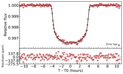
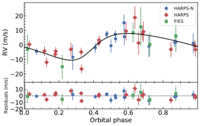
Figure 4: Top panel: Transit light curve folded to the orbital period of K2-280 b and residuals. The thick black line is the re-binned best-fitting transit model. The red points are the K2 data. Bottom panel: The RV curve of K2-280 b phase-folded to the orbital period of the planet. The best fitting solution is marked with a solid black line. HARPS-N, HARPS, and FIES data are shown with blue circles, red diamonds, and green squares, respectively. The lower panel shows the residuals to the best-fitting model.

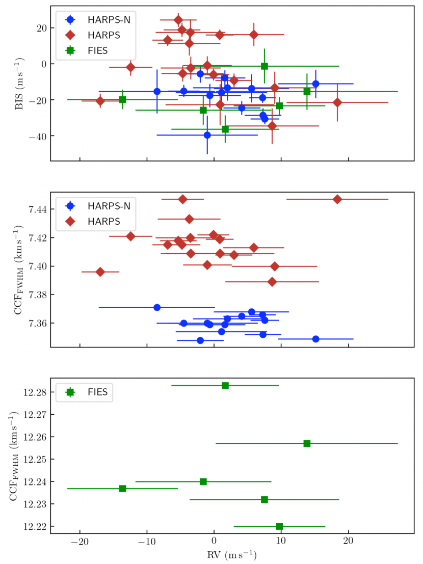
Figure 5: Top panel: The BIS versus RVs from HARPS-N, HARPS, and FIES. Middle panel: The $\mathrm{CCF_{FWHM}}$ versus RVs from HARPS-N and HARPS. Bottom panel: The $\mathrm{CCF_{FWHM}}$ versus RVs from FIES. RVs from all instruments have been subtracted by the systemic velocities listed in Table 5 and derived by our joint analysis.

The HARPS, HARPS-N, and FIES Doppler measurements show an RV variation in phase with the transit ephemeris (Figure 4, lower panel). However, as described by Cunha et al. (2013), contaminant stars that are within the sky-projected angular size of the spectrograph fibre (1″ for HARPS and HARPS-N, 1.3″ for FIES) may affect the radial velocity measurements of the target star. If the radial velocity of the contaminant star is changing, i.e., its spectrum is shifting across the spectrum of target star, it can distort the spectral line profile of the target (and hence its CCF), mimicking the presence of an orbiting planet. As presented by Cunha et al. (2013) in their Table 8, for magnitude differences of $\sim$5-6 mag, the impact of F2 V–K5 V contaminant star on a G8 V target star can be as high as 10 $\mathrm{m\,s^{-1}}$. If the nearby N–NW star, which has an angular separation $0.38\pm 0.011$″ from K2-280, is an F or G background eclipsing binary, it may not only generate a transit-like signal in the light curve of K2-280 every 19.9 days, but also a low-amplitude radial velocity signal at this period. We carefully checked the the FWHM and BIS of the HARPS, HARPS-N, and FIES cross-correlation functions to search for potential line profile variation induced by the blend companion. The generalized Lomb-Scargle periodograms (Zechmeister & Kürster, 2009) of these indicators show no significant signal neaither at the 19.9-day period and its harmonics, nor at any other period. We also found no correlation between the FWHM and BIS, and the RV measurements (Figure 5). In particular, the Spearman correlation coefficient between the HARPS RV measurements and the BIS of CCFs is equal to $r_{RV-BIS,HARPS}$ = -0.45 and between HARPS RVs and FWHM is equal to $r_{RV-FWHM,HARPS}$ = -0.18. The Spearman correlation coefficient between the HARPS-N RVs and BIS is equal to $r_{RV-BIS,HARPS-N}$ = -0.19 and between the HARPS-N RVs and FWHM is equal to $r_{RV-FWHM,HARPS-N}$ = -0.06. In the case of FIES measurements, the Spearman correlation coefficient between RVs and BIS is equal to $r_{RV-BIS,FIES}$ = 0.37 and between RVs and FWHM is equal to $r_{RV-FWHM,FIES}$ = -0.08.

We note that we could not measure the stellar rotation period from the K2 light curve. Using the stellar radius determined in Section 3.4 and the projected rotation velocity determined in Section 3.2, we found the upper limit of the stellar rotation period to be $P_{\mathrm{rot}}=21.6^{+12.6}_{-6.3}$ days. This means that the stellar rotation period of K2-280 is shorter than 34.2 days. Following the prescription given by Aigrain et al. (2012), the photometric variation found in the K2 light curve ($\sim$600 ppm) implies an activity induced RV signal of about 2 $\mathrm{m\,s^{-1}}$ (1.9 $\mathrm{m\,s^{-1}}$ for stellar rotation period equal to orbital period of K2-280 b (19.9 days) or 1.1 $\mathrm{m\,s^{-1}}$ for $P_{\mathrm{rot}}$ equal to 34.2 days). The probability that stellar rotation modulation may generate RV variations of K2-280 is therefore very low. We conclude that most likely the Doppler shift of K2-280 is induced by the orbital motion of a planet transiting K2-280 rather than a blended eclipsing binary or stellar rotation modulation. We stress however that the activity-induced RV signal at a level of $\sim$2 $\mathrm{m\,s^{-1}}$ is larger than the jitter terms listed in Table 5 and larger than the precision on our estimate of the Doppler semi-amplitude variation induced by the planet ($K$ = $9.18\pm 1.27$ ${\rm m\,s^{-1}}$). Therefore, we warn the reader that our semi-amplitude estimate might be affected by unaccounted for stellar activity.

Table 5: K2-280 Stellar and Planetary Parameters

Parameter	Prior(a)	Inferred value(b)
Model Parameters
Orbital period $P_{\mathrm{orb}}$ (days)	$\mathcal{U}[19.89,19.90]$	$19.89526\pm 0.00028$
Transit epoch $T_{0}$ (BJD${}_{\mathrm{TDB}}-$2 450 000)	$\mathcal{U}[7307.55,7307.65]$	$7307.58114\pm 0.00056$
Scaled semi-major axis $a/R_{\star}$	$\mathcal{N}[25.58,0.90]$	$25.79_{-0.90}^{+0.87}$
Scaled planet radius $R_{\mathrm{p}}/R_{\star}$	$\mathcal{U}[0,0.2]$	$0.05354_{-0.00056}^{+0.00094}$
Impact parameter, $b$	$\mathcal{U}[0,1]$	$0.27_{-0.17}^{+0.16}$
$\sqrt{e}\sin\omega_{\star}$	$\mathcal{U}[-1,1]$	$-0.547_{-0.05}^{+0.047}$
$\sqrt{e}\cos\omega_{\star}$	$\mathcal{U}[-1,1]$	$-0.235_{-0.043}^{+0.038}$
Radial velocity semi-amplitude variation $K$ (m s-1)	$\mathcal{U}[0,50]$	$9.18\pm 1.27$
Parameterized limb-darkening coefficient $q_{1}$	$\mathcal{U}[0,1]$	$0.54_{-0.11}^{+0.14}$
Parameterized limb-darkening coefficient $q_{2}$	$\mathcal{U}[0,1]$	$0.249_{-0.071}^{+0.082}$
Systemic velocity $\gamma_{\mathrm{HARPS-N}}$ (km s-1)	$\mathcal{U}[-2.2,-0.2]$	$-1.1934_{-0.0011}^{+0.0011}$
Systemic velocity $\gamma_{\mathrm{HARPS}}$ (km s-1)	$\mathcal{U}[-2.2,-0.2]$	$-1.1907_{-0.0011}^{+0.0011}$
Systemic velocity $\gamma_{\mathrm{FIES}}$ (km s-1)	$\mathcal{U}[-2.2,-0.2]$	$-1.2349_{-0.0039}^{+0.0038}$
Jitter term $\sigma_{\rm HARPS-N}$ (m s-1)	$\mathcal{U}[0,100]$	$0.36_{-0.3}^{+0.97}$
Jitter term $\sigma_{\rm HARPS}$ (m s-1)	$\mathcal{U}[0,100]$	$1.28_{-1.13}^{+1.76}$
Jitter term $\sigma_{\rm FIES}$ (m s-1)	$\mathcal{U}[0,100]$	$0.67_{-0.58}^{+2.58}$
Derived Parameters planet b
Planet mass $M_{\mathrm{p}}$ ($M_{\rm\oplus}$)	$\cdots$	$37.1\pm 5.6$
Planet radius $R_{\mathrm{p}}$ ($R_{\rm\oplus}$)	$\cdots$	$7.50\pm 0.44$
Planet density $\rho_{\mathrm{p}}$ (${\rm g\,cm^{-3}}$)	$\cdots$	$0.48_{-0.10}^{+0.13}$
Semi-major axis of the planetary orbit $a$ (au)	$\cdots$	$0.1461_{-0.0097}^{+0.0099}$
Orbital eccentricity, $e$	$\cdots$	$0.35_{-0.04}^{+0.05}$
Angle of Periastron, $\omega_{\star}$ (deg)	$\cdots$	$246.77_{-5.28}^{+4.54}$
Time of periastron $T_{\rm p}$ (BJD${}_{\mathrm{TDB}}-$2 450 000)	$\cdots$	$7315.06_{-0.44}^{+0.38}$
Transit duration $\tau_{14}$ (hours)	$\cdots$	$8.267_{-0.054}^{+0.063}$
Equilibrium temperature(c) $T_{\mathrm{eq}}$ (K)	$\cdots$	$787\pm 17$
Linear limb-darkening coefficient $u_{1}$	$\cdots$	$0.367_{-0.079}^{+0.074}$
Quadratic limb-darkening coefficient $u_{2}$	$\cdots$	$0.37_{-0.15}^{+0.15}$
Planet surface gravity(d) (${\rm cm\,s^{-2}}$)	$\cdots$	$648.0_{-102.0}^{+107.0}$
Planet surface gravity (${\rm cm\,s^{-2}}$)	$\cdots$	$647.0_{-117.0}^{+133.0}$

Note – ^(a) $\mathcal{U}[a,b]$ refers to uniform priors between $a$ and $b$, and $\mathcal{N}[a,b]$ to Gaussian priors with median $a$ and standard deviation $b$. ^(b) The inferred parameter value and its uncertainty are defined as the median and 68.3 percent credible interval of the posterior distribution. ^(c) Assuming albedo $=0$. ^(d) Calculated from the scaled-parameters as suggested by Southworth et al. (2007).

5 Discussion and Summary

5.1 K2-280 b and the current sample of sub-Saturn planets

With a mass of $M_{\mathrm{b}}$ = $37.1\pm 5.6$ $M_{\oplus}$ and a radius of $R_{\mathrm{b}}$ = $7.50\pm 0.44$ $R_{\oplus}$, K2-280 b joins the group of sub-Saturns planets – defined as planets having radii between 4 and 8 $\mathrm{R_{\oplus}}$ (Petigura et al., 2017) – whose masses and radii have been measured. The basic physical parameters of a sample of 23 sub-Saturns with densities measured with a precision better than 50% have been presented and discussed by Petigura et al. (2017). We here extend this sample by adding K2-280 b alongside 6 additional sub-Saturns that have densities measured with a precision better than 50%, as described below. WASP-156 b (Demangeon et al., 2018), a $\sim$0.5 $\mathrm{R_{\mathrm{Jup}}}$ planet with a Jupiter-like density was discovered by the ground-based SuperWASP transit survey (Pollacco et al., 2006; Smith & WASP Consortium, 2014). Kepler-1656 b, a dense sub-Saturn with a high eccentricity of $e$ = 0.84 transiting a relatively bright ($V=$ 11.6 mag) solar-type star, was recently reported by Brady et al. (2018). Three sub-Saturns were discovered and characterised by the KESPRINT consortium, two of them in K2 campaign 3 (K2-60 b, Eigmüller et al., 2017) and campaign 14 (HD 89345 b, aka K2-234 b, Van Eylen et al., 2018; Yu et al., 2018b), and HD 219666 b (Esposito et al., 2019) in TESS Sector 1. One sub-Saturn, GJ 3470 b (Bonfils et al., 2012), orbiting an M1.5 dwarf was not included by Petigura et al. (2017), but we add it to the current sample, adopting the parameters from Awiphan et al. (2016). All of these new sub-Saturns, including K2-280 b, reside in apparently single systems. Figure 6 shows the mass–radius and mass–density diagrams for this extended sample of 30 planets. Sub-Saturns found to be in multi-planet systems are marked with green filled circles, whereas those in single systems are marked with blue filled circles. The position of K2-280 b is indicated with a red-rimmed circle. Sub-Saturns whose density has been measured with a precision slightly worse than 50% are marked with green and blue open circles. All the remaining transiting planets with measured radii and masses are marked with open gray circles. According to the Fortney et al. (2007)’s models – also shown in the mass-radius diagram (Figure 6, upper panel) – K2-280 b has a core of about 10–25 $\mathrm{M_{\oplus}}$, accounting for $\sim$25–65% of its total mass.

The diagrams in Figure 6 confirm the main characteristics found by Petigura et al. (2017) for the population of sub-Saturns. One of the main property is the uniform distribution of masses in the range $\sim$5–75 $\mathrm{M_{\oplus}}$. With a mass of 135 $\pm$ 12 $\mathrm{M_{\oplus}}$ and radius of 7.66 $\pm$ 0.41 $\mathrm{R_{\oplus}}$, K2-60 b (Eigmüller et al., 2017) is close to the lower envelope of giant planets on the mass–radius diagram and is the only sub-Saturn-sized planet with a mass higher than Saturn (95.16 $\mathrm{M_{\oplus}}$). With a mean density of 1.7 $\pm$ 0.3 $\mathrm{g\,cm^{-3}}$ (i.e. Neptune’s density), K2-60 b is also the most dense planet in the mass range $\sim$75–250 $\mathrm{M_{\oplus}}$. As stressed by Eigmüller et al. (2017), K2-60 b with radius smaller than expected from the models of Laughlin et al. (2011) is more dense than expected and close to the sub-Jovian desert characterised by scarcity of planets with orbital periods below 4 days and masses lower than $\sim$300 $\mathrm{R_{\oplus}}$ (Szabó & Kiss, 2011; Beaugé & Nesvorný, 2013; Mazeh et al., 2016). The underestimation of its radius was excluded based on adaptive optics imaging (Schmitt et al., 2016). Only radial accelerations lower than 2 $\mathrm{m\,s^{-1}\,day^{-1}}$ that can not be excluded based on RVs collected by Eigmüller et al. (2017) suggest that mass of K2-60 b may be lower than current determination. Nevertheless, this intriguing planet may help with a study of sub-Jovian desert and its borders.

Although the mass distribution of sub-Saturns is quite uniform, the most massive ones have radii close to and below $\sim$6 $\mathrm{R_{\oplus}}$, visible as a correlation on the mass–density diagram (Figure 6, lower panel). The Spearman correlation coefficient between mass and density for the current sample of 30 sub-Saturns (excluding K2-60 b) is equal to $r$ = 0.72. This correlation is comparable to the one for the sample of 23 planets discussed in Petigura et al. (2017) that is equal to $r$ = 0.79. Notably, almost all of the most massive sub-Saturns from the current sample of 30 planets reside in apparently single-planet systems (blue circles in Figure 6). Sub-Saturns in single-planet systems have also often moderate eccentricities, higher than their counterparts in multi-planet systems, as shown in Figure 7. As suggested by Petigura et al. (2017), the moderate eccentricities of more massive sub-Saturns in apparently single systems and the lack of high-eccentricity, high-mass objects in multi-planet systems may be explained by scattering and merging events during the formation process.

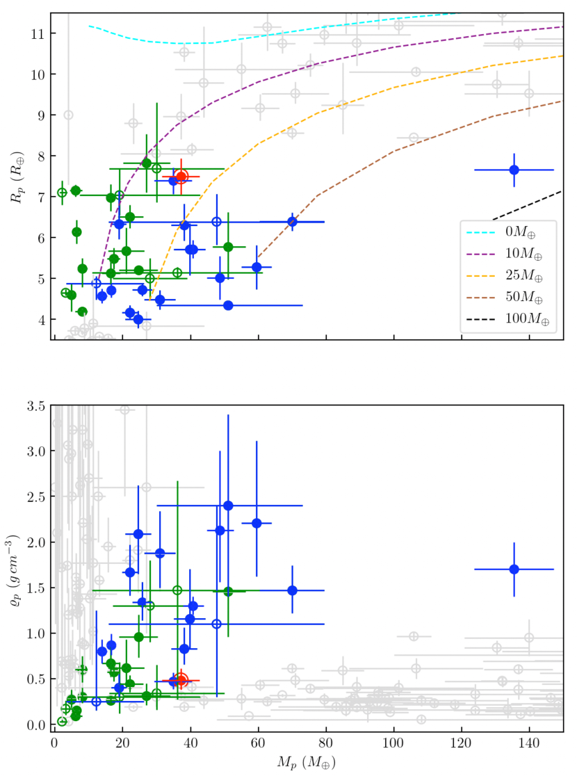
Figure 6: Mass–radius (upper panel) and mass–density (lower panel) diagrams for a sample of sub-Saturns ($R_{\mathrm{p}}\,=4-8\,\mathrm{R_{\oplus}}$). Sub-Saturns whose mean densities have been measured with a precision better than 50% located in multi-planet systems are marked with green filled circles, wheres those in single systems are marked with blue filled circles. The position of K2-280 b is indicated as a red-rimmed circle. Sub-Saturns with densities measured with a precision slightly worse than 50% are marked with green and blue open circles. The remaining planets with measured radii, masses and mean densities (NASA Exoplanet Archive (Akeson et al., 2013), as of July 2019) are marked with open gray circles. The dashed lines on the mass–radius diagram (upper panel) correspond to the Fortney et al. (2007) models for planet core masses of 0, 10, 25, 50, and 100 $\mathrm{M_{\oplus}}$ and age 10 Gyrs.

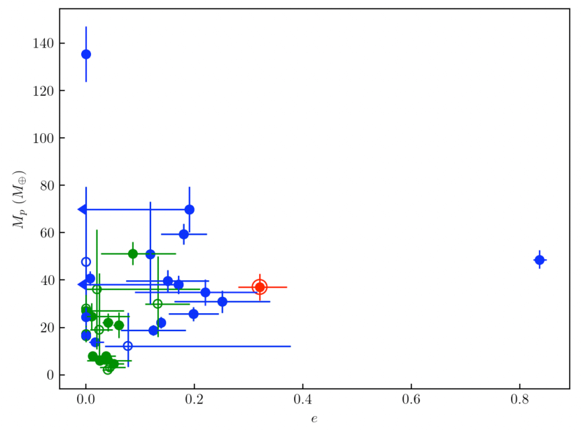
Figure 7: Mass of sub-Saturn planets as a function of the eccentricity. Samples and point symbols as in Figure 6.

Petigura et al. (2017) found a marginal correlation between the stellar metallicity and the mass of sub-Saturn planets (the Spearman correlation coefficient $r$ = 0.57), with the massive sub-Saturns found to orbit metal-rich stars. We confirm this for the current sample of 30 sub-Saturns (excluding K2-60 b) with exactly the same value of the Spearman correlation coefficient. This is consistent with the results of Buchhave et al. (2012) who, based on the sample of Kepler planets, found that planets larger than $\sim$4 $\mathrm{R_{\oplus}}$ orbit stars with relatively high metal content ($-$0.2 < [Fe/H] < 0.5 dex). For the sake of consistency with Figures 6 and 7, we included in Figure 8 the sub-Saturns orbiting binary stars, namely, Kepler-47 (AB) c and d ([Fe/H] = $-$0.25 $\pm$ 0.08 dex) and Kepler-413 (AB) b ([Fe/H] = $-$0.2 $\pm$ 0.1 dex), which were omitted by Petigura et al. (2017). Given its mass of $M_{\mathrm{p}}$ = $37.1\pm 5.6$ $M_{\oplus}$ and the iron content of its host star ($\mathrm{[Fe/H]}$ = ${0.33}\,{\pm}\,{0.08}$ $\mathrm{dex}$), K2-280 b follows this trend, being a relatively massive sub-Saturn orbiting a metal rich star.

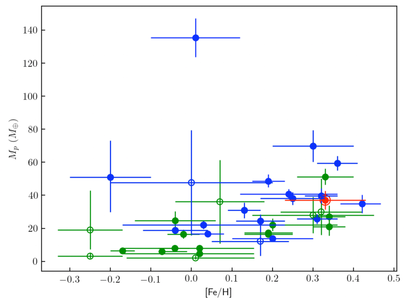
Figure 8: Mass of sub-Saturn planets as a function of iron content of their host stars. Samples and point symbols as in Figure 6.

K2-280 b has a relatively long orbital period of $\sim$19.9 days and transits a slightly evolved star in an apparently single-planet system. With an eccentricity of $e$ = $0.35_{-0.04}^{+0.05}$  , K2-280 b is exactly within the range of eccentricities found by Van Eylen et al. (2019) for Kepler systems with single transiting giant planets ($R_{\mathrm{p}}$ > 6 $\mathrm{R_{\oplus}}$). After Kepler-1656 b (Brady et al., 2018), K2-280 b is the second most eccentric sub-Saturn known to date. In contrast to Kepler-1656 b, the mass of $M_{\mathrm{b}}$ = $37.1\pm 5.6$ $M_{\oplus}$, radius of $R_{\mathrm{b}}$ = $7.50\pm 0.44$ $R_{\oplus}$, and mean density of $\rho_{\mathrm{b}}$ = $0.48_{-0.10}^{+0.13}$ ${\rm g\,cm^{-3}}$, make K2-280 b more similar to HD 89345 b (aka K2-234 b; Van Eylen et al., 2018; Yu et al., 2018b). The moderate eccentricity of K2-280 b suggests a formation pathway involving planet-planet gravitational interactions, and make this sub-Saturn planet a member of a relatively rare group of exoplanets and an interesting object for possible future follow-up.

5.2 Prospects for atmospheric characterisation and Rossiter-McLaughlin effect measurements

Although K2-280 b is a quite puffy planet, the relatively large radius of its host star ($R_{\star}$ =  $1.28\pm 0.07$ $R_{\odot}$) results in a quite low transmission signal per scale height ($H$) of the planetary atmosphere (55 ppm). This makes it a difficult target for atmospheric characterisation with current ground- and space-based facilities. The transmission spectroscopy metric (TSM) defined by Kempton et al. (2018) for JWST/NIRISS is $\sim$45 for K2-280 b, i.e. two times lower than the threshold TSM for planets with radii $R_{\mathrm{p}}\in(1.5-10.0)$ $\mathrm{R_{\oplus}}$ to be selected as high-quality atmospheric characterization targets. The long transit duration ($\sim$8 hours) further complicates ground-based follow-up observations.

Still, there is a possibility of Rossiter-McLaughlin (RM) effect measurements, for which the overall amplitude is expected to be $\sim$6 $\mathrm{m\,s^{-1}}$, depending on the real values of stellar projected rotation velocity and planetary and stellar radii. With an impact parameter of $b$ = $0.27_{-0.17}^{+0.16}$  , the transit of K2-280 b is close to being central. In such a case the shape of the RM effect would not change significantly with the sky-projected spin-orbit angle $\lambda$, but mainly the RM amplitude, leading to a strong correlation between $\lambda$ and $\mathit{v}_{\mathrm{rot}}\sin\,i_{\star}$ (see, e.g., Albrecht et al., 2011). Therefore more precise determination of $\mathit{v}_{\mathrm{rot}}\sin\,i_{\star}$ of this slow rotator, based for instance on the Fourier transform technique (e.g. Smith & Gray, 1976; Dravins et al., 1990; Gray, 2008, and references therein) applied to single very high resolution and high SNR line profiles, would be needed. Measurements of the sky-projected spin-orbit angle through RM observations may help to test formation scenarios of warm sub-Saturn planets. This gives additional arguments for attempting RM observations, as the probability of a misalignment between the planet’s orbital angular momentum vector and its host star’s spin axis should be higher if caused by a perturber than by primordial misalignment of the protoplanetary disk. Two full transits of K2-280 b  observable from the Chilean observatories will occur on July 7^th/8^th 2020 and August 9^th/10^th 2021.

6 Conclusions

We report here detailed characterisation of a low-density ($\rho_{\mathrm{b}}$ = $0.48_{-0.10}^{+0.13}$ ${\rm g\,cm^{-3}}$) sub-Saturn transiting a mildly evolved, metal rich G7 star K2-280. With a mass of $M_{\mathrm{b}}$ = $37.1\pm 5.6$ $M_{\oplus}$, a radius of $R_{\mathrm{b}}$ = $7.50\pm 0.44$ $R_{\oplus}$, and an eccentricity of $e$ = $0.35_{-0.04}^{+0.05}$  , K2-280 b joins the group of sub-Saturns planets in apparently single-planet systems. This second most eccentric sub-Saturn known to date is an interesting object for possible future follow-up observations that may help to test formation scenarios of this intriguing group of planets that are absent in the Solar System.

¹Instituto de Astrofísica de Canarias (IAC), 38205 La Laguna, Tenerife, Spain
²Departamento de Astrofísica, Universidad de La Laguna (ULL), 38206 La Laguna, Tenerife, Spain
³Dipartimento di Fisica, Universitá di Torino, Via P. Giuria 1, I-10125, Torino, Italy
⁴Department of Earth and Planetary Sciences, Tokyo Institute of Technology, 2-12-1 Ookayama, Meguro-ku, Tokio, Japan
⁵Sub-department of Astrophysics, Department of Physics, University of Oxford, Oxford OX1 3RH, UK
⁶Astrobiology Center, NINS, 2-21-1 Osawa, Mitaka, Tokyo 181-8588, Japan
⁷National Astronomical Observatory of Japan, NINS, 2-21-1 Osawa, Mitaka, Tokyo 181-8588, Japan
⁸Department of Astrophysical Sciences, Princeton University, 4 Ivy Lane, Princeton, NJ, 08544, USA
⁹Department of Physics and Kavli Institute for Astrophysics and Space Research, MIT, Cambridge, MA 02139, USA
¹⁰Chalmers University of Technology, Department of Space, Earth and Environment, Onsala Space Observatory, SE-439 92 Onsala, Sweden
¹¹Leiden Observatory, University of Leiden, PO Box 9513, 2300 RA, Leiden, The Netherlands
¹²Las Cumbres Observatory, 6740 Cortona Dr., Ste. 102, Goleta, CA 93117 USA
¹³Rheinisches Institut für Umweltforschung an der Universität zu Köln, Aachener Strasse 209, 50931 Köln, Germany
¹⁴Department of Astronomy, The University of Tokyo, 7-3-1 Hongo, Bunkyo-ku, Tokyo 113-0033, Japan
¹⁵Thüringer Landessternwarte Tautenburg, D-07778 Tautenburg, Germany
¹⁶Stellar Astrophysics Centre, Department of Physics and Astronomy, Aarhus University, Ny Munkegade 120, DK-8000 Aarhus C
¹⁷Center for Astronomy and Astrophysics, TU Berlin, Hardenbergstr. 36, 10623 Berlin, Germany
¹⁸Department of Astronomy and McDonald Observatory, University of Texas at Austin, 2515 Speedway, Austin, TX 78712, USA
¹⁹Institute of Planetary Research, German Aerospace Center (DLR), Rutherfordstrasse 2, D-12489 Berlin, Germany
²⁰Astronomical Institute, Czech Academy of Sciences, Fričova 298, 25165, Ondřejov, Czech Republic
${21}$Valencian International University (VIU), Pintor Sorolla 21, 46002 Valencia, Spain
²² Center of Astro-Engineering UC, Pontificia Universidad Católica de Chile,
²³Millennium Institute for Astrophysics, Av. Vicuña Mackenna 4860, 782-0436 Macul, Santiago, Chile
²⁴Instituto de Astrofísica, Pontificia Universidad Católica de Chile, Av. Vicuña Mackenna 4860, 782-0436 Macul, Santiago, Chile
²⁵Facultad de Ingeniería y Ciencias, Universidad Adolfo Ibáñez, Av. Diagonal las Torres 2640, Peñalolén, Santiago, Chile
${26}$Max-Planck-Institut für Astronomie, Königstuhl 17, 69117 Heidelberg, Germany
²⁷European Southern Observatory, Alonso de Córdova 3107, Vitacura, Casilla 19001, Santiago de Chile, Chile
²⁸Astronomy Department and Van Vleck Observatory, Wesleyan University, Middletown, CT 06459, USA
²⁹JST, PRESTO, 2-21-1 Osawa, Mitaka, Tokyo 181-8588, Japan
³⁰Department of Earth, Atmospheric and Planetary Sciences, MIT, 77 Massachusetts Avenue, Cambridge, MA 02139, USA
³¹Institut de Ciències de l’Espai (ICE, CSIC), Campus UAB,C/ de Can Magrans s/n, E-08193 Bellaterra, Spain
³²Institut d’Estudis Espacials de Catalunya (IEEC), C/ Gran Capitá 2-4, E-08034 Barcelona, Spain
³³Department of Theoretical Physics and Astrophysics, Masaryk University, Kotlářská 2, 61137 Brno, Czech Republic
³⁴Astronomical Institute, Faculty of Mathematics and Physics, Charles University, V Holešovičkách 2, 180 00, Praha, Czech Republic

Appendix A Corner plot for fitted parameters

Figure 9: Corner plot for the fitted parameters of the K2-280 system. This figure was created using corner.py (Foreman-Mackey, 2016).

References

- Aigrain et al. (2012) Aigrain S., Pont F., Zucker S., 2012, MNRAS, 419, 3147
- Akeson et al. (2013) Akeson R. L., et al., 2013, PASP, 125, 989
- Albrecht et al. (2011) Albrecht S., et al., 2011, ApJ, 738, 50
- Awiphan et al. (2016) Awiphan S., et al., 2016, MNRAS, 463, 2574
- Bailer-Jones et al. (2018) Bailer-Jones C. A. L., Rybizki J., Fouesneau M., Mantelet G., Andrae R., 2018, AJ, 156, 58
- Baranne et al. (1996) Baranne A., et al., 1996, A&AS, 119, 373
- Barragán & Gandolfi (2017) Barragán O., Gandolfi D., 2017, Exotrending: Fast and easy-to-use light curve detrending software for exoplanets (ascl:1706.001)
- Barragán et al. (2016) Barragán O., et al., 2016, AJ, 152, 193
- Barragán et al. (2018a) Barragán O., et al., 2018a, MNRAS, 475, 1765
- Barragán et al. (2018b) Barragán O., et al., 2018b, A&A, 612, A95
- Barragán et al. (2019) Barragán O., Gandolfi D., Antoniciello G., 2019, MNRAS, 482, 1017
- Beaugé & Nesvorný (2013) Beaugé C., Nesvorný D., 2013, ApJ, 763, 12
- Bonfils et al. (2012) Bonfils X., et al., 2012, A&A, 546, A27
- Borucki et al. (2010) Borucki W. J., et al., 2010, Science, 327, 977
- Brady et al. (2018) Brady M. T., et al., 2018, AJ, 156, 147
- Bressan et al. (2012) Bressan A., Marigo P., Girardi L., Salasnich B., Dal Cero C., Rubele S., Nanni A., 2012, MNRAS, 427, 127
- Bruntt et al. (2010) Bruntt H., et al., 2010, MNRAS, 405, 1907
- Buchhave et al. (2010) Buchhave L. A., et al., 2010, ApJ, 720, 1118
- Buchhave et al. (2012) Buchhave L. A., et al., 2012, Nature, 486, 375
- Burnham & Anderson (2002) Burnham K., Anderson D., 2002, Model Selection and Multimodel Inference: A Practical Information-Theoretic Approach. New York: Springer-Verlag
- Christiansen et al. (2017) Christiansen J. L., et al., 2017, AJ, 154, 122
- Coşkunoǧlu et al. (2011) Coşkunoǧlu B., et al., 2011, MNRAS, 412, 1237
- Cosentino et al. (2012) Cosentino R., et al., 2012, in Ground-based and Airborne Instrumentation for Astronomy IV. p. 84461V, doi:10.1117/12.925738
- Crossfield et al. (2016) Crossfield I. J. M., et al., 2016, ApJS, 226, 7
- Crossfield et al. (2018) Crossfield I. J. M., et al., 2018, ApJS, 239, 5
- Cunha et al. (2013) Cunha D., Figueira P., Santos N. C., Lovis C., Boué G., 2013, A&A, 550, A75
- Dai et al. (2017) Dai F., Winn J. N., Yu L., Albrecht S., 2017, AJ, 153, 40
- Demangeon et al. (2018) Demangeon O. D. S., et al., 2018, A&A, 610, A63
- Dorn et al. (2015) Dorn C., Khan A., Heng K., Connolly J. A. D., Alibert Y., Benz W., Tackley P., 2015, A&A, 577, A83
- Dotter et al. (2008) Dotter A., Chaboyer B., Jevremović D., Kostov V., Baron E., Ferguson J. W., 2008, ApJS, 178, 89
- Doyle et al. (2014) Doyle A. P., Davies G. R., Smalley B., Chaplin W. J., Elsworth Y., 2014, MNRAS, 444, 3592
- Dravins et al. (1990) Dravins D., Lindegren L., Torkelsson U., 1990, A&A, 237, 137
- Dressing et al. (2017) Dressing C. D., et al., 2017, AJ, 154, 207
- Eastman et al. (2010) Eastman J., Siverd R., Gaudi B. S., 2010, PASP, 122, 935
- Eigmüller et al. (2017) Eigmüller P., et al., 2017, AJ, 153, 130
- Esposito et al. (2019) Esposito M., et al., 2019, A&A, 623, A165
- Foreman-Mackey (2016) Foreman-Mackey D., 2016, The Journal of Open Source Software, 1, 24
- Fortney et al. (2007) Fortney J. J., Marley M. S., Barnes J. W., 2007, ApJ, 659, 1661
- Frandsen & Lindberg (1999) Frandsen S., Lindberg B., 1999, in Karttunen H., Piirola V., eds, Astrophysics with the NOT. p. 71
- Fridlund et al. (2017) Fridlund M., et al., 2017, A&A, 604, A16
- Gaia Collaboration et al. (2016) Gaia Collaboration et al., 2016, A&A, 595, A1
- Gaia Collaboration et al. (2018) Gaia Collaboration et al., 2018, A&A, 616, A1
- Gandolfi et al. (2008) Gandolfi D., et al., 2008, ApJ, 687, 1303
- Gandolfi et al. (2015) Gandolfi D., et al., 2015, A&A, 576, A11
- Gandolfi et al. (2017) Gandolfi D., et al., 2017, AJ, 154, 123
- Gelman & Rubin (1992) Gelman A., Rubin D. B., 1992, Statistical Science, 7, 457
- Gray (2008) Gray D. F., 2008, The Observation and Analysis of Stellar Photospheres
- Gray & Corbally (2009) Gray R. O., Corbally J. C., 2009, Stellar Spectral Classification
- Hekker et al. (2006) Hekker S., Reffert S., Quirrenbach A., Mitchell D. S., Fischer D. A., Marcy G. W., Butler R. P., 2006, A&A, 454, 943
- Hekker et al. (2008) Hekker S., Snellen I. A. G., Aerts C., Quirrenbach A., Reffert S., Mitchell D. S., 2008, A&A, 480, 215
- Hirano et al. (2018) Hirano T., et al., 2018, AJ, 155, 127
- Hjorth et al. (2019) Hjorth M., et al., 2019, MNRAS, 484, 3522
- Hodapp et al. (2003) Hodapp K. W., et al., 2003, PASP, 115, 1388
- Howell et al. (2014) Howell S. B., et al., 2014, PASP, 126, 398
- Jenkins et al. (2010) Jenkins J. M., et al., 2010, ApJ, 713, L87
- Johnson & Soderblom (1987) Johnson D. R. H., Soderblom D. R., 1987, AJ, 93, 864
- Kempton et al. (2018) Kempton E. M. R., et al., 2018, PASP, 130, 114401
- Kipping (2010) Kipping D. M., 2010, MNRAS, 408, 1758
- Kovács et al. (2002) Kovács G., Zucker S., Mazeh T., 2002, A&A, 391, 369
- Kurucz (2013) Kurucz R. L., 2013, ATLAS12: Opacity sampling model atmosphere program, Astrophysics Source Code Library (ascl:1303.024)
- Laughlin et al. (2011) Laughlin G., Crismani M., Adams F. C., 2011, ApJ, 729, L7
- Livingston et al. (2018) Livingston J. H., et al., 2018, AJ, 156, 277
- Luri et al. (2018) Luri X., et al., 2018, A&A, 616, A9
- Malavolta et al. (2018) Malavolta L., et al., 2018, AJ, 155, 107
- Mandel & Agol (2002) Mandel K., Agol E., 2002, ApJ, 580, L171
- Mayer et al. (2005) Mayer L., Wadsley J., Quinn T., Stadel J., 2005, MNRAS, 363, 641
- Mayo et al. (2018) Mayo A. W., et al., 2018, AJ, 155, 136
- Mayor et al. (2003) Mayor M., et al., 2003, The Messenger, 114, 20
- Mazeh et al. (2016) Mazeh T., Holczer T., Faigler S., 2016, A&A, 589, A75
- Montet et al. (2015) Montet B. T., et al., 2015, ApJ, 809, 25
- Nelson (2000) Nelson A. F., 2000, ApJ, 537, L65
- Ofir (2014) Ofir A., 2014, A&A, 561, A138
- Pepe et al. (2013) Pepe F., et al., 2013, Nature, 503, 377
- Persson et al. (2018) Persson C. M., et al., 2018, A&A, 618, A33
- Petigura et al. (2016) Petigura E. A., et al., 2016, ApJ, 818, 36
- Petigura et al. (2017) Petigura E. A., et al., 2017, AJ, 153, 142
- Petigura et al. (2018) Petigura E. A., et al., 2018, AJ, 155, 21
- Piskunov & Valenti (2017) Piskunov N., Valenti J. A., 2017, A&A, 597, A16
- Pollacco et al. (2006) Pollacco D. L., et al., 2006, PASP, 118, 1407
- Prieto-Arranz et al. (2018) Prieto-Arranz J., et al., 2018, A&A, 618, A116
- Reddy et al. (2006) Reddy B. E., Lambert D. L., Allende Prieto C., 2006, MNRAS, 367, 1329
- Robin et al. (2003) Robin A. C., Reylé C., Derrière S., Picaud S., 2003, A&A, 409, 523
- Rodriguez et al. (2018) Rodriguez J. E., Vanderburg A., Eastman J. D., Mann A. W., Crossfield I. J. M., Ciardi D. R., Latham D. W., Quinn S. N., 2018, AJ, 155, 72
- Schmitt et al. (2016) Schmitt J. R., et al., 2016, AJ, 151, 159
- Smith & Gray (1976) Smith M. A., Gray D. F., 1976, PASP, 88, 809
- Smith & WASP Consortium (2014) Smith A. M. S., WASP Consortium 2014, Contributions of the Astronomical Observatory Skalnate Pleso, 43, 500
- Southworth et al. (2007) Southworth J., Wheatley P. J., Sams G., 2007, MNRAS, 379, L11
- Szabó & Kiss (2011) Szabó G. M., Kiss L. L., 2011, ApJ, 727, L44
- Tayar et al. (2019) Tayar J., Stassun K. G., Corsaro E., 2019, ApJ, 883, 195
- Telting et al. (2014) Telting J. H., et al., 2014, Astronomische Nachrichten, 335, 41
- Thébault et al. (2006) Thébault P., Marzari F., Scholl H., 2006, Icarus, 183, 193
- Torres et al. (2010) Torres G., Andersen J., Giménez A., 2010, A&ARv, 18, 67
- Udry et al. (1999) Udry S., Mayor M., Queloz D., 1999, in Hearnshaw J. B., Scarfe C. D., eds, Astronomical Society of the Pacific Conference Series Vol. 185, IAU Colloq. 170: Precise Stellar Radial Velocities. p. 367
- Valenti & Fischer (2005) Valenti J. A., Fischer D. A., 2005, ApJS, 159, 141
- Valenti & Piskunov (1996) Valenti J. A., Piskunov N., 1996, A&AS, 118, 595
- Van Eylen & Albrecht (2015) Van Eylen V., Albrecht S., 2015, ApJ, 808, 126
- Van Eylen et al. (2018) Van Eylen V., et al., 2018, MNRAS, 478, 4866
- Van Eylen et al. (2019) Van Eylen V., et al., 2019, AJ, 157, 61
- Vanderburg et al. (2015) Vanderburg A., et al., 2015, ApJ, 800, 59
- Vanderburg et al. (2016) Vanderburg A., et al., 2016, ApJS, 222, 14
- Vogt et al. (1994) Vogt S. S., et al., 1994, in Crawford D. L., Craine E. R., eds, Society of Photo-Optical Instrumentation Engineers (SPIE) Conference Series Vol. 2198, Proc. SPIE. p. 362, doi:10.1117/12.176725
- Winn et al. (2018) Winn J. N., Sanchis-Ojeda R., Rappaport S., 2018, New Astron. Rev., 83, 37
- Yee et al. (2017) Yee S. W., Petigura E. A., von Braun K., 2017, ApJ, 836, 77
- Yu et al. (2018a) Yu L., et al., 2018a, AJ, 156, 22
- Yu et al. (2018b) Yu L., et al., 2018b, AJ, 156, 127
- Zechmeister & Kürster (2009) Zechmeister M., Kürster M., 2009, A&A, 496, 577