Narrow-escape time and sorting of active particles in circular domains

Abstract

It is now well established that microswimmers can be sorted or segregated fabricating suitable microfluidic devices or using external fields. A natural question is how these techniques can be employed for dividing swimmers of different motility. In this paper, using numerical simulations in the dilute limit, we investigate how motility parameters (time of persistence and velocity) impacts the narrow-escape time of active particles from circular domains. We show that the escape time undergoes a crossover between two asymptotic regimes. The control parameters of the crossover is the ratio between persistence length of the active motion and the typical length scale of the circular domain. We explore the possibility of taking advantage of this finding for sorting active particles by motility parameters.

I Introduction

Active particles are widespread in nature Bechinger et al. (2016); Marchetti et al. (2013). Because of their autonomous motion, active particles break fluctuation-dissipation theorem at single-particle level Maggi et al. (2017) making possible a rich phenomenology that does not share any similarity with equilibrium systems Zhang et al. (2010); Lushi et al. (2014); Bricard et al. (2013); Sanchez et al. (2012). During the last decades, it has been shown that active particles and swimming organisms can be employed for actuating micro-motors Angelani et al. (2009); Di Leonardo et al. (2010); Sokolov et al. (2010); Maggi et al. (2016) , controlling and stabilizing density fluctuations Galajda et al. (2007); Bricard et al. (2013), or for driving macroscopic directed motion Angelani et al. (2011); Reichhardt and Reichhardt (2017). Many aspects of this remarkably phenomenology can be rationalized starting from the morphological properties of the single-particle trajectory. The typical trajectory of an active particle is well captured by a persistent random walk. In particular, the existence of a finite persistence length gives rise to a motion that is ballistic on a short-time scale and it becomes diffusive for larger times. It is now well established that, because of the finite persistency, active particles slow down in regions where they are denser Schnitzer (1993) and accumulate at the boundaries of a confining container Vladescu et al. (2014); Das et al. (2018). Remarkably, simple artificial environments can be designed for sorting active particles in small regions of space Galajda et al. (2007). However, sorting particles dynamically from slower to faster remains a challenge Mijalkov and Volpe (2013). While some attempts to obtain particles segregation have been made by using external fields Kaiser et al. (2012); Costanzo et al. (2014); Kumar et al. (2019), designing machinery suitable for segregating particles of different motility properties without using any external potential could have important applications, as in the case of in vitro fertilization where the identification and gathering of motile sperms without invasive techniques is a hard task Nosrati et al. (2017); Koh et al. (2015); Gaffney et al. (2011); Campana et al. (1996).

In this work, we will focus our attention on the narrow-escape problem of active particles Bénichou and Voituriez (2014); Singer et al. (2006a). We are interested in studying this problem numerically in two dimensions considering a circular container with a small target exit site on the boundary. The target site allows particles to escape from the confining structure and we assume that the particles cannot come back into the chamber. Looking at the properties of the first-passage time for a particle to escape from the chamber, we compare two paradigmatic active dynamics, i. e., Run-and-Tumble and Active Brownian. In agreement with recent studies on optimal search strategies with active particles Rupprecht et al. (2016), both the active dynamics show a crossover between two regimes in the mean first-passage time. The first regime, typical of active systems, takes place when the persistence length of the random walk is larger than the size of the confining structure. The second regime is reached in the diffusive limit, i. e., when the persistence length is small when compared with the size of the chamber.

Our findings show that, although both dynamics show exactly the same diffusive limit, in the active limit the comparison of different active dynamics at equal persistence times show up differences, with Run-and-Tumble particles being less efficient than Active Brownian in escaping from the chamber. We identify an empirical function $f(x)$ that matches smoothly the two regimes, with $x=\ell/R$, being $\ell$ the persistence length of the active motion and $R$ the radius of the confining structure. The function captures the crossover between the two scaling regimes that takes place for $x\approx 1$.

Since the two regimes can be reached in either way, by varying the motility parameters or by tuning the size of the confining structure, we show that one can take advantage of the crossover between active and diffusive regime for sorting particles of different persistence length by varying the size of the structure.

II Model and Methods

Figure 1: Active particles escaping from circular domains. A representative trajectory for a single Run-and-Tumble particle (a) and a single Active Brownian particle (b). The parameters are $\lambda=D_{r}=1,v_{self}=1,R=10(2\sigma){\color[rgb]{0,0,0}=10}$ Colors change from red to blue as time increases. In both cases the particle is injected at the center of the chamber and escapes from the circular domain, reaching a slit of width $\delta$ symmetrically displaced around $(R,0)$.

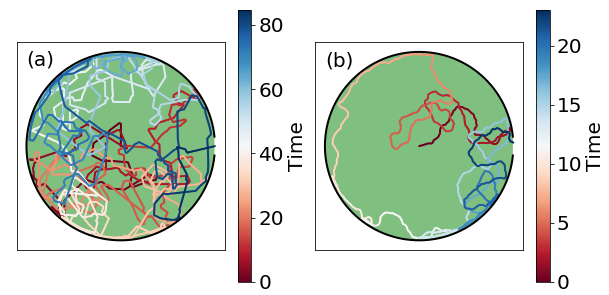
As a model system, we consider a gas of $N$ non-interacting active particles in two spatial dimensions confined to stay inside a circular chamber of radius $R$. The chamber has a slit of size $\delta$ on the boundary where particles can escape (they never come back). Indicating with $O=(0,0)$ the center of the chamber, the slit is displaced symmetrically around $(R,0)$, i. e., with coordinates $(R\cos\varphi,R\sin\varphi)$ and $(R\cos\varphi,-R\sin\varphi)$, with $\varphi=\delta/2R$. In the present work, we present results for a fixed value of $\delta=2\sigma$, with $\sigma$ the particle radius Paoluzzi et al. (2015), see below.

Figure 2: Mean First-Passage Time of active walkers escaping from circular domains. $\tau_{FPT}$, in unit of persistence time $\tau_{pers}$ (which is $1/\lambda$ or $1/D_{r}$ for Run-and-Tumble or Active Brownian particles respectively), is reported against the nondimensional parameter $\ell^{2}/R^{2}$, for Active Brownian (a) and Run-and-Tumble (b) particles. Square (diamonds) indicate results with an initial position set at the center of the chamber (uniformly distributed in the chamber). (c) Comparison between Run-and-Tumble and Active Brownian dynamics. The persistence length is varied by exploring different motility parameters, i. e., $\tau_{pers}\in[10^{-3},10]$, $v_{self}\in[10^{-2},10^{3}]$, and also by changing the chamber size, i. e., $R\in[5,8\times 10^{2}]$. The red lines are fit to the empirical function $f(x)$, see text, Eq. (3). The green curve in (c) is Eq. (4).

Figure 3: (a) Mean First-Passage Time as a function of the nondimnesional $\ell^{2}/R^{2}$ for different chamber sizes ranging from $R=5$ to $R=8\times 10^{2}$. (b) Mean First-Passage Time of reaching the boundary, the green curve is Eq. (3), for comparison we include Eq. (4) as a guide to the eye (red curve).

The confining structure is implemented through the image technique, i. e., the active particle sees its own image located at $R+2\sigma$, this choice ensures that the particle is point-like and it is confined to displace at distances smaller or equal to $R$ Paoluzzi et al. (2015). Each particle does not interact with the others. It is worth noting that the active walkers are point-like. However, since we are modeling the mechanical interaction with the confining walls using the image technique, the distance between the point-like particle and the force center of its image naturally introduce the length scale $\sigma$. In the following, we express length in unit of $2\sigma$. For the active dynamics, we consider two microscopic models: Run-and-Tumble and Active Brownian. Run-and-Tumble dynamics has been implemented following Refs. Angelani et al. (2009); Paoluzzi et al. (2014, 2013, 2018). Considering the case of overdamped dynamics, that is a good approximation at low Reynolds number, the equation of motion for the particle $i$ is

$$\dot{{\mathbf{r}}}_{i}(t)=v_{self}{\hat{\mathbf{e}}}_{i}+\mu{\mathbf{f}}_{image}\;.$$ (1)

The versor $\mathbf{e}_{i}=(\cos\theta_{i},\sin\theta_{i})$ specifies the swimming direction. $\mu=1$ is the mobility, ${\mathbf{f}}_{image}$ is the short-range force exerted by the image, i. e., ${\mathbf{f}}_{image}=-\nabla\phi(r_{image})$ with $\phi(r)=Ar^{-12}$ Angelani et al. (2009). The evolution of ${\hat{\mathbf{e}}}_{i}$ depends on the model we consider. In the case of Run-and-Tumble dynamics Schnitzer (1993), ${\hat{\mathbf{e}}}_{i}$ stochastically rotates with a rate $\lambda$, i. e., the tumbling rate. Meaning that a new orientational angle $\theta$ is extracted by a uniform distribution in $[0,2\pi]$ and then it remains constant for a time that is poissonian distributed with rate $\lambda$. For Active Brownian particles Das et al. (2018), the angle $\theta_{i}$ undergoes the following Langevin dynamics

$$\dot{\theta}_{i}(t)=\eta_{i}$$ (2)

with $\langle\eta_{i}(t)\rangle=0$ and $\langle\eta_{i}(t)\eta_{j}(s)=2D_{r}\delta_{ij}\delta(t-s)$, with $D_{r}$ the rotational diffusion constant.

The tumbling rate $\lambda$ and the diffusion coefficient $D_{r}$ fix $\tau_{pers}$ that is $\tau_{pers}=\lambda^{-1}$, and $\tau_{pers}=D_{r}^{-1}$, for the two active dynamics, respectively. Using the self-propulsion velocity $v_{self}$, we can define the persistence length $\ell=v_{self}\tau_{pers}$. In both cases, the motion is characterized by a ballistic regime on times $t\ll\tau_{pers}$ and a diffusive regime for $t\gg\tau_{pers}$. In two spatial dimensions, the diffusion can be described through the effective diffusion coefficient $D_{eff}=v_{self}^{2}\tau_{pers}/2$. We explore a wide range of persistence length by varying motility parameters $\tau_{pers}\in[10^{-3},10]$, $v_{self}\in[10^{-2},10^{3}]$. The chamber size is changed within the interval $R\in[5,8\times 10^{2}]$.

We solve Eq. (1) numerically integrating the equation of motion using Euler method with a time step $\Delta t$ ranging from $10^{-3}$ to $10^{-5}$. The numerical integration is performed until each of the runners has reached the target. In the first part of our work, we consider a gas of non-interacting active particles with same motility parameters $v_{self}$ and $\tau_{pers}$. Particles are injected in the center of the chamber at $t=0$ and thus the initial density profile $n({\mathbf{r}},0)$ reads $n({\mathbf{r}},0)=\frac{N}{\pi R^{2}}\delta({\mathbf{r}})$. We also consider the situation where particles are uniformly distributed at $t=0$. With both kinds of initial conditions we evaluate the Mean First-Passage Time $\tau_{FPT}$ defined as the average time required for escaping from the chamber. $\tau_{FPT}$ is computed considering the escape of $N=10^{5}$ particles.

In the second part we consider a mixture of particles injected in the center, with motility parameters ($v_{self}$ or $\tau_{pers}$) extracted from a uniform distribution. In this case, we are interested in the evolution of $n(v,t)$ and $n(D_{r},t)$ with $n(.,t)\equiv N(.,t)/N(.,0)$ and $N(.,t)$ the number of particles at time $t$ with a given value of motility parameters.

III Escape of a population with identical parameters

The typical trajectories of Run-and-Tumble and Active Brownian dynamics are shown in Fig. (1). Both dynamics share the same motility parameters, i. e., $\lambda=D_{r}=1$ and $v_{self}=1$. Particles are confined into a circular chamber of radius $R=10(2\sigma){\color[rgb]{0,0,0}=10}$. As one can see, in either cases, the typical trajectory is a persistent random walk, as it is well known in the literature Bechinger et al. (2016). Active Brownian dynamics generate smoother trajectories compared with those obtained through Run-and-Tumble. The latter are characterized by straight run interrupted by tumbling events. Because of the confinement, one expects to observe different dynamical behaviors depending on the characteristic size of the circular chamber. In particular, we define the active regime when the radius $R$ is smaller than the persistence length $\ell$. We thus identify the opposite situation as the diffusive regime, i. e., when $R\gg\ell$.

It is worth noting that a given value of $D_{eff}$ can be obtained through different combinations of $v_{self}$ and $\tau_{pers}$. Moreover, the genuine diffusive limit is recovered performing simultaneously the limit $v_{self}\to\infty$ and $\tau_{pers}\to 0$ at fixed $D_{eff}$, as it was realized by Kac in a seminal paper on the telegrapher’s equation Kac (1974). As we will see in the next section, both models show the same diffusive limit that is consistent with the dynamics of a Brownian walker coupled to a thermal bath with effective temperature $T_{eff}=\mu D_{eff}$. To conclude this overview of model parameters, we recall that $2D_{eff}\tau_{pers}/R^{2}=\ell^{2}/R^{2}$, therefore fixing (at given $R$) $\tau_{pers}$ and $\ell$ also fixes $D_{eff}$. Most importantly, the condition $R\ll\ell$ ($R\gg\ell$) is equivalent to $D_{eff}\tau_{pers}\gg R^{2}$ ($D_{eff}\tau_{pers}\ll R^{2}$).

Also in the active regime, $\tau_{FPT}$ follows the same asymptotic scaling behavior in both models. However, the fact that Run-and-Tumble and Active Brownian trajectories are morphologically different has a quantitative impact on $\tau_{FPT}$ away from the diffusive limit. This result is consistent with escape time of active particles from a maze Khatami et al. (2016).

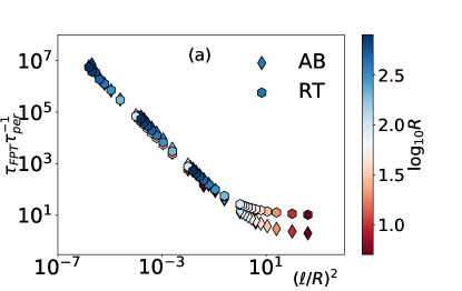
The mean first-passage time $\tau_{FPT}$ is shown in Fig. (2), rescaled by the persistence time $\tau_{pers}$. Following the previous discussion, as non-dimensional control parameter we use $(\ell/R)^{2}\equiv{\color[rgb]{0,0,0}2}D_{eff}\tau_{pers}/R^{2}$. Here we are considering a situation where the persistence length is changed by varying both the motility parameters, i. e., the persistence time $\tau_{pers}$, and the self-propulsion velocity $v_{self}$ (therefore different values of $D_{eff}$ are considered). Panel (a) referes to Active Brownian, panel (b) to Run-and-Tumble. We have also varied the radius $R$ of the chamber, see Panel (c).

The result is a collapse of data onto a master curve which is similar but not identical for the two dynamics. In both dynamics $\tau_{FPT}/\tau_{pers}$ undergoes a crossover from large values at small persistence length (diffusive regime) to small values at large persistence length (active regime). The color code indicates the inverse of the values of the persistence time $\tau_{pers}$. We have also reported data obtained with a different initial condition (diamonds in figure). In this case, the starting position is uniformly distributed and the results neatly superimpose on the master curve.

On a more quantitative level, we see that the diffusive regime, $\ell\ll R$ ($D_{eff}\tau_{pers}\ll R^{2}$), is signaled by a scaling $\tau_{FPT}/\tau_{pers}\sim(\ell/R)^{-2}=R^{2}/(D_{eff}\tau_{pers})$ which implies $\tau_{FPT}\sim R^{2}/D_{eff}$. In the opposite limit, i. e., $\ell\gg R$, where the active regime dominates, we observe a scaling $\tau_{FPT}\sim\tau_{pers}$.

In panel (c) of the same figure we compare the master curves for the Run-and-Tumble and Active Brownian dynamics. In this case, we are varying only the persistence time $\tau_{pers}$, i. e., the tumbling rate $\lambda$, in the case of Run-and-Tumble particles, and the rotational diffusion $D_{r}$, for Active Brownian particles. The diffusion limit is thus approached for $\tau_{pers}\to 0$, the active limit as soon as $\tau_{pers}\to\infty$. As one can see, they reach exactly the same diffusive limit when $D_{eff}R^{-2}\to 0$. In the opposite limit, i. e., $D_{eff}R^{-2}\to\infty$, $\tau_{FPT}\sim\tau_{pers}$, however, Run-and-Tumble particles are systematically slower in finding the exit than Active Brownian particles. We can guess that this difference is due to the fact that Active Brownian particles, at variance with Run-and-Tumble, smoothly change their self-propulsion direction.

The behavior observed in the active regime is consistent with optimal research strategies of run-and-tumble in spherical confinement Rupprecht et al. (2016). The divergence of $\tau_{FPT}$ with the persistence time can be rationalized noticing that, when $\tau_{pers}\to\infty$, only the walkers moving towards the right direction, i. e., with $\theta\in[-\varphi,\varphi]$, can escape from the chamber, therefore the escape becomes more and more difficult. However analytical predictions of $\tau_{FPT}$ for active dynamics remains an open problem Rupprecht et al. (2016); Redner (2001); Bénichou and Voituriez (2014); Singer et al. (2006b, a); Rupprecht et al. (2015). For the diffusive regime ($R\gg\ell$) the boundary is so far that active particles displace a distance $\langle\Delta x^{2}\rangle=D_{eff}t$ and thus the boundary is reached on a time scale $R^{2}/D_{eff}$, as we observe.

Noticeably, these two asymptotic regimes match smoothly at $\ell\,R^{-1}=1$. Indicating with $x=\ell^{2}R^{-2}$ the control parameter, we thus propose the following empirical function $f(x)$ that results suitable for capturing the whole emerging phenomenology of the nondimensional quantity $\tau_{FPT}/\tau_{pers}$

$$f(x)=\frac{\alpha}{x}+\beta,$$ (3)

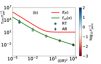
with $\alpha$ and $\beta$ which in principle may depend upon $R$. For instance in Rupprecht et al. (2016) (where the geometry has important differences with our setup) $\alpha\sim\log(R/\delta)$ and $\beta\sim R/\delta$. Here we find $\alpha=10.3$ and $\beta=2.0$ for Active Brownian particles at $R=10$ and $\alpha=8.5$ and $\beta=11.9$ for Run-and-Tumble particles at $R=10$. It is worth noting that, for the space of parameters explored here, the parameters $\alpha$ and $\beta$ turns out to be almost independent of $R$, as it is shown in Fig. (3)-(a). Just for comparison, in the one dimensional case one has the exact expression for the mean first-passage time Angelani et al. (2014); Angelani (2015)

$$f_{1d}(x)=1/2x+1/\sqrt{x}\;.$$ (4)

However, we note that this expression is obtained considering a particle which reaches for the first time the boundary points, corresponding in our two-dimensional case to a particle that escapes once reaching the circular boundary, i.e., $\delta=2\pi R$. As one can see in Fig. (3)-(b), where we computed the escape time for reaching the boundary, $f_{1d}(x)$ reproduces the numerical data. At large persistence lengths ($x\gg 1$) the time to hit the boundary is dominated by the term $\sim 1/\sqrt{x}\sim 1/v_{self}$, as expected for a purely ballistic motion. This behavior is quite different from that seen at large $x$ in Fig. 2, i.e. for the narrow escape problem: curve $f_{1d}(x)$ is plotted in Fig. 2c for comparison.

These findings show that particles moving in an environment characterized by a length scale $R>\ell$ are dramatically disadvantaged in finding the exit with respect to particles such that $R<\ell$. As we will show in the next section, this observation can be employed for the purpose of sorting particles with different persistent lengths.

Figure 4: Mixture of particles with different velocities. Time evolution of $n(v,t)$ at five representative times, the radius of the chamber is $R=1$ and rotational diffusion $D_{r}=1$. The initial distribution that is uniform in the interval $v\in[0.5,1.5]$. Faster particles with $v>1$ escape very early from the circular vessel.

IV Designing simple sorting devices

Figure 5: Decay of the number density for different $v_{self}$. (a) Time evolution of $n(v,t)$, velocity decreases from $1.5$ (dark red) to $0.5$ (light red) The decay of $n(v,t)$ is well captured by an exponential curve (dashed blue lines are fit with $n_{fit}(v,t)=Ae^{-t/\tau(v)}$ ). Inset: same observable for $R=10$. (b) The decay time $\tau(v)$ computed by fitting to an exponential decay (blue diamonds) and using Eq. (8) with $R=1$. Solid red curve is the empirical function $f(x)$ (in the inset $R=10$).

In this section we explore the possibility of tuning the geometrical properties of the confining structure for sorting particles of different velocities. The advantage of this approach relies on the fact that (i) we do not have to introduce any external field, (ii) the geometry is extremely simple and easily realised in microfluidics, as compared to  Galajda et al. (2007), (iii) the only parameter we have to tune is the radius $R$.

According to the results of the previous sections, $\tau_{FPT}$ shows a crossover around $R\ell^{-1}=1$ between two regimes characterized by different scaling laws. To make it explicit, we rewrite here Eq. (3) in terms of the motility parameters for the mean exit time:

$$\tau_{FPT}=\alpha\frac{R^{2}}{v_{self}^{2}\tau_{pers}}+\beta\tau_{pers}.$$ (5)

It is immediately understood that changing $v_{self}$ at constant $\tau_{pers}$ leads to a monotone behavior, with a crossover at $v_{self}\approx v_{self}^{*}$, with $v_{self}^{*}=\sqrt{\alpha/\beta}R/\tau_{pers}$, from a diffusive regime with slow escape to the active regime with fast escape. On the contrary, changing $\tau_{pers}$ at constant $v_{self}$ produces a non-monotone behavior with an optimal escape at $\tau_{pers}\approx\tau_{pers}^{*}$, with $\tau_{pers}^{*}=\sqrt{\alpha/\beta}R/v_{self}$ and slower escape both form smaller and larger values of $\tau_{pers}$. In both cases we foresee applications in sorting problems, with different ways of use.

IV.1 Different propulsion velocities

As a model system, we start by considering a gas composed by particles with different self-propulsion velocity. The velocity is extracted by a uniform distribution. We consider a system composed by $N=5\times 10^{4}$ Active Brownian particles in a circular chamber of size $R=1$ where a small slit of size $\delta={\color[rgb]{0,0,0}2\sigma}=1$ allows particles to escape. The system is characterized by the initial distribution of self-propulsion velocities $\rho(v)=\frac{1}{v_{max}-v_{min}}\left[\vartheta(v-v_{min})-\vartheta(v-v_{max})\right]$, with $\vartheta(x)$ the Heaviside step function. Here $v_{max}=1.5$ and $v_{min}=0.5$. All particles have the same rotational diffusion constant $D_{r}=\tau_{pers}^{-1}=1$. In this way, each particle $i$ has its own persistence length $\ell_{i}=v_{self}^{i}$. According to previous results we expect a crossover at $v_{self}^{*}\approx 1$: faster particles escape within a time of order $1$ on average, slower particles escape in a much slower time, sensitive upon $v_{self}$.

Figure 6: Mixture of particles with different persistence times. Time evolution of $n(D_{r},t)$ at six representative times, the radius of the chamber is $R=1$. The initial distribution $n(D_{r},0)$ is uniform in the interval $D_{r}\in[0,2]$.

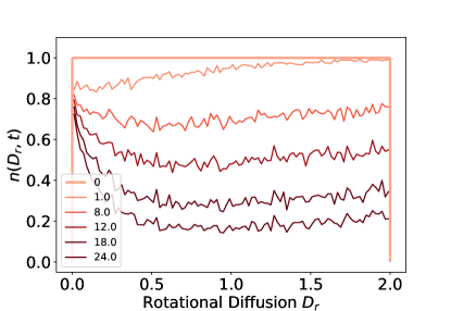
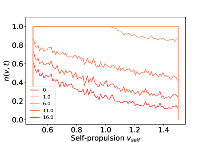
We are interested in the time evolution of the number of particles with velocity $v$ that falls into the interval $v\in[v,v+dv]$, with $dv=(v_{max}-v_{min})/\mathcal{N}$, with $\mathcal{N}=100$.

In Fig. (4) the time-evolution of $n(v,t)$ is shown as a function of $v$ for $5$ time steps. Dashed red curve indicates the initial uniform configuration. The second distribution is taken at $t=1$, as soon as the first particles have found the exit. As one can see, the only particles escaped are those with $v_{self}>v_{self}^{*}$. With increasing time, also particles with $v_{self}<v_{self}^{*}$ start to escape from the chamber, with times that depend upon $v_{self}$.

An alternative - and informative - way of seeing these results is studying the relaxation dynamics towards zero of $n(v,t)$ as a function of time. We recall that $n(v,t)$ at a given $v=v_{self}$ is the survival probability in this problem, which is the complementary cumulative of the probability density function $p(v,s)$ of having first exit at time $s$:

$$n(v,t)=\int_{t}^{\infty}dsp(v,s),$$ (6)

or equivalently

$$p(v,s)=-\frac{dn(v,t)}{dt}.$$ (7)

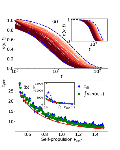
The results are reported in Fig. (5). In panel (a), $n(v,t)$ is shown for different values of self-propulsion velocities, increasing from light to dark red. We notice that a simple exponential relaxation characterized by a single velocity-dependent time-scale $\tau(v)$ might capture the behavior of $n(v,t)$ as a function of time. We show the results of exponential fits of the decay $n_{fit}(v,t)=A\exp{(-t/\tau_{fit}(v))}$, with $A\sim 1$. Dashed blue curve in panel (a) are two representative fits for $v_{min}=0.5$ and $v_{max}=1.5$. In the inset of the same panel, the decay of $n(v,t)$ for a larger chamber is also reported, for comparison. In this case, we have increased the radius of the circular confinement of an order of magnitude, i. e., $R=10$, making the threshold velocity $v_{self}^{*}\approx 10$. All particles have now a persistence length much smaller than the size of the chamber and are in the diffusive regime, with slow escape.

Moreover, in view of Eq. (7), the knowledge of $n(v,t)$ gives us immediate access to the average mean first exit time:

$$\tau_{FPT}(v)=\int_{0}^{\infty}dssp(v,s)=\\ -\int_{0}^{\infty}ds\,s\frac{dn(v,s)}{ds}=\int_{0}^{\infty}{\color[rgb]{0,0,0}ds}\,n(v,s).$$ (8)

It is worth noting that, in the case of a purely exponential relaxation, i. e., $n(v,t)=e^{-t/\tau_{fit}(v)}$, $\tau_{FPT}(v)$ coincides with $\tau_{fit}$. The behavior of $\tau_{FPT}$ as a function of $v_{self}$ is shown in panel (b). As one can appreciate, $\tau_{FPT}$ and $\tau_{fit}$ are in a nice agreement for $R=1$. The solid curve is Eq. (5) with the values of the parameters $\alpha$ and $\beta$ previously fitted. In the experiment with $R=1$ (main plot) the crossover can be appreciated from small to large velocities where $\tau_{fit}$ decays and then reaches a plateau. When $R=10$, on the contrary, the plateau is not reached and the $1/v_{self}^{2}$ scaling can be appreciated, see Eq. (5).

Figure 7: Decay of the number density for different $D_{r}$. Time evolution of $n(D_{r},t)$, the rotational diffusion $D_{r}$ decreases from $2$ (dark red) to $0$ (light red). The inset shows the decay time $\tau$ as a function of $D_{r}$. Solid red curve is $f(x)$ with $\alpha$ and $\beta$ previously fitted from $\tau_{FPT}$.

IV.2 Different persistence times

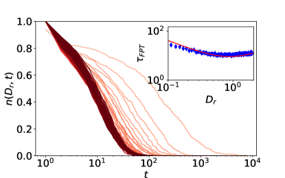
In this section we tune the persistence length $\ell$ by varying the persistence time $\tau_{pers}$ - which is $1/D_{r}$ for the case considered here of Active Brownian particles - and maintaining fixed the self-propulsion velocity $v_{self}$. We investigate the behavior of a sample composed by the same number of particles of the previous case with same self-propulsion velocity, i. e., $v_{self}=1$, and characterized by an initial distribution of rotational diffusion $\rho(D_{r})=\frac{1}{D_{r,max}-D_{r,min}}\left[\vartheta(D_{r}-D_{r,min})-\vartheta(D_{r}-D_{r,max})\right]$, with $D_{r,max}=2$ and $D_{r,min}=0$. The results are shown in Fig. (6). Note that, in this case, particles with $D_{r}=0$ remain trapped unless they starts with the right direction.

In Fig. (7) the typical behavior of $n(D_{r},t)$ as a function of time is shown. In this case we observe for the very low values of $D_{r}$ (high activity) that a single exponential decay does not reproduce the decay of $n(D_{r},t)$: interestingly, the survival probability seems to follow a first decrease to a plateau followed by a second final decay.

Again we measure $\tau_{FPT}$ from Eq. (8) and plot it in the inset of Fig. 7. According with the scaling of $\tau_{FPT}$ we discussed in section III, $\tau_{FPT}$ matches two asymptotic regimes, the first one, for small $D_{r}$ values and thus large persistence length, is $\tau_{FPT}\sim D_{r}^{-1}$. The second one is typical of the diffusive regime, meaning that $\tau_{FPT}\sim D_{r}$. In the inset of the same figure we report $\tau_{FPT}$ as a function of $D_{r}$, with superimposed Eq. (5).

Figure 8: Sorting of Run-and-Tumble particles. (a) Time evolution of $n(v,t)$ as a function of $t$ with $v\in[0.5,1]$. The inset show the behavior of $\tau$. The dashed red curve is $f(x)$. (b) Time evolution of $n(\lambda,t)$ as a function of $t$ with $\lambda\in[0,2]$. In the inset we report $\tau$ as a function $\lambda$.

IV.3 Behavior of Run-and-Tumble particles

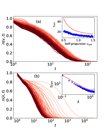
While the results in the previous sections have been obtained for Active Brownian particles, we have performed the same numerical simulations in the case of Run-and-Tumble dynamics, again for mixtures of particles with different propulsion velocities $v_{self}\in[0.5,1.5]$ and persistence times $\tau_{pers}=1/\lambda$ with $\lambda\in[0.01,2]$. The results, shown in Fig. (8) (a) and (b) respectively, are qualitatively the same of the previous cases: the relaxation dynamics of $n(v,t)$ and $n(\lambda,t)$ are well described by an exponential decay, unless the persistence time is very large ($\lambda\ll 1$). We notice that the non-exponential decay occurs for a larger range of persistence time with respect to the Active Brownian case (compare Fig. 7-(b) and Fig. 6): in our opinion this observation corroborates a correlation between the two-steps decay and ballistic behavior, which suggests that typical exit trajectories at large $\tau_{pers}$ are composed of two separate processes: first, the particle reach the boundary and second the particles finds the exit remaining close to the boundary . The behavior of $\tau_{FPT}$ is also reported in the insets of the two plots in Fig. (8).

V Discussion and Conclusions

In this work we have proposed a numerical study of the narrow escape problem of active particles in circular domains. We compared two paradigmatic models of active motions that are Active Brownian dynamics Bialké et al. (2015), suitable for reproducing the trajectories of smooth swimmers, and Run-and-Tumble dynamics, that, for instance, well captures the morphological properties of E. coli trajectories Berg (2008). We showed that in both dynamics $\tau_{FPT}$ turns to be bounded by two limiting asymptotic regimes. The two regimes result from the competition between the two characteristic length of the system: the persistence length $\ell$ and the radius $R$ of the container. When the persistence length is much smaller than the radius, i. e., $\ell/R\ll 1$, the active particles behaves as a Brownian random walker and $\tau_{FPT}$ diverges as the effective diffusivity of the random walk goes to zero. In the opposite limit, the persistence length is much larger than the size of the chamber, i. e., $\ell/R\gg 1$. The escaping dynamics is thus dominated by the ballistic regime and $\tau_{FPT}$ grows linearly with $\tau_{pers}$. We have introduced an empirical scaling function $f(x)$, with $x=\ell^{2}R^{-2}$, that smoothly connects these two asymptotic regimes.

We thus explored the possibility to take advantage of the crossover in the escape time between the active and the diffusive regime for sorting particles of different velocities. We obtained that, considering a gas of Active Brownian particles of different velocities and same rotational diffusion constant, by tuning the size of the chamber faster particles can be separated by the others. The same technique can be employed for demixing particles of different rotational diffusion. We showed that the same is true also in the case of Run-and-Tumble dynamics.

It is worth noting that the sorting mechanism explored here is dynamical and it works only on a finite time scale. In particular, waiting sufficiently long time, all particles escaped from the confining structure. However, in practical situation, the typical experimental time scale can be tuned for sorting microswimmers of different velocities tuning just the typical size of the confining structures, i. e., without introducing any external potential or complicated microsctructure. This could be useful in assistant reproductive technologies, where the challenge consists in maximize motile sperm concentration, sperm volume and lifetime. Usually, sperms are selected based on their motility. Our findings suggests that it could be done without introducing density gradient centrifugation Nosrati et al. (2017); Koh et al. (2015).

References

- Bechinger et al. (2016) C. Bechinger, R. Di Leonardo, H. Löwen, C. Reichhardt, G. Volpe, and G. Volpe, Rev. Mod. Phys. 88, 045006 (2016), URL https://link.aps.org/doi/10.1103/RevModPhys.88.045006.
- Marchetti et al. (2013) M. C. Marchetti, J. F. Joanny, S. Ramaswamy, T. B. Liverpool, J. Prost, M. Rao, and R. A. Simha, Rev. Mod. Phys. 85, 1143 (2013), URL https://link.aps.org/doi/10.1103/RevModPhys.85.1143.
- Maggi et al. (2017) C. Maggi, M. Paoluzzi, L. Angelani, and R. Di Leonardo, Scientific reports 7, 17588 (2017).
- Zhang et al. (2010) H.-P. Zhang, A. Be’er, E.-L. Florin, and H. L. Swinney, Proceedings of the National Academy of Sciences 107, 13626 (2010).
- Lushi et al. (2014) E. Lushi, H. Wioland, and R. E. Goldstein, Proceedings of the National Academy of Sciences 111, 9733 (2014).
- Bricard et al. (2013) A. Bricard, J.-B. Caussin, N. Desreumaux, O. Dauchot, and D. Bartolo, Nature 503, 95 (2013).
- Sanchez et al. (2012) T. Sanchez, D. T. Chen, S. J. DeCamp, M. Heymann, and Z. Dogic, Nature 491, 431 (2012).
- Angelani et al. (2009) L. Angelani, R. Di Leonardo, and G. Ruocco, Physical review letters 102, 048104 (2009).
- Di Leonardo et al. (2010) R. Di Leonardo, L. Angelani, D. Dell’Arciprete, G. Ruocco, V. Iebba, S. Schippa, M. Conte, F. Mecarini, F. De Angelis, and E. Di Fabrizio, Proceedings of the National Academy of Sciences 107, 9541 (2010).
- Sokolov et al. (2010) A. Sokolov, M. M. Apodaca, B. A. Grzybowski, and I. S. Aranson, Proceedings of the National Academy of Sciences 107, 969 (2010).
- Maggi et al. (2016) C. Maggi, J. Simmchen, F. Saglimbeni, J. Katuri, M. Dipalo, F. De Angelis, S. Sanchez, and R. Di Leonardo, Small 12, 446 (2016).
- Galajda et al. (2007) P. Galajda, J. Keymer, P. Chaikin, and R. Austin, Journal of bacteriology 189, 8704 (2007).
- Angelani et al. (2011) L. Angelani, A. Costanzo, and R. Di Leonardo, EPL (Europhysics Letters) 96, 68002 (2011).
- Reichhardt and Reichhardt (2017) C. O. Reichhardt and C. Reichhardt, Annual Review of Condensed Matter Physics 8, 51 (2017).
- Schnitzer (1993) M. J. Schnitzer, Physical Review E 48, 2553 (1993).
- Vladescu et al. (2014) I. D. Vladescu, E. J. Marsden, J. Schwarz-Linek, V. A. Martinez, J. Arlt, A. N. Morozov, D. Marenduzzo, M. E. Cates, and W. C. K. Poon, Phys. Rev. Lett. 113, 268101 (2014), URL https://link.aps.org/doi/10.1103/PhysRevLett.113.268101.
- Das et al. (2018) S. Das, G. Gompper, and R. G. Winkler, New Journal of Physics 20, 015001 (2018).
- Mijalkov and Volpe (2013) M. Mijalkov and G. Volpe, Soft Matter 9, 6376 (2013).
- Kaiser et al. (2012) A. Kaiser, H. H. Wensink, and H. Löwen, Phys. Rev. Lett. 108, 268307 (2012), URL https://link.aps.org/doi/10.1103/PhysRevLett.108.268307.
- Costanzo et al. (2014) A. Costanzo, J. Elgeti, T. Auth, G. Gompper, and M. Ripoll, EPL (Europhysics Letters) 107, 36003 (2014).
- Kumar et al. (2019) N. Kumar, R. K. Gupta, H. Soni, S. Ramaswamy, and A. K. Sood, Phys. Rev. E 99, 032605 (2019), URL https://link.aps.org/doi/10.1103/PhysRevE.99.032605.
- Nosrati et al. (2017) R. Nosrati, P. J. Graham, B. Zhang, J. Riordon, A. Lagunov, T. G. Hannam, C. Escobedo, K. Jarvi, and D. Sinton, Nature Reviews Urology 14, 707 (2017).
- Koh et al. (2015) J. B. Y. Koh et al., Microfluidics and Nanofluidics 18, 755 (2015).
- Gaffney et al. (2011) E. A. Gaffney, H. Gadêlha, D. Smith, J. Blake, and J. Kirkman-Brown, Annual Review of Fluid Mechanics 43, 501 (2011).
- Campana et al. (1996) A. Campana, D. Sakkas, A. Stalberg, P. G. Bianchi, I. Comte, T. Pache, and D. Walker, Human Reproduction 11, 732 (1996).
- Bénichou and Voituriez (2014) O. Bénichou and R. Voituriez, Physics Reports 539, 225 (2014).
- Singer et al. (2006a) A. Singer, Z. Schuss, and D. Holcman, Journal of statistical physics 122, 465 (2006a).
- Rupprecht et al. (2016) J.-F. m. c. Rupprecht, O. Bénichou, and R. Voituriez, Phys. Rev. E 94, 012117 (2016), URL https://link.aps.org/doi/10.1103/PhysRevE.94.012117.
- Paoluzzi et al. (2015) M. Paoluzzi, R. Di Leonardo, and L. Angelani, Phys. Rev. Lett. 115, 188303 (2015), URL https://link.aps.org/doi/10.1103/PhysRevLett.115.188303.
- Paoluzzi et al. (2014) M. Paoluzzi, R. Di Leonardo, and L. Angelani, Journal of Physics: Condensed Matter 26, 375101 (2014).
- Paoluzzi et al. (2013) M. Paoluzzi, R. Di Leonardo, and L. Angelani, Journal of Physics: Condensed Matter 25, 415102 (2013).
- Paoluzzi et al. (2018) M. Paoluzzi, M. Leoni, and M. C. Marchetti, Physical Review E 98, 052603 (2018).
- Kac (1974) M. Kac, The Rocky Mountain Journal of Mathematics 4, 497 (1974).
- Khatami et al. (2016) M. Khatami, K. Wolff, O. Pohl, M. R. Ejtehadi, and H. Stark, Scientific reports 6, 37670 (2016).
- Redner (2001) S. Redner, A guide to first-passage processes (Cambridge University Press, 2001).
- Singer et al. (2006b) A. Singer, Z. Schuss, D. Holcman, and R. S. Eisenberg, Journal of Statistical Physics 122, 437 (2006b).
- Rupprecht et al. (2015) J.-F. Rupprecht, O. Bénichou, D. Grebenkov, and R. Voituriez, Journal of Statistical Physics 158, 192 (2015).
- Angelani et al. (2014) L. Angelani, R. Di Leonardo, and M. Paoluzzi, The European Physical Journal E 37, 59 (2014).
- Angelani (2015) L. Angelani, Journal of Physics A: Mathematical and Theoretical 48, 495003 (2015).
- Bialké et al. (2015) J. Bialké, T. Speck, and H. Löwen, Journal of Non-Crystalline Solids 407, 367 (2015).
- Berg (2008) H. C. Berg, E. coli in Motion (Springer Science & Business Media, 2008).