Central velocity dispersion catalog of LAMOST-DR7 galaxies

Abstract

The Large Sky Area Multi-Object Fiber Spectroscopic Telescope (LAMOST) is a major facility to carry out spectroscopic surveys for cosmology and galaxy evolution studies. The seventh data release of the LAMOST ExtraGAlactic Survey (LEGAS) is currently available and including redshifts of 193 361 galaxies. These sources are spread over $\sim 11\,500$ deg² of the sky, largely overlapping with other imaging (SDSS, HSC) and spectroscopic (BOSS) surveys. The estimated depth of the galaxy sample, $r\sim 17.8$, the high signal-to-noise ratio, and the spectral resolution $R=1800$, make the LAMOST spectra suitable for galaxy velocity dispersion measurements, which are invaluable to study the structure and formation of galaxies and to determine their central dark matter (DM) content. We present the first estimates of central velocity dispersion of $\sim 86\,000$ galaxies in LAMOST footprint. We have used a wrap-up procedure to perform the spectral fitting using pPXF, and derive velocity dispersion measurements. Statistical errors are also assessed by comparing LAMOST velocity dispersion estimates with the ones of SDSS and BOSS over a common sample of $\sim 51\,000$ galaxies. The two datasets show a good agreement, within the statistical errors, in particular when velocity dispersion values are corrected to 1 effective radius aperture. We also present a preliminary Mass-$\sigma$ relation and find consistency with previous analyses based on local galaxy samples. These first results suggest that LAMOST spectra are suitable for galaxy velocity dispersion measurements to complement the available catalogs of galaxy internal kinematics in the northern hemisphere. We plan to expand this analysis to next LAMOST data releases.

1 INTRODUCTION

Spectroscopic surveys are fundamental tools to determine galaxy distances through their redshifts and map their distribution across time and space, e.g. to reconstruct their large scale structure (see e.g., the 2dF Galaxy Redshift Survey, 2dFGRS, Colless et al. 2001; the 6dF Galaxy Redshift Survey, 6dFGRS, Jones et al. 2009; the Baryon Oscillation Spectroscopic Survey, BOSS, Dawson et al. 2013; the VIMOS Public Extragalactic Redshift Survey, VIPERS, Guzzo & Vipers Team 2017) and investigate their assembly (e.g. the Galaxy Mass Assembly, GAMA, Liske et al. 2015) and the evolution of their properties and clustering up to high redshift (e.g. the DEEP2 survey, Newman et al. 2013). Additionally, they are also used to calibrate the tools to derive photometric redshifts (see e.g., Cavuoti et al., 2015, 2017), which are invaluable for imaging surveys devoted to cosmological studies, making use, e.g., of weak gravitational lensing (e.g., Hildebrandt et al. 2017), baryonic acoustic oscillation (e.g., Ahn et al. 2012; Bautista et al. 2018) or large scale structure (e.g., Alpaslan et al. 2015).

Spectroscopic redshifts are also crucial for galaxy formation studies as they allow to accurately select galaxies at different cosmic epochs to study the main scaling relations such as size-luminosity and size-mass (Shen et al., 2003; Hyde & Bernardi, 2009a), Kormendy relation (KR, Kormendy, 1977; Hamabe & Kormendy, 1987), and trace these relations back in time (see e.g., Huertas-Company et al., 2013; Roy et al., 2018).

Besides galaxy redshifts, spectroscopic surveys can also provide galaxy kinematics (see e.g. Thomas et al. 2013), hence allowing to investigate more fundamental scaling relations like the Faber-Jackson and the mass–dispersion relation (Hyde & Bernardi 2009a), and the fundamental plane (e.g., La Barbera et al. 2010), investigating the correlation between central DM fraction, mass density slope, Initial Mass Function (IMF) and mass (Cappellari et al. 2006, 2013b; Tortora et al. 2009, 2012a, 2013; Tortora et al. 2014b, c, 2018a; Napolitano et al. 2010; Cardone & Tortora 2010; Thomas et al. 2009, 2011; Dutton & Treu 2014) and trace them back in time (see e.g., Tortora et al., 2010b; Tortora et al., 2018a; Beifiori et al., 2014) or probe alternative gravities (Tortora et al. 2014a, 2018b).

Figure 1: Sky distribution (RA, DEC) of LAMOST galaxy targets from the LEGAS survey. In red all sources labeled as galaxies, in blue the ones that have passed the SNR criteria (i.e. $SNR>10$ in $g$- or $i$-band) and in green the galaxies with measured velocity dispersion in this work.

These studies are especially valuable if one can combine internal kinematics with high image quality data, to determine accurate light profile of galaxies to be used to derive their central dynamics (see e.g. Beifiori et al. 2014; Tortora et al. 2018a), to study the galaxy-black hole co-evolution (e.g. Salviander & Shields 2013), and to combine the gravitational lensing with the internal kinematics of the lens to obtain constraints on the dark matter properties (e.g., Cardone et al. 2009; Cardone & Tortora 2010; Auger et al. 2010b; Tortora et al. 2010b) and the galaxy Initial Mass Function (e.g. Auger et al. 2010a; Sonnenfeld et al. 2015; Spiniello et al. 2015).

The accumulation of larger area of the sky with such a high-quality imaging data, both in Northern sky, e.g. with the Hyper Suprime-Cam Subaru Strategic Program (HSC, Miyazaki et al. 2012; Aihara et al. 2018), and in the Southern hemisphere, e.g. with the Kilo Degree Survey, KiDS and its twin near infrared VIKING survey (see e.g. Kuijken et al. 2019), or the Dark Energy Survey (DES, The Dark Energy Survey Collaboration, 2005), is making particularly useful to catch up with equally extended and possibly deep spectroscopic datasets from which galaxy kinematics can be extracted. For this reason, future surveys are specifically designed to cover this gap (e.g., WAVES@4MOST, Driver et al. 2016, STEPS/WEAVE@WHT Costantin et al. 2019).

The Large sky Area Multi-Object Fiber Spectroscopic Telescope (LAMOST) is a 4m effective aperture (6.67m main mirror sized) telescope located at the Xinglong Observatory northeast of Beijing, China (Wang et al. 1996; Cui et al. 2012; Zhao et al. 2012). The telescope is characterized by a $\sim 20$deg² field of view (FOV) where a total of 4000 circular fibers of 3.3 arcsec diameter can be mounted on its focal plane (Deng et al. 2012). With the capability of its large field of view and strong multiplexing ability, the LAMOST telescope is dedicated to a spectral survey of celestial objects over the entire available northern sky. LAMOST is a Chinese national scientific research facility operated by National Astronomical Observatories, Chinese Academy of Sciences (NAOC). Since the commissioning year started in 2009, LAMOST has carried out a spectral survey of millions of objects in a large part of the northern sky. The survey has two major components: the LAMOST ExtraGAlactic Survey (LEGAS) and the LAMOST Experiment for Galactic Understanding and Exploration (LEGUE).

Currently the survey has collected observations for one year pilot survey followed by eight year regular survey, and the seventh data release (DR7 hereafter) has been domestically delivered including the data of the first 7 years of regular survey plus the pilot survey.

In particular, the extragalactic component (LEGAS), has collected spectra for 193 361 galaxies and 64 236 quasars (see also §2.1). Like previous data releases, for all these sources data LAMOST-DR7 provides flux- and wavelength-calibrated, sky-subtracted spectra and a series of basic spectro-photometric information like right ascension, declination, signal-to-noise ratio (SNR hereafter), magnitude, source classification and redshift (see e.g. Luo et al. 2015).

These data have been already used for extragalactic science like the study of E+A galaxies (Yang et al. 2015), the analysis of quasar properties (Ai et al. 2016; Shi et al. 2014b), the discovery and analysis of double peaked AGNs (Huang et al. 2014; Shi et al. 2014a, Wang et al. 2019), the study of Luminous Infrared Galaxies (Lam et al. 2015), the detection and analysis of galaxy pairs (Shen et al. 2016, Feng et al. 2019), the study of compact groups (Zheng & Shen 2020), the spectral classification and composites of galaxies (Wang et al. 2018). Within the extragalactic program there is also the LAMOST Complete Spectroscopic Survey of Pointing Area (LaCoSSPAr) in the Southern Galactic Cap (Yang et al. 2018, Zhao et al. 2019), which is the only area (two fields of 20 deg² each) with a magnitude limited sample ($r=18.1$).

Deriving the velocity dispersion for a large subsample of LAMOST galaxies would represent a big scientific value, for instance: 1) to correlate the galaxy properties (e.g. luminosity, mass-to-light ratios, sizes, star formation rate) with a proxy of the halo mass, the velocity dispersion (e.g., Hyde & Bernardi 2009b, a), 2) to estimate DM fraction, mass density slope and IMF and their evolution with redshift (see e.g., Cappellari et al., 2006, 2013b; Tortora et al., 2009, 2013; Tortora et al., 2014b, 2018a; Beifiori et al., 2014); 3) to provide further and independent constraints on the total mass within the Einstein radius in strong-lensed systems (Cardone & Tortora 2010; Tortora et al. 2010b; Sonnenfeld et al. 2015), 4) to test DM models or alternative gravities (e.g., Tortora et al. 2014a, 2018b) 5) to discover compact and massive galaxies, which are expected to have large velocity dispersions (Saulder et al. 2015), avoiding the systematics in the galaxy size measurement, induced by the low spatial resolution of wide-field ground-based surveys (e.g., Tortora et al. 2018c).

In this work, we present the first catalog of galaxy central velocity dispersion (VD hereafter) measurements from spectra of galaxies in the LAMOST-DR7. For all calculations, we assume a cosmology with ($\Omega_{M}$, $\Omega_{\Lambda}$, $h$)=(0.3, 0.7, 0.7).

In §2 we briefly describe the LAMOST spectroscopic database used and the selections made to perform the VD measurements; in §3 we briefly illustrate the wrap-up procedure to perform the spectral fitting to derive the galaxy internal kinematics and introduce the the first LAMOST velocity dispersion catalog; in §3.2 we compare the LAMOST velocity dispersion estimates with the Sload Digital Sky Survey (SDSS) and BOSS and discuss the relative scatter. In §5 we introduce a preliminary analysis of the Mass-$\sigma$ relation using LAMOST galaxies for which we have found mass estimates from litarature. Finally, we discuss some perspective on the application of our procedure to next LAMOST data releases and draw some conclusions on §6

2 The spectroscopic data

2.1 The LAMOST ExtraGAlactic Survey

The LAMOST ExtraGAlactic Survey (LEGAS) is the key project in the LAMOST extragalactic mission. It is divided into two large patches in the northern galactic cap (NGC) and the southern galactic cap (SGC) and it targets pre-selected galaxies and QSOs. The NGC patch covers about 8000 deg² and has the same footprint as the SDSS Legacy Survey. It is aimed at observing SDSS galaxies (with $r\leq$ 17.8) that were not spectroscopic followed-up to avoid fiber collisions (Stoughton et al. 2002). The SGC patch covers about 3500 deg². In this latter region ($b$ < -30^∘ and $\delta$ > -10^∘ in a strip of equatorial coordinates 45${}^{\circ}<$ RA$<60^{\circ}$ and 0.5${}^{\circ}<$ DEC $<9.5^{\circ}$) LAMOST aims at taking spectra of galaxies with limiting magnitude $r<18$, and a sample of blue galaxies down to $r<18.8$. Besides these two well-defined samples of galaxies, some bright-infrared galaxies are chosen as extra observational targets that are selected from infrared surveys such as IRAS, WISE, and Herschel.

So far, the LAMOST consortium has delivered 7 public data releases, the last one, DR7, in March 2020. LAMOST-DR7 includes all targets delivered in previous releases, thus we will analyse 193 361 spectra classified as galaxies in the LAMOST catalog. We remark that this spectra database contains a number of re-visits, hence the actual number of observed galaxies is 163 765. We will retain the repeated spectra to evaluate the internal consistency of the fitting procedure and/or pick the highest quality among the repeated measurements (see 3.2.2).

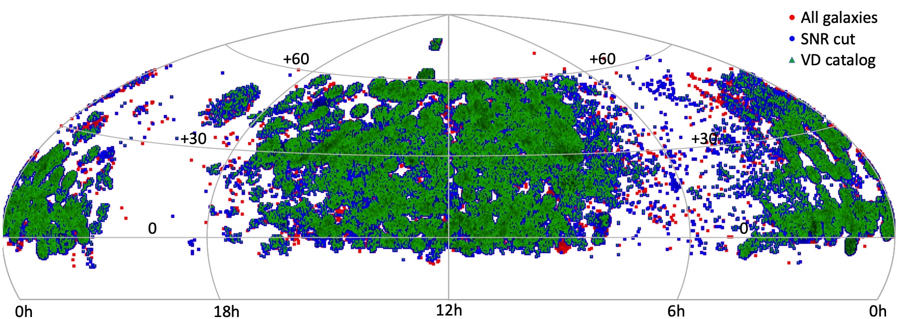
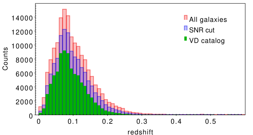
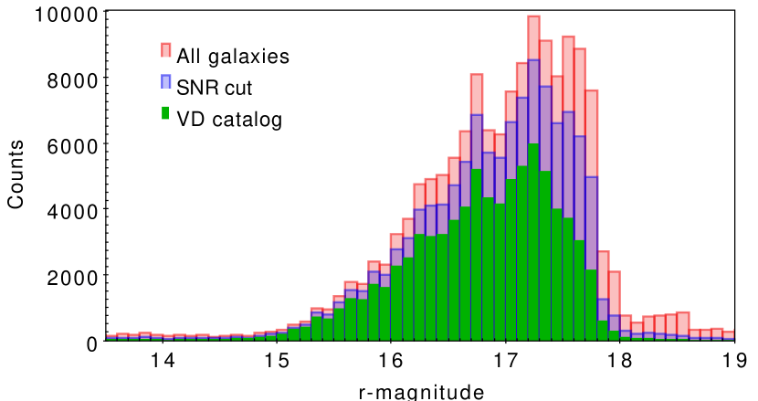
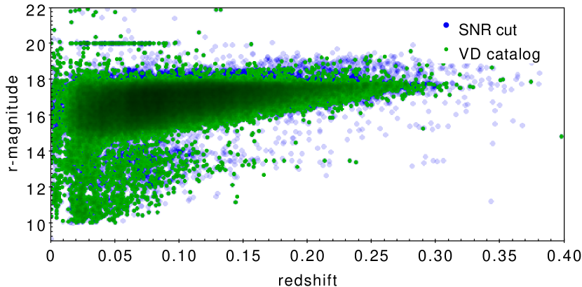
The sky distribution of the LAMOST-DR7 galaxies is shown in Fig. 1. Here we plot: 1) all galaxies currently available in the LAMOST database (in red), 2) the ones with high signal-to-noise ratio (in blue, see §2.2), and 3) the galaxies for which we have obtained VD measurements (in green, see §3). As mentioned in §1, the LaMOST-DR7 provides basic information for each galaxy in the catalog, including position, magnitude in 5 optical bands ($ugriz$), spectral SNR in the same bands, and the redshift with error derived by the LAMOST spectra (see Luo et al. 2015). In Fig. 2 we show the distribution of redshift, $z$  and $r-$band magnitude, $mag_{r}$, for the three galaxy subsets introduced above. In particular, LAMOST galaxies are mainly concentrated in the redshift range $z=$[0,0.3] and they have a mean redshift $\langle z\rangle=0.10\pm 0.06$ (where the error is the 1$\sigma$ scatter of the sample distribution). The $r-$band magnitude distribution mainly covers the range $mag_{r}=$[14.0,19.0] with a mean $\langle mag_{r}\rangle=17.0\pm 0.8$, and starts to become highly incomplete for $mag_{r}>17.8$, due to the adopted selection function (see above), although the higher SNR sample show a slightly brighter limiting magnitude (see 2.2).

Figure 2: Redshift (top) and $r-$band magnitude (bottom) distributions of LAMOST galaxies from the LEGAS survey. In red all sources labeled as galaxies, in blue the ones that have passed the SNR criteria (i.e. $SNR>10$ in $g$- or $i$-band) and in green the galaxies with measured velocity dispersion in this work. Note that both redshift and magnitude distributions have long tails that have been cut in the figures for graphical reasons.

2.2 LAMOST spectra

The LAMOST designed wavelength coverage is 3650-9000 Å and the resolution is $R\sim 1800$ increased from $R\sim 1000$ through narrowing the slit at the output end of the fibers to 2/3 the fiber for all 16 LAMOST spectrographs (see Luo et al. 2015).

On the original CCD image, 4K pixels are used for recording blue or red wavelength regions ranging from 3700 Å to 5900 Å or from 5700 Å to 9000 Å respectively. When the blue and red channels are combined together, each spectrum is re-binned to a resolution element of 69 km s^-1, which means the difference in wavelength between two adjacent points is $\log(\lambda)=0.0001$. Conventionally this resolution element is referred to as a “pixel” for LAMOST data (see also Luo et al. 2015 for further details).

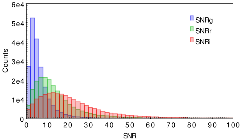
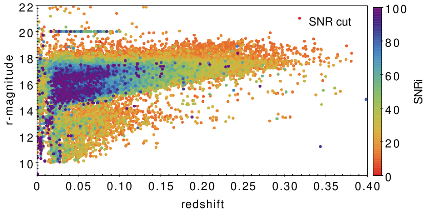
The SNR is defined per ‘pixel’ and calculated by using the inverse-variance, which is included in the spectral FITS files, in different band passes ($u,~{}g,~{}r,~{}i,~{}z$). The SNR for each pixel is given by the product between the flux and its inverse-variance (Luo et al. 2015). The mean SNR in a wavelength band can be averaged from the SNR of each pixel in the bandpass range. Another way to obtain SNR is to calculate the ratio between the continuum and the 1$\sigma$ (standard deviation) of the continuum noise. These two definitions of SNR are given in the LAMOST catalogs to provide a quality flag for LAMOST data (see Fig. 3), while they do not reflect the local SNR of the spectral features that are used to perform the velocity dispersion measurements. This latter SNR will be determined by the fitting procedure and used as a further quality criterion (see §3). According to the data release documentation (see Luo et al. 2015) a successful observational target with optimal data quality is defined if the “global” SNR$>10$ in $g$- or $i$-band. In the following we will adopt the same definition, although we plan to investigate less stringent constraints in future analyses. As it can be seen in Fig. 3, this condition is realised in $i-$band for the majority of spectra, while there is a shorter tail of galaxies with $g$-band, so the $i-$band SNR will be one mostly qualifying spectra for VD measurements. We will discuss all selection criteria of the LAMOST spectra in more details in the next section and the sample with measured VDs in §3.

2.3 Spectra selection for kinematic measurements

Since we are interested in extracting the galaxy VD from LAMOST spectra, the main criteria to select high-quality spectra is the SNR. As anticipated, we have followed the prescription from the LAMOST data releases and used as first criteria the $SNR>10$ in $g$- or $i$-band. The LAMOST pipeline also provides the keyword FIBERMASK, which reports possible problems of the fiber: this is an integer value which is $0$ for fibers with no problem and larger than 0 for fibers with issues (not allotted fiber, bad centering, the too low flux in sky flat frames, bad arc solution, $>10\%$ pixels are bad on CCD, $>10$ pixels are saturated, whopping fiber, near a whopping fiber, extreme residuals). As we will discuss in §3, the pipeline used to measure VDs will also perform an independent assessment of the spectra quality, focused on the fitted wavelength window.

Finally, the robustness of the VD estimates will also be checked against literature velocity dispersions from SDSS-Data Release 7 (SDSS-DR7 in short) and BOSS which have galaxies in common with LEGAS.

Figure 3: Signal to noise ratio distribution. The SNR/pixel as from the LAMOST galaxy catalog in $g-$band (blue), $r-$band (green) and $i-$band (red).

After the aforementioned SNR cut, we ended up with a list of a collection of 148 440 spectra, corresponding to 124 214 galaxies, which have been plotted on the sky in Fig. 1 and characterized in terms of their redshift and r-band magnitude distributions in Fig. 2 (blue colors).

However, all the criteria above do not guarantee that the spectra are suitable for the fitting procedure we want to perform, being the ratio of bad pixels/good pixels (on the main features considered for the spectrum fitting) the ultimate factor to assess the quality of the spectrum, which will be illustrated later (see §2.3). For this reason, after the criteria above have been used to preliminary select the spectra to be used for the fitting procedure, a further automatic selection is applied, which directly scans the spectra pixel by pixel to qualify them for the analysis.

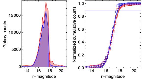
We can now give a more quantitative estimate of the relative completeness as a function of the magnitude of the galaxy sample before and after the SNR cut. This is obtained by fitting the normalized cumulative counts of the two samples shown in Fig. 4 with a standard error function model (see e.g. Rykoff et al. 2015).

$${\rm comp}=(1/2)\left[Erf\left(\frac{m-m_{100}}{\sqrt{2w}}\right)\right],$$ (1)

where $m_{100}$ is the magnitude at which the completeness is 100%, and $w$ is the (Gaussian) width of the rollover. The normalized cumulative counts are obtained by the $r-$band magnitude distribution in Fig. 2 (bottom). The magnitude at which the sample is 90% complete with respect to the total sample has been extrapolated by the best fit function and turned out to be $mag_{r}=17.84\pm 0.04$ and $mag_{r}=17.64\pm 0.04$ (errors are nominal from the fit, see Fig. 4). These magnitudes give a reasonable measure of the completeness of the sample due to the LAMOST selection function that sharply selects galaxies around $m_{r}=18$.

Figure 4: Left: Luminosity distribution of all sources labeled as galaxies (red), and the ones that have passed the SNR criteria (blue). The LAMOST selection function sharply selects galaxies around $m_{r}=18$. Short vertical lines show the 90% relative completeness of the LAMOST sample (see right panel). Right: relative completeness of the LAMOST galaxies with respect to the total sample all sources labeled as galaxies (red squares) and the ones that have passed the SNR criteria (blue squares). The horizontal line show the 90% relative completeness of the LAMOST sample. Overplotted the best-fit error function as in Eq. 1, with the $\pm 1\sigma$ confidence curves from the best-fit parameters.

Figure 5: Left: $r-$band magnitude vs. redshift for the LAMOST galaxy spectra belonging to the sample selected for the velocity dispersion run through the SNR cut (blue) and the one for which we have obtained the velocity dispersion (green). Right: the qualified spectra for the velocity dispersion are color-coded according to their $i-$band SNR as indicative of their quality. This shows that the spectra SNR degrades mainly at magnitudes fainter than 18; however there are also a number of lower SNR at $mag_{r}<14$ and redshift $z>0.02$ that causes an incompleteness of the sample in this parameter space. Both panels include the galaxies with duplicated spectra.

3 Velocity Dispersion Measurements

As mentioned earlier the resolution of the LAMOST spectra $R\sim 1800$, together with a sufficient SNR of the main spectral features that can be used for galaxy kinematics (i.e., CaII-K, CaII-H, H$\delta$, G-band and Mg), can be used to obtain kinematic information of the central galactic regions. Given this multitude of spectral features covered in the wavelength range, one can expect to reduce the typical errors of dispersion measurements to a few tens of $\rm km\,s^{-1}$, provided that these spectral features have a sufficient SNR (Hopkins et al. 2013). Although internal kinematics of galaxies was not a main driver of the LEGAS survey, VDs represent a very valuable added value for galaxy formation and DM studies, hence LAMOST can complement the SDSS/BOSS and GAMA samples, at redshifts $z<0.3$ in the NGC, and provide wide coverage of galaxies in the SGC, where there is almost no similar data available (see Fig. 1).

3.1 Velocity dispersion pipeline

LAMOST spectra have been fitted using a fully automatic Python wrapper procedure which selects, prepares, and applies the Penalized Pixel-Fitting, pPXF, software (Cappellari 2017) , in order to optimise the best-fit of galaxy spectra in the rest frame wavelength range, i.e. 3700-9900 Å (see §2.2).

pPXF works in pixels space, after having logarithmically rebinned the wavelength of both the observed spectrum and template library spectra. The $\chi^{2}$ minimisation is performed by making use of the Levenberg-Marquardt method. In the pPXF set-up, we make use of additive polynomials in order to reduce template mismatch and correct for imperfect sky subtraction and scattered light.
Since pPXF works on restframed spectra, the set-up of the software is made particularly easy by knowledge of galaxy redshifts. In order to apply pPXF to a large sample as LAMOST, we need to pay attention to the spectra selection and pre-processing (see §3.1.1). A similar approach has been already applied to obtain galaxy internal kinematics from other instruments (see e.g. Tortora et al. 2018c; Scognamiglio et al. 2020).

In the following we will illustrate all the main steps of the pipeline and the fitting strategies.

3.1.1 Spectral range

The first step of our analysis has been to pre-process LAMOST spectra and obtain the most homogeneous set of spectra, thoroughly masked for bad features, and restframed. For this latter step, we can rely on robust redshift measurements from previous LAMOST releases and easily de-redshift the LAMOST spectra before applying pPXF. The “high-quality” LAMOST spectra (selected according to the criteria in §2.3) have been passed to the pipeline to be analysed. Given the $z-$distribution of LAMOST galaxies (mainly at $z<0.065$, see Fig. 2), we decided to restrict our analysis to the restframe wavelength range: 3800-6000 Å in order to include only relevant absorption lines such as CaII-K, CaII-H, G-band, Mgb, and NaD. The adoption of a restricted (albeit still large) wavelength range has also dictated to reduce the computing time, which is mandatory for large datasets to limit the analysis to a few days on a personal desktop/laptop. To do that we needed to rest-frame the spectra and trim them to match one of the two selected wavelength ranges.

3.1.2 Templates and rebinning

We used a selection of 40 MILES simple stellar population synthesis models (SSPs) from Vazdekis et al. (2010) as reference templates. The choice of a limited number of templates allowed us to reduce the computational time, without affecting the accuracy of the VD estimates (see Appendix A for a discussion). The selected SSPs have a unimodal IMF with logarithmic slope $\Gamma$=1.3, metallicity ranging between -1.71 and 0.22, and age ranging between 1 Gyr and 12 Gyr. Following the pPXF prescriptions, template spectra are re-binned at the same velocity sampling of the LAMOST spectra. Subsequently, the template spectra are convolved with a Gaussian profile at the same instrumental resolution of 2.4 Å (Xiang et al., 2015) after having corrected the FWHM by the galaxy redshift (i.e. FWHM_rest=FWHM${}_{obs}/(1+z)$, as prescribed by pPXF).

3.1.3 Pixel-masking

A pixel mask is needed to exclude outlying pixels and bad features from the fitting procedure. As a first step, the pipeline conservatively masks the wavelengths of typical gas emission lines, in order to avoid possible contamination by emission lines, like: H$\rm{\delta}$4101.74Å, H$\rm{\gamma}$4340.47Å, H$\rm{\beta}$4861.33Å, $\rm[OIII]$4958.92Å, $\rm[OIII]$5006.84Å. We have checked that this conservative masking does not affect the measurement.
In addition to this brute force masking of typical emission lines, pPXF performs a preliminary fit and we take advantage of a sigma-clipping cut at 3-$\sigma$ level of the remaining hot pixel. A spectrum having more than 50% of bad pixels is automatically discarded from the analysis.
Finally, all spectra which pass this quality assessment are restframed using the LAMOST catalogued redshifts and processed with pPXF, by making use of an additive polynomial of the 4-th degree and letting the program to fit only two moments of the LOSVD (i.e. assuming a Gaussian distribution). Beside the redshift used to restframe the spectra, we used a $\sigma_{\rm start}=200$ kms^-1 as initial condition for all galaxies in the pPXF run.

3.2 The LAMOST velocity dispersion catalog

In this section, we describe the further criteria we have adopted to obtain a catalog of reliable velocity dispersion estimates and evaluate some completeness magnitude. These include some criteria on the $\chi^{2}$ of the best-fit model of the spectra and a range of acceptable values for galaxy-like VDs. We also use the information from multiple spectra of the same source to map the internal errors of the method. Finally, we describe the content of the delivered catalog.

Figure 6: Left: statistical relative errors from repeated spectra of individual galaxies, $\delta\sigma/\sigma_{\rm mean}$ (blue dots, see text for a detailed description) and relative errors from pPXF (red dots) as a function of the $i-$band SNR as a proxy of the overal spectra SNR. Overplotted the shaded areas corresponding to a $\pm 1\sigma$ scatter around a running mean. Right: $\delta\sigma/\sigma_{\rm mean}$ as a function of the best-fit $\chi^{2}$. Here there is a clear linear correlation which is quantified by the linear fit overplotted to the individual galaxy values (blue dots). The shaded area show the $3\sigma$ confidence interval of the best-fit parameters.

3.2.1 $\chi^{2}$ and velocity dispersion cuts

The pPXF run has returned the velocity dispersion for all spectra fed in the pipeline (i.e. 148 440 entries). However, we have performed an a posteriori quality check based on three main criteria:

1. signal-to-the-residual ratio (SRR)>5;

2. $\chi^{2}_{\rm FIT}$ < 1.1;

3. 50 km/s $\leq\sigma_{\rm meas}\leq$ 450 km/s.

where SRR is the ratio between the median value of the flux and the rms of the residuals of the fit retrieved with pPXF, and $\chi^{2}_{\rm FIT}$ is the reduced $\chi^{2}$ of the pPXF fit measured on the considered wavelength range. The lower velocity dispersion limit is adopted to cut those galaxies with a measured sigma lower than 2/3 of the velocity scale of the instrument. By accepting these galaxies, we want to introduce in our final catalogue those measurements which are still higher than the MILES library resolution and which can be statistically significant for general purpose analyses without introducing biases due to a too stringent selection based on the sole velocity scale of the instrument. Similarly, we cut those galaxies with unrealistically high velocity dispersion ($>$450 km/s) considering the galaxy sample we are analysing

Using these criteria, we ended up with a sample of 98 340 galaxies with measured velocity dispersions. These become 99 515 if we use a looser cut on velocity dispersion of 35 km/s $<\sigma_{\rm meas}<$ 450 km/s.

To understand what are the galaxies missed after this last selection criteria, in Fig. 5 (left panel) we show the $r-$band magnitude of the galaxy samples fed into the velocity dispersion pipeline (i.e. that qualifies because of the SNR criteria) and that survived the cut above after the velocity dispersion measurements. In the same figure (right panel) we also show the ingested galaxies color-coded by their SNR in $i-$band (as a proxy of their quality). From these plots, it is evident that the galaxies with velocity measurements tend to occupy the regions of the plot with higher SNR. However, there is a region with lower SNR at $mag_{r}<14$ and redshift $z>0.02$ that produces a lower incompleteness of the velocity dispersion sample. From the figure, it is also trivially clear that the SNR increases at lower redshift and/or in the brightest galaxies.

3.2.2 Repeated spectra: realistic relative errors and duplication cleaning

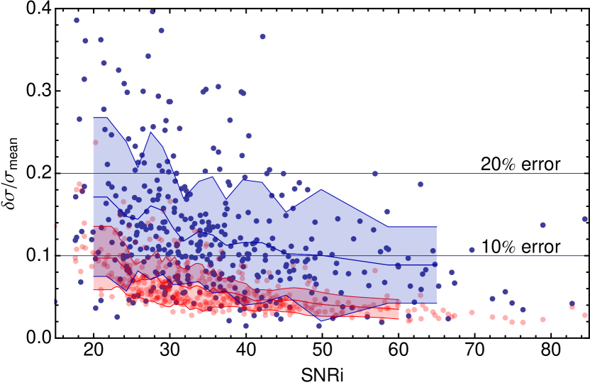
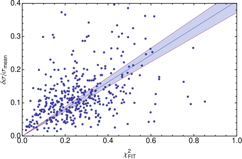
As mentioned earlier, the LAMOST database contains repeated spectra, i.e. multiple observations of the same sources. We have checked that in the sample of 98 340 spectra, which survived after the criteria applied in §3.2.1, there are 22 194 which are repeated spectra (from 2 to 22 re-visit) of 9 715 sources, while the remaining 76 146 have a single spectrum available. Obviously, we need to define the best velocity dispersion estimate for the repeated sources among the ones produced by our pipeline, and clean all the duplication from the final catalog. We will address this point at the end of this section. Before proceeding to that, we notice that the repeated velocity dispersion measurements from independent spectra can allow a direct and quantitative evaluation of the overall statistical uncertainties of the full pipeline, as this is applied to different spectra of the same galaxy with different properties like SNR, noise, calibration etc. To evaluate these statistical errors we have selected all galaxies with several spectra larger than 4 (a total of 402 systems) and estimated for them: 1) the mean VD ($\sigma_{\rm mean}$), 2) mean velocity dispersion errors, 3) mean $i-$band SNR, 4) mean $\chi^{2}_{\rm FIT}$ and their standard deviations. For each galaxy, we could define the statistical relative errors as $\delta\sigma/\sigma_{\rm mean}$, where $\delta\sigma$ is the standard deviation of the different spectra for the individual galaxy and $\sigma_{\rm mean}$ is defined as above. In Fig. 6 we show the relative VD errors as a function of the SNR in the mean $i-$band SNR and the mean $\chi^{2}_{\rm FIT}$ obtained from the same repeated spectra for each galaxy. First, we notice that the statistical relative errors are larger than the nominal ones that one would obtain from the errors given by the pPXF output. These latter are given in the same Fig. 6 (left panel) as red dots, which are obtained by the ratio of the mean VD errors from pPXF in the repeated estimates and $\sigma_{\rm mean}$. In particular, the mean relative errors are about half of the statistical relative errors at any given SNR value. Second, as expected the statistical relative errors (as well as the mean pPXF relative errors) are a decreasing function of the SNR and go from $0.16\pm 0.12$ at SNR${}_{i}=20$ to $0.10\pm 0.08$ at SNR${}_{i}=80$.

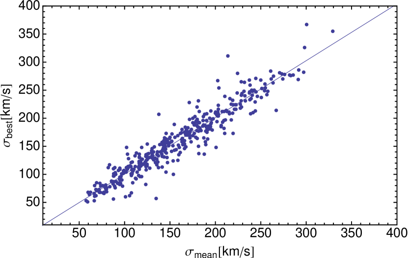
In the right panel of Fig. 6 we show the statistical $\delta\sigma/\sigma_{\rm mean}$ as a function of the $\chi^{2}$ from the pPXF to the full spectra. Here we see that there is a clear correlation between the relative errors and the quality of the overall fit, i.e. the lower the $\chi^{2}_{\rm FIT}$ the lower the $\delta\sigma/\sigma_{\rm mean}$. To quantify this we have: 1) estimated a Spearman’s rank correlation coefficient, $\rho=0.407\pm 0.004$ (where the error is the standard deviation over 1000 jackknife extractions of the 2 parameters randomly cutting 1% of the sample at every run), which corresponds to $>99\%$ correlation significance according to the Student’s t-distribution ($dof=$n. data$-$2=400); 2) performed the linear fit $y=Ax$ where $A=0.42\pm 0.02$ (hence significantly different from zero), which is also shown in the same panel with the shaded region corresponding to the $3\sigma$ confidence level. This tight correlation suggested us to use the lowest $\chi^{2}_{\rm FIT}$ to pick the best estimate, $\sigma_{\rm best}$, for each of the 9 715 galaxies with multiple measurements. In Fig. 7 we plot $\sigma_{\rm best}$ with the $\sigma_{\rm mean}$ for each of the 402 galaxies as in Fig. 6: they are perfectly on the one-to-one relationship with a very small scatter, defined as the standard deviation of the quantity $1-\sigma_{\rm mean}/\sigma_{\rm best}$), and found to be $\sim 0.12$, consistently with average statistical errors on Fig. 6 (left panel). This means that the $\sigma_{\rm best}$ is a good probe of the true velocity dispersion of these systems. We have then obtained the $\sigma_{\rm best}$ for all the galaxies with multiple spectra (9 715) which we added to the single spectra systems (76 146) to obtain a final catalog of 85 861. We summarize all the samples discussed in the last sections and relative numbers in Table 1.

	All	Galaxies	Repeated	Single
DR7 Spectra	193 883	163 765	53 128	140 775
SNR cut	148 440	127 093	36 348	112 092
VD catalog	98 340	85 861	22 194	76 146

Table 1: LAMOST VD Catalog Content. Reported the number of LAMOST spectra of the DR7 and the relative number of Galaxies, for the whole sample, the adopted SNR cut and the final catalog of VD measurements. Also reported the number of single and repeated spectra for each sample.

Figure 7: Mean VD from more than 4 repeated spectra, $\sigma_{\rm mean}$, vs. the best estimate, $\sigma_{\rm best}$, for each galaxy, given as the VD corresponding to the lowest $\chi^{2}_{\rm FIT}$ among the repeated measurements. Overplotted to the individual datapoints, the one-to-one line to show the perfect match between the two quantities.

Figure 8: The relative deviation of the LAMOST measured VDs from pPXF, $\sigma_{\rm FIT}$, and SDSS estimates, $\sigma_{\rm SDSS}$ (top), or BOSS, $\sigma_{\rm{BOSS}}$ (bottom), as a function of $n-$index (left panel) and effective radius equivalent parameter, sersic$-R_{50}$, (right panel). The red shaded regions show the 16% and 84% quantiles, while the central solid line shows the median of the $(\sigma_{\rm FIT}-\sigma_{\rm SDSS})/\sigma_{\rm FIT}$ distribution in both panels.

3.2.3 Final catalog content

We release the catalog of the sample of 85 861 galaxies as an added value dataset of the LAMOST-DR7 data release. This is a first version of the velocity dispersion catalog that we plan to refine in future releases by: 1) a more accurate cleaning of the spectra quality throughout a more systematic triage based on spectra inspection (e.g. using machine learning techniques to assess the spectra quality); 2) bootstrapping the results by changing the pPXF setup and 3) randomly resampling the spectra (see Appendix A for more details).

For this first LAMOST-DR7 catalog we report the following information:

• specid, the unique LAMOST spectrum ID;

• ra, right ascension (J2000) of the spectrum;

• dec, declination (J2000) of the spectrum;

• z, the redshift already measured by LAMOST pipeline;

• $\Delta z$, the redshift offset between LAMOST and pPXF derived measurement (see below);

• $\Delta z\_err$, the redshift offset error;

• veldisp, the velocity dispersion;

• veldisp_err, the velocity dispersion error;

• sng, the LAMOST released $g-$band SNR;

• snr, the LAMOST released $r-$band SNR;

• sni, the LAMOST released $i-$band SNR;

• srr_fit, the a posteriori measured SRR on the fitted wavelength window;

• chi2_fit, the $\chi^{2}/DOF$ measured on the fitted wavelength window.

The offset in redshift measurements $\Delta z$ arises from the fact that pPXF just refines, by matching the best linear combination of templates with the observed spectrum, the radial velocity starting from an initial redshift guess (which in our case is the one measured by LAMOST by making use of PCA methods, Yang et al. 2018). The mean offset between the pPXF redshift measurements and the ones released by LAMOST is $10^{-4}$ and the mean error $\Delta z_{\rm err}$, arising from the combination of the two measurement errors, is $10^{-3}$. One reason for the offset is the different wavelength range adopted by the VD pipeline, while LAMOST pipeline uses all wavelength range (see Du et al. 2019, for a detailed discussion).

Figure 9: The relative deviation of the LAMOST measured VD from pPXF, $\sigma_{\rm FIT}$, and SDSS estimates, $\sigma_{\rm SDSS}$, from NYU-VAGC (Blanton et al. 2005) as a function of $\sigma_{\rm FIT}$ (left column) and the SNR in $i-$band (right column), for the original fiber aperture spectra (top row, in blue/red) and the aperture corrected VD values (bottom row, in purple, together with the corresponding uncorrected values as comparison). All shaded regions show the 16% and 84% quantiles, while the central solid line shows the median of the $(\sigma_{\rm FIT}-\sigma_{\rm SDSS})/\sigma_{\rm FIT}$ distribution.

4 Comparison with SDSS and BOSS

We can now check the new LEGAS galaxy VD estimates against external catalogs of VDs measured on LEGAS targets. As discussed in §2.1, LEGAS has a large overlap with SDSS (DR7) and BOSS (SDSS-DR12) in the NGC, and we can compare VD measurements on common objects. For the SGC, most of the information about LEGAS targets comes from the Panoramic Survey Telescope and Rapid Response System (Pan-STARRS, Chambers et al. 2016) and no structural parameters, nor stellar masses have been associated with LEGAS galaxies.

4.1 Comparison of the nominal estimates from fiber spectra

For SDSS we use the NYU-VAGC (Blanton et al. 2005) as a reference catalog as this provides additional photometric information, like the effective radius ($R_{e}$), the Sérsic index ($n-$index, Sersic 1968) and the total Petrosian magnitude. In particular, since the $n-$index is distributed almost uniformly over the range of [0-6], i.e. LAMOST galaxies encompasses a wide range of galaxy types, we can test the consistency of the LAMOST estimates against SDSS as a function of the galaxy structural parameters. In general, to fairly compare independent measurements one should scale them at the same physical scale, e.g. the effective radius or some standard fraction of it (e.g. $R_{e}/8$, like usually used for fundamental plane analyses, see e.g. ref.). However, the difference between the LAMOST and SDSS fiber sizes is rather small, $R_{\rm Ap,lamost}=3.3^{\prime\prime}$ vs. $R_{\rm Ap,sdss}=3.0^{\prime\prime}$, so we expect this to have a minor impact on the measured kinematics from the spectra (see below).

The match of the LAMOST VD catalog (85 861 entries) with the NYU-VAGC (2 506 754 entries) returned 66 045 objects, although a quite significant number of the matched sources from SDSS have a VD=0 and cannot be used for our comparison. The final catalog with suitable VDs from SDSS is made of 50 533 entries: we will refer to this as the LAMOST_SDSS_VD_SERSIC catalog, to indicate that for these systems we have both internal kinematics and Sersic structural parameters from SDSS.

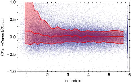
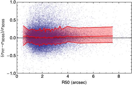
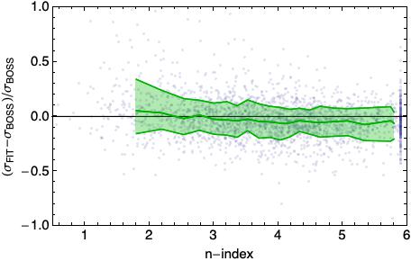
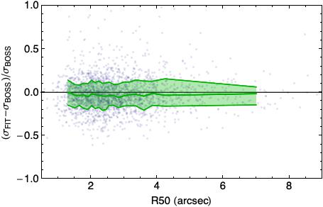
In Fig. 8 we plot the relative deviation of the LAMOST_SDSS_VD_SERSIC estimates from the pPXF fit, $\sigma_{\rm FIT}$, and SDSS estimates, $\sigma_{\rm SDSS}$, defined as $\delta\sigma/\sigma=(\sigma_{\rm FIT}-\sigma_{\rm SDSS})/\sigma_{\rm SDSS}$, as a function of both $n-$index and effective radius. These parameters are important to figure how the different apertures can impact the estimates of the same galaxy from different instruments, as depending on the shape and scale of the light profile, the fiber sample different regions of the galaxy with different kinematical gradients (see below). As the $\delta\sigma/\sigma$ measures the excess of the LAMOST estimates with respect to SDSS, from Fig. 8 we observe that there are no overall systematic trends of LAMOST VDs with respect to SDSS for both structural parameters, but there is an increase of the scatter at the small $n-$index and a small overestimate for large $R_{e}$s, although within the statistical fluctuations. However, despite the tiny difference, the trend we see in the figure is compatible with one should expect by an aperture effect. Indeed, most of the differences rise for large sizes ($R_{e}>R_{\rm Ap}$), i.e. when the aperture is sensitive to the internal variation of the VD (typically within 1 $R_{e}$, see e.g. Krajnović et al. 2011), or for small $n-$index, i.e. we are in presence of late-type galaxies (LTGs hereafter, e.g. Bernardi et al. 2018 found positive gradients of the VD for $n\mathrel{\hbox to0.0pt{\lower 3.5pt\hbox{\hskip 0.5pt$\sim$}\hss}\raise 0.5pt\hbox{$<$}}2$). The aperture effect is more evident when comparing with BOSS, due to the much smaller fiber size with respect to LAMOST.

For BOSS we use the catalog from Thomas et al. (2013, 1 490 820 entries), which provides stellar velocity dispersions, emission-line fluxes (both observed and de-reddened), equivalent widths and stellar masses (see below). The match with the LAMOST VD catalog as above includes 5 553 galaxies only: we will refer to this as the LAMOST_BOSS_VD catalog. For 2 560 of these galaxies, we also obtained the Sérsic parameters from the NYU-VAGC for uniformity with the SDSS sample. We will use this latest catalog for the following comparisons (and dub this LAMOST_BOSS_VD_SERSIC).

This is also shown in Fig. 8 (bottom), where we first notice that the scatter between the LAMOST VD estimates, $\sigma_{\rm FIT}$ and the BOSS estimates, $\sigma_{\rm BOSS}$, is smaller that the ones obtained for both the $n-$index (left panel) and $R_{e}$ (right panel) for SDSS. For SDSS, the relative errors are well within 20% (except for $n-$index$\leq 2.5$), while the one from BOSS is within 15%. For SDSS the relative scatters are slightly affected by a non-negligible number of catastrophic systems, i.e. galaxies for which $|\delta\sigma/\sigma|>0.5$ ($\sim 3400$ objects, corresponding to the 7% of the LAMOST_SDSS_VD_SERSIC), in some cases also $>1.0$ ($\sim 1500$ objects, or 3%). For BOSS the sample is smaller and does not present any such catastrophic cases.

Figure 10: The relative deviation of the LAMOST measured VD from pPXF, $\sigma_{\rm FIT}$, and BOSS estimates, $\sigma_{\rm BOSS}$, from Thomas et al. (2013) as a function of $\sigma_{\rm FIT}$ (left column) and the SNR in $i-$band (right column), for the original fiber aperture spectra (top row, in green) and the aperture corrected VD values (bottom row, in light blue, together with the corresponding uncorrected values as comparison). All shaded regions show the 16% and 84% quantiles, while the central solid line shows the median of the $(\sigma_{\rm FIT}-\sigma_{\rm SDSS})/\sigma_{\rm FIT}$ distribution.

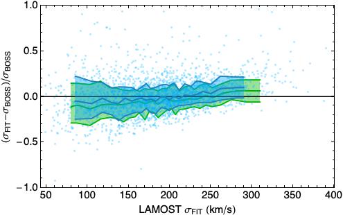
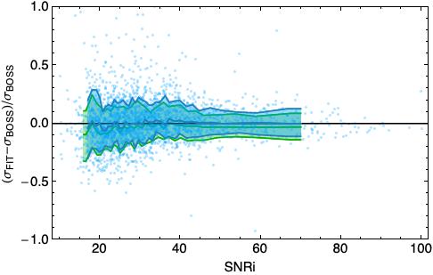
A second difference between SDSS and BOSS is that the latter, differently from SDSS for which we have discussed a lack of relevant systematics, show systematically smaller VDs with respect to BOSS (again with an inverse behaviour only for the lower $n-$index but smaller than the one observed for SDSS – see the upper panel in Fig. 8, left column). This is fully compatible with an aperture effect as the innermost regions sampled by BOSS are more biased toward the maximum of the radial profile of the VD and thus higher than the dispersion measured over a larger aperture, integrating over an area with smaller VD. Again the opposite trend in the lower $n-$index ($<2.5$) is due to some positive VD gradients (see above and Bernardi et al. 2018). In general the LAMOST estimates are about $5-10\%$ smaller than BOSS (e.g. looking at the $\delta\sigma/\sigma$ vs both $n-$index and $R_{e}$ in Fig. 8 bottom), with a mild decreasing trend with the $n-$index and almost no trend with $R_{e}$. In the next section, we discuss in more detail the comparison of the LAMOST estimates and the ones from SDSS and BOSS, after having taken the effect of the aperture correction into account. These aperture corrected values will be also reported in the final velocity dispersion catalog attached to this paper.

To conclude this section on the direct comparison from fiber estimates against SDSS/BOSS, we want to remark that we are not considering other possible sources of scattering: e.g. the effects of site seeing and fiber positioning. While seeing is worth exploring, especially if one wants to use VD measurements for dynamical masses, the fiber positioning is harder to control. One way to check this is to consider whether the larger scattered values are correlated with the difference in SNR between SDSS and LAMOST (as one should expect in case of bad positioning). We did not find any particular trend, hence we concluded that fiber positioning should have a minor impact, at least over large statistical samples.

4.2 Comparison of the estimates after aperture correction

In order to evaluate the possible effect of the fiber sizes on the estimates from the different samples we have re-computed the VDs at the same physical size, the effective radius, also defined as the half-light radius. In particular, we have used the formula by Cappellari et al. (2006) reported here below:

$$\sigma_{\rm R_{e}}=\sigma_{\rm R}(R/R_{e})^{0.066},$$ (2)

although this has been optimized for ETGs and it should be more accurate for $n-$index$>2.5$. We decided to use this simple formula because we have seen in Fig. 8 that the $\delta\sigma/\sigma$ does not significantly depend on the $n-$index, hence one can ignore in the correction the effect of the light profile (although it might matter, see e.g. Bernardi et al. 2018) and consider only the effect of the ratio between the fiber aperture and the radius at which one wants to correct the $\sigma$. Hence despite it represents only an approximation, Eq. 2 has become a standard for this operation (e.g. Tortora et al. 2009; Bezanson et al. 2011; Beifiori et al. 2014; Tortora et al. 2018a; Sonnenfeld 2020).

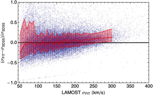
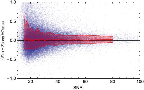
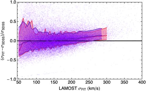
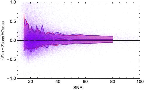
In Fig. 9 we show the $\delta\sigma/\sigma$ before (top panels) and after (bottom panels) of the LAMOST estimated vs. SDSS-DR7 (in LAMOST_SDSS_VD_SERSIC), having applied the aperture correction for both $\sigma_{\rm FIT}$ and $\sigma_{\rm SDSS}$, as a function of the LAMOST VD estimates (left panels) and the sSNR in $i-$band (right panels). In the bottom panels we report the running mean also of the same quantities before the correction for direct comparison. The overall $\delta\sigma/\sigma$ before the correction shows a general agreement among the estimates although some deviation seems to emerge at higher $\sigma_{\rm FIT}$ ($>$200 km/s), while they are fully consistent to each other when plotted against the $SNR_{i}$. The situation does not substantially change after the aperture corrections, which indicates that the fiber diameters ar close enough between LAMOST and SDSS that the aperture correction is statistically indistinguishable from the uncorrected case. Finally the $\delta\sigma/\sigma$ also gives an independent estimate of the statistical errors of the estimates and, consistently with the results from repeated spectra, the scatter in the $\delta\sigma/\sigma$ is a strong function of the $SNR_{i}$ and goes from the 15% relative error at $SNR_{i}>50$ to $\sim$20% at $SNR_{i}=30-40$, while the scatter in the $\delta\sigma/\sigma$ is always $<$25% for $\sigma_{\rm FIT}>100$ km/s, being the scatter quite larger at lower $\sigma_{\rm FIT}$.

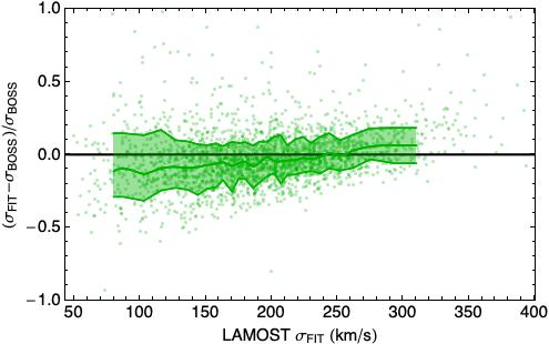
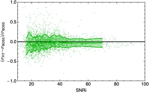
In Fig. 10 we show the same diagnostic as in Fig. 9, but for BOSS galaxies. We can see here some trends quite similar to the ones in the $\delta\sigma/\sigma$ from SDSS, but with a smaller scatter (generally $<15\%$). In particular we notice a small but constant systematic negative offset ($\mathrel{\hbox to0.0pt{\lower 3.5pt\hbox{\hskip 0.5pt$\sim$}\hss}\raise 0.5pt\hbox{$<$}}5\%$) for the VD without the aperture correction, seen especially in the plot against $SNR_{i}$. This is a consequence of the larger differences in the fiber sizes which causes a significant aperture effect. However, as anticipated, the aperture correction renormalizes the estimates and re-aligns the overall trends of the aperture corrected $\delta\sigma/\sigma$ to the behavious found in SDSS. Therefore, using the aperture correction, we could consistently derive VD estimates that look clearly unbiased when plotted against the $SNR_{i}$ (see bottom right panel), but that still shows some (increasing) trend with the $\sigma_{\rm FIT}$, although they are all consistent for $\sigma_{\rm FIT}\mathrel{\hbox to0.0pt{\lower 3.5pt\hbox{\hskip 0.5pt$\sim$}\hss}\raise 0.5pt\hbox{$<$}}250$ km/s, but with a wider consistency with respect to the uncorrected estimates , both in terms of scattering and median values.

5 The Mass–$\sigma$ relation

Galaxies are characterized by striking regularities in their properties, as the correlation between size and mass (e.g. Shen et al. 2003; Hyde & Bernardi 2009a; Roy et al. 2018), or size and surface brightness (e.g. Kormendy 1977; Kormendy et al. 2009; Capaccioli et al. 1992). Then, there exist specific relationships for early-type galaxies, as the Fundamental Plane (e.g., Djorgovski & Davis 1987; Dressler et al. 1987; Hyde & Bernardi 2009b) and the Faber-Jackson relation (Faber & Jackson 1976) or those for late-type systems, as the Tully-Fisher relation (e.g. Tully & Fisher 1977; Lelli et al. 2016). The study of these correlations, their evolution with redshift and the comparison with theoretical predictions provide crucial information about the galaxy formation and evolution processes, as demonstrated by the analysis of size and velocity dispersion evolution in massive early-type galaxies (e.g. Fan et al. 2008; Cenarro & Trujillo 2009; Hopkins et al. 2009; Tortora et al. 2014c, 2018a; Roy et al. 2018).

Figure 11: Top: the absolute luminosity$-$size relation of the LAMOST galaxies with available structural parameters. Galaxies are classified as ETGs (red), and LTGs (blue) according to their $n-$index. Isodensity contours in the parameter space are overplotted with the same color code. Bottom: the mean $\langle\mu_{e,r}\rangle$$-$$R_{e}$ relation of the same galaxy samples (ETGs, red points, and LTGs, blue points). Isodensity contours in the parameter space are overplotted with the same color code. The black solid line is the best fit to the $\langle\mu_{e,r}\rangle$$-$$R_{e}$ ($r-$band) relation of a local SDSS sample of ETGs from Lackner & Gunn (2012).

Figure 12: Left: Mass distribution of galaxies classified as ETGs (red), and LTGs (blue). They both show a pseudo-normal distribution. Short vertical lines show the 75% relative completeness of the LAMOST sample (see right panel). Right: relative completeness of the LAMOST galaxies with respect to the total sample for the ETG sample (red squares) and the LTG sample (blue squares), as defined according to their $n-$index, see text. The horizontal line shows the 75% relative completeness corresponding to a mass limit where 50% of the galaxies are lost with respect to the peak. Overplotted the best-fit error function, with the $\pm 1\sigma$ confidence curves from the best-fit parameters (see discussion in the text)

Therefore, as a demonstration of the scientific validity of the dataset produces from LAMOST-DR7, we derive in this section the Mass-$\sigma$ relation for the LAMOST-DR7 galaxies and compare the results with independent analyses (e.g. Nigoche-Netro et al. 2011, Tortora et al. 2014c). The Mass–$\sigma$ relation is a fundamental scaling relation for galaxies and it has been demonstrated to vary as a function of the galaxy properties (e.g. Graves et al. 2009) and as a function of redshift (e.g. Nigoche-Netro et al. 2011). We stress here that the following analysis, based on our newly derived VDs of LAMOST galaxies, is aimed at deriving the general trend of the relation to validate the dataset rather than fully tackle the physics behind the relation, including the variation with redshift. This will be the content of future analyses.

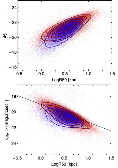
To derive the Mass–$\sigma$ relation for the LAMOST sample We have combined both the LAMOST_SDSS_VD_SERSIC and LAMOST_BOSS_VD_SERSIC catalogs for which we have 1) the aperture corrected VD estimates in §4.2 and 2) updated stellar masses, using star forming models according to Maraston et al. (2009), are provided by the SDSS Sky Server (stellarMassStarformingPort). The match of the VD catalog with the stellar mass catalog has given 53 308 entries. We used these stellar mass models because a large part of our sample is made of LTGs as we could classify according to the $n-$index. Indeed, ETGs are roughly separated from LTGs, assuming $n>2.5$ for the former and $n\leq 2.5$ for the latter (Roy et al. 2018). Using this criterion we have found 37 494 ETGs and 15 814 LTGs. To illustrate the photometric properties of these galaxy samples, in Fig. 11 we show two classical scaling relations: the magnitude–size relation and the $\langle\mu_{e,r}\rangle$$-$$R_{e}$ relation (see also Graham 2019 for a compelling review). As the LAMOST galaxies cover a fair range of redshift (see Fig. 2), absolute magnitudes in $r-$band have been obtained by applying a $k-$correction to the $r-$band apparent magnitudes. We have grouped the galaxies in 5 redshift bins (from 0.1 to 0.5 in steps of $\Delta z=$0.1) and used the mean reshift of the bin and the individual galaxy $g-r$ colours to obtain the $k_{r}(z,g-r)$. Then these values have been used to derive the absolute magnitude in $r-$band defined as $M_{r}=m_{r}-5\,{\rm Log}\,D_{L}/10pc-k_{r}$, where $D_{L}$ is the luminosity distance derived by the LAMOST redshift estimates. We have also applied the same $k_{r}-$correction to the mean surface brightness, defined as $\langle\mu_{e,r}\rangle=(m_{r}-k_{r})+2.5\,{\rm Log}\,2\pi+5\,{\rm Log}\,R_{e}$.

Albeit qualitative, the plots show regular trends of the ETGs which lie on a sequence that is different than the one of LTGs in both diagrams (see e.g. Gadotti 2009). Galaxies selected as LTGs are generally fainter and possess lower mean surface brightness in their centers (Pierini et al. 2002, see also Luo et al. 2020). The trends of LAMOST galaxies, though, incorporate some variation of the relations due to the variation with redshift of galaxy properties ($M_{r}$, $\langle\mu_{e,r}\rangle$, $R_{e}$). A full discussion of the dependence on redshift of these relations and its physical interpretation is beyond the purpose of this analysis, where we want to focus on the Mass–size relation, and it will be addressed in a forthcoming paper. However, in the bottom panel of the figure, we overplot the best fit to the $\langle\mu_{e}\rangle$$-$$R_{e}$ ($r-$band) relation of a local SDSS sample of ETGs from Lackner & Gunn (2012). This shows an overall agreement with the LAMOST galaxies’ relation, although their selection of ETGs is slightly more stringent than ours ($n-index=4$).

Figure 13: Mass–$\sigma$ relation from LAMOST galaxies, separated in ETGs (upper panels, red dots) and LTGs (lower panels blue dots). Velocity dispersion values are aperture corrected to match the value at the effective radius as in §2.3. Left panels: points with error bars are median and median deviation respectively of the binned data points, along the X-axis and the Y-axis. Solid lines (red on the top and blue on the bottom) are the weighted linear fit to the median values (see text for details) with the best fit values given in Table 2. The lighter colored data points (orange in the top panel and light blue in the bottom panel) show the data above the completeness lines (see text for details and right panels). Right panels: density contours in the Mass–$\sigma$ space of the ETGs (top) and LTG (bottom). In both panels we report the best fit obtained from the median values, as in the left panel. For ETGs we also report literature relations from Nigoche-Netro et al. (2011) (black line) and a collection of best fit relations from Tortora et al. (2014c) (gray lines, see text for the full description).

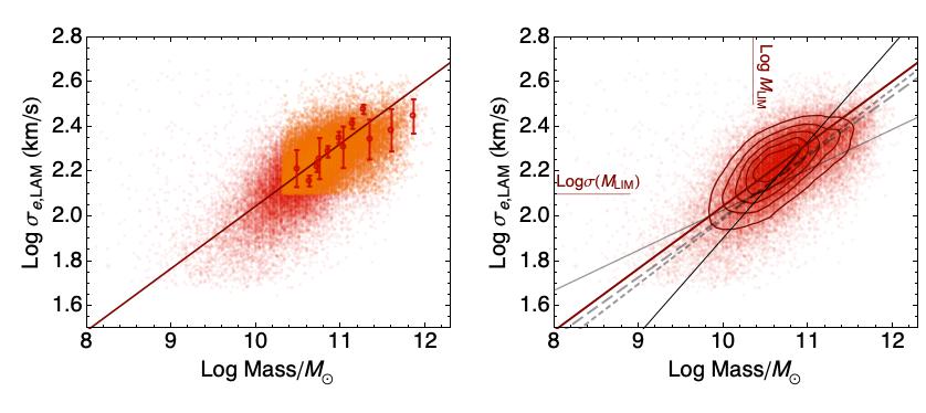
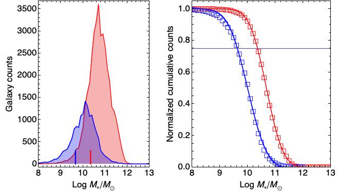
Moving to the Mass–$\sigma$ relation, in order to derive an unbiased trend we need to estimate a limiting mass below which we start loosing a significant number of galaxies with respect to the peak value. Following the procedure adopted in §2.3, we have used Eq. 1 to evaluate the mass at which the number of galaxies decreases at about 50% from the peak. This is obtained by finding the mass at which the cumulative mass function shown in Fig. 12 equals 0.75. We have fitted the distributions of the ETGs and LTGs with the function 1-comp${x}$ as in Eq. 1, where now the variable is the decreasing mass, and obtained $\log M_{*}/M_{\odot}=10.35\pm 0.01$ and $\log M_{*}/M_{\odot}=9.63\pm 0.01$ for ETG sand LTGs respectively.

$\log\sigma_{e}=a+b\log M_{*}/M_{\odot}$
Type	$a$	$b$	significance
ETGs	$-0.7\pm 0.6$	$0.28\pm 0.06$	$1\sigma$
LTGs	$-1.8\pm 0.7$	$0.38\pm 0.07$	$1\sigma$

Table 2: Weighted linear fit to the Mass-$\sigma$ relation, according to the Eq. 3

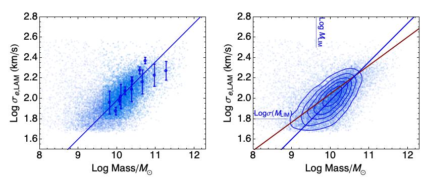
In Fig. 13 we show the Mass, $\log M_{\rm*}/M_{\odot}$, vs. the LAMOST velocity dispersion values corrected to the effective radius aperture, $\log\sigma_{\rm e,~{}LAM}$, for the two galaxy types, ETGs (in red) and the LTGs (in blue). We also show the best fit linear relation to the galaxies above the limiting mass, $M_{\rm lim}$, and the average VD value ($\log\sigma(M_{\rm lim})$), i.e. the mean velocity dispersion that we have estimated for 400 galaxies in a bin around $M_{\rm lim}$. These are both indicated in the graph in order to evaluate the range adopted for the linear fit for ETGs and LTGs.

In order to mitigate biases in the linear fit due to the incompleteness both in mass and sigma, we have performed a linear fit over the median values we have derived binning the data along the X-axis and Y-axis, as indicated by the two groups of data with error bars (MAD/0.6745) in Fig. 13 (left panels for ETGs and LTGs, on top and bottom respectively). The linear formula adopted is

$$\log\sigma_{e}=a+b\log{M_{*}/M_{\odot}}$$ (3)

and the best fit parameters are reported in Table 2, where we have used the inverse of the errors on the median points as weights. From the values of the slope ($b$) we see that the two samples are barely consistent to each other within $1\sigma$. We notice though that our fitting procedure is rather conservative, as it incorporates in its scatter the systematic of the trend in both variables.

We can compare these results with previous findings from local samples. In Fig. 13 we show the relation found for different samples: 1) a volume limited sample of ETGs from the NYU-VAGC from Nigoche-Netro et al. (2011, N+11, solid black line), for which masses have been estimated from galaxy colours using the relation from Bell et al. (2003); 2) a collection of Mass-$\sigma$ relations from Tortora et al. (2014c, T+14, see their Table 1), which has analysed data from different local samples from Tortora et al. (2009, T+09, long dashed gray), Cappellari et al. (2013a, b, Atlas3D, short dashed gray) and Tortora et al. (2012a, SPIDER sample, solid gray). We see that our ETG estimates are in a substantial agreement with the T+09 and ATLAS3D samples, in particular they show a very similar slope ($0.27\pm 0.01$, $0.29\pm 0.02$ respectively, from Table 1 of T+14, vs. $0.28\pm 0.06$ from out Table 2), while a small offset in mass is also visible due to difference in mass inferences. A more significant tilt of the slopes of both the N+11 and SPIDER samples is evident. This might have some different origins. For N+11, they do not discuss the use of an aperture correction, hence part of the tilt might come from the aperture correction. For SPIDER, their analysis is more focused on the massive sample, hence their slope is more sensitive to the region of the relationship that shows a knee, at $\log M_{*}/M_{\odot}~{}\hbox to0.0pt{$>$\hss}{\lower 4.30554pt\hbox{$\sim$}}10.6$.

For LTGs there are little reference in literature to compare our results to: for instance, we have found that our best fit parameters in Table 2 lie in between best fit Mass–$\sigma$ relations by Mogotsi & Romeo (2019, e.g. their Table 3) from 34 nearby spirals from the Calar Alto Legacy Integral Field Area (CALIFA) survey.

Curvatures and bendings in galaxy scaling relations are emerging at some characteristic mass scales. Virial mass (e.g. Moster et al. 2010), size (Hyde & Bernardi, 2009a), central DM fraction and total mass density slope (Cappellari et al., 2013b; Tortora et al., 2019), optical colour, metallicity and stellar M/L gradient (Spolaor et al., 2010; Tortora et al., 2010a, 2011) present bendings or upturn/downturn at $\mbox{$M_{\star}$}\sim 3\times 10^{10}\,\rm M_{\rm\odot}$ (Chabrier IMF). Such correlations are shaped by different kinds of physical processes which can be regulated by this characteristic mass (Tortora et al. 2019).

Our Mass-$\sigma$ relation also shows a bending signature, which is more evident in Fig. 14, where we combine all results from this work and previous literature relations. Here we see that the two samples of galaxies, ETGs and LTGs, albeit separated simplistically through their $n-$index, show two main features: 1) they seem to lie on a similar relation at masses lower than $\log M_{*}/M_{\odot}~{}\hbox to0.0pt{$>$\hss}{\lower 4.30554pt\hbox{$\sim$}}10.6$ (Kroupa IMF), while ETGs sit on a shallower relation at masses higher than $\log M_{*}/M_{\odot}~{}\hbox to0.0pt{$>$\hss}{\lower 4.30554pt\hbox{$\sim$}}10.6$, which determines the shallower overall slope found in Table 2 and drawn by the best–fit curve. If one would select a more massive sample, an even shallower slope might be found (see e.g. Tortora et al. 2012a). This will be investigated in mode details in forthcoming analyses.

Indeed, a full discussion of the Mass-$\sigma$ relation is beyond the purpose of this paper, which is partially based on publicly available data (e.g. masses) which we cannot fully control.

Figure 14: Mass–$\sigma$ relation from LAMOST galaxies from Fig. 13: ETGs (red dots) and LTGs (blue dots). Galaxies with different $n-$index show a different slope as demonstrated by the red and blue solid lines. The slope of the ETG sample is nicely consistent with local samples from Tortora et al. (2014c) (short and long dashed gray lines) but slightly tilted with respect to the SPIDER/SDSS sample from Tortora et al. (2012a) (solid gray line) and Nigoche-Netro et al. (2011) (solid black line).

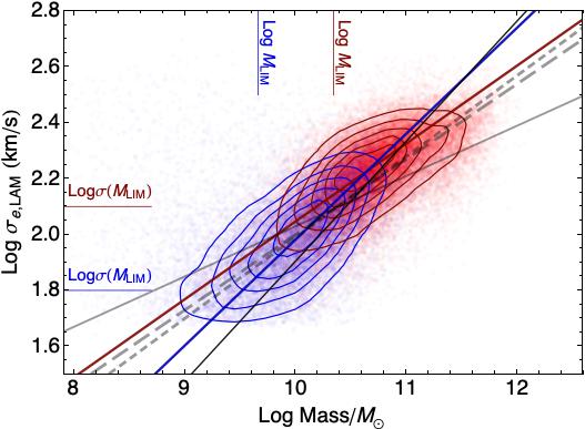
Here we just remark that, despite all inhomogeneities with other datasets, the fact that the best fit relations are very similar and statistically consistent (in the range of mass above the limiting mass of the LAMOST sample) with external datasets demonstrates that LAMOST VD estimates are robust for further science exploitation.

6 Conclusions

We have produced the first catalog of velocity dispersion measurements for galaxies belonging to the LEGAS sample observed with LAMOST. The catalog is based on the spectra delivered with the LAMOST-DR7. This includes 193 361 spectra classified as galaxy-type which are distributed over $\sim 11\,500$ deg² of the sky and overlap with other imaging (SDSS, HSC) and spectroscopic (BOSS) surveys. After a quality selection, largely based on a conservative cut in SNR in $g-$ and $i-$ band. We have adopted a wrap-up procedure to perform the spectral fitting using pPXF, and derive velocity dispersion measurements. After applying further quality criteria, like signal-to-the-residual ratio (SRR)>5, the $\chi^{2}_{\rm FIT}$ < 1.1 and a velocity dispersion range of 50 km/s $\leq\sigma_{\rm meas}\leq$ 450 km/s, we have collected central velocity dispersion measurements of $\sim 86\,000$ galaxies, which we make publicly available. About 50 500 of these galaxies have a match with SDSS and $\sim$2600 with BOSS, and have structural parameters (e.g. Sérsic Index, effective radius, Petrosian magnitudes) and stellar masses available from literature (e.g. NYU-VAGC, SDSS). For the other galaxies similar quantities need to be derived from suitable ancillary datasets.

We have estimated statistical errors as a function of the SNR using both duplicated spectra of individual galaxies from LAMOST (Fig. 6) and compared the relative scatter of LAMOST estimates against a common sample of SDSS and BOSS galaxies (Fig. 9 and Fig. 10) and they all consistently show that internal statistical errors are always within 20% at SNR$>20$ and down to $\mathrel{\hbox to0.0pt{\lower 3.5pt\hbox{\hskip 0.5pt$\sim$}\hss}\raise 0.5pt\hbox{$<$}}$15% for SNR$>50$. In the same figures, we can also see that after having corrected the VD estimate for fiber apertures and computed the velocity dispersion at the effective radius, we have found almost no systematics between the LAMOST estimates and SDSS and BOSS, as a function of both the LAMOST velocity dispersion values and the SNR.

Finally as a scientific validation of the new VD catalog, in combination with other ancillary data, we have derived the Mass$-\sigma$ relation of the LAMOST dataset after having separated early-type galaxies (ETGs) from late-type galaxies (LTGs) solely on the basis of their Sérsic-index, and compared with other literature studies. We have found a substantial agreement of the slope of the relation of the ETGs with other local samples (see Fig. 14), largely based on SDSS data, from Nigoche-Netro et al. (2011) and Tortora et al. (2014c), while LTGs show a steeper slope (also in Fig. 14, but see also Tab 2), although significant only at about 2$\sigma$ level.

We plan to develop the machinery presented here with a more sophisticated analysis, implementing 1) a resampling the LAMOST spectra and 2) a bootstrap of pPXF set-up in order to associate more realistic errors to the VD estimates and to minimize the source of systematics.

With this first analysis we have demonstrated that LAMOST spectra are suitable for galaxy kinematics. This represents a value added product for the LAMOST project but has also a legacy value because it has a large overlap with SDSS/BOSS in the NGC, and provides first VD estimates for galaxies in a large area in the SGC, which will be soon targeted by optical/NIR space facilities like EUCLID and the Chinese Space Station Telescope.

Appendix A Preliminary tests on pPXF bootstrapping and template mismatch

In the §3.1.2, we have illustrated the pPXF set-up adopted for this first VD catalog from LAMOST spectra and anticipated what are the pipeline improvements that we plan to implement for future analyses. In particular we plan to obtain average estimates and realistic statistical errors by bootstrapping over different pPXF set-up and resampling the LAMOST spectra using the spectral noise. As a first quick test on the outcome of this analysis, we have experimented a preliminary procedure over a limited sample.

The procedure randomly creates 256 realizations of each observed spectrum by adding Gaussian noise to each pixel and by randomly shifting (to bluer or redder wavelengths) the selected restframe wavelength window of the spectrum by a maximum of 10 pixels. It also varies a series of fitting parameters like the LOSVD moments, the degree of additive polynomials, and the initial guesses of radial velocity and velocity dispersion, (see D’Ago et al., in preparation).

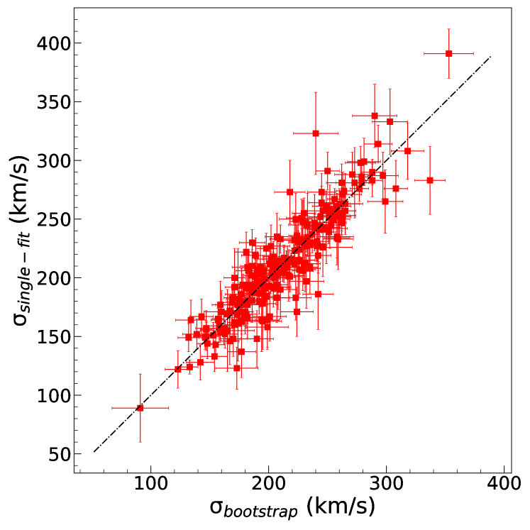
In Fig. 15, we demonstrate the results for $\sim 200$ galaxies, where the single pPXF measurements are plotted against the bootstrap average value (errorbars are the standard deviation over the 256 realizations). As it is seen the estimates nicely sit on the one-to-one correlation (solid line) with average relative scatter of $\sim$0.13, e.g. consistent with the one found in the repeated spectra experiment in Figs. 6 and 7 (see §3.2.2). The reason of such a very good accuracy of the single measurement, despite some simplistic assumptions, e.g. about initial conditions and the number of templates (i.e. the use of 40 MILES SSP models from Vazdekis et al. 2010, see also below) resides on the quite high SNR and good resolution of the LAMOST spectra. The full bootstrap procedure, though, will return more realistic errors associated to the VD values. Also, it will be necessary to assess internal statistical errors and systematics in case we will adopt looser constraint on the SNR spectra quality overall, to increase the completeness of the VD catalog in future releases.

Figure 15: Preliminary bootstrap test over a sample of $\sim 200$ LAMOST galaxies. Comparison between the single run pPXF VD estimates and the ones obtained over the bootstrap procedure where 256 are averaged after LAMOST spectra are resampled, the pPXF parameters are randomly changed and the stellar templates are also picked across the MILES catalog. See text for more details. The solid line represents the one-to-one relation.

Finally, a note about the template choice. Stellar template mismatch is one limiting factor for velocity dispersion accuracy. In the current analyses we have used a selection of 40 MILES SSP models, covering a wide range of metallicities (0.02$\leq Z/Z_{\odot}\leq$1.58) and ages (between 1 Gyr and 13 Gyr). In principle we could have used single star templates (e.g. among the 268 empirical stars from MILES library, uniformly sampling effective temperature, metallicity and surface gravity of the full catalogue of templates), but at the cost of a much longer computing time. However, we have checked in previous analyses (e.g. Scognamiglio et al. 2020) that this does not affect considerably the VD results. However, we will address this effect more in details in future analyses.

Appendix B Redshift consistency

Source redshifts are the basic entries of the LAMOST data releases, for all spectra and classes of objects. This paper aims at providing the first catalog of velocity dispersion estimates as an additional kinematical parameter to the standard LAMOST catalog entries. Of course, when performing the template fitting to the spectra, the assumed velocity distribution (which we have set to be Gaussian in this first VD release) incorporates the mean redshift as a fitting parameter. Hence, we provide, as an output of the VD catalog, the difference between the LAMOST pipeline released redshift and the estimated pPXF one, $\Delta z$ (see §3.2.3) for all galaxies with SNR${}_{i}>10$ or SNR${}_{g}>10$. For all other galaxies (and other source types) with SNR<10, the redshifts are still retrievable by the LAMOST-DR7 general release.

Figure 16: Redshift consistency between the pPXF estimates and the ones of the original LAMOST catalog ($\Delta z$), and the redshifts from SDSS and BOSS systems matching with the LAMOST VD catalog ($\Delta z_{\rm SDSS}$). Top row. The ($\Delta z$) distribution (left) and the $\Delta z_{\rm SDSS}$ (right) showing an offset with respect to zero. Bottom row. The relative scatter of the LAMOST VD estimates (as defined in §4) versus $\Delta z$ (left) and $\Delta z_{\rm SDSS}$ (right) showing no evident correlations in both cases.

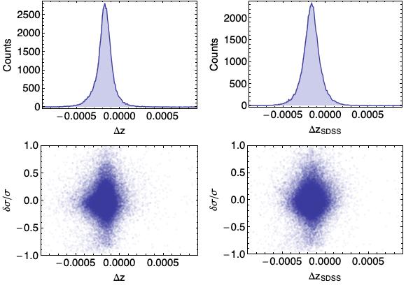
For sake of completeness, in this appendix, we briefly quantify the $\Delta z$, introduced in §3.2.3, although any detailed discussion of discrepancies among pipelines is beyond the purpose of this paper, unless they affect the VD estimates. The distribution of the $\Delta z$ is reported in Fig. 16 (top-left). Here we see that $\Delta z$ are oddly distributed with respect to $\Delta z=0$, with a median value of the $\langle\Delta z\rangle=-0.00018\pm 0.00009$, i.e. $\sim 2\sigma$ larger than zero, meaning that there is a significant offset. The origin of this systematic difference remains unclarified, and it is also present in the $\Delta z_{\rm SDSS}$ with SDSS/BOSS (defined as $\Delta z_{\rm SDSS}=z_{\rm SDSS}-Z_{\rm ppxf}$ and also shown in Fig. 16), which is $-0.00017\pm 0.00010$. This means that this systematic effect has been introduced by the pPXF procedure. However, this is not worrisome as long as we can demonstrate that it does not introduce any systematic on the VD estimates.

In the same Fig. 16 we plot the VD scatter of the LAMOST/pPXF estimates vs. SDSS/BOSS, as a function of the $\Delta z_{\rm LAM}$ and $\Delta z_{\rm SDSS}$. We do not measure any correlation in both cases, which means that the overall VD estimates reported in the catalog are unaffected by this offset, which we plan to solve in the next releases.

References

- Ahn et al. (2012) Ahn C. P., et al., 2012, ApJS, 203, 21
- Ai et al. (2016) Ai Y. L., et al., 2016, AJ, 151, 24
- Aihara et al. (2018) Aihara H., et al., 2018, PASJ, 70, S4
- Alpaslan et al. (2015) Alpaslan M., et al., 2015, MNRAS, 451, 3249
- Auger et al. (2010a) Auger M. W., Treu T., Gavazzi R., Bolton A. S., Koopmans L. V. E., Marshall P. J., 2010a, ApJ, 721, L163
- Auger et al. (2010b) Auger M. W., Treu T., Bolton A. S., Gavazzi R., Koopmans L. V. E., Marshall P. J., Moustakas L. A., Burles S., 2010b, ApJ, 724, 511
- Bautista et al. (2018) Bautista J. E., et al., 2018, ApJ, 863, 110
- Beifiori et al. (2014) Beifiori A., et al., 2014, ApJ, 789, 92
- Bell et al. (2003) Bell E. F., McIntosh D. H., Katz N., Weinberg M. D., 2003, ApJS, 149, 289
- Bernardi et al. (2018) Bernardi M., Sheth R. K., Dominguez-Sanchez H., Fischer J. L., Chae K. H., Huertas-Company M., Shankar F., 2018, MNRAS, 477, 2560
- Bezanson et al. (2011) Bezanson R., et al., 2011, ApJ, 737, L31
- Blanton et al. (2005) Blanton M. R., et al., 2005, AJ, 129, 2562
- Capaccioli et al. (1992) Capaccioli M., Caon N., D’Onofrio M., 1992, MNRAS, 259, 323
- Cappellari (2017) Cappellari M., 2017, MNRAS, 466, 798
- Cappellari et al. (2006) Cappellari M., et al., 2006, MNRAS, 366, 1126
- Cappellari et al. (2013a) Cappellari M., et al., 2013a, MNRAS, 432, 1709
- Cappellari et al. (2013b) Cappellari M., et al., 2013b, MNRAS, 432, 1862
- Cardone & Tortora (2010) Cardone V. F., Tortora C., 2010, MNRAS, 409, 1570
- Cardone et al. (2009) Cardone V. F., Tortora C., Molinaro R., Salzano V., 2009, A&A, 504, 769
- Cavuoti et al. (2015) Cavuoti S., et al., 2015, MNRAS, 452, 3100
- Cavuoti et al. (2017) Cavuoti S., et al., 2017, MNRAS, 466, 2039
- Cenarro & Trujillo (2009) Cenarro A. J., Trujillo I., 2009, ApJ, 696, L43
- Chabrier (2001) Chabrier G., 2001, ApJ, 554, 1274
- Chambers et al. (2016) Chambers K. C., et al., 2016, arXiv e-prints, p. arXiv:1612.05560
- Colless et al. (2001) Colless M., et al., 2001, MNRAS, 328, 1039
- Costantin et al. (2019) Costantin L., et al., 2019, A&A, 632, A9
- Cui et al. (2012) Cui X.-Q., et al., 2012, Research in Astronomy and Astrophysics, 12, 1197
- Dawson et al. (2013) Dawson K. S., et al., 2013, AJ, 145, 10
- Deng et al. (2012) Deng L.-C., et al., 2012, Research in Astronomy and Astrophysics, 12, 735
- Djorgovski & Davis (1987) Djorgovski S., Davis M., 1987, ApJ, 313, 59
- Dressler et al. (1987) Dressler A., Lynden-Bell D., Burstein D., Davies R. L., Faber S. M., Terlevich R., Wegner G., 1987, ApJ, 313, 42
- Driver et al. (2016) Driver S. P., Davies L. J., Meyer M., Power C., Robotham A. S. G., Baldry I. K., Liske J., Norberg P., 2016, in Napolitano N. R., Longo G., Marconi M., Paolillo M., Iodice E., eds, Vol. 42, The Universe of Digital Sky Surveys. p. 205 (arXiv:1507.00676), doi:10.1007/978-3-319-19330-4_32
- Du et al. (2019) Du B., et al., 2019, ApJS, 240, 10
- Dutton & Treu (2014) Dutton A. A., Treu T., 2014, MNRAS, 438, 3594
- Faber & Jackson (1976) Faber S. M., Jackson R. E., 1976, ApJ, 204, 668
- Fan et al. (2008) Fan L., Lapi A., De Zotti G., Danese L., 2008, ApJ, 689, L101
- Feng et al. (2019) Feng S., et al., 2019, ApJ, 880, 114
- Gadotti (2009) Gadotti D. A., 2009, MNRAS, 393, 1531
- Graham (2019) Graham A. W., 2019, Publ. Astron. Soc. Australia, 36, e035
- Graves et al. (2009) Graves G. J., Faber S. M., Schiavon R. P., 2009, ApJ, 698, 1590
- Guzzo & Vipers Team (2017) Guzzo L., Vipers Team 2017, The Messenger, 168, 40
- Hamabe & Kormendy (1987) Hamabe M., Kormendy J., 1987, in de Zeeuw P. T., ed., IAU Symposium Vol. 127, Structure and Dynamics of Elliptical Galaxies. p. 379
- Hildebrandt et al. (2017) Hildebrandt H., et al., 2017, MNRAS, 465, 1454
- Hopkins et al. (2009) Hopkins P. F., Hernquist L., Cox T. J., Keres D., Wuyts S., 2009, ApJ, 691, 1424
- Hopkins et al. (2013) Hopkins A. M., et al., 2013, MNRAS, 430, 2047
- Huang et al. (2014) Huang Y., et al., 2014, MNRAS, 439, 2927
- Huertas-Company et al. (2013) Huertas-Company M., et al., 2013, MNRAS, 428, 1715
- Hyde & Bernardi (2009a) Hyde J. B., Bernardi M., 2009a, MNRAS, 394, 1978
- Hyde & Bernardi (2009b) Hyde J. B., Bernardi M., 2009b, MNRAS, 396, 1171
- Jones et al. (2009) Jones D. H., et al., 2009, MNRAS, 399, 683
- Kormendy (1977) Kormendy J., 1977, ApJ, 218, 333
- Kormendy et al. (2009) Kormendy J., Fisher D. B., Cornell M. E., Bender R., 2009, ApJS, 182, 216
- Krajnović et al. (2011) Krajnović D., et al., 2011, MNRAS, 414, 2923
- Kroupa (2001) Kroupa P., 2001, MNRAS, 322, 231
- Kuijken et al. (2019) Kuijken K., et al., 2019, A&A, 625, A2
- La Barbera et al. (2010) La Barbera F., de Carvalho R. R., de La Rosa I. G., Lopes P. A. A., 2010, MNRAS, 408, 1335
- Lackner & Gunn (2012) Lackner C. N., Gunn J. E., 2012, MNRAS, 421, 2277
- Lam et al. (2015) Lam M. I., et al., 2015, Research in Astronomy and Astrophysics, 15, 1424
- Lelli et al. (2016) Lelli F., McGaugh S. S., Schombert J. M., 2016, ApJ, 816, L14
- Liske et al. (2015) Liske J., et al., 2015, MNRAS, 452, 2087
- Luo et al. (2012) Luo A. L., et al., 2012, Research in Astronomy and Astrophysics, 12, 1243
- Luo et al. (2015) Luo A. L., et al., 2015, Research in Astronomy and Astrophysics, 15, 1095
- Luo et al. (2020) Luo Y., et al., 2020, MNRAS, 493, 1686
- Maraston et al. (2009) Maraston C., Strömbäck G., Thomas D., Wake D. A., Nichol R. C., 2009, MNRAS, 394, L107
- Miyazaki et al. (2012) Miyazaki S., et al., 2012, Hyper Suprime-Cam. p. 84460Z, doi:10.1117/12.926844
- Mogotsi & Romeo (2019) Mogotsi K. M. and Romeo A. B.,2019, MNRAS, 489, 3797
- Moster et al. (2010) Moster B. P., Somerville R. S., Maulbetsch C., van den Bosch F. C., Macciò A. V., Naab T., Oser L., 2010, ApJ, 710, 903
- Napolitano et al. (2010) Napolitano N. R., Romanowsky A. J., Tortora C., 2010, MNRAS, 405, 2351
- Newman et al. (2013) Newman J. A., et al., 2013, ApJS, 208, 5
- Nigoche-Netro et al. (2011) Nigoche-Netro A., Aguerri J. A. L., Lagos P., Ruelas-Mayorga A., Sánchez L. J., Muñoz-Tuñón C., Machado A., 2011, A&A, 534, A61
- Pierini et al. (2002) Pierini D., Gavazzi G., Franzetti P., Scodeggio M., Boselli A., 2002, MNRAS, 332, 422
- Roy et al. (2018) Roy N., et al., 2018, MNRAS, 480, 1057
- Rykoff et al. (2015) Rykoff E. S., Rozo E., Keisler R., 2015, arXiv e-prints, p. arXiv:1509.00870
- Salpeter (1955) Salpeter E. E., 1955, ApJ, 121, 161
- Salviander & Shields (2013) Salviander S., Shields G. A., 2013, ApJ, 764, 80
- Saulder et al. (2015) Saulder C., van den Bosch R. C. E., Mieske S., 2015, A&A, 578, A134
- Scognamiglio et al. (2020) Scognamiglio D., et al., 2020, arXiv e-prints, p. arXiv:2002.12922
- Sersic (1968) Sersic J. L., 1968, Atlas de Galaxias Australes
- Shen et al. (2003) Shen S., Mo H. J., White S. D. M., Blanton M. R., Kauffmann G., Voges W., Brinkmann J., Csabai I., 2003, MNRAS, 343, 978
- Shen et al. (2016) Shen S.-Y., et al., 2016, Research in Astronomy and Astrophysics, 16, 43
- Shi et al. (2014a) Shi Z.-X., et al., 2014a, Research in Astronomy and Astrophysics, 14, 1234
- Shi et al. (2014b) Shi Z. X., Comte G., Luo A. L., Zhao Y. H., Zhao J. K., Oswalt T. D., Wu F. C., 2014b, A&A, 564, A89
- Sonnenfeld (2020) Sonnenfeld A., 2020, arXiv e-prints, p. arXiv:2002.01940
- Sonnenfeld et al. (2015) Sonnenfeld A., Treu T., Marshall P. J., Suyu S. H., Gavazzi R., Auger M. W., Nipoti C., 2015, ApJ, 800, 94
- Spiniello et al. (2015) Spiniello C., Barnabè M., Koopmans L. V. E., Trager S. C., 2015, MNRAS, 452, L21
- Spolaor et al. (2010) Spolaor M., Kobayashi C., Forbes D. A., Couch W. J., Hau G. K. T., 2010, MNRAS, 408, 272
- Stoughton et al. (2002) Stoughton C., et al., 2002, AJ, 123, 485
- The Dark Energy Survey Collaboration (2005) The Dark Energy Survey Collaboration 2005, arXiv e-prints, pp astro–ph/0510346
- Thomas et al. (2009) Thomas J., Saglia R. P., Bender R., Thomas D., Gebhardt K., Magorrian J., Corsini E. M., Wegner G., 2009, ApJ, 691, 770
- Thomas et al. (2011) Thomas J., et al., 2011, MNRAS, 415, 545
- Thomas et al. (2013) Thomas D., et al., 2013, MNRAS, 431, 1383
- Tortora et al. (2009) Tortora C., Napolitano N. R., Romanowsky A. J., Capaccioli M., Covone G., 2009, MNRAS, 396, 1132
- Tortora et al. (2010a) Tortora C., Napolitano N. R., Cardone V. F., Capaccioli M., Jetzer P., Molinaro R., 2010a, MNRAS, 407, 144
- Tortora et al. (2010b) Tortora C., Napolitano N. R., Romanowsky A. J., Jetzer P., 2010b, ApJ, 721, L1
- Tortora et al. (2011) Tortora C., Napolitano N. R., Romanowsky A. J., Jetzer P., Cardone V. F., Capaccioli M., 2011, MNRAS, 418, 1557
- Tortora et al. (2012a) Tortora C., La Barbera F., Napolitano N. R., de Carvalho R. R., Romanowsky A. J., 2012a, MNRAS, 425, 577
- Tortora et al. (2013) Tortora C., Romanowsky A. J., Napolitano N. R., 2013, ApJ, 765, 8
- Tortora et al. (2014a) Tortora C., Romanowsky A. J., Cardone V. F., Napolitano N. R., Jetzer P., 2014a, MNRAS, 438, L46
- Tortora et al. (2014b) Tortora C., La Barbera F., Napolitano N. R., Romanowsky A. J., Ferreras I., de Carvalho R. R., 2014b, MNRAS, 445, 115
- Tortora et al. (2014c) Tortora C., Napolitano N. R., Saglia R. P., Romanowsky A. J., Covone G., Capaccioli M., 2014c, MNRAS, 445, 162
- Tortora et al. (2018a) Tortora C., Napolitano N. R., Roy N., Radovich M., Getman F., Koopmans L. V. E., Verdoes Kleijn G. A., Kuijken K. H., 2018a, MNRAS, 473, 969
- Tortora et al. (2018b) Tortora C., Koopmans L. V. E., Napolitano N. R., Valentijn E. A., 2018b, MNRAS, 473, 2324
- Tortora et al. (2018c) Tortora C., et al., 2018c, MNRAS, 481, 4728
- Tortora et al. (2019) Tortora C., Posti L., Koopmans L. V. E., Napolitano N. R., 2019, arXiv e-prints,
- Tully & Fisher (1977) Tully R. B., Fisher J. R., 1977, A&A, 54, 661
- Vazdekis et al. (2010) Vazdekis A., Sánchez-Blázquez P., Falcón-Barroso J., Cenarro A. J., Beasley M. A., Cardiel N., Gorgas J., Peletier R. F., 2010, MNRAS, 404, 1639
- Wang et al. (1996) Wang S.-G., Su D.-Q., Chu Y.-Q., Cui X., Wang Y.-N., 1996, Appl. Opt., 35, 5155
- Wang et al. (2018) Wang L.-L., et al., 2018, MNRAS, 474, 1873
- Wang et al. (2019) Wang M. X., et al., 2019, MNRAS, 482, 1889
- Xiang et al. (2015) Xiang M. S., et al., 2015, MNRAS, 448, 822
- Yang et al. (2015) Yang H.-F., et al., 2015, Research in Astronomy and Astrophysics, 15, 1414
- Yang et al. (2018) Yang M., et al., 2018, ApJS, 234, 5
- Zhao et al. (2012) Zhao G., Zhao Y.-H., Chu Y.-Q., Jing Y.-P., Deng L.-C., 2012, Research in Astronomy and Astrophysics, 12, 723
- Zhao et al. (2019) Zhao P.-S., et al., 2019, Research in Astronomy and Astrophysics, 19, 113
- Zheng & Shen (2020) Zheng Y.-L., Shen S.-Y., 2020, ApJS, 246, 12