\declaretheorem

[name=Theorem,numberwithin=section]thm

Inverse Reinforcement Learning from a Gradient-based Learner

Giorgia Ramponi
Politecnico Di Milano
giorgia.ramponi@polimi.it
Gianluca Drappo
Politecnico Di Milano
gianluca.drappo@mail.polimi.it
Marcello Restelli
Politecnico Di Milano
marcello.restelli@polimi.it
Abstract

Inverse Reinforcement Learning addresses the problem of inferring an expert’s reward function from demonstrations. However, in many applications, we not only have access to the expert’s near-optimal behavior, but we also observe part of her learning process. In this paper, we propose a new algorithm for this setting, in which the goal is to recover the reward function being optimized by an agent, given a sequence of policies produced during learning. Our approach is based on the assumption that the observed agent is updating her policy parameters along the gradient direction. Then we extend our method to deal with the more realistic scenario where we only have access to a dataset of learning trajectories. For both settings, we provide theoretical insights into our algorithms’ performance. Finally, we evaluate the approach in a simulated GridWorld environment and on the MuJoCo environments, comparing it with the state-of-the-art baseline.

1 Introduction

Inverse Reinforcement Learning (IRL) [20] aims to infer an expert’s reward function from her demonstrations [21]. In the standard setting, an expert shows a behavior by repeatedly interacting with the environment. This behavior, encoded by its policy, is optimizing an unknown reward function. The goal of IRL consists of finding a reward function that makes the expert’s behavior optimal [20]. Compared to other imitation learning approaches [3, 15], which output an imitating policy (e.g, Behavioral Cloning [3]), IRL explicitly provides a succinct representation of the expert’s intention. For this reason it provides a generalization of the expert’s policy to unobserved situations.

However, in some cases, it is not possible to wait for the convergence of the learning process. For instance, in multi-agent environments, an agent has to infer the unknown reward functions that the other agents are learning, before actually becoming “experts”; so that she can either cooperate or compete with them. On the other hand, in many situations, we can learn something useful by observing the learning process of an agent. These observations contain important information about the agent’s intentions and can be used to infer her interests. Imagine a driver who is learning a new circuit. During her training, we can observe how she behaves in a variety of situations (even dangerous ones) and this is useful for understanding which states are good and which should be avoided. Instead, when expert behavior is observed, only a small sub-region of the state space could be explored, thus leaving the observer unaware of what to do in situations that are unlikely under expert policy.

Inverse Reinforcement Learning from not expert agents, called Learning from a Learner (LfL), was recently proposed by Jacq et Al. in [17]. LfL involves two agents: a learner who is currently learning a task and an observer who wants to infer the learner’s intentions. In [17] the authors assume that the learner is learning under an entropy-regularized framework, motivated by the assumption that the learner is showing a sequence of constantly improving policies. However many Reinforcement Learning (RL) algorithms [34] do not satisfy this and also human learning is characterized by mistakes that may lead to a non-monotonic learning process.

In this paper we propose a new algorithm for the LfL setting called Learning Observing a Gradient not-Expert Learner (LOGEL), that is less affected by the violation of the constantly improving assumption. Given that many successful RL algorithms are gradient-based [22] and there is some evidence that the human learning process is similar to a gradient-based method [31], we assume that the learner is following the gradient direction of her expected discounted return. The algorithm learns the reward function that minimizes the distance between the actual policy parameters of the learner and the policy parameters that should be if she were following the policy gradient using that reward function.

After a formal introduction of the LfL setting in Section 3, we provide in Section 4 a first solution of the LfL problem when the observer has full access to the learner’s policy parameters and learning rates. Then, in Section 5 we extend the algorithm to the more realistic case in which the observer can identify the optimized reward function only by analyzing the learner’s trajectories. For each problem setting, we provide a finite sample analysis in order to give to the reader an intuition on the correctness of the recovered weights. Finally, we consider discrete and continuous simulated domains in order to empirically compare the proposed algorithm with the state-of-the-art baseline in this setting [17]. The proofs of all the results are reported in Appendix A.

2 Preliminaries

A Markov Decision Process (MDP) [26, 34] is a tuple =(𝒮,𝒜,P,γ,μ,R)𝒮𝒜𝑃𝛾𝜇𝑅\mathcal{M}=\left(\mathcal{S},\mathcal{A},{P},\gamma,\mu,R\right) where 𝒮𝒮\mathcal{S} is the state space, 𝒜𝒜\mathcal{A} is the action space, P:𝒮×𝒜×𝒮0:𝑃𝒮𝒜𝒮subscriptabsent0{P}:\mathcal{S\times A\times S}\rightarrow\mathbb{R}_{\geq 0} is the transition function, which defines the density P(s|s,a)𝑃conditionalsuperscript𝑠𝑠𝑎{P}(s^{\prime}|s,a) of state s𝒮superscript𝑠𝒮s^{\prime}\in\mathcal{S} when taking action a𝒜𝑎𝒜a\in\mathcal{A} in state s𝒮𝑠𝒮s\in\mathcal{S}, γ[0,1)𝛾01\gamma\in[0,1) is the discount factor, μ:𝒮0:𝜇𝒮subscriptabsent0\mu:\mathcal{S}\rightarrow\mathbb{R}_{\geq 0} is the initial state distribution and R:𝒮:𝑅𝒮R:\mathcal{S}\rightarrow\mathbb{R} is the reward function. An RL agent follows a policy π:𝒮×𝒜0:𝜋𝒮𝒜subscriptabsent0\pi:\mathcal{S\times A}\rightarrow\mathbb{R}_{\geq 0}, where π(|s)\pi(\cdot|s) specifies for each state s𝑠s a distribution over the action space 𝒜𝒜\mathcal{A}, i.e., the probability of taking action a𝑎a in state s𝑠s. We consider stochastic differentiable policies belonging to a parametric space ΠΘ={π𝜽:𝜽Θd}subscriptΠΘconditional-setsubscript𝜋𝜽𝜽Θsuperscript𝑑\Pi_{\Theta}=\{\pi_{\bm{\theta}}:\bm{\theta}\in\Theta\subseteq\mathbb{R}^{d}\}. We evaluate the performance of a policy π𝜽subscript𝜋𝜽\pi_{\bm{\theta}} as its expected cumulative discounted return:

J(𝜽)=𝔼S0μ,Atπ𝜽(|St),St+1P(|St,At)[t=0γtR(St,At)].J(\bm{\theta})=\operatorname*{\mathbb{E}}_{\begin{subarray}{c}S_{0}\sim\mu,\\ A_{t}\sim\pi_{\bm{\theta}}(\cdot|S_{t}),\\ S_{t+1}\sim{P}(\cdot|S_{t},A_{t})\end{subarray}}[\sum_{t=0}^{\infty}\gamma^{t}R(S_{t},A_{t})].

To solve an MDP, we must find a policy π𝜽subscript𝜋superscript𝜽\pi_{\bm{\theta}^{*}} that maximizes the performance 𝜽argmax𝜽J(𝜽)superscript𝜽subscriptargmax𝜽𝐽𝜽\bm{\theta}^{*}\in\operatorname*{arg\,max}_{\bm{\theta}}J(\bm{\theta}).

Inverse Reinforcement Learning [21, 20, 2] addresses the problem of recovering the unknown reward function optimized by an expert given demonstrations of her behavior. The expert plays a policy πEsuperscript𝜋𝐸\pi^{E} which is (nearly) optimal for some unknown reward function R:𝒮×𝒜:𝑅𝒮𝒜{R}:\mathcal{S}\times\mathcal{A}\rightarrow\mathbb{R}. We are given a dataset D={τ1,,τn}𝐷subscript𝜏1subscript𝜏𝑛{D}=\{\tau_{1},\dots,\tau_{n}\} of trajectories from πEsuperscript𝜋𝐸\pi^{E}, where we define a trajectory as a sequence of states and actions τ=(s0,a0,,sT1,aT1,sT)𝜏subscript𝑠0subscript𝑎0subscript𝑠𝑇1subscript𝑎𝑇1subscript𝑠𝑇\tau=(s_{0},a_{0},\dots,s_{T-1},a_{T-1},s_{T}), where T𝑇T is the trajectory length. The goal of an IRL agent is to find a reward function that explains the expert’s behavior. As commonly done in the Inverse Reinforcement Learning literature [24, 40, 2], we assume that the expert’s reward function can be represented by a linear combination with weights 𝝎𝝎\bm{\omega} of q𝑞q basis functions ϕbold-italic-ϕ\bm{\phi}:

R𝝎(s,a)=𝝎Tϕ(s,a),𝝎q,formulae-sequencesubscript𝑅𝝎𝑠𝑎superscript𝝎𝑇bold-italic-ϕ𝑠𝑎𝝎superscript𝑞{R}_{\bm{\omega}}(s,a)=\bm{\omega}^{T}\bm{\phi}(s,a),\;\;\bm{\omega}\in\mathbb{R}^{q}, (1)

with ϕ:𝒮×𝒜[Mr,Mr]:bold-italic-ϕ𝒮𝒜subscript𝑀𝑟subscript𝑀𝑟\bm{\phi}:\mathcal{S}\times\mathcal{A}\rightarrow[-M_{r},M_{r}] is a limited feature vector function.

We define the feature expectations of a policy π𝜽subscript𝜋𝜽\pi_{\bm{\theta}} as:

𝝍(𝜽)=𝔼S0μ,Atπ𝜽(|St),St+1P(|St,At)[t=0+γtϕ(St,At)].\bm{\mathrm{\psi}}(\bm{\theta})=\operatorname*{\mathbb{E}}_{\begin{subarray}{c}S_{0}\sim\mu,\\ A_{t}\sim\pi_{\bm{\theta}}(\cdot|S_{t}),\\ S_{t+1}\sim{P}(\cdot|S_{t},A_{t})\end{subarray}}\left[\sum_{t=0}^{+\infty}\gamma^{t}\bm{\phi}(S_{t},A_{t})\right].

The expected discounted return, under the linear reward model, is defined as:

J(𝜽,𝝎)=𝔼S0μ,Atπ𝜽(|St),St+1P(|St,At)[t=0+γtR𝝎(St,At)]=𝝎T𝝍(𝜽).\displaystyle J(\bm{\theta},\bm{\omega})=\operatorname*{\mathbb{E}}_{\begin{subarray}{c}S_{0}\sim\mu,\\ A_{t}\sim\pi_{\bm{\theta}}(\cdot|S_{t}),\\ S_{t+1}\sim{P}(\cdot|S_{t},A_{t})\end{subarray}}\left[\sum_{t=0}^{+\infty}\gamma^{t}{R_{\bm{\omega}}}(S_{t},A_{t})\right]=\bm{\omega}^{T}\bm{\psi}(\bm{\theta}). (2)

3 Inverse Reinforcement Learning from learning agents

The Learning from a Learner Inverse Reinforcement Learning setting (LfL), proposed in [17], involves two agents:

  • a learner which is learning a task defined by the reward function R𝝎Lsubscript𝑅superscript𝝎𝐿R_{\bm{\omega}^{L}},

  • and an observer which wants to infer the learner’s reward function.

More formally, the learner is an RL agent which is learning a policy π𝜽ΠΘsubscript𝜋𝜽subscriptΠΘ\pi_{\bm{\theta}}\in\Pi_{\Theta} in order to maximize its discounted expected return J(𝜽,𝝎L)𝐽𝜽superscript𝝎𝐿J(\bm{\theta},\bm{\omega}^{L}). The learner is improving its own policy by an update function f(𝜽,𝝎):d×qd:𝑓𝜽𝝎superscript𝑑𝑞superscript𝑑f(\bm{\theta},\bm{\omega}):\mathbb{R}^{d\times q}\rightarrow\mathbb{R}^{d}, i.e., at time t𝑡t, 𝜽t+1=f(𝜽t,𝝎)subscript𝜽𝑡1𝑓subscript𝜽𝑡𝝎\bm{\theta}_{t+1}=f(\bm{\theta}_{t},\bm{\omega}). The observer, instead, perceives a sequence of learner’s policy parameters {𝜽1,,𝜽m+1}subscript𝜽1subscript𝜽𝑚1\{\bm{\theta}_{1},\cdots,\bm{\theta}_{m+1}\} and a dataset of trajectories for each policy D={D1,,Dm+1}𝐷subscript𝐷1subscript𝐷𝑚1D=\{D_{1},\cdots,D_{m+1}\}, where Di={τ1i,,τni}subscript𝐷𝑖superscriptsubscript𝜏1𝑖superscriptsubscript𝜏𝑛𝑖D_{i}=\{\tau_{1}^{i},\cdots,\tau_{n}^{i}\}. Her goal is to recover the reward function R𝝎Lsubscript𝑅superscript𝝎𝐿R_{\bm{\omega}^{L}} that explains π𝜽iπ𝜽i+1subscript𝜋subscript𝜽𝑖subscript𝜋subscript𝜽𝑖1\pi_{\bm{\theta}_{i}}\rightarrow\pi_{\bm{\theta}_{i+1}} for all 1im1𝑖𝑚1\leq i\leq m, i.e the updates of the learner’s policy.

Remark 3.1.

It is easy to notice that this problem has the same intention as Inverse Reinforcement Learning, since the demonstrating agent is motivated by some reward function. On the other hand, in classical IRL the learner agent is an expert, and not as in LfL a non-stationary agent. For this reason, we cannot simply apply standard IRL algorithms to this problem.

4 Learning from a learner following the gradient

Many policy-gradient algorithms [22, 35] were proposed to solve reinforcement learning tasks. This algorithm relies in gradient-based updates of the policy parameters. Recently was also proved that standard algorithms as Value Iteration and Q-Learning have strict connections with policy gradient methods [13, 29]. For the above reasons, we assume that the learner is optimizing the expected discounted return using gradient descent.

For the sake of presentation, we start by considering the simplified case in which we assume that the observer can perceive the sequence of the learner’s policy parameters (𝜽1,,𝜽m+1)subscript𝜽1subscript𝜽𝑚1(\bm{\theta}_{1},\cdots,\bm{\theta}_{m+1}), the associated gradients of the feature expectations (𝜽𝝍(𝜽1),,𝜽𝝍(𝜽m))subscript𝜽𝝍subscript𝜽1subscript𝜽𝝍subscript𝜽𝑚(\nabla_{\bm{\theta}}\bm{\psi}(\bm{\theta}_{1}),\dots,\nabla_{\bm{\theta}}\bm{\psi}(\bm{\theta}_{m})), and the learning rates (α1,,αm)subscript𝛼1subscript𝛼𝑚(\alpha_{1},\cdots,\alpha_{m}). Then, we will replace the exact knowledge of the gradients with estimates built on a set of demonstrations Disubscript𝐷𝑖D_{i} for each learner’s policy π𝜽isubscript𝜋subscript𝜽𝑖\pi_{\bm{\theta}_{i}} (Section 4.2). Finally, we introduce our algorithm LOGEL, which, using behavioral cloning and an alternate block-coordinate optimization, is able to estimate the reward’s parameters without requiring as input the policy parameters and the learning rates (Section 5).

4.1 Exact gradient

We express the gradient of the expected return as [35, 23]:

𝜽J(𝜽,𝝎)=𝔼S0μ,Atπ𝜽(|St),St+1P(|St,At)[t=0+γtR𝝎(St,At)l=0t𝜽logπ𝜽(Al|Sl)]=𝜽𝝍(𝜽)𝝎,\nabla_{\bm{\theta}}J(\bm{\mathbf{\theta}},\bm{\mathbf{\omega}})=\operatorname*{\mathbb{E}}_{\begin{subarray}{c}S_{0}\sim\mu,\\ A_{t}\sim\pi_{\bm{\theta}}(\cdot|S_{t}),\\ S_{t+1}\sim{P}(\cdot|S_{t},A_{t})\end{subarray}}\bigg{[}\sum_{t=0}^{+\infty}\gamma^{t}{R}_{\bm{\omega}}(S_{t},A_{t})\sum_{l=0}^{t}\nabla_{\bm{\theta}}\log\pi_{\bm{\theta}}(A_{l}|S_{l})\bigg{]}=\nabla_{\bm{\theta}}\bm{\psi}(\bm{\theta})\bm{\omega},

where 𝜽𝝍(𝜽)=(𝜽ψ1(𝜽)||𝜽ψq(𝜽))d×qsubscript𝜽𝝍𝜽subscript𝜽subscript𝜓1𝜽subscript𝜽subscript𝜓𝑞𝜽superscript𝑑𝑞\nabla_{\bm{\theta}}\bm{\psi}(\bm{\theta})=\left(\nabla_{\bm{\theta}}\psi_{1}(\bm{\theta})|\dots|\nabla_{\bm{\theta}}\psi_{q}(\bm{\theta})\right)\in\mathbb{R}^{d\times q} is the Jacobian matrix of the feature expectations 𝝍(𝜽)𝝍𝜽\bm{\psi}(\bm{\theta}) w.r.t the policy parameters 𝜽𝜽\bm{\theta}. In the rest of the paper, with some abuse of notation, we will indicate 𝝍(𝜽t)𝝍subscript𝜽𝑡\bm{\psi}(\bm{\theta}_{t}) with 𝝍tsubscript𝝍𝑡\bm{\psi}_{t}.

We define the gradient-based learner updating rule at time t𝑡t as:

𝜽t+1L=𝜽tL+αt𝜽J(𝜽tL,𝝎)=𝜽tL+αt𝜽𝝍tL𝝎L,superscriptsubscript𝜽𝑡1𝐿superscriptsubscript𝜽𝑡𝐿subscript𝛼𝑡subscript𝜽𝐽superscriptsubscript𝜽𝑡𝐿𝝎superscriptsubscript𝜽𝑡𝐿subscript𝛼𝑡subscript𝜽superscriptsubscript𝝍𝑡𝐿superscript𝝎𝐿\bm{\theta}_{t+1}^{L}=\bm{\theta}_{t}^{L}+\alpha_{t}\nabla_{\bm{\theta}}J(\bm{\theta}_{t}^{L},\bm{\omega})=\bm{\theta}_{t}^{L}+\alpha_{t}\nabla_{\bm{\theta}}\bm{\psi}_{t}^{L}\bm{\omega}^{L}, (3)

where αtsubscript𝛼𝑡\alpha_{t} is the learning rate. Given a sequence of consecutive policy parameters (𝜽1L,,𝜽m+1L)superscriptsubscript𝜽1𝐿superscriptsubscript𝜽𝑚1𝐿(\bm{\theta}_{1}^{L},\cdots,\bm{\theta}_{m+1}^{L}), and of learning rates (α1,,αm)subscript𝛼1subscript𝛼𝑚(\alpha_{1},\cdots,\alpha_{m}) the observer has to find the reward function R𝝎subscript𝑅𝝎R_{\bm{\omega}} such that the improvements are explainable by the update rule in Eq. (3). This implies that the observer has to solve the following minimization problem:

min𝝎dt=1mΔtαt𝜽𝝍t𝝎22,subscript𝝎superscript𝑑superscriptsubscript𝑡1𝑚superscriptsubscriptnormsubscriptΔ𝑡subscript𝛼𝑡subscript𝜽subscript𝝍𝑡𝝎22\min_{\bm{\omega}\in\mathbb{R}^{d}}\sum_{t=1}^{m}\left\|\Delta_{t}-\alpha_{t}\nabla_{\bm{\theta}}\bm{\psi}_{t}\bm{\omega}\right\|_{2}^{2}, (4)

where Δt=𝜽t+1𝜽tsubscriptΔ𝑡subscript𝜽𝑡1subscript𝜽𝑡\Delta_{t}=\bm{\theta}_{t+1}-\bm{\theta}_{t}. This optimization problem can be easily solved in closed form under the assumption that (t=1m𝜽𝝍t)T(t=1m𝜽𝝍t)superscriptsuperscriptsubscript𝑡1𝑚subscript𝜽subscript𝝍𝑡𝑇superscriptsubscript𝑡1𝑚subscript𝜽subscript𝝍𝑡\left(\sum_{t=1}^{m}\nabla_{\bm{\theta}}\bm{\psi}_{t}\right)^{T}\left(\sum_{t=1}^{m}\nabla_{\bm{\theta}}\bm{\psi}_{t}\right) is invertible.

Lemma 4.1.

If the matrix t=1mαt𝛉𝛙tsuperscriptsubscript𝑡1𝑚subscript𝛼𝑡subscript𝛉subscript𝛙𝑡\sum_{t=1}^{m}\alpha_{t}\nabla_{\bm{\theta}}\bm{\psi}_{t} is full-rank than optimization problem  (4) is solved in closed form by

𝝎^=(t=1mαt2𝜽𝝍tT𝜽𝝍t)1(t=1mαt𝜽𝝍tTΔt).^𝝎superscriptsuperscriptsubscript𝑡1𝑚superscriptsubscript𝛼𝑡2subscript𝜽superscriptsubscript𝝍𝑡𝑇subscript𝜽subscript𝝍𝑡1superscriptsubscript𝑡1𝑚subscript𝛼𝑡subscript𝜽superscriptsubscript𝝍𝑡𝑇subscriptΔ𝑡\widehat{\bm{\omega}}=\left(\sum_{t=1}^{m}\alpha_{t}^{2}\nabla_{\bm{\theta}}\bm{\psi}_{t}^{T}\nabla_{\bm{\theta}}\bm{\psi}_{t}\right)^{-1}\left(\sum_{t=1}^{m}\alpha_{t}\nabla_{\bm{\theta}}\bm{\psi}_{t}^{T}\Delta_{t}\right). (5)

When problem (4) has no unique solution or when the matrix to be inverted is nearly singular, in order to avoid numerical issues, we can resort to a regularized version of the optimization problem. In the case we add an L2-norm penalty term over weights 𝝎𝝎\bm{\omega} we can still compute a closed-form solution (see Lemma A.5 in Appendix A).

4.2 Approximate gradient

In practice, we do not have access to the Jacobian matrix 𝜽𝝍subscript𝜽𝝍\nabla_{\bm{\theta}}\bm{\psi}, but the observer has to estimate it using the dataset D𝐷D and some unbiased policy gradient estimator, such as REINFORCE [39] or G(PO)MDP [5]. The estimation of the Jacobian will introduce errors on the optimization problem (4). Obviously more data are available to estimate the gradient more accurate the estimation of the reward weights 𝝎𝝎\bm{\omega} could be [25]. On the other hand during the learning process, the learner will produce more than one policy improvement, and the observer can use them to get better estimates of the reward weights.

In order to have an insight on the relationship between the amount of data needed to estimate the gradient and the number of learning steps, we provide a finite sample analysis on the norm of the difference between the learner’s weights 𝝎Lsuperscript𝝎𝐿\bm{\omega}^{L} and the recovered weights 𝝎^^𝝎\widehat{\bm{\omega}}. The analysis takes into account the learning steps data and the gradient estimation data, without having any assumption on the policy of the learner. We denote with 𝚿=[𝜽𝝍1,,𝜽𝝍m]T𝚿superscriptsubscript𝜽subscript𝝍1subscript𝜽subscript𝝍𝑚𝑇\bm{\mathbf{\Psi}}=\left[\nabla_{\bm{\theta}}\bm{\psi}_{1},\cdots,\nabla_{\bm{\theta}}\bm{\psi}_{m}\right]^{T} the concatenation of the Jacobians and 𝚿^=[𝜽𝝍^1,,𝜽𝝍^m]T^𝚿superscriptsubscript^subscript𝜽𝝍1subscript^subscript𝜽𝝍𝑚𝑇\widehat{\bm{\mathbf{\Psi}}}=\left[\widehat{\nabla_{\bm{\theta}}\bm{\psi}}_{1},\cdots,\widehat{\nabla_{\bm{\theta}}\bm{\psi}}_{m}\right]^{T} the concatenation of the estimated Jacobians. {thm}[] Let 𝚿𝚿\bm{\mathbf{\Psi}} be the real Jacobians and 𝚿^^𝚿\widehat{\bm{\mathbf{\Psi}}} the estimated Jacocobian from n𝑛n trajectories {τ1,,τn}subscript𝜏1subscript𝜏𝑛\{\tau_{1},\cdots,\tau_{n}\}. Assume that 𝚿𝚿\bm{\mathbf{\Psi}} is bounded by a constant M𝑀M and λmin(𝚿^T𝚿^)λ>0subscript𝜆superscript^𝚿𝑇^𝚿𝜆0\lambda_{\min}(\widehat{\bm{\mathbf{\Psi}}}^{T}\widehat{\bm{\mathbf{\Psi}}})\geq\lambda>0. Then w.h.p.:

𝝎L𝝎^2O(1λMdqlog(2δ)2n(logdqm+dq)).subscriptnormsuperscript𝝎𝐿^𝝎2𝑂1𝜆𝑀𝑑𝑞2𝛿2𝑛𝑑𝑞𝑚𝑑𝑞\left\|\bm{\omega}^{L}-\widehat{\bm{\omega}}\right\|_{2}\leq O\left(\frac{1}{\lambda}M\sqrt{\frac{dq\log(\frac{2}{\delta})}{2n}}\left(\sqrt{\frac{\log dq}{m}}+\sqrt{dq}\right)\right).

We have to underline that a finite sample analysis is quite important for this problem. In fact, the number of policy improvement steps of the learner is finite as the learner will eventually achieve an optimal policy. So, knowing the finite number of learning improvements m𝑚m, we can estimate how much data we need for each policy to get an estimate with a certain accuracy. More information about the proof of the theorem can be found in appendix A.

Remark 4.1.

Another important aspect to take into account is that there is an intrinsic bias [18] due to the gradient estimation error that cannot be solved by increasing the number of learning steps, but only with a more accurate estimation of the gradient. However, we show in Section 1 that, experimentally, the component of the bound that does not depend on the number of learning steps does not influence the recovered weights.

5 Learning from improvement trajectories

In a realistic scenario, the observer has access only to a dataset D=(D1,,Dm+1)𝐷subscript𝐷1subscript𝐷𝑚1D=(D_{1},\dots,D_{m+1}) of trajectories generated by each policy, such that Di={τ1,,τn}π𝜽isubscript𝐷𝑖subscript𝜏1subscript𝜏𝑛similar-tosubscript𝜋subscript𝜽𝑖D_{i}=\{\tau_{1},\cdots,\tau_{n}\}\sim\pi_{\bm{\theta}_{i}}. Furthermore, the learning rates are unknown and possibly the learner applies an update rule other than (3). The observer has to infer the policy parameters Θ=(𝜽1,,𝜽m+1)Θsubscript𝜽1subscript𝜽𝑚1\Theta=(\bm{\theta}_{1},\dots,\bm{\theta}_{m+1}), the learning rates A=(α1,,αm)𝐴subscript𝛼1subscript𝛼𝑚A=(\alpha_{1},\dots,\alpha_{m}), and the reward weights 𝝎𝝎\bm{\omega}. If we suppose that the learner is updating its policy parameters with gradient ascent on the discounted expected return, the natural way to see this problem is to maximize the log-likelihood of p(𝜽1,𝝎,A|D)𝑝subscript𝜽1𝝎conditional𝐴𝐷p(\bm{\theta}_{1},\bm{\omega},A|D):

max𝜽1,𝝎,A(s,a)D1logπ𝜽1(a|s)+t=2m+1(s,a)Dtlogπ𝜽t(a|s),subscriptsubscript𝜽1𝝎𝐴subscript𝑠𝑎subscript𝐷1subscript𝜋subscript𝜽1conditional𝑎𝑠superscriptsubscript𝑡2𝑚1subscript𝑠𝑎subscript𝐷𝑡subscript𝜋subscript𝜽𝑡conditional𝑎𝑠\max_{\bm{\theta}_{1},\bm{\omega},A}\sum_{(s,a)\in D_{1}}\log\pi_{\bm{\theta}_{1}}(a|s)+\sum_{t=2}^{m+1}\sum_{(s,a)\in D_{t}}\log\pi_{\bm{\theta}_{t}}(a|s),

where 𝜽t=𝜽t1+αt1𝜽𝝍t1subscript𝜽𝑡subscript𝜽𝑡1subscript𝛼𝑡1subscript𝜽subscript𝝍𝑡1\bm{\theta}_{t}=\bm{\theta}_{t-1}+\alpha_{t-1}\nabla_{\bm{\theta}}\bm{\psi}_{t-1}. Unfortunately, solving this problem directly is not practical as it involves evaluating gradients of the discounted expected return up to the m𝑚m-th order. To deal with this, we break down the inference problem into two steps: the first one consists in recovering the policy parameters ΘΘ\Theta of the learner and the second in estimating the learning rates A𝐴A and the reward weights 𝝎𝝎\bm{\omega} (see Algorithm 1).

5.1 Recovering learner policies

Since we assume that the learner’s policy belongs to a parametric policy space ΠΘsubscriptΠΘ\Pi_{\Theta} made of differentiable policies, as explained in [24], we can recover an approximation of the learner’s parameters ΘΘ\Theta through behavioral cloning, exploiting the trajectories in D={D1,,Dm+1}𝐷subscript𝐷1subscript𝐷𝑚1D=\{D_{1},\cdots,D_{m+1}\}. For each dataset DiDsubscript𝐷𝑖𝐷D_{i}\in D of trajectories, we cast the problem of finding the parameter 𝜽isubscript𝜽𝑖\bm{\theta}_{i} to a maximum-likelihood estimation. Solving the following optimization problem we obtain an estimate 𝜽i^^subscript𝜽𝑖\widehat{\bm{\theta}_{i}} of 𝜽isubscript𝜽𝑖\bm{\theta}_{i}:

max𝜽iΘ1nl=1nt=0T1logπ𝜽i(al,t|sl,t).subscriptsubscript𝜽𝑖Θ1𝑛superscriptsubscript𝑙1𝑛superscriptsubscript𝑡0𝑇1subscript𝜋subscript𝜽𝑖conditionalsubscript𝑎𝑙𝑡subscript𝑠𝑙𝑡\max_{\bm{\theta}_{i}\in\Theta}\frac{1}{n}\sum_{l=1}^{n}\sum_{t=0}^{T-1}\log\pi_{\bm{\theta}_{i}}(a_{l,t}|s_{l,t}). (6)

It is known that the maximum-likelihood estimator is consistent under mild regularity conditions on the policy space ΠΘsubscriptΠΘ\Pi_{\Theta} and assuming the identifiability property [8]. Some finite-sample guarantees on the concentration of distance 𝜽^i𝜽ipsubscriptnormsubscript^𝜽𝑖subscript𝜽𝑖𝑝\|\widehat{\bm{\theta}}_{i}-{\bm{\theta}}_{i}\|_{p} were also derived under stronger assumptions, e.g., in [33].

5.2 Recovering learning rates and reward weights

Given the parameters (𝜽^1,,𝜽^m+1)subscript^𝜽1subscript^𝜽𝑚1(\widehat{\bm{\theta}}_{1},\dots,\widehat{\bm{\theta}}_{m+1}), if the learner is updating her policy with a constant learning rate we can simply apply Eq. (4). On the other hand, with an unknown learner, we cannot make this assumption and it is necessary to estimate also the learning rates A=(α1,,αm)𝐴subscript𝛼1subscript𝛼𝑚A=(\alpha_{1},\dots,\alpha_{m}). The optimization problem in Eq. (4) becomes:

min𝝎q,Amt=1mΔ^tαt𝜽𝝍^t𝝎22subscriptformulae-sequence𝝎superscript𝑞𝐴superscript𝑚superscriptsubscript𝑡1𝑚superscriptsubscriptnormsubscript^Δ𝑡subscript𝛼𝑡subscript^subscript𝜽𝝍𝑡𝝎22\displaystyle\min_{\bm{\omega}\in\mathbb{R}^{q},A\in\mathbb{R}^{m}}\sum_{t=1}^{m}\left\|\widehat{\Delta}_{t}-\alpha_{t}\widehat{\nabla_{\bm{\theta}}\bm{\psi}}_{t}\bm{\omega}\right\|_{2}^{2} (7)
s.t.αtϵ1tm.formulae-sequences.t.subscript𝛼𝑡italic-ϵ1𝑡𝑚\displaystyle\text{s.t.}\quad\alpha_{t}\geq\epsilon\quad 1\leq t\leq m. (8)

where Δ^t=𝜽^t+1𝜽^tsubscript^Δ𝑡subscript^𝜽𝑡1subscript^𝜽𝑡\widehat{\Delta}_{t}=\widehat{\bm{\theta}}_{t+1}-\widehat{\bm{\theta}}_{t} and ϵitalic-ϵ\epsilon is a small constant. To optimize this function we use an alternate block-coordinate descent. We alternate the optimization of parameters A𝐴A and the optimization of parameters 𝝎𝝎\bm{\omega}. Furthermore, we can notice that these two steps can be solved in closed form. When we optimize on 𝝎𝝎\bm{\omega}, optimization can be done using Lemma LABEL:weightclosedformsum. When we optimize on A𝐴A we can solve for each parameter αtsubscript𝛼𝑡\alpha_{t}, with 1tm1𝑡𝑚1\leq t\leq m, in closed form.

Lemma 5.1.

The minimum of (7) respect to αtsubscript𝛼𝑡\alpha_{t} is equal to:

α^t=max(ϵ,((𝜽𝝍^t𝝎)T(𝜽𝝍^t𝝎))1(𝜽𝝍^t𝝎)TΔ^t).subscript^𝛼𝑡italic-ϵsuperscriptsuperscriptsubscript^subscript𝜽𝝍𝑡𝝎𝑇subscript^subscript𝜽𝝍𝑡𝝎1superscriptsubscript^subscript𝜽𝝍𝑡𝝎𝑇subscript^Δ𝑡\hat{\alpha}_{t}=\max\left(\epsilon,\left((\widehat{\nabla_{\bm{\theta}}\bm{\psi}}_{t}\bm{\omega})^{T}(\widehat{\nabla_{\bm{\theta}}\bm{\psi}}_{t}\bm{\omega})\right)^{-1}(\widehat{\nabla_{\bm{\theta}}\bm{\psi}}_{t}\bm{\omega})^{T}\hat{\Delta}_{t}\right). (9)

The problem cannot be inverted only if the vector 𝜽𝝍^𝝎^subscript𝜽𝝍𝝎\widehat{\nabla_{\bm{\theta}}\bm{\psi}}\bm{\omega} is equal to 𝟎0\bm{\mathbf{0}}. This would happen only if the expert is optimal, so the 𝜽𝝍^^subscript𝜽𝝍\widehat{\nabla_{\bm{\theta}}\bm{\psi}} is 𝟎0\bm{\mathbf{0}}. The optimization converges under the assumption that there exists a unique minimum for each variable A𝐴A and 𝝎𝝎\bm{\omega} [36].

5.3 Theoretical analysis

In this section, we provide a finite-sample analysis of LOGEL when only one learning step is observed, assuming that the Jacobian matrix 𝜽𝝍^^subscript𝜽𝝍\widehat{\nabla_{\bm{\theta}}\bm{\psi}} is bounded and the learner’s policy is a Gaussian policy π𝒩(θ,σ)similar-to𝜋𝒩𝜃𝜎\pi\sim\mathcal{N}(\theta,\sigma). The analysis evaluates the norm of the difference between the learner’s weights 𝝎Lsuperscript𝝎𝐿\bm{\omega}^{L} and the recovered weights 𝝎^^𝝎\hat{\bm{\omega}}. Without loss of generality, we consider the case where the learning rate α=1𝛼1\alpha=1. The analysis takes into account the bias introduced by the behavioral cloning and the gradient estimation.

{thm}

[] Given a dataset D={τ1,,τn}𝐷subscript𝜏1subscript𝜏𝑛D=\{\tau_{1},\cdots,\tau_{n}\} of trajectories such that every trajectory τt={(s1,a1),,(sT,aT)}subscript𝜏𝑡subscript𝑠1subscript𝑎1subscript𝑠𝑇subscript𝑎𝑇\tau_{t}=\{(s_{1},a_{1}),\cdots,(s_{T},a_{T})\} is sampled from a Gaussian linear policy π𝜽(|s)𝒩(𝜽T𝝋(s),σ)\pi_{\bm{\theta}}(\cdot|s)\sim\mathcal{N}(\bm{\theta}^{T}\bm{\varphi}(s),\sigma), such that Sn×d𝑆superscript𝑛𝑑S\in\mathbb{R}^{n\times d} is the matrix of states features, let the minimum singular value of σmin(STS)η>0subscript𝜎superscript𝑆𝑇𝑆𝜂0\sigma_{\min}(S^{T}S)\geq\eta>0, the 𝜽𝝍^^subscript𝜽𝝍\widehat{\nabla_{\bm{\theta}}\bm{\psi}} uniformly bounded by M𝑀M, the state features bounded by MSsubscript𝑀𝑆M_{S}, and the reward features bounded by MRsubscript𝑀𝑅M_{R}. Then with probability 1δ1𝛿1-\delta:

𝝎L𝝎^2O((M+MS2MR)σmin(𝜽𝝍)log(2δ)nη)subscriptnormsuperscript𝝎𝐿^𝝎2𝑂𝑀subscriptsuperscript𝑀2𝑆subscript𝑀𝑅subscript𝜎subscript𝜽𝝍2𝛿𝑛𝜂\left\|\bm{\omega}^{L}-\widehat{\bm{\omega}}\right\|_{2}\leq O\left(\frac{(M+M^{2}_{S}M_{R})}{\sigma_{\min}(\nabla_{\bm{\theta}}\bm{\psi})}\sqrt{\frac{\log(\frac{2}{\delta})}{n\eta}}\right)

where ωLsuperscript𝜔𝐿\omega^{L} are the real reward parameters and ω^^𝜔\widehat{\omega} are the parameters recovered using Lemma 4.1.

Algorithm 1 LOGEL
0:  Dataset 𝒟={𝒟1,,𝒟m+1}𝒟subscript𝒟1subscript𝒟𝑚1\mathcal{D}=\{\mathcal{D}_{1},\dots,\mathcal{D}_{m+1}\} with 𝒟j={(τ1,,τnj)|τiπ𝜽j}subscript𝒟𝑗conditional-setsubscript𝜏1subscript𝜏subscript𝑛𝑗similar-tosubscript𝜏𝑖subscript𝜋subscript𝜽𝑗\mathcal{D}_{j}=\{(\tau_{1},\dots,\tau_{n_{j}})\ |\ \tau_{i}\sim\pi_{\bm{\theta}_{j}}\}
0:  Reward weights 𝝎d𝝎superscript𝑑{\bm{\omega}}\in\mathbb{R}^{d}
1:  Estimate policy parameters (𝜽^1,,𝜽^m+1)subscript^𝜽1subscript^𝜽𝑚1(\hat{\bm{\theta}}_{1},\dots,\hat{\bm{\theta}}_{m+1}) with Eq. (6)
2:  Initialize A𝐴A and 𝝎𝝎\bm{\omega}
3:  Compute learning rates A𝐴A and reward weights 𝝎𝝎\bm{\omega} by alternating (9) and (5) up to convergence

The theorem, that relies on perturbation analysis and on least squares with fixed design, underlines how LOGEL, with a sufficient number of samples to estimate the policy parameters and the gradients, succeeds in recovering the correct reward parameters.

6 Related Works

The problem of estimating the reward function of an agent who is learning is quite new. This setting was proposed by Jacq et Al. [17] and, to the best of our knowledge, it is studied only in that work. In [17] the authors proposed a method based on entropy-regularized reinforcement learning, in which they assumed that the learner is performing soft policy improvements. In order to derive their algorithm, the authors also assume that the learner respects the policy improvement condition. We do not make this assumption as our formulation assumes only that the learner is changing its policy parameters along the gradient direction (which can result in a performance loss).

The problem, as we underlined in Section 3, is close to the Inverse Reinforcement Learning problem [21, 20], since they share the intention of acquiring the unknown reward function from the observation of an agent’s demonstrations. LOGEL relies on the assumption that the learner is improving her policy through gradient ascent updates. A similar approach, but in the expert case, was taken in [25, 19] where the authors use the null gradient assumption to learn the reward from expert’s demonstrations.

In another line of works, policy sub-optimal demonstrations are used in the preference-based IRL [11, 16] and ranking-based IRL [7, 9]. Some of these works require that the algorithm asks a human to compare possible agent’s trajectories in order to learn the underlying reward function of the task. We can imagine that LOGEL can be used in a similar way to learn from humans who are learning a new task. Instead, in [4] was proposed an Imitation Learning setting where the observer tries to imitate the behavior of a supervisor that demonstrates a converging sequence of policies.

In works on the theory of minds [27, 32], the authors propose an algorithm that uses meta-learning to build a system that learns how to model other agents. In these works it is not required that agents are experts but they must be stationary. Instead, in the setting considered by LOGEL, the observed agent is non-stationary.

7 Experiments

Refer to caption
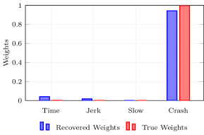
Figure 1: Gridworld experiment with known policy parameters. The learner is using G(PO)MDP algorithm. From left the expected discounted return and the norm difference between the real weights and the recovered ones with one learning step; the same measures with fixed batch size (555 trajectories with length 202020). The performance of the observers are evaluated on the learner’s reward weights. Results are averaged over 20 runs. 98%percent9898\% c.i as shaded area.

This section is devoted to the experimental evaluation of LOGEL. The algorithm LOGEL is compared to the state-of-the-art baseline Learner From a Learner (LfL)  [17] in a gridworld navigation task and in two MuJoCo environments. More details on the experiments are in Appendix B.1.

7.1 Gridworld
Refer to caption
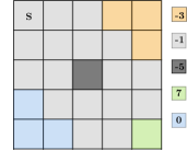
Figure 2: Gridworld environment: every area has a different reward weight. In the green area the agent is reset to the starting state.

The first set of experiments aims at evaluating the performance of LOGEL in a discrete Gridworld environment. The gridworld, represented in Figure 2, is composed of five regions with a different reward for each area. The agent starts from the cell (1,1)11(1,1) and when she reaches the green state, then returns to the starting state. The reward feature space is composed of the one-hot encoding of five areas: the orange, the light grey, the dark grey, the blue, and the green. The learner weights for the areas are (3,1,5,7,0)31570(-3,-1,-5,7,0) respectively.

Refer to caption
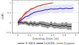
Figure 3: Gridworld experiment with estimated policy parameters and four learner: from left QLearning, G(PO)MDP, SPI, SVI. The green line is the LfL observer and the blue one is the LOGEL observer. The performance of the observers are evaluated on the learner’s reward weights. Results are everaged over 20 runs. 98%percent9898\% c.i as shaded area.

As a first experiment, we want to verify in practice the theoretical finding exposed in Section 4. In this experiment, the learner uses a Boltzmann policy and she is learning with the G(PO)MDP policy gradient algorithm. The observer has access to the true policy parameters of the learner. Figure 1 shows the performance of LOGEL in two settings: a single learning step and increasing batch size (555,101010,202020,303030,404040,505050); a fixed batch size (batch size 555 and trajectory length 202020) and an increasing number of learning steps (222, 444, 666, 888, 101010). The figure shows the expected discounted return (evaluated in closed form) and the difference in norm between the learner’s weights and the recovered weights 111To perform this comparison, we normalize the recovered weights and the learner’s weights. We note that, as explained in Theorem 4.2, with a more accurate gradient estimate, the observer succeeds in recovering the reward weights by observing even just one learning step. On the other hand, as we can deduce from Theorem 4.2, if we have a noisy estimation of the gradient, with multiple learning steps, the observer succeeds in recovering the learner’s weights. It is interesting to notice that, from this experiment, it seems that the bias component, which does not vanish as the learning steps increase (see Theorem 4.2), does not affect the correctness of the recovered weights.

In the second experiment we consider four different learners using: QLearning [34], G(PO)MDP, Soft policy improvement (SPI) [17] and Soft Value Iteration (SVI) [14] 222In Appendix B.1 the learning process of each learning agent is shown.. For this experiment we compare the performance of LOGEL and LfL [17]. In Figure 3 we can notice as LOGEL succeeds in recovering the learner’s reward weights even with learner algorithms other than gradient-based ones. Instead, LfL does not recover the reward weights of the G(PO)MDP learner and needs more learning steps than LOGEL to learn the reward weights when Q-learning learner and SVI are observed.
Refer to caption
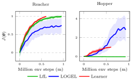
Figure 4: From the left, the Reacher and the Hopper MuJoCo environments. The red line is the performance of the learner during 202020 learning steps. The observers, LfL and LOGEL, observe the trajectories of the last 101010 learning steps. The performance of the observers are evaluated on the learner’s reward weights. Scores are normalized setting to 00 the first return of the learner and to 111 the last one. The results are averaged over 101010 runs. 98%percent9898\% c.i. are shown as shaded areas.

7.2 MuJoCo environments

In the second set of experiments, we show the ability of LOGEL to infer the reward weights in more complex and continuous environments. We use two environments from the MuJoCo control suite [6]: Hopper and Reacher. As in [17], the learner is trained using Policy Proximal Optimization (PPO) [30], with 161616 parallel agents for each learning step. For each step, the length of the trajectories is 200020002000. Then we use LOGEL or LfL to recover the reward parameters. In the end, the observer is trained with the recovered weights using PPO and the performances are evaluated on the learner’s weights, starting from the same initial policy of the learner for a fair comparison. The scores are normalized by setting to 111 the score of the last observed learner policy and to 00 the score of the initial one. In both environments, the observer learns using the learning steps from 101010 to 202020 as the first learning steps are too noisy. The reward function of LfL is the same as the one used in the original paper, where the reward function is a neural network equal to the one used for the learner’s policy. Instead, for LOGEL we used linear reward functions derived from state and action features. The reward for the Reacher environment is a 262626-grid radial basis function that describes the distance between the agent and the goal, plus the 2-norm squared of the action. In the Hopper environment, instead, the reward features are the distance between the previous and the current position and the 2-norm squared of the action.

The results are shown in Figure 4, where we reported results averaged over 101010 runs. We can notice that LOGEL succeeds in identifying a good reward function in both environments, although in the Reacher environment the recovered reward function causes slower learning. Instead, LfL fails to recover an effective reward function for the Hopper environment [17].

8 Conclusions

In this paper we propose a novel algorithm, LOGEL, for the “Learning from a Learner Inverse Reinforcement Learning” setting. The proposed method relies on the assumption that the learner updates her policy along the direction of the gradient of the expected discounted return. We provide some finite-sample bounds on the algorithm performance in recovering the reward weights when the observer observes the learner’s policy parameters and when the observer observes only the learner’s trajectories. Finally, we tested LOGEL on a discrete gridworld environment and on two MuJoCo continuous environments, comparing the algorithm with the state-of-the-art baseline [17]. As future work, we plan to extend the work to account for the uncertainty in estimating both the policy parameters and the gradient.

Broader impact

In this paper, we focus on the Inverse Reinforcement Learning [2, 15, 3, 21] task from a Learning Agent [17]. The first motivation to study Inverse Reinforcement Learning algorithms is to overcome the difficulties that can arise in specifying the reward function from human and animal behavior. Sometimes, in fact, it is easier to infer human intentions by observing their behaviors than to design a reward function by hand. An example is helicopter flight control [1], in which we can observe a helicopter operator and through IRL a reward function is inferred to teach a physical remote-controlled helicopter. Another example is to predict the behavior of a real agent as route prediction tasks of taxis [40, 41] or anticipation of pedestrian interactions [12] or energy-efficient driving [37]. However, in many cases the agents are not really experts and on the other hand only expert demonstrations can not show their intention to avoid dangerous situations. We want to point out that learning what the agent wants to avoid because harmful is as important as learning his intentions.

The possible outcomes of this research are the same as those of Inverse Reinforcement Learning mentioned above, avoiding the constraint that the agent has to be an expert. In future work, we will study how to apply the proposed algorithm in order to infer the pilot’s intentions when they learn a new circuit.

A relevant possible complication of using IRL is the error on the reward feature engineering which can lead to errors in understanding the agent’s intentions. In application such as autonomous driving, errors in the reward function can cause dangerous situations. For this reason, the verification through simulated environment of the effectiveness of the retrieve rewards is quite important.

References

  • [1] Pieter Abbeel, Adam Coates, Morgan Quigley, and Andrew Y Ng. An application of reinforcement learning to aerobatic helicopter flight. In Advances in neural information processing systems, pages 1–8, 2007.
  • [2] Pieter Abbeel and Andrew Y Ng. Apprenticeship learning via inverse reinforcement learning. In Proceedings of the twenty-first international conference on Machine learning, page 1, 2004.
  • [3] Brenna D Argall, Sonia Chernova, Manuela Veloso, and Brett Browning. A survey of robot learning from demonstration. Robotics and autonomous systems, 57(5):469–483, 2009.
  • [4] Ashwin Balakrishna, Brijen Thananjeyan, Jonathan Lee, Felix Li, Arsh Zahed, Joseph E. Gonzalez, and Ken Goldberg. On-policy robot imitation learning from a converging supervisor. In Leslie Pack Kaelbling, Danica Kragic, and Komei Sugiura, editors, 3rd Annual Conference on Robot Learning, CoRL 2019, Osaka, Japan, October 30 - November 1, 2019, Proceedings, volume 100 of Proceedings of Machine Learning Research, pages 24–41. PMLR, 2019.
  • [5] Jonathan Baxter and Peter L Bartlett. Infinite-horizon policy-gradient estimation. Journal of Artificial Intelligence Research, 15:319–350, 2001.
  • [6] Greg Brockman, Vicki Cheung, Ludwig Pettersson, Jonas Schneider, John Schulman, Jie Tang, and Wojciech Zaremba. Openai gym. CoRR, abs/1606.01540, 2016.
  • [7] Daniel Brown, Wonjoon Goo, Prabhat Nagarajan, and Scott Niekum. Extrapolating beyond suboptimal demonstrations via inverse reinforcement learning from observations. In International Conference on Machine Learning, pages 783–792, 2019.
  • [8] George Casella and Roger L Berger. Statistical inference, volume 2. Duxbury Pacific Grove, CA, 2002.
  • [9] Pablo Samuel Castro, Shijian Li, and Daqing Zhang. Inverse reinforcement learning with multiple ranked experts. arXiv preprint arXiv:1907.13411, 2019.
  • [10] Yudong Chen and Constantine Caramanis. Noisy and missing data regression: Distribution-oblivious support recovery. In International Conference on Machine Learning, pages 383–391, 2013.
  • [11] Paul F Christiano, Jan Leike, Tom Brown, Miljan Martic, Shane Legg, and Dario Amodei. Deep reinforcement learning from human preferences. In Advances in Neural Information Processing Systems, pages 4299–4307, 2017.
  • [12] Shu-Yun Chung and Han-Pang Huang. A mobile robot that understands pedestrian spatial behaviors. In 2010 IEEE/RSJ International Conference on Intelligent Robots and Systems, pages 5861–5866. IEEE, 2010.
  • [13] Vineet Goyal and Julien Grand-Clement. A first-order approach to accelerated value iteration. arXiv preprint arXiv:1905.09963, 2019.
  • [14] Tuomas Haarnoja, Aurick Zhou, Pieter Abbeel, and Sergey Levine. Soft actor-critic: Off-policy maximum entropy deep reinforcement learning with a stochastic actor. arXiv preprint arXiv:1801.01290, 2018.
  • [15] Ahmed Hussein, Mohamed Medhat Gaber, Eyad Elyan, and Chrisina Jayne. Imitation learning: A survey of learning methods. ACM Computing Surveys (CSUR), 50(2):21, 2017.
  • [16] Borja Ibarz, Jan Leike, Tobias Pohlen, Geoffrey Irving, Shane Legg, and Dario Amodei. Reward learning from human preferences and demonstrations in atari. In Advances in Neural Information Processing Systems, pages 8011–8023, 2018.
  • [17] Alexis Jacq, Matthieu Geist, Ana Paiva, and Olivier Pietquin. Learning from a learner. In Kamalika Chaudhuri and Ruslan Salakhutdinov, editors, Proceedings of the 36th International Conference on Machine Learning, volume 97 of Proceedings of Machine Learning Research, pages 2990–2999, Long Beach, California, USA, 09–15 Jun 2019. PMLR.
  • [18] Brian McWilliams, Gabriel Krummenacher, Mario Lucic, and Joachim M Buhmann. Fast and robust least squares estimation in corrupted linear models. In Advances in Neural Information Processing Systems, pages 415–423, 2014.
  • [19] Alberto Maria Metelli, Matteo Pirotta, and Marcello Restelli. Compatible reward inverse reinforcement learning. In Advances in Neural Information Processing Systems, pages 2050–2059, 2017.
  • [20] Andrew Y. Ng and Stuart J. Russell. Algorithms for inverse reinforcement learning. In Proceedings of the Seventeenth International Conference on Machine Learning (ICML 2000), Stanford University, Stanford, CA, USA, June 29 - July 2, 2000, pages 663–670. Morgan Kaufmann, 2000.
  • [21] Takayuki Osa, Joni Pajarinen, Gerhard Neumann, J. Andrew Bagnell, Pieter Abbeel, and Jan Peters. An algorithmic perspective on imitation learning. Foundations and Trends in Robotics, 7(1-2):1–179, 2018.
  • [22] Jan Peters and Stefan Schaal. Policy gradient methods for robotics. In 2006 IEEE/RSJ International Conference on Intelligent Robots and Systems, pages 2219–2225. IEEE, 2006.
  • [23] Jan Peters and Stefan Schaal. Reinforcement learning of motor skills with policy gradients. Neural networks, 21(4):682–697, 2008.
  • [24] Matteo Pirotta and Marcello Restelli. Inverse reinforcement learning through policy gradient minimization. In Dale Schuurmans and Michael P. Wellman, editors, Proceedings of the Thirtieth AAAI Conference on Artificial Intelligence, February 12-17, 2016, Phoenix, Arizona, USA, pages 1993–1999. AAAI Press, 2016.
  • [25] Matteo Pirotta, Marcello Restelli, and Luca Bascetta. Adaptive step-size for policy gradient methods. In Advances in Neural Information Processing Systems, pages 1394–1402, 2013.
  • [26] Martin L. Puterman. Markov Decision Processes: Discrete Stochastic Dynamic Programming. John Wiley & Sons, Inc., New York, NY, USA, 1994.
  • [27] Neil Rabinowitz, Frank Perbet, Francis Song, Chiyuan Zhang, SM Ali Eslami, and Matthew Botvinick. Machine theory of mind. In International Conference on Machine Learning, pages 4218–4227, 2018.
  • [28] Philippe Rigollet. High-dimensional statistics. spring 2015. Massachusetts Institute of Technology: MIT OpenCourseWare, 2015.
  • [29] John Schulman, Xi Chen, and Pieter Abbeel. Equivalence between policy gradients and soft q-learning. arXiv preprint arXiv:1704.06440, 2017.
  • [30] John Schulman, Filip Wolski, Prafulla Dhariwal, Alec Radford, and Oleg Klimov. Proximal policy optimization algorithms. arXiv preprint arXiv:1707.06347, 2017.
  • [31] Hanan Shteingart and Yonatan Loewenstein. Reinforcement learning and human behavior. Current Opinion in Neurobiology, 25:93–98, 2014.
  • [32] Michael Shum, Max Kleiman-Weiner, Michael L Littman, and Joshua B Tenenbaum. Theory of minds: Understanding behavior in groups through inverse planning. In Proceedings of the AAAI Conference on Artificial Intelligence, volume 33, pages 6163–6170, 2019.
  • [33] Vladimir Spokoiny et al. Parametric estimation. finite sample theory. The Annals of Statistics, 40(6):2877–2909, 2012.
  • [34] Richard S. Sutton and Andrew G. Barto. Reinforcement Learning: An Introduction. A Bradford book. Bradford Book, 1998.
  • [35] Richard S Sutton, David A McAllester, Satinder P Singh, and Yishay Mansour. Policy gradient methods for reinforcement learning with function approximation. In Advances in Neural Information Processing Systems, pages 1057–1063, 2000.
  • [36] Paul Tseng. Convergence of a block coordinate descent method for nondifferentiable minimization. Journal of optimization theory and applications, 109(3):475–494, 2001.
  • [37] Adam Vogel, Deepak Ramachandran, Rakesh Gupta, and Antoine Raux. Improving hybrid vehicle fuel efficiency using inverse reinforcement learning. In Twenty-Sixth AAAI Conference on Artificial Intelligence, 2012.
  • [38] Perke Wedin. Perturbation theory for pseudo-inverses. BIT Numerical Mathematics, 13(2):217–232, 1973.
  • [39] Ronald J Williams. Simple statistical gradient-following algorithms for connectionist reinforcement learning. Machine learning, 8(3-4):229–256, 1992.
  • [40] Brian D. Ziebart, Andrew L. Maas, J. Andrew Bagnell, and Anind K. Dey. Maximum entropy inverse reinforcement learning. In Dieter Fox and Carla P. Gomes, editors, Proceedings of the Twenty-Third AAAI Conference on Artificial Intelligence, AAAI 2008, Chicago, Illinois, USA, July 13-17, 2008, pages 1433–1438. AAAI Press, 2008.
  • [41] Brian D Ziebart, Andrew L Maas, Anind K Dey, and J Andrew Bagnell. Navigate like a cabbie: Probabilistic reasoning from observed context-aware behavior. In Proceedings of the 10th international conference on Ubiquitous computing, pages 322–331, 2008.

Appendix A Proofs and derivations

We start the proofs given some introduction on Pertubation on Least Square problems and on Least Square problems with fixed design. Then we report the proofs and derivations for the results of Sections 4 and 5. For the rest of this section we assume that:

  • 𝝎L,𝝎^qsuperscript𝝎𝐿^𝝎superscript𝑞\bm{\omega}^{L},\widehat{\bm{\omega}}\in\mathbb{R}^{q},

  • 𝜽L,𝜽^dsuperscript𝜽𝐿^𝜽superscript𝑑\bm{\theta}^{L},\widehat{\bm{\theta}}\in\mathbb{R}^{d}.

We define with 𝝎Lsuperscript𝝎𝐿\bm{\omega}^{L} (𝜽Lsuperscript𝜽𝐿\bm{\theta}^{L}) the reward (policy) parameters of the learner, and with 𝝎^^𝝎\widehat{\bm{\omega}} (𝜽^^𝜽\widehat{\bm{\theta}}) the reward (policy) parameters recovered by the observer.

A.1 Preliminaries

Definition A.1.

The condition number of a matrix 𝐀Rm×q𝐀superscript𝑅𝑚𝑞\bm{\mathbf{A}}\in R^{m\times q} 𝐀0𝐀0\bm{\mathbf{A}}\neq 0 is:

κ=𝐀2𝐀+2=σ1σr,𝜅subscriptnorm𝐀2subscriptnormsuperscript𝐀2subscript𝜎1subscript𝜎𝑟\kappa=\left\|\bm{\mathbf{A}}\right\|_{2}\left\|\bm{\mathbf{A}}^{+}\right\|_{2}=\frac{\sigma_{1}}{\sigma_{r}},

where 0 < r = rank(𝐀𝐀\bm{\mathbf{A}}) min(m,q)absent𝑚𝑞\leq\min(m,q), and σ1σr>0subscript𝜎1subscript𝜎𝑟0\sigma_{1}\geq\cdots\geq\sigma_{r}>0 are the nonzero singular values of 𝐀𝐀\bm{\mathbf{A}}.

A least-squares problem is defined as:

minx𝐀xb2,subscript𝑥subscriptnorm𝐀𝑥𝑏2\min_{x}\left\|\bm{\mathbf{A}}x-b\right\|_{2}, (10)

where the solution is x=𝐀+b𝑥superscript𝐀𝑏x=\bm{\mathbf{A}}^{+}b. We denote with 𝐀+superscript𝐀\bm{\mathbf{A}}^{+} the pseudoinverse of 𝐀𝐀\bm{\mathbf{A}}, the perturbed 𝐀𝐀\bm{\mathbf{A}} as 𝐀^=𝐀+δ𝐀^𝐀𝐀𝛿𝐀\widehat{\bm{\mathbf{A}}}=\bm{\mathbf{A}}+\delta\bm{\mathbf{A}} and the pertubed b^=b+δb^𝑏𝑏𝛿𝑏\hat{b}=b+\delta b and the perturbed solution x^=𝐀^+b^=x+δx^𝑥superscript^𝐀^𝑏𝑥𝛿𝑥\widehat{x}=\widehat{\bm{\mathbf{A}}}^{+}\hat{b}=x+\delta x. Finally, we denote with 𝐀Hsuperscript𝐀𝐻\bm{\mathbf{A}}^{H} the adjoint of the matrix 𝐀𝐀\bm{\mathbf{A}}.

We define as χ=δ𝐀2𝐀2𝜒subscriptnorm𝛿𝐀2subscriptnorm𝐀2\chi=\frac{\left\|\delta\bm{\mathbf{A}}\right\|_{2}}{\left\|\bm{\mathbf{A}}\right\|_{2}} and y=𝐀+Hx𝑦superscript𝐀𝐻𝑥y=\bm{\mathbf{A}}^{+H}x.

Lemma A.1 (Perturbation on Least Square Problems [38]).

Assume that rank(𝐀+δ𝐀𝐀𝛿𝐀\bm{\mathbf{A}}+\delta\bm{\mathbf{A}}) = rank(𝐀𝐀\bm{\mathbf{A}}) and χκ<1𝜒𝜅1\chi\kappa<1 then:

xx^2κ(1χκ)𝐀2(χx2𝐀2+χκr2+δb2)+χy2𝐀2.subscriptnorm𝑥^𝑥2𝜅1𝜒𝜅subscriptnorm𝐀2𝜒subscriptnorm𝑥2subscriptnorm𝐀2𝜒𝜅subscriptnorm𝑟2subscriptnorm𝛿𝑏2𝜒subscriptnorm𝑦2subscriptnorm𝐀2\left\|x-\hat{x}\right\|_{2}\leq\frac{\kappa}{(1-\chi\kappa)\left\|\bm{\mathbf{A}}\right\|_{2}}(\chi\left\|x\right\|_{2}\left\|\bm{\mathbf{A}}\right\|_{2}+\chi\kappa\left\|r\right\|_{2}+\left\|\delta b\right\|_{2})+\chi\left\|y\right\|_{2}\left\|\bm{\mathbf{A}}\right\|_{2}. (11)
Proof.

The proof can be find in [38]. ∎

We adapt the lemma 6 in [10] to our context where 𝝎^^𝝎\widehat{\bm{\omega}} are the reward weights recovered with lemma 4.1.

Lemma A.2 (From lemma 6 in [10]).

Let Σ=(𝛉𝛙^T𝛉𝛙^)Σsuperscript^subscript𝛉𝛙𝑇^subscript𝛉𝛙\Sigma=(\widehat{\nabla_{\bm{\theta}}\bm{\psi}}^{T}\widehat{\nabla_{\bm{\theta}}\bm{\psi}}) and suppose the following strong convexity condition holds: λmin(Σ)λ>0subscript𝜆Σ𝜆0\lambda_{\min}(\Sigma)\geq\lambda>0. Then the estimation error satisfies:

𝝎^𝝎L2O(1λ𝜽𝝍TΔΣ𝝎L2).subscriptnorm^𝝎superscript𝝎𝐿2𝑂1𝜆subscriptnormsubscript𝜽superscript𝝍𝑇ΔΣsuperscript𝝎𝐿2\left\|\widehat{\bm{\omega}}-\bm{\omega}^{L}\right\|_{2}\leq O\left(\frac{1}{\lambda}\left\|\nabla_{\bm{\theta}}\bm{\psi}^{T}\Delta-\Sigma\bm{\omega}^{L}\right\|_{2}\right).
Lemma A.3 (Revised from lemma 11 in [18]).

Suppose Xm×q𝑋superscript𝑚𝑞X\in\mathbb{R}^{m\times q} and Wn×M𝑊superscript𝑛𝑀W\in\mathbb{R}^{n\times M} are zero-mean sub-gaussian matrices with parameters (1nΣx,1nσx2),(1nΣw,1nσw2)1𝑛subscriptΣ𝑥1𝑛subscriptsuperscript𝜎2𝑥1𝑛subscriptΣ𝑤1𝑛subscriptsuperscript𝜎2𝑤(\frac{1}{n}\Sigma_{x},\frac{1}{n}\sigma^{2}_{x}),(\frac{1}{n}\Sigma_{w},\frac{1}{n}\sigma^{2}_{w}) respectively. Then for any fixed vectors v1,v2subscript𝑣1subscript𝑣2v_{1},v_{2}, we have:

P[|v1T(WTX𝔼[WTW])v2|tv12v22]3exp(cnmin{t2σx2σw2,tσxσw}),Pdelimited-[]superscriptsubscript𝑣1𝑇superscript𝑊𝑇𝑋𝔼superscript𝑊𝑇𝑊subscript𝑣2𝑡subscriptnormsubscript𝑣12subscriptnormsubscript𝑣223𝑒𝑥𝑝𝑐𝑛superscript𝑡2superscriptsubscript𝜎𝑥2superscriptsubscript𝜎𝑤2𝑡subscript𝜎𝑥subscript𝜎𝑤\text{P}[|v_{1}^{T}(W^{T}X-\operatorname*{\mathbb{E}}[W^{T}W])v_{2}|\geq t\left\|v_{1}\right\|_{2}\left\|v_{2}\right\|_{2}]\leq 3exp\left(-cn\min\left\{\frac{t^{2}}{\sigma_{x}^{2}\sigma_{w}^{2}},\frac{t}{\sigma_{x}\sigma_{w}}\right\}\right),

in particular if nlogpgreater-than-or-equivalent-to𝑛𝑝n\gtrsim\log p we have that:

|v1T(WTX𝔼[WTW])v2|σxσwv12v22logpn.superscriptsubscript𝑣1𝑇superscript𝑊𝑇𝑋𝔼superscript𝑊𝑇𝑊subscript𝑣2subscript𝜎𝑥subscript𝜎𝑤subscriptnormsubscript𝑣12subscriptnormsubscript𝑣22𝑝𝑛|v_{1}^{T}(W^{T}X-\operatorname*{\mathbb{E}}[W^{T}W])v_{2}|\leq\sigma_{x}\sigma_{w}\left\|v_{1}\right\|_{2}\left\|v_{2}\right\|_{2}\sqrt{\frac{\log p}{n}}.

Setting v1subscript𝑣1v_{1} to be the first standard basis vector and using a union bound over j=1,,p𝑗1𝑝j=1,\cdots,p we have:

(WTX𝔼[WTX])vσxσwv2logpn,subscriptnormsuperscript𝑊𝑇𝑋𝔼superscript𝑊𝑇𝑋𝑣subscript𝜎𝑥subscript𝜎𝑤subscriptnorm𝑣2𝑝𝑛\left\|(W^{T}X-\operatorname*{\mathbb{E}}[W^{T}X])v\right\|_{\infty}\leq\sigma_{x}\sigma_{w}\left\|v\right\|_{2}\sqrt{\frac{\log p}{n}},

with probability 1c1exp(c2logp)1subscript𝑐1𝑒𝑥𝑝subscript𝑐2𝑝1-c_{1}exp(-c_{2}\log p) where c1,c2subscript𝑐1subscript𝑐2c_{1},c_{2} are positive constants which are independent from σx,σw,n,psubscript𝜎𝑥subscript𝜎𝑤𝑛𝑝\sigma_{x},\sigma_{w},n,p.

Theorem A.1 (from Chapter 2 [28]).

Assume that the least-squares model:

minx𝐀xb+ϵsubscript𝑥norm𝐀𝑥𝑏italic-ϵ\min_{x}\left\|\bm{\mathbf{A}}x-b+\epsilon\right\|

holds where ϵsubGn(σ2)similar-toitalic-ϵsubGnsuperscript𝜎2\epsilon\sim\text{subGn}(\sigma^{2}). Then, for any δ>0𝛿0\delta>0, with probability 1δ1𝛿1-\delta it holds:

xx^2σr+log(1δ)nσmin,subscriptnorm𝑥^𝑥2𝜎𝑟1𝛿𝑛subscript𝜎\left\|x-\hat{x}\right\|_{2}\leq\sigma\sqrt{\frac{r+\log(\frac{1}{\delta})}{n\sigma_{\min}}},

where σmin=𝐀T𝐀nsubscript𝜎superscript𝐀𝑇𝐀𝑛\sigma_{\min}=\frac{\bm{\mathbf{A}}^{T}\bm{\mathbf{A}}}{n} is the minimum singular value of 𝐀T𝐀superscript𝐀𝑇𝐀\bm{\mathbf{A}}^{T}\bm{\mathbf{A}} and r𝑟r is the rank(𝐀T𝐀superscript𝐀𝑇𝐀\bm{\mathbf{A}}^{T}\bm{\mathbf{A}}).

A.2 Proofs and derivation of Section 4

In this section we give the proofs and derivations of the theorems in Section 4.

First, we will provide a finite sample analysis on the difference in norm between the reward vector of the learner 𝝎Lsuperscript𝝎𝐿\bm{\omega}^{L} and the reward vector recoverd using (5), with a single learning step. This result was omitted in the main paper as we can see this as a special case of Theorem 4.2, but with a different technique. We add it here as it provides a first insight on how, having enough demonstrations, we can recover the correct weights. In the demonstration, without loss of generality, we assume that the learning rate is 111.

Lemma A.4.

Let 𝛉𝛙subscript𝛉𝛙\nabla_{\bm{\theta}}\bm{\psi} be the real Jacobian and 𝛉𝛙^^subscript𝛉𝛙\widehat{\nabla_{\bm{\theta}}\bm{\psi}} the estimated Jacobian from n𝑛n trajectories {τ1,,τn}subscript𝜏1subscript𝜏𝑛\{\tau_{1},\cdots,\tau_{n}\}. Assume that 𝛉ψ^^subscript𝛉𝜓\widehat{\nabla_{\bm{\theta}}\psi} is uniformly bounded by M𝑀M. Then with probability 1δ1𝛿1-\delta

𝜽ψ^𝜽ψ2Mqdlog(2δ)2n.subscriptnorm^subscript𝜽𝜓subscript𝜽𝜓2𝑀𝑞𝑑2𝛿2𝑛\left\|\widehat{\nabla_{\bm{\theta}}\psi}-\nabla_{\bm{\theta}}\psi\right\|_{2}\leq M\sqrt{qd}\sqrt{\frac{\log(\frac{2}{\delta})}{2n}}.
Proof.

We use Hoeffding’s inequality:

P[𝜽ψ^𝜽ψ2t]P[qd𝜽ψ^𝜽ψt]2exp(2t2ndqM2)Pdelimited-[]subscriptnorm^subscript𝜽𝜓subscript𝜽𝜓2𝑡Pdelimited-[]𝑞𝑑subscriptnorm^subscript𝜽𝜓subscript𝜽𝜓𝑡22superscript𝑡2𝑛𝑑𝑞superscript𝑀2\displaystyle\text{P}\left[\left\|\widehat{\nabla_{\bm{\theta}}\psi}-\nabla_{\bm{\theta}}\psi\right\|_{2}\geq t\right]\leq\text{P}\left[\sqrt{qd}\left\|\widehat{\nabla_{\bm{\theta}}\psi}-\nabla_{\bm{\theta}}\psi\right\|_{\infty}\geq t\right]\leq 2\exp\left(\frac{-2t^{2}n}{dqM^{2}}\right)

The result follows by setting δ=2exp(2t2ndqM2)𝛿22superscript𝑡2𝑛𝑑𝑞superscript𝑀2\delta=2\exp\left(\frac{-2t^{2}n}{dqM^{2}}\right). ∎

{thm}

[] Let 𝜽ψsubscript𝜽𝜓\nabla_{\bm{\theta}}\psi be the real Jacobian and 𝜽ψ^^subscript𝜽𝜓\widehat{\nabla_{\bm{\theta}}\psi} the estimated Jacobian from n𝑛n trajectories {τ1,,τn}subscript𝜏1subscript𝜏𝑛\{\tau_{1},\cdots,\tau_{n}\}. Assume that 𝜽ψ^^subscript𝜽𝜓\widehat{\nabla_{\bm{\theta}}\psi} is uniformly bounded by M𝑀M, rank(𝜽𝝍^)=rank(𝜽𝝍)𝑟𝑎𝑛𝑘^subscript𝜽𝝍𝑟𝑎𝑛𝑘subscript𝜽𝝍rank(\widehat{\nabla_{\bm{\theta}}\bm{\psi}})=rank(\nabla_{\bm{\theta}}\bm{\psi}) and 𝜽𝝍^𝜽𝝍2κ𝜽𝝍<𝜽𝝍2subscriptnorm^subscript𝜽𝝍subscript𝜽𝝍2subscript𝜅subscript𝜽𝝍subscriptnormsubscript𝜽𝝍2\left\|\widehat{\nabla_{\bm{\theta}}\bm{\psi}}-\nabla_{\bm{\theta}}\bm{\psi}\right\|_{2}\cdot\kappa_{\nabla_{\bm{\theta}}\bm{\psi}}<\left\|\nabla_{\bm{\theta}}\bm{\psi}\right\|_{2}. Then with probability 1δ1𝛿1-\delta:

𝝎L𝝎^2Mqdlog(2δ)2n(κ𝜽𝝍𝝎L2c𝜽𝝍2+y2),subscriptnormsuperscript𝝎𝐿^𝝎2𝑀𝑞𝑑2𝛿2𝑛subscript𝜅subscript𝜽𝝍subscriptnormsuperscript𝝎𝐿2𝑐subscriptnormsubscript𝜽𝝍2subscriptnorm𝑦2\left\|\bm{\omega}^{L}-\hat{\bm{\omega}}\right\|_{2}\leq M\sqrt{qd}\sqrt{\frac{\log(\frac{2}{\delta})}{2n}}\left(\frac{\kappa_{\nabla_{\bm{\theta}}\bm{\psi}}\left\|\bm{\omega}^{L}\right\|_{2}}{c\left\|\nabla_{\bm{\theta}}\bm{\psi}\right\|_{2}}+\left\|y\right\|_{2}\right), (12)

where ωLsuperscript𝜔𝐿\omega^{L} are the real reward parameters and ω^^𝜔\hat{\omega} are the parameters recovered with Equation (5), c=1𝜽𝝍^𝜽𝝍2𝜽𝝍2κ𝜽𝝍>0𝑐1subscriptnorm^subscript𝜽𝝍subscript𝜽𝝍2subscriptnormsubscript𝜽𝝍2subscript𝜅subscript𝜽𝝍0c=1-\frac{\left\|\widehat{\nabla_{\bm{\theta}}\bm{\psi}}-\nabla_{\bm{\theta}}\bm{\psi}\right\|_{2}}{\left\|\nabla_{\bm{\theta}}\bm{\psi}\right\|_{2}}\kappa_{\nabla_{\bm{\theta}}\bm{\psi}}>0, and y=𝜽𝝍+H𝝎𝑦subscript𝜽superscript𝝍𝐻𝝎y=\nabla_{\bm{\theta}}\bm{\psi}^{+H}\bm{\omega}.

Proof.

We need to bound the difference in norm between 𝝎Lsuperscript𝝎𝐿\bm{\omega}^{L} and 𝝎^^𝝎\widehat{\bm{\omega}} that are the true parameters and the parameters that we recovered solving the minimization problem (4). 𝝎L𝝎^2subscriptnormsuperscript𝝎𝐿^𝝎2\displaystyle\left\|\bm{\omega}^{L}-\widehat{\bm{\omega}}\right\|_{2} (13) κ(1κδ𝜽𝝍2𝜽𝝍2)𝜽𝝍2(δ𝜽𝝍2𝜽𝝍2𝝎L2𝜽𝝍2)+δ𝜽𝝍2𝜽𝝍2y2𝜽𝝍2absent𝜅1𝜅subscriptnorm𝛿subscript𝜽𝝍2subscriptnormsubscript𝜽𝝍2subscriptnormsubscript𝜽𝝍2subscriptnorm𝛿subscript𝜽𝝍2subscriptnormsubscript𝜽𝝍2subscriptnormsuperscript𝝎𝐿2subscriptnormsubscript𝜽𝝍2subscriptnorm𝛿subscript𝜽𝝍2subscriptnormsubscript𝜽𝝍2subscriptnorm𝑦2subscriptnormsubscript𝜽𝝍2\displaystyle\leq\frac{\kappa}{\left(1-\kappa\frac{\left\|\delta\nabla_{\bm{\theta}}\bm{\psi}\right\|_{2}}{\left\|\nabla_{\bm{\theta}}\bm{\psi}\right\|_{2}}\right)\left\|\nabla_{\bm{\theta}}\bm{\psi}\right\|_{2}}\left(\ \frac{\left\|\delta\nabla_{\bm{\theta}}\bm{\psi}\right\|_{2}}{\left\|\nabla_{\bm{\theta}}\bm{\psi}\right\|_{2}}\left\|\bm{\omega}^{L}\right\|_{2}\left\|\nabla_{\bm{\theta}}\bm{\psi}\right\|_{2}\right)+\frac{\left\|\delta\nabla_{\bm{\theta}}\bm{\psi}\right\|_{2}}{\left\|\nabla_{\bm{\theta}}\bm{\psi}\right\|_{2}}\left\|y\right\|_{2}\left\|\nabla_{\bm{\theta}}\bm{\psi}\right\|_{2} (14) κc𝜽𝝍2(δ𝜽𝝍2𝜽𝝍2𝝎L2𝜽𝝍2)+δ𝜽𝝍2𝜽𝝍2y2𝜽𝝍2absent𝜅𝑐subscriptnormsubscript𝜽𝝍2subscriptnorm𝛿subscript𝜽𝝍2subscriptnormsubscript𝜽𝝍2subscriptnormsuperscript𝝎𝐿2subscriptnormsubscript𝜽𝝍2subscriptnorm𝛿subscript𝜽𝝍2subscriptnormsubscript𝜽𝝍2subscriptnorm𝑦2subscriptnormsubscript𝜽𝝍2\displaystyle\leq\frac{\kappa}{c\left\|\nabla_{\bm{\theta}}\bm{\psi}\right\|_{2}}\left(\ \frac{\left\|\delta\nabla_{\bm{\theta}}\bm{\psi}\right\|_{2}}{\left\|\nabla_{\bm{\theta}}\bm{\psi}\right\|_{2}}\left\|\bm{\omega}^{L}\right\|_{2}\left\|\nabla_{\bm{\theta}}\bm{\psi}\right\|_{2}\right)+\frac{\left\|\delta\nabla_{\bm{\theta}}\bm{\psi}\right\|_{2}}{\left\|\nabla_{\bm{\theta}}\bm{\psi}\right\|_{2}}\left\|y\right\|_{2}\left\|\nabla_{\bm{\theta}}\bm{\psi}\right\|_{2} (15) =δ𝜽𝝍2(κ𝝎L2c𝜽𝝍2+y2)absentsubscriptnorm𝛿subscript𝜽𝝍2𝜅subscriptnormsuperscript𝝎𝐿2𝑐subscriptnormsubscript𝜽𝝍2subscriptnorm𝑦2\displaystyle=\left\|\delta\nabla_{\bm{\theta}}\bm{\psi}\right\|_{2}\left(\frac{\kappa\left\|\bm{\omega}^{L}\right\|_{2}}{c\left\|\nabla_{\bm{\theta}}\bm{\psi}\right\|_{2}}+\left\|y\right\|_{2}\right) (16) Mqdlog(2δ)2n(κ𝝎L2c𝜽𝝍2+y2),absent𝑀𝑞𝑑2𝛿2𝑛𝜅subscriptnormsuperscript𝝎𝐿2𝑐subscriptnormsubscript𝜽𝝍2subscriptnorm𝑦2\displaystyle\leq M\sqrt{qd}\sqrt{\frac{\log(\frac{2}{\delta})}{2n}}\left(\frac{\kappa\left\|\bm{\omega}^{L}\right\|_{2}}{c\left\|\nabla_{\bm{\theta}}\bm{\psi}\right\|_{2}}+\left\|y\right\|_{2}\right), (17) where line (14) is obtained by using Lemma A.1, lines (15, 16) by rearranging the terms, and line (17) by using Lemma A.4. We can observe that the last term vanishes when the rank(𝜽𝝍subscript𝜽𝝍\nabla_{\bm{\theta}}\bm{\psi})=qabsent𝑞=q (see [38]). ∎

Now we will give the proofs and derivations of Lemmas 4.1 and Theorem 4.2.

See 4.1

Proof.

Taking the derivative of (4) with respect to ω𝜔\omega:

𝝎t=1mΔtαt𝜽𝝍t𝝎22subscript𝝎superscriptsubscript𝑡1𝑚superscriptsubscriptnormsubscriptΔ𝑡subscript𝛼𝑡subscript𝜽subscript𝝍𝑡𝝎22\displaystyle\nabla_{\bm{\omega}}\sum_{t=1}^{m}\left\|\Delta_{t}-\alpha_{t}\nabla_{\bm{\theta}}\bm{\psi}_{t}\bm{\omega}\right\|_{2}^{2} =t=1m𝝎(Δtαt𝜽𝝍t𝝎)T(Δα𝜽𝝍t𝝎)\displaystyle=\sum_{t=1}^{m}\nabla_{\bm{\omega}}(\Delta_{t}-\alpha_{t}\nabla_{\bm{\theta}}\bm{\psi}_{t}\bm{\omega})^{T}(\Delta-\alpha\nabla_{\bm{\theta}}\bm{\psi}_{t}\bm{\omega})
=t=1m𝝎(ΔtTΔt+(α𝜽𝝍t𝝎)T(αt𝜽𝝍t𝝎)2αt𝜽𝝍t𝝎)TΔt)\displaystyle=\sum_{t=1}^{m}\nabla_{\bm{\omega}}(\Delta_{t}^{T}\Delta_{t}+(\alpha\nabla_{\bm{\theta}}\bm{\psi}_{t}\bm{\omega})^{T}(\alpha_{t}\nabla_{\bm{\theta}}\bm{\psi}_{t}\bm{\omega})-2\alpha_{t}\nabla_{\bm{\theta}}\bm{\psi}_{t}\bm{\omega})^{T}\Delta_{t})
=2(t=1mαt2𝜽𝝍tT𝜽𝝍t)𝝎2t=1m(αt𝜽𝝍tTΔt).absent2superscriptsubscript𝑡1𝑚superscriptsubscript𝛼𝑡2subscript𝜽superscriptsubscript𝝍𝑡𝑇subscript𝜽subscript𝝍𝑡𝝎2superscriptsubscript𝑡1𝑚subscript𝛼𝑡subscript𝜽superscriptsubscript𝝍𝑡𝑇subscriptΔ𝑡\displaystyle=2\left(\sum_{t=1}^{m}\alpha_{t}^{2}\nabla_{\bm{\theta}}\bm{\psi}_{t}^{T}\nabla_{\bm{\theta}}\bm{\psi}_{t}\right)\bm{\omega}-2\sum_{t=1}^{m}\left(\alpha_{t}\nabla_{\bm{\theta}}\bm{\psi}_{t}^{T}\Delta_{t}\right).

Taking it equal to zero:

(t=1mαt2𝜽𝝍tT𝜽𝝍t)𝝎t=1m(αt𝜽𝝍tTΔt)=0superscriptsubscript𝑡1𝑚superscriptsubscript𝛼𝑡2subscript𝜽superscriptsubscript𝝍𝑡𝑇subscript𝜽subscript𝝍𝑡𝝎superscriptsubscript𝑡1𝑚subscript𝛼𝑡subscript𝜽superscriptsubscript𝝍𝑡𝑇subscriptΔ𝑡0\displaystyle\left(\sum_{t=1}^{m}\alpha_{t}^{2}\nabla_{\bm{\theta}}\bm{\psi}_{t}^{T}\nabla_{\bm{\theta}}\bm{\psi}_{t}\right)\bm{\omega}-\sum_{t=1}^{m}\left(\alpha_{t}\nabla_{\bm{\theta}}\bm{\psi}_{t}^{T}\Delta_{t}\right)=0
𝝎=(t=1mαt2𝜽𝝍tT𝜽𝝍t)1(t=1mαt𝜽𝝍tTΔt)𝝎superscriptsuperscriptsubscript𝑡1𝑚superscriptsubscript𝛼𝑡2subscript𝜽superscriptsubscript𝝍𝑡𝑇subscript𝜽subscript𝝍𝑡1superscriptsubscript𝑡1𝑚subscript𝛼𝑡subscript𝜽superscriptsubscript𝝍𝑡𝑇subscriptΔ𝑡\displaystyle\bm{\omega}=\left(\sum_{t=1}^{m}\alpha_{t}^{2}\nabla_{\bm{\theta}}\bm{\psi}_{t}^{T}\nabla_{\bm{\theta}}\bm{\psi}_{t}\right)^{-1}\left(\sum_{t=1}^{m}\alpha_{t}\nabla_{\bm{\theta}}\bm{\psi}_{t}^{T}\Delta_{t}\right)

Lemma A.5.

The regularized version of (4) is equal to:

min𝝎t=1mΔtαt𝜽𝝍t𝝎22+λ𝝎22,subscript𝝎superscriptsubscript𝑡1𝑚subscriptsuperscriptnormsubscriptΔ𝑡subscript𝛼𝑡subscript𝜽subscript𝝍𝑡𝝎22𝜆subscriptsuperscriptnorm𝝎22\min_{\bm{\omega}}\sum_{t=1}^{m}\left\|\Delta_{t}-\alpha_{t}\nabla_{\bm{\theta}}\bm{\psi}_{t}\bm{\omega}\right\|^{2}_{2}+\lambda\left\|\bm{\omega}\right\|^{2}_{2},

where λ>0𝜆0\lambda>0. We can solve the regularized problem in closed form:

𝝎=(t=1mαt2𝜽𝝍tT𝜽𝝍t+λ𝐈d)1(t=1mαt𝜽𝝍tTΔt).𝝎superscriptsuperscriptsubscript𝑡1𝑚superscriptsubscript𝛼𝑡2subscript𝜽superscriptsubscript𝝍𝑡𝑇subscript𝜽subscript𝝍𝑡𝜆subscript𝐈𝑑1superscriptsubscript𝑡1𝑚subscript𝛼𝑡subscript𝜽superscriptsubscript𝝍𝑡𝑇subscriptΔ𝑡\bm{\omega}=\left(\sum_{t=1}^{m}\alpha_{t}^{2}\nabla_{\bm{\theta}}\bm{\psi}_{t}^{T}\nabla_{\bm{\theta}}\bm{\psi}_{t}+\lambda\mathbf{I}_{d}\right)^{-1}\left(\sum_{t=1}^{m}\alpha_{t}\nabla_{\bm{\theta}}\bm{\psi}_{t}^{T}\Delta_{t}\right).
Proof.

Taking the derivative respect to ω𝜔\omega:

𝝎t=1mΔtαt𝜽𝝍t𝝎22+λ𝝎22=t=1m𝝎(Δtαt𝜽𝝍t𝝎)T(Δα𝜽𝝍t𝝎)+𝝎λ𝝎T𝝎\displaystyle\nabla_{\bm{\omega}}\sum_{t=1}^{m}\left\|\Delta_{t}-\alpha_{t}\nabla_{\bm{\theta}}\bm{\psi}_{t}\bm{\omega}\right\|_{2}^{2}+\lambda\left\|\bm{\omega}\right\|_{2}^{2}=\sum_{t=1}^{m}\nabla_{\bm{\omega}}(\Delta_{t}-\alpha_{t}\nabla_{\bm{\theta}}\bm{\psi}_{t}\bm{\omega})^{T}(\Delta-\alpha\nabla_{\bm{\theta}}\bm{\psi}_{t}\bm{\omega})+\nabla_{\bm{\omega}}\lambda\bm{\omega}^{T}\bm{\omega}
=t=1m𝝎(ΔtTΔt+(α𝜽𝝍t𝝎)T(αt𝜽𝝍t𝝎)2αt𝜽𝝍t𝝎)TΔt)+2λ𝝎\displaystyle=\sum_{t=1}^{m}\nabla_{\bm{\omega}}(\Delta_{t}^{T}\Delta_{t}+(\alpha\nabla_{\bm{\theta}}\bm{\psi}_{t}\bm{\omega})^{T}(\alpha_{t}\nabla_{\bm{\theta}}\bm{\psi}_{t}\bm{\omega})-2\alpha_{t}\nabla_{\bm{\theta}}\bm{\psi}_{t}\bm{\omega})^{T}\Delta_{t})+2\lambda\bm{\omega}
=2(t=1mαt2𝜽𝝍tT𝜽𝝍t)𝝎2t=1m(αt𝜽𝝍tTΔt)+2λ𝝎.absent2superscriptsubscript𝑡1𝑚superscriptsubscript𝛼𝑡2subscript𝜽superscriptsubscript𝝍𝑡𝑇subscript𝜽subscript𝝍𝑡𝝎2superscriptsubscript𝑡1𝑚subscript𝛼𝑡subscript𝜽superscriptsubscript𝝍𝑡𝑇subscriptΔ𝑡2𝜆𝝎\displaystyle=2\left(\sum_{t=1}^{m}\alpha_{t}^{2}\nabla_{\bm{\theta}}\bm{\psi}_{t}^{T}\nabla_{\bm{\theta}}\bm{\psi}_{t}\right)\bm{\omega}-2\sum_{t=1}^{m}\left(\alpha_{t}\nabla_{\bm{\theta}}\bm{\psi}_{t}^{T}\Delta_{t}\right)+2\lambda\bm{\omega}.

Taking it equal to zero:

(t=1mαt2𝜽𝝍tT𝜽𝝍t+λ𝐈d)𝝎t=1m(αt𝜽𝝍tTΔt)=0superscriptsubscript𝑡1𝑚superscriptsubscript𝛼𝑡2subscript𝜽superscriptsubscript𝝍𝑡𝑇subscript𝜽subscript𝝍𝑡𝜆subscript𝐈𝑑𝝎superscriptsubscript𝑡1𝑚subscript𝛼𝑡subscript𝜽superscriptsubscript𝝍𝑡𝑇subscriptΔ𝑡0\displaystyle\left(\sum_{t=1}^{m}\alpha_{t}^{2}\nabla_{\bm{\theta}}\bm{\psi}_{t}^{T}\nabla_{\bm{\theta}}\bm{\psi}_{t}+\lambda\mathbf{I}_{d}\right)\bm{\omega}-\sum_{t=1}^{m}\left(\alpha_{t}\nabla_{\bm{\theta}}\bm{\psi}_{t}^{T}\Delta_{t}\right)=0
𝝎=(t=1mαt2𝜽𝝍tT𝜽𝝍t+λ𝐈d)1(t=1mαt𝜽𝝍tTΔt).𝝎superscriptsuperscriptsubscript𝑡1𝑚superscriptsubscript𝛼𝑡2subscript𝜽superscriptsubscript𝝍𝑡𝑇subscript𝜽subscript𝝍𝑡𝜆subscript𝐈𝑑1superscriptsubscript𝑡1𝑚subscript𝛼𝑡subscript𝜽superscriptsubscript𝝍𝑡𝑇subscriptΔ𝑡\displaystyle\bm{\omega}=\left(\sum_{t=1}^{m}\alpha_{t}^{2}\nabla_{\bm{\theta}}\bm{\psi}_{t}^{T}\nabla_{\bm{\theta}}\bm{\psi}_{t}+\lambda\mathbf{I}_{d}\right)^{-1}\left(\sum_{t=1}^{m}\alpha_{t}\nabla_{\bm{\theta}}\bm{\psi}_{t}^{T}\Delta_{t}\right).

See 4.2

Proof.

We decompose the estimated Jacobian 𝚿=𝚿+E𝚿𝚿𝐸\bm{\mathbf{\Psi}}=\bm{\mathbf{\Psi}}+E, where E𝐸E is the random variable component caused by the estimation of the 𝜽𝝍subscript𝜽𝝍\nabla_{\bm{\theta}}\bm{\psi}. Since we estimate the jacobians with an unbiased estimator the mean of E𝐸E is 00. We reshape the 𝚿𝚿\bm{\mathbf{\Psi}} and E𝐸E as 𝚿m×dq𝚿superscript𝑚𝑑𝑞\bm{\mathbf{\Psi}}\in\mathbb{R}^{m\times dq} and Em×dq𝐸superscript𝑚𝑑𝑞E\in\mathbb{R}^{m\times dq}. Now E𝐸E, since its mean is 00 and all lines are independent of each other, is a sub-Gaussian matrix with parameters (1mΣE,1mσE)1𝑚subscriptΣ𝐸1𝑚subscript𝜎𝐸(\frac{1}{m}\Sigma_{E},\frac{1}{m}\sigma_{E}). The proof is similar to the proof of Theorem 1 in [18].

(𝚿+E)T(𝚿T𝝎L)(𝚿+E)T(𝚿+E)𝝎L2subscriptnormsuperscript𝚿𝐸𝑇superscript𝚿𝑇superscript𝝎𝐿superscript𝚿𝐸𝑇𝚿𝐸superscript𝝎𝐿2\displaystyle\left\|(\bm{\mathbf{\Psi}}+E)^{T}(\bm{\mathbf{\Psi}}^{T}\bm{\omega}^{L})-(\bm{\mathbf{\Psi}}+E)^{T}(\bm{\mathbf{\Psi}}+E)\bm{\omega}^{L}\right\|_{2}
=𝚿T𝜽𝝍T𝝎+ET𝚿T𝝎L𝚿T𝚿𝝎L𝚿TE𝝎E𝚿T𝝎ETE𝝎L2absentsubscriptnormsuperscript𝚿𝑇subscript𝜽superscript𝝍𝑇superscript𝝎superscript𝐸𝑇superscript𝚿𝑇superscript𝝎𝐿superscript𝚿𝑇𝚿superscript𝝎𝐿superscript𝚿𝑇𝐸superscript𝝎𝐸superscript𝚿𝑇superscript𝝎superscript𝐸𝑇𝐸superscript𝝎𝐿2\displaystyle=\left\|\bm{\mathbf{\Psi}}^{T}\nabla_{\bm{\theta}}\bm{\psi}^{T}\bm{\omega}^{*}+E^{T}\bm{\mathbf{\Psi}}^{T}\bm{\omega}^{L}-\bm{\mathbf{\Psi}}^{T}\bm{\mathbf{\Psi}}\bm{\omega}^{L}-\bm{\mathbf{\Psi}}^{T}E\bm{\omega}^{*}-E\bm{\mathbf{\Psi}}^{T}\bm{\omega}^{*}-E^{T}E\bm{\omega}^{L}\right\|_{2}
=𝚿TE𝝎LETE𝝎L2.absentsubscriptnormsuperscript𝚿𝑇𝐸superscript𝝎𝐿superscript𝐸𝑇𝐸superscript𝝎𝐿2\displaystyle=\left\|-\bm{\mathbf{\Psi}}^{T}E\bm{\omega}^{L}-E^{T}E\bm{\omega}^{L}\right\|_{2}.

Now we bound separately these two terms, using Lemma A.3 as in [18]:

𝚿TE𝝎2subscriptnormsuperscript𝚿𝑇𝐸𝝎2\displaystyle\left\|\bm{\mathbf{\Psi}}^{T}E\bm{\omega}\right\|_{2} 𝚿2σE𝝎L2logdqmabsentsubscriptnorm𝚿2subscript𝜎𝐸subscriptnormsuperscript𝝎𝐿2𝑑𝑞𝑚\displaystyle\leq\left\|\bm{\mathbf{\Psi}}\right\|_{2}\sigma_{E}\left\|\bm{\omega}^{L}\right\|_{2}\sqrt{\frac{\log dq}{m}}
ETE𝝎L2subscriptnormsuperscript𝐸𝑇𝐸superscript𝝎𝐿2\displaystyle\left\|E^{T}E\bm{\omega}^{L}\right\|_{2} =(ETE+σE2𝐈qdσE2𝐈qd)𝝎L2σE2(Clogdqm+dq)𝝎L2absentsubscriptnormsuperscript𝐸𝑇𝐸superscriptsubscript𝜎𝐸2subscript𝐈𝑞𝑑superscriptsubscript𝜎𝐸2subscript𝐈𝑞𝑑superscript𝝎𝐿2superscriptsubscript𝜎𝐸2𝐶𝑑𝑞𝑚𝑑𝑞subscriptnormsuperscript𝝎𝐿2\displaystyle=\left\|(E^{T}E+\sigma_{E}^{2}\bm{\mathbf{I}}_{qd}-\sigma_{E}^{2}\bm{\mathbf{I}}_{qd})\bm{\omega}^{L}\right\|_{2}\leq\sigma_{E}^{2}\left(C\sqrt{\frac{\log dq}{m}}+\sqrt{dq}\right)\left\|\bm{\omega}^{L}\right\|_{2}

with probability 1c1exp(c2logq)1subscript𝑐1subscript𝑐2𝑞1-c_{1}\exp(-c_{2}\log q) where c1,c2subscript𝑐1subscript𝑐2c_{1},c_{2} are positive constants that do not depend on σE,n,qsubscript𝜎𝐸𝑛𝑞\sigma_{E},n,q. So now applying Lemma A.2:

𝝎L𝝎^21λ(𝚿2σE𝝎L2logdqm+σE2(Clogdqm+dq)𝝎L2)subscriptnormsuperscript𝝎𝐿^𝝎21𝜆subscriptnorm𝚿2subscript𝜎𝐸subscriptnormsuperscript𝝎𝐿2𝑑𝑞𝑚superscriptsubscript𝜎𝐸2𝐶𝑑𝑞𝑚𝑑𝑞subscriptnormsuperscript𝝎𝐿2\left\|\bm{\omega}^{L}-\widehat{\bm{\omega}}\right\|_{2}\leq\frac{1}{\lambda}\left(\left\|\bm{\mathbf{\Psi}}\right\|_{2}\sigma_{E}\left\|\bm{\omega}^{L}\right\|_{2}\sqrt{\frac{\log dq}{m}}+\sigma_{E}^{2}\left(C\sqrt{\frac{\log dq}{m}}+\sqrt{dq}\right)\left\|\bm{\omega}^{L}\right\|_{2}\right)

w.h.p..

Now we need to bound the random variable σEsubscript𝜎𝐸\sigma_{E}. Remember that Ei=𝜽𝝍i𝜽𝝍^isubscript𝐸𝑖subscript𝜽subscript𝝍𝑖subscript^subscript𝜽𝝍𝑖E_{i}=\nabla_{\bm{\theta}}\bm{\psi}_{i}-\widehat{\nabla_{\bm{\theta}}\bm{\psi}}_{i}. Since 𝜽𝝍^^subscript𝜽𝝍\widehat{\nabla_{\bm{\theta}}\bm{\psi}} are assumed to be bounded by M𝑀M, by applying Hoeffding’s inequality, with probability 1δ11subscript𝛿11-\delta_{1}:

Ei2=𝜽𝝍^i𝜽𝝍i2Mdqlog(2δ1)2n.subscriptnormsubscript𝐸𝑖2subscriptnormsubscript^subscript𝜽𝝍𝑖subscript𝜽subscript𝝍𝑖2𝑀𝑑𝑞2subscript𝛿12𝑛\left\|E_{i}\right\|_{2}=\left\|\widehat{\nabla_{\bm{\theta}}\bm{\psi}}_{i}-\nabla_{\bm{\theta}}\bm{\psi}_{i}\right\|_{2}\leq M\sqrt{\frac{dq\log(\frac{2}{\delta_{1}})}{2n}}.

So E𝐸E is a subgaussian random variable where each component is bounded by Mdqlog(2δ1)2n𝑀𝑑𝑞2subscript𝛿12𝑛M\sqrt{\frac{dq\log(\frac{2}{\delta_{1}})}{2n}}.

Then:

P[𝝎L𝝎^21λMdqlog(2δ1)2n𝝎L2𝚿2logdqm+Mdqlog(2δ1)2nClogdqm+dq]Pdelimited-[]subscriptnormsuperscript𝝎𝐿^𝝎21𝜆𝑀𝑑𝑞2subscript𝛿12𝑛subscriptnormsuperscript𝝎𝐿2subscriptnorm𝚿2𝑑𝑞𝑚𝑀𝑑𝑞2subscript𝛿12𝑛𝐶𝑑𝑞𝑚𝑑𝑞\displaystyle\text{P}\left[\left\|\bm{\omega}^{L}-\widehat{\bm{\omega}}\right\|_{2}\geq\frac{1}{\lambda}M\sqrt{\frac{dq\log(\frac{2}{\delta_{1}})}{2n}}\left\|\bm{\omega}^{L}\right\|_{2}\left\|\bm{\mathbf{\Psi}}\right\|_{2}\sqrt{\frac{\log dq}{m}}+M\frac{dq\log(\frac{2}{\delta_{1}})}{2n}C\sqrt{\frac{\log dq}{m}}+\sqrt{dq}\right]
P[𝝎L𝝎^21λMdqlog(2δ1)2n𝝎L2(𝚿2logdqm+Clogdqm+dq)]absentPdelimited-[]subscriptnormsuperscript𝝎𝐿^𝝎21𝜆𝑀𝑑𝑞2subscript𝛿12𝑛subscriptnormsuperscript𝝎𝐿2subscriptnorm𝚿2𝑑𝑞𝑚𝐶𝑑𝑞𝑚𝑑𝑞\displaystyle\leq\text{P}\left[\left\|\bm{\omega}^{L}-\widehat{\bm{\omega}}\right\|_{2}\geq\frac{1}{\lambda}M\sqrt{\frac{dq\log(\frac{2}{\delta_{1}})}{2n}}\left\|\bm{\omega}^{L}\right\|_{2}\left(\left\|\bm{\mathbf{\Psi}}\right\|_{2}\sqrt{\frac{\log dq}{m}}+C\sqrt{\frac{\log dq}{m}}+\sqrt{dq}\right)\right]
δ1+c1exp(c2logdq)absentsubscript𝛿1𝑐1𝑐2𝑑𝑞\displaystyle\leq\delta_{1}+c1\exp(-c2\log dq)

So the result follows where with w.h.p. we mean with probability 1(δ1+c1exp(c2logdq))1subscript𝛿1𝑐1𝑐2𝑑𝑞1-(\delta_{1}+c1\exp(-c2\log dq)) as in [18]. ∎

A.3 Proofs of Section 5

In this section we provide the proofs and derivations of the theorems in Section 5.

Lemma A.6.

Given a dataset D={(s1,a1),,(sn,am)}𝐷subscript𝑠1subscript𝑎1subscript𝑠𝑛subscript𝑎𝑚D=\{(s_{1},a_{1}),\cdots,(s_{n},a_{m})\} of state-action couples sampled from a Gaussian linear policy π𝛉(|s)𝒩(𝛉T𝛗(s),σ2)\pi_{\bm{\theta}}(\cdot|s)\sim\mathcal{N}(\bm{\theta}^{T}\bm{\varphi}(s),\sigma^{2}) such that Sn×p𝑆superscript𝑛𝑝S\in\mathbb{R}^{n\times p} is the matrix of states features and let the minimum singular value of (STS)superscript𝑆𝑇𝑆(S^{T}S) σminηsubscript𝜎𝜂\sigma_{\min}\geq\eta, then the error between the maximum likelihood estimator 𝛉MLEsuperscript𝛉𝑀𝐿𝐸\bm{\theta}^{MLE} and the mean 𝛉𝛉\bm{\theta} is, with probability 1δ1𝛿1-\delta:

𝜽MLE𝜽2σr+log(1δ)nη,subscriptnormsuperscript𝜽MLE𝜽2𝜎𝑟1𝛿𝑛𝜂\left\|\bm{\theta}^{\text{MLE}}-\bm{\theta}\right\|_{2}\leq\sigma\sqrt{\frac{r+\log(\frac{1}{\delta})}{n\eta}},

where r𝑟r is the rank(STSsuperscript𝑆𝑇𝑆S^{T}S).

Proof.

We start by stating that the maximum likelihood for linear Gaussian policies can be recast as an ordinary least-squares problem. We write the Likelihood L(𝜽)𝐿𝜽L(\bm{\theta})

logL(𝜽)=log(i=1nπ(ai|si))𝐿𝜽superscriptsubscriptproduct𝑖1𝑛𝜋conditionalsubscript𝑎𝑖subscript𝑠𝑖\displaystyle\log L(\bm{\theta})=\log\left(\prod_{i=1}^{n}\pi(a_{i}|s_{i})\right)
=i=1nlog(12πσ2exp((ai𝜽T𝝋(si))22σ2))absentsuperscriptsubscript𝑖1𝑛12𝜋superscript𝜎2superscriptsubscript𝑎𝑖superscript𝜽𝑇𝝋subscript𝑠𝑖22superscript𝜎2\displaystyle=\sum_{i=1}^{n}\log\left(\frac{1}{\sqrt{2\pi\sigma^{2}}}\exp\left(-\frac{(a_{i}-\bm{\theta}^{T}\bm{\varphi}(s_{i}))^{2}}{2\sigma^{2}}\right)\right)
=nlog(12πσ2)i=1n(ai𝜽T𝝋(si))22σ2absent𝑛12𝜋superscript𝜎2superscriptsubscript𝑖1𝑛superscriptsubscript𝑎𝑖superscript𝜽𝑇𝝋subscript𝑠𝑖22superscript𝜎2\displaystyle=n\log\left(\frac{1}{\sqrt{2\pi\sigma^{2}}}\right)-\sum_{i=1}^{n}\frac{(a_{i}-\bm{\theta}^{T}\bm{\varphi}(s_{i}))^{2}}{2\sigma^{2}}

The resulting maximum likelihood problem is given by:

max𝜽logL(𝜽)=min𝜽i=1n(ai𝜽T𝝋(si))2subscript𝜽𝐿𝜽subscript𝜽superscriptsubscript𝑖1𝑛superscriptsubscript𝑎𝑖superscript𝜽𝑇𝝋subscript𝑠𝑖2\max_{\bm{\theta}}\log L(\bm{\theta})=\min_{\bm{\theta}}\sum_{i=1}^{n}(a_{i}-\bm{\theta}^{T}\bm{\varphi}(s_{i}))^{2}

So we have the following linear least-squares problem:

minθS𝜽A+ϵ2,subscript𝜃subscriptnorm𝑆𝜽𝐴italic-ϵ2\min_{\theta}\left\|S\bm{\theta}-A+\epsilon\right\|_{2},

where ϵitalic-ϵ\epsilon is an error with mean 00 and variance σ2superscript𝜎2\sigma^{2}, Sn×d𝑆superscript𝑛𝑑S\in\mathbb{R}^{n\times d} is the matrix of states features and An𝐴superscript𝑛A\in\mathbb{R}^{n} is the vector of actions. Using Theorem A.1, we can say that with probability 1δ1𝛿1-\delta:

𝜽MLE𝜽2σr+log(1δ)nη,subscriptnormsuperscript𝜽MLE𝜽2𝜎𝑟1𝛿𝑛𝜂\displaystyle\left\|\bm{\theta}^{\text{MLE}}-\bm{\theta}\right\|_{2}\leq\sigma\sqrt{\frac{r+\log(\frac{1}{\delta})}{n\eta}},

where r𝑟r is the rank(STSsuperscript𝑆𝑇𝑆S^{T}S). ∎

Lemma A.7.

Given two Gaussian policies π𝛉1(|s)𝒩(𝛉1T𝛗(s),σ2)\pi_{\bm{\theta}_{1}}(\cdot|s)\sim\mathcal{N}(\bm{\theta}_{1}^{T}\bm{\varphi}(s),\sigma^{2}) and π𝛉2(|s)𝒩(𝛉2T𝛗(s),σ2)\pi_{\bm{\theta}_{2}}(\cdot|s)\sim\mathcal{N}(\bm{\theta}_{2}^{T}\bm{\varphi}(s),\sigma^{2}) with same variance and the state features are bounded by MSsubscript𝑀𝑆M_{S}:

𝜽logπ𝜽1(a|s)𝜽logπ𝜽2(a|s)2MS2σ2𝜽1𝜽22.\left\|\nabla_{\bm{\theta}}\log\pi_{\bm{\theta}_{1}}(a|s)-\nabla_{\bm{\theta}}\log\pi_{\bm{\theta}_{2}}(a|s)\right\|_{2}\leq\frac{M_{S}^{2}}{\sigma^{2}}\left\|\bm{\theta}_{1}-\bm{\theta}_{2}\right\|_{2}.
Proof.

The gradient of the log policy of a general policy π𝜽(a|s)subscript𝜋𝜽conditional𝑎𝑠\pi_{\bm{\theta}}(a|s) is:

𝜽logπ(a|s)=𝝋(s)T(a𝜽T𝝋(s))σ2.subscript𝜽𝜋conditional𝑎𝑠𝝋superscript𝑠𝑇𝑎superscript𝜽𝑇𝝋𝑠superscript𝜎2\nabla_{\bm{\theta}}\log\pi(a|s)=\frac{\bm{\varphi}(s)^{T}(a-\bm{\theta}^{T}\bm{\varphi}(s))}{\sigma^{2}}.

Now we apply this result to the difference in norm between two Gaussian log policies:

𝜽logπ𝜽1(a|s)𝜽logπ(a|s)2\displaystyle\left\|\nabla_{\bm{\theta}}\log\pi_{\bm{\theta}_{1}}(a|s)-\nabla_{\bm{\theta}}\log\pi_{(}a|s)\right\|_{2} =𝝋(s)T(a𝜽1T𝝋(s))σ2𝝋(s)T(a𝜽2T𝝋(s))σ22absentsubscriptnorm𝝋superscript𝑠𝑇𝑎superscriptsubscript𝜽1𝑇𝝋𝑠superscript𝜎2𝝋superscript𝑠𝑇𝑎superscriptsubscript𝜽2𝑇𝝋𝑠superscript𝜎22\displaystyle=\left\|\frac{\bm{\varphi}(s)^{T}(a-\bm{\theta}_{1}^{T}\bm{\varphi}(s))}{\sigma^{2}}-\frac{\bm{\varphi}(s)^{T}(a-\bm{\theta}_{2}^{T}\bm{\varphi}(s))}{\sigma^{2}}\right\|_{2} (18)
=𝝋(s)σ2(𝜽1T𝝋(s)𝜽2T𝝋(s))2absentsubscriptnorm𝝋𝑠superscript𝜎2superscriptsubscript𝜽1𝑇𝝋𝑠superscriptsubscript𝜽2𝑇𝝋𝑠2\displaystyle=\left\|\frac{\bm{\varphi}(s)}{\sigma^{2}}(\bm{\theta}_{1}^{T}\bm{\varphi}(s)-\bm{\theta}_{2}^{T}\bm{\varphi}(s))\right\|_{2} (19)
𝝋(s)σ22𝜽1𝜽22𝝋(s)2absentsubscriptnorm𝝋𝑠superscript𝜎22subscriptnormsubscript𝜽1subscript𝜽22subscriptnorm𝝋𝑠2\displaystyle\leq\left\|\frac{\bm{\varphi}(s)}{\sigma^{2}}\right\|_{2}\left\|\bm{\theta}_{1}-\bm{\theta}_{2}\right\|_{2}\left\|\bm{\varphi}(s)\right\|_{2} (20)
MS2σ2𝜽1𝜽22.absentsuperscriptsubscript𝑀𝑆2superscript𝜎2subscriptnormsubscript𝜽1subscript𝜽22\displaystyle\leq\frac{M_{S}^{2}}{\sigma^{2}}\left\|\bm{\theta}_{1}-\bm{\theta}_{2}\right\|_{2}. (21)

In line (19) we use the Cauchy-Schwartz inequality, and in line (20) the assumption that the state features are bounded by MSsubscript𝑀𝑆M_{S}. ∎

Lemma A.8.

Given a dataset D={τ1,,τn}𝐷subscript𝜏1subscript𝜏𝑛D=\{\tau_{1},\cdots,\tau_{n}\} of trajectories such that every trajectory τi={(s1,a1),,(sT,aT)}subscript𝜏𝑖subscript𝑠1subscript𝑎1subscript𝑠𝑇subscript𝑎𝑇\tau_{i}=\{(s_{1},a_{1}),\cdots,(s_{T},a_{T})\} is sampled from a Gaussian linear policy π𝛉(|s)𝒩(𝛉T𝛗(s),σ)\pi_{\bm{\theta}}(\cdot|s)\sim\mathcal{N}(\bm{\theta}^{T}\bm{\varphi}(s),\sigma), the maximum likelihood estimator 𝛉MLEsuperscript𝛉𝑀𝐿𝐸\bm{\theta}^{MLE} estimated on D𝐷D, the condition of Lemma A.6 holds, the 𝛉𝛙^^subscript𝛉𝛙\widehat{\nabla_{\bm{\theta}}\bm{\psi}} uniformly bounded by M𝑀M, the state features bounded by MSsubscript𝑀𝑆M_{S}, the reward features bounded by MRsubscript𝑀𝑅M_{R}. Let Sn×p𝑆superscript𝑛𝑝S\in\mathbb{R}^{n\times p} be the matrix of state features and let σmin(STS)ηsubscript𝜎superscript𝑆𝑇𝑆𝜂\sigma_{\min}(S^{T}S)\geq\eta. Then with probability 1δ1𝛿1-\delta:

𝜽𝝍^(𝜽MLE)𝜽𝝍(𝜽)2Mqdlog(2δ)2n+TMS2MR(1γ)σr+log(1δ)nη,subscriptnorm^subscript𝜽𝝍superscript𝜽𝑀𝐿𝐸subscript𝜽𝝍𝜽2𝑀𝑞𝑑2𝛿2𝑛𝑇superscriptsubscript𝑀𝑆2subscript𝑀𝑅1𝛾𝜎𝑟1𝛿𝑛𝜂\left\|\widehat{\nabla_{\bm{\theta}}\bm{\psi}}(\bm{\theta}^{MLE})-\nabla_{\bm{\theta}}\bm{\psi}(\bm{\theta})\right\|_{2}\leq M\sqrt{qd}\sqrt{\frac{\log(\frac{2}{\delta})}{2n}}+\frac{TM_{S}^{2}M_{R}}{(1-\gamma)\sigma}\sqrt{\frac{r+\log(\frac{1}{\delta})}{n\eta}},

where γ𝛾\gamma is the discount factor and r𝑟r is the rank of STSsuperscript𝑆𝑇𝑆S^{T}S.

Proof.

We start by decomposing the norm of the difference in two components, using triangular inequality:

𝜽𝝍^(𝜽^)𝜽𝝍(𝜽)2𝜽𝝍^(𝜽)𝜽𝝍(𝜽)2+𝜽𝝍^(𝜽)𝜽𝝍^(𝜽^)2.subscriptnorm^subscript𝜽𝝍^𝜽subscript𝜽𝝍𝜽2subscriptnorm^subscript𝜽𝝍𝜽subscript𝜽𝝍𝜽2subscriptnorm^subscript𝜽𝝍𝜽^subscript𝜽𝝍^𝜽2\displaystyle\left\|\widehat{\nabla_{\bm{\theta}}\bm{\psi}}(\widehat{\bm{\theta}})-\nabla_{\bm{\theta}}\bm{\psi}(\bm{\theta})\right\|_{2}\leq\left\|\widehat{\nabla_{\bm{\theta}}\bm{\psi}}(\bm{\theta})-\nabla_{\bm{\theta}}\bm{\psi}(\bm{\theta})\right\|_{2}+\left\|\widehat{\nabla_{\bm{\theta}}\bm{\psi}}(\bm{\theta})-\widehat{\nabla_{\bm{\theta}}\bm{\psi}}(\widehat{\bm{\theta}})\right\|_{2}.

The first component is bounded by Lemma A.4. We will bound now the second component, using Reinforce estimator for the gradient:

𝜽𝝍^(𝜽)𝜽𝝍^(𝜽^)2=subscriptnorm^subscript𝜽𝝍𝜽^subscript𝜽𝝍^𝜽2absent\displaystyle\left\|\widehat{\nabla_{\bm{\theta}}\bm{\psi}}(\bm{\theta})-\widehat{\nabla_{\bm{\theta}}\bm{\psi}}(\widehat{\bm{\theta}})\right\|_{2}= (22)
=1ni=1nt=1T𝜽logπ𝜽(ai,t|si,t)Ri,tγt1ni=1nt=1T𝜽logπ𝜽^(ai,t|si,t)Ri,tγt2\displaystyle=\left\|\frac{1}{n}\sum_{i=1}^{n}\sum_{t=1}^{T}\nabla_{\bm{\theta}}\log\pi_{\bm{\theta}}(a_{i,t}|s_{i,t})R_{i,t}\gamma^{t}-\frac{1}{n}\sum_{i=1}^{n}\sum_{t=1}^{T}\nabla_{\bm{\theta}}\log\pi_{\hat{\bm{\theta}}}(a_{i,t}|s_{i,t})R_{i,t}\gamma^{t}\right\|_{2} (23)
=1ni=1nt=1T(𝜽logπ𝜽(ai,t|si,t)𝜽logπ𝜽^(ai,t|si,t))Ri,tγt2\displaystyle=\frac{1}{n}\left\|\sum_{i=1}^{n}\sum_{t=1}^{T}(\nabla_{\bm{\theta}}\log\pi_{\bm{\theta}}(a_{i,t}|s_{i,t})-\nabla_{\bm{\theta}}\log\pi_{\widehat{\bm{\theta}}}(a_{i,t}|s_{i,t}))R_{i,t}\gamma^{t}\right\|_{2} (24)
1ni=1nt=1T(𝜽logπ𝜽(ai,t|si,t)𝜽logπ𝜽^(ai,t|si,t))2Rtγt2\displaystyle\leq\frac{1}{n}\sum_{i=1}^{n}\sum_{t=1}^{T}\left\|(\nabla_{\bm{\theta}}\log\pi_{\bm{\theta}}(a_{i,t}|s_{i,t})-\nabla_{\bm{\theta}}\log\pi_{\widehat{\bm{\theta}}}(a_{i,t}|s_{i,t}))\right\|_{2}\left\|R_{t}\gamma^{t}\right\|_{2} (25)
1nMR(1γ)i=1nt=1TMS2σ2𝜽𝜽^2absent1𝑛subscript𝑀𝑅1𝛾superscriptsubscript𝑖1𝑛superscriptsubscript𝑡1𝑇superscriptsubscript𝑀𝑆2superscript𝜎2subscriptnorm𝜽^𝜽2\displaystyle\leq\frac{1}{n}\frac{M_{R}}{(1-\gamma)}\sum_{i=1}^{n}\sum_{t=1}^{T}\frac{M_{S}^{2}}{\sigma^{2}}\left\|\bm{\theta}-\widehat{\bm{\theta}}\right\|_{2} (26)
TMS2MRσ2(1γ)σr+log(1δ)nη.absent𝑇superscriptsubscript𝑀𝑆2subscript𝑀𝑅superscript𝜎21𝛾𝜎𝑟1𝛿𝑛𝜂\displaystyle\leq\frac{TM_{S}^{2}M_{R}}{\sigma^{2}(1-\gamma)}\sigma\sqrt{\frac{r+\log(\frac{1}{\delta})}{n\eta}}. (27)

In line (26) we apply the Cauchy-Schwartz inequality. In line (27) we apply lemma A.7 and in line (28) we apply lemma A.6. Merging the two results the proof follows. ∎

See 5.3

Proof.

First we have to bound the error on ΔΔ\Delta created by the behavioral cloning. Given Δ=𝜽2𝜽1Δsubscript𝜽2subscript𝜽1\Delta=\bm{\theta}_{2}-\bm{\theta}_{1} and Δ^=𝜽^2𝜽^1^Δsubscript^𝜽2subscript^𝜽1\widehat{\Delta}=\widehat{\bm{\theta}}_{2}-\hat{\bm{\theta}}_{1}:

ΔΔ^=𝜽2𝜽1𝜽^2+𝜽^1𝜽1𝜽^1+𝜽2𝜽^22σr+log(1δ)nη.normΔ^Δnormsubscript𝜽2subscript𝜽1subscript^𝜽2subscript^𝜽1normsubscript𝜽1subscript^𝜽1normsubscript𝜽2subscript^𝜽22𝜎𝑟1𝛿𝑛𝜂\left\|\Delta-\widehat{\Delta}\right\|=\left\|\bm{\theta}_{2}-\bm{\theta}_{1}-\widehat{\bm{\theta}}_{2}+\hat{\bm{\theta}}_{1}\right\|\\ \leq\left\|\bm{\theta}_{1}-\widehat{\bm{\theta}}_{1}\right\|+\left\|\bm{\theta}_{2}-\widehat{\bm{\theta}}_{2}\right\|\leq 2\sigma\sqrt{\frac{r+\log(\frac{1}{\delta})}{n\eta}}. (28)

So we can bound the difference in norm between the real weights 𝝎Lsuperscript𝝎𝐿\bm{\omega}^{L} and the estimated weights 𝝎^^𝝎\widehat{\bm{\omega}}. We indicate with κ𝜅\kappa the condition number of 𝜽𝝍subscript𝜽𝝍\nabla_{\bm{\theta}}\bm{\psi}, with χ=𝜽𝝍^𝜽𝝍2𝜽𝝍2𝜒subscriptnorm^subscript𝜽𝝍subscript𝜽𝝍2subscriptnormsubscript𝜽𝝍2\chi=\frac{\left\|\widehat{\nabla_{\bm{\theta}}\bm{\psi}}-\nabla_{\bm{\theta}}\bm{\psi}\right\|_{2}}{\left\|\nabla_{\bm{\theta}}\bm{\psi}\right\|_{2}} and y=𝜽𝝍+H𝝎𝑦subscript𝜽superscript𝝍𝐻𝝎y=\nabla_{\bm{\theta}}\bm{\psi}^{+H}\bm{\omega}. We apply the pertubation Lemma A.1.

𝝎L𝝎^2subscriptnormsuperscript𝝎𝐿^𝝎2\displaystyle\left\|\bm{\omega}^{L}-\widehat{\bm{\omega}}\right\|_{2} κ(1κχ)𝜽𝝍2(χ𝝎L2𝜽𝝍2+ΔΔ^2)+χy2𝜽𝝍2absent𝜅1𝜅𝜒subscriptnormsubscript𝜽𝝍2𝜒subscriptnormsuperscript𝝎𝐿2subscriptnormsubscript𝜽𝝍2subscriptnormΔ^Δ2𝜒subscriptnorm𝑦2subscriptnormsubscript𝜽𝝍2\displaystyle\leq\frac{\kappa}{(1-\kappa\chi)\left\|\nabla_{\bm{\theta}}\bm{\psi}\right\|_{2}}(\chi\left\|\bm{\omega}^{L}\right\|_{2}\left\|\nabla_{\bm{\theta}}\bm{\psi}\right\|_{2}+\left\|\Delta-\hat{\Delta}\right\|_{2})+\chi\left\|y\right\|_{2}\left\|\nabla_{\bm{\theta}}\bm{\psi}\right\|_{2} (29)
κ𝜽𝝍^𝜽𝝍2c𝜽𝝍2𝝎L2+κΔΔ^2c𝜽𝝍2+𝜽𝝍2y2absent𝜅subscriptnorm^subscript𝜽𝝍subscript𝜽𝝍2𝑐subscriptnormsubscript𝜽𝝍2subscriptnormsuperscript𝝎𝐿2𝜅subscriptnormΔ^Δ2𝑐subscriptnormsubscript𝜽𝝍2subscriptnormsubscript𝜽𝝍2subscriptnorm𝑦2\displaystyle\leq\frac{\kappa\left\|\widehat{\nabla_{\bm{\theta}}\bm{\psi}}-\nabla_{\bm{\theta}}\bm{\psi}\right\|_{2}}{c\left\|\nabla_{\bm{\theta}}\bm{\psi}\right\|_{2}}\left\|\bm{\omega}^{L}\right\|_{2}+\frac{\kappa\left\|\Delta-\widehat{\Delta}\right\|_{2}}{c\left\|\nabla_{\bm{\theta}}\bm{\psi}\right\|_{2}}+\left\|\nabla_{\bm{\theta}}\bm{\psi}\right\|_{2}\left\|y\right\|_{2}
=𝜽𝝍𝜽𝝍^2(κ𝝎L2c𝜽𝝍2+y2)+ΔΔ^2κc𝜽𝝍2absentsubscriptnormsubscript𝜽𝝍^subscript𝜽𝝍2𝜅subscriptnormsuperscript𝝎𝐿2𝑐subscriptnormsubscript𝜽𝝍2subscriptnorm𝑦2subscriptnormΔ^Δ2𝜅𝑐subscriptnormsubscript𝜽𝝍2\displaystyle=\left\|\nabla_{\bm{\theta}}\bm{\psi}-\widehat{\nabla_{\bm{\theta}}\bm{\psi}}\right\|_{2}\left(\frac{\kappa\left\|\bm{\omega}^{L}\right\|_{2}}{c\left\|\nabla_{\bm{\theta}}\bm{\psi}\right\|_{2}}+\left\|y\right\|_{2}\right)+\left\|\Delta-\widehat{\Delta}\right\|_{2}\frac{\kappa}{c\left\|\nabla_{\bm{\theta}}\bm{\psi}\right\|_{2}}
=𝜽𝝍𝜽𝝍^2(𝝎L2cσmin(𝜽𝝍)+y2)+ΔΔ^21cσmin(𝜽𝝍)absentsubscriptnormsubscript𝜽𝝍^subscript𝜽𝝍2subscriptnormsuperscript𝝎𝐿2𝑐subscript𝜎subscript𝜽𝝍subscriptnorm𝑦2subscriptnormΔ^Δ21𝑐subscript𝜎subscript𝜽𝝍\displaystyle=\left\|\nabla_{\bm{\theta}}\bm{\psi}-\widehat{\nabla_{\bm{\theta}}\bm{\psi}}\right\|_{2}\left(\frac{\left\|\bm{\omega}^{L}\right\|_{2}}{c\sigma_{\min}(\nabla_{\bm{\theta}}\bm{\psi})}+\left\|y\right\|_{2}\right)+\left\|\Delta-\widehat{\Delta}\right\|_{2}\frac{1}{c\sigma_{\min}(\nabla_{\bm{\theta}}\bm{\psi})}
+2σr+log(1δ)nη1cσmin(𝜽𝝍)2𝜎𝑟1𝛿𝑛𝜂1𝑐subscript𝜎subscript𝜽𝝍\displaystyle\qquad+2\sigma\sqrt{\frac{r+\log(\frac{1}{\delta})}{n\eta}}\frac{1}{c\sigma_{\min}(\nabla_{\bm{\theta}}\bm{\psi})} (30)
O((M+MS2MR)σmin(𝜽𝝍)log(2δ)nη),absent𝑂𝑀subscriptsuperscript𝑀2𝑆subscript𝑀𝑅subscript𝜎subscript𝜽𝝍2𝛿𝑛𝜂\displaystyle\leq O\left(\frac{(M+M^{2}_{S}M_{R})}{\sigma_{\min}(\nabla_{\bm{\theta}}\bm{\psi})}\sqrt{\frac{\log(\frac{2}{\delta})}{n\eta}}\right), (31)

where in line (29) we apply Lemma A.1 and in line (30) we apply Equation (28) and Lemma A.8. ∎

Appendix B Experiments

In this appendix, we report some experimental details together with some additional experiments.

B.1 Gridworld

In the Gridworld experiment, we select different learning steps for different learners. The number of learning steps depends on the number of policy updates that the learner takes to become an expert. In the following plots, we report the expected discounted return for each learner: Q-Learning (Figure 6), G(PO)MDP (Figure 6), SPI (Figure 8), SVI (Figure 8). In these plots, the expected discounted return is estimating using a batch of 505050 trajectories for each learner. The discount factor used in all experiments is 0.960.960.96.

Refer to caption
Figure 5: Learning performance of G(PO)MDP. 20 runs, 98%c.i.
Refer to caption
Figure 6: Learning performance of Q-Learning. 20 runs, 98%c.i.
Refer to caption
Figure 7: Learning performance of SPI. 20 runs, 98%c.i.
Refer to caption
Figure 8: Learning performance of SVI. 20 runs, 98%c.i.

B.2 MuJoCo additional experiments

For the MuJoCo experiments, we use the same hyperparameters as in [17], apart from that we use 161616 parallel agents for PPO, due to resource constraints. The number of forward steps are settled to 200020002000. As in [17], we select a subset of the learner’s trajectories and we do not use the first 101010 trajectories because the first phase of learning is too noisy. We evaluate the algorithms on the first 111 million environment steps.

In this section, we report additional results on the comparison between LOGEL and another algorithm, T-REX [7] which is not created for the LfL setting but which uses suboptimal trajectories. The T-REX algorithm aims to recover a reward function from ranked trajectories, where the rank is given by an oracle and is based on the expected discounted return. We use the algorithm in the LfL setting, where we approximate the ranking with the temporal updates of the policies, as was done in an example in the original paper. We use, as in the other MuJoCo experiments, the original reward function of the MuJoCo environment to test the performance of the algorithm and the trajectories from learning step 101010 to learning step 202020.

We implement the reward function as in the original paper with a three layer neural network with 256256256 as hidden size. The T-REX algorithm succeeds in recovering a good approximation of the reward weights in the Hopper domain as it is shown in Figure 10, but not with the same performance of LOGEL (see Figure 10). Instead, T-REX does not succeed into recovering the reward function of the Reacher environment (see Figure 11).

It is worth noting that this is an unfair comparison as the T-REX algorithm was not created for the LfL setting.
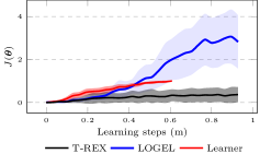
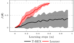
Refer to caption
Figure 9: The red line is the performance of the learner on the first 202020 steps of learning. The blue line is the performance of LOGEL on the first 303030 steps and the black line the performance of T-REX on the first 303030 steps of learning. The two algorithm are evaluated on the real reward weights. 101010 runs, 98% c.i.
Refer to caption
Figure 10: The red line is the performance of the learner on the first 202020 steps of learning. The black line the performance of T-REX on the first 303030 steps of learning. The algorithm is evaluated on the real reward weights.101010 runs, 98% c.i.
Refer to caption
Figure 11: The red line is the performance of the learner on the first 202020 steps of learning. The blue line is the performance of LOGEL on the first 303030 steps and the black line the performance of T-REX on the first 303030 steps of learning. The two algorithm are evaluated on the real reward weights.101010 runs, 98% c.i.

B.3 Autonomous driving scenario

In this section, we report an additional, preliminary experiment, that we perform on a simulator driving scenario. We employ SUMO simulator, an open-source, continuous road traffic simulation package designed to handle large road networks. SUMO focuses on the high-level control of the car, integrating an internal system that controls the vehicle dynamics. During the simulation, SUMO provides information on the other vehicles around the ego vehicle.

We consider a crossroad scenario which consists of an intersection with an arbitrary number of roads. The vehicle coming from the source road has to reach a target road that has a higher priority. The goal of the agent is to drive the ego car and enter the target road, avoiding dangerous maneuvers.

The reward features consists of four components:

  • Time: a constant feature at each decision step,

  • Jerk: the absolute value of the instantaneous jerk, i.e., the finite- difference derivative of the acceleration,

  • Harsh Slow Down: a binary feature, which activates whenever the velocity is lower than a threshold,

  • Crash: a binary feature which activates when the vehicle violates the safety constraints or performs a crash.

The agent’s policy is a rule-based policy, i.e., a set of parametrized rules, which is learned using Policy Gradients with Parameter-based Exploration (PGPE). It is important to notice that the agent’s policy is not differentiable.

We perform 101010 PGPE updates of the agents and then we use the learning trajectories with LOGEL. In the behavioral cloning step, we use a linear layer to approximate the policy of the learner. Table 1 shows the normalized weights recovered by LOGEL and the normalized real weights. As shown in Table 1 and in Figure 12, the reward weights recovered are quite similar to the real ones.

Time Jerk Slow Crash
Recovered Weights 0.0401 0.0174 0.0000 0.9424
Real Weights 0.0017 0.0003 0.0000 0.9980
Table 1: Reward weights for the autonomous simulate driving scenario.
Refer to caption
Figure 12: Reward weights for the autonomous simulate driving scenario.