III.2.2 Amplitude estimation based LCU evaluation
One inexpensive approach that can be used to estimate the expectation value comes from combining the Hadamard test circuit and amplitude estimation Brassard et al. (2002 ) .
Here we used a slightly generalized form of a generalized Hadamard test circuit shown in Figure III.2.2 . The expectation value of the first qubit for the above circuit is 1 / 2 + Re ( ⟨ ψ | C | ψ ⟩ ) / 2 .
In order to see this, consider the following,
| 0 ⟩ | 0 ⟩ | ψ ⟩ ↦ | 0 ⟩ ( ∑ ℓ w ℓ λ | ℓ ⟩ ) | ψ ⟩ ↦ + | 0 ⟩ | 1 ⟩ 2 ( ∑ ℓ w ℓ λ | ℓ ⟩ ) | ψ ⟩
↦ + | 0 ⟩ 2 ( ∑ ℓ w ℓ λ | ℓ ⟩ ) | ψ ⟩ | 1 ⟩ 2 ( ∑ ℓ w ℓ λ | ℓ ⟩ U ℓ | ψ ⟩ )
↦ + | 0 ⟩ 2 ( + ( prepare | 0 ⟩ ) | ψ ⟩ ∑ ℓ w ℓ λ | ℓ ⟩ U ℓ | ψ ⟩ ) | 1 ⟩ 2 ( - ( prepare | 0 ⟩ ) | ψ ⟩ ∑ ℓ w ℓ λ | ℓ ⟩ U ℓ | ψ ⟩ )
↦ + | 0 ⟩ 2 ( + | 0 ⟩ | ψ ⟩ prepare † ∑ ℓ w ℓ λ | ℓ ⟩ U ℓ | ψ ⟩ ) | 1 ⟩ 2 ( - | 0 ⟩ | ψ ⟩ | junk ⟩ ) . (122)
Therefore, the probability of measuring 0 in the top-most qubit in Figure III.2.2 is
= 1 4 ( + 2 ⟨ 0 | ⟨ ψ | prepare † ∑ ℓ w ℓ λ | ℓ ⟩ U ℓ | ψ ⟩ ( ⟨ 0 | ⟨ ψ | prepare † ∑ ℓ w ℓ λ | ℓ ⟩ U ℓ | ψ ⟩ ) ∗ ) + 1 Re ( ⟨ ψ | C | ψ ⟩ λ ) 2 . (123)
If amplitude estimation is used, the number of invocations of prepare and select needed to estimate this probability within ϵ error is 𝒪 ( λ / ϵ ) , which is a quadratic improvement over the sampling bound in Eq. (113 .
Following the same reasoning used to derive Eq. (119 we find that the over all Toffoli count is then, under the assumptions that the Toffoli count is dominated by applications of the prepare , select and phase circuit operations and further that the cost of adding an additional control to select is negligible, given by
4 π p J λ ( + C phase C Sel 2 C Prep ) Δ C . (124)
Here 𝒞 Sel and 𝒞 Prep are the Toffoli counts for select and prepare respectively.
Equation Eq. (124 shows that the favorable scalings of the sampling approach and the direct phase evaluation methods can be combined together in a single method. However, this advantage comes potentially at the price of a worse prefactor owing to the additional complexity of the prepare and select circuits. In particular, we find that this approach will be preferable to sampling and direct phase estimation, respectively, when
σ 2 ≥ 4 π λ Δ C ( + C phase C Sel 2 C Prep C phase ) , (125)
L ≥ + C phase C Sel 2 C Prep C Phase . (126)
In general, we suspect that in fault-tolerant settings this this approach will be preferable to direct phase oracle evaluation because the costs of the prepare and select circuits will often be comparable, or less than, that of 𝒰 ψ as we will see in the following section where we provide explicit constructions for the prepare and select oracles.
III.3 Adiabatic quantum optimization
III.3.1 Background on the adiabatic algorithm
The adiabatic algorithm Farhi et al. (2000b ) works by initializing a system as an easy-to-prepare ground state of a known Hamiltonian, and then slowly (adiabatically) deforming that system Hamiltonian into the Hamiltonian whose ground state we wish to prepare. For instance, we might use a Hamiltonian parameterized by ∈ s [ 0 , 1 ]
where H 0 H 1 = H ( 0 ) H 0 s = H ( 1 ) H 1 H 1
The main challenge with the adiabatic algorithm is that we may need to turn s s H ( s ) Δ T O ( / 1 Δ 2 ) | ψ k ( s ) ⟩ k th H ( s ) Elgart and Hagedorn (2012 )
∈ ‖ - T e - i ∫ 0 1 H ( x ) T d x | ψ k ( 0 ) ⟩ | ψ k ( 1 ) ⟩ ‖ ~ O ( 1 Δ 2 T ) , (128)
where Δ | ψ k ( s ) ⟩ ∈ T ( / 1 Δ 2 ϵ ) ϵ ~ O ( poly ( ‖ ˙ H ‖ , ‖ ¨ H ‖ , … ) ( + / 1 Δ 2 / log ( / 1 ϵ ) Δ ) ) ‖ ∂ s q H ( 0 ) ‖ = ‖ ∂ s q H ( 1 ) ‖ = 0 ∈ Q ( ϵ ) ( log ( / 1 ϵ ) ) ∈ ϵ ( Δ ) Lidar et al. (2009 ); Wiebe and Babcock (2012 ); Kieferová and Wiebe (2014 ) .
Note that the boundary adiabatic theorem only tells us about the state at the end of the evolution, and does not actually tell us anything the state we would be in at the middle of the evolution. For that there are “instantaneous” adiabatic theorems which bound the probability of being in the ground state throughout the entire evolution. For instance, one such way to show this is based on the Zeno stabilized adiabatic evolutions described in Section III.3.3 Boixo et al. (2009 ) .
These instantaneous adiabatic theorems have complexity ( / L 2 ( ϵ Δ ) )
is the path length.
In the case of simulated annealing, one can show that the path length is independent of Δ ≤ L / ‖ ˙ H ‖ Δ ( / ‖ ˙ H ‖ 2 Δ 3 ) Boixo et al. (2009 ) . It is not completely clear which style of adiabatic evolution will give the best results when using the approach as a heuristic, and so we discuss both here. With either approach we typically take H 1 H 0 = H 0 ∑ = i 1 N X i X i X | + ⟩ ⊗ N H 0
The simplest way to use the adiabatic algorithm as a heuristic is to discretize the evolution using product formulas. For instance, if we assume the adiabatic schedule in Eq. (127 then we could attempt to prepare the ground state as
∏ = k 1 M exp ( - i ( - M k M 2 ) H 0 T ) exp ( - i ( k M 2 ) H 1 T ) | ψ 0 ( 0 ) ⟩ , (130)
where M M T M T T
Of course, one can also easily extend this strategy to using higher-order product formulas, or to using either different adiabatic interpolations or adiabatic paths. For example, if we define
= U 2 ( - k 1 M , k M ) exp ( - i ( - M k / 1 2 2 M 2 ) H 0 T ) exp ( - i ( + k / 1 2 M 2 ) H 1 T ) exp ( - i ( - M k / 1 2 2 M 2 ) H 0 T ) , (131)
then we have that ∈ ‖ - ∏ = k 1 M U 2 ( - k 1 M , k M ) T exp ( - i ∫ 0 T H ( t ) d t ) ‖ O ( / T 3 M 2 ) ∈ s [ 0 , 1 ]
U ρ ( s , + s δ ) := U - ρ 2 ( + s [ - 1 γ ρ ] δ , + s δ ) U - ρ 2 ( + s [ - 1 2 γ ρ ] δ , + s [ - 1 γ ρ ] δ )
× U - ρ 2 ( + s 2 γ ρ δ , + s [ - 1 2 γ ρ ] δ ) U - ρ 2 ( + s γ ρ δ , + s 2 γ ρ δ ) U - ρ 2 ( s , + s γ ρ δ ) . (132)
Here = γ ρ ( - 4 4 / 1 ( - ρ 1 ) ) - 1 / 1 3 ρ
∈ ‖ - ∏ = k 1 M U ρ ( - k 1 M , k M ) T exp ( - i ∫ 0 T H ( t ) d t ) ‖ O ( / T + ρ 1 M ρ ) , (133)
which results in near linear scaling with T T
In practice, however, since the number of exponentials in the Trotter-Suzuki formula grows exponentially with the order there is in practice an optimal tradeoff in gate complexity that is satisfied by a finite order formula for a fixed ϵ T H 0 H 1 H 1 O phase Section II , the total cost of the procedure will be approximately M C phase M
= C adiabatic 2 M 5 - / ρ 2 1 C phase . (134)
Again, assuming that our target error in the adiabatic sweep is ϵ ∈ Δ 2 O ( ϵ ) ∈ T O ( / 1 Δ 2 ϵ ) M 2 - / ρ 2 1 ∈ M ( / T + 1 o ( 1 ) ϵ o ( 1 ) )
∈ C adiabatic C phase ( ϵ Δ 2 ) + 1 o ( 1 ) . (135)
Similarly, if we are interested in the limit where ∈ Δ 2 ω ( ϵ ) Lidar et al. (2009 ); Wiebe and Babcock (2012 ) can be used to improve the number of gates needed to reach the global optimum to
∈ C adiabatic C phase log + 1 o ( 1 ) ( / 1 ϵ ) Δ ( ϵ Δ ) o ( 1 ) . (136)
These results show that, provided the eigenvalue gap is polynomial, we can use a simulation routine for e - i H 1 ( t ) e - i H 0 ( t )
To give the cost for a single step a little more precisely, we can also include the cost of implementing a transverse driving field.
Since that involves applying a phase to b pha N + 1.15 N b pha ( N ) N + / b pha 2 2 O ( b pha log b pha ) + 4 N / b pha 2 2 O ( b pha log b pha ) + 3 log L ( 1 ) = b grad + b pha ( log b pha ) × 2 5 - / ρ 2 1 ρ
+ C phase 4 N / b pha 2 2 ( b pha log b pha ) (137)
for a single step.
III.3.2 Heuristic adiabatic optimization using quantum walks
While the procedure we described for heuristically using the adiabatic algorithm with Trotter based methods is well known, it is less clear how one might heuristically use LCU methods with the adiabatic algorithm. One reason we might try doing this is because the qubitized quantum walks that we discuss in Section II are sometimes cheaper to implement than Trotter steps for some problems. One approach to using LCU methods for adiabatic state preparation might be to directly attempt to simulate the time-dependent Hamiltonian evolution using a Dyson series approach, as was recently suggested for the purpose of adiabatic state preparation in Wan and Kim (2020 ) . However, this would require fairly complicated circuits due to the many time registers that one must keep to index the time-ordered exponential operator. In principle, we could always use quantum signal processing (or more generally quantum singular value transformations) to convert the walk operator at time t e - i H ( t ) δ δ
Instead, here we will suggest a strategy which is something of a combination between using qubitized quantum walks and using a product formula approximation. Our method is unlikely to be asymptotically optimal for this purpose but it is simple to implement and we suspect it would be cheaper than either a Dyson series approach or a Trotter approach for some applications on a small error-corrected quantum computer. The idea is to stroboscopically simulate time evolution as a short-time evolved “qubitized” walk. The result will be that we actually simulate the adiabatic path generated by the arccosine of the normalized Hamiltonian H ( s ) H ( s )
In the following we will assume that = select 2 1 | ψ k ( t ) ⟩ H ( t ) = H | ψ k ( t ) ⟩ E k ( t ) = | L ⟩ prepare | 0 ⟩
= W ( - I ⊗ 2 I | L ⟩ ⟨ L | ) select . (138)
The walk operator can be seen as a direct sum of two different walk operators, = W ⊕ W H W ⟂ W H = | ψ k ( t ) , L ⟩ ⊗ | ψ k ( t ) ⟩ | L ⟩ W ⟂ k t | ψ k ⟂ ( t ) ⟩
| ψ k ⟂ ( t ) ⟩ = ( - W E k ( t ) λ ( t ) ) | ψ k ( t ) , L ⟩ - 1 E k 2 ( t ) λ 2 ( t ) = ( - W H E k ( t ) λ ( t ) ) | ψ k ( t ) , L ⟩ - 1 E k 2 ( t ) λ 2 ( t ) , (139)
then we can express
= W H ( t ) exp ( - i ( - ∑ k i | ψ k ⟂ ( t ) ⟩ ⟨ ψ k ( t ) , L | i | ψ k ( t ) , L ⟩ ⟨ ψ k ⟂ ( t ) | ) arccos ( E k ( t ) λ ( t ) ) ) . (140)
It may be unclear how to implement a time-step for W ( t ) ≥ r 1
H ( t ) = ∑ k λ k ( t ) U k ↦ + ∑ k λ k ( t ) U k ( - r 1 ) λ ( t ) 2 ( - I I ) . (141)
In this case we can block encode the Hamiltonian using a unary encoding of the extra two operators via
= | L ( t , r ) ⟩ + ∑ k λ k ( t ) λ ( t ) r | k ⟩ | 00 ⟩ - r 1 2 r | 0 ⟩ ( + | 10 ⟩ | 11 ⟩ ) . (142)
The select oracles for this Hamiltonian require one additional control for each of the original terms in the Hamiltonian and the additional terms only need a single Pauli-Z select ′
With these two oracles defined, we can then describe the walk operator W r ( t ) t
= W r ( t ) ( - I ⊗ 2 I | L ( t , r ) ⟩ ⟨ L ( t , r ) | ) select ′ . (143)
This new Hamiltonian has exactly the same eigenvectors, however its value of λ r H ( t )
W H , r ( t ) = exp ( ( - i ( - ∑ k i | ψ k ⟂ ( t ) ⟩ ⟨ ψ k ( t ) , L ( t , r ) | i | ψ k ( t ) , L ( t , r ) ⟩ ⟨ ψ k ⟂ ( t ) | ) r arccos ( E k ( t ) r λ ( t ) ) ) 1 r ) . (144)
Using the fact that = arccos ( x ) - / π 2 arcsin ( x )
= V H , r ( t ) exp ( ( i ( - ∑ k i | ψ k ⟂ ( t ) ⟩ ⟨ ψ k ( t ) , L ( t , r ) | i | ψ k ( t ) , L ( t , r ) ⟩ ⟨ ψ k ⟂ ( t ) | ) r arcsin ( E k ( t ) r λ ( t ) ) ) 1 r ) . (145)
Thus the operator V H , r ( t ) / 1 r
:= H r ( t ) ( - ∑ k i | ψ k ⟂ ( t ) ⟩ ⟨ ψ k ( t ) , L ( t , r ) | i | ψ k ( t ) , L ( t , r ) ⟩ ⟨ ψ k ⟂ ( t ) | ) r arcsin ( E k ( t ) r λ ( t ) ) . (146)
Note that as → r ∞ ± / E k ( t ) λ ( t )
sin ^-1(E_k(t)/(r λ (t))) - E_k(t)/ λ (t)— ∈O(1/r^2).
For any fixed value of r we can choose an adiabatic path between an initial Hamiltonian and a final Hamiltonian. The accuracy of the adiabatic approximation depends strongly on how quickly we traverse this path so it is customary to introduce a dimensionless time s = t / T which allows us to easily change the speed without altering the shape of the adiabatic path. In Appendix B we are able to show that the adiabatic theorem then implies that the number of steps of the quantum walk required to achieve error ϵ in an adiabatic state preparation for a maximum rank Hamiltonian with gap Δ is in
~ O ( 1 ϵ / 3 2 + max s ( + ‖ ¨ H ‖ | ¨ λ | ) max s ( + | ˙ λ | ‖ ˙ H ‖ ) min ( Δ , min k | E k | ) 2 λ max s ( | ˙ λ | + ∥ ˙ H ∥ ) 3 min ( Δ , min k | E k | ) 4 ) . (147)
The reason why this result depends on the minimum value of E k is an artifact of the fact that several of the eigenvalues of the walk operator can be mapped to 1 under repeated application of W r . This potentially can alter the eigenvalue gaps for eigenvalues near zero which impacts the result.
The key point behind this scaling is that it shows that as the number of time slices increases this heuristic converges to the true adiabatic path. Just as the intuition behind Trotterized adiabatic state preparation hinged on this fact, here this result shows that we can similarly use a programmable sequence of parameterizable walk operators to implement the dynamics. The main advantage relative to Trotter methods is that the price that we have to pay using this technique does not depend strongly on the number of terms in the Hamiltonian which can lead to advantages in cases where the problem or driver Hamiltonians are complex.
This scaling can be improved by using higher-order splitting formulas for the time evolution Wiebe et al. (2010 ) and by using boundary cancellation methods to improve the scaling of the error in adiabatic state preparation. In general, if we assume that Δ ∈ O ( 1 ) for the problem at hand then it is straightforward to see that we can improve the scaling from O ( 1 / ϵ 3 / 2 ) to 1 / ϵ o ( 1 ) Lidar et al. (2009 ); Wiebe and Babcock (2012 ); Kieferová and Wiebe (2014 ) . It is also worth noting that the bounds given above for the scaling with respect to the derivatives of the Hamiltonian and the coefficients of the Hamiltonian is expected to be quite loose owing to the many simplifying bounds used to make the expression easy to use. On the other hand, the scaling with the gap and error tolerance is likely tighter.
III.3.3 Zeno projection of adiabatic path via phase randomization
The principle of the Zeno approach is to increment the parameter for the Hamiltonian s β Lemieux et al. (2020a , b ) , and combined with a rewind procedure to give a significant reduction in gate complexity compared to other approaches.
An alternative approach was proposed in Boixo et al. (2009 ); Chiang et al. (2014 ) , where the measurement was replaced with phase randomization.
Here we summarize this method and show how to further optimize it.
When using phase estimation, if it verifies that the system is still in the ground state, one continues with incrementing the parameter.
If the ground state is not obtained from the phase estimation, one could abort, in which case no output is given and one needs to restart.
Because the probability of failure is low, one could just continue regardless, and check at the end.
That means that the result of the phase estimation is discarded.
The phase estimation is performed with control qubits controlling the time of the evolution, then an inverse quantum Fourier transform on the control qubits to give the phase.
But, if the result of the measurement is ignored, then one can simply ignore the inverse quantum Fourier transform, and regard the control qubits as being measured in the computational basis and the result discarded.
That is equivalent to randomly selecting values for these control qubits in the computational basis at the beginning.
But, if these qubits take random values in the computational basis, one can instead just classically randomly generate a time, and perform the evolution for that time.
In performing a phase measurement using control qubits, one uses a superposition state on those control qubits, and the error in the phase measurement corresponds to the Fourier transform of those amplitudes.
That is, with b
= | χ ϕ ⟩ ∑ = z 0 - 2 b 1 e i z ϕ χ z | z ⟩ , (148)
where ϕ - E δ t | ^ ϕ ⟩ ⟨ ^ ϕ |
= | ^ ϕ ⟩ 1 2 π ∑ = z 0 - 2 b 1 e i z ^ ϕ | z ⟩ . (149)
The probability distribution for the error = δ ϕ - ^ ϕ ϕ
Pr ( δ ϕ ) = | ⟨ ^ ϕ | χ ϕ ⟩ | 2 = 1 2 π | ∑ = z 0 - 2 b 1 e i z δ ϕ χ z | . (150)
These measurements are equivalent to the theory of window functions in spectral analysis. A particularly useful window to choose is the Kaiser window, because it has exponential suppression of errors Kaiser and Schafer (1980 ) .
In the case where the evolution time is chosen classically, it can be given by a real number, and we do not need any bound on the evolution time.
Then the the expected cost is the expectation value of | t |
= ⟨ | t | ⟩ ∫ d t | t | p time ( t ) . (151)
Because there is no upper bound on t
= | ψ E ⟩ ∫ d t e - i E t χ t | t ⟩ , (152)
where E t = p time ( t ) | χ t | 2 | ^ E ⟩ ⟨ ^ E |
= | ^ E ⟩ 1 2 π ∫ d t e - i ^ E t | t ⟩ . (153)
The probability distribution for the error in the measurement of E
= Pr ( δ E ) 1 2 π | ∫ d t e i t δ E χ t | 2 . (154)
An alternative description is to describe the system as being in state
where | ψ j ⟩ E j t p time ( t )
∑ j , k ⟨ ψ j | ψ ⟩ ⟨ ψ | ψ k ⟩ ~ p time ( - E j E k ) | ψ j ⟩ ⟨ ψ k | , (156)
where
= ~ p time ( - E j E k ) ∫ d t p time ( t ) e - i ( - E j E k ) t . (157)
If the width of the Fourier transform of the probability distribution p time Δ
∑ j | ⟨ ψ j | ψ ⟩ | 2 | ψ j ⟩ ⟨ ψ j | . (158)
In comparison, if Pr ( δ E ) ≤ | δ E | E max = 2 E max Δ = p time ( t ) χ t 2 p time χ t
Next we consider appropriate probability distributions.
A probability distribution for t Boixo et al. (2009 ) was
= p time ( t ) 8 π sinc 4 ( / t Δ 4 ) 3 Δ . (159)
That gives = ⟨ | t | ⟩ / 12 ln 2 ( π Δ ) ≈ ⟨ | t | ⟩ Δ 2.648 Pr ( δ E )
= Pr ( δ E ) 2 Δ ( - 1 | / 2 δ E Δ | ) . (160)
Then the corresponding ψ t Pr ( δ E )
= χ t - sin ( / Δ t 2 ) C ( / Δ t π ) cos ( / Δ t 2 ) S ( / Δ t π ) ( / Δ t 2 ) / 3 2 , (161)
where C S = ⟨ | t | ⟩ / 7 ( 3 Δ ) ≈ ⟨ | t | ⟩ Δ 2.333
To find the optimal window, we can take
= 1 2 π ∫ d t e i t x χ t ( - 1 x 2 ) ∑ ℓ a ℓ x 2 ℓ , (162)
for x E max ( - 1 x 2 ) ± 1
= χ t 1 2 π ∑ ℓ a ℓ ∫ - 1 1 d x cos ( x t ) ( - 1 x 2 ) x 2 ℓ . (163)
Then the expectation of the absolute value of the time is
= ∫ d t | t | | χ t | 1 2 π ∑ k , ℓ a k a ℓ A k ℓ , (164)
where
= A k ℓ ∫ d t | t | ( ∫ - 1 1 d x cos ( x t ) ( - 1 x 2 ) x 2 k ) ( ∫ - 1 1 d z cos ( z t ) ( - 1 z 2 ) z 2 ℓ ) . (165)
We also need, for normalization,
1 = ∑ k , ℓ a k a ℓ ∫ - 1 1 d x ( - 1 x 2 ) 2 x 2 ( + k ℓ ) = ∑ k , ℓ a k a ℓ B k ℓ , (166)
where
= B k ℓ 16 [ + 2 ( + k ℓ ) 1 ] [ + 2 ( + k ℓ ) 3 ] [ + 2 ( + k ℓ ) 5 ] . (167)
Then defining = → b B / 1 2 → a = ‖ → b ‖ 1 ⟨ | t | ⟩ / → a T A → a π / → a T B - / 1 2 A B - / 1 2 → a π B - / 1 2 A B - / 1 2 ≈ ⟨ | t | ⟩ E max 1.1580 a 22
This explanation is for the case where there is Hamiltonian evolution for a time t e ± i arccos ( / H λ ) t / 1 λ λ
III.4 Szegedy walk based quantum simulated annealing
In the remainder of Section III we consider quantum simulated annealing, where the goal is to prepare a coherent equivalent of a Gibbs state and cool to a low temperature.
More specifically, the coherent Gibbs state is
:= | ψ β ⟩ ∑ ∈ x Σ π β ( x ) | x ⟩ , ∝ π β ( x ) exp ( - β E x ) , (168)
where β y x Pr ( | y x )
= Pr ( | y x ) π β ( x ) Pr ( | x y ) π β ( y ) . (169)
The detailed balance condition ensures that π β y x
:= Pr ( | y x ) / min { 1 , exp ( β ( - E x E y ) ) } N , (170)
and = Pr ( | x x ) - 1 ∑ ≠ y x Pr ( | y x ) Lemieux et al. (2020a ) .
Another choice, used in Boixo et al. (2015 ) , is
= Pr ( | y x ) χ exp ( β ( - E x E y ) ) χ
= ⟨ x | H β | y ⟩ - δ x , y Pr ( | x y ) Pr ( | y x ) , (171)
then the detailed balance condition ensures that the ground state is | ψ β ⟩ β
In the approach of Somma et al. (2008 ) , the method used is to instead construct a quantum walk where the quantum Gibbs state is an eigenstate.
One could change the value of β β | ψ β ⟩ Somma et al. (2008 ) also proposes using a random number of steps of the walk operator to achieve the same effect as the measurement.
The advantage of using the quantum walk is that the complexity scales as O ( / 1 δ ) δ H β ( / 1 δ )
The quantum walk used in Somma et al. (2008 ) is based on a Szegedy walk, which involves a controlled state preparation, a swap between the system and the ancilla, and inversion of the controlled state preparation.
Then a reflection on the ancilla is required.
The sequence of operations is as shown in Figure 9 .
The dimension of the ancilla needed is the same as the dimension as the system.
The reflection and swap have low cost, so the Toffoli cost is dominated by the cost of the controlled state preparation.
The Szegedy approach builds a quantum walk in a similar way as the LCU approach in Figure 2 , where there is a block encoded operation followed by a reflection Low and Chuang (2019 ) .
That is, preparation of the ancilla in the state | 0 ⟩ U | 0 ⟩ = A ⟨ 0 | U | 0 ⟩ | 0 ⟩ A e ± i arccos a a A
Here the controlled state preparation is of the form
cprep | x ⟩ | 0 ⟩ = ∑ y Pr ( | y x ) | x ⟩ | y ⟩ ≡ | α x ⟩ , (172)
where the sum is taken over all y x
= ⟨ 0 | cprep † swap cprep | 0 ⟩ ∑ x , y Pr ( | x y ) Pr ( | y x ) | y ⟩ ⟨ x | . (173)
Thus the block-encoded operation has a matrix representation of the form Pr ( | x y ) Pr ( | y x ) - 1 H β | ψ β ⟩ Berry et al. (2018 ); Poulin et al. (2018 ) . It is this arccosine that causes a square root improvement in the scaling with the spectral gap.
This is because if the block-encoded operation has gap δ E 2 δ E
In implementing the step of the walk, the state preparation requires calculation of each of the Pr ( | y x ) x Pr ( | x x ) ≡ Pr ( | x x ) - 1 ∑ ≠ y x Pr ( | y x )
= | ψ x ⟩ ∑ k Pr ( | x k x ) | x ⟩ | k ⟩ , (174)
where x k k x = k 0 | k ⟩ | α x ⟩ cnot s between the respective bits of the two registers.
In order to prepare the state | ψ x ⟩ > k 0
1.
Compute N Pr ( | x k x ) N N N Pr ( | x x ) ≤ N Pr ( | x k x ) 1 b sm N Pr ( | x x ) + ⌈ log N ⌉ b sm b sm N ( + ⌈ log N ⌉ b sm )
2.
We have N
| 0 ⟩ A | 0 ⟩ K | 0 ⟩ Z | 0 ⟩ ZZ | 0 ⟩ B | 0 ⟩ C , (175)
where K is the target system, A , B , and C are single-qubit ancillas, and Z and ZZ are s ZZ and B .
| + ⟩ A | 0 ⟩ K 1 2 / s 2 ∑ = z 0 - 2 s 1 | z ⟩ Z | 0 ⟩ ZZ | 0 ⟩ B | + ⟩ C . (176)
3.
Controlled on ancilla A ⌈ log N ⌉ K .
If N log N T N ( log N ) Section III.5.2 .
4.
We can map the binary to unary in place, with cost no more than - N log N Appendix C ), to give
1 2 / s 2 2 ( + | 0 ⟩ A | 0 ⟩ K 1 N | 1 ⟩ A ∑ = k 1 N | k ⟩ K ) ∑ = z 0 - 2 s 1 | z ⟩ Z | 0 ⟩ ZZ | 0 ⟩ B | + ⟩ C , (177)
where | k ⟩ K
5.
Compute the approximate square of z ~ z 2 ZZ , to give
1 2 / s 2 2 ( + | 0 ⟩ A | 0 ⟩ K 1 N | 1 ⟩ A ∑ = k 1 N | k ⟩ K ) ∑ = z 0 - 2 s 1 | z ⟩ Z | ~ z 2 ⟩ ZZ | 0 ⟩ B | + ⟩ C . (178)
The complexity is no greater than / s 2 2 Appendix D.6 .
To obtain b sm = s + b sm ( log b sm ) + / b sm 2 2 ( b sm log b sm )
6.
For each = k 1 , … , N N Pr ( | x k x ) z 2 ZZ register, controlled by qubit k K , placing the result in B .
This has cost N b sm
7.
Controlled on ancilla A being zero, perform an inequality test between N Pr ( | x x ) N z 2 B .
The inequality test has complexity b sm N N + b sm 2 ( b sm log b sm ) b sm N N
1 2 / s 2 2 ( | 0 ⟩ A | 0 ⟩ K ∑ = z 0 - 2 s ~ Pr ( | x x ) 1 | z ⟩ Z | ~ z 2 ⟩ ZZ | 0 ⟩ B + | 0 ⟩ A | 0 ⟩ K ∑ = z 2 s ~ Pr ( | x x ) - 2 s 1 | z ⟩ Z | z 2 ⟩ ZZ | 1 ⟩ B (179)
+ 1 N | 1 ⟩ A ∑ = k 1 N | k ⟩ K ∑ = z 0 - 2 s N ~ Pr ( | x k x ) 1 | z ⟩ Z | ~ z 2 ⟩ ZZ | 0 ⟩ B + 1 N | 1 ⟩ A ∑ = k 1 N | k ⟩ K ∑ = z 2 s N ~ Pr ( | x k x ) - 2 s 1 | z ⟩ Z | ~ z 2 ⟩ ZZ | 1 ⟩ B ) | + ⟩ C , (180)
where ~ Pr z
8.
Uncompute z 2 ZZ with complexity no more than / s 2 2
9.
Use a sequence of CNOTs with the N K as controls and ancilla A as target.
This will reset A to zero.
10.
Perform Hadamards on the qubits of K , giving a state of the form
+ 1 2 | 0 ⟩ A ( + ~ Pr ( | x x ) | 0 ⟩ K 1 N ∑ = k 1 N ~ Pr ( | x k x ) | k ⟩ K ) | 0 ⟩ Z | 0 ⟩ ZZ | 0 ⟩ B | 0 ⟩ C | ψ ⟂ ⟩ , (181)
where | ψ ⟂ ⟩ Z B C
11.
Now conditioned on | 0 ⟩ Z | 0 ⟩ B | 0 ⟩ C / 1 2 | 0 ⟩ Z | 0 ⟩ B | 0 ⟩ C s + N ( b sm )
The overall Toffoli complexity of this procedure, excluding the computation of Pr ( | x k x )
+ N ( + ⌈ log N ⌉ b sm ) N 3 [ + N b sm 2 2 b sm 2 ( + N 1 ) b sm ] ( + log N b sm log b sm ) . (182)
Here is first term is for the subtractions in step 1, the second term N N b sm 2 z 2 2 b sm 2 N N ( + N 1 ) b sm + N 1 log N b sm log b sm
Note that the preparation will not be performed perfectly, because the initial amplitude is not exactly / 1 2 swap .
To see the effect of this procedure, suppose the system is in basis state x
= cprep | 0 ⟩ | x ⟩ | 0 ⟩ + μ x | 1 ⟩ | x ⟩ ∑ y Pr ( | y x ) | y ⟩ ν x | 0 ⟩ | x ⟩ | ϕ x ⟩ (183)
where the first qubit flags success, μ y ν x ϕ x x Pr ( | y x ) swap is only performed in the case of success, which gives
= swap cprep | 0 ⟩ | x ⟩ | 0 ⟩ + μ x | 1 ⟩ ∑ y Pr ( | y x ) | y ⟩ | x ⟩ ν x | 0 ⟩ | x ⟩ | ϕ x ⟩ . (184)
Then we can write
= ⟨ 0 | ⟨ y | ⟨ 0 | cprep † + μ y | 1 ⟩ ∑ x Pr ( | x y ) ⟨ y | ⟨ x | ν y ⟨ 0 | ⟨ y | ⟨ ϕ y | , (185)
so
⟨ 0 | ⟨ y | ⟨ 0 | cprep † swap cprep | 0 ⟩ | x ⟩ | 0 ⟩ = + μ x μ y Pr ( | y x ) Pr ( | x y ) δ x , y ν x 2
= Pr ′ ( | y x ) Pr ′ ( | x y ) , (186)
where we define
= Pr ′ ( | x y ) { μ y 2 Pr ( | x y ) , ≠ x y - 1 μ y 2 ∑ ≠ z y Pr ( | z y ) , = x y . (187)
That is, the effect of the imperfect preparation is that the qubitized step corresponds to a slightly lower probability of transitions, which should have only a minor effect on the optimization.
The cost of the quantum walk in this approach is primarily in computing all transition probabilities N Pr ( | x k x ) > k 0 N Pr ( | x x ) N Pr ( | x k x ) N Pr ( | x k x )
1.
Query the energy difference oracle to find the energy difference
δ E b dif
2.
Calculate exp ( - β δ E ) b sm Section II.5 .
The costs for the energy difference oracles were discussed in Section II.1 , and are as in Table 4 .
In this table, the costs for the energy difference oracles for the L N N x x k + N 1 N N N N + N 1 N
Figure 8:
The qubitized quantum walk operator W Figure 9:
The quantum walk operator using the Szegedy approach, where we have moved the controlled preparation to the end.
To perform the state preparation, we need to compute the energy differences, use those to compute the transition probabilities, prepare the state, then uncompute the transition probabilities and energy differences.
In each step of the Szegedy walk as shown in Figure 9 , we need to do the controlled preparation and inverse preparation, which means that the energy differences and need to be computed four times for each step.
That would give a cost of
+ min ( 4 ( + N 1 ) C direct , 4 N C diff ) 4 N C fun . (188)
However, we can save a factor of two by taking the controlled preparation and moving it to the end of the step, as shown in Figure 9 .
The reason why we can save a factor of two is that then, in between the controlled inverse preparation and preparation, there is a reflection on the target, but the control is not changed.
That means we can keep the values of the energy differences and transition probabilities computed in the controlled inverse preparation without uncomputing them, then only uncompute them after the controlled preparation.
This approach does not change the effect of a sequence of steps if β β Figure 9 will be different to that taking the controlled preparation and moving it to the end of the state.
That is, the value of β
+ min ( 2 ( + N 1 ) C direct , 2 N C diff ) 2 N C fun . (189)
Now adding twice the complexity of the state preparation from Eq. (182 gives complexity
+ min ( 2 ( + N 1 ) C direct , 2 N C diff ) 2 N C fun 2 N log N 8 N b sm 18 b sm 2 ( N ) . (190)
Here we have omitted b sm log b sm N 9 b sm 2 3 b sm 2 6 b sm 2 N 6 b sm 2
To evaluate the numbers of ancillas needed, we need to distinguish between the persistent ancillas and temporary ancillas in Table 4 .
This is because the persistent ancillas need to be multiplied by N
1.
The N
2.
N
3.
N
4.
The ancillas Z , A , B , C in the state preparation use + b sm ( log b sm )
For the temporary ancillas, we have contributions from the energy difference evaluation, the function evaluation, and the state preparation.
Since these operations are not done concurrently, we can take the maximum of the costs.
The most significant will be that for the state preparation.
In the state preparation we have costs
1.
Ancilla ZZ has + b sm ( log b sm )
2.
If N + b sm ( log b sm ) N z 2
3.
We use + b sm ( log b sm ) + 2 b sm ( log b sm ) N
As a result, the temporary ancilla cost is + 2 b sm ( log b sm ) N + 4 b sm ( log b sm ) N
+ N A diff N A fun 5 b sm ( log b sm ) . (191)
III.5 LHPST qubitized walk based quantum simulated annealing
The same quantum walk approach to quantum simulated annealing can be achieved using an improved form of quantum walk given by Lemieux, Heim, Poulin, Svore, and Troyer (LHPST) Lemieux et al. (2020a ) that requires only computation of a single transition probability for each step.
Here we provide an improved implementation of that quantum walk that can be efficiently achieved for more general types of cost Hamiltonians than considered in Lemieux et al. (2020a ) .
The operations used to achieve the step of the walk are
where
: V → | 0 ⟩ M 1 N ∑ j | j ⟩ M , (193)
: B → | x ⟩ S | j ⟩ M | 0 ⟩ C | x ⟩ S | j ⟩ M ( + - 1 p x , x j | 0 ⟩ C p x , x j | 1 ⟩ C ) , (194)
: F → | x ⟩ S | j ⟩ M | 0 ⟩ C | x ⟩ S | j ⟩ M | 0 ⟩ C , → | x ⟩ S | j ⟩ M | 1 ⟩ C | x j ⟩ S | j ⟩ M | 1 ⟩ C , (197)
: R → | 0 ⟩ M | 0 ⟩ C - | 0 ⟩ M | 0 ⟩ C , | j ⟩ M | c ⟩ C → | j ⟩ M | c ⟩ C for ( j , c ) ≠ ( 0 , 0 ) . (200)
Here = p x , y N Pr ( | y x ) j
This walk is equivalent to the Szegedy approach of Somma et al. (2008 ) because it yields the same block-encoded operation. That is,
⟨ 0 | V † B † F B V | 0 ⟩ Pr ( | x y ) Pr ( | y x )
V | 0 ⟩ M | 0 ⟩ C = 1 N ∑ = j 1 N | j ⟩ M | 0 ⟩ C , (201)
B V | 0 ⟩ M | 0 ⟩ C = 1 N ∑ x ∑ = j 1 N ⊗ | x ⟩ ⟨ x | | j ⟩ ( + - 1 p x , x j | 0 ⟩ C p x , x j | 1 ⟩ C ) , (202)
F B V | 0 ⟩ M | 0 ⟩ C = + 1 N ∑ x ∑ = j 1 N ⊗ | x ⟩ ⟨ x | | j ⟩ - 1 p x , x j | 0 ⟩ C 1 N ∑ x ∑ = j 1 N ⊗ | x j ⟩ ⟨ x | | j ⟩ p x , x j | 1 ⟩ C
= + 1 N ∑ x ∑ = j 1 N ⊗ | x ⟩ ⟨ x | | j ⟩ - 1 p x , x j | 0 ⟩ C 1 N ∑ x ∑ = j 1 N ⊗ | x ⟩ ⟨ x j | | j ⟩ p x j , x | 1 ⟩ C , (203)
⟨ 0 | C M ⟨ 0 | V † B † F B V | 0 ⟩ M | 0 ⟩ C = + 1 N ∑ x ∑ = j 1 N | x ⟩ ⟨ x | ( - 1 p x , x j ) 1 N ∑ x ∑ = j 1 N | x ⟩ ⟨ x j | p x , x j p x j , x
= + ∑ x | x ⟩ ⟨ x | ( - 1 1 N ∑ = j 1 N p x , x j ) 1 N ∑ x ∑ = j 1 N | x j ⟩ ⟨ x | p x , x j p x j , x
= ∑ x , y | y ⟩ ⟨ x | Pr ( | y x ) Pr ( | x y ) . (204)
Just as with the Szegedy approach, most operations are trivial to perform, and the key difficulty is in the operation B B one transition probability, whereas the Szegedy approach requires computing all the transition probabilities for a state preparation.
Lemieux et al. Lemieux et al. (2020a ) propose a method for the B
That is, one considers the qubits that the transition probability for the move (here a bit flip) depends on, and classically precomputes the rotation angle for each basis state on those qubits.
For each value of j C Lemieux et al. (2020a ) is O ( 2 | N j | | N j | log ( / 1 ϵ ) ) | N j | j | N j | O ( log ( / 1 ϵ ) ) j N j O ( N 2 | N j | [ + | N j | log ( / 1 ϵ ) ] )
To improve the complexity, one can divide this procedure into two parts, where first a QROM is used to output the desired rotation in an ancilla, and then those qubits are used to control a rotation.
Using the QROM procedure of Babbush et al. (2018 ) to output the required rotation, the cost in terms of Toffoli gates is O ( N 2 | N j | ) Section II.3 .
Addition of the register containing the rotation to an ancilla with state | ϕ ⟩ (34 results in a phase rotation.
To rotate the qubit, simply make the addition controlled by this qubit, and use Clifford gates before and after so that the rotation is in the y O ( log ( / 1 ϵ ) ) Appendix A .
With that improvement the complexity is reduced to O ( + N 2 | N j | log ( / 1 ϵ ) )
Even with that improvement, any procedure of that type is exponential in the number of qubits that the energy difference depends on, | N j | Lemieux et al. (2020a ) , but here we consider Hamiltonians typical of real world problems where the energy difference will depend on most of the system qubits, because the Hamiltonians have high connectivity.
We thus propose alternative procedures to achieve the rotation B
III.5.1 Rotation B
We propose a completely different method to perform the rotation B Lemieux et al. (2020a ) .
We can first compute the energy difference - E x E x j arcsin p x , x j C arcsin p x , x j arcsin p x , x j Häner et al. (2018 ) .
For the purposes of quantum optimization, we expect that we will not need to compute this function to high precision as long as the function we compute is still monotonic in the actual energy, so there is the opportunity to use methods that are very efficient for low precision but would not be suitable for high precision.
We propose a method based on using a piecewise linear approximation, with the coefficients output by a QROM, as described in Section II.5 .
One could then apply the controlled rotation with cost b sm (34 , as described in detail in Appendix A .
Then after uncomputing the rotation angle we would have implemented B arcsin p x , x j B B
It is possible to halve that cost by only computing and uncomputing once in a step, and retaining the value of arcsin p x , x j F F j x x x j - E x E x j
1.
Compute the energy difference between x x j - E x E x j
2.
Compute arcsin p x , x j | - E x E x j |
3.
If < E x j E x X C cnot (Clifford) controlled by the sign bit of - E x E x j
4.
The remaining rotations for the case of > E x j E x
5.
When we apply F x x j - E x E x j C cnot , with no non-Clifford cost.
6.
Then at the end we uncompute arcsin p x , x j - E x E x j
This procedure assumes that - E x E x j - E x E x j b dif + 2 C diff 2 C fun 2 b dif O ( 1 )
III.5.2 Equal superposition V
The operation V
In the case where N not a power of 2, we can rotate an ancilla qubit such that the net amplitude is / 1 2 | 1 ⟩ | 1 ⟩ + 4 log N ( 1 )
Our method for V Lemieux et al. (2020a ) .
There they proposed encoding the M N N
Our procedure to create an equal superposition over < N 2 k
Then we have an inequality test between j N
+ 1 2 k ∑ = j 0 - 2 k 1 | j ⟩ | 1 ⟩ 1 2 k ∑ = j N - 2 k 1 | j ⟩ | 0 ⟩ . (207)
This is an inequality test on k constant we save a Toffoli gate. The cost is therefore - k 2 Berry et al. (2019 ) .
We would have an amplitude of / N 2 k 1 2 / 2 k N / 1 2 1 2 / 2 k N Appendix A to give
We can then perform a single step of amplitude amplification for | 1 ⟩
The steps needed in the amplitude amplification and their costs are as follows.
If we use the procedure for the rotation with s - s 3
1.
A first inequality test (- k 2 - s 3
2.
A first reflection on the rotated qubit and the result of the inequality test. This just needs a controlled phase (a Clifford gate).
3.
Inverting the rotation and inequality test has cost - + k s 5
4.
Hadamards then reflection of the k - k 1
5.
Applying the inequality test (- k 2
The total cost is - + 4 k 2 s 13
Conditioned on success of the inequality test, the state is
1 2 k ∑ = j 0 - N 1 | j ⟩ [ + ( - 1 4 N sin 2 θ 2 k ) | 0 ⟩ 2 sin θ ( + sin θ | 0 ⟩ cos θ | 1 ⟩ ) ] | 1 ⟩ . (209)
The probability for success is then given by the normalization
N 2 k [ + ( + - 1 4 N sin 2 θ 2 k 2 sin 2 θ ) 2 4 sin 2 θ cos 2 θ ] . (210)
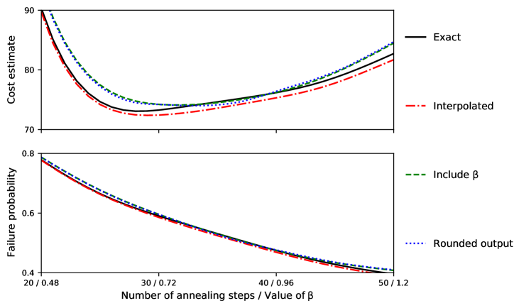
It is found that highly accurate results are obtained for = s 7 10
Figure 10: The probability for success using a rotation of the form / 2 π 2 s = s 7
This procedure enables construction of equal superposition states flagged by an ancilla qubit for N = s 7 + 4 k 1
III.5.3 Controlled bit flip F
We also need to modify the operation F M j x C | 1 ⟩
: F → | x ⟩ S | j ⟩ M | 0 ⟩ C | x ⟩ S | j ⟩ M | 0 ⟩ C , → | x ⟩ S | j ⟩ M | 1 ⟩ C | x j ⟩ S | j ⟩ M | 1 ⟩ C . (211)
This operation can be achieved using the iteration procedure of Babbush et al. (2018 ) with Toffoli complexity N M
A complication is that, in the case where N V F C | 1 ⟩
To be more specific, V
= V | 0 ⟩ + | 1 ⟩ | ψ 1 ⟩ | 0 ⟩ | ψ 0 ⟩ , (212)
with the first register flagging success.
Since we only perform F | 1 ⟩
= B † F B V | 0 ⟩ + B † F B | 1 ⟩ | ψ 1 ⟩ 1 | 0 ⟩ | ψ 0 ⟩ . (213)
To determine the block encoded operation
we note that
= ⟨ 0 | V † + ⟨ 1 | ⟨ ψ 1 | ⟨ 0 | ⟨ ψ 0 | , (215)
so
= ⟨ 0 | V † B † F B V | 0 ⟩ + ⟨ ψ 1 | B † F B | ψ 1 ⟩ 1 ⟨ ψ 0 | ψ 0 ⟩ , (216)
where 1
III.5.4 Reflection R
This operation applies a phase flip for zero on the ancillas as
: R → | 0 ⟩ M | 0 ⟩ C - | 0 ⟩ M | 0 ⟩ C ,
| j ⟩ M | c ⟩ C → | j ⟩ M | c ⟩ C for ( j , c ) ≠ ( 0 , 0 ) . (217)
As well as the ancillas M C ⌈ log N ⌉ j C + ⌈ log N ⌉ 2 ⌈ log N ⌉
III.5.5 Total costs
The total Toffoli costs of implementing = ~ U W R V † B † F B V
1.
The cost of V V † + 8 log N ( 1 )
2.
The cost of F N
3.
4.
The cost of two applications of B + 2 C diff 2 C fun 2 b dif O ( 1 )
The total cost of a step is then
+ 2 C diff 2 C fun N 2 b dif 9 log N ( 1 ) . (218)
Note that 8 log N N
1.
The ancilla registers M C + ⌈ log N ⌉ 1
2.
The resource state used to implement the controlled rotations needs b sm
3.
The ancilla requirements of the energy difference and function evaluation oracles.
For the temporary ancilla cost, we need to take the maximum of that for the energy difference and function evaluation, giving the total ancilla cost of
+ A diff A fun max ( B diff , B fun ) log N b sm ( 1 ) . (219)
III.6 Spectral gap amplification based quantum simulated annealing
An alternative, and potentially simpler, approach to preparing a low-temperature thermal state is given by Boixo et al. (2015 ) . The idea behind this approach is to construct a Hamiltonian whose ground state is a purification of the Gibbs state.
Similarly to the case with the quantum walk, one can start with an equal superposition state corresponding to infinite temperature, and simulate the Hamiltonian evolution starting from = β 0 β
A simple choice of Hamiltonian is similar to the block-encoded operation for the quantum walks, so has a small spectral gap.
In order to obtain a speedup, one needs to construct a new Hamiltonian with the square root of the spectral gap of the original Hamiltonian, thus yielding the same speedup as the quantum walks.
That procedure, from Boixo et al. (2015 ) , is called spectral gap amplification.
Simulating the time-dependent Hamiltonian, for example using a Dyson series, has significant complexity.
To avoid that complexity, here we suggest that one instead construct a step of a quantum walk using a linear combination of unitaries.
Such a quantum walk could be used to simulate the Hamiltonian evolution, but as discussed in Berry et al. (2018 ); Poulin et al. (2018 ) one can instead just perform steps of the quantum walk which has eigenvalues that are the exponential of the arccosine of those for the Hamiltonian.
By applying the steps of the quantum walk we can obtain the advantage of the spectral gap amplification, without the difficulty of needing to simulate a time-dependent Hamiltonian.
Unlike the quantum walks in the previous subsections, the arccosine does not yield a further square-root amplification of the spectral gap, because the relevant eigenvalue for the amplified Hamiltonian is not at 1. However, it potentially gives other scaling advantages (for instance, in avoiding the need for quantum signal processing when using certain oracles) compared to other proposals in the literature for realizing quantum simulated annealing via spectral gap amplification.
III.6.1 The spectral gap amplification Hamiltonian
Here we summarise the method of spectral gap amplification from Boixo et al. (2015 ) , but specialise to the case where only single bit flips are allowed to make the method clearer.
As discussed above, one can use a Hamiltonian simulation approach with Hamiltonian H β (171 with ground state corresponding to the quantum Gibbs state | ψ β ⟩ Boixo et al. (2015 ) is to construct a different Hamiltonian whose spectral gap
has been amplified relative to H β
:= | λ x , y ⟩ - p x , y + p x , y p y , x | y ⟩ p y , x + p x , y p y , x | x ⟩ , (220)
where as before = p x , y N Pr ( | y x ) | μ β σ i , σ j ⟩ Boixo et al. (2015 ) . One can then write
= H β 1 2 N ∑ x , y ( + p x , y p y , x ) | λ x , y ⟩ ⟨ λ x , y | . (221)
In this work we consider only transitions with single bit flips, so the coefficient ( + p x , y p y , x ) x y / 1 2 x y H β x N = k 1 , … , n
:= H β , k 1 2 N ∑ x ( + p x , x k p x k , x ) | λ x , x k ⟩ ⟨ λ x , x k | , (222)
where = x k not k ( x ) k th x = H β ∑ k H β , k H β , k O β , k Boixo et al. (2015 ) , except we have specialized to the case where only transitions with single bit flips are allowed.
One can then define a new Hamiltonian (Eq. (25) in Boixo et al. (2015 ) )
:= A β ∑ = k 1 N ⊗ H β , k ( + | k ⟩ ⟨ 0 | | 0 ⟩ ⟨ k | ) . (223)
The projector structure of the Hamiltonian allows the square root to be easily implemented via
= H β , k 1 2 N ∑ x + p x , x k p x k , x | λ x , x k ⟩ ⟨ λ x , x k | . (224)
Here the / 1 2 i i ( k ) Boixo et al. (2015 ) , a coherent Gibbs distribution can be seen to be the ground state of the following
Hamiltonian
:= ~ H β + A β Δ β ( - 1 | 0 ⟩ ⟨ 0 | ) , (225)
where Δ β H β
III.6.2 Implementing the Hamiltonian
In order to implement the Hamiltonian, we will use a linear combination of unitaries.
We can rewrite the square root of the Hamiltonian as
= H β , k 1 2 N ∑ x ( + p x , x k p x k , x ) - / 1 2 [ - + p x , x k | x k ⟩ ⟨ x k | p x k , x | x ⟩ ⟨ x | p x , x k p x k , x ( + | x ⟩ ⟨ x k | | x k ⟩ ⟨ x | ) ] . (226)
This is a 2-sparse Hamiltonian, then summing over k A β 2 N A β H β , k
H β , k = - 1 N ∑ x q x k | x ⟩ ⟨ x | 1 2 2 N ∑ x r x k ( + | x ⟩ ⟨ x k | | x k ⟩ ⟨ x | )
= - 1 N ∑ x ∫ 0 1 d z ( - 1 ) > 2 z + 1 q x k | x ⟩ ⟨ x | 1 2 2 N ∑ x ∫ 0 1 d z ( - 1 ) > 2 z + 1 r x k ( + | x ⟩ ⟨ x k | | x k ⟩ ⟨ x | ) , (227)
where
= q x k p x k , x + p x , x k p x k , x , (228)
= r x k 2 p x k , x p x , x k + p x , x k p x k , x , (229)
and we are taking the inequality test to yield a numerical value of 0 for false and 1 for true.
Note that with these definitions, q x k r x k [ 0 , 1 ] Berry et al. (2014 ) (Lemma 4.3) to obtain a linear combination of unitaries.
The operator is then approximated as a sum
H β , k ≈ - 1 2 s N ∑ = z 0 - 2 s 1 ∑ x ( - 1 ) > / z 2 - s 1 + 1 q x k | x ⟩ ⟨ x | 1 2 + s 1 2 N ∑ = z 0 - 2 s 1 ∑ x ( - 1 ) > / z 2 - s 1 + 1 r x k ( + | x ⟩ ⟨ x k | | x k ⟩ ⟨ x | ) . (230)
The operator A β
A β ≈ 1 N ∑ = k 1 N { [ 1 2 s ∑ = z 0 - 2 s 1 ∑ x ( - 1 ) > / z 2 - s 1 + 1 q x k | x ⟩ ⟨ x |
- 1 2 + s 1 2 ∑ = z 0 - 2 s 1 ∑ x ( - 1 ) > / z 2 - s 1 + 1 r x k ( | x ⟩ ⟨ x k | + | x k ⟩ ⟨ x | ) ] ⊗ ( | k ⟩ ⟨ 0 | + | 0 ⟩ ⟨ k | ) } . (231)
For the part Δ β ( - 1 | 0 ⟩ ⟨ 0 | )
Δ β ( - 1 | 0 ⟩ ⟨ 0 | ) = 2 N Δ β ( - N 1 ) ( - 2 1 ) 1 N ( - 1 1 2 ) ( - N 1 ) ( - 1 | 0 ⟩ ⟨ 0 | )
= δ β N ∑ = k 1 N ( - 1 1 2 ) ∑ > ℓ 0 , ≠ ℓ k | ℓ ⟩ ⟨ ℓ |
= 1 N 1 2 s ∑ = z 0 - 2 s 1 ( - 1 ) > / z 2 - s 1 + 1 δ β ∑ = k 1 N ( - 1 1 2 ) ∑ > ℓ 0 , ≠ ℓ k | ℓ ⟩ ⟨ ℓ | (232)
where
:= δ β 2 N Δ β ( - N 1 ) ( - 2 1 ) . (233)
Therefore the complete approximation of the Hamiltonian with spectral gap amplification is
~ H β ≈ 1 2 s N ∑ = k 1 N ∑ = z 0 - 2 s 1 { [ ∑ x ( - 1 ) > / z 2 - s 1 + 1 q x k | x ⟩ ⟨ x | ⊗ ( | k ⟩ ⟨ 0 | + | 0 ⟩ ⟨ k | ) + ( - 1 ) > / z 2 - s 1 + 1 δ β 1 ⊗ ∑ > ℓ 0 , ≠ ℓ k | ℓ ⟩ ⟨ ℓ | ]
- 1 2 [ 1 2 ∑ x ( - 1 ) > / z 2 - s 1 + 1 r x k ( | x ⟩ ⟨ x k | + | x k ⟩ ⟨ x | ) ⊗ ( | k ⟩ ⟨ 0 | + | 0 ⟩ ⟨ k | ) + ( - 1 ) > / z 2 - s 1 + 1 δ β 1 ⊗ ∑ > ℓ 0 , ≠ ℓ k | ℓ ⟩ ⟨ ℓ | ] } . (234)
Here we have grouped the terms such that the operations in square brackets are unitaries.
Summing the coefficients in the sums gives a λ
To implement the operator by a linear combination of unitaries, we need two single qubit ancillas, a register with z k prepare operation is trivial, and just needs to prepare the state
1 λ 2 s ∑ = k 1 N | k ⟩ ∑ = z 0 - 2 s 1 | z ⟩ ( + | 0 ⟩ F 1 2 / 1 4 | 1 ⟩ F ) . (236)
The roles of these registers are as follows.
1.
The register with k k (234 .
2.
The register with z z (234 .
3.
The F (234 .
There are registers containing k K prepare operation, creating the superposition over z N N Section III.5.2 can be used with cost + 4 log N O ( 1 ) F ϵ + 1.15 b rot O ( 1 ) = b rot log ( / 1 ϵ )
The select procedure for the linear combinations of unitaries may be performed as follows.
1.
Perform a test of whether the target system K { | 0 ⟩ , | k ⟩ } E
2.
Controlled on E | 1 ⟩ F q x k r x k
3.
Controlled on E | 0 ⟩ δ β q x k r x k
4.
Perform the inequality test between / z 2 - s 1 + 1 q x k + 1 r x k + 1 δ β
5.
Apply a Z
6.
Controlled on the E | 1 ⟩ and the register F | 1 ⟩ X k
7.
Apply a not between | 0 ⟩ | k ⟩ + | k ⟩ ⟨ 0 | | 0 ⟩ ⟨ k |
8.
Invert the inequality test from step 4.
9.
10.
Invert step 2 uncomputing q x k r x k
11.
12.
Apply a Z F
Here we call the register that would carry | k ⟩ K O ( 1 ) Steps 1 and 11.
We need an equality test between the K K + log N O ( 1 ) K + log N O ( 1 ) + 4 log N O ( 1 ) Steps 2 and 10.
Computing q x k r x k Section II.5 , and we pay the QROM lookup cost twice for q x k r x k q x k r x k q x k r x k O ( 1 ) E Steps 3 and 9. Outputting δ β δ β Steps 4 and 8. The inequality test is simply performed in the form < z 2 - s 1 ( + 1 q x k ) r q x k r x k s 2 s Step 5. This is just a Z Step 6. The cost is two Toffolis to prepare a control qubit that flags whether the conditions required are satisfied.
Then this qubit is used as a control register for the QROM on the value of k X N Step 7. Controlled on the system K k k K k + 2 log N O ( 1 )
The Toffoli cost of the steps is therefore + 2 s N 6 log N O ( 1 ) + 8 log N O ( 1 ) + 2.3 b rot O ( 1 ) + 2.3 b rot O ( 1 ) N = s + b sm ( 1 )
+ 2 C diff 2 C fun 2 b sm N 14 log N ( b rot ) , (237)
where we have put the T
1.
Two qubits for the E F
2.
Two qubits from the results of the two equality tests for the system K
3.
The register with k k ⌈ log N ⌉
4.
The register with z s
5.
The ancillas for the energy difference oracle.
6.
The ancillas for the function evaluation oracle.
The number of qubits s z O ( 1 ) c q x k r x k + 2 log N b sm O ( 1 )
+ A diff A fun max ( B diff , B fun ) 2 log N b sm ( 1 ) . (238)
IV Error-Correction Analysis and Discussion
Previous sections of this paper have discussed and optimized the compilation of various heuristic approaches to quantum optimization into cost models appropriate for quantum error-correction. Specifically, we focused on reducing the Toffoli (and in some cases T) complexity of these algorithms while also keeping the number of ancilla qubits reasonable. This cost model is motivated by our desire to assess the viability of these heuristics within the surface code (the most practical error-correcting code suitable for a 2D array of physical qubits) Bravyi and Kitaev (1998 ); Dennis et al. (2002 ); Raussendorf and Harrington (2007 ); Fowler et al. (2012 ) . T gates and Toffoli gates cannot be implemented transversely within practical implementations of the surface code. Instead, one must implement these gates by first distilling resource states. In particular, to implement a T gate one requires a T state (| T ⟩ T | + ⟩ = | CCZ ⟩ CCZ | + + + ⟩
Table 8:
Estimates of resources required to implement steps of various heuristic algorithms for the Sherrington-Kirkpatrick (SK) model within the surface code. All error-correction overheads are reported assuming a single Toffoli factory using state distillation constructions from Gidney and Fowler (2019 ) . Surface code overheads in parenthesis assume a physical error rate of 10 - 4 10 - 3 Table 7 where we somewhat arbitrarily choose to set all values of the parameter quantifying the number of bits of precision (b b fun b sm b fun = b sm = 7
Here, we will analyze the cost to implement our various heuristic optimization primitives using the constructions of Gidney and Fowler (2019 ) which are based on applying the lattice surgery constructions of Fowler and Gidney (2018 ) to the fault-tolerant Toffoli protocols of Jones et al. (2012 ); Eastin (2013 ) . We will further assume a correlated-error minimum weight perfect matching decoder capable of keeping pace with 1 µs rounds of surface code error detection Fowler (2013 ) , and capable of performing feedforward in about 15 µs. We will assume that our physical hardware gates have error rates of either 10 - 3 10 - 4 Arute et al. (2019 ) and the latter consistent with improvements in the technology that we hope would be feasible in the next decade. Under these assumptions the spacetime volume required to implement one Toffoli gate or two T gates with two levels of state distillation and code distance = d 31 Gidney and Fowler (2019 ) . For instance, to distill one CCZ state using the approach in Gidney and Fowler (2019 ) requires + 5.5 d O ( 1 ) × 12 d 6 d Gidney and Fowler (2019 ) for more detailed assumptions). Due to this large overhead we will focus on estimates assuming that we distill CCZ states in series, which is likely how we would operate the first generation of fault-tolerant surface code computers.
In Table 8 and Table 9 we estimate the resources that would be required to implement various heuristic optimization primitives within the surface code (given the assumptions of the the prior paragraphs) for the Sherrington-Kirkpatrick and Low Autocorrelation Binary Sequences problems, respectively. We perform this analysis for the primitives of amplitude amplification, a first order Trotter step (which can be used for QAOA, population transfer, the adiabatic algorithm, etc.), a qubitized Hamiltonian walk realized from the linear combinations of unitaries query model (which can be used for measuring energies in QAOA, performing population transfer, the adiabatic algorithm, etc.), the qubitized quantum walk approach to quantum simulated annealing (“LHPST walk”) and the spectral gap amplified approach to quantum simulated annealing. The only primitive discussed in this paper omitted from these tables is the Szegedy walk approach to quantum simulated annealing. This is because we can see from Table 7 that the Szegedy walk approach is strictly less efficient than the qubitized variant, and would require so many ancilla that analyzing it under the assumption of serial state distillation seems unreasonable. Because we do not know how many times one would need to repeat these primitives to solve the various optimization problems, in Table 8 and Table 9 we report how many times one would be able to implement these primitives for various system sizes, assuming maximum run times of one hour or one day (24 hours). We also report how many physical qubits would be required to realize these computations assuming physical gate error rates of 10 - 3 10 - 4
Table 9:
Estimates of resources required to implement steps of various heuristic algorithms for the Low Autocorrelation Binary Sequence (LABS) problem within the surface code. All overheads are reported assuming a single Toffoli factory using state distillation constructions from Gidney and Fowler (2019 ) . Surface code overheads in parenthesis assume a physical error rate of 10 - 4 10 - 3 Table 7 where we somewhat arbitrarily choose to set all values of the parameter quantifying the number of bits of precision (b b fun b sm b fun = b sm = 7
We focus on the SK and LABS cost functions primarily for concreteness. As seen in Table 4 and Table 7 , the choice to focus on these specific problems rather than QUBO or the H L b Table 4 (defined in Table 3 ); e.g., for the Trotter steps one must realize time evolutions of non-integer duration so that the phase is accurate to within some precision b pha Table 8 and Table 9 we choose to set many variants of the free precision parameter b = b 20 b fun b sm b b fun = b sm = 7
It is tempting to directly compare the costs of the various primitives shown in Table 8 and Table 9 . While comparisons of the same primitives between the two problem types are straightforward (e.g., SK is more efficient than LABS in most, but not all, cases), comparisons between the different primitive types are challenging. Quantum simulated annealing, amplitude amplification, QAOA, population transfer, and the adiabatic algorithm are simply different algorithms so it is difficult to compare the relative values of a step of these algorithms.
It seems more reasonable to compare the Trotter steps to the qubitized Hamiltonian walk steps since these primitives can be used for the same ends (e.g., population transfer or the adiabatic algorithm). But first, the choice of = b 20 O ( log / 1 ϵ ) O ( poly ( / 1 ϵ ) ) / 1 λ ≈ λ SK / N 2 2 ≈ λ LABS / N 3 3 Table 9 , they
may still be less efficient than other approaches.
For the various forms of quantum simulated annealing, the number of steps needed is governed by the spectral gap.
The qubitized annealing (LHPST) and Szegedy approaches are directly comparable because they have the same gap, which means the same number of steps should be sufficient.
This means that the smaller step cost of LHPST means that it is more efficient.
The spectral gap amplified approach has a similar gap as the LHPST and Szegedy approaches, because it provides a similar square-root improvement. The problem is that the Hamiltonian has a λ N (235 .
This increases the cost of implementing the Hamiltonian by a factor of N N
With these caveats and context, we believe that Table 8 and Table 9 give a rough sense for the feasibility of implementing these various heuristic optimization primitives on a small fault-tolerant surface code quantum processor. In most cases one can attempt these algorithms up to roughly a thousand bits with around a million physical qubits or less (especially given 10 - 4 λ
We see that for SK model problem sizes between = N 64 = N 1024 × 4 10 3 × 3 10 4 Isakov et al. (2015 ) discusses the implementation of a very performant classical simulated annealing code for optimizing sparse spin glasses. This same code deployed to an = N 512 Isakov (2020 ) (this average accounts for the fact that most updates for the Sherrington-Kirkpatrick model are rejected). This works out to about × 6 10 11 = N 512 × 2 10 5 = N 512 × 4 10 10
The quantum computer must give a speedup for a sufficiently difficult problem if we assume a quadratic speedup in the number of annealing steps required. For the = N 512 Isakov et al. (2015 ) can make in one hour ( × 5 10 11 ) ( × 8 10 3 ) = / M ( × 8 10 3 ) / M 2 ( × 5 10 11 ) ≈ M × 7 10 7 / × 7 10 7 ( × 8 10 3 ) = N 512 = N 512
Comparisons for amplitude amplification are similarly discouraging. For these two problems one can perform between about ten and three thousand steps of amplitude amplification using between about one-hundred thousand and one-million qubithours of state distillation. In the same amount of time one could conservatively check hundreds of billions of solutions on even a single core of a classical computer. Assuming the quantum computer would require quadratically fewer steps of amplitude amplification (still at least a hundred thousand steps) compared to random classical energy queries, we would still need roughly billions of qubithours of state distillation in order to compete with what a single core of a classical computer can do in one hour. Once again, if we instead make our comparisons to a classical supercomputing cluster rather than to a single classical core, the overheads appear even more daunting.
The LABS problem is an example where the scaling of the best known classical algorithm is worse than O ( 2 / N 2 ) Θ ( 1.73 N ) Packebusch and Mertens (2016 ) . That scaling is obtained for a branch-and-bound type method that queries the effect of local spin flips (and thus, not the entire objective function). Each of these queries is slightly faster than requiring 7 CPU-microseconds with an optimized classical implementation for = N 64 × 5 10 8 × 2 10 3 = N 64 = / 2 / M 2 ( × 2 10 3 ) / 1.73 M ( × 5 10 8 ) M ≈ N = 64 = M 62 × 2 10 9
The heuristics based on Trotter steps or qubitized walk LCU queries are more difficult to compare to classical competition since algorithms such as QAOA, the adiabatic algorithm, or population transfer lack a clear classical analog. In that sense, it is not straightforward to predict what being able to perform a few hundred Trotter steps or a few thousand qubitized walk steps in an hour might buy us, but it is clear that these would be able to perform only very short quantum walks or time evolutions, or very inaccurate time evolutions. Eventually, it will at least be possible to find out by using our constructions to realize these algorithms on a small fault-tolerant quantum computer and experimentally discovering what happens. We note that for these algorithms the number of steps should be interpreted as the product of the number of repetitions of the primitive and the total number of times the algorithm is repeated. For instance, we see that for either the SK model or LABS at = N 256 = p 100 = p 10 = p 1 Section III.1 and Section III.2 one is probably better off using coherent repetitions in the context of an amplitude-amplification like scheme rather than making classical repetitions.
Although we have tried to optimize the realization of these heuristic primitives for the cost functions considered in this paper, clever improvements to our approaches might further reduce the resources required. However, we would expect the complexity of these primitives to be no better than N - N 1 N N ( N ) N - N 2
We are already at about 5 N Kivlichan et al. (2020 ) , then the complexity would be about 2 N N
In conclusion, we have optimized and compiled the basic primitives required for many popular heuristic algorithms for quantum optimization to a cost model appropriate for practical quantum error-correction schemes. This allowed us to assess and compare the cost of several quantum algorithms that have not previously been compiled in such detail. We focused on doing this for only a subset of the possible cost function structures that one might hope to algorithmically exploit for more efficient implementations, but our constructions led to the development of various methodologies which we expect will be useful in a more general context. For instance, we expect that work outside the context of quantum optimization might benefit from our strategy of interpolating arithmetic functions using an adaptive QROM. However, despite our attempts at optimization, the concrete resource estimates from Table 8 and Table 9 are predictably discouraging. The essential reason for this is the substantial constant factor slowdown between error-corrected quantum computation and classical computation. Based on these numbers we strongly suspect that in order for early fault-tolerant quantum computers to have a meaningful impact on combinatorial optimization, we will either need quantum optimization algorithms that afford speedups which are much better than quadratic, or we will need significant improvements in the way that we realize error-correction.
Acknowledgements
The authors thank Sergio Boixo, Austin Fowler, Sergei Isakov, Kostyantyn Kechedzhi, Mária Kieferová, Jessica Lemieux, Jarrod McClean, John Platt, and Vadim Smelyanskiy for helpful discussions. Y.R.S., D.W.B., P.C.S.C, and N.W. acknowledge funding for this work from a grant from Google Quantum. D.W.B. is also funded by an Australian Research Council Discovery Project DP190102633.
References
Arute et al. (2019)
F. Arute, K. Arya,
R. Babbush, D. Bacon, J. C. Bardin, R. Barends, R. Biswas, S. Boixo, F. G. S. L. Brandao, D. A. Buell, B. Burkett, Y. Chen,
Z. Chen, B. Chiaro, R. Collins, W. Courtney, A. Dunsworth, E. Farhi, B. Foxen, A. Fowler, C. Gidney, M. Giustina, R. Graff, K. Guerin, S. Habegger, M. P. Harrigan, M. J. Hartmann, A. Ho, M. Hoffmann,
T. Huang, T. S. Humble, S. V. Isakov, E. Jeffrey, Z. Jiang, D. Kafri, K. Kechedzhi, J. Kelly, P. V. Klimov, S. Knysh, A. Korotkov,
F. Kostritsa, D. Landhuis, M. Lindmark, E. Lucero, D. Lyakh, S. Mandrà, J. R. McClean, M. McEwen, A. Megrant,
X. Mi, K. Michielsen, M. Mohseni, J. Mutus, O. Naaman, M. Neeley, C. Neill, M. Y. Niu, E. Ostby, A. Petukhov,
J. C. Platt, C. Quintana, E. G. Rieffel, P. Roushan, N. C. Rubin, D. Sank, K. J. Satzinger, V. Smelyanskiy, K. J. Sung, M. D. Trevithick, A. Vainsencher, B. Villalonga, T. White,
Z. J. Yao, P. Yeh, A. Zalcman, H. Neven, and J. M. Martinis, Nature 574 , 505 (2019) .
Farhi et al. (2001)
E. Farhi, J. Goldstone,
S. Gutmann, J. Lapan, A. Lundgren, and D. Preda, Science 292 , 472 (2001) .
Grover (1996)
L. K. Grover, in Proceedings of the Twenty-Eighth Annual ACM Symposium on Theory
of Computing
Durr and Hoyer (1996)
C. Durr and P. Hoyer, “A quantum algorithm for finding
the minimum,” (1996), arXiv:quant-ph/9607014 .
Ray et al. (1989)
P. Ray, B. K. Chakrabarti, and A. Chakrabarti, Physical Review B 39 , 11828 (1989) .
Kadowaki and Nishimori (1998)
T. Kadowaki and H. Nishimori, Physical Review E 58 , 5355 (1998) .
Farhi et al. (2000a)
E. Farhi, J. Goldstone,
S. Gutmann, and M. Sipser, “Quantum computation by adiabatic evolution,”
(2000a), arXiv:quant-ph/0001106 .
Aharonov et al. (2007)
D. Aharonov, W. van Dam,
J. Kempe, Z. Landau, S. Lloyd, and O. Regev, SIAM Journal on Computing 37 , 166 (2007) .
Hastings (2018a)
M. B. Hastings, Quantum 2 , 78 (2018a) .
Kechedzhi et al. (2018)
K. Kechedzhi, V. Smelyanskiy, J. R. McClean, V. S. Denchev, M. Mohseni,
S. Isakov, S. Boixo, B. Altshuler, and H. Neven, in 13th Conference on the Theory of Quantum Computation, Communication and
Cryptography (TQC 2018)
Smelyanskiy et al. (2020)
V. N. Smelyanskiy, K. Kechedzhi, S. Boixo,
S. V. Isakov, H. Neven, and B. Altshuler, Physical Review X 10 , 011017 (2020) .
Farhi et al. (2014)
E. Farhi, J. Goldstone, and S. Gutmann, “A quantum approximate
optimization algorithm,” (2014), arXiv:1411.4028 .
Somma et al. (2008)
R. D. Somma, S. Boixo,
H. Barnum, and E. Knill, Physical Review Letters 101 , 130504 (2008) .
Boixo et al. (2015)
S. Boixo, G. Ortiz, and R. Somma, The European Physical Journal Special Topics 224 , 35 (2015) .
Montanaro (2015a)
A. Montanaro, “Quantum walk
speedup of backtracking algorithms,” (2015a), arXiv:1509.02374 .
Campbell et al. (2019)
E. Campbell, A. Khurana, and A. Montanaro, Quantum 3 , 167 (2019) .
Montanaro (2020)
A. Montanaro, Physical Review Research 2 , 013056 (2020) .
Kitaev (2003)
A. Kitaev, Annals of Physics 303 , 2 (2003) .
Fowler et al. (2012)
A. G. Fowler, M. Mariantoni,
J. M. Martinis, and A. N. Cleland, Physical Review A 86 , 032324 (2012) .
Brassard et al. (2002)
G. Brassard, P. Høyer,
M. Mosca, and A. Tapp, in Quantum Computation and
Information
Boixo et al. (2009)
S. Boixo, E. Knill, and R. Somma, Quantum Information & Computation 9 , 0833 (2009) .
Szegedy (2004)
M. Szegedy, in 45th Annual IEEE Symposium on Foundations of Computer
Science
Lemieux et al. (2020a)
J. Lemieux, B. Heim,
D. Poulin, K. Svore, and M. Troyer, Quantum 4 , 287
(2020a) .
Kirkpatrick et al. (1983)
S. Kirkpatrick, C. D. Gelatt, and M. P. Vecchi, Science 220 , 671 (1983) .
Kivlichan et al. (2020)
I. D. Kivlichan, C. Gidney,
D. W. Berry, N. Wiebe, J. McClean, W. Sun, Z. Jiang, N. Rubin,
A. Fowler, A. Aspuru-Guzik, H. Neven, and R. Babbush, Quantum 4 , 296 (2020) .
Babbush et al. (2018)
R. Babbush, C. Gidney,
D. W. Berry, N. Wiebe, J. McClean, A. Paler, A. Fowler, and H. Neven, Physical Review X 8 , 041015 (2018) .
Sanders et al. (2019)
Y. R. Sanders, G. H. Low,
A. Scherer, and D. W. Berry, Physical Review Letters 122 , 020502 (2019) .
Low and Chuang (2019)
G. H. Low and I. L. Chuang, Quantum 3 , 163 (2019) .
Boixo et al. (2014)
S. Boixo, T. F. Ronnow,
S. V. Isakov, Z. Wang, D. Wecker, D. A. Lidar, J. M. Martinis, and M. Troyer, Nature Physics 10 , 218 (2014) .
Bernasconi (1987)
J. Bernasconi, Journal de Physique 48 , 559 (1987) .
Packebusch and Mertens (2016)
T. Packebusch and S. Mertens, Journal of Physics A: Mathematical and
Theoretical 49 , 165001
(2016) .
Gidney (2018)
C. Gidney, Quantum 2 , 74 (2018) .
Kitaev et al. (2002)
A. Y. Kitaev, A. H. Shen, and M. N. Vyalyi, Graduate Studies in Mathematics , Vol. 47 (American Mathematical
Society, Providence, Rhode Island, 2002).
Bocharov et al. (2015)
A. Bocharov, M. Roetteler,
and K. M. Svore, Physical Review Letters 114 , 080502 (2015) .
Gidney and Fowler (2019)
C. Gidney and A. G. Fowler, Quantum 3 , 135 (2019) .
Childs and Wiebe (2012)
A. M. Childs and N. Wiebe, Quantum Information & Computation 12 , 901 (2012) .
Berry et al. (2015)
D. W. Berry, A. M. Childs,
R. Cleve, R. Kothari, and R. D. Somma, Physical Review Letters 114 , 090502 (2015) .
Low and Wiebe (2018)
G. H. Low and N. Wiebe, “Hamiltonian simulation in the
interaction picture,” (2018), 1805.00675 .
Berry et al. (2019)
D. W. Berry, C. Gidney,
M. Motta, J. R. McClean, and R. Babbush, Quantum 3 , 208 (2019) .
Low et al. (2018)
G. H. Low, V. Kliuchnikov, and L. Schaeffer, “Trading T-gates for dirty
qubits in state preparation and unitary synthesis,” (2018), arXiv:1812.00954
.
Yoder et al. (2014)
T. J. Yoder, G. H. Low, and I. L. Chuang, Physical Review Letters 113 , 210501 (2014) .
Barak et al. (2015)
B. Barak, A. Moitra,
R. O’Donnell, P. Raghavendra, O. Regev, D. Steurer, L. Trevisan, A. Vijayaraghavan, D. Witmer, and J. Wright, in Approximation, Randomization, and Combinatorial Optimization.
Algorithms and Techniques, APPROX/RANDOM 2015, August 24-26, 2015,
Princeton, NJ, USA
Arute et al. (2020)
F. Arute, K. Arya,
R. Babbush, D. Bacon, J. C. Bardin, R. Barends, S. Boixo, M. Broughton, B. B. Buckley, D. A. Buell, B. Burkett, N. Bushnell,
Y. Chen, Z. Chen, B. Chiaro, R. Collins, W. Courtney, S. Demura, A. Dunsworth, E. Farhi, A. Fowler, B. Foxen, C. Gidney, M. Giustina, R. Graff, S. Habegger, M. P. Harrigan, A. Ho, S. Hong, T. Huang, L. B. Ioffe, S. V. Isakov, E. Jeffrey, Z. Jiang, C. Jones, D. Kafri, K. Kechedzhi, J. Kelly, S. Kim, P. V. Klimov, A. N. Korotkov, F. Kostritsa, D. Landhuis,
P. Laptev, M. Lindmark, M. Leib, E. Lucero, O. Martin, J. M. Martinis, J. R. McClean, M. McEwen, A. Megrant,
X. Mi, M. Mohseni, W. Mruczkiewicz, J. Mutus, O. Naaman, M. Neeley, C. Neill, F. Neukart, H. Neven, M. Y. Niu, T. E. O’Brien, B. O’Gorman,
E. Ostby, A. Petukhov, H. Putterman, C. Quintana, P. Roushan, N. C. Rubin, D. Sank, K. J. Satzinger, A. Skolik, V. Smelyanskiy,
D. Strain, M. Streif, K. J. Sung, M. Szalay, A. Vainsencher, T. White, Z. J. Yao, P. Yeh, A. Zalcman, and L. Zhou, “Quantum approximate optimization of non-planar
graph problems on a planar superconducting processor,” (2020), arXiv:2004.04197
.
Peruzzo et al. (2014)
A. Peruzzo, J. McClean,
P. Shadbolt, M.-H. Yung, X.-Q. Zhou, P. J. Love, A. Aspuru-Guzik, and J. L. O’Brien, Nature Communications 5 , 4213 (2014) .
McClean et al. (2016)
J. R. McClean, J. Romero,
R. Babbush, and A. Aspuru-Guzik, New Journal of Physics 18 , 023023 (2016) .
Brandao et al. (2018)
F. G. S. L. Brandao, M. Broughton, E. Farhi,
S. Gutmann, and H. Neven, “For fixed control parameters the quantum
approximate optimization algorithm’s objective function value concentrates
for typical instances,” (2018), arXiv:1812.04170 .
Farhi et al. (2019)
E. Farhi, J. Goldstone,
S. Gutmann, and L. Zhou, “The quantum approximate optimization algorithm
and the Sherrington-Kirkpatrick model at infinite size,” (2019), arXiv:1910.08187
.
Zhou et al. (2020)
L. Zhou, S.-T. Wang,
S. Choi, H. Pichler, and M. D. Lukin, Physical Review X 10 , 021067 (2020) .
Gilyén et al. (2019)
A. Gilyén, S. Arunachalam, and N. Wiebe, in Proceedings of the Thirtieth Annual ACM-SIAM Symposium on
Discrete Algorithms
Montanaro (2015b)
A. Montanaro, Proceedings of the Royal Society A 471 , 20150301 (2015b) .
Farhi et al. (2000b)
E. Farhi, J. Goldstone, and S. Gutmann, “A numerical study of the
performance of a quantum adiabatic evolution algorithm for satisfiability,” (2000b), arXiv:quant-ph/0007071 .
Elgart and Hagedorn (2012)
A. Elgart and G. A. Hagedorn, Journal of Mathematical Physics 53 , 102202 (2012) .
Lidar et al. (2009)
D. A. Lidar, A. T. Rezakhani, and A. Hamma, Journal of Mathematical Physics 50 , 102106 (2009) .
Wiebe and Babcock (2012)
N. Wiebe and N. S. Babcock, New Journal of Physics 14 , 013024 (2012) .
Kieferová and Wiebe (2014)
M. Kieferová and N. Wiebe, New Journal of Physics 16 , 123034 (2014) .
Wan and Kim (2020)
K. Wan and I. Kim, “Fast digital methods for
adiabatic state preparation,” (2020), arXiv:2004.04164 .
Wiebe et al. (2010)
N. Wiebe, D. Berry,
P. Høyer, and B. C. Sanders, Journal of Physics A: Mathematical and Theoretical 43 , 065203 (2010) .
Lemieux et al. (2020b)
J. Lemieux, G. Duclos-Cianci, D. Sénéchal, and D. Poulin, arXiv:2006.04650 (2020b) .
Chiang et al. (2014)
H.-T. Chiang, G. Xu, and R. D. Somma, Physical Review A 89 , 012314 (2014) .
Kaiser and Schafer (1980)
J. Kaiser and R. Schafer, IEEE Transactions on Acoustics, Speech, and
Signal Processing 28 , 105 (1980) .
Berry et al. (2018)
D. W. Berry, M. Kieferová, A. Scherer, Y. R. Sanders, G. H. Low,
N. Wiebe, C. Gidney, and R. Babbush, npj Quantum Information 4 , 22 (2018) .
Poulin et al. (2018)
D. Poulin, A. Kitaev,
D. S. Steiger, M. B. Hastings, and M. Troyer, Physical Review Letters 121 , 010501 (2018) .
Häner et al. (2018)
T. Häner, M. Roetteler,
and K. M. Svore, “Optimizing quantum circuits for
arithmetic,” (2018), arXiv:1805.12445 .
Berry et al. (2014)
D. W. Berry, A. M. Childs,
R. Cleve, R. Kothari, and R. D. Somma, in Proceedings of the 46th Annual ACM Symposium on Theory of Computing
Bravyi and Kitaev (1998)
S. B. Bravyi and A. Y. Kitaev, “Quantum codes on a
lattice with boundary,” (1998), arXiv:quant-ph/9811052 .
Dennis et al. (2002)
E. Dennis, A. Kitaev,
A. Landahl, and J. Preskill, Journal of Mathematical Physics 43 , 4452 (2002) .
Raussendorf and Harrington (2007)
R. Raussendorf and J. Harrington, Physical Review Letters 98 , 190504 (2007) .
Fowler and Gidney (2018)
A. G. Fowler and C. Gidney, “Low overhead quantum
computation using lattice surgery,” (2018), arXiv:1808.06709 .
Jones et al. (2012)
N. C. Jones, J. D. Whitfield, P. L. McMahon, M.-H. Yung,
R. V. Meter, A. Aspuru-Guzik, and Y. Yamamoto, New Journal of Physics 14 , 115023 (2012) .
Eastin (2013)
B. Eastin, Physical Review A 87 , 032321 (2013) .
Fowler (2013)
A. G. Fowler, “Optimal complexity
correction of correlated errors in the surface code,” (2013), arXiv:1310.0863
.
Isakov et al. (2015)
S. V. Isakov, I. Zintchenko,
T. Rønnow, and M. Troyer, Computer Physics Communications 192 , 265 (2015) .
Isakov (2020)
S. V. Isakov, personal communication
about simulated annealing code in Isakov et al. (2015 ) . (2020).
Wouk (1965)
A. Wouk, Journal of Mathematical Analysis
and Applications 11 , 131
(1965) .
Hastings (2018b)
M. B. Hastings, “Weaker assumptions
for the short path optimization algorithm,” (2018b), arXiv:1807.03758 .
Appendix A Addition for controlled rotations
Here we give more details on how to perform phase rotations using the method from Kitaev et al. (2002 ); Gidney (2018 ) .
Prior to the simulation the following state is prepared
= | ϕ ⟩ 1 2 b grad ∑ = k 0 - 2 b grad 1 e - / 2 π i k 2 b grad | k ⟩ . (239)
This state is a tensor product of the form
= | ϕ ⟩ 1 2 b grad ⨂ = j 1 b grad ( + | 0 ⟩ e - / 2 π i 2 j | 1 ⟩ ) . (240)
It can be prepared using standard techniques for performing rotations on qubits.
To obtain overall error ϵ / ϵ b grad O ( log ( / b grad ϵ ) ) Bocharov et al. (2015 ) ,
giving overall complexity O ( b grad log ( / b grad ϵ ) )
Adding a value ℓ
1 2 b grad ∑ = k 0 - 2 b grad 1 e - / 2 π i k 2 b grad | + k ℓ ⟩ = 1 2 b grad ∑ = k 0 - 2 b grad 1 e - / 2 π i ( - k ℓ ) 2 b grad | k ⟩ = e / 2 π i ℓ 2 b grad | ϕ ⟩ . (241)
This is why the addition yields a phase factor.
Moreover, the value of ℓ
↦ ( + μ | 0 ⟩ ν | 1 ⟩ ) | ℓ ⟩ | ϕ ⟩ ( + μ | 0 ⟩ e / 2 π i ℓ 2 b grad ν | 1 ⟩ ) | ℓ ⟩ | ϕ ⟩ . (242)
This approach is somewhat inefficient, because controlled addition has twice the complexity of addition.
Instead we can use the trick described in Section II.1.1 , which enables a qubit to control whether addition or subtraction is performed with only Clifford gates.
The qubit simply needs to control cnot s on the target system before and after the addition.
Then we would obtain
( + e - / 2 π i ℓ 2 b grad μ | 0 ⟩ e / 2 π i ℓ 2 b grad ν | 1 ⟩ ) | ℓ ⟩ | ϕ ⟩ . (243)
This procedure therefore enables us to perform the rotation e - / 2 π i ℓ Z 2 b grad - b grad 2 Bocharov et al. (2015 ) ,
because Toffolis have a cost equivalent to two T gates in magic state distillation Gidney and Fowler (2019 ) .
On the other hand, rotation angles that are integer multiples of / 2 π 2 b grad | ϕ ⟩
To obtain a rotation that performs the mapping
↦ | 0 ⟩ + cos ( / 2 π ℓ 2 b grad ) | 0 ⟩ sin ( / 2 π ℓ 2 b grad ) | 1 ⟩ , (244)
one can simply perform the operations
S H e - / 2 π i ℓ Z 2 b grad H H S Z
The complexity of performing the addition is only - b grad 2 - b grad 1 b grad 2 b grad | ϕ ⟩ | + ⟩ not gates on this qubit can be replaced with phase gates, and this qubit can be discarded.
Doing that yields the circuit shown in Figure 13 .
The Toffoli is not immediately saved, but the cnot s and Z Z Figure 13 .
Then the Toffoli used on the final carry qubit can simply be replaced with a controlled phase, as shown in Figure 13 .
The resulting complexity is - b grad 2 - b grad 3 = b grad 4
Figure 11:
A circuit to perform addition on 5 qubits modulo 2 5 | + ⟩ Figure 12: A simplification of Figure 13 to eliminate the cnot s on the last carry qubit. The | + ⟩ Figure 13:
A simplification of Figure 13 where the last carry qubit is eliminated entirely and the Toffoli is replaced with a controlled phase.
Next we consider the case that we need to multiply an integer k b ~ γ ~ γ n ~ γ ⌈ / ( + n 1 ) 2 ⌉ Figure 14 .
To prove the formula, assume that it is true for numbers with ≤ n 0 m = n + n 0 2
1.
For < m ( / 3 4 ) 2 n < - m 2 - n 1 2 - n 2 - m 2 - n 1 = - n 2 n 0 ⌈ / ( + n 0 1 ) 2 ⌉ m = + ⌈ / ( + n 0 1 ) 2 ⌉ 1 ⌈ / ( + n 1 ) 2 ⌉
2.
For > m ( / 3 4 ) 2 n < - 2 n m 2 - n 2 - 2 n m = - n 2 n 0 ≤ ⌈ / ( + n 0 1 ) 2 ⌉ m 2 n - 2 n m = + ⌈ / ( + n 0 1 ) 2 ⌉ 1 ⌈ / ( + n 1 ) 2 ⌉
3.
The last case is that where = m ( / 3 4 ) 2 n = m + 2 - n 1 2 - n 2 n = + n 0 2 ≥ 2 ≥ ⌈ / ( + n 1 ) 2 ⌉ 2 m ⌈ / ( + n 1 ) 2 ⌉
Figure 14:
In orange is the number of powers of 2 needed to give integer m ⌈ / ( + n 1 ) 2 ⌉ m = n ⌈ log ( + m 1 ) ⌉
Since we have checked that the formula is true for small numbers of bits in Figure 14 , the formula is true for all n ~ γ k / ( + n 2 ) 2 b grad / ( - b grad 2 ) ( + n 2 ) 2
The error due to omitted bits in the multiplication (those omitted in bit-shifting k / 2 π 2 b grad / 2 π 2 + b grad 1 / 2 π 2 + b grad 2 / ( + n 2 ) 2 / ( + n 2 ) π 2 b grad ϵ
b grad = ⌈ log [ / ( + n 2 ) π ϵ ] ⌉ = + log ( / n ϵ ) ( 1 ) . (245)
Appendix B Discretizing adiabatic state preparation with qubitization
Here we place bounds on the error for the method of adiabatic evolution from Section III.3.2 .
For any fixed value of r = s / t T
Using Trotter-Suzuki formulas for time-ordered operator exponentials we have that
∈ ‖ - T e - i T ∫ s + s / 1 r H eff ( s ) d s e - / i H eff ( + s / 1 2 r ) T r ‖ O ( + max s ‖ ∂ s 2 H eff ( s ) ‖ T max s ‖ ∂ s H eff ( s ) ‖ ‖ H eff ( s ) ‖ T 2 r 3 ) . (246)
However, the Hamiltonian H eff H
H eff ( s ) = i r 4 ln ( W r 4 ( s ) ) = i r 4 ln ( ( ( - I ⊗ 2 I | L ( r , s ) ⟩ ⟨ L ( r , s ) | ) select ) 4 ) . (247)
It is then clear from the unitarity of W r ( s ) ∈ | s | O ( 1 ) H eff ∈ ‖ H eff ( s ) ‖ ( 1 )
B.1 Derivatives of matrix logarithms of unitary matrices
In order to compute the derivatives of the effective Hamiltonian, we will need to compute the derivatives of the logarithm function. Such an analysis is usually based on differentiating the Mercator series for the matrix logarithm; however, the Mercator series of log ( A ) ≥ ‖ A ‖ 1 log ( A ) Wouk (1965 ) ,
= log ( A ) ∫ 0 1 d t ( - A 1 ) [ + t ( - A 1 ) 1 ] - 1 . (248)
This representation converges unless there is a real non-positive eigenvalue. For the case where A := V [ + t ( - A 1 ) 1 ] - 1 = ( - A 1 ) t - 1 ( - V - 1 1 )
log ( A ) = ∫ 0 1 d t ( - A 1 ) V
= ∫ 0 1 d t 1 t ( - 1 V ) . (249)
Next, note that for any invertible matrix-valued function A ( s )
∂ s ( A ( s ) A - 1 ( s ) ) = 0 ⇒ ∂ s ( A - 1 ( s ) ) = - A - 1 ( s ) ˙ A ( s ) A - 1 ( s ) . (250)
Using = ∂ s V - t V ˙ A V
= ∂ s log ( A ( s ) ) ∫ 0 1 d t V ˙ A V . (251)
Taking the derivative of (251
∂ s 2 log ( A ( s ) ) = ∫ 0 1 d t ( + ˙ V ˙ A V V ¨ A V V ˙ A ˙ V )
= ∫ 0 1 d t ( - + - t V ˙ A V ˙ A V V ¨ A V t V ˙ A V ˙ A V )
= ∫ 0 1 d t V ( - ¨ A 2 t ˙ A V ˙ A ) V . (252)
We can use the fact that A
‖ V ‖ 2 = ‖ ( + t ( - A 1 ) 1 ) ( + t ( - A † 1 ) 1 ) ‖ - 1
= ‖ + ( + t 2 ( - t 1 ) 2 ) 1 ( + A A † ) ( - t t 2 ) ‖ - 1 . (253)
In the case where A Γ
‖ ∂ s log ( A ( s ) ) ‖ ≤ Γ sin Γ ‖ ˙ A ‖ , (254)
‖ ∂ 2 s log ( A ( s ) ) ‖ ≤ + Γ sin Γ ‖ ¨ A ‖ 1 cos 2 ( / Γ 2 ) ‖ ˙ A ‖ 2 . (255)
Next we consider W r 2 ( t ) = select ′ 2 1
W r 2 ( s ) = ( - 1 ⊗ 2 1 | L ( s , r ) ⟩ ⟨ L ( s , r ) | ) select ′ ( - 1 ⊗ 2 1 | L ( s , r ) ⟩ ⟨ L ( s , r ) | ) select ′
= ( - 1 ⊗ 2 1 | L ( s , r ) ⟩ ⟨ L ( t , r ) | ) ( - 1 2 select ′ | L ( s , r ) ⟩ ⟨ L ( s , r ) | select ′ )
= - 1 ⊗ 2 1 | L ( t , r ) ⟩ ⟨ L ( t , r ) | 2 select ′ | L ( s , r ) ⟩ ⟨ L ( s , r ) | select ′
+ 4 | L ( s , r ) ⟩ ⟨ L ( s , r ) | select ′ | L ( s , r ) ⟩ ⟨ L ( s , r ) | select ′ . (256)
Using
= | L ( s , r ) ⟩ + ∑ k λ k ( s ) λ ( s ) r | k ⟩ | 00 ⟩ - r 1 2 r | 0 ⟩ ( + | 10 ⟩ | 11 ⟩ ) , (257)
we have
= ⟨ L ( s , r ) | select ′ | L ( s , r ) ⟩ H ( s ) λ ( s ) r . (258)
Then squaring again gives
W r 4 ( s ) = + 1 ⊗ 4 1 | L ( s , r ) ⟩ ⟨ L ( s , r ) | 4 select ′ | L ( s , r ) ⟩ ⟨ L ( s , r ) | select ′ 16 | L ( s , r ) ⟩ ( H ( s ) λ ( s ) r ) 3 ⟨ L ( s , r ) | select ′
+ - - ⊗ 4 1 | L ( s , r ) ⟩ ⟨ L ( s , r ) | 4 select ′ | L ( s , r ) ⟩ ⟨ L ( s , r ) | select ′ 8 | L ( s , r ) ⟩ ( H ( s ) λ ( s ) r ) ⟨ L ( s , r ) | select ′
+ + 4 | L ( s , r ) ⟩ ( H ( s ) λ ( s ) r ) ⟨ L ( s , r ) | select ′ 4 select ′ | L ( s , r ) ⟩ ( H ( s ) λ ( s ) r ) ⟨ L ( s , r ) |
- - 8 | L ( s , r ) ⟩ ( H ( s ) λ ( s ) r ) ⟨ L ( s , r ) | select ′ 8 | L ( s , r ) ⟩ ( H ( s ) λ ( s ) r ) 2 ⟨ L ( s , r ) |
- - 8 select ′ | L ( s , r ) ⟩ ( H ( s ) λ ( s ) r ) 2 ⟨ L ( s , r ) | select ′ 8 | L ( s , r ) ⟩ ( H ( s ) λ ( s ) r ) ⟨ L ( s , r ) | select ′
= - + 1 16 | L ( s , r ) ⟩ ( H ( s ) λ ( s ) r ) 3 ⟨ L ( s , r ) | select ′ 8 | L ( s , r ) ⟩ ( H ( s ) λ ( s ) r ) 2 ⟨ L ( s , r ) |
- 8 select ′ | L ( s , r ) ⟩ ( H ( s ) λ ( s ) r ) 2 ⟨ L ( s , r ) | select ′
+ - 4 | L ( s , r ) ⟩ ( H ( s ) λ ( s ) r ) ⟨ L ( s , r ) | select ′ 4 select ′ | L ( s , r ) ⟩ ( H ( s ) λ ( s ) r ) ⟨ L ( s , r ) |
= + 1 4 [ select ′ , | L ( s , r ) ⟩ ( H ( s ) λ ( s ) r ) ⟨ L ( s , r ) | ] ( 1 r 2 ) . (259)
This means that ≤ ‖ - W r 4 ( s ) 1 ‖ + / 8 r / 16 r 2 / 16 r 3 ≳ r 5.7 W r 4
‖ log ( W r 4 ( s ) ) ‖ ≤ ∫ 0 1 d t ‖ ( - A 1 ) V ‖ ≤ + / 8 r ( / 1 r 2 ) . (260)
Next, under these assumptions we can use (254 259 ( r - 2 ) r ≤ / ‖ H ‖ λ 1
‖ ∂ s log ( W r 4 ( s ) ) ‖ ∈ O ( ‖ ∂ s W r 4 ( s ) ‖ )
⊆ O ( + ‖ | ˙ L ( s , r ) ⟩ ‖ ‖ H ( s ) λ ( s ) r ‖ ‖ ∂ ∂ s H ( s ) λ ( s ) r ‖ )
⊆ O ( + ‖ | ˙ L ( s , r ) ⟩ ‖ r + | ˙ λ | ‖ ˙ H ‖ λ r ) . (261)
We observe from (142 r
‖ | ˙ L ⟩ ‖ ∈ O ( ∑ k | ∂ ∂ s λ k λ r | 2 ) ⊆ ( / 1 r ) . (262)
Thus neglecting terms of order ( r - / 3 2 ) 261
‖ ∂ s log ( W r 4 ( s ) ) ‖ ∈ O ( + | ˙ λ | ‖ ˙ H ‖ λ r ) . (263)
It further follows from (255 259 ( r - / 3 2 )
‖ ∂ s 2 log ( W r 4 ( s ) ) ‖ ∈ O ( ∥ ∂ s 2 W r 4 ( s ) ) ∥ + ∥ ∂ s W r 4 ( s ) ) ∥ 2 )
= ( ∥ ∂ s 2 W r 4 ( s ) ) ∥ )
⊆ O ( + ‖ | ¨ L ( s , r ) ⟩ ‖ r ‖ ∂ 2 ∂ s 2 H λ r ‖ ‖ | ˙ L ⟩ ‖ ‖ ∂ ∂ s H λ r ‖ )
⊆ O ( + ‖ | ¨ L ( s , r ) ⟩ ‖ r ‖ ∂ 2 ∂ s 2 H λ r ‖ 1 r / 3 2 )
⊆ O ( + ‖ | ¨ L ( s , r ) ⟩ ‖ r ( + ‖ ¨ H ‖ ( + ‖ ˙ H ‖ | ˙ λ | ) ( | ˙ λ | λ ) | ¨ λ | λ r ) ) . (264)
Note that in the above derivation terms of the form ‖ | ˙ L ( s , r ) ⟩ ‖ ‖ ∂ s / H ( λ r ) ‖ ( r - / 3 2 ) r
‖ | ¨ L ( s , r ) ⟩ ‖ ∈ O ( ∑ k | ∂ 2 ∂ s 2 λ k λ r | 2 ) ⊆ ( 1 r ) , (265)
which implies that, neglecting terms of ( r - / 3 2 )
∈ ‖ ∂ s 2 log ( W r 4 ( s ) ) ‖ O ( + ‖ ¨ H ‖ ( + ‖ ˙ H ‖ | ˙ λ | ) ( | ˙ λ | λ ) | ¨ λ | λ r ) . (266)
Next in we bound the error that arises from approximating the time-ordered operator exponential by the exponential of the effective Hamiltonian evaluated at the midpoint.
From the analysis of the midpoint rule for integration, we intuitively expect that the error should scale as O ( / 1 r 3 )
∈ ‖ - T e - i T ∫ s + s / 4 r H eff ( s ′ ) d s ′ e - i 4 T r H eff ( + s / 2 r ) ‖ O ( + max s ‖ ∂ s 2 H eff ( s ) ‖ T r 3 max s ‖ ∂ s H eff ( s ) ‖ ‖ H eff ( s ) ‖ T 2 r 3 ) . (267)
We then can bound the scaling of the error in the midpoint approximation by substituting (263 266 267 260 ‖ H eff ( s ) ‖ = ( / r 4 ) ‖ log ( W r 4 ( s ) ) ‖ ∈ O ( 1 )
‖ - T e - i T ∫ s + s / 4 r H eff ( s ′ ) d s ′ e - i 4 T r H eff ( + s / 2 r ) ‖
= O ( + ‖ ∂ s 2 W r 4 ( s ) ‖ T ‖ ∂ s W r 4 ( s ) ‖ T 2 r 2 )
= O ( + max s ( + ‖ ¨ H ‖ ( + ‖ ˙ H ‖ | ˙ λ | ) ( | ˙ λ | λ ) | ¨ λ | ) T max s ( + | ˙ λ | ‖ ˙ H ‖ ) T 2 λ r 3 ) . (268)
Since errors are sub-additive the error in performing a simulation from = s 0 = s 1 ( r ) r ϵ
∈ r O ( + max s ( + ‖ ¨ H ‖ ( + ‖ ˙ H ‖ | ˙ λ | ) ( | ˙ λ | λ ) | ¨ λ | ) T max s ( + | ˙ λ | ‖ ˙ H ‖ ) T 2 λ ϵ ) . (269)
The adiabatic theorem then implies that, under reasonable assumptions about the derivatives of the Hamiltonian Elgart and Hagedorn (2012 ) (specifically that the Hamiltonian is Gevrey class G α ≥ α 1 T ϵ Δ eff
T ∈ ~ O ( max s ‖ ˙ H eff ( s ) ‖ Δ eff 2 ϵ ) ⊆ ~ O ( max s ( + ‖ ˙ H ( s ) ‖ | ˙ λ | ) λ Δ eff 2 ϵ ) . (270)
This implies that if ∈ λ Ω ( 1 ) ∈ Δ eff o ( 1 )
r ∈ ~ O ( 1 ϵ / 3 2 + max s ( + ‖ ¨ H ‖ ( + ‖ ˙ H ‖ | ˙ λ | ) ( | ˙ λ | λ ) | ¨ λ | ) max s ( + | ˙ λ | ‖ ˙ H ‖ ) Δ eff 2 λ 2 max s ( | ˙ λ | + ∥ ˙ H ∥ ) 3 Δ eff 4 λ 3 )
⊆ ~ O ( 1 ϵ / 3 2 + max s ( + ‖ ¨ H ‖ | ¨ λ | ) max s ( + | ˙ λ | ‖ ˙ H ‖ ) Δ eff 2 λ 2 max s ( | ˙ λ | + ∥ ˙ H ∥ ) 3 Δ eff 4 λ 3 ) . (271)
If the Hamiltonian H ∈ Δ eff Ω ( / min ( Δ , min k | E k | ) λ ) Δ H W r { ± 1 , ± i }
∈ r ~ O ( 1 ϵ / 3 2 + max s ( + ‖ ¨ H ‖ | ¨ λ | ) max s ( + | ˙ λ | ‖ ˙ H ‖ ) min ( Δ , min k | E k | ) 2 λ max s ( | ˙ λ | + ∥ ˙ H ∥ ) 3 min ( Δ , min k | E k | ) 4 ) . (272)
This confirms that by taking the number of steps sufficiently large that we can force the diabatic error to become arbitrarily small. Thus we can use the walk operator in place of a Trotterized sequence for adiabatic state preparation and in turn as a heuristic that will converge to the global optima given a large enough r
Note that in practice, the adiabatic paths can be chosen such that the second derivative of the Hamiltonian is zero and similarly we can choose paths such that λ Wiebe et al. (2010 ) .
Appendix C In-place binary to unary conversion
Figure 15:
A depiction of the binary-to-unary circuit mapping an n N = N 2 n = N 8 B2U 8 B2U N B2U / N 2 swap symbols are used to represent
many controlled-swap s, one for each qubit in the relevant
registers. The symbol “> 0 cnot is activated on any state other
than the state of all zeros, which can be implemented with a
cascade of cnot s because the input is
promised to have at most one non-zero qubit.
The labelled rails in both circuit diagrams refer to the bits of
the binary-encoded input k Here we present a quantum circuit (B2U N k 0 ≤ k < N N k | 0 ⟩ ⊗ ( - k 1 ) | 1 ⟩ | 0 ⟩ ⊗ ( - N k ) Figure C
in the special case that N N
We give a sketch of a proof that the circuit is correct for
N = N 1 | 1 ⟩ | 0 ⟩ B2U 1 not gate.
Now that we have explained the trivial case, we next explain our
recursion and why it works (see Figure C ). The idea is as follows.
First, we apply B2U / N 2 := k ′ - k 2 - n 1 k - n 1 k - n 1 k - n 1 k B2U / N 2 / N 2 k - n 1 - / N 2 1 B2U / N 2 - / N 2 1 swap on position 0 of the
one-hot unary encoding of k ′ swap s, we next wish
to erase qubit / N 2 > k / N 2 - / N 2 1 cnot gates targeted on the qubit at position
/ N 2 / N 2 k / N 2 cnot , with qubit
/ N 2
Having given an explanation of our recursive
construction, we next explain how to prove that the recursion works.
We consider three distinct cases.
1.
If < k / N 2 = k - n 1 0 swap s or cnot s
will do anything. This is correct behaviour because the one-hot
unary encoding of k k ′ / N 2
2.
If = k / N 2 swap s will again do nothing but this is
now because they are swapping pairs of identical qubits in the | 0 ⟩ cnot s targeted on the qubit at position / N 2 cnot will then erase the 1 encoded in position 0 of the output of B2U / N 2 = k ′ 0
3.
If > k / N 2 swap s will swap the one-hot unary encoding
of k ′ / N 2 cnot s targeted on qubit / N 2 k cnot does nothing, as the
control qubit was erased.
The proof sketch demonstrates that our recursive binary-to-unary
circuit works when N N N := n ⌈ log N ⌉ = N ′ 2 n B2U / N ′ 2 - n 1 k swap s
and cnot s involving the remaining
- N / N ′ 2 = N 7 Figure C as well as the controlled-swap
and the cnot involving that final rail.
To see that this works, observe that the circuit would
also work if we performed B2U N ′ - N ′ N B2U N ′
Our final task is to count the number of non-Clifford gates
needed by our B2U N swap operations, which can be
executed with a single Toffoli gate and two cnot s. We prove that the number of
controlled-swap gates is
First, it is clear that = C 1 0 Figure C that
= C N ′ + - / N ′ 2 1 C / N ′ 2 = C N - C N ′ ( - N ′ N )
Next assume Eq. (273 is true for some particular value / N ′ 2 (274 ,
C N = - + - N / N ′ 2 1 / N ′ 2 ⌈ log / N ′ 2 ⌉ 1
= - N n 1 = - N ⌈ log N ⌉ 1 (275)
thus satisfying Eq. (273 for N (273 is correct for all N
Appendix D Cost of multiplication
As the multiplication operation is a major
contributor to the overall complexity of our algorithms, we need
to be quite careful in our analysis of the operation. We also
frequently require only low-precision arithmetic, meaning that
we can make our multiplications less accurate and therefore
computationally cheaper. This Appendix presents our algorithms for
performing four variations of the multiplication task, with modifications
to be used when one of the inputs is given classically rather than quantumly.
Our strategy is to use schoolbook multiplication.
In schoolbook multiplication, the product
:= γ × κ λ = κ ∑ ℓ 2 ℓ κ ℓ ∈ κ ℓ { 0 , 1 } = γ ∑ ℓ 2 ℓ κ ℓ λ
We begin in Appendix D.1 by reviewing the parts of the main text
where we need to multiply two numbers together.
In Appendix D.2 we explain how to add a constant value to a quantum register,
which is used separately in Algorithm 1
but is also used through the rest of this appendix in order to
multiply a quantum variable to a classical constant.
We then explain the simplest variant of multiplication
in Appendix D.3 ,
where we must multiply two integers together.
We then explain the remaining variants
by modifying the integer-integer multiplication algorithm as appropriate.
In Appendix D.4 , we explain the case where
we multiply an integer to a real number.
In Appendix D.5 , we explain the case where we
multiply a real number to another real number.
Finally, in Appendix D.6 , we explain the case
where we calculate the square of a given real number.
In all cases we indicate how the algorithm is to be modified when one of
the inputs is classically specified.
D.1 Uses of multiplication in this paper
In Section II.3 we need to multiply a quantum register by a classical constant ~ γ γ
In Section II.5 we consider QROM for interpolation of functions, and we need to multiply the input register by the slope.
In that case, both registers are quantum.
The input register is given to b dif b sm + b sm ( log b sm ) + b sm b fun ( log b sm )
D.2 Methods for addition
When adding a classically given constant to a quantum register, it is possible to save the qubits that would be used to store this classical constant.
Consider the quantum circuit for addition following Gidney (2018 ) , as shown in Figure 16 where i t Gidney (2018 ) where a Toffoli with a target known to be initially zeroed is shown with a ⌞ Figure 16 .
The Toffolis with targets that are known to be zero afterwards are shown with ⌟
The circuit for the adder contains a subsection where a cnot gate is performed on a qubit of i i 1 Figure D.2 .
The state after the cnot can alternatively be obtained on the control by switching the control and target for the cnot .
Then for the following Toffoli where i 1 cnot to undo the first.
The resulting section of the circuit is as shown in Figure D.2 .
Replacing all these sections of the circuit in this way, we obtain an addition circuit as shown in Figure 18 .
This adder only uses the i j cnot .
The Toffoli cost is therefore the number of bits minus 2.
The number of ancillas needed is the number of bits minus 1.
Figure 16:
A circuit to perform addition on 5 qubits modulo 2 5 Gidney (2018 ) .
Figure 17: (a) The component of the adder circuit where the qubit containing classical data is the target of a cnot .
(b) The circuit may be rewritten so the value on the second qubit is never changed.
One inexpensive approach that can be used to estimate the expectation value comes from combining the Hadamard test circuit and amplitude estimation Brassard et al. (2002 ) .
Here we used a slightly generalized form of a generalized Hadamard test circuit shown in Figure III.2.2 . The expectation value of the first qubit for the above circuit is 1 / 2 + Re ( ⟨ ψ | C | ψ ⟩ ) / 2 .
In order to see this, consider the following,
| 0 ⟩ | 0 ⟩ | ψ ⟩ ↦ | 0 ⟩ ( ∑ ℓ w ℓ λ | ℓ ⟩ ) | ψ ⟩ ↦ + | 0 ⟩ | 1 ⟩ 2 ( ∑ ℓ w ℓ λ | ℓ ⟩ ) | ψ ⟩
↦ + | 0 ⟩ 2 ( ∑ ℓ w ℓ λ | ℓ ⟩ ) | ψ ⟩ | 1 ⟩ 2 ( ∑ ℓ w ℓ λ | ℓ ⟩ U ℓ | ψ ⟩ )
↦ + | 0 ⟩ 2 ( + ( prepare | 0 ⟩ ) | ψ ⟩ ∑ ℓ w ℓ λ | ℓ ⟩ U ℓ | ψ ⟩ ) | 1 ⟩ 2 ( - ( prepare | 0 ⟩ ) | ψ ⟩ ∑ ℓ w ℓ λ | ℓ ⟩ U ℓ | ψ ⟩ )
↦ + | 0 ⟩ 2 ( + | 0 ⟩ | ψ ⟩ prepare † ∑ ℓ w ℓ λ | ℓ ⟩ U ℓ | ψ ⟩ ) | 1 ⟩ 2 ( - | 0 ⟩ | ψ ⟩ | junk ⟩ ) . (122)
Therefore, the probability of measuring 0 in the top-most qubit in Figure III.2.2 is
= 1 4 ( + 2 ⟨ 0 | ⟨ ψ | prepare † ∑ ℓ w ℓ λ | ℓ ⟩ U ℓ | ψ ⟩ ( ⟨ 0 | ⟨ ψ | prepare † ∑ ℓ w ℓ λ | ℓ ⟩ U ℓ | ψ ⟩ ) ∗ ) + 1 Re ( ⟨ ψ | C | ψ ⟩ λ ) 2 . (123)
If amplitude estimation is used, the number of invocations of prepare and select needed to estimate this probability within ϵ error is 𝒪 ( λ / ϵ ) , which is a quadratic improvement over the sampling bound in Eq. (113 .
Following the same reasoning used to derive Eq. (119 we find that the over all Toffoli count is then, under the assumptions that the Toffoli count is dominated by applications of the prepare , select and phase circuit operations and further that the cost of adding an additional control to select is negligible, given by
4 π p J λ ( + C phase C Sel 2 C Prep ) Δ C . (124)
Here 𝒞 Sel and 𝒞 Prep are the Toffoli counts for select and prepare respectively.
Equation Eq. (124 shows that the favorable scalings of the sampling approach and the direct phase evaluation methods can be combined together in a single method. However, this advantage comes potentially at the price of a worse prefactor owing to the additional complexity of the prepare and select circuits. In particular, we find that this approach will be preferable to sampling and direct phase estimation, respectively, when
σ 2 ≥ 4 π λ Δ C ( + C phase C Sel 2 C Prep C phase ) , (125)
L ≥ + C phase C Sel 2 C Prep C Phase . (126)
In general, we suspect that in fault-tolerant settings this this approach will be preferable to direct phase oracle evaluation because the costs of the prepare and select circuits will often be comparable, or less than, that of 𝒰 ψ as we will see in the following section where we provide explicit constructions for the prepare and select oracles.
III.3 Adiabatic quantum optimization
III.3.1 Background on the adiabatic algorithm
The adiabatic algorithm Farhi et al. (2000b ) works by initializing a system as an easy-to-prepare ground state of a known Hamiltonian, and then slowly (adiabatically) deforming that system Hamiltonian into the Hamiltonian whose ground state we wish to prepare. For instance, we might use a Hamiltonian parameterized by ∈ s [ 0 , 1 ]
where H 0 H 1 = H ( 0 ) H 0 s = H ( 1 ) H 1 H 1
The main challenge with the adiabatic algorithm is that we may need to turn s s H ( s ) Δ T O ( / 1 Δ 2 ) | ψ k ( s ) ⟩ k th H ( s ) Elgart and Hagedorn (2012 )
∈ ‖ - T e - i ∫ 0 1 H ( x ) T d x | ψ k ( 0 ) ⟩ | ψ k ( 1 ) ⟩ ‖ ~ O ( 1 Δ 2 T ) , (128)
where Δ | ψ k ( s ) ⟩ ∈ T ( / 1 Δ 2 ϵ ) ϵ ~ O ( poly ( ‖ ˙ H ‖ , ‖ ¨ H ‖ , … ) ( + / 1 Δ 2 / log ( / 1 ϵ ) Δ ) ) ‖ ∂ s q H ( 0 ) ‖ = ‖ ∂ s q H ( 1 ) ‖ = 0 ∈ Q ( ϵ ) ( log ( / 1 ϵ ) ) ∈ ϵ ( Δ ) Lidar et al. (2009 ); Wiebe and Babcock (2012 ); Kieferová and Wiebe (2014 ) .
Note that the boundary adiabatic theorem only tells us about the state at the end of the evolution, and does not actually tell us anything the state we would be in at the middle of the evolution. For that there are “instantaneous” adiabatic theorems which bound the probability of being in the ground state throughout the entire evolution. For instance, one such way to show this is based on the Zeno stabilized adiabatic evolutions described in Section III.3.3 Boixo et al. (2009 ) .
These instantaneous adiabatic theorems have complexity ( / L 2 ( ϵ Δ ) )
is the path length.
In the case of simulated annealing, one can show that the path length is independent of Δ ≤ L / ‖ ˙ H ‖ Δ ( / ‖ ˙ H ‖ 2 Δ 3 ) Boixo et al. (2009 ) . It is not completely clear which style of adiabatic evolution will give the best results when using the approach as a heuristic, and so we discuss both here. With either approach we typically take H 1 H 0 = H 0 ∑ = i 1 N X i X i X | + ⟩ ⊗ N H 0
The simplest way to use the adiabatic algorithm as a heuristic is to discretize the evolution using product formulas. For instance, if we assume the adiabatic schedule in Eq. (127 then we could attempt to prepare the ground state as
∏ = k 1 M exp ( - i ( - M k M 2 ) H 0 T ) exp ( - i ( k M 2 ) H 1 T ) | ψ 0 ( 0 ) ⟩ , (130)
where M M T M T T
Of course, one can also easily extend this strategy to using higher-order product formulas, or to using either different adiabatic interpolations or adiabatic paths. For example, if we define
= U 2 ( - k 1 M , k M ) exp ( - i ( - M k / 1 2 2 M 2 ) H 0 T ) exp ( - i ( + k / 1 2 M 2 ) H 1 T ) exp ( - i ( - M k / 1 2 2 M 2 ) H 0 T ) , (131)
then we have that ∈ ‖ - ∏ = k 1 M U 2 ( - k 1 M , k M ) T exp ( - i ∫ 0 T H ( t ) d t ) ‖ O ( / T 3 M 2 ) ∈ s [ 0 , 1 ]
U ρ ( s , + s δ ) := U - ρ 2 ( + s [ - 1 γ ρ ] δ , + s δ ) U - ρ 2 ( + s [ - 1 2 γ ρ ] δ , + s [ - 1 γ ρ ] δ )
× U - ρ 2 ( + s 2 γ ρ δ , + s [ - 1 2 γ ρ ] δ ) U - ρ 2 ( + s γ ρ δ , + s 2 γ ρ δ ) U - ρ 2 ( s , + s γ ρ δ ) . (132)
Here = γ ρ ( - 4 4 / 1 ( - ρ 1 ) ) - 1 / 1 3 ρ
∈ ‖ - ∏ = k 1 M U ρ ( - k 1 M , k M ) T exp ( - i ∫ 0 T H ( t ) d t ) ‖ O ( / T + ρ 1 M ρ ) , (133)
which results in near linear scaling with T T
In practice, however, since the number of exponentials in the Trotter-Suzuki formula grows exponentially with the order there is in practice an optimal tradeoff in gate complexity that is satisfied by a finite order formula for a fixed ϵ T H 0 H 1 H 1 O phase Section II , the total cost of the procedure will be approximately M C phase M
= C adiabatic 2 M 5 - / ρ 2 1 C phase . (134)
Again, assuming that our target error in the adiabatic sweep is ϵ ∈ Δ 2 O ( ϵ ) ∈ T O ( / 1 Δ 2 ϵ ) M 2 - / ρ 2 1 ∈ M ( / T + 1 o ( 1 ) ϵ o ( 1 ) )
∈ C adiabatic C phase ( ϵ Δ 2 ) + 1 o ( 1 ) . (135)
Similarly, if we are interested in the limit where ∈ Δ 2 ω ( ϵ ) Lidar et al. (2009 ); Wiebe and Babcock (2012 ) can be used to improve the number of gates needed to reach the global optimum to
∈ C adiabatic C phase log + 1 o ( 1 ) ( / 1 ϵ ) Δ ( ϵ Δ ) o ( 1 ) . (136)
These results show that, provided the eigenvalue gap is polynomial, we can use a simulation routine for e - i H 1 ( t ) e - i H 0 ( t )
To give the cost for a single step a little more precisely, we can also include the cost of implementing a transverse driving field.
Since that involves applying a phase to b pha N + 1.15 N b pha ( N ) N + / b pha 2 2 O ( b pha log b pha ) + 4 N / b pha 2 2 O ( b pha log b pha ) + 3 log L ( 1 ) = b grad + b pha ( log b pha ) × 2 5 - / ρ 2 1 ρ
+ C phase 4 N / b pha 2 2 ( b pha log b pha ) (137)
for a single step.
III.3.2 Heuristic adiabatic optimization using quantum walks
While the procedure we described for heuristically using the adiabatic algorithm with Trotter based methods is well known, it is less clear how one might heuristically use LCU methods with the adiabatic algorithm. One reason we might try doing this is because the qubitized quantum walks that we discuss in Section II are sometimes cheaper to implement than Trotter steps for some problems. One approach to using LCU methods for adiabatic state preparation might be to directly attempt to simulate the time-dependent Hamiltonian evolution using a Dyson series approach, as was recently suggested for the purpose of adiabatic state preparation in Wan and Kim (2020 ) . However, this would require fairly complicated circuits due to the many time registers that one must keep to index the time-ordered exponential operator. In principle, we could always use quantum signal processing (or more generally quantum singular value transformations) to convert the walk operator at time t e - i H ( t ) δ δ
Instead, here we will suggest a strategy which is something of a combination between using qubitized quantum walks and using a product formula approximation. Our method is unlikely to be asymptotically optimal for this purpose but it is simple to implement and we suspect it would be cheaper than either a Dyson series approach or a Trotter approach for some applications on a small error-corrected quantum computer. The idea is to stroboscopically simulate time evolution as a short-time evolved “qubitized” walk. The result will be that we actually simulate the adiabatic path generated by the arccosine of the normalized Hamiltonian H ( s ) H ( s )
In the following we will assume that = select 2 1 | ψ k ( t ) ⟩ H ( t ) = H | ψ k ( t ) ⟩ E k ( t ) = | L ⟩ prepare | 0 ⟩
= W ( - I ⊗ 2 I | L ⟩ ⟨ L | ) select . (138)
The walk operator can be seen as a direct sum of two different walk operators, = W ⊕ W H W ⟂ W H = | ψ k ( t ) , L ⟩ ⊗ | ψ k ( t ) ⟩ | L ⟩ W ⟂ k t | ψ k ⟂ ( t ) ⟩
| ψ k ⟂ ( t ) ⟩ = ( - W E k ( t ) λ ( t ) ) | ψ k ( t ) , L ⟩ - 1 E k 2 ( t ) λ 2 ( t ) = ( - W H E k ( t ) λ ( t ) ) | ψ k ( t ) , L ⟩ - 1 E k 2 ( t ) λ 2 ( t ) , (139)
then we can express
= W H ( t ) exp ( - i ( - ∑ k i | ψ k ⟂ ( t ) ⟩ ⟨ ψ k ( t ) , L | i | ψ k ( t ) , L ⟩ ⟨ ψ k ⟂ ( t ) | ) arccos ( E k ( t ) λ ( t ) ) ) . (140)
It may be unclear how to implement a time-step for W ( t ) ≥ r 1
H ( t ) = ∑ k λ k ( t ) U k ↦ + ∑ k λ k ( t ) U k ( - r 1 ) λ ( t ) 2 ( - I I ) . (141)
In this case we can block encode the Hamiltonian using a unary encoding of the extra two operators via
= | L ( t , r ) ⟩ + ∑ k λ k ( t ) λ ( t ) r | k ⟩ | 00 ⟩ - r 1 2 r | 0 ⟩ ( + | 10 ⟩ | 11 ⟩ ) . (142)
The select oracles for this Hamiltonian require one additional control for each of the original terms in the Hamiltonian and the additional terms only need a single Pauli-Z select ′
With these two oracles defined, we can then describe the walk operator W r ( t ) t
= W r ( t ) ( - I ⊗ 2 I | L ( t , r ) ⟩ ⟨ L ( t , r ) | ) select ′ . (143)
This new Hamiltonian has exactly the same eigenvectors, however its value of λ r H ( t )
W H , r ( t ) = exp ( ( - i ( - ∑ k i | ψ k ⟂ ( t ) ⟩ ⟨ ψ k ( t ) , L ( t , r ) | i | ψ k ( t ) , L ( t , r ) ⟩ ⟨ ψ k ⟂ ( t ) | ) r arccos ( E k ( t ) r λ ( t ) ) ) 1 r ) . (144)
Using the fact that = arccos ( x ) - / π 2 arcsin ( x )
= V H , r ( t ) exp ( ( i ( - ∑ k i | ψ k ⟂ ( t ) ⟩ ⟨ ψ k ( t ) , L ( t , r ) | i | ψ k ( t ) , L ( t , r ) ⟩ ⟨ ψ k ⟂ ( t ) | ) r arcsin ( E k ( t ) r λ ( t ) ) ) 1 r ) . (145)
Thus the operator V H , r ( t ) / 1 r
:= H r ( t ) ( - ∑ k i | ψ k ⟂ ( t ) ⟩ ⟨ ψ k ( t ) , L ( t , r ) | i | ψ k ( t ) , L ( t , r ) ⟩ ⟨ ψ k ⟂ ( t ) | ) r arcsin ( E k ( t ) r λ ( t ) ) . (146)
Note that as → r ∞ ± / E k ( t ) λ ( t )
^-1(E_k(t)/(r λ (t))) - E_k(t)/ λ (t)— ∈O(1/r^2).
For any fixed value of r we can choose an adiabatic path between an initial Hamiltonian and a final Hamiltonian. The accuracy of the adiabatic approximation depends strongly on how quickly we traverse this path so it is customary to introduce a dimensionless time s = t / T which allows us to easily change the speed without altering the shape of the adiabatic path. In Appendix B we are able to show that the adiabatic theorem then implies that the number of steps of the quantum walk required to achieve error ϵ in an adiabatic state preparation for a maximum rank Hamiltonian with gap Δ is in
~ O ( 1 ϵ / 3 2 + max s ( + ‖ ¨ H ‖ | ¨ λ | ) max s ( + | ˙ λ | ‖ ˙ H ‖ ) min ( Δ , min k | E k | ) 2 λ max s ( | ˙ λ | + ∥ ˙ H ∥ ) 3 min ( Δ , min k | E k | ) 4 ) . (147)
The reason why this result depends on the minimum value of E k is an artifact of the fact that several of the eigenvalues of the walk operator can be mapped to 1 under repeated application of W r . This potentially can alter the eigenvalue gaps for eigenvalues near zero which impacts the result.
The key point behind this scaling is that it shows that as the number of time slices increases this heuristic converges to the true adiabatic path. Just as the intuition behind Trotterized adiabatic state preparation hinged on this fact, here this result shows that we can similarly use a programmable sequence of parameterizable walk operators to implement the dynamics. The main advantage relative to Trotter methods is that the price that we have to pay using this technique does not depend strongly on the number of terms in the Hamiltonian which can lead to advantages in cases where the problem or driver Hamiltonians are complex.
This scaling can be improved by using higher-order splitting formulas for the time evolution Wiebe et al. (2010 ) and by using boundary cancellation methods to improve the scaling of the error in adiabatic state preparation. In general, if we assume that Δ ∈ O ( 1 ) for the problem at hand then it is straightforward to see that we can improve the scaling from O ( 1 / ϵ 3 / 2 ) to 1 / ϵ o ( 1 ) Lidar et al. (2009 ); Wiebe and Babcock (2012 ); Kieferová and Wiebe (2014 ) . It is also worth noting that the bounds given above for the scaling with respect to the derivatives of the Hamiltonian and the coefficients of the Hamiltonian is expected to be quite loose owing to the many simplifying bounds used to make the expression easy to use. On the other hand, the scaling with the gap and error tolerance is likely tighter.
III.3.3 Zeno projection of adiabatic path via phase randomization
The principle of the Zeno approach is to increment the parameter for the Hamiltonian s β Lemieux et al. (2020a , b ) , and combined with a rewind procedure to give a significant reduction in gate complexity compared to other approaches.
An alternative approach was proposed in Boixo et al. (2009 ); Chiang et al. (2014 ) , where the measurement was replaced with phase randomization.
Here we summarize this method and show how to further optimize it.
When using phase estimation, if it verifies that the system is still in the ground state, one continues with incrementing the parameter.
If the ground state is not obtained from the phase estimation, one could abort, in which case no output is given and one needs to restart.
Because the probability of failure is low, one could just continue regardless, and check at the end.
That means that the result of the phase estimation is discarded.
The phase estimation is performed with control qubits controlling the time of the evolution, then an inverse quantum Fourier transform on the control qubits to give the phase.
But, if the result of the measurement is ignored, then one can simply ignore the inverse quantum Fourier transform, and regard the control qubits as being measured in the computational basis and the result discarded.
That is equivalent to randomly selecting values for these control qubits in the computational basis at the beginning.
But, if these qubits take random values in the computational basis, one can instead just classically randomly generate a time, and perform the evolution for that time.
In performing a phase measurement using control qubits, one uses a superposition state on those control qubits, and the error in the phase measurement corresponds to the Fourier transform of those amplitudes.
That is, with b
= | χ ϕ ⟩ ∑ = z 0 - 2 b 1 e i z ϕ χ z | z ⟩ , (148)
where ϕ - E δ t | ^ ϕ ⟩ ⟨ ^ ϕ |
= | ^ ϕ ⟩ 1 2 π ∑ = z 0 - 2 b 1 e i z ^ ϕ | z ⟩ . (149)
The probability distribution for the error = δ ϕ - ^ ϕ ϕ
Pr ( δ ϕ ) = | ⟨ ^ ϕ | χ ϕ ⟩ | 2 = 1 2 π | ∑ = z 0 - 2 b 1 e i z δ ϕ χ z | . (150)
These measurements are equivalent to the theory of window functions in spectral analysis. A particularly useful window to choose is the Kaiser window, because it has exponential suppression of errors Kaiser and Schafer (1980 ) .
In the case where the evolution time is chosen classically, it can be given by a real number, and we do not need any bound on the evolution time.
Then the the expected cost is the expectation value of | t |
= ⟨ | t | ⟩ ∫ d t | t | p time ( t ) . (151)
Because there is no upper bound on t
= | ψ E ⟩ ∫ d t e - i E t χ t | t ⟩ , (152)
where E t = p time ( t ) | χ t | 2 | ^ E ⟩ ⟨ ^ E |
= | ^ E ⟩ 1 2 π ∫ d t e - i ^ E t | t ⟩ . (153)
The probability distribution for the error in the measurement of E
= Pr ( δ E ) 1 2 π | ∫ d t e i t δ E χ t | 2 . (154)
An alternative description is to describe the system as being in state
where | ψ j ⟩ E j t p time ( t )
∑ j , k ⟨ ψ j | ψ ⟩ ⟨ ψ | ψ k ⟩ ~ p time ( - E j E k ) | ψ j ⟩ ⟨ ψ k | , (156)
where
= ~ p time ( - E j E k ) ∫ d t p time ( t ) e - i ( - E j E k ) t . (157)
If the width of the Fourier transform of the probability distribution p time Δ
∑ j | ⟨ ψ j | ψ ⟩ | 2 | ψ j ⟩ ⟨ ψ j | . (158)
In comparison, if Pr ( δ E ) ≤ | δ E | E max = 2 E max Δ = p time ( t ) χ t 2 p time χ t
Next we consider appropriate probability distributions.
A probability distribution for t Boixo et al. (2009 ) was
= p time ( t ) 8 π sinc 4 ( / t Δ 4 ) 3 Δ . (159)
That gives = ⟨ | t | ⟩ / 12 ln 2 ( π Δ ) ≈ ⟨ | t | ⟩ Δ 2.648 Pr ( δ E )
= Pr ( δ E ) 2 Δ ( - 1 | / 2 δ E Δ | ) . (160)
Then the corresponding ψ t Pr ( δ E )
= χ t - sin ( / Δ t 2 ) C ( / Δ t π ) cos ( / Δ t 2 ) S ( / Δ t π ) ( / Δ t 2 ) / 3 2 , (161)
where C S = ⟨ | t | ⟩ / 7 ( 3 Δ ) ≈ ⟨ | t | ⟩ Δ 2.333
To find the optimal window, we can take
= 1 2 π ∫ d t e i t x χ t ( - 1 x 2 ) ∑ ℓ a ℓ x 2 ℓ , (162)
for x E max ( - 1 x 2 ) ± 1
= χ t 1 2 π ∑ ℓ a ℓ ∫ - 1 1 d x cos ( x t ) ( - 1 x 2 ) x 2 ℓ . (163)
Then the expectation of the absolute value of the time is
= ∫ d t | t | | χ t | 1 2 π ∑ k , ℓ a k a ℓ A k ℓ , (164)
where
= A k ℓ ∫ d t | t | ( ∫ - 1 1 d x cos ( x t ) ( - 1 x 2 ) x 2 k ) ( ∫ - 1 1 d z cos ( z t ) ( - 1 z 2 ) z 2 ℓ ) . (165)
We also need, for normalization,
1 = ∑ k , ℓ a k a ℓ ∫ - 1 1 d x ( - 1 x 2 ) 2 x 2 ( + k ℓ ) = ∑ k , ℓ a k a ℓ B k ℓ , (166)
where
= B k ℓ 16 [ + 2 ( + k ℓ ) 1 ] [ + 2 ( + k ℓ ) 3 ] [ + 2 ( + k ℓ ) 5 ] . (167)
Then defining = → b B / 1 2 → a = ‖ → b ‖ 1 ⟨ | t | ⟩ / → a T A → a π / → a T B - / 1 2 A B - / 1 2 → a π B - / 1 2 A B - / 1 2 ≈ ⟨ | t | ⟩ E max 1.1580 a 22
This explanation is for the case where there is Hamiltonian evolution for a time t e ± i arccos ( / H λ ) t / 1 λ λ
III.4 Szegedy walk based quantum simulated annealing
In the remainder of Section III we consider quantum simulated annealing, where the goal is to prepare a coherent equivalent of a Gibbs state and cool to a low temperature.
More specifically, the coherent Gibbs state is
:= | ψ β ⟩ ∑ ∈ x Σ π β ( x ) | x ⟩ , ∝ π β ( x ) exp ( - β E x ) , (168)
where β y x Pr ( | y x )
= Pr ( | y x ) π β ( x ) Pr ( | x y ) π β ( y ) . (169)
The detailed balance condition ensures that π β y x
:= Pr ( | y x ) / min { 1 , exp ( β ( - E x E y ) ) } N , (170)
and = Pr ( | x x ) - 1 ∑ ≠ y x Pr ( | y x ) Lemieux et al. (2020a ) .
Another choice, used in Boixo et al. (2015 ) , is
= Pr ( | y x ) χ exp ( β ( - E x E y ) ) χ
= ⟨ x | H β | y ⟩ - δ x , y Pr ( | x y ) Pr ( | y x ) , (171)
then the detailed balance condition ensures that the ground state is | ψ β ⟩ β
In the approach of Somma et al. (2008 ) , the method used is to instead construct a quantum walk where the quantum Gibbs state is an eigenstate.
One could change the value of β β | ψ β ⟩ Somma et al. (2008 ) also proposes using a random number of steps of the walk operator to achieve the same effect as the measurement.
The advantage of using the quantum walk is that the complexity scales as O ( / 1 δ ) δ H β ( / 1 δ )
The quantum walk used in Somma et al. (2008 ) is based on a Szegedy walk, which involves a controlled state preparation, a swap between the system and the ancilla, and inversion of the controlled state preparation.
Then a reflection on the ancilla is required.
The sequence of operations is as shown in Figure 9 .
The dimension of the ancilla needed is the same as the dimension as the system.
The reflection and swap have low cost, so the Toffoli cost is dominated by the cost of the controlled state preparation.
The Szegedy approach builds a quantum walk in a similar way as the LCU approach in Figure 2 , where there is a block encoded operation followed by a reflection Low and Chuang (2019 ) .
That is, preparation of the ancilla in the state | 0 ⟩ U | 0 ⟩ = A ⟨ 0 | U | 0 ⟩ | 0 ⟩ A e ± i arccos a a A
Here the controlled state preparation is of the form
cprep | x ⟩ | 0 ⟩ = ∑ y Pr ( | y x ) | x ⟩ | y ⟩ ≡ | α x ⟩ , (172)
where the sum is taken over all y x
= ⟨ 0 | cprep † swap cprep | 0 ⟩ ∑ x , y Pr ( | x y ) Pr ( | y x ) | y ⟩ ⟨ x | . (173)
Thus the block-encoded operation has a matrix representation of the form Pr ( | x y ) Pr ( | y x ) - 1 H β | ψ β ⟩ Berry et al. (2018 ); Poulin et al. (2018 ) . It is this arccosine that causes a square root improvement in the scaling with the spectral gap.
This is because if the block-encoded operation has gap δ E 2 δ E
In implementing the step of the walk, the state preparation requires calculation of each of the Pr ( | y x ) x Pr ( | x x ) ≡ Pr ( | x x ) - 1 ∑ ≠ y x Pr ( | y x )
= | ψ x ⟩ ∑ k Pr ( | x k x ) | x ⟩ | k ⟩ , (174)
where x k k x = k 0 | k ⟩ | α x ⟩ cnot s between the respective bits of the two registers.
In order to prepare the state | ψ x ⟩ > k 0
1.
Compute N Pr ( | x k x ) N N N Pr ( | x x ) ≤ N Pr ( | x k x ) 1 b sm N Pr ( | x x ) + ⌈ log N ⌉ b sm b sm N ( + ⌈ log N ⌉ b sm )
2.
We have N
| 0 ⟩ A | 0 ⟩ K | 0 ⟩ Z | 0 ⟩ ZZ | 0 ⟩ B | 0 ⟩ C , (175)
where K is the target system, A , B , and C are single-qubit ancillas, and Z and ZZ are s ZZ and B .
| + ⟩ A | 0 ⟩ K 1 2 / s 2 ∑ = z 0 - 2 s 1 | z ⟩ Z | 0 ⟩ ZZ | 0 ⟩ B | + ⟩ C . (176)
3.
Controlled on ancilla A ⌈ log N ⌉ K .
If N log N T N ( log N ) Section III.5.2 .
4.
We can map the binary to unary in place, with cost no more than - N log N Appendix C ), to give
1 2 / s 2 2 ( + | 0 ⟩ A | 0 ⟩ K 1 N | 1 ⟩ A ∑ = k 1 N | k ⟩ K ) ∑ = z 0 - 2 s 1 | z ⟩ Z | 0 ⟩ ZZ | 0 ⟩ B | + ⟩ C , (177)
where | k ⟩ K
5.
Compute the approximate square of z ~ z 2 ZZ , to give
1 2 / s 2 2 ( + | 0 ⟩ A | 0 ⟩ K 1 N | 1 ⟩ A ∑ = k 1 N | k ⟩ K ) ∑ = z 0 - 2 s 1 | z ⟩ Z | ~ z 2 ⟩ ZZ | 0 ⟩ B | + ⟩ C . (178)
The complexity is no greater than / s 2 2 Appendix D.6 .
To obtain b sm = s + b sm ( log b sm ) + / b sm 2 2 ( b sm log b sm )
6.
For each = k 1 , … , N N Pr ( | x k x ) z 2 ZZ register, controlled by qubit k K , placing the result in B .
This has cost N b sm
7.
Controlled on ancilla A being zero, perform an inequality test between N Pr ( | x x ) N z 2 B .
The inequality test has complexity b sm N N + b sm 2 ( b sm log b sm ) b sm N N
1 2 / s 2 2 ( | 0 ⟩ A | 0 ⟩ K ∑ = z 0 - 2 s ~ Pr ( | x x ) 1 | z ⟩ Z | ~ z 2 ⟩ ZZ | 0 ⟩ B + | 0 ⟩ A | 0 ⟩ K ∑ = z 2 s ~ Pr ( | x x ) - 2 s 1 | z ⟩ Z | z 2 ⟩ ZZ | 1 ⟩ B (179)
+ 1 N | 1 ⟩ A ∑ = k 1 N | k ⟩ K ∑ = z 0 - 2 s N ~ Pr ( | x k x ) 1 | z ⟩ Z | ~ z 2 ⟩ ZZ | 0 ⟩ B + 1 N | 1 ⟩ A ∑ = k 1 N | k ⟩ K ∑ = z 2 s N ~ Pr ( | x k x ) - 2 s 1 | z ⟩ Z | ~ z 2 ⟩ ZZ | 1 ⟩ B ) | + ⟩ C , (180)
where ~ Pr z
8.
Uncompute z 2 ZZ with complexity no more than / s 2 2
9.
Use a sequence of CNOTs with the N K as controls and ancilla A as target.
This will reset A to zero.
10.
Perform Hadamards on the qubits of K , giving a state of the form
+ 1 2 | 0 ⟩ A ( + ~ Pr ( | x x ) | 0 ⟩ K 1 N ∑ = k 1 N ~ Pr ( | x k x ) | k ⟩ K ) | 0 ⟩ Z | 0 ⟩ ZZ | 0 ⟩ B | 0 ⟩ C | ψ ⟂ ⟩ , (181)
where | ψ ⟂ ⟩ Z B C
11.
Now conditioned on | 0 ⟩ Z | 0 ⟩ B | 0 ⟩ C / 1 2 | 0 ⟩ Z | 0 ⟩ B | 0 ⟩ C s + N ( b sm )
The overall Toffoli complexity of this procedure, excluding the computation of Pr ( | x k x )
+ N ( + ⌈ log N ⌉ b sm ) N 3 [ + N b sm 2 2 b sm 2 ( + N 1 ) b sm ] ( + log N b sm log b sm ) . (182)
Here is first term is for the subtractions in step 1, the second term N N b sm 2 z 2 2 b sm 2 N N ( + N 1 ) b sm + N 1 log N b sm log b sm
Note that the preparation will not be performed perfectly, because the initial amplitude is not exactly / 1 2 swap .
To see the effect of this procedure, suppose the system is in basis state x
= cprep | 0 ⟩ | x ⟩ | 0 ⟩ + μ x | 1 ⟩ | x ⟩ ∑ y Pr ( | y x ) | y ⟩ ν x | 0 ⟩ | x ⟩ | ϕ x ⟩ (183)
where the first qubit flags success, μ y ν x ϕ x x Pr ( | y x ) swap is only performed in the case of success, which gives
= swap cprep | 0 ⟩ | x ⟩ | 0 ⟩ + μ x | 1 ⟩ ∑ y Pr ( | y x ) | y ⟩ | x ⟩ ν x | 0 ⟩ | x ⟩ | ϕ x ⟩ . (184)
Then we can write
= ⟨ 0 | ⟨ y | ⟨ 0 | cprep † + μ y | 1 ⟩ ∑ x Pr ( | x y ) ⟨ y | ⟨ x | ν y ⟨ 0 | ⟨ y | ⟨ ϕ y | , (185)
so
⟨ 0 | ⟨ y | ⟨ 0 | cprep † swap cprep | 0 ⟩ | x ⟩ | 0 ⟩ = + μ x μ y Pr ( | y x ) Pr ( | x y ) δ x , y ν x 2
= Pr ′ ( | y x ) Pr ′ ( | x y ) , (186)
where we define
= Pr ′ ( | x y ) { μ y 2 Pr ( | x y ) , ≠ x y - 1 μ y 2 ∑ ≠ z y Pr ( | z y ) , = x y . (187)
That is, the effect of the imperfect preparation is that the qubitized step corresponds to a slightly lower probability of transitions, which should have only a minor effect on the optimization.
The cost of the quantum walk in this approach is primarily in computing all transition probabilities N Pr ( | x k x ) > k 0 N Pr ( | x x ) N Pr ( | x k x ) N Pr ( | x k x )
1.
Query the energy difference oracle to find the energy difference
δ E b dif
2.
Calculate exp ( - β δ E ) b sm Section II.5 .
The costs for the energy difference oracles were discussed in Section II.1 , and are as in Table 4 .
In this table, the costs for the energy difference oracles for the L N N x x k + N 1 N N N N + N 1 N
Figure 8:
The qubitized quantum walk operator W Figure 9:
The quantum walk operator using the Szegedy approach, where we have moved the controlled preparation to the end.
To perform the state preparation, we need to compute the energy differences, use those to compute the transition probabilities, prepare the state, then uncompute the transition probabilities and energy differences.
In each step of the Szegedy walk as shown in Figure 9 , we need to do the controlled preparation and inverse preparation, which means that the energy differences and need to be computed four times for each step.
That would give a cost of
+ min ( 4 ( + N 1 ) C direct , 4 N C diff ) 4 N C fun . (188)
However, we can save a factor of two by taking the controlled preparation and moving it to the end of the step, as shown in Figure 9 .
The reason why we can save a factor of two is that then, in between the controlled inverse preparation and preparation, there is a reflection on the target, but the control is not changed.
That means we can keep the values of the energy differences and transition probabilities computed in the controlled inverse preparation without uncomputing them, then only uncompute them after the controlled preparation.
This approach does not change the effect of a sequence of steps if β β Figure 9 will be different to that taking the controlled preparation and moving it to the end of the state.
That is, the value of β
+ min ( 2 ( + N 1 ) C direct , 2 N C diff ) 2 N C fun . (189)
Now adding twice the complexity of the state preparation from Eq. (182 gives complexity
+ min ( 2 ( + N 1 ) C direct , 2 N C diff ) 2 N C fun 2 N log N 8 N b sm 18 b sm 2 ( N ) . (190)
Here we have omitted b sm log b sm N 9 b sm 2 3 b sm 2 6 b sm 2 N 6 b sm 2
To evaluate the numbers of ancillas needed, we need to distinguish between the persistent ancillas and temporary ancillas in Table 4 .
This is because the persistent ancillas need to be multiplied by N
1.
The N
2.
N
3.
N
4.
The ancillas Z , A , B , C in the state preparation use + b sm ( log b sm )
For the temporary ancillas, we have contributions from the energy difference evaluation, the function evaluation, and the state preparation.
Since these operations are not done concurrently, we can take the maximum of the costs.
The most significant will be that for the state preparation.
In the state preparation we have costs
1.
Ancilla ZZ has + b sm ( log b sm )
2.
If N + b sm ( log b sm ) N z 2
3.
We use + b sm ( log b sm ) + 2 b sm ( log b sm ) N
As a result, the temporary ancilla cost is + 2 b sm ( log b sm ) N + 4 b sm ( log b sm ) N
+ N A diff N A fun 5 b sm ( log b sm ) . (191)
III.5 LHPST qubitized walk based quantum simulated annealing
The same quantum walk approach to quantum simulated annealing can be achieved using an improved form of quantum walk given by Lemieux, Heim, Poulin, Svore, and Troyer (LHPST) Lemieux et al. (2020a ) that requires only computation of a single transition probability for each step.
Here we provide an improved implementation of that quantum walk that can be efficiently achieved for more general types of cost Hamiltonians than considered in Lemieux et al. (2020a ) .
The operations used to achieve the step of the walk are
where
: V → | 0 ⟩ M 1 N ∑ j | j ⟩ M , (193)
: B → | x ⟩ S | j ⟩ M | 0 ⟩ C | x ⟩ S | j ⟩ M ( + - 1 p x , x j | 0 ⟩ C p x , x j | 1 ⟩ C ) , (194)
: F → | x ⟩ S | j ⟩ M | 0 ⟩ C | x ⟩ S | j ⟩ M | 0 ⟩ C , → | x ⟩ S | j ⟩ M | 1 ⟩ C | x j ⟩ S | j ⟩ M | 1 ⟩ C , (197)
: R → | 0 ⟩ M | 0 ⟩ C - | 0 ⟩ M | 0 ⟩ C , | j ⟩ M | c ⟩ C → | j ⟩ M | c ⟩ C for ( j , c ) ≠ ( 0 , 0 ) . (200)
Here = p x , y N Pr ( | y x ) j
This walk is equivalent to the Szegedy approach of Somma et al. (2008 ) because it yields the same block-encoded operation. That is,
⟨ 0 | V † B † F B V | 0 ⟩ Pr ( | x y ) Pr ( | y x )
V | 0 ⟩ M | 0 ⟩ C = 1 N ∑ = j 1 N | j ⟩ M | 0 ⟩ C , (201)
B V | 0 ⟩ M | 0 ⟩ C = 1 N ∑ x ∑ = j 1 N ⊗ | x ⟩ ⟨ x | | j ⟩ ( + - 1 p x , x j | 0 ⟩ C p x , x j | 1 ⟩ C ) , (202)
F B V | 0 ⟩ M | 0 ⟩ C = + 1 N ∑ x ∑ = j 1 N ⊗ | x ⟩ ⟨ x | | j ⟩ - 1 p x , x j | 0 ⟩ C 1 N ∑ x ∑ = j 1 N ⊗ | x j ⟩ ⟨ x | | j ⟩ p x , x j | 1 ⟩ C
= + 1 N ∑ x ∑ = j 1 N ⊗ | x ⟩ ⟨ x | | j ⟩ - 1 p x , x j | 0 ⟩ C 1 N ∑ x ∑ = j 1 N ⊗ | x ⟩ ⟨ x j | | j ⟩ p x j , x | 1 ⟩ C , (203)
⟨ 0 | C M ⟨ 0 | V † B † F B V | 0 ⟩ M | 0 ⟩ C = + 1 N ∑ x ∑ = j 1 N | x ⟩ ⟨ x | ( - 1 p x , x j ) 1 N ∑ x ∑ = j 1 N | x ⟩ ⟨ x j | p x , x j p x j , x
= + ∑ x | x ⟩ ⟨ x | ( - 1 1 N ∑ = j 1 N p x , x j ) 1 N ∑ x ∑ = j 1 N | x j ⟩ ⟨ x | p x , x j p x j , x
= ∑ x , y | y ⟩ ⟨ x | Pr ( | y x ) Pr ( | x y ) . (204)
Just as with the Szegedy approach, most operations are trivial to perform, and the key difficulty is in the operation B B one transition probability, whereas the Szegedy approach requires computing all the transition probabilities for a state preparation.
Lemieux et al. Lemieux et al. (2020a ) propose a method for the B
That is, one considers the qubits that the transition probability for the move (here a bit flip) depends on, and classically precomputes the rotation angle for each basis state on those qubits.
For each value of j C Lemieux et al. (2020a ) is O ( 2 | N j | | N j | log ( / 1 ϵ ) ) | N j | j | N j | O ( log ( / 1 ϵ ) ) j N j O ( N 2 | N j | [ + | N j | log ( / 1 ϵ ) ] )
To improve the complexity, one can divide this procedure into two parts, where first a QROM is used to output the desired rotation in an ancilla, and then those qubits are used to control a rotation.
Using the QROM procedure of Babbush et al. (2018 ) to output the required rotation, the cost in terms of Toffoli gates is O ( N 2 | N j | ) Section II.3 .
Addition of the register containing the rotation to an ancilla with state | ϕ ⟩ (34 results in a phase rotation.
To rotate the qubit, simply make the addition controlled by this qubit, and use Clifford gates before and after so that the rotation is in the y O ( log ( / 1 ϵ ) ) Appendix A .
With that improvement the complexity is reduced to O ( + N 2 | N j | log ( / 1 ϵ ) )
Even with that improvement, any procedure of that type is exponential in the number of qubits that the energy difference depends on, | N j | Lemieux et al. (2020a ) , but here we consider Hamiltonians typical of real world problems where the energy difference will depend on most of the system qubits, because the Hamiltonians have high connectivity.
We thus propose alternative procedures to achieve the rotation B
III.5.1 Rotation B
We propose a completely different method to perform the rotation B Lemieux et al. (2020a ) .
We can first compute the energy difference - E x E x j arcsin p x , x j C arcsin p x , x j arcsin p x , x j Häner et al. (2018 ) .
For the purposes of quantum optimization, we expect that we will not need to compute this function to high precision as long as the function we compute is still monotonic in the actual energy, so there is the opportunity to use methods that are very efficient for low precision but would not be suitable for high precision.
We propose a method based on using a piecewise linear approximation, with the coefficients output by a QROM, as described in Section II.5 .
One could then apply the controlled rotation with cost b sm (34 , as described in detail in Appendix A .
Then after uncomputing the rotation angle we would have implemented B arcsin p x , x j B B
It is possible to halve that cost by only computing and uncomputing once in a step, and retaining the value of arcsin p x , x j F F j x x x j - E x E x j
1.
Compute the energy difference between x x j - E x E x j
2.
Compute arcsin p x , x j | - E x E x j |
3.
If < E x j E x X C cnot (Clifford) controlled by the sign bit of - E x E x j
4.
The remaining rotations for the case of > E x j E x
5.
When we apply F x x j - E x E x j C cnot , with no non-Clifford cost.
6.
Then at the end we uncompute arcsin p x , x j - E x E x j
This procedure assumes that - E x E x j - E x E x j b dif + 2 C diff 2 C fun 2 b dif O ( 1 )
III.5.2 Equal superposition V
The operation V
In the case where N not a power of 2, we can rotate an ancilla qubit such that the net amplitude is / 1 2 | 1 ⟩ | 1 ⟩ + 4 log N ( 1 )
Our method for V Lemieux et al. (2020a ) .
There they proposed encoding the M N N
Our procedure to create an equal superposition over < N 2 k
Then we have an inequality test between j N
+ 1 2 k ∑ = j 0 - 2 k 1 | j ⟩ | 1 ⟩ 1 2 k ∑ = j N - 2 k 1 | j ⟩ | 0 ⟩ . (207)
This is an inequality test on k constant we save a Toffoli gate. The cost is therefore - k 2 Berry et al. (2019 ) .
We would have an amplitude of / N 2 k 1 2 / 2 k N / 1 2 1 2 / 2 k N Appendix A to give
We can then perform a single step of amplitude amplification for | 1 ⟩
The steps needed in the amplitude amplification and their costs are as follows.
If we use the procedure for the rotation with s - s 3
1.
A first inequality test (- k 2 - s 3
2.
A first reflection on the rotated qubit and the result of the inequality test. This just needs a controlled phase (a Clifford gate).
3.
Inverting the rotation and inequality test has cost - + k s 5
4.
Hadamards then reflection of the k - k 1
5.
Applying the inequality test (- k 2
The total cost is - + 4 k 2 s 13
Conditioned on success of the inequality test, the state is
1 2 k ∑ = j 0 - N 1 | j ⟩ [ + ( - 1 4 N sin 2 θ 2 k ) | 0 ⟩ 2 sin θ ( + sin θ | 0 ⟩ cos θ | 1 ⟩ ) ] | 1 ⟩ . (209)
The probability for success is then given by the normalization
N 2 k [ + ( + - 1 4 N sin 2 θ 2 k 2 sin 2 θ ) 2 4 sin 2 θ cos 2 θ ] . (210)
It is found that highly accurate results are obtained for = s 7 10
Figure 10: The probability for success using a rotation of the form / 2 π 2 s = s 7
This procedure enables construction of equal superposition states flagged by an ancilla qubit for N = s 7 + 4 k 1
III.5.3 Controlled bit flip F
We also need to modify the operation F M j x C | 1 ⟩
: F → | x ⟩ S | j ⟩ M | 0 ⟩ C | x ⟩ S | j ⟩ M | 0 ⟩ C , → | x ⟩ S | j ⟩ M | 1 ⟩ C | x j ⟩ S | j ⟩ M | 1 ⟩ C . (211)
This operation can be achieved using the iteration procedure of Babbush et al. (2018 ) with Toffoli complexity N M
A complication is that, in the case where N V F C | 1 ⟩
To be more specific, V
= V | 0 ⟩ + | 1 ⟩ | ψ 1 ⟩ | 0 ⟩ | ψ 0 ⟩ , (212)
with the first register flagging success.
Since we only perform F | 1 ⟩
= B † F B V | 0 ⟩ + B † F B | 1 ⟩ | ψ 1 ⟩ 1 | 0 ⟩ | ψ 0 ⟩ . (213)
To determine the block encoded operation
we note that
= ⟨ 0 | V † + ⟨ 1 | ⟨ ψ 1 | ⟨ 0 | ⟨ ψ 0 | , (215)
so
= ⟨ 0 | V † B † F B V | 0 ⟩ + ⟨ ψ 1 | B † F B | ψ 1 ⟩ 1 ⟨ ψ 0 | ψ 0 ⟩ , (216)
where 1
III.5.4 Reflection R
This operation applies a phase flip for zero on the ancillas as
: R → | 0 ⟩ M | 0 ⟩ C - | 0 ⟩ M | 0 ⟩ C ,
| j ⟩ M | c ⟩ C → | j ⟩ M | c ⟩ C for ( j , c ) ≠ ( 0 , 0 ) . (217)
As well as the ancillas M C ⌈ log N ⌉ j C + ⌈ log N ⌉ 2 ⌈ log N ⌉
III.5.5 Total costs
The total Toffoli costs of implementing = ~ U W R V † B † F B V
1.
The cost of V V † + 8 log N ( 1 )
2.
The cost of F N
3.
4.
The cost of two applications of B + 2 C diff 2 C fun 2 b dif O ( 1 )
The total cost of a step is then
+ 2 C diff 2 C fun N 2 b dif 9 log N ( 1 ) . (218)
Note that 8 log N N
1.
The ancilla registers M C + ⌈ log N ⌉ 1
2.
The resource state used to implement the controlled rotations needs b sm
3.
The ancilla requirements of the energy difference and function evaluation oracles.
For the temporary ancilla cost, we need to take the maximum of that for the energy difference and function evaluation, giving the total ancilla cost of
+ A diff A fun max ( B diff , B fun ) log N b sm ( 1 ) . (219)
III.6 Spectral gap amplification based quantum simulated annealing
An alternative, and potentially simpler, approach to preparing a low-temperature thermal state is given by Boixo et al. (2015 ) . The idea behind this approach is to construct a Hamiltonian whose ground state is a purification of the Gibbs state.
Similarly to the case with the quantum walk, one can start with an equal superposition state corresponding to infinite temperature, and simulate the Hamiltonian evolution starting from = β 0 β
A simple choice of Hamiltonian is similar to the block-encoded operation for the quantum walks, so has a small spectral gap.
In order to obtain a speedup, one needs to construct a new Hamiltonian with the square root of the spectral gap of the original Hamiltonian, thus yielding the same speedup as the quantum walks.
That procedure, from Boixo et al. (2015 ) , is called spectral gap amplification.
Simulating the time-dependent Hamiltonian, for example using a Dyson series, has significant complexity.
To avoid that complexity, here we suggest that one instead construct a step of a quantum walk using a linear combination of unitaries.
Such a quantum walk could be used to simulate the Hamiltonian evolution, but as discussed in Berry et al. (2018 ); Poulin et al. (2018 ) one can instead just perform steps of the quantum walk which has eigenvalues that are the exponential of the arccosine of those for the Hamiltonian.
By applying the steps of the quantum walk we can obtain the advantage of the spectral gap amplification, without the difficulty of needing to simulate a time-dependent Hamiltonian.
Unlike the quantum walks in the previous subsections, the arccosine does not yield a further square-root amplification of the spectral gap, because the relevant eigenvalue for the amplified Hamiltonian is not at 1. However, it potentially gives other scaling advantages (for instance, in avoiding the need for quantum signal processing when using certain oracles) compared to other proposals in the literature for realizing quantum simulated annealing via spectral gap amplification.
III.6.1 The spectral gap amplification Hamiltonian
Here we summarise the method of spectral gap amplification from Boixo et al. (2015 ) , but specialise to the case where only single bit flips are allowed to make the method clearer.
As discussed above, one can use a Hamiltonian simulation approach with Hamiltonian H β (171 with ground state corresponding to the quantum Gibbs state | ψ β ⟩ Boixo et al. (2015 ) is to construct a different Hamiltonian whose spectral gap
has been amplified relative to H β
:= | λ x , y ⟩ - p x , y + p x , y p y , x | y ⟩ p y , x + p x , y p y , x | x ⟩ , (220)
where as before = p x , y N Pr ( | y x ) | μ β σ i , σ j ⟩ Boixo et al. (2015 ) . One can then write
= H β 1 2 N ∑ x , y ( + p x , y p y , x ) | λ x , y ⟩ ⟨ λ x , y | . (221)
In this work we consider only transitions with single bit flips, so the coefficient ( + p x , y p y , x ) x y / 1 2 x y H β x N = k 1 , … , n
:= H β , k 1 2 N ∑ x ( + p x , x k p x k , x ) | λ x , x k ⟩ ⟨ λ x , x k | , (222)
where = x k not k ( x ) k th x = H β ∑ k H β , k H β , k O β , k Boixo et al. (2015 ) , except we have specialized to the case where only transitions with single bit flips are allowed.
One can then define a new Hamiltonian (Eq. (25) in Boixo et al. (2015 ) )
:= A β ∑ = k 1 N ⊗ H β , k ( + | k ⟩ ⟨ 0 | | 0 ⟩ ⟨ k | ) . (223)
The projector structure of the Hamiltonian allows the square root to be easily implemented via
= H β , k 1 2 N ∑ x + p x , x k p x k , x | λ x , x k ⟩ ⟨ λ x , x k | . (224)
Here the / 1 2 i i ( k ) Boixo et al. (2015 ) , a coherent Gibbs distribution can be seen to be the ground state of the following
Hamiltonian
:= ~ H β + A β Δ β ( - 1 | 0 ⟩ ⟨ 0 | ) , (225)
where Δ β H β
III.6.2 Implementing the Hamiltonian
In order to implement the Hamiltonian, we will use a linear combination of unitaries.
We can rewrite the square root of the Hamiltonian as
= H β , k 1 2 N ∑ x ( + p x , x k p x k , x ) - / 1 2 [ - + p x , x k | x k ⟩ ⟨ x k | p x k , x | x ⟩ ⟨ x | p x , x k p x k , x ( + | x ⟩ ⟨ x k | | x k ⟩ ⟨ x | ) ] . (226)
This is a 2-sparse Hamiltonian, then summing over k A β 2 N A β H β , k
H β , k = - 1 N ∑ x q x k | x ⟩ ⟨ x | 1 2 2 N ∑ x r x k ( + | x ⟩ ⟨ x k | | x k ⟩ ⟨ x | )
= - 1 N ∑ x ∫ 0 1 d z ( - 1 ) > 2 z + 1 q x k | x ⟩ ⟨ x | 1 2 2 N ∑ x ∫ 0 1 d z ( - 1 ) > 2 z + 1 r x k ( + | x ⟩ ⟨ x k | | x k ⟩ ⟨ x | ) , (227)
where
= q x k p x k , x + p x , x k p x k , x , (228)
= r x k 2 p x k , x p x , x k + p x , x k p x k , x , (229)
and we are taking the inequality test to yield a numerical value of 0 for false and 1 for true.
Note that with these definitions, q x k r x k [ 0 , 1 ] Berry et al. (2014 ) (Lemma 4.3) to obtain a linear combination of unitaries.
The operator is then approximated as a sum
H β , k ≈ - 1 2 s N ∑ = z 0 - 2 s 1 ∑ x ( - 1 ) > / z 2 - s 1 + 1 q x k | x ⟩ ⟨ x | 1 2 + s 1 2 N ∑ = z 0 - 2 s 1 ∑ x ( - 1 ) > / z 2 - s 1 + 1 r x k ( + | x ⟩ ⟨ x k | | x k ⟩ ⟨ x | ) . (230)
The operator A β
A β ≈ 1 N ∑ = k 1 N { [ 1 2 s ∑ = z 0 - 2 s 1 ∑ x ( - 1 ) > / z 2 - s 1 + 1 q x k | x ⟩ ⟨ x |
- 1 2 + s 1 2 ∑ = z 0 - 2 s 1 ∑ x ( - 1 ) > / z 2 - s 1 + 1 r x k ( | x ⟩ ⟨ x k | + | x k ⟩ ⟨ x | ) ] ⊗ ( | k ⟩ ⟨ 0 | + | 0 ⟩ ⟨ k | ) } . (231)
For the part Δ β ( - 1 | 0 ⟩ ⟨ 0 | )
Δ β ( - 1 | 0 ⟩ ⟨ 0 | ) = 2 N Δ β ( - N 1 ) ( - 2 1 ) 1 N ( - 1 1 2 ) ( - N 1 ) ( - 1 | 0 ⟩ ⟨ 0 | )
= δ β N ∑ = k 1 N ( - 1 1 2 ) ∑ > ℓ 0 , ≠ ℓ k | ℓ ⟩ ⟨ ℓ |
= 1 N 1 2 s ∑ = z 0 - 2 s 1 ( - 1 ) > / z 2 - s 1 + 1 δ β ∑ = k 1 N ( - 1 1 2 ) ∑ > ℓ 0 , ≠ ℓ k | ℓ ⟩ ⟨ ℓ | (232)
where
:= δ β 2 N Δ β ( - N 1 ) ( - 2 1 ) . (233)
Therefore the complete approximation of the Hamiltonian with spectral gap amplification is
~ H β ≈ 1 2 s N ∑ = k 1 N ∑ = z 0 - 2 s 1 { [ ∑ x ( - 1 ) > / z 2 - s 1 + 1 q x k | x ⟩ ⟨ x | ⊗ ( | k ⟩ ⟨ 0 | + | 0 ⟩ ⟨ k | ) + ( - 1 ) > / z 2 - s 1 + 1 δ β 1 ⊗ ∑ > ℓ 0 , ≠ ℓ k | ℓ ⟩ ⟨ ℓ | ]
- 1 2 [ 1 2 ∑ x ( - 1 ) > / z 2 - s 1 + 1 r x k ( | x ⟩ ⟨ x k | + | x k ⟩ ⟨ x | ) ⊗ ( | k ⟩ ⟨ 0 | + | 0 ⟩ ⟨ k | ) + ( - 1 ) > / z 2 - s 1 + 1 δ β 1 ⊗ ∑ > ℓ 0 , ≠ ℓ k | ℓ ⟩ ⟨ ℓ | ] } . (234)
Here we have grouped the terms such that the operations in square brackets are unitaries.
Summing the coefficients in the sums gives a λ
To implement the operator by a linear combination of unitaries, we need two single qubit ancillas, a register with z k prepare operation is trivial, and just needs to prepare the state
1 λ 2 s ∑ = k 1 N | k ⟩ ∑ = z 0 - 2 s 1 | z ⟩ ( + | 0 ⟩ F 1 2 / 1 4 | 1 ⟩ F ) . (236)
The roles of these registers are as follows.
1.
The register with k k (234 .
2.
The register with z z (234 .
3.
The F (234 .
There are registers containing k K prepare operation, creating the superposition over z N N Section III.5.2 can be used with cost + 4 log N O ( 1 ) F ϵ + 1.15 b rot O ( 1 ) = b rot log ( / 1 ϵ )
The select procedure for the linear combinations of unitaries may be performed as follows.
1.
Perform a test of whether the target system K { | 0 ⟩ , | k ⟩ } E
2.
Controlled on E | 1 ⟩ F q x k r x k
3.
Controlled on E | 0 ⟩ δ β q x k r x k
4.
Perform the inequality test between / z 2 - s 1 + 1 q x k + 1 r x k + 1 δ β
5.
Apply a Z
6.
Controlled on the E | 1 ⟩ and the register F | 1 ⟩ X k
7.
Apply a not between | 0 ⟩ | k ⟩ + | k ⟩ ⟨ 0 | | 0 ⟩ ⟨ k |
8.
Invert the inequality test from step 4.
9.
10.
Invert step 2 uncomputing q x k r x k
11.
12.
Apply a Z F
Here we call the register that would carry | k ⟩ K O ( 1 ) Steps 1 and 11.
We need an equality test between the K K + log N O ( 1 ) K + log N O ( 1 ) + 4 log N O ( 1 ) Steps 2 and 10.
Computing q x k r x k Section II.5 , and we pay the QROM lookup cost twice for q x k r x k q x k r x k q x k r x k O ( 1 ) E Steps 3 and 9. Outputting δ β δ β Steps 4 and 8. The inequality test is simply performed in the form < z 2 - s 1 ( + 1 q x k ) r q x k r x k s 2 s Step 5. This is just a Z Step 6. The cost is two Toffolis to prepare a control qubit that flags whether the conditions required are satisfied.
Then this qubit is used as a control register for the QROM on the value of k X N Step 7. Controlled on the system K k k K k + 2 log N O ( 1 )
The Toffoli cost of the steps is therefore + 2 s N 6 log N O ( 1 ) + 8 log N O ( 1 ) + 2.3 b rot O ( 1 ) + 2.3 b rot O ( 1 ) N = s + b sm ( 1 )
+ 2 C diff 2 C fun 2 b sm N 14 log N ( b rot ) , (237)
where we have put the T
1.
Two qubits for the E F
2.
Two qubits from the results of the two equality tests for the system K
3.
The register with k k ⌈ log N ⌉
4.
The register with z s
5.
The ancillas for the energy difference oracle.
6.
The ancillas for the function evaluation oracle.
The number of qubits s z O ( 1 ) c q x k r x k + 2 log N b sm O ( 1 )
+ A diff A fun max ( B diff , B fun ) 2 log N b sm ( 1 ) . (238)
IV Error-Correction Analysis and Discussion
Previous sections of this paper have discussed and optimized the compilation of various heuristic approaches to quantum optimization into cost models appropriate for quantum error-correction. Specifically, we focused on reducing the Toffoli (and in some cases T) complexity of these algorithms while also keeping the number of ancilla qubits reasonable. This cost model is motivated by our desire to assess the viability of these heuristics within the surface code (the most practical error-correcting code suitable for a 2D array of physical qubits) Bravyi and Kitaev (1998 ); Dennis et al. (2002 ); Raussendorf and Harrington (2007 ); Fowler et al. (2012 ) . T gates and Toffoli gates cannot be implemented transversely within practical implementations of the surface code. Instead, one must implement these gates by first distilling resource states. In particular, to implement a T gate one requires a T state (| T ⟩ T | + ⟩ = | CCZ ⟩ CCZ | + + + ⟩
Table 8:
Estimates of resources required to implement steps of various heuristic algorithms for the Sherrington-Kirkpatrick (SK) model within the surface code. All error-correction overheads are reported assuming a single Toffoli factory using state distillation constructions from Gidney and Fowler (2019 ) . Surface code overheads in parenthesis assume a physical error rate of 10 - 4 10 - 3 Table 7 where we somewhat arbitrarily choose to set all values of the parameter quantifying the number of bits of precision (b b fun b sm b fun = b sm = 7
Here, we will analyze the cost to implement our various heuristic optimization primitives using the constructions of Gidney and Fowler (2019 ) which are based on applying the lattice surgery constructions of Fowler and Gidney (2018 ) to the fault-tolerant Toffoli protocols of Jones et al. (2012 ); Eastin (2013 ) . We will further assume a correlated-error minimum weight perfect matching decoder capable of keeping pace with 1 µs rounds of surface code error detection Fowler (2013 ) , and capable of performing feedforward in about 15 µs. We will assume that our physical hardware gates have error rates of either 10 - 3 10 - 4 Arute et al. (2019 ) and the latter consistent with improvements in the technology that we hope would be feasible in the next decade. Under these assumptions the spacetime volume required to implement one Toffoli gate or two T gates with two levels of state distillation and code distance = d 31 Gidney and Fowler (2019 ) . For instance, to distill one CCZ state using the approach in Gidney and Fowler (2019 ) requires + 5.5 d O ( 1 ) × 12 d 6 d Gidney and Fowler (2019 ) for more detailed assumptions). Due to this large overhead we will focus on estimates assuming that we distill CCZ states in series, which is likely how we would operate the first generation of fault-tolerant surface code computers.
In Table 8 and Table 9 we estimate the resources that would be required to implement various heuristic optimization primitives within the surface code (given the assumptions of the the prior paragraphs) for the Sherrington-Kirkpatrick and Low Autocorrelation Binary Sequences problems, respectively. We perform this analysis for the primitives of amplitude amplification, a first order Trotter step (which can be used for QAOA, population transfer, the adiabatic algorithm, etc.), a qubitized Hamiltonian walk realized from the linear combinations of unitaries query model (which can be used for measuring energies in QAOA, performing population transfer, the adiabatic algorithm, etc.), the qubitized quantum walk approach to quantum simulated annealing (“LHPST walk”) and the spectral gap amplified approach to quantum simulated annealing. The only primitive discussed in this paper omitted from these tables is the Szegedy walk approach to quantum simulated annealing. This is because we can see from Table 7 that the Szegedy walk approach is strictly less efficient than the qubitized variant, and would require so many ancilla that analyzing it under the assumption of serial state distillation seems unreasonable. Because we do not know how many times one would need to repeat these primitives to solve the various optimization problems, in Table 8 and Table 9 we report how many times one would be able to implement these primitives for various system sizes, assuming maximum run times of one hour or one day (24 hours). We also report how many physical qubits would be required to realize these computations assuming physical gate error rates of 10 - 3 10 - 4
Table 9:
Estimates of resources required to implement steps of various heuristic algorithms for the Low Autocorrelation Binary Sequence (LABS) problem within the surface code. All overheads are reported assuming a single Toffoli factory using state distillation constructions from Gidney and Fowler (2019 ) . Surface code overheads in parenthesis assume a physical error rate of 10 - 4 10 - 3 Table 7 where we somewhat arbitrarily choose to set all values of the parameter quantifying the number of bits of precision (b b fun b sm b fun = b sm = 7
We focus on the SK and LABS cost functions primarily for concreteness. As seen in Table 4 and Table 7 , the choice to focus on these specific problems rather than QUBO or the H L b Table 4 (defined in Table 3 ); e.g., for the Trotter steps one must realize time evolutions of non-integer duration so that the phase is accurate to within some precision b pha Table 8 and Table 9 we choose to set many variants of the free precision parameter b = b 20 b fun b sm b b fun = b sm = 7
It is tempting to directly compare the costs of the various primitives shown in Table 8 and Table 9 . While comparisons of the same primitives between the two problem types are straightforward (e.g., SK is more efficient than LABS in most, but not all, cases), comparisons between the different primitive types are challenging. Quantum simulated annealing, amplitude amplification, QAOA, population transfer, and the adiabatic algorithm are simply different algorithms so it is difficult to compare the relative values of a step of these algorithms.
It seems more reasonable to compare the Trotter steps to the qubitized Hamiltonian walk steps since these primitives can be used for the same ends (e.g., population transfer or the adiabatic algorithm). But first, the choice of = b 20 O ( log / 1 ϵ ) O ( poly ( / 1 ϵ ) ) / 1 λ ≈ λ SK / N 2 2 ≈ λ LABS / N 3 3 Table 9 , they
may still be less efficient than other approaches.
For the various forms of quantum simulated annealing, the number of steps needed is governed by the spectral gap.
The qubitized annealing (LHPST) and Szegedy approaches are directly comparable because they have the same gap, which means the same number of steps should be sufficient.
This means that the smaller step cost of LHPST means that it is more efficient.
The spectral gap amplified approach has a similar gap as the LHPST and Szegedy approaches, because it provides a similar square-root improvement. The problem is that the Hamiltonian has a λ N (235 .
This increases the cost of implementing the Hamiltonian by a factor of N N
With these caveats and context, we believe that Table 8 and Table 9 give a rough sense for the feasibility of implementing these various heuristic optimization primitives on a small fault-tolerant surface code quantum processor. In most cases one can attempt these algorithms up to roughly a thousand bits with around a million physical qubits or less (especially given 10 - 4 λ
We see that for SK model problem sizes between = N 64 = N 1024 × 4 10 3 × 3 10 4 Isakov et al. (2015 ) discusses the implementation of a very performant classical simulated annealing code for optimizing sparse spin glasses. This same code deployed to an = N 512 Isakov (2020 ) (this average accounts for the fact that most updates for the Sherrington-Kirkpatrick model are rejected). This works out to about × 6 10 11 = N 512 × 2 10 5 = N 512 × 4 10 10
The quantum computer must give a speedup for a sufficiently difficult problem if we assume a quadratic speedup in the number of annealing steps required. For the = N 512 Isakov et al. (2015 ) can make in one hour ( × 5 10 11 ) ( × 8 10 3 ) = / M ( × 8 10 3 ) / M 2 ( × 5 10 11 ) ≈ M × 7 10 7 / × 7 10 7 ( × 8 10 3 ) = N 512 = N 512
Comparisons for amplitude amplification are similarly discouraging. For these two problems one can perform between about ten and three thousand steps of amplitude amplification using between about one-hundred thousand and one-million qubithours of state distillation. In the same amount of time one could conservatively check hundreds of billions of solutions on even a single core of a classical computer. Assuming the quantum computer would require quadratically fewer steps of amplitude amplification (still at least a hundred thousand steps) compared to random classical energy queries, we would still need roughly billions of qubithours of state distillation in order to compete with what a single core of a classical computer can do in one hour. Once again, if we instead make our comparisons to a classical supercomputing cluster rather than to a single classical core, the overheads appear even more daunting.
The LABS problem is an example where the scaling of the best known classical algorithm is worse than O ( 2 / N 2 ) Θ ( 1.73 N ) Packebusch and Mertens (2016 ) . That scaling is obtained for a branch-and-bound type method that queries the effect of local spin flips (and thus, not the entire objective function). Each of these queries is slightly faster than requiring 7 CPU-microseconds with an optimized classical implementation for = N 64 × 5 10 8 × 2 10 3 = N 64 = / 2 / M 2 ( × 2 10 3 ) / 1.73 M ( × 5 10 8 ) M ≈ N = 64 = M 62 × 2 10 9
The heuristics based on Trotter steps or qubitized walk LCU queries are more difficult to compare to classical competition since algorithms such as QAOA, the adiabatic algorithm, or population transfer lack a clear classical analog. In that sense, it is not straightforward to predict what being able to perform a few hundred Trotter steps or a few thousand qubitized walk steps in an hour might buy us, but it is clear that these would be able to perform only very short quantum walks or time evolutions, or very inaccurate time evolutions. Eventually, it will at least be possible to find out by using our constructions to realize these algorithms on a small fault-tolerant quantum computer and experimentally discovering what happens. We note that for these algorithms the number of steps should be interpreted as the product of the number of repetitions of the primitive and the total number of times the algorithm is repeated. For instance, we see that for either the SK model or LABS at = N 256 = p 100 = p 10 = p 1 Section III.1 and Section III.2 one is probably better off using coherent repetitions in the context of an amplitude-amplification like scheme rather than making classical repetitions.
Although we have tried to optimize the realization of these heuristic primitives for the cost functions considered in this paper, clever improvements to our approaches might further reduce the resources required. However, we would expect the complexity of these primitives to be no better than N - N 1 N N ( N ) N - N 2
We are already at about 5 N Kivlichan et al. (2020 ) , then the complexity would be about 2 N N
In conclusion, we have optimized and compiled the basic primitives required for many popular heuristic algorithms for quantum optimization to a cost model appropriate for practical quantum error-correction schemes. This allowed us to assess and compare the cost of several quantum algorithms that have not previously been compiled in such detail. We focused on doing this for only a subset of the possible cost function structures that one might hope to algorithmically exploit for more efficient implementations, but our constructions led to the development of various methodologies which we expect will be useful in a more general context. For instance, we expect that work outside the context of quantum optimization might benefit from our strategy of interpolating arithmetic functions using an adaptive QROM. However, despite our attempts at optimization, the concrete resource estimates from Table 8 and Table 9 are predictably discouraging. The essential reason for this is the substantial constant factor slowdown between error-corrected quantum computation and classical computation. Based on these numbers we strongly suspect that in order for early fault-tolerant quantum computers to have a meaningful impact on combinatorial optimization, we will either need quantum optimization algorithms that afford speedups which are much better than quadratic, or we will need significant improvements in the way that we realize error-correction.
Acknowledgements
The authors thank Sergio Boixo, Austin Fowler, Sergei Isakov, Kostyantyn Kechedzhi, Mária Kieferová, Jessica Lemieux, Jarrod McClean, John Platt, and Vadim Smelyanskiy for helpful discussions. Y.R.S., D.W.B., P.C.S.C, and N.W. acknowledge funding for this work from a grant from Google Quantum. D.W.B. is also funded by an Australian Research Council Discovery Project DP190102633.
References
Arute et al. (2019)
F. Arute, K. Arya,
R. Babbush, D. Bacon, J. C. Bardin, R. Barends, R. Biswas, S. Boixo, F. G. S. L. Brandao, D. A. Buell, B. Burkett, Y. Chen,
Z. Chen, B. Chiaro, R. Collins, W. Courtney, A. Dunsworth, E. Farhi, B. Foxen, A. Fowler, C. Gidney, M. Giustina, R. Graff, K. Guerin, S. Habegger, M. P. Harrigan, M. J. Hartmann, A. Ho, M. Hoffmann,
T. Huang, T. S. Humble, S. V. Isakov, E. Jeffrey, Z. Jiang, D. Kafri, K. Kechedzhi, J. Kelly, P. V. Klimov, S. Knysh, A. Korotkov,
F. Kostritsa, D. Landhuis, M. Lindmark, E. Lucero, D. Lyakh, S. Mandrà, J. R. McClean, M. McEwen, A. Megrant,
X. Mi, K. Michielsen, M. Mohseni, J. Mutus, O. Naaman, M. Neeley, C. Neill, M. Y. Niu, E. Ostby, A. Petukhov,
J. C. Platt, C. Quintana, E. G. Rieffel, P. Roushan, N. C. Rubin, D. Sank, K. J. Satzinger, V. Smelyanskiy, K. J. Sung, M. D. Trevithick, A. Vainsencher, B. Villalonga, T. White,
Z. J. Yao, P. Yeh, A. Zalcman, H. Neven, and J. M. Martinis, Nature 574 , 505 (2019) .
Farhi et al. (2001)
E. Farhi, J. Goldstone,
S. Gutmann, J. Lapan, A. Lundgren, and D. Preda, Science 292 , 472 (2001) .
Grover (1996)
L. K. Grover, in Proceedings of the Twenty-Eighth Annual ACM Symposium on Theory
of Computing
Durr and Hoyer (1996)
C. Durr and P. Hoyer, “A quantum algorithm for finding
the minimum,” (1996), arXiv:quant-ph/9607014 .
Ray et al. (1989)
P. Ray, B. K. Chakrabarti, and A. Chakrabarti, Physical Review B 39 , 11828 (1989) .
Kadowaki and Nishimori (1998)
T. Kadowaki and H. Nishimori, Physical Review E 58 , 5355 (1998) .
Farhi et al. (2000a)
E. Farhi, J. Goldstone,
S. Gutmann, and M. Sipser, “Quantum computation by adiabatic evolution,”
(2000a), arXiv:quant-ph/0001106 .
Aharonov et al. (2007)
D. Aharonov, W. van Dam,
J. Kempe, Z. Landau, S. Lloyd, and O. Regev, SIAM Journal on Computing 37 , 166 (2007) .
Hastings (2018a)
M. B. Hastings, Quantum 2 , 78 (2018a) .
Kechedzhi et al. (2018)
K. Kechedzhi, V. Smelyanskiy, J. R. McClean, V. S. Denchev, M. Mohseni,
S. Isakov, S. Boixo, B. Altshuler, and H. Neven, in 13th Conference on the Theory of Quantum Computation, Communication and
Cryptography (TQC 2018)
Smelyanskiy et al. (2020)
V. N. Smelyanskiy, K. Kechedzhi, S. Boixo,
S. V. Isakov, H. Neven, and B. Altshuler, Physical Review X 10 , 011017 (2020) .
Farhi et al. (2014)
E. Farhi, J. Goldstone, and S. Gutmann, “A quantum approximate
optimization algorithm,” (2014), arXiv:1411.4028 .
Somma et al. (2008)
R. D. Somma, S. Boixo,
H. Barnum, and E. Knill, Physical Review Letters 101 , 130504 (2008) .
Boixo et al. (2015)
S. Boixo, G. Ortiz, and R. Somma, The European Physical Journal Special Topics 224 , 35 (2015) .
Montanaro (2015a)
A. Montanaro, “Quantum walk
speedup of backtracking algorithms,” (2015a), arXiv:1509.02374 .
Campbell et al. (2019)
E. Campbell, A. Khurana, and A. Montanaro, Quantum 3 , 167 (2019) .
Montanaro (2020)
A. Montanaro, Physical Review Research 2 , 013056 (2020) .
Kitaev (2003)
A. Kitaev, Annals of Physics 303 , 2 (2003) .
Fowler et al. (2012)
A. G. Fowler, M. Mariantoni,
J. M. Martinis, and A. N. Cleland, Physical Review A 86 , 032324 (2012) .
Brassard et al. (2002)
G. Brassard, P. Høyer,
M. Mosca, and A. Tapp, in Quantum Computation and
Information
Boixo et al. (2009)
S. Boixo, E. Knill, and R. Somma, Quantum Information & Computation 9 , 0833 (2009) .
Szegedy (2004)
M. Szegedy, in 45th Annual IEEE Symposium on Foundations of Computer
Science
Lemieux et al. (2020a)
J. Lemieux, B. Heim,
D. Poulin, K. Svore, and M. Troyer, Quantum 4 , 287
(2020a) .
Kirkpatrick et al. (1983)
S. Kirkpatrick, C. D. Gelatt, and M. P. Vecchi, Science 220 , 671 (1983) .
Kivlichan et al. (2020)
I. D. Kivlichan, C. Gidney,
D. W. Berry, N. Wiebe, J. McClean, W. Sun, Z. Jiang, N. Rubin,
A. Fowler, A. Aspuru-Guzik, H. Neven, and R. Babbush, Quantum 4 , 296 (2020) .
Babbush et al. (2018)
R. Babbush, C. Gidney,
D. W. Berry, N. Wiebe, J. McClean, A. Paler, A. Fowler, and H. Neven, Physical Review X 8 , 041015 (2018) .
Sanders et al. (2019)
Y. R. Sanders, G. H. Low,
A. Scherer, and D. W. Berry, Physical Review Letters 122 , 020502 (2019) .
Low and Chuang (2019)
G. H. Low and I. L. Chuang, Quantum 3 , 163 (2019) .
Boixo et al. (2014)
S. Boixo, T. F. Ronnow,
S. V. Isakov, Z. Wang, D. Wecker, D. A. Lidar, J. M. Martinis, and M. Troyer, Nature Physics 10 , 218 (2014) .
Bernasconi (1987)
J. Bernasconi, Journal de Physique 48 , 559 (1987) .
Packebusch and Mertens (2016)
T. Packebusch and S. Mertens, Journal of Physics A: Mathematical and
Theoretical 49 , 165001
(2016) .
Gidney (2018)
C. Gidney, Quantum 2 , 74 (2018) .
Kitaev et al. (2002)
A. Y. Kitaev, A. H. Shen, and M. N. Vyalyi, Graduate Studies in Mathematics , Vol. 47 (American Mathematical
Society, Providence, Rhode Island, 2002).
Bocharov et al. (2015)
A. Bocharov, M. Roetteler,
and K. M. Svore, Physical Review Letters 114 , 080502 (2015) .
Gidney and Fowler (2019)
C. Gidney and A. G. Fowler, Quantum 3 , 135 (2019) .
Childs and Wiebe (2012)
A. M. Childs and N. Wiebe, Quantum Information & Computation 12 , 901 (2012) .
Berry et al. (2015)
D. W. Berry, A. M. Childs,
R. Cleve, R. Kothari, and R. D. Somma, Physical Review Letters 114 , 090502 (2015) .
Low and Wiebe (2018)
G. H. Low and N. Wiebe, “Hamiltonian simulation in the
interaction picture,” (2018), 1805.00675 .
Berry et al. (2019)
D. W. Berry, C. Gidney,
M. Motta, J. R. McClean, and R. Babbush, Quantum 3 , 208 (2019) .
Low et al. (2018)
G. H. Low, V. Kliuchnikov, and L. Schaeffer, “Trading T-gates for dirty
qubits in state preparation and unitary synthesis,” (2018), arXiv:1812.00954
.
Yoder et al. (2014)
T. J. Yoder, G. H. Low, and I. L. Chuang, Physical Review Letters 113 , 210501 (2014) .
Barak et al. (2015)
B. Barak, A. Moitra,
R. O’Donnell, P. Raghavendra, O. Regev, D. Steurer, L. Trevisan, A. Vijayaraghavan, D. Witmer, and J. Wright, in Approximation, Randomization, and Combinatorial Optimization.
Algorithms and Techniques, APPROX/RANDOM 2015, August 24-26, 2015,
Princeton, NJ, USA
Arute et al. (2020)
F. Arute, K. Arya,
R. Babbush, D. Bacon, J. C. Bardin, R. Barends, S. Boixo, M. Broughton, B. B. Buckley, D. A. Buell, B. Burkett, N. Bushnell,
Y. Chen, Z. Chen, B. Chiaro, R. Collins, W. Courtney, S. Demura, A. Dunsworth, E. Farhi, A. Fowler, B. Foxen, C. Gidney, M. Giustina, R. Graff, S. Habegger, M. P. Harrigan, A. Ho, S. Hong, T. Huang, L. B. Ioffe, S. V. Isakov, E. Jeffrey, Z. Jiang, C. Jones, D. Kafri, K. Kechedzhi, J. Kelly, S. Kim, P. V. Klimov, A. N. Korotkov, F. Kostritsa, D. Landhuis,
P. Laptev, M. Lindmark, M. Leib, E. Lucero, O. Martin, J. M. Martinis, J. R. McClean, M. McEwen, A. Megrant,
X. Mi, M. Mohseni, W. Mruczkiewicz, J. Mutus, O. Naaman, M. Neeley, C. Neill, F. Neukart, H. Neven, M. Y. Niu, T. E. O’Brien, B. O’Gorman,
E. Ostby, A. Petukhov, H. Putterman, C. Quintana, P. Roushan, N. C. Rubin, D. Sank, K. J. Satzinger, A. Skolik, V. Smelyanskiy,
D. Strain, M. Streif, K. J. Sung, M. Szalay, A. Vainsencher, T. White, Z. J. Yao, P. Yeh, A. Zalcman, and L. Zhou, “Quantum approximate optimization of non-planar
graph problems on a planar superconducting processor,” (2020), arXiv:2004.04197
.
Peruzzo et al. (2014)
A. Peruzzo, J. McClean,
P. Shadbolt, M.-H. Yung, X.-Q. Zhou, P. J. Love, A. Aspuru-Guzik, and J. L. O’Brien, Nature Communications 5 , 4213 (2014) .
McClean et al. (2016)
J. R. McClean, J. Romero,
R. Babbush, and A. Aspuru-Guzik, New Journal of Physics 18 , 023023 (2016) .
Brandao et al. (2018)
F. G. S. L. Brandao, M. Broughton, E. Farhi,
S. Gutmann, and H. Neven, “For fixed control parameters the quantum
approximate optimization algorithm’s objective function value concentrates
for typical instances,” (2018), arXiv:1812.04170 .
Farhi et al. (2019)
E. Farhi, J. Goldstone,
S. Gutmann, and L. Zhou, “The quantum approximate optimization algorithm
and the Sherrington-Kirkpatrick model at infinite size,” (2019), arXiv:1910.08187
.
Zhou et al. (2020)
L. Zhou, S.-T. Wang,
S. Choi, H. Pichler, and M. D. Lukin, Physical Review X 10 , 021067 (2020) .
Gilyén et al. (2019)
A. Gilyén, S. Arunachalam, and N. Wiebe, in Proceedings of the Thirtieth Annual ACM-SIAM Symposium on
Discrete Algorithms
Montanaro (2015b)
A. Montanaro, Proceedings of the Royal Society A 471 , 20150301 (2015b) .
Farhi et al. (2000b)
E. Farhi, J. Goldstone, and S. Gutmann, “A numerical study of the
performance of a quantum adiabatic evolution algorithm for satisfiability,” (2000b), arXiv:quant-ph/0007071 .
Elgart and Hagedorn (2012)
A. Elgart and G. A. Hagedorn, Journal of Mathematical Physics 53 , 102202 (2012) .
Lidar et al. (2009)
D. A. Lidar, A. T. Rezakhani, and A. Hamma, Journal of Mathematical Physics 50 , 102106 (2009) .
Wiebe and Babcock (2012)
N. Wiebe and N. S. Babcock, New Journal of Physics 14 , 013024 (2012) .
Kieferová and Wiebe (2014)
M. Kieferová and N. Wiebe, New Journal of Physics 16 , 123034 (2014) .
Wan and Kim (2020)
K. Wan and I. Kim, “Fast digital methods for
adiabatic state preparation,” (2020), arXiv:2004.04164 .
Wiebe et al. (2010)
N. Wiebe, D. Berry,
P. Høyer, and B. C. Sanders, Journal of Physics A: Mathematical and Theoretical 43 , 065203 (2010) .
Lemieux et al. (2020b)
J. Lemieux, G. Duclos-Cianci, D. Sénéchal, and D. Poulin, arXiv:2006.04650 (2020b) .
Chiang et al. (2014)
H.-T. Chiang, G. Xu, and R. D. Somma, Physical Review A 89 , 012314 (2014) .
Kaiser and Schafer (1980)
J. Kaiser and R. Schafer, IEEE Transactions on Acoustics, Speech, and
Signal Processing 28 , 105 (1980) .
Berry et al. (2018)
D. W. Berry, M. Kieferová, A. Scherer, Y. R. Sanders, G. H. Low,
N. Wiebe, C. Gidney, and R. Babbush, npj Quantum Information 4 , 22 (2018) .
Poulin et al. (2018)
D. Poulin, A. Kitaev,
D. S. Steiger, M. B. Hastings, and M. Troyer, Physical Review Letters 121 , 010501 (2018) .
Häner et al. (2018)
T. Häner, M. Roetteler,
and K. M. Svore, “Optimizing quantum circuits for
arithmetic,” (2018), arXiv:1805.12445 .
Berry et al. (2014)
D. W. Berry, A. M. Childs,
R. Cleve, R. Kothari, and R. D. Somma, in Proceedings of the 46th Annual ACM Symposium on Theory of Computing
Bravyi and Kitaev (1998)
S. B. Bravyi and A. Y. Kitaev, “Quantum codes on a
lattice with boundary,” (1998), arXiv:quant-ph/9811052 .
Dennis et al. (2002)
E. Dennis, A. Kitaev,
A. Landahl, and J. Preskill, Journal of Mathematical Physics 43 , 4452 (2002) .
Raussendorf and Harrington (2007)
R. Raussendorf and J. Harrington, Physical Review Letters 98 , 190504 (2007) .
Fowler and Gidney (2018)
A. G. Fowler and C. Gidney, “Low overhead quantum
computation using lattice surgery,” (2018), arXiv:1808.06709 .
Jones et al. (2012)
N. C. Jones, J. D. Whitfield, P. L. McMahon, M.-H. Yung,
R. V. Meter, A. Aspuru-Guzik, and Y. Yamamoto, New Journal of Physics 14 , 115023 (2012) .
Eastin (2013)
B. Eastin, Physical Review A 87 , 032321 (2013) .
Fowler (2013)
A. G. Fowler, “Optimal complexity
correction of correlated errors in the surface code,” (2013), arXiv:1310.0863
.
Isakov et al. (2015)
S. V. Isakov, I. Zintchenko,
T. Rønnow, and M. Troyer, Computer Physics Communications 192 , 265 (2015) .
Isakov (2020)
S. V. Isakov, personal communication
about simulated annealing code in Isakov et al. (2015 ) . (2020).
Wouk (1965)
A. Wouk, Journal of Mathematical Analysis
and Applications 11 , 131
(1965) .
Hastings (2018b)
M. B. Hastings, “Weaker assumptions
for the short path optimization algorithm,” (2018b), arXiv:1807.03758 .
Appendix A Addition for controlled rotations
Here we give more details on how to perform phase rotations using the method from Kitaev et al. (2002 ); Gidney (2018 ) .
Prior to the simulation the following state is prepared
= | ϕ ⟩ 1 2 b grad ∑ = k 0 - 2 b grad 1 e - / 2 π i k 2 b grad | k ⟩ . (239)
This state is a tensor product of the form
= | ϕ ⟩ 1 2 b grad ⨂ = j 1 b grad ( + | 0 ⟩ e - / 2 π i 2 j | 1 ⟩ ) . (240)
It can be prepared using standard techniques for performing rotations on qubits.
To obtain overall error ϵ / ϵ b grad O ( log ( / b grad ϵ ) ) Bocharov et al. (2015 ) ,
giving overall complexity O ( b grad log ( / b grad ϵ ) )
Adding a value ℓ
1 2 b grad ∑ = k 0 - 2 b grad 1 e - / 2 π i k 2 b grad | + k ℓ ⟩ = 1 2 b grad ∑ = k 0 - 2 b grad 1 e - / 2 π i ( - k ℓ ) 2 b grad | k ⟩ = e / 2 π i ℓ 2 b grad | ϕ ⟩ . (241)
This is why the addition yields a phase factor.
Moreover, the value of ℓ
↦ ( + μ | 0 ⟩ ν | 1 ⟩ ) | ℓ ⟩ | ϕ ⟩ ( + μ | 0 ⟩ e / 2 π i ℓ 2 b grad ν | 1 ⟩ ) | ℓ ⟩ | ϕ ⟩ . (242)
This approach is somewhat inefficient, because controlled addition has twice the complexity of addition.
Instead we can use the trick described in Section II.1.1 , which enables a qubit to control whether addition or subtraction is performed with only Clifford gates.
The qubit simply needs to control cnot s on the target system before and after the addition.
Then we would obtain
( + e - / 2 π i ℓ 2 b grad μ | 0 ⟩ e / 2 π i ℓ 2 b grad ν | 1 ⟩ ) | ℓ ⟩ | ϕ ⟩ . (243)
This procedure therefore enables us to perform the rotation e - / 2 π i ℓ Z 2 b grad - b grad 2 Bocharov et al. (2015 ) ,
because Toffolis have a cost equivalent to two T gates in magic state distillation Gidney and Fowler (2019 ) .
On the other hand, rotation angles that are integer multiples of / 2 π 2 b grad | ϕ ⟩
To obtain a rotation that performs the mapping
↦ | 0 ⟩ + cos ( / 2 π ℓ 2 b grad ) | 0 ⟩ sin ( / 2 π ℓ 2 b grad ) | 1 ⟩ , (244)
one can simply perform the operations
S H e - / 2 π i ℓ Z 2 b grad H H S Z
The complexity of performing the addition is only - b grad 2 - b grad 1 b grad 2 b grad | ϕ ⟩ | + ⟩ not gates on this qubit can be replaced with phase gates, and this qubit can be discarded.
Doing that yields the circuit shown in Figure 13 .
The Toffoli is not immediately saved, but the cnot s and Z Z Figure 13 .
Then the Toffoli used on the final carry qubit can simply be replaced with a controlled phase, as shown in Figure 13 .
The resulting complexity is - b grad 2 - b grad 3 = b grad 4
Figure 11:
A circuit to perform addition on 5 qubits modulo 2 5 | + ⟩ Figure 12: A simplification of Figure 13 to eliminate the cnot s on the last carry qubit. The | + ⟩ Figure 13:
A simplification of Figure 13 where the last carry qubit is eliminated entirely and the Toffoli is replaced with a controlled phase.
Next we consider the case that we need to multiply an integer k b ~ γ ~ γ n ~ γ ⌈ / ( + n 1 ) 2 ⌉ Figure 14 .
To prove the formula, assume that it is true for numbers with ≤ n 0 m = n + n 0 2
1.
For < m ( / 3 4 ) 2 n < - m 2 - n 1 2 - n 2 - m 2 - n 1 = - n 2 n 0 ⌈ / ( + n 0 1 ) 2 ⌉ m = + ⌈ / ( + n 0 1 ) 2 ⌉ 1 ⌈ / ( + n 1 ) 2 ⌉
2.
For > m ( / 3 4 ) 2 n < - 2 n m 2 - n 2 - 2 n m = - n 2 n 0 ≤ ⌈ / ( + n 0 1 ) 2 ⌉ m 2 n - 2 n m = + ⌈ / ( + n 0 1 ) 2 ⌉ 1 ⌈ / ( + n 1 ) 2 ⌉
3.
The last case is that where = m ( / 3 4 ) 2 n = m + 2 - n 1 2 - n 2 n = + n 0 2 ≥ 2 ≥ ⌈ / ( + n 1 ) 2 ⌉ 2 m ⌈ / ( + n 1 ) 2 ⌉
Figure 14:
In orange is the number of powers of 2 needed to give integer m ⌈ / ( + n 1 ) 2 ⌉ m = n ⌈ log ( + m 1 ) ⌉
Since we have checked that the formula is true for small numbers of bits in Figure 14 , the formula is true for all n ~ γ k / ( + n 2 ) 2 b grad / ( - b grad 2 ) ( + n 2 ) 2
The error due to omitted bits in the multiplication (those omitted in bit-shifting k / 2 π 2 b grad / 2 π 2 + b grad 1 / 2 π 2 + b grad 2 / ( + n 2 ) 2 / ( + n 2 ) π 2 b grad ϵ
b grad = ⌈ log [ / ( + n 2 ) π ϵ ] ⌉ = + log ( / n ϵ ) ( 1 ) . (245)
Appendix B Discretizing adiabatic state preparation with qubitization
Here we place bounds on the error for the method of adiabatic evolution from Section III.3.2 .
For any fixed value of r = s / t T
Using Trotter-Suzuki formulas for time-ordered operator exponentials we have that
∈ ‖ - T e - i T ∫ s + s / 1 r H eff ( s ) d s e - / i H eff ( + s / 1 2 r ) T r ‖ O ( + max s ‖ ∂ s 2 H eff ( s ) ‖ T max s ‖ ∂ s H eff ( s ) ‖ ‖ H eff ( s ) ‖ T 2 r 3 ) . (246)
However, the Hamiltonian H eff H
H eff ( s ) = i r 4 ln ( W r 4 ( s ) ) = i r 4 ln ( ( ( - I ⊗ 2 I | L ( r , s ) ⟩ ⟨ L ( r , s ) | ) select ) 4 ) . (247)
It is then clear from the unitarity of W r ( s ) ∈ | s | O ( 1 ) H eff ∈ ‖ H eff ( s ) ‖ ( 1 )
B.1 Derivatives of matrix logarithms of unitary matrices
In order to compute the derivatives of the effective Hamiltonian, we will need to compute the derivatives of the logarithm function. Such an analysis is usually based on differentiating the Mercator series for the matrix logarithm; however, the Mercator series of log ( A ) ≥ ‖ A ‖ 1 log ( A ) Wouk (1965 ) ,
= log ( A ) ∫ 0 1 d t ( - A 1 ) [ + t ( - A 1 ) 1 ] - 1 . (248)
This representation converges unless there is a real non-positive eigenvalue. For the case where A := V [ + t ( - A 1 ) 1 ] - 1 = ( - A 1 ) t - 1 ( - V - 1 1 )
log ( A ) = ∫ 0 1 d t ( - A 1 ) V
= ∫ 0 1 d t 1 t ( - 1 V ) . (249)
Next, note that for any invertible matrix-valued function A ( s )
∂ s ( A ( s ) A - 1 ( s ) ) = 0 ⇒ ∂ s ( A - 1 ( s ) ) = - A - 1 ( s ) ˙ A ( s ) A - 1 ( s ) . (250)
Using = ∂ s V - t V ˙ A V
= ∂ s log ( A ( s ) ) ∫ 0 1 d t V ˙ A V . (251)
Taking the derivative of (251
∂ s 2 log ( A ( s ) ) = ∫ 0 1 d t ( + ˙ V ˙ A V V ¨ A V V ˙ A ˙ V )
= ∫ 0 1 d t ( - + - t V ˙ A V ˙ A V V ¨ A V t V ˙ A V ˙ A V )
= ∫ 0 1 d t V ( - ¨ A 2 t ˙ A V ˙ A ) V . (252)
We can use the fact that A
‖ V ‖ 2 = ‖ ( + t ( - A 1 ) 1 ) ( + t ( - A † 1 ) 1 ) ‖ - 1
= ‖ + ( + t 2 ( - t 1 ) 2 ) 1 ( + A A † ) ( - t t 2 ) ‖ - 1 . (253)
In the case where A Γ
‖ ∂ s log ( A ( s ) ) ‖ ≤ Γ sin Γ ‖ ˙ A ‖ , (254)
‖ ∂ 2 s log ( A ( s ) ) ‖ ≤ + Γ sin Γ ‖ ¨ A ‖ 1 cos 2 ( / Γ 2 ) ‖ ˙ A ‖ 2 . (255)
Next we consider W r 2 ( t ) = select ′ 2 1
W r 2 ( s ) = ( - 1 ⊗ 2 1 | L ( s , r ) ⟩ ⟨ L ( s , r ) | ) select ′ ( - 1 ⊗ 2 1 | L ( s , r ) ⟩ ⟨ L ( s , r ) | ) select ′
= ( - 1 ⊗ 2 1 | L ( s , r ) ⟩ ⟨ L ( t , r ) | ) ( - 1 2 select ′ | L ( s , r ) ⟩ ⟨ L ( s , r ) | select ′ )
= - 1 ⊗ 2 1 | L ( t , r ) ⟩ ⟨ L ( t , r ) | 2 select ′ | L ( s , r ) ⟩ ⟨ L ( s , r ) | select ′
+ 4 | L ( s , r ) ⟩ ⟨ L ( s , r ) | select ′ | L ( s , r ) ⟩ ⟨ L ( s , r ) | select ′ . (256)
Using
= | L ( s , r ) ⟩ + ∑ k λ k ( s ) λ ( s ) r | k ⟩ | 00 ⟩ - r 1 2 r | 0 ⟩ ( + | 10 ⟩ | 11 ⟩ ) , (257)
we have
= ⟨ L ( s , r ) | select ′ | L ( s , r ) ⟩ H ( s ) λ ( s ) r . (258)
Then squaring again gives
W r 4 ( s ) = + 1 ⊗ 4 1 | L ( s , r ) ⟩ ⟨ L ( s , r ) | 4 select ′ | L ( s , r ) ⟩ ⟨ L ( s , r ) | select ′ 16 | L ( s , r ) ⟩ ( H ( s ) λ ( s ) r ) 3 ⟨ L ( s , r ) | select ′
+ - - ⊗ 4 1 | L ( s , r ) ⟩ ⟨ L ( s , r ) | 4 select ′ | L ( s , r ) ⟩ ⟨ L ( s , r ) | select ′ 8 | L ( s , r ) ⟩ ( H ( s ) λ ( s ) r ) ⟨ L ( s , r ) | select ′
+ + 4 | L ( s , r ) ⟩ ( H ( s ) λ ( s ) r ) ⟨ L ( s , r ) | select ′ 4 select ′ | L ( s , r ) ⟩ ( H ( s ) λ ( s ) r ) ⟨ L ( s , r ) |
- - 8 | L ( s , r ) ⟩ ( H ( s ) λ ( s ) r ) ⟨ L ( s , r ) | select ′ 8 | L ( s , r ) ⟩ ( H ( s ) λ ( s ) r ) 2 ⟨ L ( s , r ) |
- - 8 select ′ | L ( s , r ) ⟩ ( H ( s ) λ ( s ) r ) 2 ⟨ L ( s , r ) | select ′ 8 | L ( s , r ) ⟩ ( H ( s ) λ ( s ) r ) ⟨ L ( s , r ) | select ′
= - + 1 16 | L ( s , r ) ⟩ ( H ( s ) λ ( s ) r ) 3 ⟨ L ( s , r ) | select ′ 8 | L ( s , r ) ⟩ ( H ( s ) λ ( s ) r ) 2 ⟨ L ( s , r ) |
- 8 select ′ | L ( s , r ) ⟩ ( H ( s ) λ ( s ) r ) 2 ⟨ L ( s , r ) | select ′
+ - 4 | L ( s , r ) ⟩ ( H ( s ) λ ( s ) r ) ⟨ L ( s , r ) | select ′ 4 select ′ | L ( s , r ) ⟩ ( H ( s ) λ ( s ) r ) ⟨ L ( s , r ) |
= + 1 4 [ select ′ , | L ( s , r ) ⟩ ( H ( s ) λ ( s ) r ) ⟨ L ( s , r ) | ] ( 1 r 2 ) . (259)
This means that ≤ ‖ - W r 4 ( s ) 1 ‖ + / 8 r / 16 r 2 / 16 r 3 ≳ r 5.7 W r 4
‖ log ( W r 4 ( s ) ) ‖ ≤ ∫ 0 1 d t ‖ ( - A 1 ) V ‖ ≤ + / 8 r ( / 1 r 2 ) . (260)
Next, under these assumptions we can use (254 259 ( r - 2 ) r ≤ / ‖ H ‖ λ 1
‖ ∂ s log ( W r 4 ( s ) ) ‖ ∈ O ( ‖ ∂ s W r 4 ( s ) ‖ )
⊆ O ( + ‖ | ˙ L ( s , r ) ⟩ ‖ ‖ H ( s ) λ ( s ) r ‖ ‖ ∂ ∂ s H ( s ) λ ( s ) r ‖ )
⊆ O ( + ‖ | ˙ L ( s , r ) ⟩ ‖ r + | ˙ λ | ‖ ˙ H ‖ λ r ) . (261)
We observe from (142 r
‖ | ˙ L ⟩ ‖ ∈ O ( ∑ k | ∂ ∂ s λ k λ r | 2 ) ⊆ ( / 1 r ) . (262)
Thus neglecting terms of order ( r - / 3 2 ) 261
‖ ∂ s log ( W r 4 ( s ) ) ‖ ∈ O ( + | ˙ λ | ‖ ˙ H ‖ λ r ) . (263)
It further follows from (255 259 ( r - / 3 2 )
‖ ∂ s 2 log ( W r 4 ( s ) ) ‖ ∈ O ( ∥ ∂ s 2 W r 4 ( s ) ) ∥ + ∥ ∂ s W r 4 ( s ) ) ∥ 2 )
= ( ∥ ∂ s 2 W r 4 ( s ) ) ∥ )
⊆ O ( + ‖ | ¨ L ( s , r ) ⟩ ‖ r ‖ ∂ 2 ∂ s 2 H λ r ‖ ‖ | ˙ L ⟩ ‖ ‖ ∂ ∂ s H λ r ‖ )
⊆ O ( + ‖ | ¨ L ( s , r ) ⟩ ‖ r ‖ ∂ 2 ∂ s 2 H λ r ‖ 1 r / 3 2 )
⊆ O ( + ‖ | ¨ L ( s , r ) ⟩ ‖ r ( + ‖ ¨ H ‖ ( + ‖ ˙ H ‖ | ˙ λ | ) ( | ˙ λ | λ ) | ¨ λ | λ r ) ) . (264)
Note that in the above derivation terms of the form ‖ | ˙ L ( s , r ) ⟩ ‖ ‖ ∂ s / H ( λ r ) ‖ ( r - / 3 2 ) r
‖ | ¨ L ( s , r ) ⟩ ‖ ∈ O ( ∑ k | ∂ 2 ∂ s 2 λ k λ r | 2 ) ⊆ ( 1 r ) , (265)
which implies that, neglecting terms of ( r - / 3 2 )
∈ ‖ ∂ s 2 log ( W r 4 ( s ) ) ‖ O ( + ‖ ¨ H ‖ ( + ‖ ˙ H ‖ | ˙ λ | ) ( | ˙ λ | λ ) | ¨ λ | λ r ) . (266)
Next in we bound the error that arises from approximating the time-ordered operator exponential by the exponential of the effective Hamiltonian evaluated at the midpoint.
From the analysis of the midpoint rule for integration, we intuitively expect that the error should scale as O ( / 1 r 3 )
∈ ‖ - T e - i T ∫ s + s / 4 r H eff ( s ′ ) d s ′ e - i 4 T r H eff ( + s / 2 r ) ‖ O ( + max s ‖ ∂ s 2 H eff ( s ) ‖ T r 3 max s ‖ ∂ s H eff ( s ) ‖ ‖ H eff ( s ) ‖ T 2 r 3 ) . (267)
We then can bound the scaling of the error in the midpoint approximation by substituting (263 266 267 260 ‖ H eff ( s ) ‖ = ( / r 4 ) ‖ log ( W r 4 ( s ) ) ‖ ∈ O ( 1 )
‖ - T e - i T ∫ s + s / 4 r H eff ( s ′ ) d s ′ e - i 4 T r H eff ( + s / 2 r ) ‖
= O ( + ‖ ∂ s 2 W r 4 ( s ) ‖ T ‖ ∂ s W r 4 ( s ) ‖ T 2 r 2 )
= O ( + max s ( + ‖ ¨ H ‖ ( + ‖ ˙ H ‖ | ˙ λ | ) ( | ˙ λ | λ ) | ¨ λ | ) T max s ( + | ˙ λ | ‖ ˙ H ‖ ) T 2 λ r 3 ) . (268)
Since errors are sub-additive the error in performing a simulation from = s 0 = s 1 ( r ) r ϵ
∈ r O ( + max s ( + ‖ ¨ H ‖ ( + ‖ ˙ H ‖ | ˙ λ | ) ( | ˙ λ | λ ) | ¨ λ | ) T max s ( + | ˙ λ | ‖ ˙ H ‖ ) T 2 λ ϵ ) . (269)
The adiabatic theorem then implies that, under reasonable assumptions about the derivatives of the Hamiltonian Elgart and Hagedorn (2012 ) (specifically that the Hamiltonian is Gevrey class G α ≥ α 1 T ϵ Δ eff
T ∈ ~ O ( max s ‖ ˙ H eff ( s ) ‖ Δ eff 2 ϵ ) ⊆ ~ O ( max s ( + ‖ ˙ H ( s ) ‖ | ˙ λ | ) λ Δ eff 2 ϵ ) . (270)
This implies that if ∈ λ Ω ( 1 ) ∈ Δ eff o ( 1 )
r ∈ ~ O ( 1 ϵ / 3 2 + max s ( + ‖ ¨ H ‖ ( + ‖ ˙ H ‖ | ˙ λ | ) ( | ˙ λ | λ ) | ¨ λ | ) max s ( + | ˙ λ | ‖ ˙ H ‖ ) Δ eff 2 λ 2 max s ( | ˙ λ | + ∥ ˙ H ∥ ) 3 Δ eff 4 λ 3 )
⊆ ~ O ( 1 ϵ / 3 2 + max s ( + ‖ ¨ H ‖ | ¨ λ | ) max s ( + | ˙ λ | ‖ ˙ H ‖ ) Δ eff 2 λ 2 max s ( | ˙ λ | + ∥ ˙ H ∥ ) 3 Δ eff 4 λ 3 ) . (271)
If the Hamiltonian H ∈ Δ eff Ω ( / min ( Δ , min k | E k | ) λ ) Δ H W r { ± 1 , ± i }
∈ r ~ O ( 1 ϵ / 3 2 + max s ( + ‖ ¨ H ‖ | ¨ λ | ) max s ( + | ˙ λ | ‖ ˙ H ‖ ) min ( Δ , min k | E k | ) 2 λ max s ( | ˙ λ | + ∥ ˙ H ∥ ) 3 min ( Δ , min k | E k | ) 4 ) . (272)
This confirms that by taking the number of steps sufficiently large that we can force the diabatic error to become arbitrarily small. Thus we can use the walk operator in place of a Trotterized sequence for adiabatic state preparation and in turn as a heuristic that will converge to the global optima given a large enough r
Note that in practice, the adiabatic paths can be chosen such that the second derivative of the Hamiltonian is zero and similarly we can choose paths such that λ Wiebe et al. (2010 ) .
Appendix C In-place binary to unary conversion
Figure 15:
A depiction of the binary-to-unary circuit mapping an n N = N 2 n = N 8 B2U 8 B2U N B2U / N 2 swap symbols are used to represent
many controlled-swap s, one for each qubit in the relevant
registers. The symbol “> 0 cnot is activated on any state other
than the state of all zeros, which can be implemented with a
cascade of cnot s because the input is
promised to have at most one non-zero qubit.
The labelled rails in both circuit diagrams refer to the bits of
the binary-encoded input k Here we present a quantum circuit (B2U N k 0 ≤ k < N N k | 0 ⟩ ⊗ ( - k 1 ) | 1 ⟩ | 0 ⟩ ⊗ ( - N k ) Figure C
in the special case that N N
We give a sketch of a proof that the circuit is correct for
N = N 1 | 1 ⟩ | 0 ⟩ B2U 1 not gate.
Now that we have explained the trivial case, we next explain our
recursion and why it works (see Figure C ). The idea is as follows.
First, we apply B2U / N 2 := k ′ - k 2 - n 1 k - n 1 k - n 1 k - n 1 k B2U / N 2 / N 2 k - n 1 - / N 2 1 B2U / N 2 - / N 2 1 swap on position 0 of the
one-hot unary encoding of k ′ swap s, we next wish
to erase qubit / N 2 > k / N 2 - / N 2 1 cnot gates targeted on the qubit at position
/ N 2 / N 2 k / N 2 cnot , with qubit
/ N 2
Having given an explanation of our recursive
construction, we next explain how to prove that the recursion works.
We consider three distinct cases.
1.
If < k / N 2 = k - n 1 0 swap s or cnot s
will do anything. This is correct behaviour because the one-hot
unary encoding of k k ′ / N 2
2.
If = k / N 2 swap s will again do nothing but this is
now because they are swapping pairs of identical qubits in the | 0 ⟩ cnot s targeted on the qubit at position / N 2 cnot will then erase the 1 encoded in position 0 of the output of B2U / N 2 = k ′ 0
3.
If > k / N 2 swap s will swap the one-hot unary encoding
of k ′ / N 2 cnot s targeted on qubit / N 2 k cnot does nothing, as the
control qubit was erased.
The proof sketch demonstrates that our recursive binary-to-unary
circuit works when N N N := n ⌈ log N ⌉ = N ′ 2 n B2U / N ′ 2 - n 1 k swap s
and cnot s involving the remaining
- N / N ′ 2 = N 7 Figure C as well as the controlled-swap
and the cnot involving that final rail.
To see that this works, observe that the circuit would
also work if we performed B2U N ′ - N ′ N B2U N ′
Our final task is to count the number of non-Clifford gates
needed by our B2U N swap operations, which can be
executed with a single Toffoli gate and two cnot s. We prove that the number of
controlled-swap gates is
First, it is clear that = C 1 0 Figure C that
= C N ′ + - / N ′ 2 1 C / N ′ 2 = C N - C N ′ ( - N ′ N )
Next assume Eq. (273 is true for some particular value / N ′ 2 (274 ,
C N = - + - N / N ′ 2 1 / N ′ 2 ⌈ log / N ′ 2 ⌉ 1
= - N n 1 = - N ⌈ log N ⌉ 1 (275)
thus satisfying Eq. (273 for N (273 is correct for all N
Appendix D Cost of multiplication
As the multiplication operation is a major
contributor to the overall complexity of our algorithms, we need
to be quite careful in our analysis of the operation. We also
frequently require only low-precision arithmetic, meaning that
we can make our multiplications less accurate and therefore
computationally cheaper. This Appendix presents our algorithms for
performing four variations of the multiplication task, with modifications
to be used when one of the inputs is given classically rather than quantumly.
Our strategy is to use schoolbook multiplication.
In schoolbook multiplication, the product
:= γ × κ λ = κ ∑ ℓ 2 ℓ κ ℓ ∈ κ ℓ { 0 , 1 } = γ ∑ ℓ 2 ℓ κ ℓ λ
We begin in Appendix D.1 by reviewing the parts of the main text
where we need to multiply two numbers together.
In Appendix D.2 we explain how to add a constant value to a quantum register,
which is used separately in Algorithm 1
but is also used through the rest of this appendix in order to
multiply a quantum variable to a classical constant.
We then explain the simplest variant of multiplication
in Appendix D.3 ,
where we must multiply two integers together.
We then explain the remaining variants
by modifying the integer-integer multiplication algorithm as appropriate.
In Appendix D.4 , we explain the case where
we multiply an integer to a real number.
In Appendix D.5 , we explain the case where we
multiply a real number to another real number.
Finally, in Appendix D.6 , we explain the case
where we calculate the square of a given real number.
In all cases we indicate how the algorithm is to be modified when one of
the inputs is classically specified.
D.1 Uses of multiplication in this paper
In Section II.3 we need to multiply a quantum register by a classical constant ~ γ γ
In Section II.5 we consider QROM for interpolation of functions, and we need to multiply the input register by the slope.
In that case, both registers are quantum.
The input register is given to b dif b sm + b sm ( log b sm ) + b sm b fun ( log b sm )
D.2 Methods for addition
When adding a classically given constant to a quantum register, it is possible to save the qubits that would be used to store this classical constant.
Consider the quantum circuit for addition following Gidney (2018 ) , as shown in Figure 16 where i t Gidney (2018 ) where a Toffoli with a target known to be initially zeroed is shown with a ⌞ Figure 16 .
The Toffolis with targets that are known to be zero afterwards are shown with ⌟
The circuit for the adder contains a subsection where a cnot gate is performed on a qubit of i i 1 Figure D.2 .
The state after the cnot can alternatively be obtained on the control by switching the control and target for the cnot .
Then for the following Toffoli where i 1 cnot to undo the first.
The resulting section of the circuit is as shown in Figure D.2 .
Replacing all these sections of the circuit in this way, we obtain an addition circuit as shown in Figure 18 .
This adder only uses the i j cnot .
The Toffoli cost is therefore the number of bits minus 2.
The number of ancillas needed is the number of bits minus 1.
Figure 16:
A circuit to perform addition on 5 qubits modulo 2 5 Gidney (2018 ) .
Figure 17: (a) The component of the adder circuit where the qubit containing classical data is the target of a cnot .
(b) The circuit may be rewritten so the value on the second qubit is never changed.
\centerline{\hbox{
\lx@xy@svg{\hbox{}}
$$
\@@toccaption{{\lx@tag[ ]{{7}}{Generalized Hadamard test}}}\@@caption{{\lx@tag[: ]{{Figure 7}}{ Generalized form of a Hadamard test that we will use for our QAOA implementation using LCU oracles. Here ${\cal U}_{\psi}$ is a unitary operation that prepares the ansatz state: ${\cal U}_{\psi}\mathinner{|{0}\rangle}=\mathinner{|{\psi}\rangle}$.}}}\end{figure}
\par One inexpensive approach that can be used to estimate the expectation value comes from combining the Hadamard test circuit and amplitude estimation~{}\cite[cite]{\@@bibref{Authors Phrase1YearPhrase2}{Brassard2002}{\@@citephrase{(}}{\@@citephrase{)}}}.
Here we used a slightly generalized form of a generalized Hadamard test circuit shown in \hyperref@@ii[fig:hadamard_lcu]{Figure~{}\ref*{fig:hadamard_lcu}}. The expectation value of the first qubit for the above circuit is $1/2+{\rm Re}(\mathinner{\langle{\psi}|}C\mathinner{|{\psi}\rangle})/2$.
In order to see this, consider the following,
\@@amsalign\mathinner{|{0}\rangle}\mathinner{|{0}\rangle}\mathinner{|{\psi}\rangle}&\mapsto{\mathinner{|{0}\rangle}}\left(\sum_{\ell}\sqrt{\frac{w_{\ell}}{\lambda}}\mathinner{|{\ell}\rangle}\right)\mathinner{|{\psi}\rangle}\mapsto\frac{\mathinner{|{0}\rangle}+\mathinner{|{1}\rangle}}{\sqrt{2}}\left(\sum_{\ell}\sqrt{\frac{w_{\ell}}{\lambda}}\mathinner{|{\ell}\rangle}\right)\mathinner{|{\psi}\rangle}\\
&\mapsto\frac{\mathinner{|{0}\rangle}}{\sqrt{2}}\left(\sum_{\ell}\sqrt{\frac{w_{\ell}}{\lambda}}\mathinner{|{\ell}\rangle}\right)\mathinner{|{\psi}\rangle}+\frac{\mathinner{|{1}\rangle}}{\sqrt{2}}\left(\sum_{\ell}\sqrt{\frac{w_{\ell}}{\lambda}}\mathinner{|{\ell}\rangle}U_{\ell}\mathinner{|{\psi}\rangle}\right)\\
&\mapsto\frac{\mathinner{|{0}\rangle}}{{2}}\left(\left(\textsc{prepare}\mathinner{|{0}\rangle}\right)\mathinner{|{\psi}\rangle}+\sum_{\ell}\sqrt{\frac{w_{\ell}}{\lambda}}\mathinner{|{\ell}\rangle}U_{\ell}\mathinner{|{\psi}\rangle}\right)+\frac{\mathinner{|{1}\rangle}}{{2}}\left(\left(\textsc{prepare}\mathinner{|{0}\rangle}\right)\mathinner{|{\psi}\rangle}-\sum_{\ell}\sqrt{\frac{w_{\ell}}{\lambda}}\mathinner{|{\ell}\rangle}U_{\ell}\mathinner{|{\psi}\rangle}\right)\\
&\mapsto\frac{\mathinner{|{0}\rangle}}{{2}}\left(\mathinner{|{0}\rangle}\mathinner{|{\psi}\rangle}+\textsc{prepare}^{\dagger}\sum_{\ell}\sqrt{\frac{w_{\ell}}{\lambda}}\mathinner{|{\ell}\rangle}U_{\ell}\mathinner{|{\psi}\rangle}\right)+\frac{\mathinner{|{1}\rangle}}{{2}}\left(\mathinner{|{0}\rangle}\mathinner{|{\psi}\rangle}-\mathinner{|{{\rm junk}}\rangle}\right).
Therefore, the probability of measuring $0$ in the top-most qubit in~{}\hyperref@@ii[fig:hadamard_lcu]{Figure~{}\ref*{fig:hadamard_lcu}} is
\begin{equation}\frac{1}{4}\left(2+\mathinner{\langle{0}|}\mathinner{\langle{\psi}|}\textsc{prepare}^{\dagger}\sum_{\ell}\sqrt{{\frac{w_{\ell}}{\lambda}}}\mathinner{|{\ell}\rangle}U_{\ell}\mathinner{|{\psi}\rangle}+\left(\mathinner{\langle{0}|}\mathinner{\langle{\psi}|}\textsc{prepare}^{\dagger}\sum_{\ell}\sqrt{{\frac{w_{\ell}}{\lambda}}}\mathinner{|{\ell}\rangle}U_{\ell}\mathinner{|{\psi}\rangle}\right)^{*}\right)=\frac{1+{\rm Re}\left(\frac{\mathinner{\langle{\psi}|}C\mathinner{|{\psi}\rangle}}{\lambda}\right)}{2}.\end{equation}
If amplitude estimation is used, the number of invocations of $\textsc{prepare}$ and $\textsc{select}$ needed to estimate this probability within $\epsilon$ error is ${\cal O}(\lambda/\epsilon)$, which is a quadratic improvement over the sampling bound in Eq.~{}\hyperref@@ii[eq:sampling_bound]{(\ref*{eq:sampling_bound})}.
\par Following the same reasoning used to derive Eq.~{}\hyperref@@ii[eq:directest]{(\ref*{eq:directest})} we find that the over all Toffoli count is then, under the assumptions that the Toffoli count is dominated by applications of the $\textsc{prepare}$, $\textsc{select}$ and phase circuit operations and further that the cost of adding an additional control to $\textsc{select}$ is negligible, given by
\begin{equation}\frac{4\pi pJ\lambda(\mathcal{C}_{\rm phase}+\mathcal{C}_{\rm Sel}+2\mathcal{C}_{\rm Prep})}{\Delta_{C}}.\end{equation}
Here $\mathcal{C}_{\rm Sel}$ and $\mathcal{C}_{\rm Prep}$ are the Toffoli counts for $\textsc{select}$ and $\textsc{prepare}$ respectively.
\par Equation Eq.~{}\hyperref@@ii[eq:cost_lcuhadamard]{(\ref*{eq:cost_lcuhadamard})} shows that the favorable scalings of the sampling approach and the direct phase evaluation methods can be combined together in a single method. However, this advantage comes potentially at the price of a worse prefactor owing to the additional complexity of the $\textsc{prepare}$ and $\textsc{select}$ circuits. In particular, we find that this approach will be preferable to sampling and direct phase estimation, respectively, when
\@@amsalign\sigma^{2}&\geq 4\pi\lambda\Delta_{C}\left(\frac{\mathcal{C}_{\rm phase}+\mathcal{C}_{\rm Sel}+2\mathcal{C}_{\rm Prep}}{\mathcal{C}_{\rm phase}}\right),\\
L&\geq\frac{\mathcal{C}_{\rm phase}+\mathcal{C}_{\rm Sel}+2\mathcal{C}_{\rm Prep}}{\mathcal{C}_{\rm Phase}}.
In general, we suspect that in fault-tolerant settings this this approach will be preferable to direct phase oracle evaluation because the costs of the prepare and select circuits will often be comparable, or less than, that of ${\cal U}_{\psi}$ as we will see in the following section where we provide explicit constructions for the $\textsc{prepare}$ and $\textsc{select}$ oracles.
\par\par\par\@@numbered@section{subsection}{toc}{Adiabatic quantum optimization}
\par\par\@@numbered@section{subsubsection}{toc}{Background on the adiabatic algorithm}
\par The adiabatic algorithm \cite[cite]{\@@bibref{Authors Phrase1YearPhrase2}{Farhi2000a}{\@@citephrase{(}}{\@@citephrase{)}}} works by initializing a system as an easy-to-prepare ground state of a known Hamiltonian, and then slowly (adiabatically) deforming that system Hamiltonian into the Hamiltonian whose ground state we wish to prepare. For instance, we might use a Hamiltonian parameterized by $s\in[0,1]$,
\begin{equation}H(s)=(1-s)H_{0}+sH_{1},\end{equation}
where $H_{0}$ is a Hamiltonian with an easy-to-prepare ground state and $H_{1}$ is a Hamiltonian whose ground state we wish to prepare. We start the system in the ground state of $H(0)=H_{0}$ and then slowly deform the Hamiltonian by increasing $s$ from 0 to 1 until $H(1)=H_{1}$. If this is performed slowly enough, then the system will be in the ground state of $H_{1}$ at the end of the evolution.
\par The main challenge with the adiabatic algorithm is that we may need to turn $s$ on extremely slowly in order for the procedure to succeed. The rate at which we can turn on $s$ will depend on features of the spectrum of $H(s)$, including its derivatives and the minimum gap $\Delta$ between the ground state eigenvalue and first excited state eigenvalue. It is often empirically observed that the total time of the evolution $T$ should scale as ${\cal O}(1/\Delta^{2})$. Indeed, this result has been proven using the so-called boundary adiabatic theorem. This result analyzes the adiabatic algorithm in terms of phase randomization between the different paths that describe quantum dynamics for a slowly varying time-dependent Hamiltonian. This randomization causes paths that lead different excitations to destructively interfere, which effects a mapping from the eigenvectors of an initial Hamiltonian to the corresponding eigenvectors of the target Hamiltonian in the limit of slow evolution relative to a relevant gap in the instantaneous eigenvalues of the time-dependent Hamiltonian. The boundary adiabatic theorem holds that if we let $\mathinner{|{\psi_{k}(s)}\rangle}$ be the $k^{\rm th}$ instantaneous eigenvector of any Gevrey-class time-dependent $H(s)$ then we have that~{}\cite[cite]{\@@bibref{Authors Phrase1YearPhrase2}{elgart2012note}{\@@citephrase{(}}{\@@citephrase{)}}}
\begin{equation}\left\|{\mathcal{T}}e^{-i\int_{0}^{1}H(x)T\mathrm{d}x}\mathinner{|{\psi_{k}(0)}\rangle}-\mathinner{|{\psi_{k}(1)}\rangle}\right\|\in\widetilde{\cal O}\left(\frac{1}{\Delta^{2}T}\right),\end{equation}
where $\Delta$ is the minimum eigenvalue gap between the state $\mathinner{|{\psi_{k}(s)}\rangle}$ and the remainder of the spectrum. It then follows if we pick an appropriate value for $T\in\order{1/\Delta^{2}\epsilon}$ then we can make the error less than $\epsilon$ for an arbitrary gapped adiabatic path.
Alternatively, if very high precision is required then the time required for adiabatic state preparation can also be improved for analytic Hamiltonians to $\widetilde{\mathcal{O}}({\rm poly}(\|\dot{H}\|,\|\ddot{H}\|,\ldots)(1/\Delta^{2}+\log(1/\epsilon)/\Delta))$ by adaptively choosing the adiabatic path to have obey $\|\partial_{s}^{q}H(0)\|=\|\partial_{s}^{q}H(1)\|=0$ for all positive integers less than $Q(\epsilon)\in\order{\log(1/\epsilon)}$; however, this approach requires small error tolerance on the order of $\epsilon\in\order{\Delta}$ in order to see the benefits of these improved adiabatic paths~{}\cite[cite]{\@@bibref{Authors Phrase1YearPhrase2}{lidar2009adiabatic,wiebe2012improved,kieferova2014power}{\@@citephrase{(}}{\@@citephrase{)}}}.
\par\par\par Note that the boundary adiabatic theorem only tells us about the state at the end of the evolution, and does not actually tell us anything the state we would be in at the middle of the evolution. For that there are ``instantaneous'' adiabatic theorems which bound the probability of being in the ground state throughout the entire evolution. For instance, one such way to show this is based on the Zeno stabilized adiabatic evolutions described in \hyperref@@ii[sec:zeno]{Section~{}\ref*{sec:zeno}} \cite[cite]{\@@bibref{Authors Phrase1YearPhrase2}{Boixo2009a}{\@@citephrase{(}}{\@@citephrase{)}}}.
These instantaneous adiabatic theorems have complexity $\order{L^{2}/(\epsilon\Delta)}$, where
\begin{equation}L=\int_{0}^{1}\|\dot{\psi}(s)\|ds\end{equation}
is the path length.
In the case of simulated annealing, one can show that the path length is independent of $\Delta$, whereas in general the worst-case bound is $L\leq\|\dot{H}\|/\Delta$, which yields $\order{\|\dot{H}\|^{2}/\Delta^{3}}$ complexity \cite[cite]{\@@bibref{Authors Phrase1YearPhrase2}{Boixo2009a}{\@@citephrase{(}}{\@@citephrase{)}}}. It is not completely clear which style of adiabatic evolution will give the best results when using the approach as a heuristic, and so we discuss both here. With either approach we typically take $H_{1}$ to be the cost function of interest and take $H_{0}$ to be a simple-to-implement Hamiltonian that does not commute, with an easy-to-prepare ground state. For instance, a common choice is to take $H_{0}=\sum_{i=1}^{N}X_{i}$ where $X_{i}$ is the Pauli-$X$ operator, so that the initial state is $\mathinner{|{+}\rangle}^{\otimes N}$. Other $H_{0}$ Hamiltonians (or more complicated adiabatic paths) are also possible.
\par The simplest way to use the adiabatic algorithm as a heuristic is to discretize the evolution using product formulas. For instance, if we assume the adiabatic schedule in Eq.~{}\hyperref@@ii[eq:simple_adiabatic]{(\ref*{eq:simple_adiabatic})} then we could attempt to prepare the ground state as
\begin{equation}\prod_{k=1}^{M}\exp\left(-i\left(\frac{M-k}{M^{2}}\right)H_{0}T\right)\exp\left(-i\left(\frac{k}{M^{2}}\right)H_{1}T\right)\mathinner{|{\psi_{0}(0)}\rangle},\end{equation}
where $M$ is the number of first order Trotter steps used to discretize the adiabatic evolution. The idea of the heuristic is to choose $M$ based on available resources. $T$ will also need to be chosen heuristically rather than based on knowledge of the gap, which we do not expect to have in general. For fixed $M$, smaller $T$ will enable more precise approximation of the continuous-time algorithm, but smaller $T$ also means the system is less likely to stay adiabatic.
\par Of course, one can also easily extend this strategy to using higher-order product formulas, or to using either different adiabatic interpolations or adiabatic paths. For example, if we define
\begin{equation}U_{2}\left(\frac{k-1}{M},\frac{k}{M}\right)=\exp\left(-i\left(\frac{M-k-1/2}{2M^{2}}\right)H_{0}T\right)\exp\left(-i\left(\frac{k+1/2}{M^{2}}\right)H_{1}T\right)\exp\left(-i\left(\frac{M-k-1/2}{2M^{2}}\right)H_{0}T\right),\end{equation}
then we have that $\left\|\prod_{k=1}^{M}U_{2}\left(\frac{k-1}{M},\frac{k}{M}\right)-\mathcal{T}\exp(-i\int_{0}^{T}H(t)\mathrm{d}t)\right\|\in\mathcal{O}(T^{3}/M^{2})$.
Higher-order versions of such integrators of order can be formed via Suzuki's recursive construction (for any $s\in[0,1]$):
\@@amsalign U_{\rho}(s,s+\delta)&:=U_{\rho-2}(s+[1-\gamma_{\rho}]\delta,s+\delta)U_{\rho-2}(s+[1-2\gamma_{\rho}]\delta,s+[1-\gamma_{\rho}]\delta)\\
&\quad\times U_{\rho-2}(s+2\gamma_{\rho}\delta,s+[1-2\gamma_{\rho}]\delta)U_{\rho-2}(s+\gamma_{\rho}\delta,s+2\gamma_{\rho}\delta)U_{\rho-2}(s,s+\gamma_{\rho}\delta).
Here $\gamma_{\rho}=(4-4^{1/(\rho-1)})^{-1}$ which approaches $1/3$ as the order of the formula, $\rho$, goes to infinity. Furthermore we have that the error in the Trotter-Suzuki algorithm scales as as
\begin{equation}\left\|\prod_{k=1}^{M}U_{\rho}\left(\frac{k-1}{M},\frac{k}{M}\right)-\mathcal{T}\exp(-i\int_{0}^{T}H(t)\mathrm{d}t)\right\|\in\mathcal{O}\left(T^{\rho+1}/M^{\rho}\right),\end{equation}
which results in near linear scaling with $T$ in the limit as $T$ approaches infinity.
\par In practice, however, since the number of exponentials in the Trotter-Suzuki formula grows exponentially with the order there is in practice an optimal tradeoff in gate complexity that is satisfied by a finite order formula for a fixed $\epsilon$ and $T$. For simplicity, we will assume that the time evolution under $H_{0}$ will be much cheaper to implement than the time evolution under $H_{1}$. As $H_{1}$ can be implemented using the phase oracles $O^{\rm phase}$ discussed in \hyperref@@ii[sec:oracles]{Section~{}\ref*{sec:oracles}}, the total cost of the procedure will be approximately $M\,{\cal C}^{\rm phase}$. This implies that, for a finite value of $M$, the cost of performing the heuristic optimization using the above adiabatic sequence is approximately
\begin{equation}{\cal C}_{\rm adiabatic}=2M5^{\rho/2-1}{\cal C}^{\textrm{phase}}.\end{equation}
Again, assuming that our target error in the adiabatic sweep is $\epsilon$ and $\Delta^{2}\in{\cal O}(\epsilon)$ then it suffices to take $T\in\mathcal{O}(1/\Delta^{2}\epsilon)$ and further after optimizing the cost by setting $M$ equal to $2^{\rho/2-1}$ we find that $M\in(T^{1+o(1)}/\epsilon^{o(1)})$. Therefore the total cost obeys
\begin{equation}{\cal C}_{\rm adiabatic}\in\frac{{\cal C}_{\rm phase}}{(\epsilon\Delta^{2})^{1+o(1)}}.\end{equation}
Similarly, if we are interested in the limit where $\Delta^{2}\in\omega(\epsilon)$, then boundary cancellation methods~{}\cite[cite]{\@@bibref{Authors Phrase1YearPhrase2}{lidar2009adiabatic,wiebe2012improved}{\@@citephrase{(}}{\@@citephrase{)}}} can be used to improve the number of gates needed to reach the global optimum to
\begin{equation}{\cal C}_{\rm adiabatic}\in\frac{{\cal C}_{\rm phase}\log^{1+o(1)}(1/\epsilon)}{\Delta(\epsilon\Delta)^{o(1)}}.\end{equation}
These results show that, provided the eigenvalue gap is polynomial, we can use a simulation routine for $e^{-iH_{1}(t)}$ and $e^{-iH_{0}(t)}$ to find the local optimum in polynomial time. However, in practice we will likely want to use such an algorithm in a heuristic fashion wherein the timesteps do not precisely conform to the adiabatic schedule.
\par To give the cost for a single step a little more precisely, we can also include the cost of implementing a transverse driving field.
Since that involves applying a phase to $b_{\rm pha}$ bits to each of $N$ qubits,
using repeat-until-success circuits, this has cost $1.15Nb_{\rm pha}+\order{N}$ in terms of T gates, with a single ancilla qubit.
It is also possible to sum the bits with Toffoli cost $N$, then phase by the sum with cost $b_{\rm pha}^{2}/2+\mathcal{O}(b_{\rm pha}\log b_{\rm pha})$ (accounting for multiplying the phase by a constant factor), though that has large ancilla cost.
Using the sum of tree sums approach would give complexity $4N+b_{\rm pha}^{2}/2+\mathcal{O}(b_{\rm pha}\log b_{\rm pha})$, with $3\log L+\order{1}$ temporary ancillas.
There will be ${b_{\rm grad}}=b_{\rm pha}+\order{\log b_{\rm pha}}$ persistent ancillas needed for a phase gradient state as well, but in many cases that state will be the same as in other steps of the procedure, so does not increase the ancilla cost.
Using this approach, and omitting the factor of $2\times 5^{\rho/2-1}$ for order $\rho$ Suzuki, gives Toffoli cost
\begin{equation}{\cal C}^{\textrm{phase}}+4N+b_{\rm pha}^{2}/2+\order{b_{\rm pha}\log b_{\rm pha}}\end{equation}
for a single step.
\par\par\@@numbered@section{subsubsection}{toc}{Heuristic adiabatic optimization using quantum walks}
\par While the procedure we described for heuristically using the adiabatic algorithm with Trotter based methods is well known, it is less clear how one might heuristically use LCU methods with the adiabatic algorithm. One reason we might try doing this is because the qubitized quantum walks that we discuss in \hyperref@@ii[sec:oracles]{Section~{}\ref*{sec:oracles}} are sometimes cheaper to implement than Trotter steps for some problems. One approach to using LCU methods for adiabatic state preparation might be to directly attempt to simulate the time-dependent Hamiltonian evolution using a Dyson series approach, as was recently suggested for the purpose of adiabatic state preparation in \cite[cite]{\@@bibref{Authors Phrase1YearPhrase2}{wan2020fast}{\@@citephrase{(}}{\@@citephrase{)}}}. However, this would require fairly complicated circuits due to the many time registers that one must keep to index the time-ordered exponential operator. In principle, we could always use quantum signal processing (or more generally quantum singular value transformations) to convert the walk operator at time $t$ into the form $e^{-iH(t)\delta}$ for some timestep $\delta$.
\par Instead, here we will suggest a strategy which is something of a combination between using qubitized quantum walks and using a product formula approximation. Our method is unlikely to be asymptotically optimal for this purpose but it is simple to implement and we suspect it would be cheaper than either a Dyson series approach or a Trotter approach for some applications on a small error-corrected quantum computer. The idea is to stroboscopically simulate time evolution as a short-time evolved ``qubitized'' walk. The result will be that we actually simulate the adiabatic path generated by the arccosine of the normalized Hamiltonian $H(s)$ rather than the adiabatic path generated directly by $H(s)$, but we expect that the relevant part of the eigenspectrum will be in the linear part of the arccosine, which means there will be not much effect on the dynamics. The main challenge in this approach will be to artificially shrink the effective duration of these quantum walk steps so that the method can be refined.
\par In the following we will assume that $\textsc{select}^{2}=1$ which is to say that every Hamiltonian in the decomposition is self-adjoint (consistent with the problem Hamiltonians we consider). For every eigenvector $\mathinner{|{\psi_{k}(t)}\rangle}$ of $H(t)$ with $H\mathinner{|{\psi_{k}(t)}\rangle}=E_{k}(t)$, if we define $\mathinner{|{L}\rangle}=\textsc{prepare}\mathinner{|{0}\rangle}$ then we can write
\begin{equation}W=(I-2I\otimes\mathinner{|{L}\rangle}\!\mathinner{\langle{L}|})\textsc{select}.\end{equation}
The walk operator can be seen as a direct sum of two different walk operators, $W=W_{H}\oplus W_{\perp}$, where $W_{H}$ is the portion of the walk operator that acts non-trivially on $\mathinner{|{\psi_{k}(t),L}\rangle}=\mathinner{|{\psi_{k}(t)}\rangle}\otimes\mathinner{|{L}\rangle}$ and $W_{\perp}$ is the operator that acts on the remaining states. Next, if for each $k$ and $t$ we define $\mathinner{|{\psi_{k}^{\perp}(t)}\rangle}$ such that
\begin{equation}\mathinner{|{\psi_{k}^{\perp}(t)}\rangle}=\frac{\left(W-\frac{E_{k}(t)}{\lambda(t)}\right)\mathinner{|{\psi_{k}(t),L}\rangle}}{\sqrt{1-\frac{E_{k}^{2}(t)}{\lambda^{2}(t)}}}=\frac{\left(W_{H}-\frac{E_{k}(t)}{\lambda(t)}\right)\mathinner{|{\psi_{k}(t),L}\rangle}}{\sqrt{1-\frac{E_{k}^{2}(t)}{\lambda^{2}(t)}}},\end{equation}
then we can express
\begin{equation}W_{H}(t)=\exp\left({-i\left(\sum_{k}i\mathinner{|{\psi_{k}^{\perp}(t)}\rangle}\!\mathinner{\langle{\psi_{k}(t),L}|}-i\mathinner{|{\psi_{k}(t),L}\rangle}\!\mathinner{\langle{\psi_{k}^{\perp}(t)}|}\right)\arccos\left(\frac{E_{k}(t)}{\lambda(t)}\right)}\right).\end{equation}
It may be unclear how to implement a time-step for $W(t)$ since the operation is only capable of applying unit-time evolutions. Fortunately, we can address this by taking for any $r\geq 1$
\begin{equation}H(t)=\sum_{k}\lambda_{k}(t)U_{k}\mapsto\sum_{k}\lambda_{k}(t)U_{k}+\frac{(r-1)\lambda(t)}{2}\left(I-I\right).\end{equation}
In this case we can block encode the Hamiltonian using a unary encoding of the extra two operators via
\begin{equation}\mathinner{|{L(t,r)}\rangle}=\sum_{k}\sqrt{\frac{\lambda_{k}(t)}{\lambda(t)r}}\mathinner{|{k}\rangle}\mathinner{|{00}\rangle}+\sqrt{\frac{r-1}{2r}}\mathinner{|{0}\rangle}\left(\mathinner{|{10}\rangle}+\mathinner{|{11}\rangle}\right).\end{equation}
The select oracles for this Hamiltonian require one additional control for each of the original terms in the Hamiltonian and the additional terms only need a single Pauli-$Z$ gate to implement. We will define this operator to be $\textsc{select}^{\prime}$.
\par With these two oracles defined, we can then describe the walk operator $W_{r}(t)$ for any fixed value of $t$ to be
\begin{equation}W_{r}(t)=(I-2I\otimes\mathinner{|{L(t,r)}\rangle}\!\mathinner{\langle{L(t,r)}|})\textsc{select}^{\prime}.\end{equation}
This new Hamiltonian has exactly the same eigenvectors, however its value of $\lambda$ is greater by a factor of $r$. In particular, we can express the walk operator (restricted to the eigenspace supported by the instantaneous eigenvectors of $H(t)$) is
\@@amsalign W_{H,r}(t)&=\exp\left(\left({-i\left(\sum_{k}i\mathinner{|{\psi_{k}^{\perp}(t)}\rangle}\!\mathinner{\langle{\psi_{k}(t),L(t,r)}|}-i\mathinner{|{\psi_{k}(t),L(t,r)}\rangle}\!\mathinner{\langle{\psi_{k}^{\perp}(t)}|}\right)r\arccos\left(\frac{E_{k}(t)}{r\lambda(t)}\right)}\right)\frac{1}{r}\right).
Using the fact that $\arccos(x)=\pi/2-\arcsin(x)$ we have that, up to an irrelevant global phase this operator can be written as
\@@amsalign V_{H,r}(t)=\exp\left(\left({i\left(\sum_{k}i\mathinner{|{\psi_{k}^{\perp}(t)}\rangle}\!\mathinner{\langle{\psi_{k}(t),L(t,r)}|}-i\mathinner{|{\psi_{k}(t),L(t,r)}\rangle}\!\mathinner{\langle{\psi_{k}^{\perp}(t)}|}\right)r\arcsin\left(\frac{E_{k}(t)}{r\lambda(t)}\right)}\right)\frac{1}{r}\right).
Thus the operator $V_{H,r}(t)$ can be seen to generate a short time-step of duration $1/r$ for an effective Hamiltonian
\begin{equation}H_{r}(t):=\left(\sum_{k}i\mathinner{|{\psi_{k}^{\perp}(t)}\rangle}\!\mathinner{\langle{\psi_{k}(t),L(t,r)}|}-i\mathinner{|{\psi_{k}(t),L(t,r)}\rangle}\!\mathinner{\langle{\psi_{k}^{\perp}(t)}|}\right)r\arcsin\left(\frac{E_{k}(t)}{r\lambda(t)}\right).\end{equation}
Note that as $r\rightarrow\infty$ the eigenvalues of this Hamiltonian approach $\pm E_{k}(t)/\lambda(t)$ and more generally $$\left|r\sin^{-1}(E_k(t)/(r\lambda(t))) - E_k(t)/\lambda(t)\right| \in O(1/r^2).$$
For any fixed value of $r$ we can choose an adiabatic path between an initial Hamiltonian and a final Hamiltonian. The accuracy of the adiabatic approximation depends strongly on how quickly we traverse this path so it is customary to introduce a dimensionless time $s=t/T$ which allows us to easily change the speed without altering the shape of the adiabatic path. In \hyperref@@ii[app:adiabatic_walk]{Appendix~{}\ref*{app:adiabatic_walk}} we are able to show that the adiabatic theorem then implies that the number of steps of the quantum walk required to achieve error $\epsilon$ in an adiabatic state preparation for a maximum rank Hamiltonian with gap $\Delta$ is in
\begin{equation}\widetilde{\mathcal{O}}\left(\frac{1}{\epsilon^{3/2}}\sqrt{\frac{\max_{s}\left(\|\ddot{H}\|+|\ddot{\lambda}|\right)\max_{s}\left(|\dot{\lambda}|+\|\dot{H}\|\right)}{\min({\Delta},\min_{k}|E_{k}|)^{2}}+\frac{\lambda\max_{s}\left(|\dot{\lambda}|+\|\dot{H}\|\right)^{3}}{\min({\Delta},\min_{k}|E_{k}|)^{4}}}\right).\end{equation}
The reason why this result depends on the minimum value of $E_{k}$ is an artifact of the fact that several of the eigenvalues of the walk operator can be mapped to $1$ under repeated application of $W_{r}$. This potentially can alter the eigenvalue gaps for eigenvalues near zero which impacts the result.
\par The key point behind this scaling is that it shows that as the number of time slices increases this heuristic converges to the true adiabatic path. Just as the intuition behind Trotterized adiabatic state preparation hinged on this fact, here this result shows that we can similarly use a programmable sequence of parameterizable walk operators to implement the dynamics. The main advantage relative to Trotter methods is that the price that we have to pay using this technique does not depend strongly on the number of terms in the Hamiltonian which can lead to advantages in cases where the problem or driver Hamiltonians are complex.
\par This scaling can be improved by using higher-order splitting formulas for the time evolution~{}\cite[cite]{\@@bibref{Authors Phrase1YearPhrase2}{Wiebe2008}{\@@citephrase{(}}{\@@citephrase{)}}} and by using boundary cancellation methods to improve the scaling of the error in adiabatic state preparation. In general, if we assume that $\Delta\in O(1)$ for the problem at hand then it is straightforward to see that we can improve the scaling from $O(1/\epsilon^{3/2})$ to $1/\epsilon^{o(1)}$~{}\cite[cite]{\@@bibref{Authors Phrase1YearPhrase2}{lidar2009adiabatic,wiebe2012improved,kieferova2014power}{\@@citephrase{(}}{\@@citephrase{)}}}. It is also worth noting that the bounds given above for the scaling with respect to the derivatives of the Hamiltonian and the coefficients of the Hamiltonian is expected to be quite loose owing to the many simplifying bounds used to make the expression easy to use. On the other hand, the scaling with the gap and error tolerance is likely tighter.
\par\par\par\par\@@numbered@section{subsubsection}{toc}{Zeno projection of adiabatic path via phase randomization}
\par\par The principle of the Zeno approach is to increment the parameter for the Hamiltonian $s$ or $\beta$ by some small amount such that the overlap of the ground state of the new Hamiltonian with that of the previous Hamiltonian is small.
One can then perform phase estimation to ensure that the system is still in the ground state.
This approach was used in \cite[cite]{\@@bibref{Authors Phrase1YearPhrase2}{lemieux2019efficient,Lemieux2020ResourceComputer}{\@@citephrase{(}}{\@@citephrase{)}}}, and combined with a rewind procedure to give a significant reduction in gate complexity compared to other approaches.
An alternative approach was proposed in \cite[cite]{\@@bibref{Authors Phrase1YearPhrase2}{Boixo2009a,Chiang2014}{\@@citephrase{(}}{\@@citephrase{)}}}, where the measurement was replaced with phase randomization.
Here we summarize this method and show how to further optimize it.
\par When using phase estimation, if it verifies that the system is still in the ground state, one continues with incrementing the parameter.
If the ground state is not obtained from the phase estimation, one could abort, in which case no output is given and one needs to restart.
Because the probability of failure is low, one could just continue regardless, and check at the end.
That means that the result of the phase estimation is discarded.
\par The phase estimation is performed with control qubits controlling the time of the evolution, then an inverse quantum Fourier transform on the control qubits to give the phase.
But, if the result of the measurement is ignored, then one can simply ignore the inverse quantum Fourier transform, and regard the control qubits as being measured in the computational basis and the result discarded.
That is equivalent to randomly selecting values for these control qubits in the computational basis at the beginning.
But, if these qubits take random values in the computational basis, one can instead just classically randomly generate a time, and perform the evolution for that time.
\par In performing a phase measurement using control qubits, one uses a superposition state on those control qubits, and the error in the phase measurement corresponds to the Fourier transform of those amplitudes.
That is, with $b$ control qubits, we have a state of the form
\begin{equation}\mathinner{|{\chi_{\phi}}\rangle}=\sum_{z=0}^{2^{b}-1}e^{iz\phi}\chi_{z}\mathinner{|{z}\rangle},\end{equation}
where $\phi$ is a phase that would correspond to $-E\delta t$, the energy eigenvalue of the Hamiltonian times the shortest evolution time.
Then the phase measurement using the quantum inverse Fourier transform corresponds to the POVM $\mathinner{|{\hat{\phi}}\rangle}\!\mathinner{\langle{\hat{\phi}}|}$, with
\begin{equation}\mathinner{|{\hat{\phi}}\rangle}=\frac{1}{\sqrt{2\pi}}\sum_{z=0}^{2^{b}-1}e^{iz\hat{\phi}}\mathinner{|{z}\rangle}.\end{equation}
The probability distribution for the error $\delta\phi=\hat{\phi}-\phi$ is then given by
\begin{equation}{\rm Pr}(\delta\phi)=\left|\langle{\hat{\phi}}|{\chi_{\phi}}\rangle\right|^{2}=\frac{1}{2\pi}\left|\sum_{z=0}^{2^{b}-1}e^{iz\delta\phi}\chi_{z}\right|.\end{equation}
These measurements are equivalent to the theory of window functions in spectral analysis. A particularly useful window to choose is the Kaiser window, because it has exponential suppression of errors \cite[cite]{\@@bibref{Authors Phrase1YearPhrase2}{Kaiser}{\@@citephrase{(}}{\@@citephrase{)}}}.
\par In the case where the evolution time is chosen classically, it can be given by a real number, and we do not need any bound on the evolution time.
Then the the expected cost is the expectation value of $|t|$
\begin{equation}\langle|t|\rangle=\int dt\,|t|p_{\rm time}(t).\end{equation}
Because there is no upper bound on $t$, we can obtain a probability distribution for the error that drops strictly to zero outside the given interval, rather than being exponentially suppressed.
Still considering a coherent superposition for the moment, the state is given by
\begin{equation}\mathinner{|{\psi_{E}}\rangle}=\int dt\,e^{-iEt}\chi_{t}\mathinner{|{t}\rangle},\end{equation}
where $E$ is the energy, $t$ is the evolution time, and $p_{\rm time}(t)=|\chi_{t}|^{2}$.
Then the POVM is $\mathinner{|{\hat{E}}\rangle}\!\mathinner{\langle{\hat{E}}|}$ with
\begin{equation}\mathinner{|{\hat{E}}\rangle}=\frac{1}{\sqrt{2\pi}}\int dt\,e^{-i\hat{E}t}\mathinner{|{t}\rangle}.\end{equation}
The probability distribution for the error in the measurement of $E$ is
\begin{equation}{\rm Pr}(\delta E)=\frac{1}{2\pi}\left|\int dt\,e^{it\delta E}\chi_{t}\right|^{2}.\end{equation}
An alternative description is to describe the system as being in state
\begin{equation}\mathinner{|{\psi}\rangle}=\sum_{j}\innerproduct{\psi_{j}}{\psi}\mathinner{|{\psi_{j}}\rangle},\end{equation}
where $\mathinner{|{\psi_{j}}\rangle}$ is an eigenstate of the Hamiltonian with energy $E_{j}$.
Then evolving for time $t$ with probability $p_{\rm time}(t)$ gives the state
\begin{equation}\sum_{j,k}\innerproduct{\psi_{j}}{\psi}\innerproduct{\psi}{\psi_{k}}\tilde{p}_{\rm time}(E_{j}-E_{k})\mathinner{|{\psi_{j}}\rangle}\!\mathinner{\langle{\psi_{k}}|},\end{equation}
where
\begin{equation}\tilde{p}_{\rm time}(E_{j}-E_{k})=\int dt\,p_{\rm time}(t)e^{-i(E_{j}-E_{k})t}.\end{equation}
If the width of the Fourier transform of the probability distribution $p_{\rm time}$ is less than the spectral gap $\Delta$, then the state is
\begin{equation}\sum_{j}|\!\innerproduct{\psi_{j}}{\psi}\!|^{2}\mathinner{|{\psi_{j}}\rangle}\!\mathinner{\langle{\psi_{j}}|}.\end{equation}
In comparison, if $\Pr(\delta E)$ is equal to zero for $|\delta E|\leq E_{\rm max}$, then the same result will be obtained for $2E_{\max}=\Delta$.
This is what would be expected, because if $p_{\rm time}(t)=\chi_{t}^{2}$, then the Fourier transform of $p_{\rm time}$ is the autocorrelation of the Fourier transform of $\chi_{t}$, and therefore has twice the width.
\par Next we consider appropriate probability distributions.
A probability distribution for $t$ that was suggested in \cite[cite]{\@@bibref{Authors Phrase1YearPhrase2}{Boixo2009a}{\@@citephrase{(}}{\@@citephrase{)}}} was
\begin{equation}p_{\rm time}(t)=\frac{8\pi\,{\rm sinc}^{4}(t\Delta/4)}{3\Delta}.\end{equation}
That gives $\langle|t|\rangle=12\ln 2/(\pi\Delta)$, so $\langle|t|\rangle\Delta\approx 2.648$.
There $\Pr(\delta E)$ is equivalent to the square of a triangle window, but greater performance can be obtained by using the triangle window
\begin{equation}{\rm Pr}(\delta E)=\frac{2}{\Delta}(1-|2\delta E/\Delta|).\end{equation}
Then the corresponding $\psi_{t}$ is obtained from the Fourier transform of $\sqrt{{\rm Pr}(\delta E)}$ as
\begin{equation}\chi_{t}=\frac{\sin(\Delta t/2)C(\sqrt{\Delta t/\pi})-\cos(\Delta t/2)S(\sqrt{\Delta t/\pi})}{(\Delta t/2)^{3/2}},\end{equation}
where $C$ and $S$ are Fresnel integral functions.
That gives $\langle|t|\rangle=7/(3\Delta)$, so $\langle|t|\rangle\Delta\approx 2.333$.
\par To find the optimal window, we can take
\begin{equation}\frac{1}{\sqrt{2\pi}}\int dt\,e^{itx}\chi_{t}=(1-x^{2})\sum_{\ell}a_{\ell}x^{2\ell},\end{equation}
for $x$ the difference in energy divided by $E_{\max}$.
We use only even orders, so it is symmetric, and the factor of $(1-x^{2})$ ensures that it goes to zero at $\pm 1$.
Then
\begin{equation}\chi_{t}=\frac{1}{\sqrt{2\pi}}\sum_{\ell}a_{\ell}\int_{-1}^{1}dx\cos(xt)(1-x^{2})x^{2\ell}.\end{equation}
Then the expectation of the absolute value of the time is
\begin{equation}\int dt\,|t|\,|\chi_{t}|=\frac{1}{2\pi}\sum_{k,\ell}a_{k}a_{\ell}A_{k\ell},\end{equation}
where
\begin{equation}A_{k\ell}=\int dt\,|t|\left(\int_{-1}^{1}dx\cos(xt)(1-x^{2})x^{2k}\right)\left(\int_{-1}^{1}dz\cos(zt)(1-z^{2})z^{2\ell}\right).\end{equation}
We also need, for normalization,
\begin{equation}1=\sum_{k,\ell}a_{k}a_{\ell}\int_{-1}^{1}dx\,(1-x^{2})^{2}x^{2(k+\ell)}=\sum_{k,\ell}a_{k}a_{\ell}B_{k\ell},\end{equation}
where
\begin{equation}B_{k\ell}=\frac{16}{[2(k+\ell)+1][2(k+\ell)+3][2(k+\ell)+5]}.\end{equation}
Then defining $\vec{b}=B^{1/2}\vec{a}$, the normalisation corresponds to $\|\vec{b}\|=1$.
Then the minimum $\langle|t|\rangle$ corresponds to minimizing $\vec{a}^{T}A\vec{a}/\pi$, which is equivalent to minimizing $\vec{a}^{T}B^{-1/2}AB^{-1/2}\vec{a}/\pi$, so we need to find the minimum eigenvalue of $B^{-1/2}AB^{-1/2}$.
That gives $\langle|t|\rangle E_{\max}\approx 1.1580$ with terms up to $a_{22}$ (a 46th order polynomial).
\par This explanation is for the case where there is Hamiltonian evolution for a time $t$ which can take any real value. In the case of steps of a quantum walk with eigenvalues $e^{\pm i\arccos(H/\lambda)}$, the number of steps would take an integer value. For the Hamiltonian evolution it could be implemented by steps of a quantum walk as well but it is more efficient to simply use the steps of that quantum walk directly without signal processing. To obtain the corresponding probability distribution for a discrete number of steps, we simply take the probability distribution for $t$ at points separated by $1/\lambda$. That will yield a probability distribution for the error that is the same as for the continuous distribution, except with a periodicity of $\lambda$. That periodicity has no effect on the error, because it is beyond the range of possible values for the energy. The reason for this correspondence is that taking the probability distribution at a series of discrete points is like multiplying by a comb function, equivalent to convolving the error distribution with a comb function.
\par\par\@@numbered@section{subsection}{toc}{Szegedy walk based quantum simulated annealing}
\par In the remainder of \hyperref@@ii[sec:algorithms]{Section~{}\ref*{sec:algorithms}} we consider quantum simulated annealing, where the goal is to prepare a coherent equivalent of a Gibbs state and cool to a low temperature.
More specifically, the coherent Gibbs state is
\begin{equation}\mathinner{|{\psi_{\beta}}\rangle}:=\sum_{x\in\Sigma}\sqrt{\pi_{\beta}(x)}\mathinner{|{x}\rangle},\quad\pi_{\beta}(x)\propto\exp(-\beta E_{x}),\end{equation}
where $\beta$ is the inverse temperature.
For annealing, we have transition probabilities of obtaining $y$ from $x$ denoted $\Pr(y|x)$, which must satisfy the detailed balance condition
\begin{equation}\Pr(y|x)\pi_{\beta}(x)=\Pr(x|y)\pi_{\beta}(y).\end{equation}
The detailed balance condition ensures that $\pi_{\beta}$ is the equilibrium distribution with these transition probabilities.
For the costings in this work we take for $y$ differing from $x$ by a single bit flip,
\begin{equation}\Pr(y|x):=\min\left\{1,\exp\left(\beta\left(E_{x}-E_{y}\right)\right)\right\}/N,\end{equation}
and $\Pr(x|x)=1-\sum_{y\neq x}\Pr(y|x)$.
This choice is similar to that in \cite[cite]{\@@bibref{Authors Phrase1YearPhrase2}{lemieux2019efficient}{\@@citephrase{(}}{\@@citephrase{)}}}.
Another choice, used in \cite[cite]{\@@bibref{Authors Phrase1YearPhrase2}{Boixo2014a}{\@@citephrase{(}}{\@@citephrase{)}}}, is
$\Pr(y|x)=\chi\exp\left(\beta\left(E_{x}-E_{y}\right)\right)$ for $\chi$ chosen to prevent sums of probabilities greater than $1$.
If one were to construct a Hamiltonian as
\begin{equation}\mathinner{\langle{x}|}H_{\beta}\mathinner{|{y}\rangle}=\delta_{x,y}-\sqrt{\Pr(x|y)\Pr(y|x)},\end{equation}
then the detailed balance condition ensures that the ground state is $\mathinner{|{\psi_{\beta}}\rangle}$ with eigenvalue zero.
One can then apply an adiabatic evolution under this Hamiltonian to gradually reduce the temperature (increase $\beta$).
\par In the approach of \cite[cite]{\@@bibref{Authors Phrase1YearPhrase2}{Somma2008b}{\@@citephrase{(}}{\@@citephrase{)}}}, the method used is to instead construct a quantum walk where the quantum Gibbs state is an eigenstate.
One could change the value of $\beta$ between each step of the quantum walk similarly to the adiabatic algorithm for the Hamiltonian.
Alternatively, for each value of $\beta$ one can apply a measurement of the walk operator to project the state to $\mathinner{|{\psi_{\beta}}\rangle}$ via the quantum Zeno effect.
Reference \cite[cite]{\@@bibref{Authors Phrase1YearPhrase2}{Somma2008b}{\@@citephrase{(}}{\@@citephrase{)}}} also proposes using a random number of steps of the walk operator to achieve the same effect as the measurement.
The advantage of using the quantum walk is that the complexity scales as ${\cal O}(1/\sqrt{\delta})$, where $\delta$ is the spectral gap of $H_{\beta}$, rather than $\order{1/\delta}$, which is the best rigorous bound for the scaling of (classical) simulated annealing.
\par The quantum walk used in \cite[cite]{\@@bibref{Authors Phrase1YearPhrase2}{Somma2008b}{\@@citephrase{(}}{\@@citephrase{)}}} is based on a Szegedy walk, which involves a controlled state preparation, a {swap} between the system and the ancilla, and inversion of the controlled state preparation.
Then a reflection on the ancilla is required.
The sequence of operations is as shown in \hyperref@@ii[fig:szeg]{Figure~{}\ref*{fig:szeg}}.
The dimension of the ancilla needed is the same as the dimension as the system.
The reflection and {swap} have low cost, so the Toffoli cost is dominated by the cost of the controlled state preparation.
\par The Szegedy approach builds a quantum walk in a similar way as the LCU approach in \hyperref@@ii[fig:w]{Figure~{}\ref*{fig:w}}, where there is a block encoded operation followed by a reflection \cite[cite]{\@@bibref{Authors Phrase1YearPhrase2}{Low2016}{\@@citephrase{(}}{\@@citephrase{)}}}.
That is, preparation of the ancilla in the state $\mathinner{|{0}\rangle}$, followed by unitary operations $U$ and projection onto $\mathinner{|{0}\rangle}$ on the ancilla would yields the block encoded operator $A=\mathinner{\langle{0}|}U\mathinner{|{0}\rangle}$.
Instead of performing a measurement on the ancilla, the reflection about $\mathinner{|{0}\rangle}$ results in a joint operation that has eigenvalues related to the eigenvalues of $A$ as $e^{\pm i\arccos a}$, where $a$ is an eigenvalue of $A$.
\par Here the controlled state preparation is of the form
\begin{equation}\textsc{cprep}\mathinner{|{x}\rangle}\mathinner{|{0}\rangle}=\sum_{y}\sqrt{\Pr(y|x)}\mathinner{|{x}\rangle}\mathinner{|{y}\rangle}\equiv\mathinner{|{\alpha_{x}}\rangle},\end{equation}
where the sum is taken over all $y$ that differ from $x$ by at most one bit.
As a result, the block-encoded operation is
\begin{equation}\mathinner{\langle{0}|}\textsc{cprep}^{\dagger}\,\textsc{swap}\,\textsc{cprep}\mathinner{|{0}\rangle}=\sum_{x,y}\sqrt{\Pr(x|y)\Pr(y|x)}\outerproduct{y}{x}.\end{equation}
Thus the block-encoded operation has a matrix representation of the form $\sqrt{\Pr(x|y)\Pr(y|x)}$, which is equivalent to $\openone-H_{\beta}$.
Therefore the quantum Gibbs state $\mathinner{|{\psi_{\beta}}\rangle}$ is an eigenstate of this operation with eigenvalue $1$.
Combining this operation with the reflection gives a step of a quantum walk with eigenvalues corresponding to the arccosine of the block-encoded operator \cite[cite]{\@@bibref{Authors Phrase1YearPhrase2}{BerryNPJ18,PoulinPRL18}{\@@citephrase{(}}{\@@citephrase{)}}}. It is this arccosine that causes a square root improvement in the scaling with the spectral gap.
This is because if the block-encoded operation has gap $\delta E$ from the eigenvalue of 1 for the target state, taking the arccosine yields a gap of approximately $\sqrt{2\delta E}$ for the quantum walk.
This gap governs the complexity of the algorithm based on the quantum walk.
\par In implementing the step of the walk, the state preparation requires calculation of each of the $\Pr(y|x)$ for a given $x$.
In turn these require computing the energy difference under a bit flip, and the exponential.
The probability $\Pr(x|x)$ is computed from the formula $\Pr(x|x)\equiv 1-\sum_{y\neq x}\Pr(y|x)$ required for normalization of the probabilities. To prepare the state one can first prepare a state of the form
\begin{equation}\mathinner{|{\psi_{x}}\rangle}=\sum_{k}\sqrt{\Pr(x_{k}|x)}\mathinner{|{x}\rangle}\mathinner{|{k}\rangle},\end{equation}
where $x_{k}$ indicates that bit $k$ of $x$ has been flipped with $k=0$ indicating no bit flip, and $\mathinner{|{k}\rangle}$ is encoded in one-hot unary.
The state $\mathinner{|{\alpha_{x}}\rangle}$ can then be prepared by applying {cnot}s between the respective bits of the two registers.
\par In order to prepare the state $\mathinner{|{\psi_{x}}\rangle}$ in unary, an obvious method is to perform a sequence of controlled rotations depending on the transition probabilities.
However, that tends to be expensive because our method of performing rotations involves multiplications, and high precision is required because the error in each rotation accumulates.
A better method can be obtained by noting that the amplitudes for $k>0$ are limited.
We can then perform the state preparation by the following method.
\begin{enumerate}
\par\enumerate@item@ Compute $N\Pr(x_{k}|x)$ for all $N$ bit flips, and subtract those values from $N$ to obtain $N\Pr(x|x)$.
Note that $N\Pr(x_{k}|x)\leq 1$, and we compute this value to $b_{\rm sm}$ bits.
The value of $N\Pr(x|x)$ will need $\lceil\log N\rceil+b_{\rm sm}$ bits, but only the leading $b_{\rm sm}$ bits can be regarded as reliable.
The complexity of the subtractions is $N(\lceil\log N\rceil+b_{\rm sm})$.
\par\enumerate@item@ We have $N$ qubits in the target system we need to prepare the state and five ancillas,
\begin{equation}\mathinner{|{0}\rangle}_{\texttt{A}}\mathinner{|{0}\rangle}_{\texttt{K}}\mathinner{|{0}\rangle}_{\texttt{Z}}\mathinner{|{0}\rangle}_{\texttt{ZZ}}\mathinner{|{0}\rangle}_{\texttt{B}}\mathinner{|{0}\rangle}_{\texttt{C}},\end{equation}
where $\texttt{K}$ is the target system, $\texttt{A}$, $\texttt{B}$, and $\texttt{C}$ are single-qubit ancillas, and $\texttt{Z}$ and $\texttt{ZZ}$ are $s$-qubit ancillas.
Apply Hadamards to the ancillas to give equal superpositions on all except $\texttt{ZZ}$ and $\texttt{B}$.
\begin{equation}\mathinner{|{+}\rangle}_{\texttt{A}}\mathinner{|{0}\rangle}_{\texttt{K}}\frac{1}{2^{s/2}}\sum_{z=0}^{2^{s}-1}\mathinner{|{z}\rangle}_{\texttt{Z}}\mathinner{|{0}\rangle}_{\texttt{ZZ}}\mathinner{|{0}\rangle}_{\texttt{B}}\mathinner{|{+}\rangle}_{\texttt{C}}.\end{equation}
\par\enumerate@item@ Controlled on ancilla $A$, prepare an equal superposition state on $\lceil\log N\rceil$ qubits of $\texttt{K}$.
If $N$ is a power of $2$, then it can be performed with $\log N$ controlled Hadamards, each of which can be performed with two $T$ gates.
It is also possible to prepare an equal superposition for $N$ not a power of $2$ with complexity $\order{\log N}$.
For more details see \hyperref@@ii[sec:QSA/qubitized/V]{Section~{}\ref*{sec:QSA/qubitized/V}}.
\par\enumerate@item@ We can map the binary to unary in place, with cost no more than $N-\log N$ (see \hyperref@@ii[app:b2u]{Appendix~{}\ref*{app:b2u}}), to give
\begin{equation}\frac{1}{2^{s/2}\sqrt{2}}\left(\mathinner{|{0}\rangle}_{\texttt{A}}\mathinner{|{0}\rangle}_{\texttt{K}}+\frac{1}{\sqrt{N}}\mathinner{|{1}\rangle}_{\texttt{A}}\sum_{k=1}^{N}\mathinner{|{k}\rangle}_{\texttt{K}}\right)\sum_{z=0}^{2^{s}-1}\mathinner{|{z}\rangle}_{\texttt{Z}}\mathinner{|{0}\rangle}_{\texttt{ZZ}}\mathinner{|{0}\rangle}_{\texttt{B}}\mathinner{|{+}\rangle}_{\texttt{C}},\end{equation}
where $\mathinner{|{k}\rangle}_{\texttt{K}}$ is a value in one-hot unary.
\par\enumerate@item@ Compute the approximate square of $z$, denoted $\tilde{z}^{2}$, placing the result in register $\texttt{ZZ}$, to give
\begin{equation}\frac{1}{2^{s/2}\sqrt{2}}\left(\mathinner{|{0}\rangle}_{\texttt{A}}\mathinner{|{0}\rangle}_{\texttt{K}}+\frac{1}{\sqrt{N}}\mathinner{|{1}\rangle}_{\texttt{A}}\sum_{k=1}^{N}\mathinner{|{k}\rangle}_{\texttt{K}}\right)\sum_{z=0}^{2^{s}-1}\mathinner{|{z}\rangle}_{\texttt{Z}}\mathinner{|{\tilde{z}^{2}}\rangle}_{\texttt{ZZ}}\mathinner{|{0}\rangle}_{\texttt{B}}\mathinner{|{+}\rangle}_{\texttt{C}}.\end{equation}
The complexity is no greater than $s^{2}/2$, as discussed in \hyperref@@ii[app:multiplication/real_square]{Appendix~{}\ref*{app:multiplication/real_square}}.
To obtain $b_{\rm sm}$ bits of precision in the square, we need to take $s=b_{\rm sm}+\order{\log b_{\rm sm}}$, giving complexity $b_{\rm sm}^{2}/2+\order{b_{\rm sm}\log b_{\rm sm}}$.
\par\enumerate@item@ For each $k=1,\ldots,N$, perform an inequality test between $N\Pr(x_{k}|x)$ and $z^{2}$ in the $\texttt{ZZ}$ register, controlled by qubit $k$ in $\texttt{K}$, placing the result in $\texttt{B}$.
This has cost $Nb_{\rm sm}$ Toffolis.
\par\enumerate@item@ Controlled on ancilla $\texttt{A}$ being zero, perform an inequality test between $N\Pr(x|x)$ and $Nz^{2}$, with the output in $\texttt{B}$.
The inequality test has complexity $b_{\rm sm}$.
In the case where $N$ is not a power of $2$, multiplying by $N$ has complexity approximately $b_{\rm sm}^{2}+\order{b_{\rm sm}\log b_{\rm sm}}$ to obtain $b_{\rm sm}$ bits,
and we incur this cost twice, once for computation and once for uncomputation.
If $N$ is a power of $2$ the multiplication by $N$ has no cost.
We obtain the state
\@@amsalign&\frac{1}{2^{s/2}\sqrt{2}}\left(\mathinner{|{0}\rangle}_{\texttt{A}}\mathinner{|{0}\rangle}_{\texttt{K}}\sum_{z=0}^{2^{s}\sqrt{\widetilde{\Pr}(x|x)}-1}\mathinner{|{z}\rangle}_{\texttt{Z}}\mathinner{|{\tilde{z}^{2}}\rangle}_{\texttt{ZZ}}\mathinner{|{0}\rangle}_{\texttt{B}}+\mathinner{|{0}\rangle}_{\texttt{A}}\mathinner{|{0}\rangle}_{\texttt{K}}\sum_{z=2^{s}\sqrt{\widetilde{\Pr}(x|x)}}^{2^{s}-1}\mathinner{|{z}\rangle}_{\texttt{Z}}\mathinner{|{z^{2}}\rangle}_{\texttt{ZZ}}\mathinner{|{1}\rangle}_{\texttt{B}}\right.\\
&\left.+\frac{1}{\sqrt{N}}\mathinner{|{1}\rangle}_{\texttt{A}}\sum_{k=1}^{N}\mathinner{|{k}\rangle}_{\texttt{K}}\sum_{z=0}^{2^{s}\sqrt{N\widetilde{\Pr}(x_{k}|x)}-1}\mathinner{|{z}\rangle}_{\texttt{Z}}\mathinner{|{\tilde{z}^{2}}\rangle}_{\texttt{ZZ}}\mathinner{|{0}\rangle}_{\texttt{B}}+\frac{1}{\sqrt{N}}\mathinner{|{1}\rangle}_{\texttt{A}}\sum_{k=1}^{N}\mathinner{|{k}\rangle}_{\texttt{K}}\sum_{z=2^{s}\sqrt{N\widetilde{\Pr}(x_{k}|x)}}^{2^{s}-1}\mathinner{|{z}\rangle}_{\texttt{Z}}\mathinner{|{\tilde{z}^{2}}\rangle}_{\texttt{ZZ}}\mathinner{|{1}\rangle}_{\texttt{B}}\right)\mathinner{|{+}\rangle}_{\texttt{C}},
where $\widetilde{\Pr}$ indicates an approximation of the probability, with the imprecision primarily due to imprecise squaring of $z$.
\par\enumerate@item@ Uncompute $z^{2}$ in register $\texttt{ZZ}$ with complexity no more than $s^{2}/2$.
\par\enumerate@item@ Use a sequence of CNOTs with the $N$ qubits of $\texttt{K}$ as controls and ancilla $\texttt{A}$ as target.
This will reset $\texttt{A}$ to zero.
\par\enumerate@item@ Perform Hadamards on the qubits of $\texttt{K}$, giving a state of the form
\@@amsalign&\frac{1}{2}\mathinner{|{0}\rangle}_{\texttt{A}}\left(\sqrt{\widetilde{\Pr}(x|x)}\mathinner{|{0}\rangle}_{\texttt{K}}+\frac{1}{\sqrt{N}}\sum_{k=1}^{N}\sqrt{\widetilde{\Pr}(x_{k}|x)}\mathinner{|{k}\rangle}_{\texttt{K}}\right)\mathinner{|{0}\rangle}_{\texttt{Z}}\mathinner{|{0}\rangle}_{\texttt{ZZ}}\mathinner{|{0}\rangle}_{\texttt{B}}\mathinner{|{0}\rangle}_{\texttt{C}}+\mathinner{|{\psi^{\perp}}\rangle},
where $\mathinner{|{\psi^{\perp}}\rangle}$ is the component of the state perpendicular to zero states on $Z$, $B$, and $C$.
\par\enumerate@item@ Now conditioned on $\mathinner{|{0}\rangle}_{\texttt{Z}}\mathinner{|{0}\rangle}_{\texttt{B}}\mathinner{|{0}\rangle}_{\texttt{C}}$, we have the correct state with amplitude approximately $1/2$.
We simply need to perform one round of amplitude amplification.
We reflect about $\mathinner{|{0}\rangle}_{\texttt{Z}}\mathinner{|{0}\rangle}_{\texttt{B}}\mathinner{|{0}\rangle}_{\texttt{C}}$, invert steps 10 to 2, reflect about zero, then perform steps 2 to 10 again.
In the limit of large $s$ we then have the correct state.
As well as incurring three times the cost of steps 2 to 10, we have a cost of $N+\order{b_{\rm sm}}$ for the reflection.
\par\end{enumerate}
\par The overall Toffoli complexity of this procedure, excluding the computation of $\Pr(x_{k}|x)$, is
\begin{equation}N(\lceil\log N\rceil+b_{\rm sm})+N+3\left[N+b_{\rm sm}^{2}+2b_{\rm sm}^{2}+(N+1)b_{\rm sm}\right]+\order{\log N+b_{\rm sm}\log b_{\rm sm}}.\end{equation}
Here is first term is for the subtractions in step 1, the second term $N$ is for the reflection, then the terms inside the square brackets are from steps 2 to 10.
In the square brackets $N$ is for the binary to unary conversion, $b_{\rm sm}^{2}$ is for computation and inverse computation of $z^{2}$, $2b_{\rm sm}^{2}$ is for multiplication by $N$ (computation and uncomputation), which is only needed for $N$ not a power of two, and $(N+1)b_{\rm sm}$ is for the $N+1$ inequality tests.
The cost $\log N$ in the order term is for the controlled preparation of an equal superposition state, and $b_{\rm sm}\log b_{\rm sm}$ is the order term for the squaring and multiplication.
\par Note that the preparation will not be performed perfectly, because the initial amplitude is not exactly $1/2$.
We will use a flag qubit to indicate success, which will control the {swap}.
To see the effect of this procedure, suppose the system is in basis state $x$.
Then the state that is prepared is
\begin{equation}\textsc{cprep}\mathinner{|{0}\rangle}\mathinner{|{x}\rangle}\mathinner{|{0}\rangle}=\mu_{x}\mathinner{|{1}\rangle}\mathinner{|{x}\rangle}\sum_{y}\sqrt{\Pr(y|x)}\mathinner{|{y}\rangle}+\nu_{x}\mathinner{|{0}\rangle}\mathinner{|{x}\rangle}\mathinner{|{\phi_{x}}\rangle}\end{equation}
where the first qubit flags success, $\mu_{y}$ is an amplitude for success,
$\nu_{x}$ is an amplitude for failure,
and $\phi_{x}$ is some state that is prepared in the case of failure and can depend on $x$.
Here we have ignored the imperfect approximation of $\Pr(y|x)$, and are focusing just on the imperfect success probability.
Then the $\textsc{swap}$ is only performed in the case of success, which gives
\begin{equation}\textsc{swap}\,\textsc{cprep}\mathinner{|{0}\rangle}\mathinner{|{x}\rangle}\mathinner{|{0}\rangle}=\mu_{x}\mathinner{|{1}\rangle}\sum_{y}\sqrt{\Pr(y|x)}\mathinner{|{y}\rangle}\mathinner{|{x}\rangle}+\nu_{x}\mathinner{|{0}\rangle}\mathinner{|{x}\rangle}\mathinner{|{\phi_{x}}\rangle}.\end{equation}
Then we can write
\begin{equation}\mathinner{\langle{0}|}\mathinner{\langle{y}|}\mathinner{\langle{0}|}\textsc{cprep}^{\dagger}=\mu_{y}\mathinner{|{1}\rangle}\sum_{x}\sqrt{\Pr(x|y)}\mathinner{\langle{y}|}\mathinner{\langle{x}|}+\nu_{y}\mathinner{\langle{0}|}\mathinner{\langle{y}|}\mathinner{\langle{\phi_{y}}|},\end{equation}
so
\@@amsalign\mathinner{\langle{0}|}\mathinner{\langle{y}|}\mathinner{\langle{0}|}\textsc{cprep}^{\dagger}\textsc{swap}\,\textsc{cprep}\mathinner{|{0}\rangle}\mathinner{|{x}\rangle}\mathinner{|{0}\rangle}&=\mu_{x}\mu_{y}\sqrt{\Pr(y|x)\Pr(x|y)}+\delta_{x,y}\nu_{x}^{2}\\
&=\sqrt{{\Pr}^{\prime}(y|x){\Pr}^{\prime}(x|y)},
where we define
\begin{equation}{\Pr}^{\prime}(x|y)=\begin{cases}\mu_{y}^{2}\Pr(x|y),&x\neq y\\
1-\mu_{y}^{2}\sum_{z\neq y}\Pr(z|y),&x=y.\end{cases}\end{equation}
That is, the effect of the imperfect preparation is that the qubitized step corresponds to a slightly lower probability of transitions, which should have only a minor effect on the optimization.
\par The cost of the quantum walk in this approach is primarily in computing all transition probabilities $N\Pr(x_{k}|x)$.
If we were only concerned with the inequality tests for $k>0$, then we could incur that cost only once with a simple modification of the above scheme.
The problem is that we also need $N\Pr(x|x)$, which requires computing all $N\Pr(x_{k}|x)$.
The steps of computing each $N\Pr(x_{k}|x)$ are as follows.
\begin{enumerate}
\par\enumerate@item@ Query the energy difference oracle to find the energy difference
$\delta E$ of a proposed transition to $b_{\rm dif}$ bits,
\par\enumerate@item@ Calculate $\exp(-\beta\delta E)$ to $b_{\rm sm}$ bits using the
QROM/interpolation method from
\hyperref@@ii[sec:functions]{Section~{}\ref*{sec:functions}}.
\par\end{enumerate}
The costs for the energy difference oracles were discussed in \hyperref@@ii[sec:direct_oracle]{Section~{}\ref*{sec:direct_oracle}}, and are as in \hyperref@@ii[tab:oracles]{Table~{}\ref*{tab:oracles}}.
In this table, the costs for the energy difference oracles for the $L$-term spin model and LABS problem are obtained by evaluating the energy twice. Computing $N$ values of the energy difference would suggest we multiply this cost by $N$, but we can save computation cost by just calculating the energy for $x$ once, and computing the energy for each of the $x_{k}$.
That means the cost for these problem Hamiltonians can be given as the cost for a single energy evaluation multiplied by $N+1$.
For QUBO and the SK model it is considerably more efficient to compute the energy difference than the energy, so in these cases we simply compute the energy difference $N$ times.
The number of output registers is increased by a factor of $N$ in all cases.
For the cases where we compute the starting energy and the $N$ energies under bit flips, we can compute the starting energy first, copy it into the $N$ outputs, and subtract the energy under the bit flip from each of the output registers.
In summary, the complexity can be given as the minimum of $N+1$ times the cost of the energy oracle, and $N$ times the cost of energy difference oracle.
\par\par\begin{figure}[t]
\centering\leavevmode\resizebox{346.89731pt}{}{\includegraphics{figures/szegedy.pdf}}
\@@toccaption{{\lx@tag[ ]{{8}}{Qubitized walk for Szegedy approach}}}\@@caption{{\lx@tag[: ]{{Figure 8}}{
The qubitized quantum walk operator ${\cal W}$ using the Szegedy approach.}}}\vspace{5mm}
\centering\leavevmode\resizebox{346.89731pt}{}{\includegraphics{figures/szegedy2.pdf}}
\@@toccaption{{\lx@tag[ ]{{9}}{Szegedy walk with controlled preparation shifted}}}\@@caption{{\lx@tag[: ]{{Figure 9}}{
The quantum walk operator using the Szegedy approach, where we have moved the controlled preparation to the end.}}}\@add@centering\@add@centering\end{figure}
\par To perform the state preparation, we need to compute the energy differences, use those to compute the transition probabilities, prepare the state, then uncompute the transition probabilities and energy differences.
In each step of the Szegedy walk as shown in \hyperref@@ii[fig:szeg]{Figure~{}\ref*{fig:szeg}}, we need to do the controlled preparation and inverse preparation, which means that the energy differences and need to be computed four times for each step.
That would give a cost of
\begin{equation}\min(4(N+1)\mathcal{C}^{\textrm{direct}},4N\mathcal{C}^{\textrm{diff}})+4N\mathcal{C}^{\textrm{fun}}.\end{equation}
\par However, we can save a factor of two by taking the controlled preparation and moving it to the end of the step, as shown in \hyperref@@ii[fig:szeg2]{Figure~{}\ref*{fig:szeg2}}.
The reason why we can save a factor of two is that then, in between the controlled inverse preparation and preparation, there is a reflection on the target, but the control is not changed.
That means we can keep the values of the energy differences and transition probabilities computed in the controlled inverse preparation without uncomputing them, then only uncompute them after the controlled preparation.
\par This approach does not change the effect of a sequence of steps if $\beta$ is kept constant.
However, if $\beta$ is changed between steps, then the procedure as shown in \hyperref@@ii[fig:szeg]{Figure~{}\ref*{fig:szeg}} will be different to that taking the controlled preparation and moving it to the end of the state.
That is, the value of $\beta$ is changed at the swap operation, rather than the reflection. Because there is only a factor of 2 rather than 4, the resulting cost is
\begin{equation}\min\left(2(N+1)\mathcal{C}^{\textrm{direct}},2N\mathcal{C}^{\textrm{diff}}\right)+2N\mathcal{C}^{\textrm{fun}}.\end{equation}
Now adding twice the complexity of the state preparation from Eq.~{}\hyperref@@ii[eq:prepcom]{(\ref*{eq:prepcom})} gives complexity
\begin{equation}\min\left(2(N+1)\mathcal{C}^{\textrm{direct}},2N\mathcal{C}^{\textrm{diff}}\right)+2N\mathcal{C}^{\textrm{fun}}+2N\log N+8Nb_{\rm sm}+18b_{\rm sm}^{2}+\order{N}.\end{equation}
Here we have omitted $b_{\rm sm}\log b_{\rm sm}$ in the order term because it is smaller than $N$ for the parameter ranges we are interested in.
The term $9b_{\rm sm}^{2}$ includes $3b_{\rm sm}^{2}$ from squaring and $6b_{\rm sm}^{2}$ from multiplication.
In the case where $N$ is a power of $2$ the cost of $6b_{\rm sm}^{2}$ can be omitted.
\par To evaluate the numbers of ancillas needed, we need to distinguish between the persistent ancillas and temporary ancillas in \hyperref@@ii[tab:oracles]{Table~{}\ref*{tab:oracles}}.
This is because the persistent ancillas need to be multiplied by $N$, whereas the temporary ancillas are reused, so we only need to take the maximum.
Considering the persistent ancillas first, the ancilla costs are as follows.
\begin{enumerate}
\par\enumerate@item@ The $N$ qubits for the Szegedy walk for the copy of the system.
\par\enumerate@item@$N$ times the ancilla cost for the energy evaluation.
\par\enumerate@item@$N$ times the ancilla cost for the function evaluation.
\par\enumerate@item@ The ancillas $\texttt{Z}$, $\texttt{A}$, $\texttt{B}$, $\texttt{C}$ in the state preparation use $b_{\rm sm}+\order{\log b_{\rm sm}}$ qubits.
\par\end{enumerate}
For the temporary ancillas, we have contributions from the energy difference evaluation, the function evaluation, and the state preparation.
Since these operations are not done concurrently, we can take the maximum of the costs.
The most significant will be that for the state preparation.
In the state preparation we have costs
\begin{enumerate}
\par\enumerate@item@ Ancilla $\texttt{ZZ}$ has $b_{\rm sm}+\order{\log b_{\rm sm}}$ qubits, and it is temporary because it is uncomputed.
\par\enumerate@item@ If $N$ is not a power of $2$ then we need another $b_{\rm sm}+\order{\log b_{\rm sm}}$ qubits for an ancilla with $Nz^{2}$.
\par\enumerate@item@ We use $b_{\rm sm}+\order{\log b_{\rm sm}}$ qubits for squaring, or $2b_{\rm sm}+\order{\log b_{\rm sm}}$ qubits if we are performing the multiplication by $N$.
\par\end{enumerate}
As a result, the temporary ancilla cost is $2b_{\rm sm}+\order{\log b_{\rm sm}}$ qubits if $N$ is a power of $2$, or $4b_{\rm sm}+\order{\log b_{\rm sm}}$ otherwise.
Considering the worst-case that $N$ is not a power of $2$,
this temporary ancilla cost is larger than that for the difference function evaluation, giving a total ancilla cost
\begin{equation}N\mathcal{A}^{\textrm{diff}}+N\mathcal{A}^{\textrm{fun}}+5b_{\rm sm}+\order{\log b_{\rm sm}}.\end{equation}
\par\par\par\@@numbered@section{subsection}{toc}{LHPST qubitized walk based quantum simulated annealing}
\par The same quantum walk approach to quantum simulated annealing can be achieved using an improved form of quantum walk given by Lemieux, Heim, Poulin, Svore, and Troyer (LHPST) \cite[cite]{\@@bibref{Authors Phrase1YearPhrase2}{lemieux2019efficient}{\@@citephrase{(}}{\@@citephrase{)}}} that requires only computation of a \emph{single} transition probability for each step.
Here we provide an improved implementation of that quantum walk that can be efficiently achieved for more general types of cost Hamiltonians than considered in \cite[cite]{\@@bibref{Authors Phrase1YearPhrase2}{lemieux2019efficient}{\@@citephrase{(}}{\@@citephrase{)}}}.
The operations used to achieve the step of the walk are
\begin{equation}\tilde{U}_{W}=RV^{\dagger}B^{\dagger}FBV\end{equation}
where
\@@amsalign V:&\ \mathinner{|{0}\rangle}_{M}\rightarrow\frac{1}{\sqrt{N}}\sum_{j}\mathinner{|{j}\rangle}_{M},\\
B:&\ \mathinner{|{x}\rangle}_{S}\mathinner{|{j}\rangle}_{M}\mathinner{|{0}\rangle}_{C}\rightarrow\mathinner{|{x}\rangle}_{S}\mathinner{|{j}\rangle}_{M}\left(\sqrt{1-p_{x,x_{j}}}\mathinner{|{0}\rangle}_{C}+\sqrt{p_{x,x_{j}}}\mathinner{|{1}\rangle}_{C}\right),\\
F:&\ \begin{array}[]{l}\mathinner{|{x}\rangle}_{S}\mathinner{|{j}\rangle}_{M}\mathinner{|{0}\rangle}_{C}\rightarrow\mathinner{|{x}\rangle}_{S}\mathinner{|{j}\rangle}_{M}\mathinner{|{0}\rangle}_{C},\\
\mathinner{|{x}\rangle}_{S}\mathinner{|{j}\rangle}_{M}\mathinner{|{1}\rangle}_{C}\rightarrow\mathinner{|{x_{j}}\rangle}_{S}\mathinner{|{j}\rangle}_{M}\mathinner{|{1}\rangle}_{C},\end{array}\\
R:&\ \begin{array}[]{l}\mathinner{|{0}\rangle}_{M}\mathinner{|{0}\rangle}_{C}\rightarrow-\mathinner{|{0}\rangle}_{M}\mathinner{|{0}\rangle}_{C},\\
\mathinner{|{j}\rangle}_{M}\mathinner{|{c}\rangle}_{C}\rightarrow\mathinner{|{j}\rangle}_{M}\mathinner{|{c}\rangle}_{C}\ {\rm for}\ (j,c)\neq(0,0).\end{array}
Here $p_{x,y}=N\Pr(y|x)$ in the notation used above, and we have specialized to an equal superposition over $j$ and only single bit flips.
\par This walk is equivalent to the Szegedy approach of \cite[cite]{\@@bibref{Authors Phrase1YearPhrase2}{Somma2008b}{\@@citephrase{(}}{\@@citephrase{)}}} because it yields the same block-encoded operation. That is,
$\mathinner{\langle{0}|}V^{\dagger}B^{\dagger}FBV\mathinner{|{0}\rangle}$ has matrix representation $\sqrt{\Pr(x|y)\Pr(y|x)}$. To show this fact, the sequence of operations gives
\@@amsalign V\mathinner{|{0}\rangle}_{M}\mathinner{|{0}\rangle}_{C}&=\frac{1}{\sqrt{N}}\sum_{j=1}^{N}\mathinner{|{j}\rangle}_{M}\mathinner{|{0}\rangle}_{C},\\
BV\mathinner{|{0}\rangle}_{M}\mathinner{|{0}\rangle}_{C}&=\frac{1}{\sqrt{N}}\sum_{x}\sum_{j=1}^{N}\outerproduct{x}{x}\otimes\mathinner{|{j}\rangle}\left(\sqrt{1-p_{x,x_{j}}}\mathinner{|{0}\rangle}_{C}+\sqrt{p_{x,x_{j}}}\mathinner{|{1}\rangle}_{C}\right),\\
FBV\mathinner{|{0}\rangle}_{M}\mathinner{|{0}\rangle}_{C}&=\frac{1}{\sqrt{N}}\sum_{x}\sum_{j=1}^{N}\outerproduct{x}{x}\otimes\mathinner{|{j}\rangle}\sqrt{1-p_{x,x_{j}}}\mathinner{|{0}\rangle}_{C}+\frac{1}{\sqrt{N}}\sum_{x}\sum_{j=1}^{N}\outerproduct{x_{j}}{x}\otimes\mathinner{|{j}\rangle}\sqrt{p_{x,x_{j}}}\mathinner{|{1}\rangle}_{C}\\
&=\frac{1}{\sqrt{N}}\sum_{x}\sum_{j=1}^{N}\outerproduct{x}{x}\otimes\mathinner{|{j}\rangle}\sqrt{1-p_{x,x_{j}}}\mathinner{|{0}\rangle}_{C}+\frac{1}{\sqrt{N}}\sum_{x}\sum_{j=1}^{N}\outerproduct{x}{x_{j}}\otimes\mathinner{|{j}\rangle}\sqrt{p_{x_{j},x}}\mathinner{|{1}\rangle}_{C},\\
{}_{M}\!\mathinner{\langle{0}|}_{C}\!\mathinner{\langle{0}|}V^{\dagger}B^{\dagger}FBV\mathinner{|{0}\rangle}_{M}\mathinner{|{0}\rangle}_{C}&=\frac{1}{N}\sum_{x}\sum_{j=1}^{N}\outerproduct{x}{x}(1-p_{x,x_{j}})+\frac{1}{N}\sum_{x}\sum_{j=1}^{N}\outerproduct{x}{x_{j}}\sqrt{p_{x,x_{j}}p_{x_{j},x}}\\
&=\sum_{x}\outerproduct{x}{x}\left(1-\frac{1}{N}\sum_{j=1}^{N}p_{x,x_{j}}\right)+\frac{1}{N}\sum_{x}\sum_{j=1}^{N}\outerproduct{x_{j}}{x}\sqrt{p_{x,x_{j}}p_{x_{j},x}}\\
&=\sum_{x,y}\outerproduct{y}{x}\sqrt{\Pr(y|x)\Pr(x|y)}\,.
\par Just as with the Szegedy approach, most operations are trivial to perform, and the key difficulty is in the operation $B$ which depends on the transition probability.
However, $B$ only depends on \emph{one} transition probability, whereas the Szegedy approach requires computing all the transition probabilities for a state preparation.
Lemieux {et al.}\ \cite[cite]{\@@bibref{Authors Phrase1YearPhrase2}{lemieux2019efficient}{\@@citephrase{(}}{\@@citephrase{)}}} propose a method for the $B$ operation that is not useful for the cost Hamiltonians considered here, but is useful for Hamiltonians with low connectivity.
Instead of computing the energy difference then the exponential, they consider an approach where the required angle of rotation is found from a database.
\par That is, one considers the qubits that the transition probability for the move (here a bit flip) depends on, and classically precomputes the rotation angle for each basis state on those qubits.
For each value of $j$, one sequentially performs a multiply-controlled Toffoli for each computational basis state for these qubits, and performs the required rotation on the ancilla qubit $C$.
The complexity that is given by \cite[cite]{\@@bibref{Authors Phrase1YearPhrase2}{lemieux2019efficient}{\@@citephrase{(}}{\@@citephrase{)}}} is $\mathcal{O}(2^{|\mathcal{N}_{j}|}{|\mathcal{N}_{j}|}\log(1/\epsilon))$, where $|\mathcal{N}_{j}|$ is the number of qubits that the transition probability for move $j$ depends on.
That complexity is a slight overestimate, because each multiply controlled Toffoli has a cost of $|\mathcal{N}_{j}|$, then the cost of the rotation synthesis is $\mathcal{O}(\log(1/\epsilon))$.
It should also be noted that this is the cost for each value of $j$, and there are $N$ values of $j$, giving an overall cost
$\mathcal{O}(N2^{|\mathcal{N}_{j}|}[{|\mathcal{N}_{j}|}+\log(1/\epsilon)])$.
\par To improve the complexity, one can divide this procedure into two parts, where first a QROM is used to output the desired rotation in an ancilla, and then those qubits are used to control a rotation.
Using the QROM procedure of \cite[cite]{\@@bibref{Authors Phrase1YearPhrase2}{Babbush2018}{\@@citephrase{(}}{\@@citephrase{)}}} to output the required rotation, the cost in terms of Toffoli gates is $\mathcal{O}(N2^{|\mathcal{N}_{j}|})$.
Then one can apply rotations using the phase gradient state, which was discussed above in \hyperref@@ii[sec:phase_oracle]{Section~{}\ref*{sec:phase_oracle}}.
Addition of the register containing the rotation to an ancilla with state $\mathinner{|{\phi}\rangle}$ from Eq.~{}\hyperref@@ii[eq:phasegrad]{(\ref*{eq:phasegrad})} results in a phase rotation.
To rotate the qubit, simply make the addition controlled by this qubit, and use Clifford gates before and after so that the rotation is in the $y$-direction.
The cost of this rotation is $\mathcal{O}(\log(1/\epsilon))$ Toffolis; for more details see \hyperref@@ii[app:rotations]{Appendix~{}\ref*{app:rotations}}.
With that improvement the complexity is reduced to $\mathcal{O}(N2^{|\mathcal{N}_{j}|}+\log(1/\epsilon))$.
\par Even with that improvement, any procedure of that type is exponential in the number of qubits that the energy difference depends on, $|\mathcal{N}_{j}|$.
That is acceptable for the types of Hamiltonians considered in \cite[cite]{\@@bibref{Authors Phrase1YearPhrase2}{lemieux2019efficient}{\@@citephrase{(}}{\@@citephrase{)}}}, but here we consider Hamiltonians typical of real world problems where the energy difference will depend on most of the system qubits, because the Hamiltonians have high connectivity.
We thus propose alternative procedures to achieve the rotation $B$.
\par\par\par\@@numbered@section{subsubsection}{toc}{Rotation \texorpdfstring{$B$}{B}}
\par We propose a completely different method to perform the rotation $B$ than that of LHPST \cite[cite]{\@@bibref{Authors Phrase1YearPhrase2}{lemieux2019efficient}{\@@citephrase{(}}{\@@citephrase{)}}}.
We can first compute the energy difference $E_{x}-E_{x_{j}}$, then the rotation $\arcsin\sqrt{p_{x,x_{j}}}$ with the result put in an ancilla register.
The rotation of the qubit ancilla $C$ is controlled on the value of this ancilla as explained above, then the value of $\arcsin\sqrt{p_{x,x_{j}}}$ is uncomputed.
There are many possible approaches to the computation of $\arcsin\sqrt{p_{x,x_{j}}}$, for example that of \cite[cite]{\@@bibref{Authors Phrase1YearPhrase2}{hner2018optimizing}{\@@citephrase{(}}{\@@citephrase{)}}}.
For the purposes of quantum optimization, we expect that we will not need to compute this function to high precision as long as the function we compute is still monotonic in the actual energy, so there is the opportunity to use methods that are very efficient for low precision but would not be suitable for high precision.
We propose a method based on using a piecewise linear approximation, with the coefficients output by a QROM, as described in \hyperref@@ii[sec:functions]{Section~{}\ref*{sec:functions}}.
\par One could then apply the controlled rotation with cost $b_{\rm sm}$ Toffolis using the phase gradient state in Eq.~{}\hyperref@@ii[eq:phasegrad]{(\ref*{eq:phasegrad})}, as described in detail in \hyperref@@ii[app:rotations]{Appendix~{}\ref*{app:rotations}}.
Then after uncomputing the rotation angle we would have implemented $B$.
That approach would then mean that a single step of the walk has four times the cost of computing $\arcsin\sqrt{p_{x,x_{j}}}$, because it needs to be computed and uncomputed for $B$, and the operation $B$ is applied twice in each step.
\par It is possible to halve that cost by only computing and uncomputing once in a step, and retaining the value of $\arcsin\sqrt{p_{x,x_{j}}}$ during the $F$ operation.
Because $F$ is a controlled flip of bit $j$ of $x$, it would reverse the role of $x$ and $x_{j}$, and the sign of $E_{x}-E_{x_{j}}$ would be flipped.
In more detail, the procedure is as follows.
\begin{enumerate}
\par\enumerate@item@ Compute the energy difference between $x$ and $x_{j}$, $E_{x}-E_{x_{j}}$.
\par\enumerate@item@ Compute $\arcsin\sqrt{p_{x,x_{j}}}$ based on $|E_{x}-E_{x_{j}}|$.
\par\enumerate@item@ If $E_{x_{j}}<E_{x}$ then perform an $X$ operation on the qubit $C$.
That can be achieved with a {cnot} (Clifford) controlled by the sign bit of $E_{x}-E_{x_{j}}$.
\par\enumerate@item@ The remaining rotations for the case of $E_{x_{j}}>E_{x}$ need to be controlled on $-1$ for the sign bit.
\par\enumerate@item@ When we apply $F$, as well as applying the Toffolis to change $x$ to $x_{j}$, we need to flip the sign bit on $E_{x}-E_{x_{j}}$ controlled on qubit $C$.
This is another {cnot}, with no non-Clifford cost.
\par\enumerate@item@ Then at the end we uncompute $\arcsin\sqrt{p_{x,x_{j}}}$ and $E_{x}-E_{x_{j}}$.
\par\end{enumerate}
This procedure assumes that $E_{x}-E_{x_{j}}$ is represented as a signed integer.
The computation of $E_{x}-E_{x_{j}}$ uses two's complement, so there will be an additional cost of $b_{\rm dif}$ to switch to a signed integer.
Because there is only a factor of two instead of four, the overall cost will then be $2\mathcal{C}^{\textrm{diff}}+2\mathcal{C}^{\textrm{fun}}+2b_{\rm dif}+\mathcal{O}(1)$.
Next we consider the other (simpler) operations used in the step of the quantum walk.
\par\par\@@numbered@section{subsubsection}{toc}{Equal superposition \texorpdfstring{$V$}{V}}
\par The operation $V$ generates the equal superposition starting from a zero state
\begin{equation}V:\mathinner{|{0}\rangle}_{M}\rightarrow\frac{1}{\sqrt{N}}\sum_{j}\mathinner{|{j}\rangle}_{M}.\end{equation}
In the case where $N$ is a power of $2$, then we can create the equal superposition over binary by using Hadamards (and no Toffolis).
More generally, if we wish to create an equal superposition where the number of items is \emph{not} a power of 2, we can rotate an ancilla qubit such that the net amplitude is $1/2$ for $\mathinner{|{1}\rangle}\mathinner{|{1}\rangle}$ on the result of the inequality test and the ancilla qubit.
We can then perform a single step of amplitude amplification to obtain the superposition state.
Our procedure is explained below and gives a complexity of $4\log N+\order{1}$ Toffolis.
\par Our method for $V$ is also very different that of LHPST \cite[cite]{\@@bibref{Authors Phrase1YearPhrase2}{lemieux2019efficient}{\@@citephrase{(}}{\@@citephrase{)}}}.
There they proposed encoding the $M$ register in unary, whereas here we use binary which greatly reduces the ancilla cost (which is sublinear in $N$).
Moreover, LHPST did not consider using equal superpositions in cases where $N$ is not a power of $2$, and instead just allowed for a constant factor overhead in the complexity.
\par Our procedure to create an equal superposition over $N<2^{k}$ items is as follows.
With Hadamards we prepare
\begin{equation}\frac{1}{\sqrt{2^{k}}}\sum_{j=0}^{2^{k}-1}\mathinner{|{j}\rangle}.\end{equation}Then we have an inequality test between $j$ and $N$ to give
\begin{equation}\frac{1}{\sqrt{2^{k}}}\sum_{j=0}^{2^{k}-1}\mathinner{|{j}\rangle}\mathinner{|{1}\rangle}+\frac{1}{\sqrt{2^{k}}}\sum_{j=N}^{2^{k}-1}\mathinner{|{j}\rangle}\mathinner{|{0}\rangle}.\end{equation}This is an inequality test on $k$ bits, and since it is an inequality test with a \emph{constant} we save a Toffoli gate. The cost is therefore $k-2$ Toffolis as per the explanation in \cite[cite]{\@@bibref{Authors Phrase1YearPhrase2}{BGMMB19}{\@@citephrase{(}}{\@@citephrase{)}}}.
We would have an amplitude of $\sqrt{N/2^{k}}$ for success, and would aim to multiply it by another amplitude of approximately $\frac{1}{2}\sqrt{2^{k}/N}$ so the amplitude is $1/2$ and we can use a single step of amplitude amplification.
For an amplitude of $\frac{1}{2}\sqrt{2^{k}/N}$, we can rotate another register
according to the procedure in \hyperref@@ii[app:rotations]{Appendix~{}\ref*{app:rotations}} to give
\begin{equation}\cos\theta\mathinner{|{0}\rangle}+\sin\theta\mathinner{|{1}\rangle}.\end{equation}
We can then perform a single step of amplitude amplification for $\mathinner{|{1}\rangle}$ on both this qubit and the result of the inequality test.
\par The steps needed in the amplitude amplification and their costs are as follows.
If we use the procedure for the rotation with $s$ bits, it would take $s-3$ Toffolis because the angle of rotation is given classically.
\begin{enumerate}
\par\enumerate@item@ A first inequality test ($k-2$ Toffolis) and a rotation on a qubit (cost $s-3$).
\par\enumerate@item@ A first reflection on the rotated qubit and the result of the inequality test. This just needs a controlled phase (a Clifford gate).
\par\enumerate@item@ Inverting the rotation and inequality test has cost $k+s-5$.
\par\enumerate@item@ Hadamards then reflection of the $k$ qubits and the single qubit ancilla about zero ($k-1$ Toffolis).
\par\enumerate@item@ Applying the inequality test ($k-2$ Toffolis).
\par\end{enumerate}
The total cost is $4k+2s-13$ Toffolis.
\par Conditioned on success of the inequality test, the state is
\begin{equation}\frac{1}{\sqrt{2^{k}}}\sum_{j=0}^{N-1}\mathinner{|{j}\rangle}\left[\left(1-\frac{4N\sin^{2}\theta}{{2^{k}}}\right)\mathinner{|{0}\rangle}+2\sin\theta(\sin\theta\mathinner{|{0}\rangle}+\cos\theta\mathinner{|{1}\rangle})\right]\mathinner{|{1}\rangle}.\end{equation}
The probability for success is then given by the normalization
\begin{equation}\frac{N}{2^{k}}\left[\left(1-\frac{4N\sin^{2}\theta}{{2^{k}}}+2\sin^{2}\theta\right)^{2}+4\sin^{2}\theta\cos^{2}\theta\right].\end{equation}
It is found that highly accurate results are obtained for $s=7$, as shown in Fig.~{}\ref{ampfig}.
\begin{figure}\centering\includegraphics[width=216.81pt]{figures/prob.pdf}
\@@toccaption{{\lx@tag[ ]{{10}}{Probability of success for single-qubit rotation in qubitized walk approach.}}}\@@caption{{\lx@tag[: ]{{Figure 10}}{The probability for success using a rotation of the form $2\pi/2^{s}$ with $s=7$.}}}\@add@centering\end{figure}
This procedure enables construction of equal superposition states flagged by an ancilla qubit for $N$ not a power of $2$.
If we take $s=7$, then the cost is $4k+1$.
\par\par\@@numbered@section{subsubsection}{toc}{Controlled bit flip \texorpdfstring{$F$}{F}}
\par We also need to modify the operation $F$ compared to that in LHPST to account for the $M$ register being encoded in binary.
This operation flips bit $j$ on $x$ for the control qubit $C$ being in the state $\mathinner{|{1}\rangle}$,
\begin{equation}F:\ \begin{array}[]{l}\mathinner{|{x}\rangle}_{S}\mathinner{|{j}\rangle}_{M}\mathinner{|{0}\rangle}_{C}\rightarrow\mathinner{|{x}\rangle}_{S}\mathinner{|{j}\rangle}_{M}\mathinner{|{0}\rangle}_{C},\\
\mathinner{|{x}\rangle}_{S}\mathinner{|{j}\rangle}_{M}\mathinner{|{1}\rangle}_{C}\rightarrow\mathinner{|{x_{j}}\rangle}_{S}\mathinner{|{j}\rangle}_{M}\mathinner{|{1}\rangle}_{C}.\end{array}\end{equation}
This operation can be achieved using the iteration procedure of \cite[cite]{\@@bibref{Authors Phrase1YearPhrase2}{Babbush2018}{\@@citephrase{(}}{\@@citephrase{)}}} with Toffoli complexity $N$, which allows us to perform the operation with register $M$ encoded in binary.
\par A complication is that, in the case where $N$ is not a power of $2$, there is a nonzero cost of the state preparation in $V$ failing.
We should only perform the operation $F$ in the case where we have success of the state preparation.
We include another two Toffolis to create and erase a register that gives a control qubit that flags whether the $C$ register is in the state $\mathinner{|{1}\rangle}$ and there is success of the state preparation.
Because the other operations are inverted, in the case that the state preparation does not work the net operation performed is the identity.
\par To be more specific, $V$ prepares a state of the form
\begin{equation}V\mathinner{|{0}\rangle}=\mathinner{|{1}\rangle}\mathinner{|{\psi_{1}}\rangle}+\mathinner{|{0}\rangle}\mathinner{|{\psi_{0}}\rangle},\end{equation}
with the first register flagging success.
Since we only perform $F$ for the flag qubit in the state $\mathinner{|{1}\rangle}$, we obtain
\begin{equation}B^{\dagger}FBV\mathinner{|{0}\rangle}=B^{\dagger}FB\mathinner{|{1}\rangle}\mathinner{|{\psi_{1}}\rangle}+\openone\mathinner{|{0}\rangle}\mathinner{|{\psi_{0}}\rangle}.\end{equation}
To determine the block encoded operation
\begin{equation}\mathinner{\langle{0}|}V^{\dagger}B^{\dagger}FBV\mathinner{|{0}\rangle},\end{equation}
we note that
\begin{equation}\mathinner{\langle{0}|}V^{\dagger}=\mathinner{\langle{1}|}\mathinner{\langle{\psi_{1}}|}+\mathinner{\langle{0}|}\mathinner{\langle{\psi_{0}}|},\end{equation}
so
\begin{equation}\mathinner{\langle{0}|}V^{\dagger}B^{\dagger}FBV\mathinner{|{0}\rangle}=\mathinner{\langle{\psi_{1}}|}B^{\dagger}FB\mathinner{|{\psi_{1}}\rangle}+\openone\innerproduct{\psi_{0}}{\psi_{0}},\end{equation}
where $\openone$ indicates the identity on the target system.
The first term is the desired operation we would obtain if the equal superposition state was obtained exactly (with a multiplying factor corresponding to the probability of success), and the second term is proportional to the identity.
This small offset by the identity just gives a trivial shift to the eigenvalues.
\par\par\@@numbered@section{subsubsection}{toc}{Reflection \texorpdfstring{$R$}{R}}
\par This operation applies a phase flip for zero on the ancillas as
\@@amsalign R:&\ \mathinner{|{0}\rangle}_{M}\mathinner{|{0}\rangle}_{C}\rightarrow-\mathinner{|{0}\rangle}_{M}\mathinner{|{0}\rangle}_{C},\\
&\ \mathinner{|{j}\rangle}_{M}\mathinner{|{c}\rangle}_{C}\rightarrow\mathinner{|{j}\rangle}_{M}\mathinner{|{c}\rangle}_{C}\ {\rm for}\ (j,c)\neq(0,0).
As well as the ancillas $M$ and $C$, this reflection also needs to be on any ancilla qubits used to encode the ancilla for the preparation of the equal superposition state, and the flag qubit.
There are $\lceil\log N\rceil$ qubits used to encode $j$, one qubit for $C$, and one ancilla used for the rotation, for a total of $\lceil\log N\rceil+2$ qubits.
Therefore the number of Toffolis needed for reflection about zero is $\lceil\log N\rceil$.
\par\par\@@numbered@section{subsubsection}{toc}{Total costs}
The total Toffoli costs of implementing $\tilde{U}_{W}=RV^{\dagger}B^{\dagger}FBV$ are as follows.
\begin{enumerate}
\par\enumerate@item@ The cost of $V$ and $V^{\dagger}$ is $8\log N+\order{1}$.
\par\enumerate@item@ The cost of $F$ is $N$ Toffolis.
\par\enumerate@item@ The cost of $R$ is $\lceil\log N\rceil$.
\par\enumerate@item@ The cost of two applications of $B$ is $2\mathcal{C}^{\textrm{diff}}+2\mathcal{C}^{\textrm{fun}}+2b_{\rm dif}+\mathcal{O}(1)$.
\par\end{enumerate}
The total cost of a step is then
\begin{equation}2\mathcal{C}^{\textrm{diff}}+2\mathcal{C}^{\textrm{fun}}+N+2b_{\rm dif}+9\log N+\order{1}.\end{equation}
Note that $8\log N$ of this cost is for preparing equal superposition states, and can be omitted if $N$ is a power of $2$. The ancilla qubits needed are as follows.
\begin{enumerate}
\par\enumerate@item@ The ancilla registers $M$ and $C$ need $\lceil\log N\rceil+1$ qubits.
\par\enumerate@item@ The resource state used to implement the controlled rotations needs $b_{\rm sm}$ qubits.
\par\enumerate@item@ The ancilla requirements of the energy difference and function evaluation oracles.
\par\end{enumerate}
\par For the temporary ancilla cost, we need to take the maximum of that for the energy difference and function evaluation, giving the total ancilla cost of
\begin{equation}\mathcal{A}^{\textrm{diff}}+\mathcal{A}^{\textrm{fun}}+\max(\mathcal{B}^{\textrm{diff}},\mathcal{B}^{\textrm{fun}})+\log N+b_{\rm sm}+\order{1}.\end{equation}
\par\par\par\@@numbered@section{subsection}{toc}{Spectral gap amplification based quantum simulated annealing}
\par An alternative, and potentially simpler, approach to preparing a low-temperature thermal state is given by~{}\cite[cite]{\@@bibref{Authors Phrase1YearPhrase2}{Boixo2014a}{\@@citephrase{(}}{\@@citephrase{)}}}. The idea behind this approach is to construct a Hamiltonian whose ground state is a purification of the Gibbs state.
Similarly to the case with the quantum walk, one can start with an equal superposition state corresponding to infinite temperature, and simulate the Hamiltonian evolution starting from $\beta=0$ and gradually increase $\beta$.
This approach can correspond to using an adibatic approach on this Hamiltonian, or one can also apply a quantum Zeno approach by phase measurements on the Hamiltonian evolution, or apply Hamiltonian evolutions for randomly chosen times.
\par A simple choice of Hamiltonian is similar to the block-encoded operation for the quantum walks, so has a small spectral gap.
In order to obtain a speedup, one needs to construct a new Hamiltonian with the square root of the spectral gap of the original Hamiltonian, thus yielding the same speedup as the quantum walks.
That procedure, from \cite[cite]{\@@bibref{Authors Phrase1YearPhrase2}{Boixo2014a}{\@@citephrase{(}}{\@@citephrase{)}}}, is called spectral gap amplification.
Simulating the time-dependent Hamiltonian, for example using a Dyson series, has significant complexity.
\par To avoid that complexity, here we suggest that one instead construct a step of a quantum walk using a linear combination of unitaries.
Such a quantum walk could be used to simulate the Hamiltonian evolution, but as discussed in \cite[cite]{\@@bibref{Authors Phrase1YearPhrase2}{BerryNPJ18,PoulinPRL18}{\@@citephrase{(}}{\@@citephrase{)}}} one can instead just perform steps of the quantum walk which has eigenvalues that are the exponential of the arccosine of those for the Hamiltonian.
By applying the steps of the quantum walk we can obtain the advantage of the spectral gap amplification, without the difficulty of needing to simulate a time-dependent Hamiltonian.
Unlike the quantum walks in the previous subsections, the arccosine does not yield a further square-root amplification of the spectral gap, because the relevant eigenvalue for the amplified Hamiltonian is not at $1$. However, it potentially gives other scaling advantages (for instance, in avoiding the need for quantum signal processing when using certain oracles) compared to other proposals in the literature for realizing quantum simulated annealing via spectral gap amplification.
\par\par\par\par\@@numbered@section{subsubsection}{toc}{The spectral gap amplification Hamiltonian}
\par Here we summarise the method of spectral gap amplification from \cite[cite]{\@@bibref{Authors Phrase1YearPhrase2}{Boixo2014a}{\@@citephrase{(}}{\@@citephrase{)}}}, but specialise to the case where only single bit flips are allowed to make the method clearer.
As discussed above, one can use a Hamiltonian simulation approach with Hamiltonian $H_{\beta}$ given in Eq.~{}\hyperref@@ii[eq:annealham]{(\ref*{eq:annealham})} with ground state corresponding to the quantum Gibbs state $\mathinner{|{\psi_{\beta}}\rangle}$.
Because the complexity depends on the spectral gap, it is advantageous to increase the spectral gap as much as possible, which was done via a quantum walk in the previous subsections.
The proposal in \cite[cite]{\@@bibref{Authors Phrase1YearPhrase2}{Boixo2014a}{\@@citephrase{(}}{\@@citephrase{)}}} is to construct a different Hamiltonian whose spectral gap
has been amplified relative to $H_{\beta}$. To define this new Hamiltonian,
they introduce states equivalent to
\begin{equation}\mathinner{|{\lambda_{x,y}}\rangle}:=\sqrt{\frac{p_{x,y}}{p_{x,y}+p_{y,x}}}\mathinner{|{y}\rangle}-\sqrt{\frac{p_{y,x}}{p_{x,y}+p_{y,x}}}\mathinner{|{x}\rangle},\end{equation}
where as before $p_{x,y}=N\Pr(y|x)$.
This is the normalised form of the unnormalised kets
$\mathinner{|{\mu_{\beta}^{\sigma_{i},\sigma_{j}}}\rangle}$ presented in Eq.~{}(21)
of~{}\cite[cite]{\@@bibref{Authors Phrase1YearPhrase2}{Boixo2014a}{\@@citephrase{(}}{\@@citephrase{)}}}. One can then write
\begin{equation}H_{\beta}=\frac{1}{2N}\sum_{x,y}\left(p_{x,y}+p_{y,x}\right)\outerproduct{\lambda_{x,y}}{\lambda_{x,y}}.\end{equation}
In this work we consider only transitions with single bit flips, so the coefficient $\left(p_{x,y}+p_{y,x}\right)$
is non-zero only if $x$ and $y$ differ by exactly one bit.
We have included a factor of $1/2$ to account for the symmetry between $x$ and $y$.
We can use this condition to express $H_{\beta}$ as a sum of $2$-sparse matrices.
To do so, recall that each $x$ is an $N$-bit string.
Then for each $k=1,\ldots,n$ we define
\begin{equation}H_{\beta,k}:=\frac{1}{2N}\sum_{x}\left(p_{x,x_{k}}+p_{x_{k},x}\right)\outerproduct{\lambda_{x,x_{k}}}{\lambda_{x,x_{k}}},\end{equation}
where $x_{k}=\textsc{not}_{k}(x)$, the result of flipping the
$k^{\text{th}}$ bit of $x$. Then $H_{\beta}=\sum_{k}H_{\beta,k}$.
The operators $H_{\beta,k}$ here are equivalent to $O_{\beta,k}$ in \cite[cite]{\@@bibref{Authors Phrase1YearPhrase2}{Boixo2014a}{\@@citephrase{(}}{\@@citephrase{)}}}, except we have specialized to the case where only transitions with single bit flips are allowed.
\par One can then define a new Hamiltonian (Eq.~{}(25) in \cite[cite]{\@@bibref{Authors Phrase1YearPhrase2}{Boixo2014a}{\@@citephrase{(}}{\@@citephrase{)}}})
\begin{equation}A_{\beta}:=\sum_{k=1}^{N}\sqrt{H_{\beta,k}}\otimes(\outerproduct{k}{0}+\outerproduct{0}{k}).\end{equation}
The projector structure of the Hamiltonian allows the square root to be easily implemented via
\begin{equation}\sqrt{H_{\beta,k}}=\frac{1}{2\sqrt{N}}\sum_{x}\sqrt{p_{x,x_{k}}+p_{x_{k},x}}\outerproduct{\lambda_{x,x_{k}}}{\lambda_{x,x_{k}}}.\end{equation}
Here the $1/2$ is still included to account for the symmetry between $i$ and $i^{(k)}$.
Following Eq.~{}(32) in~{}\cite[cite]{\@@bibref{Authors Phrase1YearPhrase2}{Boixo2014a}{\@@citephrase{(}}{\@@citephrase{)}}}, a coherent Gibbs distribution can be seen to be the ground state of the following
Hamiltonian
\begin{equation}\tilde{H}_{\beta}:=A_{\beta}+\sqrt{\Delta_{\beta}}(\openone-\outerproduct{0}{0}),\end{equation}
where $\Delta_{\beta}$ is a lower bound for the spectral gap of $H_{\beta}$. This means that by preparing the minimum energy configuration of this Hamiltonian one, in effect, is capable of drawing a sample from the distribution that would be seen by running a simulated annealing procedure for sufficient time.
\par\par\par\@@numbered@section{subsubsection}{toc}{Implementing the Hamiltonian}
\par In order to implement the Hamiltonian, we will use a linear combination of unitaries.
We can rewrite the square root of the Hamiltonian as
\begin{equation}\sqrt{H_{\beta,k}}=\frac{1}{2\sqrt{N}}\sum_{x}\left(p_{x,x_{k}}+p_{x_{k},x}\right)^{-1/2}\left[{p_{x,x_{k}}}\outerproduct{x_{k}}{x_{k}}+{p_{x_{k},x}}\outerproduct{x}{x}-\sqrt{p_{x,x_{k}}p_{x_{k},x}}\left(\outerproduct{x}{x_{k}}+\outerproduct{x_{k}}{x}\right)\right].\end{equation}
This is a 2-sparse Hamiltonian, then summing over $k$ to obtain $A_{\beta}$ gives a $2N$-sparse Hamiltonian.
To express $A_{\beta}$ as a linear combination of unitaries, we can express $\sqrt{H_{\beta,k}}$ as
\@@amsalign\sqrt{H_{\beta,k}}&=\frac{1}{\sqrt{N}}\sum_{x}q_{xk}\outerproduct{x}{x}-\frac{1}{2\sqrt{2N}}\sum_{x}r_{xk}\left(\outerproduct{x}{x_{k}}+\outerproduct{x_{k}}{x}\right)\\
&=\frac{1}{\sqrt{N}}\sum_{x}\int_{0}^{1}dz\,(-1)^{2z>1+q_{xk}}\outerproduct{x}{x}-\frac{1}{2\sqrt{2N}}\sum_{x}\int_{0}^{1}dz\,(-1)^{2z>1+r_{xk}}\left(\outerproduct{x}{x_{k}}+\outerproduct{x_{k}}{x}\right),
where
\@@amsalign q_{xk}=\frac{p_{x_{k},x}}{\sqrt{p_{x,x_{k}}+p_{x_{k},x}}},\\
r_{xk}=\sqrt{\frac{2p_{x_{k},x}p_{x,x_{k}}}{p_{x,x_{k}}+p_{x_{k},x}}},
and we are taking the inequality test to yield a numerical value of $0$ for false and $1$ for true.
Note that with these definitions, $q_{xk}$ and $r_{xk}$ can take values in the range $[0,1]$.
We use the procedure from \cite[cite]{\@@bibref{Authors Phrase1YearPhrase2}{BerrySTOC14}{\@@citephrase{(}}{\@@citephrase{)}}} (Lemma 4.3) to obtain a linear combination of unitaries.
The operator is then approximated as a sum
\@@amsalign\sqrt{H_{\beta,k}}&\approx\frac{1}{2^{s}\sqrt{N}}\sum_{z=0}^{2^{s}-1}\sum_{x}(-1)^{z/2^{s-1}>1+q_{xk}}\outerproduct{x}{x}-\frac{1}{2^{s+1}\sqrt{2N}}\sum_{z=0}^{2^{s}-1}\sum_{x}(-1)^{z/2^{s-1}>1+r_{xk}}\left(\outerproduct{x}{x_{k}}+\outerproduct{x_{k}}{x}\right).
The operator $A_{\beta}$ is then approximated by
\@@amsalign A_{\beta}&\approx\frac{1}{\sqrt{N}}\sum_{k=1}^{N}\left\{\left[\frac{1}{2^{s}}\sum_{z=0}^{2^{s}-1}\sum_{x}(-1)^{z/2^{s-1}>1+q_{xk}}\outerproduct{x}{x}\right.\right.\\
&\quad\left.\left.-\frac{1}{2^{s+1}\sqrt{2}}\sum_{z=0}^{2^{s}-1}\sum_{x}(-1)^{z/2^{s-1}>1+r_{xk}}\left(\outerproduct{x}{x_{k}}+\outerproduct{x_{k}}{x}\right)\right]\otimes\left(\outerproduct{k}{0}+\outerproduct{0}{k}\right)\right\}.
For the part $\sqrt{\Delta_{\beta}}(\openone-\outerproduct{0}{0})$, we can write it as
\@@amsalign\sqrt{\Delta_{\beta}}(\openone-\outerproduct{0}{0})&=\frac{\sqrt{2N\Delta_{\beta}}}{(N-1)(\sqrt{2}-1)}\frac{1}{\sqrt{N}}\left(1-\frac{1}{\sqrt{2}}\right)(N-1)(\openone-\outerproduct{0}{0})\\
&=\frac{\delta_{\beta}}{\sqrt{N}}\sum_{k=1}^{N}\left(1-\frac{1}{\sqrt{2}}\right)\sum_{\ell>0,\ell\neq k}\outerproduct{\ell}{\ell}\\
&=\frac{1}{\sqrt{N}}\frac{1}{2^{s}}\sum_{z=0}^{2^{s}-1}(-1)^{z/2^{s-1}>1+\delta_{\beta}}\sum_{k=1}^{N}\left(1-\frac{1}{\sqrt{2}}\right)\sum_{\ell>0,\ell\neq k}\outerproduct{\ell}{\ell}
where
\begin{equation}\delta_{\beta}:=\frac{\sqrt{2N\Delta_{\beta}}}{(N-1)(\sqrt{2}-1)}.\end{equation}
Therefore the complete approximation of the Hamiltonian with spectral gap amplification is
\@@amsalign\tilde{H}_{\beta}&\approx\frac{1}{2^{s}\sqrt{N}}\sum_{k=1}^{N}\sum_{z=0}^{2^{s}-1}\left\{\left[\sum_{x}(-1)^{z/2^{s-1}>1+q_{xk}}\outerproduct{x}{x}\otimes\left(\outerproduct{k}{0}+\outerproduct{0}{k}\right)+(-1)^{z/2^{s-1}>1+\delta_{\beta}}\openone\otimes\sum_{\ell>0,\ell\neq k}\outerproduct{\ell}{\ell}\right]\right.\\
&\quad\left.-\frac{1}{\sqrt{2}}\left[\frac{1}{2}\sum_{x}(-1)^{z/2^{s-1}>1+r_{xk}}\left(\outerproduct{x}{x_{k}}+\outerproduct{x_{k}}{x}\right)\otimes\left(\outerproduct{k}{0}+\outerproduct{0}{k}\right)+(-1)^{z/2^{s-1}>1+\delta_{\beta}}\openone\otimes\sum_{\ell>0,\ell\neq k}\outerproduct{\ell}{\ell}\right]\right\}.
Here we have grouped the terms such that the operations in square brackets are unitaries.
Summing the coefficients in the sums gives a $\lambda$-value of
\begin{equation}\lambda=\left(1+\frac{1}{\sqrt{2}}\right)\sqrt{N}.\end{equation}
To implement the operator by a linear combination of unitaries, we need two single qubit ancillas, a register with $z$ and a register with $k$.
The {prepare} operation is trivial, and just needs to prepare the state
\begin{equation}\frac{1}{\sqrt{\lambda 2^{s}}}\sum_{k=1}^{N}\mathinner{|{k}\rangle}\sum_{z=0}^{2^{s}-1}\mathinner{|{z}\rangle}\left(\mathinner{|{0}\rangle}_{F}+\frac{1}{2^{1/4}}\mathinner{|{1}\rangle}_{F}\right).\end{equation}
The roles of these registers are as follows.
\begin{enumerate}
\par\enumerate@item@ The register with $k$ selects terms in the sum over $k$ in Eq.~{}\hyperref@@ii[eq:Htilde]{(\ref*{eq:Htilde})}.
\par\enumerate@item@ The register with $z$ selects terms in the sum over $z$ in Eq.~{}\hyperref@@ii[eq:Htilde]{(\ref*{eq:Htilde})}.
\par\enumerate@item@ The $F$ register selects between the terms in square brackets in the first and second lines of Eq.~{}\hyperref@@ii[eq:Htilde]{(\ref*{eq:Htilde})}.
\par\end{enumerate}
There are registers containing $k$ for both this prepared control state and the target state. We will call these the control and target $K$ registers.
In the {prepare} operation, creating the superposition over $z$ can be trivially achieved with Hadamards.
The superposition over $N$ can be achieved similarly if $N$ is a power of $2$, but otherwise the procedure outlined in \hyperref@@ii[sec:QSA/qubitized/V]{Section~{}\ref*{sec:QSA/qubitized/V}} can be used with cost $4\log N+\mathcal{O}(1)$.
The rotation on qubit $F$ can be achieved with precision $\epsilon$ using $1.15b_{\rm rot}+\mathcal{O}(1)$ T operations, where $b_{\rm rot}=\log(1/\epsilon)$.
\par The {select} procedure for the linear combinations of unitaries may be performed as follows.
\par\begin{enumerate}
\par\enumerate@item@ Perform a test of whether the target system $K$-register is in the space $\{\mathinner{|{0}\rangle},\mathinner{|{k}\rangle}\}$, placing the result in an ancilla qubit, call this qubit $E$.
\par\enumerate@item@ Controlled on $E$ being $\mathinner{|{1}\rangle}$ and $F$, compute $q_{xk}$ or $r_{xk}$.
\par\enumerate@item@ Controlled on $E$ being $\mathinner{|{0}\rangle}$, place the value $\delta_{\beta}$ into the output register also used for $q_{xk}$ or $r_{xk}$.
\par\enumerate@item@ Perform the inequality test between $z/2^{s-1}$ and $1+q_{xk}$, $1+r_{xk}$, or $1+\delta_{\beta}$.
\par\enumerate@item@ Apply a $Z$ gate to the output of the inequality test.
\par\enumerate@item@ Controlled on the $E$ register being $\mathinner{|{1}\rangle}$ \emph{and} the register $F$ being $\mathinner{|{1}\rangle}$, apply $X$ to qubit $k$ of the target system.
\par\enumerate@item@ Apply a {not} between $\mathinner{|{0}\rangle}$ and $\mathinner{|{k}\rangle}$ for the target system. That gives $\outerproduct{k}{0}+\outerproduct{0}{k}$.
\par\enumerate@item@ Invert the inequality test from step 4.
\par\enumerate@item@ Invert step 3.
\par\enumerate@item@ Invert step 2 uncomputing $q_{xk}$ or $r_{xk}$.
\par\enumerate@item@ Invert step 1.
\par\enumerate@item@ Apply a $Z$ gate to $F$ to introduce the $-1$ sign.
\par\end{enumerate}
Here we call the register that would carry $\mathinner{|{k}\rangle}$ for the target system the $K$-register.
The cost of these steps may be quantified as follows, ignoring $O(1)$ costs.\\
{Steps 1 and 11.}
We need an equality test between the $K$-register for the ancilla and the $K$-register for the system, with cost $\log N+\mathcal{O}(1)$.
We also test if the system has $0$ in its $K$-register, with cost $\log N+\mathcal{O}(1)$, and perform an OR on the results of the two comparisons with cost $1$.
Since the comparisons needs to be computed and uncomputed, there is cost $4\log N+\mathcal{O}(1)$ for the two steps.\\
{Steps 2 and 10.}
Computing $q_{xk}$ and $r_{xk}$ may be performed by first computing the energy difference, then using a QROM to output coefficients for linear interpolation.
The cost estimation is as given in \hyperref@@ii[sec:functions]{Section~{}\ref*{sec:functions}}, and we pay the QROM lookup cost twice for $q_{xk}$ and $r_{xk}$, but we pay the multiplication cost only once.
Since that is the dominant cost, the cost may be regarded as that of a single function oracle.
The computation and uncomputation in the two steps means we pay twice the cost of the energy difference and function oracles.
Note that $q_{xk}$ and $r_{xk}$ are unchanged under the bit flip in step 6 (since there is no bit flip for $q_{xk}$ and $r_{xk}$ is symmetric under the bit flip).
There is $\mathcal{O}(1)$ cost to making the computation controlled on the ancilla in $E$.
\\
{Steps 3 and 9.} Outputting $\delta_{\beta}$ controlled on a single ancilla may be performed with CNOTs (no Toffoli cost) because $\delta_{\beta}$ is classically computed.\\
{Steps 4 and 8.} The inequality test is simply performed in the form $z<2^{s-1}(1+q_{xk})$ and similarly for $r$.
There are no multiplications involved, because $q_{xk}$ and $r_{xk}$ are output as integer approximations.
The inequality test has cost $s$ Toffolis, so computation and uncomputation for the two steps has cost $2s$.\\
{Step 5.} This is just a $Z$ gate with no Toffoli cost.\\
{Step 6.} The cost is two Toffolis to prepare a control qubit that flags whether the conditions required are satisfied.
Then this qubit is used as a control register for the QROM on the value of $k$ to apply a $X$ operation to the target system.
That QROM has complexity $N$.\\
{Step 7.} Controlled on the system $K$-register being equal to $k$, we subtract $k$ from it, and controlled on the system $K$-register being $0$ we add $k$ to it.
We then swap the registers with the results of these two equality tests.
Since we still have the qubits with the results of the equality tests from step 1, we have no additional cost for that here.
The cost of the two additions is $2\log N+\mathcal{O}(1)$.\\
\par The Toffoli cost of the steps is therefore $2s+N+6\log N+\mathcal{O}(1)$, plus two times the cost of the function evaluation and energy difference oracles.
Note that we pay four times the cost of the QROM lookup within the function evaluation oracle, but we are regarding the cost as two function oracles because the QROM lookup cost is a smaller cost given in an order term.
The cost of the preparation and inverse preparation is $8\log N+\mathcal{O}(1)$ Toffolis and $2.3b_{\rm rot}+\mathcal{O}(1)$ T gates, or just $2.3b_{\rm rot}+\mathcal{O}(1)$ T gates if $N$ is a power of $2$.
Taking $s=b_{\rm sm}+\order{1}$, that gives total cost
\begin{equation}2\mathcal{C}^{\textrm{diff}}+2\mathcal{C}^{\textrm{fun}}+2b_{\rm sm}+N+14\log N+\order{b_{\rm rot}},\end{equation}
where we have put the $T$ cost in the order term.
The ancilla cost is as follows.
\begin{enumerate}
\par\enumerate@item@ Two qubits for the $E$ and $F$ ancillae.
\par\enumerate@item@ Two qubits from the results of the two equality tests for the system $K$-register.
\par\enumerate@item@ The register with $k$ for the control ancilla and that with $k$ for the system each need $\lceil\log N\rceil$ qubits.
\par\enumerate@item@ The register with $z$ for the control ancilla needs $s$ qubits.
\par\enumerate@item@ The ancillas for the energy difference oracle.
\par\enumerate@item@ The ancillas for the function evaluation oracle.
\par\end{enumerate}
The number of qubits $s$ used for $z$ can be taken to be within $\mathcal{O}(1)$ of the number of qubits $c$ used for $q_{xk}$ or $r_{xk}$.
We need temporary qubits for working, but the same working qubits as for the oracles can be used, so we will not count these ancilla costs again.
The function evaluation oracle may use more or less temporary ancilla than the energy difference, so we need to take the maximum of these two costs.
That gives an ancilla cost of $2\log N+b_{\rm sm}+\mathcal{O}(1)$ plus the ancilla costs of the two oracles, or
\begin{equation}\mathcal{A}^{\textrm{diff}}+\mathcal{A}^{\textrm{fun}}+\max(\mathcal{B}^{\textrm{diff}},\mathcal{B}^{\textrm{fun}})+2\log N+b_{\rm sm}+\order{1}.\end{equation}
\par\par\par\par\par\@@numbered@section{section}{toc}{Error-Correction Analysis and Discussion}
\par Previous sections of this paper have discussed and optimized the compilation of various heuristic approaches to quantum optimization into cost models appropriate for quantum error-correction. Specifically, we focused on reducing the Toffoli (and in some cases T) complexity of these algorithms while also keeping the number of ancilla qubits reasonable. This cost model is motivated by our desire to assess the viability of these heuristics within the surface code (the most practical error-correcting code suitable for a 2D array of physical qubits) \cite[cite]{\@@bibref{Authors Phrase1YearPhrase2}{Bravyi1998,Dennis2002,Raussendorf2007,Fowler2012}{\@@citephrase{(}}{\@@citephrase{)}}}. T gates and Toffoli gates cannot be implemented transversely within practical implementations of the surface code. Instead, one must implement these gates by first distilling resource states. In particular, to implement a T gate one requires a T state ($\mathinner{|{\rm T}\rangle}$ = ${\rm T}\mathinner{|{+}\rangle}$) and to implement a Toffoli gate one requires a CCZ state ($\mathinner{|{\rm CCZ}\rangle}={\rm CCZ}\mathinner{|{+++}\rangle}$); in both cases these states are consumed during the implementation of the associated gates. Distilling T or CCZ states requires a substantial amount of both time and hardware.
\par\begin{table*}[t]
\begin{tabular}[]{c|c|c|c|c|c|c|c}\lx@intercol\hfil\hfil\lx@intercol\vrule\lx@intercol &\lx@intercol\hfil one hour runtime\hfil\lx@intercol &\vrule\lx@intercol\hfil one day runtime\hfil\lx@intercol \\
\hline\cr algorithm applied to&problem&logical&Toffolis&maximum&physical&maximum&physical\\
Sherrington-Kirkpatrick model&size, $N$&qubits&per step&steps&qubits&steps&qubits\\
\hline\cr\hline\cr&64&100&$6.3\!\times\!10^{3}$&$3.3\!\times\!10^{3}$&$3.1\!\times\!10^{5}$ $(1.8\!\times\!10^{5})$&$7.9\!\times\!10^{4}$&$3.7\!\times\!10^{5}$ $(2.0\!\times\!10^{5})$\\
&128&170&$2.6\!\times\!10^{4}$&$7.9\!\times\!10^{2}$&$4.2\!\times\!10^{5}$ $(2.1\!\times\!10^{5})$&$1.9\!\times\!10^{4}$&$5.2\!\times\!10^{5}$ $(2.3\!\times\!10^{5})$\\
amplitude amplification&256&304&$1.0\!\times\!10^{5}$&$2.0\!\times\!10^{2}$&$7.2\!\times\!10^{5}$ $(3.0\!\times\!10^{5})$&$4.8\!\times\!10^{3}$&$8.1\!\times\!10^{5}$ $(3.0\!\times\!10^{5})$\\
&512&566&$4.6\!\times\!10^{5}$&$4.5\!\times\!10^{1}$&$1.2\!\times\!10^{6}$ $(4.3\!\times\!10^{5})$&$1.1\!\times\!10^{3}$&$1.4\!\times\!10^{6}$ $(4.3\!\times\!10^{5})$\\
&1024&1084&$1.8\!\times\!10^{6}$&$1.1\!\times\!10^{1}$&$2.2\!\times\!10^{6}$ $(7.0\!\times\!10^{5})$&$2.7\!\times\!10^{2}$&$2.9\!\times\!10^{6}$ $(8.8\!\times\!10^{5})$\\
\hline\cr&64&120&$6.8\!\times\!10^{3}$&$3.1\!\times\!10^{3}$&$3.4\!\times\!10^{5}$ $(1.9\!\times\!10^{5})$&$7.3\!\times\!10^{4}$&$4.1\!\times\!10^{5}$ $(2.1\!\times\!10^{5})$\\
QAOA / $1^{\rm st}$ order Trotter&128&190&$2.7\!\times\!10^{4}$&$7.7\!\times\!10^{2}$&$5.0\!\times\!10^{5}$ $(2.4\!\times\!10^{5})$&$1.9\!\times\!10^{4}$&$5.6\!\times\!10^{5}$ $(2.4\!\times\!10^{5})$\\
e.g., for population transfer&256&324&$1.1\!\times\!10^{5}$&$2.0\!\times\!10^{2}$&$7.6\!\times\!10^{5}$ $(3.1\!\times\!10^{5})$&$4.7\!\times\!10^{3}$&$8.6\!\times\!10^{5}$ $(3.1\!\times\!10^{5})$\\
or adiabatic algorithm&512&586&$4.6\!\times\!10^{5}$&$4.5\!\times\!10^{1}$&$1.2\!\times\!10^{6}$ $(4.5\!\times\!10^{5})$&$1.1\!\times\!10^{3}$&$1.4\!\times\!10^{6}$ $(4.5\!\times\!10^{5})$\\
&1024&1104&$1.8\!\times\!10^{6}$&$1.1\!\times\!10^{1}$&$2.2\!\times\!10^{6}$ $(7.1\!\times\!10^{5})$&$2.7\!\times\!10^{2}$&$2.9\!\times\!10^{6}$ $(8.9\!\times\!10^{5})$\\
\hline\cr&64&94&$3.8\!\times\!10^{2}$&$5.4\!\times\!10^{4}$&$3.0\!\times\!10^{5}$ $(1.8\!\times\!10^{5})$&$1.3\!\times\!10^{6}$&$3.5\!\times\!10^{5}$ $(2.0\!\times\!10^{5})$\\
Hamiltonian walk&128&163&$7.7\!\times\!10^{2}$&$2.7\!\times\!10^{4}$&$4.1\!\times\!10^{5}$ $(2.1\!\times\!10^{5})$&$6.5\!\times\!10^{5}$&$5.0\!\times\!10^{5}$ $(2.3\!\times\!10^{5})$\\
e.g., for population transfer&256&296&$1.5\!\times\!10^{3}$&$1.4\!\times\!10^{4}$&$7.0\!\times\!10^{5}$ $(3.0\!\times\!10^{5})$&$3.3\!\times\!10^{5}$&$8.0\!\times\!10^{5}$ $(3.0\!\times\!10^{5})$\\
or adiabatic algorithm&512&557&$3.1\!\times\!10^{3}$&$6.8\!\times\!10^{3}$&$1.2\!\times\!10^{6}$ $(4.3\!\times\!10^{5})$&$1.6\!\times\!10^{5}$&$1.4\!\times\!10^{6}$ $(4.3\!\times\!10^{5})$\\
&1024&1074&$6.1\!\times\!10^{3}$&$3.4\!\times\!10^{3}$&$2.2\!\times\!10^{6}$ $(6.9\!\times\!10^{5})$&$8.1\!\times\!10^{4}$&$2.9\!\times\!10^{6}$ $(8.7\!\times\!10^{5})$\\
\hline\cr&64&117&$6.7\!\times\!10^{2}$&$3.1\!\times\!10^{4}$&$3.3\!\times\!10^{5}$ $(1.9\!\times\!10^{5})$&$7.5\!\times\!10^{5}$&$4.0\!\times\!10^{5}$ $(2.1\!\times\!10^{5})$\\
LHPST walk&128&185&$9.0\!\times\!10^{2}$&$2.3\!\times\!10^{4}$&$4.4\!\times\!10^{5}$ $(2.2\!\times\!10^{5})$&$5.6\!\times\!10^{5}$&$5.5\!\times\!10^{5}$ $(2.4\!\times\!10^{5})$\\
quantum simulated annealing&256&317&$1.5\!\times\!10^{3}$&$1.4\!\times\!10^{4}$&$7.4\!\times\!10^{5}$ $(3.1\!\times\!10^{5})$&$3.3\!\times\!10^{5}$&$8.4\!\times\!10^{5}$ $(3.1\!\times\!10^{5})$\\
&512&577&$2.6\!\times\!10^{3}$&$8.1\!\times\!10^{3}$&$1.2\!\times\!10^{6}$ $(4.4\!\times\!10^{5})$&$2.0\!\times\!10^{5}$&$1.4\!\times\!10^{6}$ $(4.4\!\times\!10^{5})$\\
&1024&1093&$4.8\!\times\!10^{3}$&$4.4\!\times\!10^{3}$&$2.2\!\times\!10^{6}$ $(7.0\!\times\!10^{5})$&$1.0\!\times\!10^{5}$&$2.9\!\times\!10^{6}$ $(8.9\!\times\!10^{5})$\\
\hline\cr&64&116&$4.0\!\times\!10^{2}$&$5.2\!\times\!10^{4}$&$3.3\!\times\!10^{5}$ $(1.9\!\times\!10^{5})$&$1.2\!\times\!10^{6}$&$4.0\!\times\!10^{5}$ $(2.1\!\times\!10^{5})$\\
spectral gap amplified&128&185&$6.4\!\times\!10^{2}$&$3.3\!\times\!10^{4}$&$4.4\!\times\!10^{5}$ $(2.2\!\times\!10^{5})$&$7.8\!\times\!10^{5}$&$5.5\!\times\!10^{5}$ $(2.4\!\times\!10^{5})$\\
walk based quantum&256&318&$1.3\!\times\!10^{3}$&$1.6\!\times\!10^{4}$&$7.4\!\times\!10^{5}$ $(3.1\!\times\!10^{5})$&$3.9\!\times\!10^{5}$&$8.4\!\times\!10^{5}$ $(3.1\!\times\!10^{5})$\\
simulated annealing&512&579&$2.3\!\times\!10^{3}$&$9.0\!\times\!10^{3}$&$1.2\!\times\!10^{6}$ $(4.4\!\times\!10^{5})$&$2.2\!\times\!10^{5}$&$1.4\!\times\!10^{6}$ $(4.4\!\times\!10^{5})$\\
&1024&1096&$4.5\!\times\!10^{3}$&$4.6\!\times\!10^{3}$&$2.2\!\times\!10^{6}$ $(7.0\!\times\!10^{5})$&$1.1\!\times\!10^{5}$&$2.9\!\times\!10^{6}$ $(8.9\!\times\!10^{5})$\\
\hline\cr\end{tabular}
\@@toccaption{{\lx@tag[ ]{{8}}{Resource estimates for the SK problem}}}\@@caption{{\lx@tag[: ]{{Table 8}}{
Estimates of resources required to implement steps of various heuristic algorithms for the Sherrington-Kirkpatrick (SK) model within the surface code. All error-correction overheads are reported assuming a single Toffoli factory using state distillation constructions from \cite[cite]{\@@bibref{Authors Phrase1YearPhrase2}{Gidney2019}{\@@citephrase{(}}{\@@citephrase{)}}}. Surface code overheads in parenthesis assume a physical error rate of $10^{-4}$ whereas the overheads not in parenthesis assume a physical error rate of $10^{-3}$. The target success probability is $0.9$. These estimates are based on \hyperref@@ii[tab:primitives]{Table~{}\ref*{tab:primitives}} where we somewhat arbitrarily choose to set all values of the parameter quantifying the number of bits of precision ($b$) that appear in the table to 20
except for $b_{\rm fun}$ and $b_{\rm sm}$ which can be smaller so we take $b_{\rm fun}=b_{\rm sm}=7$.}}}\end{table*}
\par Here, we will analyze the cost to implement our various heuristic optimization primitives using the constructions of \cite[cite]{\@@bibref{Authors Phrase1YearPhrase2}{Gidney2019}{\@@citephrase{(}}{\@@citephrase{)}}} which are based on applying the lattice surgery constructions of \cite[cite]{\@@bibref{Authors Phrase1YearPhrase2}{Fowler2018}{\@@citephrase{(}}{\@@citephrase{)}}} to the fault-tolerant Toffoli protocols of \cite[cite]{\@@bibref{Authors Phrase1YearPhrase2}{Jones2012,Eastin2013}{\@@citephrase{(}}{\@@citephrase{)}}}. We will further assume a correlated-error minimum weight perfect matching decoder capable of keeping pace with 1 {\textmu}s rounds of surface code error detection \cite[cite]{\@@bibref{Authors Phrase1YearPhrase2}{Fowler2013}{\@@citephrase{(}}{\@@citephrase{)}}}, and capable of performing feedforward in about 15 {\textmu}s. We will assume that our physical hardware gates have error rates of either $10^{-3}$ or $10^{-4}$, the former consistent with the best error rates demonstrated in state-of-the-art intermediate scale superconducting qubit platforms \cite[cite]{\@@bibref{Authors Phrase1YearPhrase2}{Arute2019}{\@@citephrase{(}}{\@@citephrase{)}}} and the latter consistent with improvements in the technology that we hope would be feasible in the next decade. Under these assumptions the spacetime volume required to implement one Toffoli gate or two T gates with two levels of state distillation and code distance $d=31$ (which is safely sufficient for the computations we analyze here) is equal to roughly 26 qubitseconds \cite[cite]{\@@bibref{Authors Phrase1YearPhrase2}{Gidney2019}{\@@citephrase{(}}{\@@citephrase{)}}}. For instance, to distill one CCZ state using the approach in \cite[cite]{\@@bibref{Authors Phrase1YearPhrase2}{Gidney2019}{\@@citephrase{(}}{\@@citephrase{)}}} requires $5.5d+{\cal O}(1)$ cycles using a factory with a data qubit footprint of about $12d\times 6d$ (the total qubit count includes measurement qubits, and so is roughly double this figure). Specifically, in our estimates we will assume that executing a Toffoli gate requires about 170 microseconds and 150,000 physical qubits (see the resource estimation spreadsheet included in the supplementary materials of \cite[cite]{\@@bibref{Authors Phrase1YearPhrase2}{Gidney2019}{\@@citephrase{(}}{\@@citephrase{)}}} for more detailed assumptions). Due to this large overhead we will focus on estimates assuming that we distill CCZ states in series, which is likely how we would operate the first generation of fault-tolerant surface code computers.
\par In \hyperref@@ii[tab:sk_estimates]{Table~{}\ref*{tab:sk_estimates}} and \hyperref@@ii[tab:LABS_estimates]{Table~{}\ref*{tab:LABS_estimates}} we estimate the resources that would be required to implement various heuristic optimization primitives within the surface code (given the assumptions of the the prior paragraphs) for the Sherrington-Kirkpatrick and Low Autocorrelation Binary Sequences problems, respectively. We perform this analysis for the primitives of amplitude amplification, a first order Trotter step (which can be used for QAOA, population transfer, the adiabatic algorithm, etc.), a qubitized Hamiltonian walk realized from the linear combinations of unitaries query model (which can be used for measuring energies in QAOA, performing population transfer, the adiabatic algorithm, etc.), the qubitized quantum walk approach to quantum simulated annealing (``LHPST walk'') and the spectral gap amplified approach to quantum simulated annealing. The only primitive discussed in this paper omitted from these tables is the Szegedy walk approach to quantum simulated annealing. This is because we can see from \hyperref@@ii[tab:primitives]{Table~{}\ref*{tab:primitives}} that the Szegedy walk approach is strictly less efficient than the qubitized variant, and would require so many ancilla that analyzing it under the assumption of serial state distillation seems unreasonable. Because we do not know how many times one would need to repeat these primitives to solve the various optimization problems, in \hyperref@@ii[tab:sk_estimates]{Table~{}\ref*{tab:sk_estimates}} and \hyperref@@ii[tab:LABS_estimates]{Table~{}\ref*{tab:LABS_estimates}} we report how many times one would be able to implement these primitives for various system sizes, assuming maximum run times of one hour or one day (24 hours). We also report how many physical qubits would be required to realize these computations assuming physical gate error rates of $10^{-3}$ or ($10^{-4}$).
\par\par\begin{table*}[t]
\begin{tabular}[]{c|c|c|c|c|c|c|c}\lx@intercol\hfil\hfil\lx@intercol\vrule\lx@intercol &\lx@intercol\hfil one hour runtime\hfil\lx@intercol &\vrule\lx@intercol\hfil one day runtime\hfil\lx@intercol\\
\hline\cr algorithm applied to&problem&logical&Toffolis&maximum&physical&maximum&physical\\
LABS problem&size, $N$&qubits&per step&steps&qubits&steps&qubits\\
\hline\cr\hline\cr&64&98&$9.8\!\times\!10^{3}$&$2.1\!\times\!10^{3}$&$3.0\!\times\!10^{5}$ $(1.8\!\times\!10^{5})$&$5.1\!\times\!10^{4}$&$3.6\!\times\!10^{5}$ $(2.0\!\times\!10^{5})$\\
&128&167&$3.7\!\times\!10^{4}$&$5.6\!\times\!10^{2}$&$4.1\!\times\!10^{5}$ $(2.1\!\times\!10^{5})$&$1.3\!\times\!10^{4}$&$5.1\!\times\!10^{5}$ $(2.3\!\times\!10^{5})$\\
amplitude amplification&256&300&$1.5\!\times\!10^{5}$&$1.4\!\times\!10^{2}$&$7.1\!\times\!10^{5}$ $(3.0\!\times\!10^{5})$&$3.3\!\times\!10^{3}$&$8.0\!\times\!10^{5}$ $(3.0\!\times\!10^{5})$\\
&512&561&$6.1\!\times\!10^{5}$&$3.4\!\times\!10^{1}$&$1.2\!\times\!10^{6}$ $(4.3\!\times\!10^{5})$&$8.2\!\times\!10^{2}$&$1.4\!\times\!10^{6}$ $(4.3\!\times\!10^{5})$\\
&1024&1078&$2.3\!\times\!10^{6}$&$9.0\!\times\!10^{0}$&$2.2\!\times\!10^{6}$ $(6.9\!\times\!10^{5})$&$2.2\!\times\!10^{2}$&$2.9\!\times\!10^{6}$ $(8.8\!\times\!10^{5})$\\
\hline\cr&64&114&$1.0\!\times\!10^{4}$&$2.1\!\times\!10^{3}$&$3.3\!\times\!10^{5}$ $(1.9\!\times\!10^{5})$&$5.0\!\times\!10^{4}$&$4.0\!\times\!10^{5}$ $(2.1\!\times\!10^{5})$\\
QAOA / $1^{\rm st}$ order Trotter&128&183&$3.8\!\times\!10^{4}$&$5.5\!\times\!10^{2}$&$4.4\!\times\!10^{5}$ $(2.1\!\times\!10^{5})$&$1.3\!\times\!10^{4}$&$5.5\!\times\!10^{5}$ $(2.4\!\times\!10^{5})$\\
e.g., for population transfer&256&316&$1.5\!\times\!10^{5}$&$1.4\!\times\!10^{2}$&$7.4\!\times\!10^{5}$ $(3.1\!\times\!10^{5})$&$3.4\!\times\!10^{3}$&$8.4\!\times\!10^{5}$ $(3.1\!\times\!10^{5})$\\
or adiabatic algorithm&512&577&$5.0\!\times\!10^{5}$&$4.2\!\times\!10^{1}$&$1.2\!\times\!10^{6}$ $(4.4\!\times\!10^{5})$&$1.0\!\times\!10^{3}$&$1.4\!\times\!10^{6}$ $(4.4\!\times\!10^{5})$\\
&1024&1094&$1.7\!\times\!10^{6}$&$1.2\!\times\!10^{1}$&$2.2\!\times\!10^{6}$ $(7.0\!\times\!10^{5})$&$2.9\!\times\!10^{2}$&$2.9\!\times\!10^{6}$ $(8.9\!\times\!10^{5})$\\
\hline\cr&64&94&$2.6\!\times\!10^{2}$&$8.1\!\times\!10^{4}$&$3.0\!\times\!10^{5}$ $(1.8\!\times\!10^{5})$&$2.0\!\times\!10^{6}$&$3.5\!\times\!10^{5}$ $(2.0\!\times\!10^{5})$\\
Hamiltonian walk&128&163&$5.1\!\times\!10^{2}$&$4.1\!\times\!10^{4}$&$4.1\!\times\!10^{5}$ $(2.1\!\times\!10^{5})$&$9.8\!\times\!10^{5}$&$5.0\!\times\!10^{5}$ $(2.3\!\times\!10^{5})$\\
e.g., for population transfer&256&296&$1.0\!\times\!10^{3}$&$2.0\!\times\!10^{4}$&$7.0\!\times\!10^{5}$ $(3.0\!\times\!10^{5})$&$4.9\!\times\!10^{5}$&$8.0\!\times\!10^{5}$ $(3.0\!\times\!10^{5})$\\
or adiabatic algorithm&512&557&$2.0\!\times\!10^{3}$&$1.0\!\times\!10^{4}$&$1.2\!\times\!10^{6}$ $(4.3\!\times\!10^{5})$&$2.4\!\times\!10^{5}$&$1.4\!\times\!10^{6}$ $(4.3\!\times\!10^{5})$\\
&1024&1074&$4.1\!\times\!10^{3}$&$5.1\!\times\!10^{3}$&$2.2\!\times\!10^{6}$ $(6.9\!\times\!10^{5})$&$1.2\!\times\!10^{5}$&$2.9\!\times\!10^{6}$ $(8.7\!\times\!10^{5})$\\
\hline\cr&64&132&$2.0\!\times\!10^{4}$&$1.0\!\times\!10^{3}$&$3.6\!\times\!10^{5}$ $(2.0\!\times\!10^{5})$&$2.5\!\times\!10^{4}$&$4.4\!\times\!10^{5}$ $(2.1\!\times\!10^{5})$\\
LHPST walk&128&202&$7.5\!\times\!10^{4}$&$2.8\!\times\!10^{2}$&$5.3\!\times\!10^{5}$ $(2.5\!\times\!10^{5})$&$6.7\!\times\!10^{3}$&$5.9\!\times\!10^{5}$ $(2.5\!\times\!10^{5})$\\
quantum simulated annealing&256&336&$3.0\!\times\!10^{5}$&$6.9\!\times\!10^{1}$&$7.8\!\times\!10^{5}$ $(3.2\!\times\!10^{5})$&$1.7\!\times\!10^{3}$&$8.8\!\times\!10^{5}$ $(3.2\!\times\!10^{5})$\\
&512&598&$1.2\!\times\!10^{6}$&$1.7\!\times\!10^{1}$&$1.3\!\times\!10^{6}$ $(4.5\!\times\!10^{5})$&$4.1\!\times\!10^{2}$&$1.5\!\times\!10^{6}$ $(4.5\!\times\!10^{5})$\\
&1024&1116&$4.6\!\times\!10^{6}$&$5.0\!\times\!10^{0}$&$2.2\!\times\!10^{6}$ $(7.1\!\times\!10^{5})$&$1.1\!\times\!10^{2}$&$3.0\!\times\!10^{6}$ $(9.0\!\times\!10^{5})$\\
\hline\cr&64&131&$2.0\!\times\!10^{4}$&$1.1\!\times\!10^{3}$&$3.6\!\times\!10^{5}$ $(2.0\!\times\!10^{5})$&$2.5\!\times\!10^{4}$&$4.3\!\times\!10^{5}$ $(2.1\!\times\!10^{5})$\\
spectral gap amplified&128&202&$7.5\!\times\!10^{4}$&$2.8\!\times\!10^{2}$&$5.3\!\times\!10^{5}$ $(2.5\!\times\!10^{5})$&$6.7\!\times\!10^{3}$&$5.9\!\times\!10^{5}$ $(2.5\!\times\!10^{5})$\\
walk based quantum&256&337&$3.0\!\times\!10^{5}$&$6.9\!\times\!10^{1}$&$7.8\!\times\!10^{5}$ $(3.2\!\times\!10^{5})$&$1.7\!\times\!10^{3}$&$8.8\!\times\!10^{5}$ $(3.2\!\times\!10^{5})$\\
simulated annealing&512&600&$1.2\!\times\!10^{6}$&$1.7\!\times\!10^{1}$&$1.3\!\times\!10^{6}$ $(4.5\!\times\!10^{5})$&$4.1\!\times\!10^{2}$&$1.5\!\times\!10^{6}$ $(4.5\!\times\!10^{5})$\\
&1024&1119&$4.6\!\times\!10^{6}$&$5.0\!\times\!10^{0}$&$2.2\!\times\!10^{6}$ $(7.2\!\times\!10^{5})$&$1.1\!\times\!10^{2}$&$3.0\!\times\!10^{6}$ $(9.0\!\times\!10^{5})$\\
\hline\cr\end{tabular}
\@@toccaption{{\lx@tag[ ]{{9}}{Resource estimates for the LABS problem}}}\@@caption{{\lx@tag[: ]{{Table 9}}{
Estimates of resources required to implement steps of various heuristic algorithms for the Low Autocorrelation Binary Sequence (LABS) problem within the surface code. All overheads are reported assuming a single Toffoli factory using state distillation constructions from \cite[cite]{\@@bibref{Authors Phrase1YearPhrase2}{Gidney2019}{\@@citephrase{(}}{\@@citephrase{)}}}. Surface code overheads in parenthesis assume a physical error rate of $10^{-4}$ whereas the overheads not in parenthesis assume a physical error rate of $10^{-3}$. Target success probability is 0.9. These estimates are based on \hyperref@@ii[tab:primitives]{Table~{}\ref*{tab:primitives}} where we somewhat arbitrarily choose to set all values of the parameter quantifying the number of bits of precision ($b$) that appear in the table to 20 except for $b_{\rm fun}$ and $b_{\rm sm}$ which can be smaller, so we take $b_{\rm fun}=b_{\rm sm}=7$.}}}\end{table*}
\par We focus on the SK and LABS cost functions primarily for concreteness. As seen in \hyperref@@ii[tab:oracles]{Table~{}\ref*{tab:oracles}} and \hyperref@@ii[tab:primitives]{Table~{}\ref*{tab:primitives}}, the choice to focus on these specific problems rather than QUBO or the $H_{L}$ model means that we do not need to choose a precision parameter in some cases. For example, with amplitude amplification we know how many bits of precision we should compute the energy to since SK and LABS both have integer valued energies in a well defined range. However, in order to produce specific numerical estimates for other primitives it is necessary to assume values for the precision parameters $b$ appearing \hyperref@@ii[tab:oracles]{Table~{}\ref*{tab:oracles}} (defined in \hyperref@@ii[tab:oracle_defs]{Table~{}\ref*{tab:oracle_defs}}); e.g., for the Trotter steps one must realize time evolutions of non-integer duration so that the phase is accurate to within some precision $b_{\rm pha}$ which we must choose independently of the particular problem. Thus, in order to produce actual numerical estimates, in \hyperref@@ii[tab:sk_estimates]{Table~{}\ref*{tab:sk_estimates}} and \hyperref@@ii[tab:LABS_estimates]{Table~{}\ref*{tab:LABS_estimates}} we choose to set many variants of the free precision parameter $b$ to 20; thus, $b=20$ bits of precision. However, as discussed in previous sections, the parameters $b_{\rm fun}$ and $b_{\rm sm}$ can generally be chosen to be smaller than the other values of $b$ without compromising precision; here we take $b_{\rm fun}=b_{\rm sm}=7$.
\par It is tempting to directly compare the costs of the various primitives shown in \hyperref@@ii[tab:sk_estimates]{Table~{}\ref*{tab:sk_estimates}} and \hyperref@@ii[tab:LABS_estimates]{Table~{}\ref*{tab:LABS_estimates}}. While comparisons of the same primitives between the two problem types are straightforward (e.g., SK is more efficient than LABS in most, but not all, cases), comparisons between the different primitive types are challenging. Quantum simulated annealing, amplitude amplification, QAOA, population transfer, and the adiabatic algorithm are simply different algorithms so it is difficult to compare the relative values of a step of these algorithms.
\par It seems more reasonable to compare the Trotter steps to the qubitized Hamiltonian walk steps since these primitives can be used for the same ends (e.g., population transfer or the adiabatic algorithm). But first, the choice of $b=20$ means something different for these two algorithms. And second, while the Hamiltonian walks are capable of more precise evolutions (scaling as ${\cal O}(\log 1/\epsilon)$ in terms of precision compared to the ${\cal O}(\rm{poly}(1/\epsilon))$ scaling of fixed order Trotter based methods), for heuristic optimization the evolution does not necessarily need to be precise, so the Trotter approach may be more efficient by using large steps. The Trotter steps can be made arbitrarily large without increasing gate count (although at a cost of less precision), whereas the Hamiltonian walk effectively simulates time of at most $1/\lambda$ where $\lambda_{\rm SK}\approx N^{2}/2$ and $\lambda_{\rm LABS}\approx N^{3}/3$ (but it does so quite precisely). Thus, although the Hamiltonian walk steps require the fewest Toffolis in \hyperref@@ii[tab:LABS_estimates]{Table~{}\ref*{tab:LABS_estimates}}, they
may still be less efficient than other approaches.
\par For the various forms of quantum simulated annealing, the number of steps needed is governed by the spectral gap.
The qubitized annealing (LHPST) and Szegedy approaches are directly comparable because they have the same gap, which means the same number of steps should be sufficient.
This means that the smaller step cost of LHPST means that it is more efficient.
The spectral gap amplified approach has a similar gap as the LHPST and Szegedy approaches, because it provides a similar square-root improvement. The problem is that the Hamiltonian has a $\lambda$-value proportional to $\sqrt{N}$, as shown in Eq.~{}\hyperref@@ii[eq:sgalam]{(\ref*{eq:sgalam})}.
This increases the cost of implementing the Hamiltonian by a factor of $\sqrt{N}$, so the cost given for a single step should be multiplied by $\sqrt{N}$ for a fair comparison with the other simulated annealing approaches.
When that is taken into account, the spectral gap amplified approach is less efficient.
\par With these caveats and context, we believe that \hyperref@@ii[tab:sk_estimates]{Table~{}\ref*{tab:sk_estimates}} and \hyperref@@ii[tab:LABS_estimates]{Table~{}\ref*{tab:LABS_estimates}} give a rough sense for the feasibility of implementing these various heuristic optimization primitives on a small fault-tolerant surface code quantum processor. In most cases one can attempt these algorithms up to roughly a thousand bits with around a million physical qubits or less (especially given $10^{-4}$ error rates). However, we can see that the significant overheads of state distillation make the execution of these algorithms painfully slow. The quantum simulated annealing steps are often more efficient to implement than most other steps.
The one exception is the Hamiltonian walk steps, which are highly efficient.
But again, there it is likely that the large value of $\lambda$ means that many more Hamiltonian walk steps would be required.
\par We see that for SK model problem sizes between $N=64$ and $N=1024$ one can perform between about $4\!\times\!10^{3}$ and $3\!\times\!10^{4}$ quantum simulated annealing updates per hour. As a comparison, the work of \cite[cite]{\@@bibref{Authors Phrase1YearPhrase2}{Isakov2015}{\@@citephrase{(}}{\@@citephrase{)}}} discusses the implementation of a very performant classical simulated annealing code for optimizing sparse spin glasses. This same code deployed to an $N=512$ spin instance of SK is capable of performing a simulated annealing update step in an average of 7 CPU-nanoseconds \cite[cite]{\@@bibref{Authors Phrase1YearPhrase2}{SergeiEmail}{\@@citephrase{(}}{\@@citephrase{)}}} (this average accounts for the fact that most updates for the Sherrington-Kirkpatrick model are rejected). This works out to about $6\!\times\!10^{11}$ attempted updates per core-hour, or about one-hundred million times more steps than the quantum computer can implement in that same amount of time for an $N=512$ spin SK model. The state produced after the $2\!\times\!10^{5}$ quantum simulated annealing steps that our quantum computer can make in one day for the $N=512$ spin SK model could be produced by a single classical core in about four CPU-minutes, assuming that the classical algorithm would require exactly quadratically more ($4\!\times\!10^{10}$) steps. The comparison is even less favorable for quantum computing if we consider larger problem sizes. Furthermore, given the high costs of quantum computing, it is unclear why we should restrict the classical competition to one core rather than to millions of cores.
\par The quantum computer must give a speedup for a sufficiently difficult problem if we assume a quadratic speedup in the number of annealing steps required. For the $N=512$ spin SK model, by comparing the number of steps that the classical algorithm from \cite[cite]{\@@bibref{Authors Phrase1YearPhrase2}{Isakov2015}{\@@citephrase{(}}{\@@citephrase{)}}} can make in one hour $(5\!\times\!10^{11})$ to the number of steps that the quantum algorithm can make in one hour $(8\!\times\!10^{3})$, we can estimate a crossover point. In particular, solving $M/(8\!\times\!10^{3})=M^{2}/(5\!\times\!10^{11})$ yields $M\approx 7\!\times\!10^{7}$ as the minimum number of steps that would be required for the quantum algorithm to give an advantage. Unfortunately, this would mean the quantum computer would need to run for a number of hours that is $7\!\times\!10^{7}/(8\!\times\!10^{3})$, which works out to about one year. Moreover, this analysis is very favorable to the quantum computer in that (1) it does not adjust the surface code distance (and thus, resource overheads) for runtimes longer than an hour, (2) it compares to a single classical core and (3) it assumes that $N=512$ is a large enough instance to warrant this many steps in some cases. Of course, most $N=512$ instances of the SK model can be solved with much less than a CPU year of simulated annealing run time, thus precluding the possibility of a quantum speedup for most instances at that size under the assumptions of our analysis.
\par Comparisons for amplitude amplification are similarly discouraging. For these two problems one can perform between about ten and three thousand steps of amplitude amplification using between about one-hundred thousand and one-million qubithours of state distillation. In the same amount of time one could conservatively check hundreds of billions of solutions on even a single core of a classical computer. Assuming the quantum computer would require quadratically fewer steps of amplitude amplification (still at least a hundred thousand steps) compared to random classical energy queries, we would still need roughly billions of qubithours of state distillation in order to compete with what a single core of a classical computer can do in one hour. Once again, if we instead make our comparisons to a classical supercomputing cluster rather than to a single classical core, the overheads appear even more daunting.
\par The LABS problem is an example where the scaling of the best known classical algorithm is worse than ${\cal O}(2^{N/2})$ and thus, an approach based on amplitude amplification would have better scaling. In particular, the best scaling method in the literature goes as $\Theta(1.73^{N})$ \cite[cite]{\@@bibref{Authors Phrase1YearPhrase2}{Packebusch2016}{\@@citephrase{(}}{\@@citephrase{)}}}. That scaling is obtained for a branch-and-bound type method that queries the effect of local spin flips (and thus, not the entire objective function). Each of these queries is slightly faster than requiring 7 CPU-microseconds with an optimized classical implementation for $N=64$ (about $5\!\times\!10^{8}$ steps per hour). If we were to compete with this approach using amplitude amplification on a quantum computer (where we can perform about $2\!\times\!10^{3}$ steps per hour at $N=64$) then we can approximate the crossover point as $2^{M/2}/(2\!\times\!10^{3})=1.73^{M}/(5\!\times\!10^{8})$ so long as we remember that these numbers are only valid in the vicinity of $M\approx N=64$. Coincidentally, that is the case as we find that $M=62$, which corresponds to about $2\!\times\!10^{9}$ queries, which would take about 116 years. Once again, here we are being generous to the quantum computer by making comparisons to a single core and not adjusting the code distance for long runtimes. Still, we again see that a small error-corrected quantum computer cannot compete with classical methods under such a modest scaling advantage.
\par The heuristics based on Trotter steps or qubitized walk LCU queries are more difficult to compare to classical competition since algorithms such as QAOA, the adiabatic algorithm, or population transfer lack a clear classical analog. In that sense, it is not straightforward to predict what being able to perform a few hundred Trotter steps or a few thousand qubitized walk steps in an hour might buy us, but it is clear that these would be able to perform only very short quantum walks or time evolutions, or very inaccurate time evolutions. Eventually, it will at least be possible to find out by using our constructions to realize these algorithms on a small fault-tolerant quantum computer and experimentally discovering what happens. We note that for these algorithms the number of steps should be interpreted as the product of the number of repetitions of the primitive and the total number of times the algorithm is repeated. For instance, we see that for either the SK model or LABS at $N=256$, slightly more than 100 Trotter steps can be implemented in an hour. In the context of QAOA, this could mean that we run QAOA at $p=100$ and draw one sample, or we run QAOA at $p=10$ and draw ten samples or we run QAOA at $p=1$ and draw one-hundred samples, etc. However, as we have explained in \hyperref@@ii[sec:amp_amp]{Section~{}\ref*{sec:amp_amp}} and \hyperref@@ii[sec:qaoa]{Section~{}\ref*{sec:qaoa}} one is probably better off using coherent repetitions in the context of an amplitude-amplification like scheme rather than making classical repetitions.
\par Although we have tried to optimize the realization of these heuristic primitives for the cost functions considered in this paper, clever improvements to our approaches might further reduce the resources required. However, we would expect the complexity of these primitives to be no better than $N$. In particular, LCU-based methods require a minimum of $N-1$ Toffolis just to access $N$ qubits in a controlled way.
For Trotter step methods, evolution under the problem Hamiltonian could be below $N$ for a particularly simple problem Hamiltonian, but then the evolution under the transverse field driver Hamiltonian would be the dominant cost and require $\order{N}$ non-Clifford gates.
For amplitude amplification, one could again have a small cost for a particularly simple problem Hamiltonian, but amplitude amplification requires a reflection on at least $N$ qubits, with cost at least $N-2$ Toffolis.
\par We are already at about $5N$ for the LHPST walk with SK, so we would not expect more than about a factor of 5 improvement even for the easiest problem. If we were to use the sum of bits directly as in \cite[cite]{\@@bibref{Authors Phrase1YearPhrase2}{Kivlichan2019}{\@@citephrase{(}}{\@@citephrase{)}}}, then the complexity would be about $2N$, but another $N$ ancilla qubits would be needed. One could also propose to use a larger fault-tolerant quantum computer and distill more Toffoli states in parallel. But even if this strategy is pursued to the fullest extent possible (requiring tens or hundreds of millions of physical qubits) and parallelized near-optimally, the surface code will then be bottlenecked by Clifford gates (or the overhead of routing) which are, at best, only about a hundred to a thousand times faster to implement.
\par In conclusion, we have optimized and compiled the basic primitives required for many popular heuristic algorithms for quantum optimization to a cost model appropriate for practical quantum error-correction schemes. This allowed us to assess and compare the cost of several quantum algorithms that have not previously been compiled in such detail. We focused on doing this for only a subset of the possible cost function structures that one might hope to algorithmically exploit for more efficient implementations, but our constructions led to the development of various methodologies which we expect will be useful in a more general context. For instance, we expect that work outside the context of quantum optimization might benefit from our strategy of interpolating arithmetic functions using an adaptive QROM. However, despite our attempts at optimization, the concrete resource estimates from \hyperref@@ii[tab:sk_estimates]{Table~{}\ref*{tab:sk_estimates}} and \hyperref@@ii[tab:LABS_estimates]{Table~{}\ref*{tab:LABS_estimates}} are predictably discouraging. The essential reason for this is the substantial constant factor slowdown between error-corrected quantum computation and classical computation. Based on these numbers we strongly suspect that in order for early fault-tolerant quantum computers to have a meaningful impact on combinatorial optimization, we will either need quantum optimization algorithms that afford speedups which are much better than quadratic, or we will need significant improvements in the way that we realize error-correction.
\par\par\@@unnumbered@section{section}{}{Acknowledgements}
\par The authors thank Sergio Boixo, Austin Fowler, Sergei Isakov, Kostyantyn Kechedzhi, M\'{a}ria Kieferov\'{a}, Jessica Lemieux, Jarrod McClean, John Platt, and Vadim Smelyanskiy for helpful discussions. Y.R.S., D.W.B., P.C.S.C, and N.W.~{}acknowledge funding for this work from a grant from Google Quantum. D.W.B. is also funded by an Australian Research Council Discovery Project DP190102633.\\
\par
\thebibliography\@@lbibitem{Arute2019}\NAT@@wrout{1}{2019}{Arute\ \emph{et~{}al.}}{Arute,
Arya, Babbush, Bacon,
Bardin, Barends, Biswas,
Boixo, Brandao, Buell,
Burkett, Chen, Chen,
Chiaro, Collins, Courtney,
Dunsworth, Farhi, Foxen,
Fowler, Gidney, Giustina,
Graff, Guerin, Habegger,
Harrigan, Hartmann, Ho,
Hoffmann, Huang, Humble,
Isakov, Jeffrey, Jiang,
Kafri, Kechedzhi, Kelly,
Klimov, Knysh, Korotkov,
Kostritsa, Landhuis, Lindmark, Lucero, Lyakh, Mandr{\`{a}}, McClean, McEwen,
Megrant, Mi, Michielsen,
Mohseni, Mutus, Naaman,
Neeley, Neill, Niu,
Ostby, Petukhov, Platt,
Quintana, Rieffel, Roushan,
Rubin, Sank, Satzinger,
Smelyanskiy, Sung, Trevithick, Vainsencher, Villalonga,
White, Yao, Yeh,
Zalcman, Neven,\ and\ Martinis}{Arute\ \emph{et~{}al.} (2019)}{Arute2019}\lx@bibnewblock F.~{}Arute, K.~{}Arya,
R.~{}Babbush, D.~{}Bacon, J.~{}C.\ Bardin, R.~{}Barends, R.~{}Biswas, S.~{}Boixo, F.~{}G. S.~{}L.\ Brandao, D.~{}A.\ Buell, B.~{}Burkett, Y.~{}Chen,
Z.~{}Chen, B.~{}Chiaro, R.~{}Collins, W.~{}Courtney, A.~{}Dunsworth, E.~{}Farhi, B.~{}Foxen, A.~{}Fowler, C.~{}Gidney, M.~{}Giustina, R.~{}Graff, K.~{}Guerin, S.~{}Habegger, M.~{}P.\ Harrigan, M.~{}J.\ Hartmann, A.~{}Ho, M.~{}Hoffmann,
T.~{}Huang, T.~{}S.\ Humble, S.~{}V.\ Isakov, E.~{}Jeffrey, Z.~{}Jiang, D.~{}Kafri, K.~{}Kechedzhi, J.~{}Kelly, P.~{}V.\ Klimov, S.~{}Knysh, A.~{}Korotkov,
F.~{}Kostritsa, D.~{}Landhuis, M.~{}Lindmark, E.~{}Lucero, D.~{}Lyakh, S.~{}Mandr{\`{a}}, J.~{}R.\ McClean, M.~{}McEwen, A.~{}Megrant,
X.~{}Mi, K.~{}Michielsen, M.~{}Mohseni, J.~{}Mutus, O.~{}Naaman, M.~{}Neeley, C.~{}Neill, M.~{}Y.\ Niu, E.~{}Ostby, A.~{}Petukhov,
J.~{}C.\ Platt, C.~{}Quintana, E.~{}G.\ Rieffel, P.~{}Roushan, N.~{}C.\ Rubin, D.~{}Sank, K.~{}J.\ Satzinger, V.~{}Smelyanskiy, K.~{}J.\ Sung, M.~{}D.\ Trevithick, A.~{}Vainsencher, B.~{}Villalonga, T.~{}White,
Z.~{}J.\ Yao, P.~{}Yeh, A.~{}Zalcman, H.~{}Neven, \ and\ J.~{}M.\ Martinis,\ \href http://dx.doi.org/10.1038/s41586-019-1666-5. \@@lbibitem{Farhi2001}\NAT@@wrout{2}{2001}{Farhi\ \emph{et~{}al.}}{Farhi,
Goldstone, Gutmann, Lapan,
Lundgren,\ and\ Preda}{Farhi\ \emph{et~{}al.} (2001)}{Farhi2001}\lx@bibnewblock E.~{}Farhi, J.~{}Goldstone,
S.~{}Gutmann, J.~{}Lapan, A.~{}Lundgren, \ and\ D.~{}Preda,\ \href https://doi.org/10.1126/science.1057726. \@@lbibitem{Grover1996}\NAT@@wrout{3}{1996}{Grover}{}{Grover (1996)}{Grover1996}\lx@bibnewblock L.~{}K.\ Grover,\ in\ \href http://dx.doi.org/10.1145/237814.237866,\ STOC ’96\ (Association for Computing Machinery,\ New
York, NY, USA,\ 1996)\ p.\ 212–219. \@@lbibitem{Durr1996AMinimum}\NAT@@wrout{4}{1996}{Durr\ and\ Hoyer}{}{Durr\ and\ Hoyer (1996)}{Durr1996AMinimum}\lx@bibnewblock C.~{}Durr\ and\ P.~{}Hoyer,\ ``A quantum algorithm for finding
the minimum,''\ (1996),\ \href http://arxiv.org/abs/quant-ph/9607014 . \@@lbibitem{ray1989}\NAT@@wrout{5}{1989}{Ray\ \emph{et~{}al.}}{Ray,
Chakrabarti,\ and\ Chakrabarti}{Ray\ \emph{et~{}al.} (1989)}{ray1989}\lx@bibnewblock P.~{}Ray, B.~{}K.\ Chakrabarti, \ and\ A.~{}Chakrabarti,\ \href http://dx.doi.org/10.1103/physrevb.39.11828. \@@lbibitem{Kadowaki1998}\NAT@@wrout{6}{1998}{Kadowaki\ and\ Nishimori}{}{Kadowaki\ and\ Nishimori (1998)}{Kadowaki1998}\lx@bibnewblock T.~{}Kadowaki\ and\ H.~{}Nishimori,\ \href http://dx.doi.org/10.1103/physreve.58.5355. \@@lbibitem{farhi2000}\NAT@@wrout{7}{2000{a}}{Farhi\ \emph{et~{}al.}}{Farhi, Goldstone,
Gutmann,\ and\ Sipser}{Farhi\ \emph{et~{}al.} (2000{a})}{farhi2000}\lx@bibnewblock E.~{}Farhi, J.~{}Goldstone,
S.~{}Gutmann, \ and\ M.~{}Sipser,\ ``Quantum computation by adiabatic evolution,''\
(2000{a}),\ \href http://arxiv.org/abs/quant-ph/0001106 . \@@lbibitem{Aharonov2007}\NAT@@wrout{8}{2007}{Aharonov\ \emph{et~{}al.}}{Aharonov, van Dam, Kempe, Landau, Lloyd,\ and\ Regev}{Aharonov\ \emph{et~{}al.} (2007)}{Aharonov2007}\lx@bibnewblock D.~{}Aharonov, W.~{}van Dam,
J.~{}Kempe, Z.~{}Landau, S.~{}Lloyd, \ and\ O.~{}Regev,\ \href https://doi.org/10.1137/s0097539705447323. \@@lbibitem{Hastings2018}\NAT@@wrout{9}{2018{a}}{Hastings}{}{Hastings (2018{a})}{Hastings2018}\lx@bibnewblock M.~{}B.\ Hastings,\ \href http://dx.doi.org/10.22331/q-2018-07-26-78. \@@lbibitem{Kechedzhi2018}\NAT@@wrout{10}{2018}{Kechedzhi\ \emph{et~{}al.}}{Kechedzhi, Smelyanskiy, McClean,
Denchev, Mohseni, Isakov,
Boixo, Altshuler,\ and\ Neven}{Kechedzhi\ \emph{et~{}al.} (2018)}{Kechedzhi2018}\lx@bibnewblock K.~{}Kechedzhi, V.~{}Smelyanskiy, J.~{}R.\ McClean, V.~{}S.\ Denchev, M.~{}Mohseni,
S.~{}Isakov, S.~{}Boixo, B.~{}Altshuler, \ and\ H.~{}Neven,\ in\ \href https://doi.org/10.4230/LIPIcs.TQC.2018.9,\ Leibniz International
Proceedings in Informatics (LIPIcs), Vol.\ 111,\ edited by\ S.~{}Jeffery\ (Schloss
Dagstuhl--Leibniz-Zentrum fuer Informatik,\ Dagstuhl,
Germany,\ 2018)\ pp.\ 9:1--9:16. \@@lbibitem{Smelyanskiy2018}\NAT@@wrout{11}{2020}{Smelyanskiy\ \emph{et~{}al.}}{Smelyanskiy, Kechedzhi, Boixo,
Isakov, Neven,\ and\ Altshuler}{Smelyanskiy\ \emph{et~{}al.} (2020)}{Smelyanskiy2018}\lx@bibnewblock V.~{}N.\ Smelyanskiy, K.~{}Kechedzhi, S.~{}Boixo,
S.~{}V.\ Isakov, H.~{}Neven, \ and\ B.~{}Altshuler,\ \href https://doi.org/10.1103/physrevx.10.011017. \@@lbibitem{Farhi2014}\NAT@@wrout{12}{2014}{Farhi\ \emph{et~{}al.}}{Farhi,
Goldstone,\ and\ Gutmann}{Farhi\ \emph{et~{}al.} (2014)}{Farhi2014}\lx@bibnewblock E.~{}Farhi, J.~{}Goldstone, \ and\ S.~{}Gutmann,\ ``A quantum approximate
optimization algorithm,''\ (2014),\ \href http://arxiv.org/abs/1411.4028 . \@@lbibitem{Somma2008b}\NAT@@wrout{13}{2008}{Somma\ \emph{et~{}al.}}{Somma,
Boixo, Barnum,\ and\ Knill}{Somma\ \emph{et~{}al.} (2008)}{Somma2008b}\lx@bibnewblock R.~{}D.\ Somma, S.~{}Boixo,
H.~{}Barnum, \ and\ E.~{}Knill,\ \href https://doi.org/10.1103/PhysRevLett.101.130504. \@@lbibitem{Boixo2014a}\NAT@@wrout{14}{2015}{Boixo\ \emph{et~{}al.}}{Boixo,
Ortiz,\ and\ Somma}{Boixo\ \emph{et~{}al.} (2015)}{Boixo2014a}\lx@bibnewblock S.~{}Boixo, G.~{}Ortiz, \ and\ R.~{}Somma,\ \href http://dx.doi.org/10.1140/epjst/e2015-02341-5. \@@lbibitem{Montanaro2015QuantumAlgorithms}\NAT@@wrout{15}{2015{a}}{Montanaro}{}{Montanaro (2015{a})}{Montanaro2015QuantumAlgorithms}\lx@bibnewblock A.~{}Montanaro,\ ``Quantum walk
speedup of backtracking algorithms,''\ (2015{a}),\ \href http://arxiv.org/abs/1509.02374 . \@@lbibitem{Campbell2018ApplyingProblems}\NAT@@wrout{16}{2019}{Campbell\ \emph{et~{}al.}}{Campbell, Khurana,\ and\ Montanaro}{Campbell\ \emph{et~{}al.} (2019)}{Campbell2018ApplyingProblems}\lx@bibnewblock E.~{}Campbell, A.~{}Khurana, \ and\ A.~{}Montanaro,\ \href http://dx.doi.org/10.22331/q-2019-07-18-167. \@@lbibitem{Montanaro2020QuantumAlgorithms}\NAT@@wrout{17}{2020}{Montanaro}{}{Montanaro (2020)}{Montanaro2020QuantumAlgorithms}\lx@bibnewblock A.~{}Montanaro,\ \href http://dx.doi.org/10.1103/physrevresearch.2.013056. \@@lbibitem{Kitaev1997Fault-tolerantAnyons}\NAT@@wrout{18}{2003}{Kitaev}{}{Kitaev (2003)}{Kitaev1997Fault-tolerantAnyons}\lx@bibnewblock A.~{}Kitaev,\ \href http://dx.doi.org/10.1016/s0003-4916(02)00018-0. \@@lbibitem{Fowler2012}\NAT@@wrout{19}{2012}{Fowler\ \emph{et~{}al.}}{Fowler,
Mariantoni, Martinis,\ and\ Cleland}{Fowler\ \emph{et~{}al.} (2012)}{Fowler2012}\lx@bibnewblock A.~{}G.\ Fowler, M.~{}Mariantoni,
J.~{}M.\ Martinis, \ and\ A.~{}N.\ Cleland,\ \href http://dx.doi.org/10.1103/physreva.86.032324. \@@lbibitem{Brassard2002}\NAT@@wrout{20}{2002}{Brassard\ \emph{et~{}al.}}{Brassard, H{\o}yer, Mosca,\ and\ Tapp}{Brassard\ \emph{et~{}al.} (2002)}{Brassard2002}\lx@bibnewblock G.~{}Brassard, P.~{}H{\o}yer,
M.~{}Mosca, \ and\ A.~{}Tapp,\ in\ \href http://dx.doi.org/10.1090/conm/305/05215,\ edited by\ {Vitaly I Voloshin}, {Samuel J. Lomonaco}, \ and\ {Howard E.
Brandt}\ (American Mathematical Society,\ Washington D.C.,\ 2002)\ Chap.~{}3, pp.\ 53--74. \@@lbibitem{Boixo2009a}\NAT@@wrout{21}{2009}{Boixo\ \emph{et~{}al.}}{Boixo,
Knill,\ and\ Somma}{Boixo\ \emph{et~{}al.} (2009)}{Boixo2009a}\lx@bibnewblock S.~{}Boixo, E.~{}Knill, \ and\ R.~{}Somma,\ \href https://arxiv.org/abs/0903.1652. \@@lbibitem{Szegedy2004}\NAT@@wrout{22}{2004}{{Szegedy}}{}{{Szegedy} (2004)}{Szegedy2004}\lx@bibnewblock M.~{}{Szegedy},\ in\ \href https://doi.org/10.1109/focs.2004.53\ (2004)\ pp.\ 32--41. \@@lbibitem{lemieux2019efficient}\NAT@@wrout{23}{2020{a}}{Lemieux\ \emph{et~{}al.}}{Lemieux, Heim,
Poulin, Svore,\ and\ Troyer}{Lemieux\ \emph{et~{}al.} (2020{a})}{lemieux2019efficient}\lx@bibnewblock J.~{}Lemieux, B.~{}Heim,
D.~{}Poulin, K.~{}Svore, \ and\ M.~{}Troyer,\ \href http://dx.doi.org/10.22331/q-2020-06-29-287. \@@lbibitem{Kirkpatrick671}\NAT@@wrout{24}{1983}{Kirkpatrick\ \emph{et~{}al.}}{Kirkpatrick, Gelatt,\ and\ Vecchi}{Kirkpatrick\ \emph{et~{}al.} (1983)}{Kirkpatrick671}\lx@bibnewblock S.~{}Kirkpatrick, C.~{}D.\ Gelatt, \ and\ M.~{}P.\ Vecchi,\ \href https://doi.org/10.1126/science.220.4598.671. \@@lbibitem{Kivlichan2019}\NAT@@wrout{25}{2020}{Kivlichan\ \emph{et~{}al.}}{Kivlichan, Gidney, Berry, Wiebe, McClean, Sun, Jiang,
Rubin, Fowler, Aspuru-Guzik,
Neven,\ and\ Babbush}{Kivlichan\ \emph{et~{}al.} (2020)}{Kivlichan2019}\lx@bibnewblock I.~{}D.\ Kivlichan, C.~{}Gidney,
D.~{}W.\ Berry, N.~{}Wiebe, J.~{}McClean, W.~{}Sun, Z.~{}Jiang, N.~{}Rubin,
A.~{}Fowler, A.~{}Aspuru-Guzik, H.~{}Neven, \ and\ R.~{}Babbush,\ \href https://quantum-journal.org/papers/q-2020-07-16-296/. \@@lbibitem{Babbush2018}\NAT@@wrout{26}{2018}{Babbush\ \emph{et~{}al.}}{Babbush, Gidney, Berry, Wiebe, McClean, Paler, Fowler,\ and\ Neven}{Babbush\ \emph{et~{}al.} (2018)}{Babbush2018}\lx@bibnewblock R.~{}Babbush, C.~{}Gidney,
D.~{}W.\ Berry, N.~{}Wiebe, J.~{}McClean, A.~{}Paler, A.~{}Fowler, \ and\ H.~{}Neven,\ \href http://dx.doi.org/10.1103/physrevx.8.041015. \@@lbibitem{SLSB19}\NAT@@wrout{27}{2019}{Sanders\ \emph{et~{}al.}}{Sanders, Low, Scherer,\ and\ Berry}{Sanders\ \emph{et~{}al.} (2019)}{SLSB19}\lx@bibnewblock Y.~{}R.\ Sanders, G.~{}H.\ Low,
A.~{}Scherer, \ and\ D.~{}W.\ Berry,\ \href http://dx.doi.org/10.1103/physrevlett.122.020502. \@@lbibitem{Low2016}\NAT@@wrout{28}{2019}{Low\ and\ Chuang}{}{Low\ and\ Chuang (2019)}{Low2016}\lx@bibnewblock G.~{}H.\ Low\ and\ I.~{}L.\ Chuang,\ \href http://dx.doi.org/10.22331/q-2019-07-12-163. \@@lbibitem{Boixo2014}\NAT@@wrout{29}{2014}{Boixo\ \emph{et~{}al.}}{Boixo,
Ronnow, Isakov, Wang,
Wecker, Lidar, Martinis,\ and\ Troyer}{Boixo\ \emph{et~{}al.} (2014)}{Boixo2014}\lx@bibnewblock S.~{}Boixo, T.~{}F.\ Ronnow,
S.~{}V.\ Isakov, Z.~{}Wang, D.~{}Wecker, D.~{}A.\ Lidar, J.~{}M.\ Martinis, \ and\ M.~{}Troyer,\ \href http://dx.doi.org/10.1038/nphys2900. \@@lbibitem{Bernasconi1987}\NAT@@wrout{30}{1987}{Bernasconi}{}{Bernasconi (1987)}{Bernasconi1987}\lx@bibnewblock J.~{}Bernasconi,\ \href http://dx.doi.org/10.1051/jphys:01987004804055900. \@@lbibitem{Packebusch2016}\NAT@@wrout{31}{2016}{Packebusch\ and\ Mertens}{}{Packebusch\ and\ Mertens (2016)}{Packebusch2016}\lx@bibnewblock T.~{}Packebusch\ and\ S.~{}Mertens,\ \href http://dx.doi.org/10.1088/1751-8113/49/16/165001. \@@lbibitem{GidneyAdder}\NAT@@wrout{32}{2018}{Gidney}{}{Gidney (2018)}{GidneyAdder}\lx@bibnewblock C.~{}Gidney,\ \href http://dx.doi.org/10.22331/q-2018-06-18-74. \@@lbibitem{Kitaev2002}\NAT@@wrout{33}{2002}{Kitaev\ \emph{et~{}al.}}{Kitaev,
Shen,\ and\ Vyalyi}{Kitaev\ \emph{et~{}al.} (2002)}{Kitaev2002}\lx@bibnewblock A.~{}Y.\ Kitaev, A.~{}H.\ Shen, \ and\ M.~{}N.\ Vyalyi,\ \emph{Graduate Studies in Mathematics},\ Vol.~{}47\ (American Mathematical
Society,\ Providence, Rhode Island,\ 2002). \@@lbibitem{Bocharov2015}\NAT@@wrout{34}{2015}{Bocharov\ \emph{et~{}al.}}{Bocharov, Roetteler,\ and\ Svore}{Bocharov\ \emph{et~{}al.} (2015)}{Bocharov2015}\lx@bibnewblock A.~{}Bocharov, M.~{}Roetteler,
\ and\ K.~{}M.\ Svore,\ \href http://dx.doi.org/10.1103/physrevlett.114.080502. \@@lbibitem{Gidney2019}\NAT@@wrout{35}{2019}{Gidney\ and\ Fowler}{}{Gidney\ and\ Fowler (2019)}{Gidney2019}\lx@bibnewblock C.~{}Gidney\ and\ A.~{}G.\ Fowler,\ \href http://dx.doi.org/10.22331/q-2019-04-30-135. \@@lbibitem{Childs2012}\NAT@@wrout{36}{2012}{Childs\ and\ Wiebe}{}{Childs\ and\ Wiebe (2012)}{Childs2012}\lx@bibnewblock A.~{}M.\ Childs\ and\ N.~{}Wiebe,\ \href https://dl.acm.org/citation.cfm?id=2481570. \@@lbibitem{Berry2015}\NAT@@wrout{37}{2015}{Berry\ \emph{et~{}al.}}{Berry,
Childs, Cleve, Kothari,\ and\ Somma}{Berry\ \emph{et~{}al.} (2015)}{Berry2015}\lx@bibnewblock D.~{}W.\ Berry, A.~{}M.\ Childs,
R.~{}Cleve, R.~{}Kothari, \ and\ R.~{}D.\ Somma,\ \href http://link.aps.org/doi/10.1103/PhysRevLett.114.090502. \@@lbibitem{Low2018}\NAT@@wrout{38}{2018}{Low\ and\ Wiebe}{}{Low\ and\ Wiebe (2018)}{Low2018}\lx@bibnewblock G.~{}H.\ Low\ and\ N.~{}Wiebe,\ ``Hamiltonian simulation in the
interaction picture,''\ (2018),\ \href http://arxiv.org/abs/1805.00675 . \@@lbibitem{BGMMB19}\NAT@@wrout{39}{2019}{Berry\ \emph{et~{}al.}}{Berry,
Gidney, Motta, McClean,\ and\ Babbush}{Berry\ \emph{et~{}al.} (2019)}{BGMMB19}\lx@bibnewblock D.~{}W.\ Berry, C.~{}Gidney,
M.~{}Motta, J.~{}R.\ McClean, \ and\ R.~{}Babbush,\ \href https://doi.org/10.22331/q-2019-12-02-208. \@@lbibitem{Low2018a}\NAT@@wrout{40}{2018}{Low\ \emph{et~{}al.}}{Low,
Kliuchnikov,\ and\ Schaeffer}{Low\ \emph{et~{}al.} (2018)}{Low2018a}\lx@bibnewblock G.~{}H.\ Low, V.~{}Kliuchnikov, \ and\ L.~{}Schaeffer,\ ``Trading {T}-gates for dirty
qubits in state preparation and unitary synthesis,''\ (2018),\ \href http://arxiv.org/abs/1812.00954
. \@@lbibitem{yoder}\NAT@@wrout{41}{2014}{Yoder\ \emph{et~{}al.}}{Yoder,
Low,\ and\ Chuang}{Yoder\ \emph{et~{}al.} (2014)}{yoder}\lx@bibnewblock T.~{}J.\ Yoder, G.~{}H.\ Low, \ and\ I.~{}L.\ Chuang,\ \href http://dx.doi.org/10.1103/physrevlett.113.210501. \@@lbibitem{Barak2015}\NAT@@wrout{42}{2015}{Barak\ \emph{et~{}al.}}{Barak,
Moitra, O'Donnell, Raghavendra, Regev, Steurer, Trevisan, Vijayaraghavan, Witmer,\ and\ Wright}{Barak\ \emph{et~{}al.} (2015)}{Barak2015}\lx@bibnewblock B.~{}Barak, A.~{}Moitra,
R.~{}O'Donnell, P.~{}Raghavendra, O.~{}Regev, D.~{}Steurer, L.~{}Trevisan, A.~{}Vijayaraghavan, D.~{}Witmer, \ and\ J.~{}Wright,\ in\ \href https://doi.org/10.4230/LIPIcs.APPROX-RANDOM.2015.110,\ LIPIcs, Vol.~{}40,\ edited by\ N.~{}Garg, K.~{}Jansen, A.~{}Rao, \ and\ J.~{}D.~{}P.\ Rolim\ (Schloss Dagstuhl - Leibniz-Zentrum f{\"{u}}r
Informatik,\ 2015)\ pp.\ 110--123. \@@lbibitem{Arute2020QuantumProcessor}\NAT@@wrout{43}{2020}{Arute\ \emph{et~{}al.}}{Arute,
Arya, Babbush, Bacon,
Bardin, Barends, Boixo,
Broughton, Buckley, Buell,
Burkett, Bushnell, Chen,
Chen, Chiaro, Collins,
Courtney, Demura, Dunsworth,
Farhi, Fowler, Foxen,
Gidney, Giustina, Graff,
Habegger, Harrigan, Ho,
Hong, Huang, Ioffe,
Isakov, Jeffrey, Jiang,
Jones, Kafri, Kechedzhi,
Kelly, Kim, Klimov,
Korotkov, Kostritsa, Landhuis, Laptev, Lindmark, Leib, Lucero, Martin, Martinis, McClean, McEwen, Megrant, Mi, Mohseni, Mruczkiewicz, Mutus, Naaman, Neeley, Neill, Neukart, Neven, Niu, O'Brien, O'Gorman, Ostby, Petukhov, Putterman, Quintana, Roushan, Rubin, Sank, Satzinger, Skolik, Smelyanskiy, Strain, Streif, Sung, Szalay, Vainsencher, White, Yao, Yeh, Zalcman,\ and\ Zhou}{Arute\ \emph{et~{}al.} (2020)}{Arute2020QuantumProcessor}\lx@bibnewblock F.~{}Arute, K.~{}Arya,
R.~{}Babbush, D.~{}Bacon, J.~{}C.\ Bardin, R.~{}Barends, S.~{}Boixo, M.~{}Broughton, B.~{}B.\ Buckley, D.~{}A.\ Buell, B.~{}Burkett, N.~{}Bushnell,
Y.~{}Chen, Z.~{}Chen, B.~{}Chiaro, R.~{}Collins, W.~{}Courtney, S.~{}Demura, A.~{}Dunsworth, E.~{}Farhi, A.~{}Fowler, B.~{}Foxen, C.~{}Gidney, M.~{}Giustina, R.~{}Graff, S.~{}Habegger, M.~{}P.\ Harrigan, A.~{}Ho, S.~{}Hong, T.~{}Huang, L.~{}B.\ Ioffe, S.~{}V.\ Isakov, E.~{}Jeffrey, Z.~{}Jiang, C.~{}Jones, D.~{}Kafri, K.~{}Kechedzhi, J.~{}Kelly, S.~{}Kim, P.~{}V.\ Klimov, A.~{}N.\ Korotkov, F.~{}Kostritsa, D.~{}Landhuis,
P.~{}Laptev, M.~{}Lindmark, M.~{}Leib, E.~{}Lucero, O.~{}Martin, J.~{}M.\ Martinis, J.~{}R.\ McClean, M.~{}McEwen, A.~{}Megrant,
X.~{}Mi, M.~{}Mohseni, W.~{}Mruczkiewicz, J.~{}Mutus, O.~{}Naaman, M.~{}Neeley, C.~{}Neill, F.~{}Neukart, H.~{}Neven, M.~{}Y.\ Niu, T.~{}E.\ O'Brien, B.~{}O'Gorman,
E.~{}Ostby, A.~{}Petukhov, H.~{}Putterman, C.~{}Quintana, P.~{}Roushan, N.~{}C.\ Rubin, D.~{}Sank, K.~{}J.\ Satzinger, A.~{}Skolik, V.~{}Smelyanskiy,
D.~{}Strain, M.~{}Streif, K.~{}J.\ Sung, M.~{}Szalay, A.~{}Vainsencher, T.~{}White, Z.~{}J.\ Yao, P.~{}Yeh, A.~{}Zalcman, \ and\ L.~{}Zhou,\ ``Quantum approximate optimization of non-planar
graph problems on a planar superconducting processor,''\ (2020),\ \href http://arxiv.org/abs/2004.04197
. \@@lbibitem{Peruzzo2013}\NAT@@wrout{44}{2014}{Peruzzo\ \emph{et~{}al.}}{Peruzzo, McClean, Shadbolt, Yung, Zhou, Love, Aspuru-Guzik,\ and\ O'Brien}{Peruzzo\ \emph{et~{}al.} (2014)}{Peruzzo2013}\lx@bibnewblock A.~{}Peruzzo, J.~{}McClean,
P.~{}Shadbolt, M.-H.\ Yung, X.-Q.\ Zhou, P.~{}J.\ Love, A.~{}Aspuru-Guzik, \ and\ J.~{}L.\ O'Brien,\ \href https://doi.org/10.1038/ncomms5213. \@@lbibitem{McClean2015}\NAT@@wrout{45}{2016}{McClean\ \emph{et~{}al.}}{McClean, Romero, Babbush,\ and\ Aspuru-Guzik}{McClean\ \emph{et~{}al.} (2016)}{McClean2015}\lx@bibnewblock J.~{}R.\ McClean, J.~{}Romero,
R.~{}Babbush, \ and\ A.~{}Aspuru-Guzik,\ \href http://dx.doi.org/10.1088/1367-2630/18/2/023023. \@@lbibitem{Brandao2018}\NAT@@wrout{46}{2018}{Brandao\ \emph{et~{}al.}}{Brandao, Broughton, Farhi, Gutmann,\ and\ Neven}{Brandao\ \emph{et~{}al.} (2018)}{Brandao2018}\lx@bibnewblock F.~{}G. S.~{}L.\ Brandao, M.~{}Broughton, E.~{}Farhi,
S.~{}Gutmann, \ and\ H.~{}Neven,\ ``For fixed control parameters the quantum
approximate optimization algorithm's objective function value concentrates
for typical instances,''\ (2018),\ \href http://arxiv.org/abs/1812.04170 . \@@lbibitem{Farhi2019}\NAT@@wrout{47}{2019}{Farhi\ \emph{et~{}al.}}{Farhi,
Goldstone, Gutmann,\ and\ Zhou}{Farhi\ \emph{et~{}al.} (2019)}{Farhi2019}\lx@bibnewblock E.~{}Farhi, J.~{}Goldstone,
S.~{}Gutmann, \ and\ L.~{}Zhou,\ ``The quantum approximate optimization algorithm
and the {Sherrington-Kirkpatrick} model at infinite size,''\ (2019),\ \href http://arxiv.org/abs/1910.08187
. \@@lbibitem{Zhou2019}\NAT@@wrout{48}{2020}{Zhou\ \emph{et~{}al.}}{Zhou,
Wang, Choi, Pichler,\ and\ Lukin}{Zhou\ \emph{et~{}al.} (2020)}{Zhou2019}\lx@bibnewblock L.~{}Zhou, S.-T.\ Wang,
S.~{}Choi, H.~{}Pichler, \ and\ M.~{}D.\ Lukin,\ \href https://link.aps.org/doi/10.1103/PhysRevX.10.021067. \@@lbibitem{Gilyen2018}\NAT@@wrout{49}{2019}{Gily{\'{e}}n\ \emph{et~{}al.}}{Gily{\'{e}}n, Arunachalam,\ and\ Wiebe}{Gily{\'{e}}n\ \emph{et~{}al.} (2019)}{Gilyen2018}\lx@bibnewblock A.~{}Gily{\'{e}}n, S.~{}Arunachalam, \ and\ N.~{}Wiebe,\ in\ \href http://dx.doi.org/10.1137/1.9781611975482.87\ (Society for Industrial and
Applied Mathematics,\ 2019)\ pp.\ 1425--1444. \@@lbibitem{Montanaro2015}\NAT@@wrout{50}{2015{b}}{Montanaro}{}{Montanaro (2015{b})}{Montanaro2015}\lx@bibnewblock A.~{}Montanaro,\ \href https://royalsocietypublishing.org/doi/10.1098/rspa.2015.0301. \@@lbibitem{Farhi2000a}\NAT@@wrout{51}{2000{b}}{Farhi\ \emph{et~{}al.}}{Farhi, Goldstone,\ and\ Gutmann}{Farhi\ \emph{et~{}al.} (2000{b})}{Farhi2000a}\lx@bibnewblock E.~{}Farhi, J.~{}Goldstone, \ and\ S.~{}Gutmann,\ ``A numerical study of the
performance of a quantum adiabatic evolution algorithm for satisfiability,''\ (2000{b}),\ \href http://arxiv.org/abs/quant-ph/0007071 . \@@lbibitem{elgart2012note}\NAT@@wrout{52}{2012}{Elgart\ and\ Hagedorn}{}{Elgart\ and\ Hagedorn (2012)}{elgart2012note}\lx@bibnewblock A.~{}Elgart\ and\ G.~{}A.\ Hagedorn,\ \href http://dx.doi.org/10.1063/1.4748968. \@@lbibitem{lidar2009adiabatic}\NAT@@wrout{53}{2009}{Lidar\ \emph{et~{}al.}}{Lidar,
Rezakhani,\ and\ Hamma}{Lidar\ \emph{et~{}al.} (2009)}{lidar2009adiabatic}\lx@bibnewblock D.~{}A.\ Lidar, A.~{}T.\ Rezakhani, \ and\ A.~{}Hamma,\ \href http://dx.doi.org/10.1063/1.3236685. \@@lbibitem{wiebe2012improved}\NAT@@wrout{54}{2012}{Wiebe\ and\ Babcock}{}{Wiebe\ and\ Babcock (2012)}{wiebe2012improved}\lx@bibnewblock N.~{}Wiebe\ and\ N.~{}S.\ Babcock,\ \href http://dx.doi.org/10.1088/1367-2630/14/1/013024. \@@lbibitem{kieferova2014power}\NAT@@wrout{55}{2014}{Kieferov{\'{a}}\ and\ Wiebe}{}{Kieferov{\'{a}}\ and\ Wiebe (2014)}{kieferova2014power}\lx@bibnewblock M.~{}Kieferov{\'{a}}\ and\ N.~{}Wiebe,\ \href https://doi.org/10.1088/1367-2630/16/12/123034. \@@lbibitem{wan2020fast}\NAT@@wrout{56}{2020}{Wan\ and\ Kim}{}{Wan\ and\ Kim (2020)}{wan2020fast}\lx@bibnewblock K.~{}Wan\ and\ I.~{}Kim,\ ``Fast digital methods for
adiabatic state preparation,''\ (2020),\ \href http://arxiv.org/abs/2004.04164 . \@@lbibitem{Wiebe2008}\NAT@@wrout{57}{2010}{Wiebe\ \emph{et~{}al.}}{Wiebe,
Berry, H{\o}yer,\ and\ Sanders}{Wiebe\ \emph{et~{}al.} (2010)}{Wiebe2008}\lx@bibnewblock N.~{}Wiebe, D.~{}Berry,
P.~{}H{\o}yer, \ and\ B.~{}C.\ Sanders,\ \href http://dx.doi.org/10.1088/1751-8113/43/6/065203. \@@lbibitem{Lemieux2020ResourceComputer}\NAT@@wrout{58}{2020{b}}{Lemieux\ \emph{et~{}al.}}{Lemieux, Duclos-Cianci, S{\'{e}}n{\'{e}}chal,\ and\ Poulin}{Lemieux\ \emph{et~{}al.} (2020{b})}{Lemieux2020ResourceComputer}\lx@bibnewblock J.~{}Lemieux, G.~{}Duclos-Cianci, D.~{}S{\'{e}}n{\'{e}}chal, \ and\ D.~{}Poulin,\ \href http://arxiv.org/abs/2006.04650. \@@lbibitem{Chiang2014}\NAT@@wrout{59}{2014}{Chiang\ \emph{et~{}al.}}{Chiang,
Xu,\ and\ Somma}{Chiang\ \emph{et~{}al.} (2014)}{Chiang2014}\lx@bibnewblock H.-T.\ Chiang, G.~{}Xu, \ and\ R.~{}D.\ Somma,\ \href http://dx.doi.org/10.1103/physreva.89.012314. \@@lbibitem{Kaiser}\NAT@@wrout{60}{1980}{Kaiser\ and\ Schafer}{}{Kaiser\ and\ Schafer (1980)}{Kaiser}\lx@bibnewblock J.~{}Kaiser\ and\ R.~{}Schafer,\ \href http://dx.doi.org/10.1109/tassp.1980.1163349. \@@lbibitem{BerryNPJ18}\NAT@@wrout{61}{2018}{Berry\ \emph{et~{}al.}}{Berry,
Kieferov{\'{a}}, Scherer, Sanders, Low, Wiebe, Gidney,\ and\ Babbush}{Berry\ \emph{et~{}al.} (2018)}{BerryNPJ18}\lx@bibnewblock D.~{}W.\ Berry, M.~{}Kieferov{\'{a}}, A.~{}Scherer, Y.~{}R.\ Sanders, G.~{}H.\ Low,
N.~{}Wiebe, C.~{}Gidney, \ and\ R.~{}Babbush,\ \href https://doi.org/10.1038/s41534-018-0071-5. \@@lbibitem{PoulinPRL18}\NAT@@wrout{62}{2018}{Poulin\ \emph{et~{}al.}}{Poulin,
Kitaev, Steiger, Hastings,\ and\ Troyer}{Poulin\ \emph{et~{}al.} (2018)}{PoulinPRL18}\lx@bibnewblock D.~{}Poulin, A.~{}Kitaev,
D.~{}S.\ Steiger, M.~{}B.\ Hastings, \ and\ M.~{}Troyer,\ \href https://doi.org/10.1103/physrevlett.121.010501. \@@lbibitem{hner2018optimizing}\NAT@@wrout{63}{2018}{H\"{a}ner\ \emph{et~{}al.}}{H\"{a}ner, Roetteler,\ and\ Svore}{H\"{a}ner\ \emph{et~{}al.} (2018)}{hner2018optimizing}\lx@bibnewblock T.~{}H\"{a}ner, M.~{}Roetteler,
\ and\ K.~{}M.\ Svore,\ ``Optimizing quantum circuits for
arithmetic,''\ (2018),\ \href http://arxiv.org/abs/1805.12445 . \@@lbibitem{BerrySTOC14}\NAT@@wrout{64}{2014}{Berry\ \emph{et~{}al.}}{Berry,
Childs, Cleve, Kothari,\ and\ Somma}{Berry\ \emph{et~{}al.} (2014)}{BerrySTOC14}\lx@bibnewblock D.~{}W.\ Berry, A.~{}M.\ Childs,
R.~{}Cleve, R.~{}Kothari, \ and\ R.~{}D.\ Somma,\ in\ \href http://doi.acm.org/10.1145/2591796.2591854,\ STOC '14\ (ACM,\ New York, NY, USA,\ 2014)\ pp.\ 283--292. \@@lbibitem{Bravyi1998}\NAT@@wrout{65}{1998}{Bravyi\ and\ Kitaev}{}{Bravyi\ and\ Kitaev (1998)}{Bravyi1998}\lx@bibnewblock S.~{}B.\ Bravyi\ and\ A.~{}Y.\ Kitaev,\ ``Quantum codes on a
lattice with boundary,''\ (1998),\ \href http://arxiv.org/abs/quant-ph/9811052 . \@@lbibitem{Dennis2002}\NAT@@wrout{66}{2002}{Dennis\ \emph{et~{}al.}}{Dennis,
Kitaev, Landahl,\ and\ Preskill}{Dennis\ \emph{et~{}al.} (2002)}{Dennis2002}\lx@bibnewblock E.~{}Dennis, A.~{}Kitaev,
A.~{}Landahl, \ and\ J.~{}Preskill,\ \href http://dx.doi.org/10.1063/1.1499754. \@@lbibitem{Raussendorf2007}\NAT@@wrout{67}{2007}{Raussendorf\ and\ Harrington}{}{Raussendorf\ and\ Harrington (2007)}{Raussendorf2007}\lx@bibnewblock R.~{}Raussendorf\ and\ J.~{}Harrington,\ \href http://dx.doi.org/10.1103/physrevlett.98.190504. \@@lbibitem{Fowler2018}\NAT@@wrout{68}{2018}{Fowler\ and\ Gidney}{}{Fowler\ and\ Gidney (2018)}{Fowler2018}\lx@bibnewblock A.~{}G.\ Fowler\ and\ C.~{}Gidney,\ ``Low overhead quantum
computation using lattice surgery,''\ (2018),\ \href http://arxiv.org/abs/1808.06709 . \@@lbibitem{Jones2012}\NAT@@wrout{69}{2012}{Jones\ \emph{et~{}al.}}{Jones,
Whitfield, McMahon, Yung,
Meter, Aspuru-Guzik,\ and\ Yamamoto}{Jones\ \emph{et~{}al.} (2012)}{Jones2012}\lx@bibnewblock N.~{}C.\ Jones, J.~{}D.\ Whitfield, P.~{}L.\ McMahon, M.-H.\ Yung,
R.~{}V.\ Meter, A.~{}Aspuru-Guzik, \ and\ Y.~{}Yamamoto,\ \href http://dx.doi.org/10.1088/1367-2630/14/11/115023. \@@lbibitem{Eastin2013}\NAT@@wrout{70}{2013}{Eastin}{}{Eastin (2013)}{Eastin2013}\lx@bibnewblock B.~{}Eastin,\ \href http://dx.doi.org/10.1103/physreva.87.032321. \@@lbibitem{Fowler2013}\NAT@@wrout{71}{2013}{Fowler}{}{Fowler (2013)}{Fowler2013}\lx@bibnewblock A.~{}G.\ Fowler,\ ``Optimal complexity
correction of correlated errors in the surface code,''\ (2013),\ \href http://arxiv.org/abs/1310.0863
. \@@lbibitem{Isakov2015}\NAT@@wrout{72}{2015}{Isakov\ \emph{et~{}al.}}{Isakov,
Zintchenko, R{\o}nnow,\ and\ Troyer}{Isakov\ \emph{et~{}al.} (2015)}{Isakov2015}\lx@bibnewblock S.~{}V.\ Isakov, I.~{}Zintchenko,
T.~{}R{\o}nnow, \ and\ M.~{}Troyer,\ \href http://dx.doi.org/10.1016/j.cpc.2015.02.015. \@@lbibitem{SergeiEmail}\NAT@@wrout{73}{2020}{Isakov}{}{Isakov (2020)}{SergeiEmail}\lx@bibnewblock S.~{}V.\ Isakov,\ personal communication
about simulated annealing code in \cite[cite]{\@@bibref{Authors Phrase1YearPhrase2}{Isakov2015}{\@@citephrase{(}}{\@@citephrase{)}}}. (2020). \@@lbibitem{WOUK}\NAT@@wrout{74}{1965}{Wouk}{}{Wouk (1965)}{WOUK}\lx@bibnewblock A.~{}Wouk,\ \href http://dx.doi.org/https://doi.org/10.1016/0022-247X(65)90073-9. \@@lbibitem{Hastings2018b}\NAT@@wrout{75}{2018{b}}{Hastings}{}{Hastings (2018{b})}{Hastings2018b}\lx@bibnewblock M.~{}B.\ Hastings,\ ``Weaker assumptions
for the short path optimization algorithm,''\ (2018{b}),\ \href http://arxiv.org/abs/1807.03758 . \endthebibliography
\par\par\par\@@numbered@section{appendix}{toc}{Addition for controlled rotations}
\par Here we give more details on how to perform phase rotations using the method from \cite[cite]{\@@bibref{Authors Phrase1YearPhrase2}{Kitaev2002,GidneyAdder}{\@@citephrase{(}}{\@@citephrase{)}}}.
Prior to the simulation the following state is prepared
\begin{equation}\mathinner{|{\phi}\rangle}=\frac{1}{\sqrt{2^{b_{\rm grad}}}}\sum_{k=0}^{2^{b_{\rm grad}}-1}e^{-2\pi ik/2^{b_{\rm grad}}}\mathinner{|{k}\rangle}.\end{equation}
This state is a tensor product of the form
\begin{equation}\mathinner{|{\phi}\rangle}=\frac{1}{\sqrt{2^{b_{\rm grad}}}}\bigotimes_{j=1}^{{b_{\rm grad}}}\left(\mathinner{|{0}\rangle}+e^{-2\pi i/2^{j}}\mathinner{|{1}\rangle}\right).\end{equation}
It can be prepared using standard techniques for performing rotations on qubits.
To obtain overall error $\epsilon$, each rotation should be performed with error $\epsilon/{b_{\rm grad}}$, which has complexity $\mathcal{O}(\log({b_{\rm grad}}/\epsilon))$ \cite[cite]{\@@bibref{Authors Phrase1YearPhrase2}{Bocharov2015}{\@@citephrase{(}}{\@@citephrase{)}}},
giving overall complexity $\mathcal{O}({b_{\rm grad}}\log({b_{\rm grad}}/\epsilon))$ to prepare this state.
Because this state only need be prepared once, this complexity is negligible compared to the complexities in other parts of the algorithm.
\par Adding a value $\ell$ into this register gives
\begin{equation}\frac{1}{\sqrt{2^{b_{\rm grad}}}}\sum_{k=0}^{2^{b_{\rm grad}}-1}e^{-2\pi ik/2^{b_{\rm grad}}}\mathinner{|{k+\ell}\rangle}=\frac{1}{\sqrt{2^{b_{\rm grad}}}}\sum_{k=0}^{2^{b_{\rm grad}}-1}e^{-2\pi i(k-\ell)/2^{b_{\rm grad}}}\mathinner{|{k}\rangle}=e^{2\pi i\ell/2^{b_{\rm grad}}}\mathinner{|{\phi}\rangle}.\end{equation}
This is why the addition yields a phase factor.
Moreover, the value of $\ell$ can be stored in a quantum register, in order to make this a controlled phase.
In order to make a controlled rotation on a qubit, we can perform the addition controlled by this qubit.
Then one would obtain
\begin{equation}(\mu\mathinner{|{0}\rangle}+\nu\mathinner{|{1}\rangle})\mathinner{|{\ell}\rangle}\mathinner{|{\phi}\rangle}\mapsto(\mu\mathinner{|{0}\rangle}+e^{2\pi i\ell/2^{b_{\rm grad}}}\nu\mathinner{|{1}\rangle})\mathinner{|{\ell}\rangle}\mathinner{|{\phi}\rangle}.\end{equation}
This approach is somewhat inefficient, because controlled addition has twice the complexity of addition.
\par Instead we can use the trick described in \hyperref@@ii[sec:direnegor]{Section~{}\ref*{sec:direnegor}}, which enables a qubit to control whether addition or subtraction is performed with only Clifford gates.
The qubit simply needs to control {cnot}s on the target system before and after the addition.
Then we would obtain
\begin{equation}(e^{-2\pi i\ell/2^{b_{\rm grad}}}\mu\mathinner{|{0}\rangle}+e^{2\pi i\ell/2^{b_{\rm grad}}}\nu\mathinner{|{1}\rangle})\mathinner{|{\ell}\rangle}\mathinner{|{\phi}\rangle}.\end{equation}
This procedure therefore enables us to perform the rotation $e^{-2\pi i\ell Z/2^{b_{\rm grad}}}$ with ${b_{\rm grad}}-2$ Toffolis. This approach is far more efficient than techniques based on rotation synthesis with T gates when the rotation angle is given in a quantum register, because those techniques would need a separate rotation controlled on each bit.
When the rotation angle is given classically, this technique is slightly less efficient than rotation synthesis with T gates as in \cite[cite]{\@@bibref{Authors Phrase1YearPhrase2}{Bocharov2015}{\@@citephrase{(}}{\@@citephrase{)}}},
because Toffolis have a cost equivalent to two T gates in magic state distillation \cite[cite]{\@@bibref{Authors Phrase1YearPhrase2}{Gidney2019}{\@@citephrase{(}}{\@@citephrase{)}}}.
On the other hand, rotation angles that are integer multiples of $2\pi/2^{b_{\rm grad}}$ can be performed exactly, up to the accuracy of synthesizing the resource state $\mathinner{|{\phi}\rangle}$.
\par To obtain a rotation that performs the mapping
\begin{equation}\mathinner{|{0}\rangle}\mapsto\cos(2\pi\ell/2^{b_{\rm grad}})\mathinner{|{0}\rangle}+\sin(2\pi\ell/2^{b_{\rm grad}})\mathinner{|{1}\rangle},\end{equation}
one can simply perform the operations
$SHe^{-2\pi i\ell Z/2^{b_{\rm grad}}}H$.
Here the Hadamard $H$ and $S$ gates are Clifford gates, so this gives the state preparation with the only Toffoli cost in synthesizing the $Z$-rotation.
\par The complexity of performing the addition is only ${b_{\rm grad}}-2$ rather than ${b_{\rm grad}}-1$, as would normally be the case for addition of ${b_{\rm grad}}$-bit numbers (modulo $2^{b_{\rm grad}}$).
The reason is that the most significant qubit of $\mathinner{|{\phi}\rangle}$ is in a $\mathinner{|{+}\rangle}$ state, so {not} gates on this qubit can be replaced with phase gates, and this qubit can be discarded.
Doing that yields the circuit shown in \hyperref@@ii[fig:adderp1]{Figure~{}\ref*{fig:adderp1}}.
The Toffoli is not immediately saved, but the {cnot}s and $Z$ gate on the final carry qubit can be replaced with two $Z$ gates as shown in \hyperref@@ii[fig:adderp2]{Figure~{}\ref*{fig:adderp2}}.
Then the Toffoli used on the final carry qubit can simply be replaced with a controlled phase, as shown in \hyperref@@ii[fig:adderp3]{Figure~{}\ref*{fig:adderp3}}.
The resulting complexity is ${b_{\rm grad}}-2$ Toffolis.
If the angle to be rotated by is given as a classical variable, then the cost is further reduced to ${b_{\rm grad}}-3$ Toffolis, because addition of a classical number takes one fewer Toffoli.
This means that ${b_{\rm grad}}=4$, which would give a T gate, takes one Toffoli.
\par\begin{figure}[!tbh]
\centering\leavevmode\resizebox{281.85034pt}{}{\includegraphics{figures/mod5.pdf}} \@@toccaption{{\lx@tag[ ]{{11}}{Addition circuit when most significant target qubit is in plus state.}}}\@@caption{{\lx@tag[: ]{{Figure 11}}{
A circuit to perform addition on 5 qubits modulo $2^{5}$ when the most significant target qubit is in a $\mathinner{|{+}\rangle}$ state.}}}\par\vspace{5mm}
\centering\leavevmode\resizebox{281.85034pt}{}{\includegraphics{figures/sumMod5.pdf}} \@@toccaption{{\lx@tag[ ]{{12}}{Simplification of plus-state addition circuit to eliminate CNOT.}}}\@@caption{{\lx@tag[: ]{{Figure 12}}{ A simplification of~{}\hyperref@@ii[fig:adderp1]{Figure~{}\ref*{fig:adderp1}} to eliminate the {cnot}s on the last carry qubit. The $\mathinner{|{+}\rangle}$ state is omitted here because it is not acted upon.}}}\par\vspace{5mm}
\centering\leavevmode\resizebox{281.85034pt}{}{\includegraphics{figures/sumMod5_2.pdf}} \@@toccaption{{\lx@tag[ ]{{13}}{Further simplification of plus-state adder to eliminate last carry qubit.}}}\@@caption{{\lx@tag[: ]{{Figure 13}}{
A simplification of \hyperref@@ii[fig:adderp2]{Figure~{}\ref*{fig:adderp2}} where the last carry qubit is eliminated entirely and the Toffoli is replaced with a controlled phase.}}}\@add@centering\@add@centering\@add@centering\end{figure}
\par Next we consider the case that we need to multiply an integer $k$ with $b$ bits by a constant $\tilde{\gamma}$ to give the phase.
Given that $\tilde{\gamma}$ is represented on $n$ bits, we can write $\tilde{\gamma}$ as a sum of no more than $\lceil(n+1)/2\rceil$ powers of two, with positive and negative signs.
This formula is checked in \hyperref@@ii[fig:bits]{Figure~{}\ref*{fig:bits}}.
To prove the formula, assume that it is true for numbers with $\leq n_{0}$ bits, and consider a number $m$ with $n=n_{0}+2$ bits (so the most significant bit must be a $1$).
There are then three cases to consider.
\begin{enumerate}
\par\enumerate@item@ For $m<(3/4)2^{n}$, we find that $m-2^{n-1}<2^{n-2}$, so $m-2^{n-1}$ has no more than $n-2=n_{0}$ bits, and so can be written as a sum of at most $\lceil(n_{0}+1)/2\rceil$ powers of two.
That means $m$ can be written as a sum of at most $\lceil(n_{0}+1)/2\rceil+1=\lceil(n+1)/2\rceil$ powers of two.
\par\enumerate@item@ For $m>(3/4)2^{n}$, we have $2^{n}-m<2^{n-2}$, so $2^{n}-m$ has no more than $n-2=n_{0}$ bits, and can be written as a sum of $\leq\lceil(n_{0}+1)/2\rceil$ powers of two.
Since $m$ can be written as $2^{n}$ minus $2^{n}-m$, it can be written as at most $\lceil(n_{0}+1)/2\rceil+1=\lceil(n+1)/2\rceil$ powers of two.
\par\enumerate@item@ The last case is that where $m=(3/4)2^{n}$, so $m=2^{n-1}+2^{n-2}$.
Since $n=n_{0}+2\geq 2$, $\lceil(n+1)/2\rceil\geq 2$, so again $m$ is written as a sum of at most $\lceil(n+1)/2\rceil$ powers of two.
\par\end{enumerate}
\par\begin{figure}[tbh]
\includegraphics[width=195.12767pt]{figures/bits.pdf}
\@@toccaption{{\lx@tag[ ]{{14}}{Writing integers as sums of powers of 2 when we allow additions and subtractions.}}}\@@caption{{\lx@tag[: ]{{Figure 14}}{
In orange is the number of powers of $2$ needed to give integer $m$, when we allow additions and subtractions.
The formula $\lceil(n+1)/2\rceil$ is shown in orange, where the number of bits required to represent $m$ is $n=\lceil\log(m+1)\rceil$.
}}}\end{figure}
\par Since we have checked that the formula is true for small numbers of bits in \hyperref@@ii[fig:bits]{Figure~{}\ref*{fig:bits}}, the formula is true for all $n$ by induction.
To perform the multiplication, we will take each term in the sum for $\tilde{\gamma}$, and add or subtract a bit-shifted copy of $k$ to the phase gradient state.
We have no more than $(n+2)/2$ additions/subtractions, each of which is into the phase gradient state with ${b_{\rm grad}}$ bits, which gives cost no more than $({b_{\rm grad}}-2)(n+2)/2$.
\par The error due to omitted bits in the multiplication (those omitted in bit-shifting $k$) can be bounded as follows.
First, note that the error for the additions is entirely in underestimating the product, since we are omitting digits.
For the subtractions the error is in overestimating the product.
Therefore, to obtain the maximum error we need to consider the case with entirely additions, since the subtractions would cancel the error.
For each addition the error is upper bounded by $2\pi/2^{b_{\rm grad}}$, because we omit adding bits that would correspond to phase shifts of $2\pi/2^{{b_{\rm grad}}+1}$, $2\pi/2^{{b_{\rm grad}}+2}$, and so forth.
That means the upper bound on the error from $(n+2)/2$ additions is $(n+2)\pi/2^{b_{\rm grad}}$.
To make the error in the multiplication no larger than $\epsilon$ we should take
\begin{equation}{b_{\rm grad}}=\lceil\log[(n+2)\pi/\epsilon]\rceil=\log(n/\epsilon)+\order{1}.\end{equation}
\par\par\@@numbered@section{appendix}{toc}{Discretizing adiabatic state preparation with qubitization}
\par
\par Here we place bounds on the error for the method of adiabatic evolution from \hyperref@@ii[sec:heuwalk]{Section~{}\ref*{sec:heuwalk}}.
For any fixed value of $r$ we can choose an adiabatic path between an initial Hamiltonian and a final Hamiltonian. The accuracy of the adiabatic approximation depends strongly on how quickly we traverse this path, so it is customary to introduce a dimensionless time $s=t/T$ which allows us to easily change the speed without altering the shape of the path.
\par Using Trotter-Suzuki formulas for time-ordered operator exponentials we have that
\@@amsalign\left\|\mathcal{T}e^{-iT\int_{s}^{s+1/r}H_{\rm eff}(s)\mathrm{d}s}-e^{-iH_{\rm eff}(s+1/2r)T/r}\right\|\in\mathcal{O}\left(\frac{\max_{s}\|\partial_{s}^{2}H_{\rm eff}(s)\|T+\max_{s}\|\partial_{s}H_{\rm eff}(s)\|\|H_{\rm eff}(s)\|T^{2}}{r^{3}}\right).
However, the Hamiltonian $H_{\rm eff}$ for the time evolution operator in this case is not known except in terms of its action on the space containing the instantaneous eigenvectors of $H$. In order to use this result, we need to bound the derivatives acting on the entire space. In order to find an asymptotic bound on these derivatives we define,
\begin{equation}H_{\rm eff}(s)=\frac{ir}{4}\ln\left(W_{r}^{4}(s)\right)=\frac{ir}{4}\ln\left(\left(\left(I-2I\otimes\mathinner{|{L(r,s)}\rangle}\!\mathinner{\langle{L(r,s)}|}\right)\textsc{select}\right)^{4}\right).\end{equation}
It is then clear from the unitarity of $W_{r}(s)$ that for any $|s|\in O(1)$, if we choose the principal logarithm for $H_{\rm eff}$ then $\|H_{\rm eff}(s)\|\in\order{1}$.
The derivatives of the Hamiltonian are more involved to estimate.
\par\par\@@numbered@section{subsection}{toc}{Derivatives of matrix logarithms of unitary matrices}
\par In order to compute the derivatives of the effective Hamiltonian, we will need to compute the derivatives of the logarithm function. Such an analysis is usually based on differentiating the Mercator series for the matrix logarithm; however, the Mercator series of $\log(A)$ does not converge for $\|A\|\geq 1$. For greater generality we will use an integral representation for the matrix logarithm $\log(A)$ from \cite[cite]{\@@bibref{Authors Phrase1YearPhrase2}{WOUK}{\@@citephrase{(}}{\@@citephrase{)}}},
\begin{equation}\log(A)=\int_{0}^{1}\mathrm{d}t\,(A-\openone)[t(A-\openone)+\openone]^{-1}.\end{equation}
This representation converges unless there is a real non-positive eigenvalue. For the case where $A$ is unitary, this requirement prohibits matrices that have any eigenvalues equal to precisely $-1$.
Next, defining $V:=[t(A-\openone)+\openone]^{-1}$, and in turn $(A-\openone)=t^{-1}(V^{-1}-\openone)$ this expression simplifies to
\@@amsalign\log(A)&=\int_{0}^{1}\mathrm{d}t\,(A-\openone)V\\
&=\int_{0}^{1}\mathrm{d}t\,\frac{1}{t}\left(\openone-V\right).
Next, note that for any invertible matrix-valued function $A(s)$ we have from the product rule that
\begin{equation}\partial_{s}(A(s)A^{-1}(s))=0\Rightarrow\partial_{s}(A^{-1}(s))=-A^{-1}(s)\dot{A}(s)A^{-1}(s).\end{equation}
Using $\partial_{s}V=-tV\dot{A}V$ we get
\begin{equation}\partial_{s}\log(A(s))=\int_{0}^{1}\mathrm{d}t\,V\dot{A}V.\end{equation}
Taking the derivative of~{}\eqref{eq:1deriv} gives
\@@amsalign\partial_{s}^{2}\log(A(s))&=\int_{0}^{1}\mathrm{d}t\,\left(\dot{V}\dot{A}V+V\ddot{A}V+V\dot{A}\dot{V}\right)\\
&=\int_{0}^{1}\mathrm{d}t\,\left(-tV\dot{A}V\dot{A}V+V\ddot{A}V-tV\dot{A}V\dot{A}V\right)\\
&=\int_{0}^{1}\mathrm{d}t\,V\left(\ddot{A}-2t\dot{A}V\dot{A}\right)V.
We can use the fact that $A$ is unitary to see that
\@@amsalign\|V\|^{2}&=\left\|(t(A-\openone)+\openone)(t(A^{\dagger}-\openone)+\openone)\right\|^{-1}\\
&=\left\|(t^{2}+(t-1)^{2})\openone+(A+A^{\dagger})\left(t-t^{2}\right)\right\|^{-1}.
In the case where $A$ is close to the identity, if the absolute values of the phases of the eigenvalues are no greater than $\Gamma$, then
\@@amsalign\|\partial_{s}\log(A(s))\|&\leq\frac{\Gamma}{\sin\Gamma}\|\dot{A}\|\,,\\
\|\partial^{2}_{s}\log(A(s))\|&\leq\frac{\Gamma}{\sin\Gamma}\|\ddot{A}\|+\frac{1}{\cos^{2}(\Gamma/2)}\|\dot{A}\|^{2}\,.
Next we consider $W_{r}^{2}(t)$ in the case where the Hamiltonian is a linear combination of self-inverse unitaries so $\textsc{select}^{\prime 2}=\openone$, which is the case for all Hamiltonians considered here.
Expanding it out we have
\@@amsalign W_{r}^{2}(s)&=(\openone-2\openone\otimes\mathinner{|{L(s,r)}\rangle}\!\mathinner{\langle{L(s,r)}|})\textsc{select}^{\prime}(\openone-2\openone\otimes\mathinner{|{L(s,r)}\rangle}\!\mathinner{\langle{L(s,r)}|})\textsc{select}^{\prime}\\
&=(\openone-2\openone\otimes\mathinner{|{L(s,r)}\rangle}\!\mathinner{\langle{L(t,r)}|})(\openone-2\,\textsc{select}^{\prime}\mathinner{|{L(s,r)}\rangle}\!\mathinner{\langle{L(s,r)}|}\textsc{select}^{\prime})\\
&=\openone-2\openone\otimes\mathinner{|{L(t,r)}\rangle}\!\mathinner{\langle{L(t,r)}|}-2\,\textsc{select}^{\prime}\mathinner{|{L(s,r)}\rangle}\!\mathinner{\langle{L(s,r)}|}\textsc{select}^{\prime}\\
&\quad\quad+4\mathinner{|{L(s,r)}\rangle}\!\mathinner{\langle{L(s,r)}|}\textsc{select}^{\prime}\mathinner{|{L(s,r)}\rangle}\!\mathinner{\langle{L(s,r)}|}\textsc{select}^{\prime}.
Using
\begin{equation}\mathinner{|{L(s,r)}\rangle}=\sum_{k}\sqrt{\frac{\lambda_{k}(s)}{\lambda(s)r}}\mathinner{|{k}\rangle}\mathinner{|{00}\rangle}+\sqrt{\frac{r-1}{2r}}\mathinner{|{0}\rangle}\left(\mathinner{|{10}\rangle}+\mathinner{|{11}\rangle}\right),\end{equation}
we have
\begin{equation}\mathinner{\langle{L(s,r)}|}\textsc{select}^{\prime}\mathinner{|{L(s,r)}\rangle}=\frac{H(s)}{\lambda(s)r}.\end{equation}
Then squaring again gives
\@@amsalign W_{r}^{4}(s)&=\openone+4\openone\otimes\mathinner{|{L(s,r)}\rangle}\!\mathinner{\langle{L(s,r)}|}+4\,\textsc{select}^{\prime}\mathinner{|{L(s,r)}\rangle}\!\mathinner{\langle{L(s,r)}|}\textsc{select}^{\prime}+16\mathinner{|{L(s,r)}\rangle}\left(\frac{H(s)}{\lambda(s)r}\right)^{3}\mathinner{\langle{L(s,r)}|}\textsc{select}^{\prime}\\
&\quad-4\openone\otimes\mathinner{|{L(s,r)}\rangle}\!\mathinner{\langle{L(s,r)}|}-4\,\textsc{select}^{\prime}\mathinner{|{L(s,r)}\rangle}\!\mathinner{\langle{L(s,r)}|}\textsc{select}^{\prime}+8\mathinner{|{L(s,r)}\rangle}\left(\frac{H(s)}{\lambda(s)r}\right)\mathinner{\langle{L(s,r)}|}\textsc{select}^{\prime}\\
&\quad+4\mathinner{|{L(s,r)}\rangle}\left(\frac{H(s)}{\lambda(s)r}\right)\mathinner{\langle{L(s,r)}|}\textsc{select}^{\prime}+4\,\textsc{select}^{\prime}\mathinner{|{L(s,r)}\rangle}\left(\frac{H(s)}{\lambda(s)r}\right)\mathinner{\langle{L(s,r)}|}\\
&\quad-8\mathinner{|{L(s,r)}\rangle}\left(\frac{H(s)}{\lambda(s)r}\right)\mathinner{\langle{L(s,r)}|}\textsc{select}^{\prime}-8\mathinner{|{L(s,r)}\rangle}\left(\frac{H(s)}{\lambda(s)r}\right)^{2}\mathinner{\langle{L(s,r)}|}\\
&\quad-8\,\textsc{select}^{\prime}\mathinner{|{L(s,r)}\rangle}\left(\frac{H(s)}{\lambda(s)r}\right)^{2}\mathinner{\langle{L(s,r)}|}\textsc{select}^{\prime}-8\mathinner{|{L(s,r)}\rangle}\left(\frac{H(s)}{\lambda(s)r}\right)\mathinner{\langle{L(s,r)}|}\textsc{select}^{\prime}\\
&=\openone+16\mathinner{|{L(s,r)}\rangle}\left(\frac{H(s)}{\lambda(s)r}\right)^{3}\mathinner{\langle{L(s,r)}|}\textsc{select}^{\prime}-8\mathinner{|{L(s,r)}\rangle}\left(\frac{H(s)}{\lambda(s)r}\right)^{2}\mathinner{\langle{L(s,r)}|}\\
&\quad-8\,\textsc{select}^{\prime}\mathinner{|{L(s,r)}\rangle}\left(\frac{H(s)}{\lambda(s)r}\right)^{2}\mathinner{\langle{L(s,r)}|}\textsc{select}^{\prime}\\
&\quad-4\mathinner{|{L(s,r)}\rangle}\left(\frac{H(s)}{\lambda(s)r}\right)\mathinner{\langle{L(s,r)}|}\textsc{select}^{\prime}+4\,\textsc{select}^{\prime}\mathinner{|{L(s,r)}\rangle}\left(\frac{H(s)}{\lambda(s)r}\right)\mathinner{\langle{L(s,r)}|}\\
&=\openone+4\left[\textsc{select}^{\prime},\mathinner{|{L(s,r)}\rangle}\left(\frac{H(s)}{\lambda(s)r}\right)\mathinner{\langle{L(s,r)}|}\right]+\order{\frac{1}{r^{2}}}.
This means that $\|W_{r}^{4}(s)-\openone\|\leq 8/r+16/r^{2}+16/r^{3}$, so for $r\gtrsim 5.7$, $W_{r}^{4}$ does not have negative real eigenvalues, and our expression for the matrix logarithm holds. This also implies that
\@@amsalign\|\log(W_{r}^{4}(s))\|&\leq\int_{0}^{1}\mathrm{d}t\,\|(A-\openone)V\|\leq 8/r+\order{1/r^{2}}.
\par Next, under these assumptions we can use~{}\eqref{eq:Aderiv1} and~{}\eqref{eq:qubiterate4} to show that (neglecting terms of $\order{r^{-2}}$ which are negligible for large $r$ and using $\|H\|/\lambda\leq 1$)
\@@amsalign\|\partial_{s}\log(W_{r}^{4}(s))\|&\in\mathcal{O}\left(\|\partial_{s}W_{r}^{4}(s)\|\right)\\
&\subseteq\mathcal{O}\left(\left\|\mathinner{|{\dot{L}(s,r)}\rangle}\right\|\left\|\frac{H(s)}{\lambda(s)r}\right\|+\left\|\frac{\partial}{\partial s}\frac{H(s)}{\lambda(s)r}\right\|\right)\\
&\subseteq\mathcal{O}\left(\frac{\left\|\mathinner{|{\dot{L}(s,r)}\rangle}\right\|}{r}+\frac{|\dot{\lambda}|+\|\dot{H}\|}{\lambda r}\right).
We observe from~{}\eqref{eq:L} and the definition of the Euclidean norm it follows that if the Hamiltonian is chosen to be independent of $r$ then
\@@amsalign\|\mathinner{|{\dot{L}}\rangle}\|&\in\mathcal{O}\left(\sqrt{\sum_{k}\left|\frac{\partial}{\partial s}\sqrt{\frac{\lambda_{k}}{\lambda r}}\right|^{2}}\right)\subseteq\order{1/\sqrt{r}}.
Thus neglecting terms of order $\order{r^{-3/2}}$ we find from substituting this expression into~{}\eqref{eq:logderiv} that
\@@amsalign\|\partial_{s}\log(W_{r}^{4}(s))\|&\in\mathcal{O}\left(\frac{|\dot{\lambda}|+\|\dot{H}\|}{\lambda r}\right).
\par\par It further follows from~{}\eqref{eq:Aderiv2} and~{}\eqref{eq:qubiterate4} that the second derivative of the matrix logarithm obeys (neglecting terms order $\order{r^{-3/2}}$ and higher)
\@@amsalign\|\partial_{s}^{2}\log(W_{r}^{4}(s))\|&\in\mathcal{O}\left(\|\partial_{s}^{2}W_{r}^{4}(s))\|+\|\partial_{s}W_{r}^{4}(s))\|^{2}\right)\\
&=\order{\|\partial_{s}^{2}W_{r}^{4}(s))\|}\\
&\subseteq\mathcal{O}\left(\frac{\|\mathinner{|{\ddot{L}(s,r)}\rangle}\|}{r}+\left\|\frac{\partial^{2}}{\partial s^{2}}\frac{H}{\lambda r}\right\|+\|\mathinner{|{\dot{L}}\rangle}\|\left\|\frac{\partial}{\partial s}\frac{H}{\lambda r}\right\|\right)\\
&\subseteq\mathcal{O}\left(\frac{\|\mathinner{|{\ddot{L}(s,r)}\rangle}\|}{r}+\left\|\frac{\partial^{2}}{\partial s^{2}}\frac{H}{\lambda r}\right\|+\frac{1}{r^{3/2}}\right)\\
&\subseteq\mathcal{O}\left(\frac{\|\mathinner{|{\ddot{L}(s,r)}\rangle}\|}{r}+\left(\frac{\|\ddot{H}\|+(\|\dot{H}\|+|\dot{\lambda}|)\left(\frac{|\dot{\lambda}|}{\lambda}\right)+|\ddot{\lambda}|}{\lambda r}\right)\right).
Note that in the above derivation terms of the form $\|\mathinner{|{\dot{L}(s,r)}\rangle}\|\|\partial_{s}H/(\lambda r)\|$ are dropped because they are $\order{r^{-3/2}}$.
Again, if the Hamiltonian is chosen to be independent of $r$, then
\begin{equation}\|\mathinner{|{\ddot{L}(s,r)}\rangle}\|\in\mathcal{O}\left(\sqrt{\sum_{k}\left|\frac{\partial^{2}}{\partial s^{2}}\sqrt{\frac{\lambda_{k}}{\lambda r}}\right|^{2}}\right)\subseteq\order{\frac{1}{\sqrt{r}}},\end{equation}
which implies that, neglecting terms of $\order{r^{-3/2}}$ and higher
\begin{equation}\|\partial_{s}^{2}\log(W_{r}^{4}(s))\|\in\mathcal{O}\left(\frac{\|\ddot{H}\|+(\|\dot{H}\|+|\dot{\lambda}|)\left(\frac{|\dot{\lambda}|}{\lambda}\right)+|\ddot{\lambda}|}{\lambda r}\right).\end{equation}
\par Next in we bound the error that arises from approximating the time-ordered operator exponential by the exponential of the effective Hamiltonian evaluated at the midpoint.
From the analysis of the midpoint rule for integration, we intuitively expect that the error should scale as $\mathcal{O}(1/r^{3})$; however, such analysis cannot be directly applied here because of the fact that the derivatives of the Hamiltonian need not commute with the Hamiltonian. It can be seen by performing a Taylor series expansion of the effective Hamiltonian to second order and substituting the result into the Dyson series that
\@@amsalign\left\|\mathcal{T}e^{-iT\int_{s}^{s+4/r}H_{\rm eff}(s^{\prime})\mathrm{d}s^{\prime}}-e^{-i\frac{4T}{r}H_{\rm eff}(s+2/r)}\right\|\in\mathcal{O}\left(\max_{s}\frac{\|\partial_{s}^{2}H_{\rm eff}(s)\|T}{r^{3}}+\max_{s}\frac{\|\partial_{s}H_{\rm eff}(s)\|\|H_{\rm eff}(s)\|T^{2}}{r^{3}}\right).
We then can bound the scaling of the error in the midpoint approximation by substituting \eqref{eq:log1deriv} and~{}\eqref{eq:log2deriv} into~{}\eqref{eq:midpoint} and noting from~{}\eqref{eq:logWrbd} that $\|H_{\rm eff}(s)\|=(r/4)\|\log(W_{r}^{4}(s))\|\in\mathcal{O}(1)$ to find
\@@amsalign&\left\|\mathcal{T}e^{-iT\int_{s}^{s+4/r}H_{\rm eff}(s^{\prime})\mathrm{d}s^{\prime}}-e^{-i\frac{4T}{r}H_{\rm eff}(s+2/r)}\right\|\\
&\qquad=\mathcal{O}\left(\frac{\|\partial_{s}^{2}W_{r}^{4}(s)\|T+\|\partial_{s}W_{r}^{4}(s)\|T^{2}}{r^{2}}\right)\\
&\qquad=\mathcal{O}\left(\frac{\max_{s}\left(\|\ddot{H}\|+(\|\dot{H}\|+|\dot{\lambda}|)\left(\frac{|\dot{\lambda}|}{\lambda}\right)+|\ddot{\lambda}|\right)T+\max_{s}\left(|\dot{\lambda}|+\|\dot{H}\|\right)T^{2}}{\lambda r^{3}}\right).
Since errors are sub-additive the error in performing a simulation from $s=0$ to $s=1$ is at most $\order{r}$ times the error given above. This results in the following bound on the scaling of the value of $r$ that suffices to guarantee simulation error at most $\epsilon$
\begin{equation}r\in\mathcal{O}\left(\sqrt{\frac{\max_{s}\left(\|\ddot{H}\|+(\|\dot{H}\|+|\dot{\lambda}|)\left(\frac{|\dot{\lambda}|}{\lambda}\right)+|\ddot{\lambda}|\right)T+\max_{s}\left(|\dot{\lambda}|+\|\dot{H}\|\right)T^{2}}{\lambda\epsilon}}\right).\end{equation}
\par The adiabatic theorem then implies that, under reasonable assumptions about the derivatives of the Hamiltonian~{}\cite[cite]{\@@bibref{Authors Phrase1YearPhrase2}{elgart2012note}{\@@citephrase{(}}{\@@citephrase{)}}} (specifically that the Hamiltonian is Gevrey class $G^{\alpha}$ for $\alpha\geq 1$), the value of $T$ needed to achieve error $\epsilon$, given that the minimum eigenvalue gap for the effective Hamiltonian is ${\Delta}_{\rm eff}$, scales at most as
\begin{equation}T\in\widetilde{\mathcal{O}}\left(\frac{\max_{s}\|\dot{H}_{\rm eff}(s)\|}{{\Delta}_{\rm eff}^{2}\epsilon}\right)\subseteq\widetilde{\mathcal{O}}\left(\frac{\max_{s}\left(\|\dot{H}(s)\|+|\dot{\lambda}|\right)}{\lambda{\Delta}_{\rm eff}^{2}\epsilon}\right).\end{equation}
This implies that if $\lambda\in\Omega(1)$ and $\Delta_{\rm eff}\in o(1)$
\@@amsalign r&\in\widetilde{\mathcal{O}}\left(\frac{1}{\epsilon^{3/2}}\sqrt{\frac{\max_{s}\left(\|\ddot{H}\|+(\|\dot{H}\|+|\dot{\lambda}|)\left(\frac{|\dot{\lambda}|}{\lambda}\right)+|\ddot{\lambda}|\right)\max_{s}\left(|\dot{\lambda}|+\|\dot{H}\|\right)}{{\Delta}_{\rm eff}^{2}\lambda^{2}}+\frac{\max_{s}\left(|\dot{\lambda}|+\|\dot{H}\|\right)^{3}}{{\Delta}_{\rm eff}^{4}\lambda^{3}}}\right)\\
&\subseteq\widetilde{\mathcal{O}}\left(\frac{1}{\epsilon^{3/2}}\sqrt{\frac{\max_{s}\left(\|\ddot{H}\|+|\ddot{\lambda}|\right)\max_{s}\left(|\dot{\lambda}|+\|\dot{H}\|\right)}{{\Delta}_{\rm eff}^{2}\lambda^{2}}+\frac{\max_{s}\left(|\dot{\lambda}|+\|\dot{H}\|\right)^{3}}{{\Delta}_{\rm eff}^{4}\lambda^{3}}}\right).
If the Hamiltonian $H$ is maximum rank then the spectral gap of the effective Hamiltonian is on the order of ${\Delta}_{\rm eff}\in\Omega(\min(\Delta,\min_{k}|E_{k}|)/\lambda)$ where $\Delta$ is the minimum spectral gap of the Hamiltonian $H$. The minimum over energy comes from the fact that the eigenvalues of $W_{r}$ in the set $\{\pm 1,\pm i\}$ are mapped to $1$, which can lead to degeneracies in the effective Hamiltonian that were absent in the original Hamiltonian. Thus the final scaling that we obtain is
\begin{equation}r\in\widetilde{\mathcal{O}}\left(\frac{1}{\epsilon^{3/2}}\sqrt{\frac{\max_{s}\left(\|\ddot{H}\|+|\ddot{\lambda}|\right)\max_{s}\left(|\dot{\lambda}|+\|\dot{H}\|\right)}{\min({\Delta},\min_{k}|E_{k}|)^{2}}+\frac{\lambda\max_{s}\left(|\dot{\lambda}|+\|\dot{H}\|\right)^{3}}{\min({\Delta},\min_{k}|E_{k}|)^{4}}}\right).\end{equation}
\par This confirms that by taking the number of steps sufficiently large that we can force the diabatic error to become arbitrarily small. Thus we can use the walk operator in place of a Trotterized sequence for adiabatic state preparation and in turn as a heuristic that will converge to the global optima given a large enough $r$. It should be noted, however, that the bounds used in this analysis are extremely loose and if a quantitatively correct estimate of the scaling is desired then many of the simplifications used above can be eschewed at the price of increasing the complexity of the expression.
\par Note that in practice, the adiabatic paths can be chosen such that the second derivative of the Hamiltonian is zero and similarly we can choose paths such that $\lambda$ is constant by absorbing it into the definition of the evolution time for each infinitesimal step. However, we give the above expression for generality. Higher order versions of this can also be derived using time-dependent Trotter-Suzuki formulas~{}\cite[cite]{\@@bibref{Authors Phrase1YearPhrase2}{Wiebe2008}{\@@citephrase{(}}{\@@citephrase{)}}}.
\par\par\par\@@numbered@section{appendix}{toc}{In-place binary to unary conversion}
\par\begin{figure}\centering\begin{minipage}[b]{173.44534pt}
\lx@xy@svg{\hbox{\hskip 56.9055pt
\begin{minipage}[b]{173.44534pt}
\lx@xy@svg{\hbox{
\@@toccaption{{\lx@tag[ ]{{15}}{
A depiction of the binary-to-unary circuit mapping an $n$-bit binary number
to an $N$-bit ($N=2^{n}$) unary encoding of the input.
In (a) we have the specific example where $N=8$
(i.e.~{}$\operatorname{B2U}^{8}$). In (b) we have the circuit ($\operatorname{B2U}^{N}$)
defined recursively (in terms of $\operatorname{B2U}^{N/2}$),
In (b) the controlled-{swap} symbols are used to represent
many controlled-{swap}s, one for each qubit in the relevant
registers. The symbol ``$>\!0$'' signifies that
the multi-{cnot} is activated on any state other
than the state of all zeros, which can be implemented with a
cascade of {cnot}s because the input is
promised to have at most one non-zero qubit.
The labelled rails in both circuit diagrams refer to the bits of
the binary-encoded input $k$, and the unlabelled inputs are fresh ancillae.}}}\@@caption{{\lx@tag[: ]{{Figure 15}}{
A depiction of the binary-to-unary circuit mapping an $n$-bit binary number
to an $N$-bit ($N=2^{n}$) unary encoding of the input.
In (a) we have the specific example where $N=8$
(i.e.~{}$\operatorname{B2U}^{8}$). In (b) we have the circuit ($\operatorname{B2U}^{N}$)
defined recursively (in terms of $\operatorname{B2U}^{N/2}$),
In (b) the controlled-{swap} symbols are used to represent
many controlled-{swap}s, one for each qubit in the relevant
registers. The symbol ``$>\!0$'' signifies that
the multi-{cnot} is activated on any state other
than the state of all zeros, which can be implemented with a
cascade of {cnot}s because the input is
promised to have at most one non-zero qubit.
The labelled rails in both circuit diagrams refer to the bits of
the binary-encoded input $k$, and the unlabelled inputs are fresh ancillae.}}}\end{figure}}
\par\par Here we present a quantum circuit ($\textsc{B2U}^{N}$) for converting a binary-encoded integer $k$ ($0\leq k<N$) into one-hot unary on $N$ bits.
Recall that the one-hot unary encoding should have $k$ encoded as
$\mathinner{|{0}\rangle}^{\otimes(k-1)}\mathinner{|{1}\rangle}\mathinner{|{0}\rangle}^{\otimes(N-k)}$.
An overview of the circuit is depicted in \hyperref@@ii[fig:binary_to_unary]{Figure~{}\ref*{fig:binary_to_unary}}
in the special case that $N$ is a power of two.
First we sketch a proof that the circuit is correct.
Then we explain how to generalize the circuit to the case where $N$
is not a power of two. Finally, we count the non-Clifford gates needed
to perform our binary-to-unary conversion circuit.
\par We give a sketch of a proof that the circuit is correct for
$N$ a power of two.
Our proof works by induction and we begin by explaining the trivial
case $N=1$. In this case, the output can only be the $1$-bit,
one-hot unary encoding of $0$ and hence the output should be
a single qubit, $\mathinner{|{1}\rangle}$. The only input to the circuit is an ancilla initialized to $\mathinner{|{0}\rangle}$ and so we can perform $\text{B2U}^{1}$ with a single
$\textsc{not}$ gate.
\par\par\par\par Now that we have explained the trivial case, we next explain our
recursion and why it works (see \hyperref@@ii[fig:binary_to_unary]{Figure~{}\ref*{fig:binary_to_unary}(b)}). The idea is as follows.
First, we apply $\text{B2U}^{N/2}$ to $k^{\prime}:=k-2^{n-1}k_{n-1}$,
where $k_{n-1}$ is the most significant bit of $k$.
This input is simply the last $n-1$ bits of $k$ and
the output of $\text{B2U}^{N/2}$ is $N/2$ qubits.
Then, controlled on $k_{n-1}$, we swap bits $1$ through $N/2-1$
(counting from zero) of the output of $\text{B2U}^{N/2}$ with
$N/2-1$ ancilla qubits initialized to $0$. Note that this step does not
execute a controlled-{swap} on position $0$ of the
one-hot unary encoding of $k^{\prime}$.
Having performed these controlled-{swap}s, we next wish
to erase qubit $N/2$ if $k>N/2$. We do this by performing
$N/2-1$ {cnot} gates targeted on the qubit at position
$N/2$ and controlled by each of the qubits
at positions above $N/2$. Finally, we have to resolve
the special cases where $k$ is $N/2$ or $0$. We do
this with one more {cnot}, with qubit
$N/2$ as the control and qubit $0$ as the target.
\par Having given an explanation of our recursive
construction, we next explain how to prove that the recursion works.
We consider three distinct cases.
\begin{enumerate}
\par\enumerate@item@ If $k<N/2$,
we have $k_{n-1}=0$ and hence none of the
controlled-{swap}s or {cnot}s
will do anything. This is correct behaviour because the one-hot
unary encoding of $k$ will be the one-hot unary encoding of $k^{\prime}$
with $N/2$ ancilla qubits appended to it.
\par\par\enumerate@item@ If $k=N/2$,
the controlled-{swap}s will again do nothing but this is
now because they are swapping pairs of identical qubits in the $\mathinner{|{0}\rangle}$ state.
The {cnot}s targeted on the qubit at position $N/2$
will also do nothing because the control qubits are $0$. The final
{cnot} will then erase the $1$ encoded in position $0$ of the output of $\textsc{B2U}^{N/2}$, which is there
because the input was $k^{\prime}=0$.
\par\par\enumerate@item@ If $k>N/2$,
the controlled-{swap}s will swap the one-hot unary encoding
of $k^{\prime}$ into the final $N/2$ qubits of the output register.
The {cnot}s targeted on qubit $N/2$ then erase that qubit, leaving the correct unary encoding
of $k$. The final {cnot} does nothing, as the
control qubit was erased.
\par\end{enumerate}
\par The proof sketch demonstrates that our recursive binary-to-unary
circuit works when $N$ is a power of two. Next we explain how to
modify the circuit when $N$ is not a power of two. If $N$ is
not a power of two, define $n:=\lceil\log N\rceil$ and
$N^{\prime}=2^{n}$. Apply $\text{B2U}^{N^{\prime}/2}$ to the least significant
$n-1$ bits of $k$. Then perform the controlled-{swap}s
and {cnot}s involving the remaining
$N-N^{\prime}/2$ ancilla qubits, removing any operations that would
involve deleted qubits. For $N=7$, for example,
we would delete the bottom rail from \hyperref@@ii[fig:binary_to_unary]{Figure~{}\ref*{fig:binary_to_unary}(a)} as well as the controlled-{swap}
and the {cnot} involving that final rail.
To see that this works, observe that the circuit would
also work if we performed $\text{B2U}^{N^{\prime}}$ and then remove the
final $N^{\prime}-N$ qubits, which are guaranteed to be zero.
Our construction simply eliminates unnecessary gates from
$\text{B2U}^{N^{\prime}}$.
\par Our final task is to count the number of non-Clifford gates
needed by our $\text{B2U}^{N}$ circuit. The only non-Clifford
gates are the controlled-{swap} operations, which can be
executed with a single Toffoli gate and two {cnot}s. We prove that the number of
controlled-{swap} gates is
\begin{equation}C_{N}:=N-\lceil\log N\rceil-1.\end{equation}
First, it is clear that $C_{1}=0$ as required. Next,
it is clear from \hyperref@@ii[fig:binary_to_unary]{Figure~{}\ref*{fig:binary_to_unary}(b)} that
$C_{N^{\prime}}=N^{\prime}/2-1+C_{N^{\prime}/2}$. Based on our analysis above,
$C_{N}=C_{N^{\prime}}-(N^{\prime}-N)$ and hence
\begin{equation}C_{N}=N-N^{\prime}/2-1+C_{N^{\prime}/2}.\end{equation}
Next assume Eq.~{}\hyperref@@ii[eq:B2U_cost]{(\ref*{eq:B2U_cost})} is true for some particular value $N^{\prime}/2$. Then by substitution in Eq.~{}\hyperref@@ii[eq:B2U_cost_recursive]{(\ref*{eq:B2U_cost_recursive})},
\@@amsalign C_{N}&=N-N^{\prime}/2-1+N^{\prime}/2-\lceil\log N^{\prime}/2\rceil-1\\
&=N-n-1=N-\lceil\log N\rceil-1
thus satisfying Eq.~{}\hyperref@@ii[eq:B2U_cost]{(\ref*{eq:B2U_cost})} for $N$ as required. Therefore by induction Eq.~{}\hyperref@@ii[eq:B2U_cost]{(\ref*{eq:B2U_cost})} is correct for all $N$.
\par\par\par\par\@@numbered@section{appendix}{toc}{Cost of multiplication}
\par\par As the multiplication operation is a major
contributor to the overall complexity of our algorithms, we need
to be quite careful in our analysis of the operation. We also
frequently require only low-precision arithmetic, meaning that
we can make our multiplications less accurate and therefore
computationally cheaper. This Appendix presents our algorithms for
performing four variations of the multiplication task, with modifications
to be used when one of the inputs is given classically rather than quantumly.
\par Our strategy is to use schoolbook multiplication.
In schoolbook multiplication, the product
$\gamma:=\kappa\times\lambda$ is calculated by writing
$\kappa=\sum_{\ell}2^{\ell}\kappa_{\ell}$ with $\kappa_{\ell}\in\{0,1\}$
and then calculating the sum $\gamma=\sum_{\ell}2^{\ell}\kappa_{\ell}\lambda$.
This reduces the task of multiplication to two very simple
multiplications and the task of adding a list of numbers.
The two multiplications are simple because multiplication
by a power of two can be accomplished by an appropriate bit-shift
operation, and multiplying by a single bit can be accomplished
by using that bit as a control for the addition operation.
That is, we perform that part of the addition if and only if the
control bit is one.
\par We begin in~{}\hyperref@@ii[app:multiplication/uses]{Appendix~{}\ref*{app:multiplication/uses}} by reviewing the parts of the main text
where we need to multiply two numbers together.
In \hyperref@@ii[app:multiplication/add_constant]{Appendix~{}\ref*{app:multiplication/add_constant}} we explain how to add a constant value to a quantum register,
which is used separately in \hyperref@@ii[alg:directenergyLtermQUBO]{Algorithm~{}\ref*{alg:directenergyLtermQUBO}}
but is also used through the rest of this appendix in order to
multiply a quantum variable to a classical constant.
We then explain the simplest variant of multiplication
in~{}\hyperref@@ii[app:multiplication/integer_integer]{Appendix~{}\ref*{app:multiplication/integer_integer}},
where we must multiply two integers together.
We then explain the remaining variants
by modifying the integer-integer multiplication algorithm as appropriate.
In~{}\hyperref@@ii[app:multiplication/integer_real]{Appendix~{}\ref*{app:multiplication/integer_real}}, we explain the case where
we multiply an integer to a real number.
In~{}\hyperref@@ii[app:multiplication/real_real]{Appendix~{}\ref*{app:multiplication/real_real}}, we explain the case where we
multiply a real number to another real number.
Finally, in~{}\hyperref@@ii[app:multiplication/real_square]{Appendix~{}\ref*{app:multiplication/real_square}}, we explain the case
where we calculate the square of a given real number.
In all cases we indicate how the algorithm is to be modified when one of
the inputs is classically specified.
\par\par\par\@@numbered@section{subsection}{toc}{Uses of multiplication in this paper}
\par In \hyperref@@ii[sec:phase_oracle]{Section~{}\ref*{sec:phase_oracle}} we need to multiply a quantum register by a classical constant $\tilde{\gamma}$ or $\gamma$ to obtain the phase to apply.
The multiplication is performed directly into the phase gradient state, so we cannot use the savings where the multiplication result is placed in an initially zero register.
The fastest method seems to be to write the classical constant as a sum of powers of 2 with plus and minus signs.
\par In \hyperref@@ii[sec:functions]{Section~{}\ref*{sec:functions}} we consider QROM for interpolation of functions, and we need to multiply the input register by the slope.
In that case, both registers are quantum.
The input register is given to $b_{\rm dif}$ bits, and the goal is to give the approximation to the function to $b_{\rm sm}$ bits.
This may require giving the slope to $b_{\rm sm}+\order{\log b_{\rm sm}}$ bits, or $b_{\rm sm}+b_{\rm fun}+\order{\log b_{\rm sm}}$ bits in the case of the arcsine.
For Szegedy walks, we need to take the square of a quantum register, and need to multiply a quantum register by a constant.
\par\par\@@numbered@section{subsection}{toc}{Methods for addition}
\par When adding a classically given constant to a quantum register, it is possible to save the qubits that would be used to store this classical constant.
Consider the quantum circuit for addition following \cite[cite]{\@@bibref{Authors Phrase1YearPhrase2}{GidneyAdder}{\@@citephrase{(}}{\@@citephrase{)}}}, as shown in \hyperref@@ii[fig:adder]{Figure~{}\ref*{fig:adder}} where $i$ is the classically given integer and $t$ is the quantum register.
For this diagram we use the convention of \cite[cite]{\@@bibref{Authors Phrase1YearPhrase2}{GidneyAdder}{\@@citephrase{(}}{\@@citephrase{)}}} where a Toffoli with a target known to be initially zeroed is shown with a $\llcorner$ for the target.
That is the first operation on the left in \hyperref@@ii[fig:adder]{Figure~{}\ref*{fig:adder}}.
The Toffolis with targets that are known to be zero afterwards are shown with $\lrcorner$ for the target.
These may be performed with measurements and Cliffords so do not add to the non-Clifford cost.
\par The circuit for the adder contains a subsection where a {cnot} gate is performed on a qubit of $i$, say $i_{1}$, as shown in \hyperref@@ii[fig:adder1]{Figure~{}\ref*{fig:adder1}(a)}.
The state after the {cnot} can alternatively be obtained on the control by switching the control and target for the {cnot}.
Then for the following Toffoli where $i_{1}$ would be the control, we switch the control to the carry register at the top.
After that the carry register needs to be used as a control where it should take its original value, so we need another {cnot} to undo the first.
The resulting section of the circuit is as shown in \hyperref@@ii[fig:adder1]{Figure~{}\ref*{fig:adder1}(b)}.
Replacing all these sections of the circuit in this way, we obtain an addition circuit as shown in \hyperref@@ii[fig:adder2]{Figure~{}\ref*{fig:adder2}}.
This adder only uses the $i_{j}$ registers as controls.
Since these registers have classically known values, all controls by these qubits may be replaced with classical controls, and these qubits need not be used.
This also reduces the Toffoli cost by 1, because the first Toffoli is replaced with a {cnot}.
The Toffoli cost is therefore the number of bits minus $2$.
The number of ancillas needed is the number of bits minus $1$.
\par\begin{figure}[t]
\centering\leavevmode\resizebox{303.53267pt}{}{\includegraphics{figures/cir_add5.pdf}}
\@@toccaption{{\lx@tag[ ]{{16}}{Addition circuit}}}\@@caption{{\lx@tag[: ]{{Figure 16}}{
A circuit to perform addition on 5 qubits modulo $2^{5}$ from \cite[cite]{\@@bibref{Authors Phrase1YearPhrase2}{GidneyAdder}{\@@citephrase{(}}{\@@citephrase{)}}}.}}}\@add@centering\end{figure}
\par\par\begin{figure}[t]
\centerline{\hbox{
(a)~{}\lx@xy@svg{\hbox{}}\@@toccaption{{\lx@tag[ ]{{17}}{Adder circuit optimization}}}\@@caption{{\lx@tag[: ]{{Figure 17}}{(a) The component of the adder circuit where the qubit containing classical data is the target of a {cnot}.
(b) The circuit may be rewritten so the value on the second qubit is never changed.}}}\end{figure}
\par\begin{figure}[t]
\centering\leavevmode\resizebox{346.89731pt}{}{\includegraphics{figures/circ_add5un.pdf}}
\@@toccaption{{\lx@tag[ ]{{18}}{Modified adder circuit with the optimization}}}\@@caption{{\lx@tag[: ]{{Figure 18}}{
A circuit to perform addition on 5 qubits modulo $2^{5}$ such that the $i_{j}$ registers are only used as controls.
Because they are only used as controls, if the number $i$ is given classically the addition can be performed entirely using classical control, without using any ancillas to store $i$.}}}\@add@centering\end{figure}
\par\par\@@numbered@section{subsection}{toc}{Multiplying two integers}
In this variant of the multiplication task, we are to multiply
the ${d_{A}}$-bit integer $\kappa$ to the ${d_{B}}$-bit integer $\lambda$.
These integers are encoded into quantum registers {A} and {B},
respectively. Thus our task is to prepare a $({d_{A}}+{d_{B}})$-qubit register
{out} as follows:
\begin{equation}\mathinner{|{\kappa}\rangle}_{\texttt{A}}\mathinner{|{\lambda}\rangle}_{\texttt{B}}\mathinner{|{0}\rangle}_{\texttt{out}}\mapsto\mathinner{|{\kappa}\rangle}_{\texttt{A}}\mathinner{|{\lambda}\rangle}_{\texttt{B}}\mathinner{|{\gamma:=\kappa\times\lambda}\rangle}_{\texttt{out}}.\end{equation}
We explain how to perform this multiplication using schoolbook
multiplication and the Gidney adder~{}\cite[cite]{\@@bibref{Authors Phrase1YearPhrase2}{GidneyAdder}{\@@citephrase{(}}{\@@citephrase{)}}},
and we explain how to reduce the computational cost
if one of the inputs is presented to us classically rather than quantumly.
\par We now explain the schoolbook multiplication algorithm in some detail.
Let the bits of $\kappa$ and $\lambda$ be denoted as follows:
\begin{equation}\kappa:=\sum_{\ell=1}^{d_{A}}2^{{d_{A}}-\ell}\kappa_{\ell};\quad\lambda:=\sum_{\ell=1}^{d_{B}}2^{{d_{B}}-\ell}\lambda_{\ell};\quad\kappa_{\ell},\lambda_{\ell}\in\{0,1\}.\end{equation}
Thus $\lambda_{d_{B}}$ refers to the least-significant bit of $\lambda$.
Our procedure is then as follows.
\begin{enumerate}
\par\enumerate@item@ Controlled on the final qubit of {B}, copy all the qubits of
{A} into the final ${d_{A}}$ bits of {out}. \newline
\emph{Result:} $\mathinner{|{0}\rangle}_{\texttt{out}}\mapsto\mathinner{|{\lambda_{d_{B}}\kappa}\rangle}_{\texttt{out}}$. \newline
\emph{Cost:} ${d_{A}}$ Toffolis.
\par\par\enumerate@item@ For each $\ell={d_{B}}-1,\ldots,1$, add $2^{\ell}$ times the value of {A} to {out} in place, controlled on the $({d_{B}}-\ell)^{\text{th}}$ qubit of {B}.
This can be done by using the control to copy the ${d_{A}}$ bits to an ancilla, and adding this ancilla.
The ancilla can be erased with no Toffoli cost.
We add {A} to {out} with the final
$\ell$ qubits of {out} ignored. Note that the number of nonzero bits
will always be no greater than ${d_{A}}$. \newline
\emph{Result:} $\mathinner{|{\xi}\rangle}_{\texttt{out}}\mapsto\mathinner{|{\xi+2^{\ell}\lambda_{{d_{B}}-\ell}\kappa}\rangle}_{\texttt{out}}$,
where $\xi$ is the integer encoded in {out} before this step. \newline
\emph{Cost:} $2{d_{A}}$ Toffolis.
\par\end{enumerate}
The total number of Toffolis is $2{d_{A}}{d_{B}}-{d_{A}}$, and the total number of
temporary ancilla qubits needed is $2{d_{A}}-1$ since we are copying ${d_{A}}$ qubits out to an ancilla as well as using ${d_{A}}-1$ temporary qubits in the addition.
\par We now consider how the cost of the algorithm can be reduced when one of the
inputs is presented classically, rather than quantumly.
The effect on the algorithm is different depending on whether $\kappa$ or $\lambda$
is known classically. In the case that $\kappa$ is known classically,
we can replace all the Toffolis in the copy operation in step 1 with CNOTs or identity gates,
depending on whether the relevant bit of $\kappa$ is $1$ or $0$. More interestingly,
each addition step would involve adding a known constant rather than
an unknown variable to be read from a quantum register during computation.
The effect on computational complexity depends on the classical constant $\kappa$;
in particular, on the largest power of two that divides $\kappa$.
In the worst case ($\kappa\mod 2=1$), we save one Toffoli per addition step.
In the best case ($\kappa=0$), we have zero computational cost because we are
multiplying by zero and we know we are multiplying by zero.
\par In the case that $\lambda$ is presented to us classically rather than quantumly,
we can make the addition controlled by performing the (non-controlled) addition circuit in the case of $1$, or doing nothing when the classical control is $0$. The number of quantum-to-quantum additions
would thus depend on the number of non-zero classical bits -- the greater the
Hamming weight of the classical input, the greater the number of additions to be
performed. Note that this is distinct from the cost of performing classical-to-quantum
multiplication when $\kappa$ is the classical variable, in which case the complexity
is determined by the number of zeros on the far right of the number.
\par The case where $\lambda$ is given classically is more relevant for this paper.
We are unlikely to be dealing with classically specified integers that are a
multiple of a large power of two. On the other hand, we will frequently have some
information about the Hamming weight $\sum_{\ell}\lambda_{\ell}$ of the classically
known number $\lambda$. Each addition costs at most ${d_{A}}$ Toffolis, we perform
$\sum_{\ell}\lambda_{\ell}\leq{d_{B}}$ such additions, and no other operations require
Toffoli gates. We therefore have a total Toffoli cost of at most ${d_{A}}{d_{B}}$,
which can be replaced with ${d_{A}}\sum_{\ell}\lambda_{\ell}$ if we can assume knowledge
of the Hamming weight of $\lambda$. Thus we save a factor of $2$ if one of the inputs
is classical.
\par In the following subsections, we explain how to modify the above procedure for
variants of the multiplication task. These variants have at least one of the
inputs being a real number between $0$ and $1$, rather than an integer.
Thus the task is not to calculate the multiplication exactly, as this would involve
infinitely many bits for real numbers. Instead, we truncate the binary expansions
of real numbers to ensure that an error threshold is achieved.
\par\par\par\@@numbered@section{subsection}{toc}{Multiplying an integer to a real number}
\par Now we consider a variant of the multiplication task where one of the inputs
is a real number between zero and one. For reasons that become clear below,
we specify $\kappa$ to be the real number and $\lambda$ to be the integer. We assume that
the real number is defined to infinitely many digits and that our task is
to approximate $\gamma:=\kappa\times\lambda$ to within an error tolerance $\varepsilon$.
Thus our task is to calculate some $\tilde{\gamma}$ such that
$\absolutevalue{\gamma-\tilde{\gamma}}<\varepsilon$. That is to say, we are to prepare
a new quantum register {out} as follows:
\begin{equation}\mathinner{|{\kappa}\rangle}_{\texttt{A}}\mathinner{|{\lambda}\rangle}_{\texttt{B}}\mathinner{|{0}\rangle}_{\texttt{out}}\mapsto\mathinner{|{\kappa}\rangle}_{\texttt{A}}\mathinner{|{\lambda}\rangle}_{\texttt{B}}\mathinner{|{\tilde{\gamma}}\rangle}_{\texttt{out}}.\end{equation}
Here we are free to choose the number of bits for the register {A} and hence
the number of bits for the register {out}.
This choice will naturally depend on the error tolerance $\varepsilon$.
\par We begin by specifying symbols for the bits of the inputs $\kappa$ and $\lambda$.
Note that the indexing differs somewhat from the previous section. We define
\begin{equation}\kappa:=\sum_{\ell=1}^{\infty}\kappa_{\ell}/2^{\ell};\quad\lambda:=\sum_{\ell=1}^{d_{B}}2^{{d_{B}}-\ell}\lambda_{\ell};\quad\kappa_{\ell},\lambda_{\ell}\in\{0,1\}.\end{equation}
We then select an integer ${d_{A}}\geq{d_{B}}$ (presuming $\varepsilon<1$)
that will count the number of bits of the input $\kappa$ we plan to use.
We use ${d_{A}}-1$ bits of $\kappa$.
We explain our plan by first representing the ideal product as
\begin{equation}\gamma=\left(\begin{array}[]{clccccccccccc|ccc}&\lambda_{1}&\times&\kappa_{1}&\kappa_{2}&\kappa_{3}&\cdots&\kappa_{{d_{B}}-2}&\kappa_{{d_{B}}-1}&.&\kappa_{{d_{B}}}&\cdots&\kappa_{{d_{A}}-1}&\kappa_{{d_{A}}}&\cdots\\
+&\lambda_{2}&\times&&\kappa_{1}&\kappa_{2}&\cdots&\kappa_{{d_{B}}-3}&\kappa_{{d_{B}}-2}&.&\kappa_{{d_{B}}-1}&\cdots&\kappa_{{d_{A}}-2}&\kappa_{{d_{A}}-1}&\cdots\\
+&\lambda_{3}&\times&&&\kappa_{1}&\cdots&\kappa_{{d_{B}}-4}&\kappa_{{d_{B}}-3}&.&\kappa_{{d_{B}}-2}&\cdots&\kappa_{{d_{A}}-3}&\kappa_{{d_{A}}-2}&\cdots\\
&&\vdots&&&&&&&&&&&\\
+&\lambda_{{d_{B}}-1}&\times&&&&&&\kappa_{1}&.&\kappa_{2}&\cdots&\kappa_{{d_{A}}-{d_{B}}+1}&\kappa_{{d_{A}}-{d_{B}}+2}&\cdots\\
+&\lambda_{{d_{B}}}&\times&&&&&&0&.&\kappa_{1}&\cdots&\kappa_{{d_{A}}-{d_{B}}}&\kappa_{{d_{A}}-{d_{B}}+1}&\cdots\end{array}\right),\end{equation}
where the vertical line denotes where we truncate the binary expansion
of $\kappa$. We thus calculate
\begin{equation}\tilde{\gamma}_{d_{A}}:=\sum_{\ell=1}^{d_{B}}\lambda_{\ell}\lfloor\kappa 2^{{d_{A}}-\ell}\rfloor 2^{{d_{B}}-{d_{A}}};\quad\gamma-\tilde{\gamma}_{d_{A}}\leq{d_{B}}2^{{d_{B}}-{d_{A}}}.\end{equation}
To ensure that the error tolerance $\varepsilon$ is achieved,
we should choose ${d_{A}}>{d_{B}}+\log({d_{B}}/\varepsilon)$.
We therefore choose
\begin{equation}{d_{A}}={d_{B}}+\lceil\log({d_{B}}/\varepsilon)\rceil.\end{equation}
\par We follow a similar strategy to that described in \hyperref@@ii[app:multiplication/integer_integer]{Appendix~{}\ref*{app:multiplication/integer_integer}},
meaning that we are to perform a sequence of controlled additions.
We work bottom to top in Eq.~{}\hyperref@@ii[eq:mult_integer_real]{(\ref*{eq:mult_integer_real})}.
\par We start with the bottom line by copying ${d_{A}}-{d_{B}}$ bits into the output register, with Toffoli cost ${d_{A}}-{d_{B}}$.
After that the number of Toffolis is twice the number of bits.
The total number of Toffolis is then
\@@amsalign({d_{A}}-{d_{B}})+2({d_{A}}-{d_{B}}+1)+\ldots+2({d_{A}}-1)&={d_{A}}-{d_{B}}+\sum_{\ell={d_{A}}-{d_{B}}+1}^{{d_{A}}-1}\ell\\
&={d_{A}}(2{d_{B}}-1)-{d_{B}}^{2}\\
&=({d_{B}}+\lceil\log({d_{B}}/\varepsilon)\rceil)(2{d_{B}}-1)-{d_{B}}^{2}\\
&={d_{B}}^{2}+(2{d_{B}}-1)\lceil\log({d_{B}}/\varepsilon)\rceil-{d_{B}}.
Hence the Toffoli cost of multiplying a real number to an integer
on a quantum computer is no more than
\begin{equation}{d_{B}}^{2}+(2{d_{B}}-1)\lceil\log({d_{B}}/\varepsilon)\rceil-{d_{B}},\end{equation}
where ${d_{B}}$ is the number of bits used to specify the integer
and $\varepsilon$ is the allowable error in the overall multiplication.
The algorithm requires that the real number is specified to
${d_{A}}=\lceil{d_{B}}\log({d_{B}}/\varepsilon)\rceil$ bits and uses ${d_{A}}-1$ ancilla qubits.
\par\par\@@numbered@section{subsection}{toc}{Multiplying two different real numbers}
\par In this subsection we consider the task where we are to multiply
two real numbers $\kappa$ ($0\leq\kappa<1$) and $\lambda$ ($0\leq\kappa<1$).
Our task is to calculate an approximation $\tilde{\gamma}$ to
$\gamma:=\kappa\times\lambda$ such that $\absolutevalue{\gamma-\tilde{\gamma}}<\varepsilon$,
where $\varepsilon>0$ is some given error tolerance.
That is to say, we are to prepare a new quantum register {out}
as follows:
\begin{equation}\mathinner{|{\kappa}\rangle}_{\texttt{A}}\mathinner{|{\lambda}\rangle}_{\texttt{B}}\mathinner{|{0}\rangle}_{\texttt{out}}\mapsto\mathinner{|{\kappa}\rangle}_{\texttt{A}}\mathinner{|{\lambda}\rangle}_{\texttt{B}}\mathinner{|{\tilde{\gamma}}\rangle}_{\texttt{out}}.\end{equation}
We are free to choose the number of qubits in each of the registers
{A}, {B}, and {out} to ensure that the output
encodes a value for $\tilde{\gamma}$ that approximates $\gamma$ to within
the error tolerance $\varepsilon$. We begin by discussing these choices of
register size, starting with the size of {A} and {B}.
\par To explain our choice for the numbers of qubits for registers {A} and
{B}, we begin by introducing notation for the inputs $\kappa$ and $\lambda$.
As before, we define the bits of the inputs according to the equations
\begin{equation}\kappa:=\sum_{\ell=1}^{\infty}\kappa_{\ell}/2^{\ell};\quad\lambda:=\sum_{\ell=1}^{\infty}\lambda_{\ell}/2^{\ell};\quad\kappa_{\ell},\lambda_{\ell}\in\{0,1\}.\end{equation}
This suggests our strategy for calculating $\gamma$. As before, we have
\begin{equation}\gamma=\left(\begin{array}[]{clccccccccccc|ccc}&\lambda_{1}&\times&.0&\kappa_{1}&\kappa_{2}&\kappa_{3}&\cdots&\kappa_{{d_{B}}-2}&\kappa_{{d_{B}}-1}&\kappa_{{d_{B}}}&\cdots&\kappa_{{d_{A}}-1}&\kappa_{{d_{A}}}&\cdots\\
+&\lambda_{2}&\times&.0&0&\kappa_{1}&\kappa_{2}&\cdots&\kappa_{{d_{B}}-3}&\kappa_{{d_{B}}-2}&\kappa_{{d_{B}}-1}&\cdots&\kappa_{{d_{A}}-2}&\kappa_{{d_{A}}-1}&\cdots\\
+&\lambda_{3}&\times&.0&0&0&\kappa_{1}&\cdots&\kappa_{{d_{B}}-4}&\kappa_{{d_{B}}-3}&\kappa_{{d_{B}}-2}&\cdots&\kappa_{{d_{A}}-3}&\kappa_{{d_{A}}-2}&\cdots\\
&&\vdots&&&&&&&&&&&&\\
+&\lambda_{{d_{B}}-1}&\times&.0&0&0&0&\cdots&0&\kappa_{1}&\kappa_{2}&\cdots&\kappa_{{d_{A}}-{d_{B}}+1}&\kappa_{{d_{A}}-{d_{B}}}&\cdots\\
\hline\cr+&\lambda_{{d_{B}}}&\times&.0&0&0&0&\cdots&0&0&\kappa_{1}&\cdots&\kappa_{{d_{A}}-{d_{B}}}&\kappa_{{d_{A}}-{d_{B}}-1}&\cdots\\
&&\vdots&&&&&&&&&&&&\end{array}\right),\end{equation}
where solid lines indicate where we truncate the calculation in order to
produce the approximation $\tilde{\gamma}$ instead of $\gamma$.
Here we have assumed that ${d_{A}}\geq{d_{B}}$; if ${d_{A}}<{d_{B}}$,
our repeated addition procedure would involve several additions by zero.
The repeated addition strategy has a Toffoli cost of
\@@amsalign({d_{A}}-{d_{B}}+1)+2({d_{A}}-{d_{B}}+2)+\ldots+2({d_{A}}-1)&=({d_{A}}-{d_{B}}+1)+2\sum_{\ell={d_{A}}-{d_{B}}+2}^{{d_{A}}-1}\ell\\
&={d_{A}}(2{d_{B}}-3)-({d_{B}}-1)^{2}.
It seems reasonable to set ${d_{A}}={d_{B}}$, and numerical evidence
indicates that this choice makes the optimal tradeoff between computational
complexity and error tolerance.
Setting $d:={d_{A}}={d_{B}}$, the Toffoli cost is simply
$d^{2}-d-1$.
\par We now consider the error of the sum in
Eq.~{}\hyperref@@ii[eq:mult_real_real]{(\ref*{eq:mult_real_real})}.
There
\begin{equation}\tilde{\gamma}=\sum_{\begin{subarray}{c}n,m=1\\
n+m\leq d\end{subarray}}^{\infty}\kappa_{n}\lambda_{m}2^{-(n+m)},\end{equation}
so
\@@amsalign\gamma-\tilde{\gamma}=\sum_{\begin{subarray}{c}n,m=1\\
n+m>d\end{subarray}}^{\infty}\kappa_{n}\lambda_{m}2^{-(n+m)}\leq\sum_{\begin{subarray}{c}n,m=1\\
n+m>d\end{subarray}}^{\infty}2^{-(n+m)}=\frac{d+1}{2^{d}}.
We can ensure that the error of the approximation $\tilde{\gamma}$ is within tolerance $\varepsilon$ by setting
\begin{equation}\frac{d+1}{2^{d}}\leq\varepsilon.\end{equation}
Though the above could be solved exactly using a Lambert-W function, it is
satisfied with
\begin{equation}d=1+\log(1/\varepsilon)+\log(1+\log(1/\varepsilon)).\end{equation}
\hyperref@@ii[fig:trunc_mult]{Figure~{}\ref*{fig:trunc_mult}} justifies
this choice by depicting the value of $\frac{d+1}{2^{d}\varepsilon}$
as a function of $\varepsilon$ with $d$ chosen as per
Eq.~{}\hyperref@@ii[eq:no_qubits_mult_real_real]{(\ref*{eq:no_qubits_mult_real_real})}.
To choose $d$, we take the ceiling of this expression, because $d$ must be chosen to be an integer.
\par Hence our strategy for multiplying two real numbers uses
\begin{equation}d^{2}-d-1=\log^{2}(1/\varepsilon)+2\log(1/\varepsilon)\log\log(1/\varepsilon)+\order{\log(1/\varepsilon)}\end{equation}
Toffoli gates to achieve an output with error less than $\varepsilon$.
The ancilla cost is $d-1$ bits for a copy of the bits of $\kappa$ for the controlled addition, and another $d-1$ bits for the addition itself.
Thus the ancilla cost is
\begin{equation}2\log(1/\varepsilon)+\order{\log\log(1/\varepsilon)}.\end{equation}
\par\begin{figure}\centering\includegraphics[width=216.81pt]{figures/trunc_mult.pdf}
\@@toccaption{{\lx@tag[ ]{{19}}{Justification for number of bits used when multiplying
one real number to another.}}}\@@caption{{\lx@tag[: ]{{Figure 19}}{Numerical justification for our choice of
$d$ in Eq.~{}\hyperref@@ii[eq:no_qubits_mult_real_real]{(\ref*{eq:no_qubits_mult_real_real})}.
We plot
the ratio of $(d+1)/2^{d}$ to the error bound $\varepsilon$.
A value less than $1$ ensures that our choice of $d$ yields a
multiplication result whose error is less than $\varepsilon$.}}}
\@add@centering\end{figure}
\par\par\@@numbered@section{subsection}{toc}{Squaring a real number}
\par We are given a quantum register {A} with a real number $\kappa$ that satisfies $0\leq\kappa<1$.
Our task is to calculate
an approximation $\tilde{\gamma}$ of $\gamma:=\kappa^{2}$ such that
$\absolutevalue{\gamma-\tilde{\gamma}}<\varepsilon$, where $\varepsilon$ is given
($0<\varepsilon<1$). That is to say, we are to prepare a new quantum register
{out} as follows:
\begin{equation}\mathinner{|{\kappa}\rangle}_{\texttt{A}}\mathinner{|{0}\rangle}_{\texttt{out}}\mapsto\mathinner{|{\kappa}\rangle}_{\texttt{A}}\mathinner{|{\tilde{\gamma}}\rangle}_{\texttt{out}}.\end{equation}
We will include $d$ bits in the sum, so the sum can be expressed as
\begin{equation}\tilde{\gamma}=\sum_{\begin{subarray}{c}n,m=1\\
n+m\leq d\end{subarray}}^{\infty}\kappa_{n}\kappa_{m}2^{-(n+m)}.\end{equation}
We take advantage of symmetry to rewrite the sum as
\@@amsalign\tilde{\gamma}&=2\sum_{\begin{subarray}{c}n,m=1\\
n+m\leq d,n>m\end{subarray}}^{\infty}\kappa_{n}\kappa_{m}2^{-(n+m)}+\sum_{n=1}^{{\lfloor d/2\rfloor}}\kappa_{n}2^{-2n}\\
&=2\sum_{n=1}^{d-1}\kappa_{n}\sum_{m=1}^{\min(n-1,d-n)}\kappa_{m}2^{-(n+m)}+\sum_{n=1}^{{\lfloor d/2\rfloor}}\kappa_{n}2^{-2n}.
The first term in this sum contains the parts where $n>m$, and is multiplied by 2 because those parts with $n<m$ are equal by symmetry.
The second term is that for $n=m$.
This sum is more efficient, because only about half as many terms appear.
Now the term in the second sum for $n=\lfloor d/2\rfloor$ is half the size of any of the other terms, so it is convenient to omit it.
\par The form of the sum can be shown, for the odd example $d=15$,
\begin{equation}\tilde{\gamma}=\left(\begin{array}[]{clccccccccccccccc}&\kappa_{1}&\times&.0&\color[rgb]{0,0,1}\definecolor[named]{pgfstrokecolor}{rgb}{0,0,1}\kappa_{1}&0&0&0&0&0&0&0&0&0&0&0&0\\
+&\kappa_{2}&\times&.0&\kappa_{1}&0&\color[rgb]{0,0,1}\definecolor[named]{pgfstrokecolor}{rgb}{0,0,1}\kappa_{2}&0&0&0&0&0&0&0&0&0&0\\
+&\kappa_{3}&\times&.0&0&\kappa_{1}&\kappa_{2}&0&\color[rgb]{0,0,1}\definecolor[named]{pgfstrokecolor}{rgb}{0,0,1}\kappa_{3}&0&0&0&0&0&0&0&0\\
+&\kappa_{4}&\times&.0&0&0&\kappa_{1}&\kappa_{2}&\kappa_{3}&0&\color[rgb]{0,0,1}\definecolor[named]{pgfstrokecolor}{rgb}{0,0,1}\kappa_{4}&0&0&0&0&0&0\\
+&\kappa_{5}&\times&.0&0&0&0&\kappa_{1}&\kappa_{2}&\kappa_{3}&\kappa_{4}&0&\color[rgb]{0,0,1}\definecolor[named]{pgfstrokecolor}{rgb}{0,0,1}\kappa_{5}&0&0&0&0\\
+&\kappa_{6}&\times&.0&0&0&0&0&\kappa_{1}&\kappa_{2}&\kappa_{3}&\kappa_{4}&\kappa_{5}&0&\color[rgb]{0,0,1}\definecolor[named]{pgfstrokecolor}{rgb}{0,0,1}\kappa_{6}&0&0\\
+&\kappa_{7}&\times&.0&0&0&0&0&0&\kappa_{1}&\kappa_{2}&\kappa_{3}&\kappa_{4}&\kappa_{5}&\kappa_{6}&0&\color[rgb]{0,0,1}\definecolor[named]{pgfstrokecolor}{rgb}{0,0,1}\kappa_{7}\\
\hline\cr+&\kappa_{8}&\times&.0&0&0&0&0&0&0&\kappa_{1}&\kappa_{2}&\kappa_{3}&\kappa_{4}&\kappa_{5}&\kappa_{6}&\kappa_{7}\\
+&\kappa_{9}&\times&.0&0&0&0&0&0&0&0&\kappa_{1}&\kappa_{2}&\kappa_{3}&\kappa_{4}&\kappa_{5}&\kappa_{6}\\
+&\kappa_{10}&\times&.0&0&0&0&0&0&0&0&0&\kappa_{1}&\kappa_{2}&\kappa_{3}&\kappa_{4}&\kappa_{5}\\
+&\kappa_{11}&\times&.0&0&0&0&0&0&0&0&0&0&\kappa_{1}&\kappa_{2}&\kappa_{3}&\kappa_{4}\\
+&\kappa_{12}&\times&.0&0&0&0&0&0&0&0&0&0&0&\kappa_{1}&\kappa_{2}&\kappa_{3}\\
+&\kappa_{13}&\times&.0&0&0&0&0&0&0&0&0&0&0&0&\kappa_{1}&\kappa_{2}\\
+&\kappa_{14}&\times&.0&0&0&0&0&0&0&0&0&0&0&0&0&\kappa_{1}\\
\end{array}\right).\end{equation}
Here we have shown terms from the second sum from Eq.~{}\hyperref@@ii[eq:symmsum]{(\ref*{eq:symmsum})} in blue.
In the case where $d$ is odd, $\lfloor d/2\rfloor=(d-1)/2$, and we can write the sum as
\begin{equation}\tilde{\gamma}=\sum_{n=1}^{(d-1)/2}\kappa_{n}\left(2^{-2n}+2\sum_{m=1}^{n-1}\kappa_{n}\kappa_{m}2^{-(n+m)}\right)+2\sum_{n=(d+1)/2}^{d-1}\kappa_{n}\sum_{m=1}^{d-n}\kappa_{m}2^{-(n+m)}.\end{equation}
The first sum in Eq.~{}\hyperref@@ii[eq:odd]{(\ref*{eq:odd})} corresponds to the part above the horizontal line in Eq.~{}\hyperref@@ii[eq:ex15]{(\ref*{eq:ex15})}, and the second sum in Eq.~{}\hyperref@@ii[eq:odd]{(\ref*{eq:odd})} corresponds to the part below the line.
To compute Eq.~{}\hyperref@@ii[eq:odd]{(\ref*{eq:odd})}, we start at the least significant digit, and move to the most significant digit (corresponding to moving from the bottom row to the top row in Eq.~{}\hyperref@@ii[eq:ex16]{(\ref*{eq:ex16})}), as
\begin{equation}\tilde{\gamma}=\sum_{n=d-1}^{(d+1)/2}\kappa_{n}\sum_{m=1}^{d-n}\kappa_{m}2^{-(n+m-1)}+\sum_{n=(d-1)/2}^{1}\kappa_{n}\left(2^{-2n}+\sum_{m=1}^{n-1}\kappa_{n}\kappa_{m}2^{-(n+m-1)}\right).\end{equation}
To compute the sum we start with $n=d-1$, and copy the value $\kappa_{d-1}\kappa_{1}$ into the output at position $d-1$ (to initialize the output as $\kappa_{d-1}\kappa_{1}2^{-(d-1)}$) with Toffoli cost 1.
Next, we use $\kappa_{d-2}$ to control addition of $\kappa_{1}2^{-(d-2)}+\kappa_{2}2^{-(d-1)}$ into the output.
This controlled addition has cost $2\times 2$ because it is for 2 bits.
At step $j=d-n\leq(d-1)/2$, the cost of controlled addition of $j$ bits is $2j$.
The cost of that part is therefore
\begin{equation}1+\sum_{j=2}^{(d-1)/2}2j=(d^{2}-5)/4.\end{equation}
For the remaining steps with $n=(d-1)/2$ to 2, we have a cost of $n-1$ to produce the $n-1$ values of $\kappa_{n}\kappa_{m}$, and there are $n+1$ bits that need to be added into the output.
That includes the bit for $\kappa_{n}2^{-2n}$ which is spaced by one bit from the remaining bits for $\kappa_{n}\kappa_{m}$.
That gives cost $(n-1)+(n+1)=2n$.
For $n=1$, we just have a cost of one Toffoli to add in the single bit (without a control, because it is just $\kappa_{n}$).
That gives the same cost as the first half, for a total cost of
\begin{equation}d^{2}/2-5/2.\end{equation}
\par In the case where $d$ is even, $\lfloor d/2\rfloor=d/2$, and we can write the sum as
\begin{equation}\tilde{\gamma}=\sum_{n=1}^{d/2-1}\kappa_{n}\left(2^{-2n}+2\sum_{m=1}^{n-1}\kappa_{n}\kappa_{m}2^{-(n+m)}\right)+2\kappa_{d/2}\sum_{m=1}^{d/2-1}\kappa_{m}2^{-(d/2+m)}+2\sum_{n=d/2+1}^{d}\kappa_{n}\sum_{m=1}^{d+1-n}\kappa_{m}2^{-(n+m)}.\end{equation}
The form of the sum for an even example $d=16$ is
\begin{equation}\tilde{\gamma}=\left(\begin{array}[]{clcccccccccccccccc}&\kappa_{1}&\times&.0&\color[rgb]{0,0,1}\definecolor[named]{pgfstrokecolor}{rgb}{0,0,1}\kappa_{1}&0&0&0&0&0&0&0&0&0&0&0&0&0\\
+&\kappa_{2}&\times&.0&\kappa_{1}&0&\color[rgb]{0,0,1}\definecolor[named]{pgfstrokecolor}{rgb}{0,0,1}\kappa_{2}&0&0&0&0&0&0&0&0&0&0&0\\
+&\kappa_{3}&\times&.0&0&\kappa_{1}&\kappa_{2}&0&\color[rgb]{0,0,1}\definecolor[named]{pgfstrokecolor}{rgb}{0,0,1}\kappa_{3}&0&0&0&0&0&0&0&0&0\\
+&\kappa_{4}&\times&.0&0&0&\kappa_{1}&\kappa_{2}&\kappa_{3}&0&\color[rgb]{0,0,1}\definecolor[named]{pgfstrokecolor}{rgb}{0,0,1}\kappa_{4}&0&0&0&0&0&0&0\\
+&\kappa_{5}&\times&.0&0&0&0&\kappa_{1}&\kappa_{2}&\kappa_{3}&\kappa_{4}&0&\color[rgb]{0,0,1}\definecolor[named]{pgfstrokecolor}{rgb}{0,0,1}\kappa_{5}&0&0&0&0&0\\
+&\kappa_{6}&\times&.0&0&0&0&0&\kappa_{1}&\kappa_{2}&\kappa_{3}&\kappa_{4}&\kappa_{5}&0&\color[rgb]{0,0,1}\definecolor[named]{pgfstrokecolor}{rgb}{0,0,1}\kappa_{6}&0&0&0\\
+&\kappa_{7}&\times&.0&0&0&0&0&0&\kappa_{1}&\kappa_{2}&\kappa_{3}&\kappa_{4}&\kappa_{5}&\kappa_{6}&0&\color[rgb]{0,0,1}\definecolor[named]{pgfstrokecolor}{rgb}{0,0,1}\kappa_{7}&0\\
\hline\cr+&\kappa_{8}&\times&.0&0&0&0&0&0&0&\kappa_{1}&\kappa_{2}&\kappa_{3}&\kappa_{4}&\kappa_{5}&\kappa_{6}&\kappa_{7}&0\\
\hline\cr+&\kappa_{9}&\times&.0&0&0&0&0&0&0&0&\kappa_{1}&\kappa_{2}&\kappa_{3}&\kappa_{4}&\kappa_{5}&\kappa_{6}&\kappa_{7}\\
+&\kappa_{10}&\times&.0&0&0&0&0&0&0&0&0&\kappa_{1}&\kappa_{2}&\kappa_{3}&\kappa_{4}&\kappa_{5}&\kappa_{6}\\
+&\kappa_{11}&\times&.0&0&0&0&0&0&0&0&0&0&\kappa_{1}&\kappa_{2}&\kappa_{3}&\kappa_{4}&\kappa_{5}\\
+&\kappa_{12}&\times&.0&0&0&0&0&0&0&0&0&0&0&\kappa_{1}&\kappa_{2}&\kappa_{3}&\kappa_{4}\\
+&\kappa_{13}&\times&.0&0&0&0&0&0&0&0&0&0&0&0&\kappa_{1}&\kappa_{2}&\kappa_{3}\\
+&\kappa_{14}&\times&.0&0&0&0&0&0&0&0&0&0&0&0&0&\kappa_{1}&\kappa_{2}\\
+&\kappa_{15}&\times&.0&0&0&0&0&0&0&0&0&0&0&0&0&0&\kappa_{1}\\
\end{array}\right).\end{equation}
Again we have shown terms from the second sum from Eq.~{}\hyperref@@ii[eq:symmsum]{(\ref*{eq:symmsum})} in blue.
The first sum in Eq.~{}\hyperref@@ii[eq:even]{(\ref*{eq:even})} corresponds to the part above the first horizontal line in Eq.~{}\hyperref@@ii[eq:ex16]{(\ref*{eq:ex16})}, the second sum in Eq.~{}\hyperref@@ii[eq:even]{(\ref*{eq:even})} corresponds to the part between the two lines in Eq.~{}\hyperref@@ii[eq:ex16]{(\ref*{eq:ex16})}, and the third sum in Eq.~{}\hyperref@@ii[eq:even]{(\ref*{eq:even})} corresponds to the part below the second horizontal line in Eq.~{}\hyperref@@ii[eq:ex16]{(\ref*{eq:ex16})}.
To compute Eq.~{}\hyperref@@ii[eq:even]{(\ref*{eq:even})}, we again start at the least significant digit, and move to the most significant digit, as
\begin{equation}\tilde{\gamma}=\sum_{n=d}^{d/2+1}\kappa_{n}\sum_{m=1}^{d+1-n}\kappa_{m}2^{-(n+m-1)}+\kappa_{d/2}\sum_{m=1}^{d/2-1}\kappa_{m}2^{-(d/2+m-1)}+\sum_{n=d/2-1}^{1}\kappa_{n}\left(2^{-2n}+\sum_{m=1}^{n-1}\kappa_{n}\kappa_{m}2^{-(n+m-1)}\right).\end{equation}
For the costing of the additions, we have the same costing for the first sum in Eq.~{}\hyperref@@ii[eq:evsqsum]{(\ref*{eq:evsqsum})} as in the odd case, giving cost
\begin{equation}1+\sum_{j=2}^{d/2-1}2j=(d^{2}-2d-4)/4.\end{equation}
The middle sum in Eq.~{}\hyperref@@ii[eq:evsqsum]{(\ref*{eq:evsqsum})} has cost $d-2$, then the final sum has cost $2n$ for $n=2$ to $d/2-1$, and cost $1$ for $n=1$, giving the same cost as the first sum.
That gives a total complexity
\begin{equation}d^{2}/2-4.\end{equation}
Thus in both the odd and even cases the complexity is less than $d^{2}/2$.
\par To estimate the error, we have
\@@amsalign\gamma-\tilde{\gamma}&=2\sum_{\begin{subarray}{c}n,m=1\\
n+m>d,n>m\end{subarray}}^{\infty}\kappa_{n}\kappa_{m}2^{-(n+m)}+\sum_{n=\lfloor d/2\rfloor}^{\infty}\kappa_{n}2^{-2n}\\
&\leq 2\sum_{\begin{subarray}{c}n,m=1\\
n+m>d,n>m\end{subarray}}^{\infty}2^{-(n+m)}+\sum_{n=\lfloor d/2\rfloor}^{\infty}2^{-2n}\\
&=\sum_{\ell=d+1}^{\infty}\lfloor(\ell-1)/2\rfloor 2^{-\ell}+\frac{4}{3}2^{-2\lfloor d/2\rfloor}.
In the case of even $d$ we get
\begin{equation}\frac{1}{2}d\,2^{-d}+\frac{1}{3}2^{-d}+\frac{4}{3}2^{-d}=\frac{1}{2}d\,2^{-d}+\frac{5}{3}2^{-d},\end{equation}
and in the case of odd $d$ we get
\begin{equation}\frac{1}{2}d\,2^{-d}+\frac{1}{6}2^{-d}+\frac{8}{3}2^{-d}=\frac{1}{2}d\,2^{-d}+\frac{17}{6}2^{-d}.\end{equation}
We find that we can limit the error to $\epsilon$ using
\begin{equation}d=\lceil\log(1/\epsilon)+\log(11/3+\log(1/\epsilon))\rceil.\end{equation}
The Toffoli cost of squaring is then (regardless of whether $d$ is odd or even)
\begin{equation}d^{2}/2=\frac{1}{2}\log^{2}(1/\varepsilon)+\log(1/\varepsilon)\log\log(1/\varepsilon)+\order{\log(1/\varepsilon)}.\end{equation}
\par The ancilla cost in the case where $d$ is even has a maximum of $d-2$.
When $n=d/2$ (corresponding to the part between the two horizontal lines in Eq.~{}\hyperref@@ii[eq:ex16]{(\ref*{eq:ex16})}), there are $d/2-1$ bits to add in a controlled way, so there are $d/2-1$ bits for the copy and another $d/2-1$ bits for the addition itself.
When $n=d/2-1$, there are $d/2-2$ bits to add in a controlled way, and a range of $d/2$ bits to add in which give an ancilla cost of $d/2$.
In both these cases, the ancilla cost is $d-2$.
When $d$ is odd, the ancilla cost is $d-1$.
When $n=\lceil d/2\rceil$ (the part just below the horizontal line in Eq.~{}\hyperref@@ii[eq:ex15]{(\ref*{eq:ex15})}), there are $\lceil d/2\rceil-1$ bits to add in a controlled way, which takes $2(\lceil d/2\rceil-1)=d-1$ ancillas for $d$ odd.
When $n=\lceil d/2\rceil-1$, there are $\lceil d/2\rceil-2$ bits to add in a controlled way, and a range of $\lceil d/2\rceil$ bits to add, for a total ancilla cost of $d-1$.
Hence the ancilla cost of squaring is only half that for multiplication, and is
\begin{equation}\log(1/\varepsilon)+\order{\log\log(1/\varepsilon)}.\end{equation}
\par\par\@@numbered@section{appendix}{toc}{Other approaches to Hamiltonian evolution based optimization}
\par Here we outline two other approaches in the literature to optimization based on
Hamiltonian evolution. We consider ``shortest path'' optimization in
\hyperref@@ii[app:shortest_path]{Appendix~{}\ref*{app:shortest_path}} and we consider quantum-enhanced population transfer
in \hyperref@@ii[app:pop_transfer]{Appendix~{}\ref*{app:pop_transfer}}. In both cases, we review the techniques and explain how the
algorithmic primitives we develop in this paper could be applied
in each approach.
\par\par\@@numbered@section{subsection}{toc}{Heuristic variant of the shortest path algorithm}
\par Hastings' ``shortest path algorithm'' \cite[cite]{\@@bibref{Authors Phrase1YearPhrase2}{Hastings2018}{\@@citephrase{(}}{\@@citephrase{)}}} (SPA) is an interesting approach to quantum optimization that is also based on time evolution under a cost function with some non-commuting driver Hamiltonian. Perhaps the most intriguing property of the SPA is that Hastings was able to rigorously show that the SPA gives a super-Grover (i.e., better than quadratic) speedup for certain classical optimization problems -- e.g., for an arbitrary instance of the problem MAX-2-LIN2 (which is a problem very closely related to QUBO) \cite[cite]{\@@bibref{Authors Phrase1YearPhrase2}{Hastings2018b}{\@@citephrase{(}}{\@@citephrase{)}}}. The results of \cite[cite]{\@@bibref{Authors Phrase1YearPhrase2}{Hastings2018}{\@@citephrase{(}}{\@@citephrase{)}}} and \cite[cite]{\@@bibref{Authors Phrase1YearPhrase2}{Hastings2018b}{\@@citephrase{(}}{\@@citephrase{)}}} also rigorously (and in some cases, empirically) show similar speedups under a variety of assumptions about related problems.
\par The SPA essentially involves applying amplitude amplification to a variant of the adiabatic algorithm which uses the time-dependent Hamiltonian
\begin{equation}H(s)=C+s\,B\,\left(\frac{\sum_{p}X_{p}}{N}\right)^{K}\end{equation}
where $C$ is the diagonal cost function of interest. Here, $K$ is a positive integer and $B$ is a scalar, and in order to rigorously show super-Grover speedups, both are chosen carefully based on properties of $C$.
In Algorithm 1 of \cite[cite]{\@@bibref{Authors Phrase1YearPhrase2}{Hastings2018}{\@@citephrase{(}}{\@@citephrase{)}}}, the system is initialized in $\mathinner{|{+}\rangle}^{\otimes N}$ with $s=1$ and then the transverse field is adiabatically turned off. Then, one computes the energy $C$ in a quantum register, and the idea is to apply amplitude amplification using this state preparation in order to amplify outcomes for which the computed energy is below some target threshold. In order to simplify analysis of the algorithm Hastings proposes to use a measurement based scheme similar to the Zeno approach described in \hyperref@@ii[sec:zeno]{Section~{}\ref*{sec:zeno}}. For the cases considered in \cite[cite]{\@@bibref{Authors Phrase1YearPhrase2}{Hastings2018}{\@@citephrase{(}}{\@@citephrase{)}}} this combination reduces to the following very simple algorithm (Algorithm 3 of \cite[cite]{\@@bibref{Authors Phrase1YearPhrase2}{Hastings2018}{\@@citephrase{(}}{\@@citephrase{)}}}) on which amplitude amplification is applied:
\par\par\par\begin{enumerate}
\par\enumerate@item@ Initialize the system in the state $\mathinner{|{\psi}\rangle}=\mathinner{|{+}\rangle}^{\otimes N}$.
\par\enumerate@item@ Perform phase estimation on $\mathinner{|{\psi}\rangle}$ under the Hamiltonian $H(1)$ defined in Eq.~{}\hyperref@@ii[eq:shortest_h]{(\ref*{eq:shortest_h})}. If the energy is greater than a threshold $E_{\rm threshold}$, terminate the algorithm and return failure to the amplitude amplification flag.
\par\enumerate@item@ If the previous step has succeeded, use a direct energy oracle to measure the energy of the state into a quantum register.
If the energy is equal to $E_{0}$,
return success to the amplitude amplification flag (else return failure).
\par\end{enumerate}
The algorithm is to use amplitude amplification to boost the flag bit to near unit success. The work of \cite[cite]{\@@bibref{Authors Phrase1YearPhrase2}{Hastings2018}{\@@citephrase{(}}{\@@citephrase{)}}} points out that the algorithm could work either by using a quantum walk such as qubitization, or with time evolution.
\par We note that it is possible to simplify the implementation of this algorithm with a technique that will also marginally improve performance (by increasing the success probability by an exponentially small factor). Our modification is to suggest that one proceed to step 3 regardless of whether or not step 2 succeeds. In doing this, we see that because the result of the phase estimation measurement is never used, we don't actually need the ancilla or controls involved in phase estimation. Instead, we can follow similar logic to \cite[cite]{\@@bibref{Authors Phrase1YearPhrase2}{Boixo2009a}{\@@citephrase{(}}{\@@citephrase{)}}} to see that the procedure becomes equivalent to performing time evolution (or applying a quantum walk) for randomly chosen duration. We can choose the probability distribution to suppress phase measurement errors as large as the energy gap, as described in \hyperref@@ii[sec:zeno]{Section~{}\ref*{sec:zeno}}.
\par To explain the effect of this approach in a different way, consider writing the initial state as
\begin{equation}\mathinner{|{\psi}\rangle}=\sum_{j}\innerproduct{\psi_{j,1}}{\psi}\mathinner{|{\psi_{j,1}}\rangle},\end{equation}
where $\mathinner{|{\psi_{j,1}}\rangle}$ are the eigenstates of $H(1)$.
Then the evolution for time $t$ gives
\begin{equation}\mathinner{|{\psi}\rangle}=\sum_{j}\innerproduct{\psi_{j,1}}{\psi}e^{-iE_{j,1}t}\mathinner{|{\psi_{j,1}}\rangle}.\end{equation}
The squared overlap with the desired solution state $\mathinner{|{\psi_{0,0}}\rangle}$ is
\begin{equation}p_{\rm succ}(t)=\sum_{j,k}\innerproduct{\psi_{j,1}}{\psi}\innerproduct{\psi}{\psi_{k,1}}e^{-i(E_{j,1}-E_{k,1})t}\innerproduct{\psi_{0,0}}{\psi_{j,1}}\innerproduct{\psi_{k,1}}{\psi_{0,0}}.\end{equation}
This expression corresponds to the probability of measuring the solution state after the evolution.
If we average over $t$ with probability $p_{\rm time}(t)$, then we have
\begin{equation}p_{\rm succ}=\sum_{j,k}\innerproduct{\psi_{j,1}}{\psi}\innerproduct{\psi}{\psi_{k,1}}\tilde{p}_{\rm time}(E_{j,1}-E_{k,1})\innerproduct{\psi_{0,0}}{\psi_{j,1}}\innerproduct{\psi_{k,1}}{\psi_{0,0}},\end{equation}
where
\begin{equation}\tilde{p}_{\rm time}(E_{j,1}-E_{k,1})=\int dt\,p_{\rm time}(t)e^{-i(E_{j,1}-E_{k,1})t}.\end{equation}
Thus $\tilde{p}_{\rm time}$ corresponds to a Fourier transform of $p_{\rm time}$.
If $p_{\rm time}$ is chosen such that its Fourier transform goes to zero before the minimum energy gap, then $\tilde{p}_{\rm time}(E_{j,1}-E_{k,1})$ is nonzero only for $j=k$.
That is equivalent to having a measurement of phase with zero probability of error as large as the energy gap.
Then the average probability is
\begin{equation}p_{\rm succ}=\sum_{j}|\innerproduct{\psi_{j,1}}{\psi}|^{2}|\innerproduct{\psi_{0,0}}{\psi_{j,1}}|^{2}\geq|\innerproduct{\psi_{0,1}}{\psi}|^{2}|\innerproduct{\psi_{0,0}}{\psi_{0,1}}|^{2}.\end{equation}
Thus the average probability of success is at least as large as $|\innerproduct{\psi_{0,1}}{\psi}|^{2}|\innerproduct{\psi_{0,0}}{\psi_{0,1}}|^{2}$ as given by Hastings' approach.
A minor drawback as compared to Hastings' approach is that only a single time is used, so if it happens that this time gave $p_{\rm succ}(t)$ significantly smaller than average the amplitude amplification would not give the solution.
\par The original motivation for the SPA seems to be primarily to produce an algorithm where a rigorous analysis can be performed, and so it is debatable whether one would actually want to try to use the algorithm heuristically rather than via some other approach. If did one want to use this approach heuristically there are many ways that could be accomplished; for instance, by choosing $E_{\rm target}$, $B$ and $K$ heuristically and then resolving to use a fixed number of rounds of amplitude amplification. Note that in the variant we have described it is no longer necessary to have an $E_{\rm threshold}$, although one will still need to choose the precision to which one performs phase estimation. One can see that such a heuristic variant of this algorithm could be implemented by using either our Hamiltonian walk or Trotter step oracles for the evolution, followed by our direct energy oracles for computing the amplitude amplification target.
\par\par\par\@@numbered@section{subsection}{toc}{Quantum enhanced population transfer}
\par Another heuristic algorithm for optimization which has been proposed is the quantum enhanced population transfer (QEPT) method of \cite[cite]{\@@bibref{Authors Phrase1YearPhrase2}{Smelyanskiy2018,Kechedzhi2018}{\@@citephrase{(}}{\@@citephrase{)}}}. Unlike quantum heuristics which begin in a uniform superposition state, QEPT proposes to use quantum dynamics to evolve from one low energy solution of an optimization problem to other low energy solutions of similar energy. The idea is motivated by the search of configuration space in the classically non-ergodic phase associated with hard optimization problems. Such energy landscapes contain an extensive number of local minima separated by large Hamming distances. Algorithms relying on classical dynamics satisfying the detailed balance condition, such as simulated annealing, tend to get trapped at local minima of these landscapes. Thus, one could alternatively apply classical simulated annealing until the algorithm becomes trapped, then apply QEPT starting from that state, then again apply simulated annealing starting from the QEPT solutions, and so on.
\par Specifically, the context studied in \cite[cite]{\@@bibref{Authors Phrase1YearPhrase2}{Smelyanskiy2018,Kechedzhi2018}{\@@citephrase{(}}{\@@citephrase{)}}} is as follows. Consider a cost function $C$ on $N$ qubits and bitstring $x$ with energy $E_{x}$ (so that $C\mathinner{|{x}\rangle}=E_{x}\mathinner{|{x}\rangle}$). The problem solved by QEPT is to produce another bitstring $y$ within a small energy window $E_{y}\in[E_{x}-\delta/2,E_{y}+\delta/2]$ such that the Hamming distance $d_{x,y}$ between $x$ and $y$ is $\mathcal{O}(N)$. In the presence of a spin glass type energy landscape finding such states $y$ using a classical algorithm takes exponential resources. The QEPT procedures suggests solving the above computational task as follows.
\begin{enumerate}
\par\enumerate@item@ Prepare the system in the initial state $\mathinner{|{x}\rangle}$.
\par\enumerate@item@ Turn on a transverse field Hamiltonian $\sum_{k=1}^{N}X_{i}$ up to some optimal field strength $B_{\perp}=\mathcal{O}(\|C\|/N)$ with ramp up time polynomial in $N$.
\par\enumerate@item@ Evolve for time $T$ under the fixed Hamiltonian
\begin{equation}H=C+B_{\perp}\sum_{k=1}^{N}X_{k}.\end{equation}
\par\enumerate@item@ Measure in the computational basis and check the classical energy of the observed state.
\par\end{enumerate}
In general, we would expect that $T$ will scale exponentially in order for the procedure to succeed with fixed probability. However, for the worst case scenario when there are $M$ states with energy $-1$ and $2^{N}-M$ states of energy $0$, the work of \cite[cite]{\@@bibref{Authors Phrase1YearPhrase2}{Smelyanskiy2018}{\@@citephrase{(}}{\@@citephrase{)}}} was able to show that this procedure succeeds with high probability for $T={\cal O}(\sqrt{2^{N}/M})$, which is the same as the Grover scaling. However, unlike Grover, this protocol does not require any fine tuning of the transverse field or computation time. The procedure has also been shown empirically to produce similar results for the random energy model (where each bit string has a totally random energy).
\par The suggestion to use this algorithm heuristically is simply to choose $T$, as well as the accuracy with which we implement the time evolution, heuristically. Like with the adiabatic algorithm, this will essentially correspond to the number of steps that we take in either a product formula, or quantum walk approach to simulating the evolution. We propose that when using the quantum walk form of the algorithm, one not use signal processing and instead perform population transfer directly on the quantum walk. We note that since the norm of the problem and driver Hamiltonians are similar in magnitude, there would be no advantage to performing simulation in the interaction picture and so an approach based on qubitization is likely the best LCU style algorithm for QEPT.
\par\@add@PDF@RDFa@triples\LTX@newpage\par\end{document}}}}}}}}
Figure 7: Generalized form of a Hadamard test that we will use for our QAOA implementation using LCU oracles. Here 𝒰 ψ subscript 𝒰 𝜓 {\cal U}_{\psi} 𝒰 ψ | 0 ⟩ = | ψ ⟩ subscript 𝒰 𝜓 ket 0 ket 𝜓 {\cal U}_{\psi}\mathinner{|{0}\rangle}=\mathinner{|{\psi}\rangle}