High-dimensional Frequency-Encoded Quantum Information Processing with Passive Photonics and Time-Resolving Detection

Abstract

In this Letter, we propose a new approach to process high-dimensional quantum information encoded in a photon frequency domain. In contrast to previous approaches based on nonlinear optical processes, no active control of photon energy is required. Arbitrary unitary transformation and projection measurement can be realized with passive photonic circuits and time-resolving detection. A systematic circuit design for a quantum frequency comb with arbitrary size has been given. The criteria to verify quantum frequency correlation has been derived. By considering the practical condition of detector’s finite response time, we show that high-fidelity operation can be readily realized with current device performance. This work will pave the way towards scalable and high-fidelity quantum information processing based on high-dimensional frequency encoding.

A scalable approach to generate and control large-scale quantum systems is critical to realize meaningful quantum information processing O’brien et al. (2009); Gisin and Thew (2007); Pirandola et al. (2018); Weedbrook et al. (2012). While increasing the the number of sub-systems is required to realize the exponential scaling in quantum information processing, the implementation of multiple-level sub-systems nevertheless boosts the efficiency for increasing the Hilbert space size of quantum systems. Zhou et al. (2003); Lanyon et al. (2009); Babazadeh et al. (2017); sca . The photon frequency degree of freedom has provided an ideal platform for realizing high-dimensional encoding of quantum states, due to its intrinsic multimode property Kues et al. (2019); Pfister (2019). The classical optical comb can provide hundreds of frequency modes Cundiff and Ye (2003); Gaeta et al. (2019), and quantum correlation among more than 60 frequency modes has been demonstrated Chen et al. (2014). Furthermore, both continuous-variable and discrete-variable quantum frequency combs have been realized Pinel et al. (2012); Chen et al. (2014); Kues et al. (2019). Multiple platforms have been developed, including optical parametric oscillators Pinel et al. (2012); Chen et al. (2014), filtered parametric down-conversion Xie et al. (2015), and four-wave mixing with nanophotonic ring cavities Reimer et al. (2016); Kues et al. (2017); Imany et al. (2018).

While the generation of high-dimensional quantum states in a frequency domain has achieved great progress, the capability to manipulate these states is still limited. Coherent control of photon frequency modes requires active nonlinear optical processes to change photon energy. four-wave mixing was first utilized to realize frequency beam splitters Clemmen et al. (2016). However, the manipulation beyond two modes has not been demonstrated as a large number of phase-locked lasers are required. Recently, a new approach based on electro-optic modulation and optical phase shaping was demonstrated to realize frequency beam splitters and tritters Lu et al. (2018). However, the extension to multimodes also requires a complex modulation scheme by stacking multiple modulators and pulse shapers, and the design of such devices relies on extensive optimization processes Lukens and Lougovski (2017). More importantly, this approach has intrinsic loss due to sidebands outside desirable frequency range Lukens and Lougovski (2017); Lu et al. (2018). Practically, the limited modulation frequency also introduces extra loss as high-order sidebands are normally used Kues et al. (2017). The contradiction between the capabilities to generate and manipulate these high-dimensional quantum states has thus placed an urgent need for new approaches to process quantum information encoded in photon frequency degree of freedom.

In this Letter, we provide a novel approach to process high-dimensional quantum states encoded in photon frequency domain without active nonlinear optical processes. Frequency modes are converted into spatial modes with passive photonic circuits. Therefore unitary transformation of spatial modes will also be applied to frequency modes, and time-resolving detection of spatial modes performs the projection measurement of frequency modes. The derivation of our proposed approach focuses on discrete-variable frequency combs in the single-photon regime, detected with ultra-fast single-photon detectors. The influence of finite response time on measurement fidelity is estimated, showing that high fidelity is within reach of current technology. Based on this approach, we further propose a new method to verify quantum correlation in a frequency domain.

As well-defined discrete frequency modes are generally used for high-dimensional frequency-encoded single-photon quantum states, we start with a quantized optical field consisted of $N$ frequency modes

$$|\psi\rangle= \sum_{k=0}^{N-1}c_{k}\hat{a}^{\dagger}_{\omega_{k}}|0\rangle^{\otimes N}$$ (1)

with $c_{k}$ the complex amplitude and $\hat{a}^{\dagger}_{\omega_{k}}$ the creation operator for the $k$th frequency mode. Such states have been generated with parametric down-conversion and four-wave mixing processes in the low pump power regime, where multi-pair processes are neglected  Xie et al. (2015); Reimer et al. (2016); Kues et al. (2017); Imany et al. (2018). For such a discrete Hilbert space, we can define a complete set of projection operators $\{\textbf{M}_{j}=|M_{j}\rangle\langle M_{j}|\}$ with $|M_{j}\rangle=\sum_{k=0}^{N-1}u_{jk}\hat{a}^{\dagger}_{\omega_{k}}|0\rangle^{\otimes N}$ and $u_{jk}$ the $jk$ component of unitary matrix U. These projection operators show the process of a unitary transformation U of a high-dimensional frequency-encoded quantum state followed by a projection measurement in the new eigen basis.

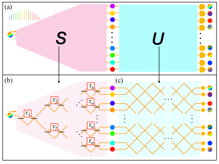
Figure 1: (a) High-dimensional frequency-encoded unitary transformation and projection measurement with passive photonic circuit and time-resolving detection. Different colors indicate different frequency modes, and the gradient color shows a superposition of multiple frequency modes. (b) Photonic circuit to realize S for a quantum frequency comb with evenly distributed frequency modes, $\tau_{j}=\pi/(2^{(j-1)}\delta\omega)$. (c) Photonic circuit to realize unitary transformation U.

In contrast to traditional methods utilizing nonlinear optical processes to build frequency-domain beam splitters, we show that these operations can be realized with passive photonic circuits and time-resolving detection [Fig. 1(a)]. First, discrete frequency modes are associated with different spatial modes through operator S, which can practically be realized by a prism, optical grating, or Mach-Zehnder interferometer (MZI) array

$$\textbf{S}|\psi\rangle=\sum_{k=0}^{N-1}c_{k}\hat{a}^{\dagger}_{\omega_{k},r_{k}}|0\rangle^{\otimes N^{2}}$$ (2)

where $r_{k}$ is the spatial mode that carries the $\omega_{k}$ frequency component. For a quantum frequency comb with evenly distributed frequency modes, one possible design of the passive photonic circuit is shown in Fig. 1(b). For the case the frequency mode number $N=2^{n}$ with $n$ a positive integer, the operator S can be realized with $2^{n}-1$ unbalanced MZIs Huntington et al. (2005) arranged hierarchically into $n$ levels [Fig. 1(b)]. For the $j$th level, the relative time delay of the MZIs is set to be $\tau_{j}=\pi/(2^{(j-1)}\delta\omega)$, with $\delta\omega$ the free-spectral range of the quantum frequency comb Com . For the case $2^{n-1}<N<2^{n}$, the same circuit can be used and the redundant modes can be dropped. Then the $N$ spatial modes are sent into an $N$-port passive photonic circuit to realize unitary transformation U in a spatial domain Reck et al. (1994); Clements et al. (2016); Zhang et al. (2019). Since spatial modes simultaneously represent frequency modes, the interference in a spatial domain also results in mixing of associated frequency modes

$$\textbf{U}~{}\hat{a}^{\dagger}_{\omega_{k},r_{k}}=\sum_{j=0}^{N-1}u_{jk}\hat{a}^{(\text{out}){\dagger}}_{\omega_{k},r_{j}}$$ (3)

where $r_{j}$ indicates the $j$th output spatial mode of the photonic circuit [Fig. 1(c)]. Then the output spatial modes are measured with ultrafast detectors. The outcome of $j$th output port is expressed as

$$P_{j}(t;T)= \int^{t+T/2}_{t-T/2}\frac{d\tau}{T}~{}\langle\psi|\textbf{S}^{\dagger}\textbf{U}^{\dagger}\hat{E}^{{\dagger}}_{r_{j}}(\tau)\hat{E}_{r_{j}}(\tau)\textbf{U}\textbf{S}|\psi\rangle$$ (4)

$$= \int^{t+T/2}_{t-T/2}\frac{d\tau}{T}~{}\langle\psi|e^{i\hat{H}\tau/\hbar}\textbf{M}_{j}e^{-i\hat{H}\tau/\hbar}|\psi\rangle$$

$$= \int^{t+T/2}_{t-T/2}\frac{d\tau}{T}~{}\langle\psi|\textbf{M}_{j}(\tau)|\psi\rangle$$

with $T$ the detector’s response time, $\hat{H}=\sum_{k=0}^{N-1}\hbar\omega_{k}(\hat{a}^{\dagger}_{\omega_{k}}\hat{a}_{\omega_{k}}+\frac{1}{2})$, and $\hat{E}_{r_{j}}(\tau)=\sum_{k=0}^{N-1}\hat{a}^{(\text{out})}_{\omega_{k},r_{j}}e^{-i\omega_{k}\tau}$, representing the equivalent photon phase change due to detection jitter. With infinitely small $T$, the measurement outcome in a spatial domain approaches the desired projection measurement in a frequency domain.

$$\lim_{T\rightarrow 0^{+}}P_{j}(t;T)=\text{Tr}(\textbf{M}_{j}|\psi\rangle\langle\psi|)$$ (5)

Therefore, the complete set of projection operators in a frequency domain can be realized with passive photonic circuits and time-resolving detection. This approach is based on the Fourier correspondence between frequency and temporal correlations Pe’Er et al. (2005); O’Donnell (2011); Lukens et al. (2013); Bernhard et al. (2013).

Considering the practical condition of detector’s finite response time, the fidelity of the projection measurement can be expressed as

$$F_{j}=\dfrac{\left|\text{Tr}\left(\widetilde{\textbf{M}}_{j}(t;T)^{\dagger}\textbf{M}_{j}\right)\right|^{2}}{\text{Tr}(\widetilde{\textbf{M}}_{j}(t;T)^{\dagger}\widetilde{\textbf{M}}_{j}(t;T))\text{Tr}(\textbf{M}_{j}^{\dagger}\textbf{M}_{j})}$$ (6)

with $\widetilde{\textbf{M}}_{j}(t;T)=\int^{t+T/2}_{t-T/2}\frac{d\tau}{T}\textbf{M}_{j}(\tau)$ the effective projection.

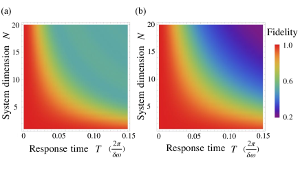
Figure 2: The measurement fidelity with finite response time $T$ and dimension $N$ when the projection measurement is onto (a) the two-mode superposition with largest frequency difference $1/\sqrt{2}(\hat{a}^{\dagger}_{\omega_{0}}+\hat{a}^{\dagger}_{\omega_{0}+(N-1)\delta\omega})|0\rangle^{\otimes N}$ and (b) the Fourier basis $1/\sqrt{N}\sum_{k=0}^{N-1}\hat{a}^{\dagger}_{\omega_{0}+k\delta\omega}|0\rangle^{\otimes N}$.

Practically, the system’s total response time $T$ is dominated by phase instability in the photonic circuit or detector jitter. A large response time will inevitably degrade the fidelity of projection measurement (Fig. 2). In order to achieve high-fidelity operation, the response time needs to be much smaller than the beating period of the quantum frequency comb, $T<<2\pi/\delta\omega$. In addition, the fidelity of projection measurement with different bases have different dependencies on the response time $T$. The projection onto the basis with fast temporal evolution, such as two-mode superposition with large frequency difference [Fig. 2(a)] and the Fourier basis [Fig. 2(b)], will be more sensitive to the error induced by the finite response time. In contrast, the fidelity of the projection measurement onto the computational basis with single frequency modes will not be influenced.

With the capability to realize arbitrary projection measurement, we further develop the approach to verify bipartite high-dimensional quantum entanglement encoded in a frequency domain with passive photonic circuits and time-resolving detection Kaszlikowski et al. (2000); Daniel et al. (2002). Two sets of projection bases, time-delayed Fourier basis and time-delayed inverse Fourier basis, can be defined for photon $a$ and $b$, respectively.

$$|M {}_{a,j}(t)\rangle$$ (7)

$$=\frac{1}{\sqrt{N}}\sum_{k=0}^{N-1}\exp\left\{i\left(\frac{2\pi j}{N}+\delta\omega t\right)k\right\}\hat{a}^{\dagger}_{\omega_{k}}|0\rangle^{\otimes N}$$

$$|M {}_{b,j}(t)\rangle$$

$$=\frac{1}{\sqrt{N}}\sum_{k=0}^{N-1}\exp\left\{i\left(-\frac{2\pi j}{N}+\delta\omega t\right)k\right\}\hat{b}^{\dagger}_{\omega_{N-1-k}}|0\rangle^{\otimes N}$$

where integer $j$ labels the index of output port. Both sets of projection measurement can be realized with the photonic circuits shown in Fig. 1. The generalized high-dimensional entanglement indicator can be written as

$$S_{N}(t_{a},t_{b},t^{\prime}_{a},t^{\prime}_{b})\overset{\text{\tiny def}}{=}\sum_{k=0}^{[N/2]-1} (1-\frac{2k}{N-1})\{[P(t_{a},t_{b},k)+P(t^{\prime}_{a},t_{b},-k-1)+P(t^{\prime}_{a},t^{\prime}_{b},k)+P(t_{a},t^{\prime}_{b},-k)]$$ (8)

$$-[P(t_{a},t_{b},-k-1)+P(t^{\prime}_{a},t_{b},k)+P(t^{\prime}_{a},t^{\prime}_{b},-k-1)+P(t_{a},t^{\prime}_{b},k+1)]\}$$

$$P(t_{a},t_{b},k)=\frac{1}{T^{2}}\iint_{-T/2}^{T/2}dtdt^{\prime}\sum_{l=0}^{N-1}|\langle M_{a,l}(t_{a}+t),M_{b,(l+k)\text{mod}d}(t_{b}+t^{\prime})|\psi\rangle|^{2}$$ (9)

with $t_{a}$, $t^{\prime}_{a}$ and $t_{b}$, $t^{\prime}_{b}$ corresponding to different settings of the photonic circuits, thus different projections bases, for photon $a$ and $b$, respectively Daniel et al. (2002). Classically, the maximum value of $S_{N}$ is 2. The quantum limit of $S_{N}$, which is above 2, can be achieved with the high-dimensional Bell state

$$|\psi\rangle=\frac{1}{\sqrt{N}}\sum_{k=0}^{N-1}\hat{a}^{\dagger}_{\omega_{k}}\hat{b}^{\dagger}_{\omega_{N-1-k}}|00\rangle^{\otimes N}.$$ (10)

by setting the detection time $t_{b}-t_{a}=\frac{\pi}{2N\delta\omega}$ and $t^{\prime}_{a}-t_{a}=t^{\prime}_{b}-t_{b}=\frac{\pi}{N\delta\omega}$.

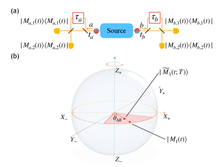
Figure 3: (a) Setup to verify two-frequency bipartite entanglement. (b) Bloch sphere for two-frequency systems. Red shaded area is the time averaging range with the designed and equivalent measurement shown as arrows.

While the exact value of $S_{N}$ is dependent on the size $N$ of high-dimensional systems Daniel et al. (2002), we use the two-frequency case as an example to illustrate our approach and the effect of a finite response time. In two-frequency systems, the photonic circuits shown in Fig. 1 can be simplified to a single unbalanced MZI for each photon [Fig. 3(a)], and the corresponding projection basis can be represented on Bloch sphere [Fig. 3(b)]. With two frequency modes $\omega_{1}$ and $\omega_{2}$, the criterion for quantum entanglement can be simplified to the CHSH inequality, which can be maximally violated with the Bell state

$$|\psi\rangle=\frac{1}{\sqrt{2}}(\hat{a}^{\dagger}_{\omega_{1}}\hat{b}^{\dagger}_{\omega_{2}}+\hat{a}^{\dagger}_{\omega_{2}}\hat{b}^{\dagger}_{\omega_{1}})|00\rangle^{\otimes N}$$ (11)

By setting both relative delay $\tau_{a}$ and $\tau_{b}$ giving $\pi/2$ and -$\pi/2$ phase difference for mode $\omega_{1}$ and $\omega_{2}$ respectively Com , the projection bases are placed on the equator of the Bloch sphere,

$$|M_{c,j}(t)\rangle=\frac{1}{\sqrt{2}}(\hat{c}^{\dagger}_{\omega_{1}}+(-1)^{j}e^{i\delta\omega t_{c}}\hat{c}^{\dagger}_{\omega_{2}})|0\rangle^{\otimes N}$$ (12)

where subscripts $\hat{c}=\hat{a},\hat{b}$ and $j=1,2$ label the photon and measurement output, respectively. Photon clicks at output 1 and 2 correspond to $+1$ and $-1$ in the original CHSH scheme respectivley Aspect et al. (1982); Rarity and Tapster (1990); Ou et al. (1990). Then the CHSH value can be defined through the correlation coefficient $E(t_{a},t_{b})$ and the coincidence rate $\bar{C}_{ij}(t_{a},t_{b})$

$$S_{2}=E(t_{a},t_{b})-E(t_{a},t^{\prime}_{b})+E(t^{\prime}_{a},t_{b})+E(t^{\prime}_{a},t^{\prime}_{b})$$ (13)

$$E(t_{a},t_{b})=\dfrac{\bar{C}_{11}(t_{a},t_{b})+\bar{C}_{22}(t_{a},t_{b})-\bar{C}_{12}(t_{a},t_{b})-\bar{C}_{21}(t_{a},t_{b})}{\bar{C}_{11}(t_{a},t_{b})+\bar{C}_{22}(t_{a},t_{b})+\bar{C}_{12}(t_{a},t_{b})+\bar{C}_{21}(t_{a},t_{b})}$$

$$\bar{C}_{ij}(t_{a},t_{b})\propto\frac{1}{T^{2}}\iint_{-T/2}^{T/2}dtdt^{\prime}|\langle M_{a,i}(t_{a}+t),M_{b,j}(t_{b}+t^{\prime})|\psi\rangle|^{2}$$

The maximum value of $S_{2}$ is achieved when photon detection time satisfies $t_{b}-t_{a}=\frac{\pi}{4\delta\omega}$, $t^{\prime}_{a}-t_{a}=\frac{\pi}{2\delta\omega}$ and $t^{\prime}_{b}-t_{b}=\frac{-\pi}{2\delta\omega}$. These conditions correspond to fixing the angle between projection bases for photon $a$ and $b$ to be 45 degree, and the bases are rotated by 90 degree along the Z-axis of the Bloch sphere between the two measurements. The finite response time will inevitably degrade the measurement results. In this particular setup, the effect of the finite response time corresponds to averaging along an arc on the the Bloch sphere equator [Fig. 3(b)]. And the angle of the arc is equal to $T\cdot\delta\omega$. The calculated result of $S_{2}$ with fixed optimum $t^{\prime}_{a}-t_{a}$, $t^{\prime}_{b}-t_{b}$ and varying $t_{b}-t_{a}$ values is shown in Fig. 4(a). The violation of the classical limit of $S_{2}$ is clearly observed with a small response time. And the theoretical limit $2\sqrt{2}$ can be achieved with a infinitely small response time. With a larger response time, the measured maximal $S_{2}$ decreases [Fig. 4(a)]. When the response time is larger than the threahold value $T_{0}$ with $\text{sinc}^{2}(\delta\omega T_{0}/2)=1/\sqrt{2}$ corresponding to $T_{0}\approx 0.32\times(2\pi/\delta\omega)$, the maximal measurable value of $S_{2}$ falls below the classical limit, meaning the quantum correlation cannot be distinguished. Here, we assume unity detection efficiency. Lower efficiency will inevitably limits the overall projection measurement efficiency and decrease signal-to-noise ratio in experiments. For certain applications, such as loop-hole free CHSH test Giustina et al. (2013); Christensen et al. (2013), overal efficiency above certain threshold will be required.

Discussion and Outlook.—In addition to eliminating nonlinear optical processes, another major advantage of our approach is scalability. From a theoretical perspective, the systematic approach to design photonic circuit for a quantum frequency comb with an arbitrary large size has been carried out as shown in Fig. 1. From the experimental perspective, the complete photonic circuit can be robustly fabricated on nanophotonic platforms such as silicon and silicon nitride at large scale with standard CMOS technology Politi et al. (2009). Such a photonic circuit can also be conveniently tuned through thermal-optic effect to realize different projection bases  Politi et al. (2009). Moreover, superconducting single photon detectors have been integrated on various nanophotonic circuits with high efficiency and low jitter Pernice et al. (2012); Schuck et al. (2016). Therefore, our approach can be scalable fabricated with complete integrated quantum photonic platforms. Extra caution should be taken to minimize the frequency dependence of unitary $U$. One possible approach is to design phase shifters using waveguides with length $L=\frac{2\pi c}{n_{g}\delta\omega}$ and near-zero dispersion. Furthermore, the achievable length of optical delay line with nanophotonic circuits limits the frequency resolution of the circuits. Currently, nanophotonic optical delay line with length above 30 m and loss below 0.08 dB/m has been demonstrated  Lee et al. (2012), leading to frequency resolution well below 1 GHz.

While fidelity of processing frequency-encoded quantum states with our approach depends critically on the response time, the major limiting factor is the detector jitter. Currently, superconducting single photon detectors have achieved a jitter time below 3 ps, with a theoretical limit below 1 ps Korzh et al. (2018); Allmaras et al. (2019). Current jitter performance is enough to maintain fidelity above 90% for an 85-mode free-space quantum frequency comb, with free spectral range normally below 1 GHz. The maximum frequency range that can preserve quantum effect is determined by the two-mode CHSH test, $\delta\omega/2\pi\approx 0.32/T\approx$100 GHz, which is accessible by most integrated photonic platforms.

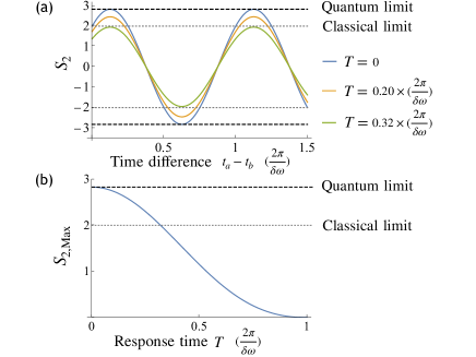
Figure 4: (a) CHSH quantity $S_{2}$ values with varying detection time difference $t_{a}-t_{b}$ and fixed $\tau_{a}$ and $\tau_{b}$. (b) Maximal measurable $S_{2,{\text{Max}}}$ with dependence on response time $T$.

Finally, a few remarks are in order on potential uses of our proposed method for continuous-variable (CV) photonic quantum information processing. While our derivation is based on single-photon state, the extension to arbitrary multiphoton input states with photon-number-resolving (PNR) detectors is straightforward. This is of critical importance for CV quantum information processing. One possible application with high impact will be Gaussian-Boson-Sampling (GBS) Hamilton et al. (2017). We start with N-mode CV Gaussian quantum frequency comb generated with an optical parametric oscillator (OPO), and use our proposed method to implement projection measurement with fast PNR detection on all output ports. In this case, GBS can be realized in frequency domain with very compact device and high efficiency Pfister (2019); Menicucci et al. (2006); Weedbrook et al. (2012).

In conclusion, we have proposed a novel approach to realize high-dimensional quantum information processing encoded in photon frequency domain with passive photonic circuit and time-resolving detection. This approach features no active nonlinear optical process, high scalability, and no intrinsic loss. The capability to process high-dimensional frequency-encoded quantum photonic states can be dramatically improved, benefiting critical quantum applications including cluster-model quantum computing Zhou et al. (2003), high-dimensional quantum correlation verification Kaszlikowski et al. (2000); Daniel et al. (2002), and high-efficiency Boson sampling Laibacher and Tamma (2018).

References

- O’brien et al. (2009) J. L. O’brien, A. Furusawa, and J. Vučković, Nature Photonics 3, 687 (2009).
- Gisin and Thew (2007) N. Gisin and R. Thew, Nat. Photonics 1, 165 (2007).
- Pirandola et al. (2018) S. Pirandola, B. R. Bardhan, T. Gehring, C. Weedbrook, and S. Lloyd, Nat. Photonics 12, 724 (2018).
- Weedbrook et al. (2012) C. Weedbrook, S. Pirandola, R. García-Patrón, N. J. Cerf, T. C. Ralph, J. H. Shapiro, and S. Lloyd, Reviews of Modern Physics 84, 621 (2012).
- Zhou et al. (2003) D. Zhou, B. Zeng, Z. Xu, and C. Sun, Phys. Rev. A 68, 062303 (2003).
- Lanyon et al. (2009) B. P. Lanyon, M. Barbieri, M. P. Almeida, T. Jennewein, T. C. Ralph, K. J. Resch, G. J. Pryde, J. L. O’brien, A. Gilchrist, and A. G. White, Nat. Phys. 5, 134 (2009).
- Babazadeh et al. (2017) A. Babazadeh, M. Erhard, F. Wang, M. Malik, R. Nouroozi, M. Krenn, and A. Zeilinger, Phys. Rev. Lett. 119, 180510 (2017).
- (8) The number of qudits and dimension determines the computational power of a quantum processor together. Increasing makes the dimension of Hilbert space scale exponentially while increasing scales in polynomial.
- Kues et al. (2019) M. Kues, C. Reimer, J. M. Lukens, W. J. Munro, A. M. Weiner, D. J. Moss, and R. Morandotti, Nat. Photonics 13, 170 (2019).
- Pfister (2019) O. Pfister, J. Phys. B 53, 012001 (2019).
- Cundiff and Ye (2003) S. T. Cundiff and J. Ye, Reviews of Modern Physics 75, 325 (2003).
- Gaeta et al. (2019) A. L. Gaeta, M. Lipson, and T. J. Kippenberg, Nature Photonics 13, 158 (2019).
- Chen et al. (2014) M. Chen, N. C. Menicucci, and O. Pfister, Phys. Rev. Lett. 112, 120505 (2014).
- Pinel et al. (2012) O. Pinel, P. Jian, R. M. De Araujo, J. Feng, B. Chalopin, C. Fabre, and N. Treps, Phys. Rev. Lett. 108, 083601 (2012).
- Xie et al. (2015) Z. Xie, T. Zhong, S. Shrestha, X. Xu, J. Liang, Y.-X. Gong, J. C. Bienfang, A. Restelli, J. H. Shapiro, F. N. Wong, et al., Nat. Photonics 9, 536 (2015).
- Reimer et al. (2016) C. Reimer, M. Kues, P. Roztocki, B. Wetzel, F. Grazioso, B. E. Little, S. T. Chu, T. Johnston, Y. Bromberg, L. Caspani, et al., Science 351, 1176 (2016).
- Kues et al. (2017) M. Kues, C. Reimer, P. Roztocki, L. R. Cortés, S. Sciara, B. Wetzel, Y. Zhang, A. Cino, S. T. Chu, B. E. Little, et al., Nature 546, 622 (2017).
- Imany et al. (2018) P. Imany, J. A. Jaramillo-Villegas, O. D. Odele, K. Han, D. E. Leaird, J. M. Lukens, P. Lougovski, M. Qi, and A. M. Weiner, Opt. Express 26, 1825 (2018).
- Clemmen et al. (2016) S. Clemmen, A. Farsi, S. Ramelow, and A. L. Gaeta, Phys. Rev. Lett. 117, 223601 (2016).
- Lu et al. (2018) H.-H. Lu, J. M. Lukens, N. A. Peters, O. D. Odele, D. E. Leaird, A. M. Weiner, and P. Lougovski, Phys. Rev. Lett. 120, 030502 (2018).
- Lukens and Lougovski (2017) J. M. Lukens and P. Lougovski, Optica 4, 8 (2017).
- Huntington et al. (2005) E. Huntington, G. Milford, C. Robilliard, T. Ralph, O. Glöckl, U. L. Andersen, S. Lorenz, and G. Leuchs, Physical Review A 71, 041802 (2005).
- (23) The design shown in Fig 1b assumes that the center frequency is a multiple of the free-spectral-range , which is true for an optical cavity with zero dispersion. For a more general case where is not a multiple of , we could set a minimum frequency resolution , and a natural choice would be the linewidth of frequency modes. Therefore, we can always find a pair of coprime integer and and two frequency detunings and , that satisfy with and . Therefore, the time delay for MZIs at th level is changed to , which can separate different frequency modes into different paths within the resolution.
- Reck et al. (1994) M. Reck, A. Zeilinger, H. J. Bernstein, and P. Bertani, Phys. Rev. Lett. 73, 58 (1994).
- Clements et al. (2016) W. R. Clements, P. C. Humphreys, B. J. Metcalf, W. S. Kolthammer, and I. A. Walmsley, Optica 3, 1460 (2016).
- Zhang et al. (2019) C. Zhang, J. Chen, C. Cui, J. P. Dowling, Z. Ou, and T. Byrnes, Phys. Rev. A 100, 032330 (2019).
- Pe’Er et al. (2005) A. Pe’Er, B. Dayan, A. A. Friesem, and Y. Silberberg, Phys. Rev. Lett. 94, 073601 (2005).
- O’Donnell (2011) K. A. O’Donnell, Phys. Rev. Lett. 106, 063601 (2011).
- Lukens et al. (2013) J. M. Lukens, A. Dezfooliyan, C. Langrock, M. M. Fejer, D. E. Leaird, and A. M. Weiner, Phys. Rev. Lett. 111, 193603 (2013).
- Bernhard et al. (2013) C. Bernhard, B. Bessire, T. Feurer, and A. Stefanov, Phys. Rev. A 88, 032322 (2013).
- Kaszlikowski et al. (2000) D. Kaszlikowski, P. Gnaciński, M. Żukowski, W. Miklaszewski, and A. Zeilinger, Phys. Rev. Lett. 85, 4418 (2000).
- Daniel et al. (2002) C. Daniel, N. Gisin, N. Linden, S. Massar, and S. Popescu, Phys. Rev. Lett. 88, 040404 (2002).
- Aspect et al. (1982) A. Aspect, P. Grangier, and G. Roger, Phys. Rev. Lett. 49, 91 (1982).
- Rarity and Tapster (1990) J. Rarity and P. Tapster, Phys. Rev. Lett. 64, 2495 (1990).
- Ou et al. (1990) Z. Ou, X. Zou, L. Wang, and L. Mandel, Phys. Rev. Lett. 65, 321 (1990).
- Giustina et al. (2013) M. Giustina, A. Mech, S. Ramelow, B. Wittmann, J. Kofler, J. Beyer, A. Lita, B. Calkins, T. Gerrits, S. W. Nam, et al., Nature 497, 227 (2013).
- Christensen et al. (2013) B. Christensen, K. McCusker, J. Altepeter, B. Calkins, T. Gerrits, A. E. Lita, A. Miller, L. K. Shalm, Y. Zhang, S. Nam, et al., Phys. Rev. Lett. 111, 130406 (2013).
- Politi et al. (2009) A. Politi, J. C. Matthews, M. G. Thompson, and J. L. O’Brien, IEEE Journal of Selected Topics in Quantum Electronics 15, 1673 (2009).
- Pernice et al. (2012) W. H. Pernice, C. Schuck, O. Minaeva, M. Li, G. Goltsman, A. Sergienko, and H. Tang, Nature communications 3, 1325 (2012).
- Schuck et al. (2016) C. Schuck, X. Guo, L. Fan, X. Ma, M. Poot, and H. X. Tang, Nature communications 7, 10352 (2016).
- Lee et al. (2012) H. Lee, T. Chen, J. Li, O. Painter, and K. J. Vahala, Nat. Commun 3, 867 (2012).
- Korzh et al. (2018) B. Korzh, Q. Zhao, S. Frasca, J. Allmaras, T. Autry, E. Bersin, M. Colangelo, G. Crouch, A. Dane, T. Gerrits, et al., arXiv preprint arXiv:1804.06839 (2018).
- Allmaras et al. (2019) J. P. Allmaras, A. G. Kozorezov, B. A. Korzh, K. K. Berggren, and M. D. Shaw, Phys. Rev. Appl. 11, 034062 (2019).
- Hamilton et al. (2017) C. S. Hamilton, R. Kruse, L. Sansoni, S. Barkhofen, C. Silberhorn, and I. Jex, Physical review letters 119, 170501 (2017).
- Menicucci et al. (2006) N. C. Menicucci, P. Van Loock, M. Gu, C. Weedbrook, T. C. Ralph, and M. A. Nielsen, Physical review letters 97, 110501 (2006).
- Laibacher and Tamma (2018) S. Laibacher and V. Tamma, arXiv preprint arXiv:1801.03832 (2018).