Peierls versus Holstein models for describing electron-phonon coupling in perovskites

Abstract

We use the Momentum Average approximation together with perturbative approaches, in the appropriate limits, to study the single polaron physics on a perovskite lattice inspired by BaBiO₃. We investigate electron-phonon coupling of the Peierls type whereby the motion of ions modulates the values of the hopping integrals between sites, and show that it cannot be mapped onto the simpler one-band Holstein model in the whole parameter space. This is because the dispersion of the Peierls polaron has sharp transitions where the ground-state momentum jumps between high-symmetry points in the Brillouin zone, whereas the Holstein polaron always has the same ground-state momentum. These results imply that careful consideration is required to choose the appropriate model for carrier-lattice coupling in such complex lattices.

I Introduction

Materials with perovskite structure ABO₃ are known to have a wide variety of extraordinary properties, ranging from unconventional high-temperature superconductivity in cuprates,Gao et al. (1994); Presland et al. (1991); Tallon et al. (1995); Obertelli et al. (1992) to an unusual metal-to-insulator transition in rare-earth nickelates, Subedi et al. (2015) to colossal magneto-resistance in manganites, Srivastava et al. (2009); Abdelkhalek et al. (2011) to multiferroic behaviour, Liu and Yang (2017) among others.

Many of these properties are believed to arise from the interplay of charge, spin, orbital and lattice degrees of freedom and of their various interactions. A full detailed treatment of all this complexity is still unfeasible, resulting in the urgent need to identify simpler but useful models. For instance, is it ever necessary to consider the full multiplet structure for rare-earths with partially filled $3d$ levels, or does it suffice to include explicitly only one/few of them, with a simplified description for correlations? One well-known example where this kind of question is relevant are the cuprates, where most models only consider the $3d_{x^{2}-y^{2}}$ orbital for Cu.Anderson (1987); Emery (1987); Jiang et al. (2020) Even more basic is the question of which of the constituent elements need to be included in the modelling. To continue with the CuO₂ layer example, even though it is well known that the doped holes are on the anions, most models do not explicitly included the oxygen ions. Another example are the rare-earth nickelates, where only recently it has become clear how essential it is to include the O explicitly in the models.Johnston et al. (2014); Park et al. (2012) Of course, the answers will vary from one material to another, but it is important to ask such questions and to understand when certain approximations may be valid, and when they are certainly not.

From this perspective, the modeling of the electron-phonon coupling in perovskites may appear to be on better footing than other issues, as it has been very customary to use a Holstein coupling to describe it. Pankaj and Yarlagadda (2012); Kurdestany and Satpathy (2017) The Holstein model Holstein (1959) is the simplest possible description of charge carriers interacting with phonons on a lattice. It was proposed for “molecular crystals”, with the Einstein mode describing not lattice phonons, but instead an internal deformation of the individual molecules when an additional carrier is present. As such, it is not at all obvious that a Holstein description is appropriate for a complicated system like a perovskite. Part of the reason for using it is that earlier studies of several electron-phonon couplings (Holstein,Holstein (1959) Fröhlich,Fröhlich et al. (1950), breathing-mode,Kurzynski (1976); Lau et al. (2007); Goodvin and Berciu (2008) etc.) on simple lattices revealed qualitatively similar behavior Alexandrov (2008), suggesting that using the simplest model is likely appropriate. This idea was backed up for perovskites, under certain assumptions, for a more detailed model discussed below. Our work challenges this view.

At this point, we must note that an issue that has caused confusion regarding the importance of electron-phonon coupling, especially in perovskite structures like the nickelates, the high-T_C cuprates, the weakly correlated BaBiO₃ and also other systems, is the weak electron-phonon coupling obtained with ab-initio methods like the Density Functional Theory (DFT). For example, electron-phonon coupling in cuprates extracted from DFT was deemed much too small to generate a strong enough pairing for high-T_c superconductivity.Savrasov and Andersen (1996) However, this is based on DFT results that predict the $3d_{x^{2}-y^{2}}$ bandwidth to be close to 4 eV, whereas because of the strongly correlated nature of the Cu $3d$ electrons, the bandwidth of the so-called Zhang-Rice singletZhang and Rice (1988) band is only about 0.3 eV wide.Yin et al. (2008) This bandwidth renormalization increases the effective electron-phonon coupling to the relevant electronic states by an order of magnitude. This was also noted by Khalliulin and Horsch in their estimate of a dimensionless effective coupling $\lambda=0.25$. Khaliullin and Horsch (1997) At the opposite end of the spectrum, we note that that interpretation of the ARPES data on Sr₂CuO₂Cl₂ in terms of polaron formationShen et al. (2004) leads to an extremely strong effective coupling of $\lambda\approx 6.25$. Goodvin (2009)

To make the discussion specific, from now on we will use the perovskite BaBiO₃ as our inspiration. This is a good choice because (i) here there are no complications from strong correlations and/or spin-orbit coupling (for reasons detailed in the next section), and (ii) electron-phonon coupling is believed to be strong in this material, and in fact K-doped BaBiO₃ has a record high $T_{C}\approx 35$K for a superconductor with a phonon glue. The reason for this high value of $T_{C}$ is not yet fully settled. Again, conventional DFT results predict a much too weak coupling, Hamada et al. (1989); Shirai et al. (1990); Liechtenstein et al. (1991); Kunc and Zeyher (1994); Meregalli and Savrasov (1998); Bazhirov et al. (2013) but a more local molecular-like description of the electronic structure yields a very substantial electron-phonon coupling, with a $\lambda\sim 1$.Khazraie et al. (2018a)

There have already been lots of studies of this very interesting material. For example, the Rice-Sneddon model described below is widely used Kostur and Allen (1997); Allen and Kostur (1997); Piekarz and Konior (2000); Bischofs et al. (2002) to investigate the formation and properties of polarons and bipolarons in BaBiO₃. It has been argued that it maps accurately onto an effective single band Holstein model,Nourafkan et al. (2012) which was then used to study the optical properties of BaBiO₃ and the metal-insulator transition in hole-doped BaBiO₃. Seibold and Sigmund (1993)

In this work, we challenge this well-established view that a one-band Holstein model always provides a good description (at least qualitatively, if not quantitatively) of the electron-phonon coupling in perovskites. Our starting point is a Peierls model that explicitly includes the O sites and takes into consideration the significant modulation of the hopping between Bi and O, when the lighter O ions vibrate. This type of coupling is ignored by the Rice-Sneddon model, which instead focusses on the change of the on-site energy of the carrier when on a Bi ion, because of the deformation of the O cage surrounding it.

We are unable to provide accurate results in the physically relevant limit of half-filling, i.e. when there is one hole per unit cell. Instead, we consider the extreme case when there is a single hole in the entire system (effectively zero carrier concentration, for an infinite lattice), because here we can study the properties of the resulting polaron sufficiently accurately to draw unequivocal conclusions. Moreover, we investigate the behavior of our model in the wider parameter space, including regions that are far from where BaBiO₃ is expected to be located. This is partially due to technical reasons, as the variational approximation that we employ becomes more accurate for phonon frequencies similar to, or larger than the electronic intersite hopping integral. As we will show, the behavior of interest to us appears to evolve smoothly with decreasing phonon frequencies, so some inferrences can be made about what happens in the adiabatic limit. Nevertheless, it is important to find other methods that are reliable in this limit, to verify our conclusions there. A separate reason to study models with relatively narrow bandwidths, is the concerted effort in modern condensed matter physics to develop so-called “flat-band” materials, like twisted graphene or ordered impurity-based midgap bands in semiconductors or insulators. In such materials, the effective bandwidths can be comparable to or smaller than the phonon frequencies, and our results would be directly relevant to them.

Our results demonstrate that in certain regions of the parameter space, the Peierls model on a perovskite lattice exhibits single polaron behavior that is impossible to reproduce with a Holstein model. Specifically, as the electron-phonon coupling is increased, the polaron dispersion changes its shape such that the ground-state momentum switches from its free-carrier value to another high-symmetry point in the Brillouin zone. Such sharp transitions are impossible for a Holstein polaron.Gerlach and Löwen (1991)

Based on this result, we conclude that the Peierls model cannot be automatically replaced with a Holstein model when studying a perovskite system.

This being said, it is important to emphasize the caveat that our study is in the single-polaron limit. It is possible that at finite carrier concentration, the mapping between Peierls and Holstein couplings might be valid for some other reasons – however, this has to be explicitly verified and not just assumed. To the best of our knowledge, there is no work addressing this question. We also emphasize that there are regions of the parameter space (including the region where BaBiO₃ is believed to be located) where the polaron ground-state momentum equals the free-carrier value, and therefore a Holstein model may be sufficient to mimic the polaron behavior for a correct choice of effective parameters. Again, our point is that this is not automatically the case for all perovskite materials, therefore care is needed and one must do detailed work to justify the use of a Holstein model as a reasonable description of the electron-phonon coupling.

The paper is organized as follows: in Section II we introduce our model, in Section III we describe the various methods we used to study it, and in Section IV we present the results. Section V contains the discussion and conclusions. Technical details are relegated to Appendices.

II Model

We use the following approximations to model the generic perovskite ABO₃:

(i) sites A are taken to be irrelevant for the physics of interest to us, and are ignored. Physically, this implies that electronic bands with dominant A-character are lying well below and/or well above the Fermi energy. For BaBiO₃, which is our main inspiration, this is a good approximation. It reduces the lattice of interest from a full perovskite to the BO₃ lattice sketched in Fig. 1a.

(ii) For the B sites, the relevant electronic orbital is non-degenerate and spatially well spread out, so that the on-site Hubbard repulsion can be safely ignored. This is a good approximation for BaBiO₃, where this is the Bi:$6s$ orbital. From now we will call this the “s”-orbital, and denote by $s_{i,\sigma}^{\dagger}$ the creation operator for a hole with spin $\sigma$ in this orbital of the atom B in the unit cell $i$.

(iii) At each O site, we only keep in the model the $2p_{\gamma}$ orbital with ligand character, i.e. $\gamma=x,y,z$ for the O located on bonds parallel to $x,y,z$, respectively. We will refer to this as the $x,y$ or $z$ orbital, and use either the generic $\gamma^{\dagger}_{i,\sigma}$ operator when refering to any of the three O in the unit cell $i$, or the specific $x^{\dagger}_{i,\sigma},y^{\dagger}_{i,\sigma},z^{\dagger}_{i,\sigma}$ for the creation operator associated with adding a hole to the O located on the $x,y,z$ bond of unit cell $i$, see Fig. 1(b).

(iv) We ignore all phonon modes that are primarily located on A and B sites, and instead keep only the optical phonon describing longitudinal (parallel to its ligand bond) oscillations of each O. The first part is reasonable as the A and B atoms are much heavier than O, so we expect their motion to mostly contribute to very low-energy phonon modes which do not couple strongly to the hole’s motion (see below). The second part is justified because to first order, one can think of each O as oscillating longitudinally between its two immobile B neighbours, with a characteristic frequency $\Omega$ that is the same at all O sites. For a crystal, this is equivalent with an Einstein phonon mode of frequency $\Omega$ on the O sites. In the following, we will denote the phonon creation operator for the $\gamma=\{x,y,z\}$ O site in unit cell $i$ as $b^{\dagger}_{i,\gamma}$.

In this work, we focus on the effect of this phonon mode on the hybridization between neighbor O and B sites, as well as neighbor O sites. The resulting electron-phonon coupling is known as a Peierls coupling, and should be contrasted to the Rice-Sneddon model that focuses on the modulation of the on-site energy of a hole located in the $s$-orbital, due to oscillatory motion of adjacent O. As discussed in the Introduction, the latter has been argued to be well modelled by an effective Holstein coupling on a simplified cubic lattice with only $B$ sites included. Our results discussed below show that this equivalence with a Holstein model does not hold for the Peierls coupling in a considerable region of the parameter space.

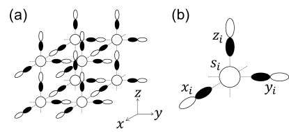
Figure 1: (a) Sketch of the model for an infinite 3D lattice, showing $s$ orbitals at the B sites, and the ligand $2p$ orbitals at the O sites. The A sites are ignored. (b) Our choice for the unit cell $i$ has an $s$-orbital labeled by $s_{i}$ and three $2p$-orbitals labeled $x_{i}$, $y_{i}$ and $z_{i}$ along the three ligand bonds.

To summarize, the Peierls model that we study is:

$$\hat{H}=\hat{H_{0}}+\hat{V},$$ (1)

where

$$\hat{H_{0}}=\Omega\sum_{i,\gamma}b^{\dagger}_{i\gamma}b_{i\gamma}-\Delta\sum_{i,\gamma}\gamma^{\dagger}_{i}\gamma_{i}+T_{sp}+T_{pp}$$ (2)

describes the Einstein phonon modes (we set $\hbar=1$), the charge-transfer energy $\Delta$ between $p$ and $s$ atomic orbitals, and the nearest neighbor (nn) $s$-$p$ and $p$-$p$ hopping, respectively, while

$$\hat{V}=H^{sp}+H^{pp}$$ (3)

is the Peierls electron-phonon coupling describing the modulation of the $s$-$p$ and $p$-$p$ hoppings due to the O vibrations. Specifically:

$$T_{sp}=t\sum_{i,\gamma}s^{\dagger}_{i}(\gamma_{i}-\gamma_{i-\gamma})+h.c.$$

$$T_{pp}=-t_{p}\sum_{i,\gamma}\gamma^{\dagger}_{i}(\gamma^{\prime}_{i}-\gamma^{\prime}_{i-\gamma^{\prime}}-\gamma^{\prime}_{i+\gamma}+\gamma^{\prime}_{i+\gamma-\gamma^{\prime}})+h.c.$$

$$H^{sp}=-\alpha t\sum_{i,\gamma}[\gamma^{\dagger}_{i}(s_{i}+s_{i+\gamma})(b^{\dagger}_{i\gamma}+b_{i\gamma})+h.c.]$$

$$\begin{aligned} H^{pp}=&\beta t_{p}\sum_{i,\gamma}[\gamma^{\dagger}_{i}(\gamma^{\prime}_{i}-\gamma^{\prime}_{i-\gamma^{\prime}}+\gamma^{\prime}_{i+\gamma}-\gamma^{\prime}_{i+\gamma-\gamma^{\prime}}\\ &+\gamma^{\prime\prime}_{i}-\gamma^{\prime\prime}_{i-\gamma^{\prime\prime}}+\gamma^{\prime\prime}_{i+\gamma}-\gamma^{\prime\prime}_{i+\gamma-\gamma^{\prime\prime}})(b^{\dagger}_{i\gamma}+b_{i\gamma})+h.c.]\end{aligned}$$

where we use the short-hand notation:

$$\gamma^{\prime}=\left\{\begin{array}[]{rcl}y,&\mbox{if }\gamma=x\\ z,&\mbox{if }\gamma=y\\ x,&\mbox{if }\gamma=z\end{array}\right.;\quad\gamma^{\prime\prime}=\left\{\begin{array}[]{rcl}z,&\mbox{if }\gamma=x\\ x,&\mbox{if }\gamma=y\\ y,&\mbox{if }\gamma=z\end{array}\right.$$

in the above sums.

We note that here and in the following we ignore the spin degree of freedom $\sigma$ of the hole, which is irrelevant in the one-hole limit we study below.

Apart from $\Omega$, the parameters are the charge-transfer energy $\Delta$ and the hopping integrals $t$ and $t_{p}$ for $s$-$p$ and $p$-$p$ hopping, respectively, when the O are at their equilibrium positions. The latter are negative numbers $t,t_{p}<0$ for holes, with the additional signs due to the orbitals’ overlaps explicitly written in the Hamiltonians above. Similarly, $\alpha$ and $\beta$ characterize the electron-phonon couplings coming from the modulation of the $s$-$p$ and $p$-$p$ hoppings when the O are displaced out of their equilibrium positions. For holes, $\alpha,\beta>0$ and according to Harrison’s rule, $\beta=\alpha/2$.Harrison (2004)

II.1 The BO₆ cluster model

Density functional theory (DFT) studies of BaBiO₃ revealed that the most important hybridization is between the $s$ orbital and the linear combination of neighbor O $p$-orbitals with A_1g symmetry. Foyevtsova et al. (2015) This stabilizes “molecular”-like orbitals with $s+p_{A_{1g}}$ character, and suggests a possible mapping onto a simple cubic lattice, by retaining only the lowest such state for each BO₆ cluster.

To test this hypothesis, we also investigate a single BO₆ cluster and the effects of Peierls coupling on its spectrum. The Hamiltonian is that of Eq. (1) when limited to a single $B$ site and its 6 O neighbours. For convenience, for the cluster case we choose a different convention for the signs of the $2p$ orbitals’ lobes, as shown in Fig. 2.

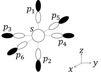
Figure 2: BO₆ cluster with the central $s$ orbital surrounded by six $p$ ligand orbitals. Note that for convenience, here we use a different convention for the signs of the $p_{1},p_{4}$ and $p_{6}$ orbitals than used in the lattice case depicted in Fig. 1.

The corresponding cluster model is:

$$\mathcal{H}= \Omega\sum^{6}_{i=1}b^{\dagger}_{i}b_{i}+\Delta s^{\dagger}s-\sum^{6}_{i=1}t(s^{\dagger}p_{i}+p_{i}^{\dagger}s)$$

$$-\sum^{6}_{i=1}\alpha t(s^{\dagger}p_{i}+p^{\dagger}_{i}s)(b^{\dagger}_{i}+b_{i})$$

$$-t_{p}\sum_{i=1,3,5}\left[(p^{\dagger}_{i}+p^{\dagger}_{i+1})(p_{i+2}+p_{i+3})+\text{h.c.}\right]$$

$$-\beta t_{p}\big{[}[p^{\dagger}_{6}(b^{\dagger}_{6}+b_{6})+p^{\dagger}_{5}(b^{\dagger}_{5}+b_{5})](p_{4}+p_{3})$$

$$+(p^{\dagger}_{5}+p^{\dagger}_{6})[p_{3}(b^{\dagger}_{3}+b_{3})+p_{4}(b^{\dagger}_{4}+b_{4})]+\dots\big{]}$$ (4)

where $i$ labels are cyclic with period 6. Note that we only listed explicitly a few of the terms in $H^{pp}$ (the last two lines). Writing all of them makes the equation too long, and is not illuminating. All the parameters have the same meaning as in Hamiltonian (1).

The cluster Hamiltonian can be written more simply in terms of hole and boson operators consistent with its symmetry. We define the new hole operators:

$$P_{1} =\frac{1}{\sqrt{6}}(p_{1}+p_{2}+\dots+p_{6})$$

$$P_{2} =\frac{1}{\sqrt{12}}(2p_{1}+2p_{2}-p_{3}-p_{4}-p_{5}-p_{6})$$

$$P_{3} =\frac{1}{\sqrt{4}}(p_{5}+p_{6}-p_{3}-p_{4})$$

$$P_{4} =\frac{1}{\sqrt{2}}(p_{6}-p_{5})$$

$$P_{5} =\frac{1}{\sqrt{2}}(p_{4}-p_{3})$$

$$P_{6} =\frac{1}{\sqrt{2}}(p_{1}-p_{2})$$

and similarly for the boson operators: $B_{1}=\sum_{i=1}^{6}b_{i}$, etc.

$P^{\dagger}_{1}$ creates a hole in the linear combination of O $2p$ orbitals with $A_{1g}$ ($s$-like) symmetry, $P^{\dagger}_{2}$ and $P^{\dagger}_{3}$ correspond to the $E_{g}$ terms with $d_{3z^{2}-r^{2}}$ and $d_{x^{2}-y^{2}}$ symmetry, respectively, and $P^{\dagger}_{4},P^{\dagger}_{5}$ and $P^{\dagger}_{6}$ correspond to the $T_{1u}$ terms with $p_{x}$, $p_{y}$ and $p_{z}$ symmetry, respectively. We define the new bosonic operators $B_{i}$ similarly.

In the new basis, the cluster Hamiltonian becomes:

$$\mathcal{H}=\Omega\sum_{i=1}^{6}B_{i}^{\dagger}B_{i}+\Delta s^{\dagger}s-T(s^{\dagger}P_{1}+P_{1}^{\dagger}s)$$

$$-\alpha t\sum^{6}_{i=1}(s^{\dagger}P_{i}+P_{i}^{\dagger}s)(B^{\dagger}_{i}+B_{i})$$

$$-t_{p}(4P_{1}^{\dagger}P_{1}-2P_{2}^{\dagger}P_{2}-2P_{3}^{\dagger}P_{3})$$

$$-\beta t_{p}\bigg{(}\sqrt{\frac{8}{3}}(B_{1}^{\dagger}+B_{1})(2P_{1}^{\dagger}P_{1}-P_{2}^{\dagger}P_{2}-P_{3}^{\dagger}P_{3})+\dots\bigg{)}$$ (5)

where the dots in the last line refer to terms involving phonon operators $B_{i}+B_{i}^{\dagger}$ with $i\neq 1$, i.e. the other $E_{g}$ and $T_{1u}$ symmetries are included. They are straightforward but too lengthy to write here. Note that because of the $pp$ hopping, the effective charge transfer energy between the $s$ and the $P_{1}$ molecular orbital is $\Delta_{1}=\Delta+4t_{p}$, whereas for the $E_{g}$ molecular orbitals, the effective charge transfer energy is $\Delta_{2}=\Delta_{3}=\Delta+2t_{p}$.

The third term shows that indeed, the $s$ orbital only hybridizes with the $P_{1}$ molecular orbital with the same $A_{1g}$ symmetry, and the effective hopping is $T=\sqrt{6}t$. However, because the presence of deformations breaks this symmetry, the Peierls $\alpha$ electron-phonon coupling allows hopping between the $s$ and any of the $P_{i}$ orbitals, if bosons with the same symmetry $i$ are either already present, or are being created during the process – see terms on the second line. Terms due to the $p$-$p$ hopping can be understood similarly.

III Methods

We studied the models described above by a variety of means which we briefly review here, with full details relegated to various appendixes.

III.1 Perturbation theory for the lattice case in the anti-adiabatic limit

In the antiadiabatic limit where $\Omega$ is the largest energy scale, we can use perturbation theory to project out the high-energy states with one or more phonons, to obtain an effective Hamiltonian describing the motion of the polaron. The resulting analytical dispersion is useful because it allows us to gain intuition about the behavior of the polaron in this limit, as discussed below.

We partition the Hamiltonian into $\hat{H}=\hat{h}_{0}+\hat{h}_{1}$, where $\hat{h}_{0}\equiv\Omega\sum_{i,\gamma}b^{\dagger}_{i\gamma}b_{i\gamma}$ is the large part, and $\hat{h}_{1}$ includes all the other terms and is treated as the perturbation. Using standard second order perturbation theory (PT),Takahashi (1977) we obtain the low-energy effective Hamiltonian to be:

$$\hat{h}=\hat{h}_{0}+\hat{P_{0}}\hat{h}_{1}\hat{P_{0}}+\hat{P_{0}}\hat{h}_{1}\frac{1-\hat{P_{0}}}{E_{0}-\hat{h}_{0}}\hat{h}_{1}\hat{P_{0}}+{\cal O}\left({1\over\Omega^{2}}\right)$$

where $\hat{P_{0}}$ is the projection operator onto the highly-degenerate, one-hole ground state manifold of $\hat{h}_{0}$, i.e. zero-phonon states with energy $E_{0}=0$.

After carrying out these calculations, we find that $\hat{h}=-\Delta\sum_{i\gamma}\gamma^{\dagger}_{i}\gamma_{i}+T_{sp}+T_{pp}+\delta\hat{h}+{\cal O}\left({1\over\Omega^{2}}\right)$ where:

$$\delta\hat{h}=-\frac{\alpha^{2}t^{2}}{\Omega}\sum_{j\gamma}(\tilde{s}^{\dagger}_{j,\gamma}+\tilde{s}^{\dagger}_{j-\gamma,\gamma})s_{j}-\frac{2\alpha^{2}t^{2}+8\beta^{2}t_{p}^{2}}{\Omega}\sum_{j\gamma}\gamma^{\dagger}_{j}\gamma_{j}$$

$$+\frac{\alpha\beta tt_{p}}{\Omega}\sum_{j\gamma}(\bar{\gamma}^{\dagger}_{j,\gamma^{\prime}}+\bar{\gamma}^{\dagger}_{j,\gamma^{\prime\prime}}+\bar{\gamma}^{\dagger}_{j-\gamma,\gamma^{\prime}}+\bar{\gamma}^{\dagger}_{j-\gamma,\gamma^{\prime\prime}})s_{j}\qquad$$

$$-\frac{\alpha\beta tt_{p}}{\Omega}\sum_{j\gamma}(-\tilde{s}^{\dagger}_{j,\gamma^{\prime\prime}}+\tilde{s}^{\dagger}_{j+\gamma,\gamma^{\prime\prime}}-\tilde{s}^{\dagger}_{j-\gamma^{\prime\prime},\gamma^{\prime\prime}}+\tilde{s}^{\dagger}_{j+\gamma-\gamma^{\prime\prime},\gamma^{\prime\prime}}$$

$$-\tilde{s}^{\dagger}_{j,\gamma^{\prime}}+\tilde{s}^{\dagger}_{j+\gamma,\gamma^{\prime}}-\tilde{s}^{\dagger}_{j-\gamma^{\prime},\gamma^{\prime}}+\tilde{s}^{\dagger}_{j+\gamma-\gamma^{\prime},\gamma^{\prime}})\gamma_{j}\qquad$$

$$-\frac{\beta^{2}t_{p}^{2}}{\Omega}\sum_{j\gamma}(\bar{\gamma}^{\prime\prime\dagger}_{j,\gamma}+\bar{\gamma}^{\prime\prime\dagger}_{j,\gamma^{\prime}}-\bar{\gamma}^{\prime\prime\dagger}_{j+\gamma,\gamma}-\bar{\gamma}^{\prime\prime\dagger}_{j+\gamma,\gamma^{\prime}}+\bar{\gamma}^{\prime\prime\dagger}_{j-\gamma^{\prime\prime},\gamma}\qquad$$

$$+\bar{\gamma}^{\prime\prime\dagger}_{j-\gamma^{\prime\prime},\gamma^{\prime}}-\bar{\gamma}^{\prime\prime\dagger}_{j+\gamma-\gamma^{\prime\prime},\gamma}-\bar{\gamma}^{\prime\prime\dagger}_{j+\gamma-\gamma^{\prime\prime},\gamma^{\prime}}+\bar{\gamma}^{\prime\dagger}_{j,\gamma^{\prime\prime}}\qquad$$

$$+\bar{\gamma}^{\prime\dagger}_{j,\gamma}-\bar{\gamma}^{\prime\dagger}_{j+\gamma,\gamma^{\prime\prime}}-\bar{\gamma}^{\prime\dagger}_{j+\gamma,\gamma}+\bar{\gamma}^{\prime\dagger}_{j-\gamma^{\prime},\gamma^{\prime\prime}}\qquad$$

$$+\bar{\gamma}^{\prime\dagger}_{j-\gamma^{\prime},\gamma}-\bar{\gamma}^{\prime\dagger}_{j+\gamma-\gamma^{\prime},\gamma^{\prime\prime}}-\bar{\gamma}^{\prime\dagger}_{j+\gamma-\gamma^{\prime},\gamma})\gamma_{j}\qquad$$ (6)

and we used the short-hand notation:

$$\tilde{s}^{\dagger}_{j,\gamma} \equiv s^{\dagger}_{j}+s^{\dagger}_{j+\gamma}$$

$$\bar{\gamma}^{\dagger}_{j,\gamma^{\prime}} \equiv\gamma^{\prime\dagger}_{j}-\gamma^{\prime\dagger}_{j-\gamma^{\prime}}+\gamma^{\prime\dagger}_{j+\gamma}-\gamma^{\prime\dagger}_{j+\gamma-\gamma^{\prime}}.$$

The expression of $\delta\hat{h}$ may seem complicated, but it consists of simple terms whose appearance is conceptually straightforward to understand. They can be divided into on-site energies like $-6\alpha^{2}t^{2}/\Omega\sum_{j}s^{\dagger}_{j}s_{j}$ (part of the first term on the first line), which reflect the polaron formation energy as a hole located at an $s$-site hops to a neighbor O and back while creating and then reabsorbing a phonon at that O site. The on-site energy at the O sites is also renormalized (last term on the first line) but by a different amount, so together these two terms imply a change of the efective $\Delta$.

All other terms describe longer-range hoping dynamically generated through phonon emission+absorption. For example, the first term on the first line contains terms proportional to $s^{\dagger}_{j^{\prime}}s_{j}$, where $j^{\prime}$ and $j$ are nn neighbor $s$ orbitals. These terms are generated when a hole hops from site $j$ to the O located in between $j$ and $j^{\prime}$ while creating a phonon at that O, and then hops again while absorbing the phonon, and lands at site $j^{\prime}$. Similar processes generate additional $s$-$p$ and $p$-$p$ hoppings, which supplement and renormalize the bare hopping $T_{sp}+T_{pp}$ and will therefore modify the polaron dispersion.

To find the polaron dispersion, we Fourier transform $\hat{h}$. For any $\bm{k}$-point in the cubic Brillouin zone, we get a $4\times 4$ matrix that can be diagonalized numerically. The lowest of the four bands is the polaron band.

III.2 Perturbation theory for the lattice case for weak electron-phonon coupling

Another case that can be treated with standard PT is when the electron-phonon coupling $\alpha\rightarrow 0$. For simplicity, we set $\beta=0$ and treat only the equivalent 1D caseMöller and Berciu (2016) – this suffices for our needs. The more general 3D case with $\beta\neq 0$ can be treated similarly.

Using Rayleigh-Schrödinger perturbation to second-order, the polaron energy is:

$$E_{P}(k)=E_{0}(k)+\frac{(\alpha t)^{2}}{8\pi}\int_{-\pi}^{\pi}dq\bigg{[} -(1+e^{-i(k-q)})(1+e^{ik})\left(\frac{1}{E_{0}(k)-\Omega-E_{0}(k-q)}-\frac{1}{E_{0}(k)-\Omega+E_{0}(k-q)}\right)$$

$$+(1+e^{-i(k-q)})(1+e^{i(k-q)})\left(\frac{1}{E_{0}(k)-\Omega-E_{0}(k-q)}+\frac{1}{E_{0}(k)-\Omega+E_{0}(k-q)}\right)$$

$$+(1+e^{ik})(1+e^{-ik})\left(\frac{1}{E_{0}(k)-\Omega-E_{0}(k+q)}+\frac{1}{E_{0}(k)-\Omega+E_{0}(k+q)}\right)$$

$$-(1+e^{-ik})(1+e^{i(k+q)})\left(\frac{1}{E_{0}(k)-\Omega-E_{0}(k+q)}-\frac{1}{E_{0}(k)-\Omega+E_{0}(k+q)}\right)\bigg{]}$$ (7)

where $E_{0}(k)=-|2t\sin(k/2)|$ is the free-hole dispersion and $a=1$. This result is only valid for phonon energy $\Omega>2|t|$, because otherwise the denominators vanish for large enough $k$ (Brillouin-Wigner PT must be used in this case). For $\alpha=0$, the GS is at $k=\pi$ and has energy $E_{0}(\pi)=-2|t|$, while $E_{0}(0)=0$. Note the additional phase-factors inside the integrand. These appear because the Peierls electron-phonon vertex, when Fourier transformed, depends explicitly on both the hole momentum $k$ and the phonon momentum $q$. This $(k,q)$ dependence is a direct consequence of the non-diagonal nature of the Peierls coupling, and is very unlike the Holstein model, where this vertex is a constant.

III.3 Momentum Average (MA) approximation for the lattice case

MA is a variational method for calculating the one-hole Green’s functions $G^{\beta\alpha}(\bf{k},\omega)\equiv\matrixelement{0}{\beta_{\bf{k}}\hat{G}(\omega)\alpha^{\dagger}_{\bf{k}}}{0}$, where $\alpha,\beta\in\{s,x,y,z\}$ are any pair of orbitals, $\hat{G}(\omega)=\left[\omega+i\eta-\hat{H}\right]^{-1}$ is the rezolvent for the Hamiltonian of Eq. (1), and $|\bm{0}\rangle$ is the vacuum for holes and phonons.

Here we present a brief overview of MA, with technical details relegated to Appendix A. To find $G^{\beta\alpha}(\bf{k},\omega)$, we use Dyson’s identity: $\hat{G}(\omega)=\hat{G_{0}}(\omega)+\hat{G}(\omega)\hat{V}\hat{G_{0}}(\omega)$, where $\hat{H_{0}}$ is the Hamiltonian of Eq. (2), $\hat{V}=\hat{H}-\hat{H_{0}}$, and $\hat{G_{0}}(\omega)=[\omega+i\eta-\hat{H_{0}}]^{-1}$ is the rezolvent for $\hat{H_{0}}$, whose corresponding propagators $G_{0}^{\beta\alpha}(\bf{k},\omega)=\matrixelement{0}{\beta_{\bf{k}}\hat{G_{0}}(\omega)\alpha^{\dagger}_{\bf{k}}}{0}$ can be calculated by Chebyshev Polynomials expansion, as explained in Appendix B. Using Dyson’s identity leads to the exact equation:

$$G^{\beta\alpha}({\bf{k}},\omega)= G^{\beta\alpha}_{0}({\bf{k}},\omega)-\alpha t\sum_{\gamma}(1+e^{i{\bf{k}}_{\gamma}a})\tilde{f}^{(1)}_{\gamma,\gamma}G^{s\alpha}_{0}({\bf{k}},\omega)$$

$$-\sum_{\gamma}[\alpha t\tilde{f}^{(1)}_{s,\gamma}-\beta t_{p}(\bar{f}^{(1)}_{\gamma^{\prime},\gamma}+\bar{f}^{(1)}_{\gamma^{\prime\prime},\gamma}+\xi_{\gamma^{\prime\prime}\gamma}({\bf{k}})\bar{f}^{(1)}_{\gamma^{\prime\prime},\gamma^{\prime\prime}}+\xi_{\gamma^{\prime}\gamma}({\bf{k}})\bar{f}^{(1)}_{\gamma^{\prime},\gamma^{\prime}})]G^{\gamma\alpha}_{0}({\bf{k}},\omega)$$ (8)

where we defined the generalized propagators

$$f^{(n)}_{\gamma,\delta,\ell}({\bf{k}},\omega)\equiv\sum_{j}\frac{e^{i{\bf{k}}R_{j}}}{N}\matrixelement{0}{\beta_{\bf{k}}\hat{G}(\omega)\gamma^{\dagger}_{j+\ell}(b^{\dagger}_{j\delta})^{n}}{0}$$ (9)

and we use the short-hand notations:

$$\xi_{\gamma_{1},\gamma_{2}}({\bf{k}})\equiv 1-e^{-i{\bf{k}}_{\gamma_{2}}a}+e^{i{\bf{k}}_{\gamma_{1}}a}-e^{i({\bf{k}}_{\gamma_{1}}-{\bf{k}}_{\gamma_{2}})a}$$

$$\tilde{f}^{(n)}_{s,\gamma}\equiv f^{(n)}_{s,\gamma,0}+f^{(n)}_{s,\gamma,\gamma}$$

$$\tilde{f}^{(n)}_{\gamma,\gamma}\equiv f^{(n)}_{\gamma,\gamma,0}$$

$$\bar{f}^{(n)}_{\gamma_{1},\gamma_{2}}\equiv f^{(n)}_{\gamma_{1},\gamma_{2},0}-f^{(n)}_{\gamma_{1},\gamma_{2},-\gamma_{1}}+f^{(n)}_{\gamma_{1},\gamma_{2},\gamma_{2}}-f^{(n)}_{\gamma_{1},\gamma_{2},\gamma_{2}-\gamma_{1}}$$

in which for simplicity, the dependence on $({\bf{k}},\omega)$ of the various $f$-propagators is not written explicitly.

To find equations of motion for the various $f^{(1)}$ propagators appearing in Eq. (III.3), we apply again Dyson’s identity. The electron-phonon coupling terms either remove the phonon, linking the various $f^{(1)}$ back to various $G^{\beta\alpha}({\bf{k}},\omega)$, or add a phonon and thus also link to new propagators with two phonons present in the initial (ket) state. If the two phonons are on the same O site, the corresponding propagator is one of the $f^{(2)}$ defined in Eq. (9) and we keep it, while we ignore the propagators with phonons located on different sites. The same procedure is employed to generate equations of motion for all $f^{(n)}$ for any $n\geq 2$, linking them to various $f^{(n-1)}$ and $f^{(n+1)}$.

The resulting equations, listed in Appendix (A) where we also discuss their solution, implement the variational guess that the largest weight to the polaron cloud comes from configurations where all phonons are at the same O site. That this should be a reasonable choice can be seen as follows: (i) if the hole is at an O site that is already displaced, i.e. it has phonons, the Peierls electron-phonon coupling $\alpha$ will hop it to one of its neighbor B sites and create an additional phonon at the original O site - this process is included in our variational calculation. The Peierls electron-phonon coupling $\beta$ will hope the hole to an adjacent O site, creating a new phonon either at the original O site (a process we include), or at the new O site (a process we ignore, because now there would be phonons on two different sites). Similarly, if (ii) the hole is at a B site neighbor to an O with several phonons, then a Peierls $\alpha$ process can take the hole back to the displaced O site, adding to the number of phonons there (we keep this), or to a different O site (we dismiss this as it would add a phonon at the new site). The reason is that each phonon costs an energy $\Omega$ but the hole cannot take advantage of (interact simultaneously with) phonons on multiple sites, so the most advantageous low-energy approach is to keep the phonon cloud spatially small.

We have tested this intuition for the 1D version of this model in Ref. Möller and Berciu, 2016, where we compared the MA results against those of exact diagonalization (ED) with excellent success. ED is prohibitively expensive in higher dimensions, but we know from extensive studies of MA for other models that its accuracy improves with increasing dimensionality Berciu (2006); Goodvin et al. (2006); Berciu and Goodvin (2007). Additionally, MA accuracy can be gauged by increasing the variational space. The simplest new configurations are those allowing an extra phonon on a different site than the one that already has a cloud. For the 2D version of this model we found that including these additional states has very small influence on the results, for instance changing eigenenergies by very few percent. Möller et al. (2017) We have not implemented the expanded variational calculation here because it becomes much more cumbersome in 3D and such small quantitative variations will not affect the conclusions we draw below.

III.4 Variational approximation for the cluster Hamiltonian

The spectrum of the cluster Hamiltonian of Eq. (5) can be found by exact diagonalization, but for our purposes it suffices to use a variational approximation that sets an upper bound to the ground-state energy. The best trial wavefunction we found is:

$$\ket{\psi_{v}}=\frac{s^{\dagger}+\sum_{i=1}^{6}\chi_{i}P_{i}^{\dagger}}{\sqrt{1+\sum_{i=1}^{6}\chi_{i}^{2}}}\prod_{i=1}^{6}e^{-\frac{1}{2}\eta_{i}^{2}+\eta_{i}B^{\dagger}_{i}}\ket{0}$$ (10)

where $\chi_{i}$ and $\eta_{i}$ are variational parameters defining the electronic part of the “cluster” orbital, and the coherent distortions associated with the various symmetries, respectively.

After some algebra, we find:

$$\matrixelement{\psi_{v}}{{\cal H}}{\psi_{v}}=\frac{\Delta-2t\chi_{1}}{1+\sum_{i}{\chi}_{i}^{2}}+\Omega\sum_{{}_{i}}\eta_{i}^{2}-\frac{4{\alpha t}\sum_{i}\chi_{i}\eta_{i}}{1+\sum_{i}{\chi}_{i}^{2}}+\dots$$

where the dots are terms coming from $p$-$p$ hopping, which we do not write here so as to keep the expression compact (however, these terms are included in the calculation). This is minimized numerically to find $\chi_{i}$ and $\eta_{i}$, which are then used to calculate an upper bound $\matrixelement{\psi_{v}}{{\cal H}}{\psi_{v}}$ for the cluster ground-state energy, which we will refer to as the “variational” cluster energy.

III.5 $A_{1g}$ approximation for the cluster Hamiltonian

Given that the $s$ orbital only hybridizes with the $P_{1}$ orbital with a large $T=\sqrt{6}t$, one may expect that the terms with $A_{1g}$ symmetry contribute most to the ground-state. This implies a symmetric, $s$-like distortion of the O cage. We could then remove from the cluster Hamiltonian the terms with boson operators of other symmetries, and still expect a good low-energy description.

The resulting simplified cluster Hamiltonian is:

$${\cal H}_{A_{1g}}= \Delta s^{\dagger}s+\Omega B_{1}^{\dagger}B_{1}-T(s^{\dagger}P_{1}+P_{1}^{\dagger}s)$$

$$-\alpha t(s^{\dagger}P_{1}+P_{1}^{\dagger}s)(B_{1}^{\dagger}+B_{1})$$

$$-4t_{p}P_{1}^{\dagger}P_{1}-4\sqrt{\frac{2}{3}}\beta t_{p}P_{1}^{\dagger}P_{1}(B_{1}^{\dagger}+B_{1})$$ (11)

We note again that the effective charge transfer energy is $\Delta_{1}=\Delta+4t_{p}$, however to make comparisons easier, we continue to work with the original parameters $\Delta$ and $t_{p}$.

The ground state energy for this Hamiltonian can be found using continued fractions, Berciu (2007) see also Appendix C. We will refer to it as the “$A_{1g}$” cluster energy.

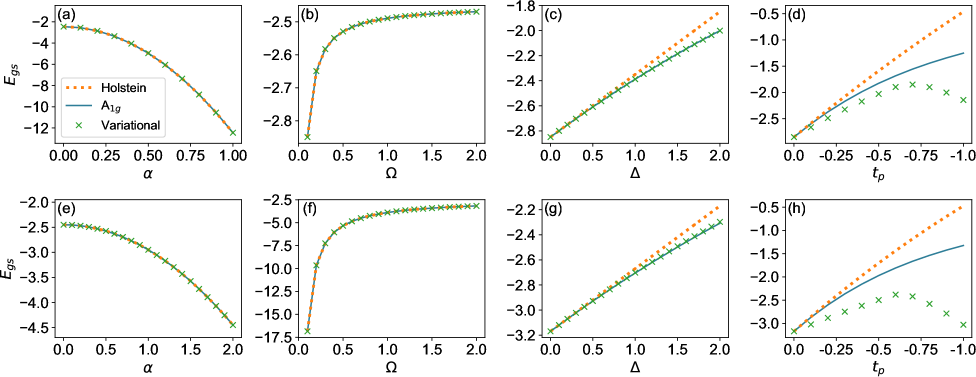
Figure 3: Comparison between the cluster ground state energies obtained with the variational (symbols), $A_{1g}$ (full line) and Holstein (dashed line) approximations, respectively, as a function of various parameters. If not otherwise specified, parameters used in (a)-(d) are $t=-1$, $t_{p}=0$, $\Delta=0$, $\Omega=0.1$ and $\alpha=0.2$; and in (e)-(h) $t=-1$, $t_{p}=0$, $\Delta=0$, $\Omega=2$ and $\alpha=1.2$. In all cases, $\beta=\frac{\alpha}{2}$.

III.6 Holstein approximation for the cluster Hamiltonian

We rewrite the electronic part of ${\cal H}_{A_{1g}}$ in terms of the (for holes) bonding $d_{1}^{\dagger}=(s^{\dagger}-P_{1}^{\dagger})/\sqrt{2}$ and anti-bonding $d_{2}^{\dagger}=(s^{\dagger}+P_{1}^{\dagger})/\sqrt{2}$ operators. For $T\gg\Delta$, the bonding orbital is located about $2T$ below the anti-bonding one, and we expect to get a good low-energy approximation by ignoring all terms involving $d_{2}$ operators.

The resulting simplified cluster Hamiltonian is:

$${\cal H}_{H}= \frac{\Delta}{2}d_{1}^{\dagger}d_{1}+\Omega B_{1}^{\dagger}B_{1}-Td_{1}^{\dagger}d_{1}+\alpha td_{1}^{\dagger}d_{1}(B_{1}^{\dagger}+B_{1})$$

$$\qquad-2\left[t_{p}+\sqrt{\frac{2}{3}}\beta t_{p}(B_{1}^{\dagger}+B_{1})\right]d_{1}^{\dagger}d_{1}$$

$$= \epsilon d_{1}^{\dagger}d_{1}+\Omega B_{1}^{\dagger}B_{1}+g_{H}d_{1}^{\dagger}d_{1}(B_{1}^{\dagger}+B_{1})$$

This defines a one-site Holstein model with effective parameters $\epsilon=\frac{\Delta}{2}-T-2t_{p}$ and $g_{H}=\alpha t-2\sqrt{\frac{2}{3}}\beta t_{p}$. It can be solved exactly, and has a one-hole ground-state energy $E_{H}=\epsilon-g_{H}^{2}/\Omega$. In the following, we refer to this as the “Holstein” cluster energy.

By comparing the variational, $A_{1g}$ and Holstein cluster energies, we can infer the validity of these various approximations in different regions of the parameter space, to see when/if a Holstein model provides a good low-energy description of the cluster. Together with the results for the lattice case, this will allow us to understand the equivalence (or lack theoreof) between the Peierls and the Holstein models on the perovskite lattice.

IV Results

In this section, the values chosen for the various parameters are for illustration purposes, so that a broad region of the parameter space can be sampled. Results specific to the values we believe to be appropriate for BaBiO₃ are presented and discussed in the last section.

IV.1 Results for the cluster

Figure 3 compares the cluster ground-state energies $E_{gs}$ obtained with the variational (symbols), $A_{1g}$ (full line) and Holstein (dashed line) approximations. In all cases, we use $|t|=1$ as the unit of energy. Panels (a) and (e) show the evolution of $E_{gs}$ with the Peierls coupling $\alpha$ (with $\beta=\alpha/2$ used throughout), when $t_{p}=0$ and $\Delta=0$. The phonon frequency is $\Omega=0.1$ in panel (a) and $\Omega=2$ in panel (e). The three approximations are in very good agreement. The same is true for panels (b) and (f), where we track the dependence of $E_{gs}$ on $\Omega$. Here, we continue to keep $t_{p}=\Delta=0$, and we set the Peierls coupling $\alpha=0.2$ in panel (b) and $\alpha=1.2$ in panel (f). We conclude that for vanishing $\Delta$ and $p$-$p$ hopping, a Holstein description is very satisfactory for the cluster for all phonon frequencies and electron-phonon couplings.

This is no longer the case, however, when either $\Delta\neq 0$ and/or $t_{p}\neq 0$. In panels (c) and (g) we track the dependence of $E_{gs}$ on $\Delta$, when $t_{p}=0$ and $\Omega=0.1,\alpha=0.2$ in panel (c), versus $\Omega=2,\alpha=1.2$ in panel (g). Both cases show good agreement between the variational and the $A_{1g}$ results, suggesting that the cluster distortion remains s-like. However, projecting out the anti-bonding orbital becomes increasingly inaccurate with increasing $\Delta$. This is because a large $\Delta$ favors a different mix between the $s$ and $P_{1}$ orbitals than the $50/50$ mix favored by the hybridization $T$ and by the electron-phonon coupling, see Eq. (11). As a result, there is no unique choice for a single “cluster” low-energy electronic orbital onto which to project, thus a Holstein-like description becomes increasingly inaccurate.

The problem is further exacerated if we add a finite $t_{p}$ hopping. This term is known to be important because it is primarily responsible for setting the bandwidth of the O band, which is generally considerable in perovskites. Physically, this is a consequence of the rather short distance between adjacent O, which means that $t_{p}$ is not negligible compared to $t$. As already noted, it also decreases the effective charge transfer energy between the $s$ and $P_{1}$ orbitals. The dependence of $E_{gs}$ on $|t_{p}|$ is shown in panels (d) and (h). In both cases $\Delta=0$, and the values of the other parameters are as in (c) and (g), respectively. For any finite $t_{p}$, the $A_{1g}$ approximation fails rather fast, and the Holstein one is even worse. The reason is that the $\beta$ Peierls coupling connects the $s$-like O distortion described by $B_{1},B_{1}^{\dagger}$ not just to the $P_{1}$ orbital with $A_{1g}$ symmetry, but also to the $E_{g}$ orbitals $P_{2},P_{3}$, see Eq. (5). In term, when the electron occupies one of these other orbitals, it favors the appearance of distortions with the same symmetry, see the $\alpha$ term in Eq. (5). The end result is that the other distortion modes are also activated, so now even the projection onto the $A_{1g}$ symmetry is inaccurate, making the further steps to a Holstein mapping impossible.

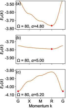
Figure 4: Polaron dispersion in the anti-adiabatic limit. These are perturbational results but in excellent agreement with the MA results. Parameters are $|t|=1,t_{p}=\Delta=0,\Omega=80$ and (a) $\alpha=4.8$, (b) $\alpha=5$, and (c) $\alpha=5.2$. Red dots indicate the ground-state.

Indeed, we find that the downturn of the variational energy at larger $t_{p}$ occurs because the $E_{g}$ symmetry starts to dominate over the $A_{1g}$ one, as shown by their weights in the variational calculation (not shown here). This is reminiscent of the phase transitionKhazraie et al. (2018b) in BaBiO₃ between the $A_{1g}$ dominated bond-disproportionated state and the $E_{g}$ metallic state, driven by the change of effective charge transfer energy $\Delta_{1}=\Delta+4t_{p}$.

It is important to emphasize that the activation of the cluster bosonic modes with other $E_{g}$ symmetries does not necessarily imply a non-symmetric distortion of the O cage (i.e. one breaking the cubic symmetry), so far as the average distortion is concerned. For example, activation of the $B_{3}$ ($x^{2}-y^{2}$) distortion will either bring the O on the $x$-bonds closer and push the $y$-bonds O further out, or viceversa. A wavefunction which has equal contributions from both positive and negative $B_{3}$ distortions will, in average, retain the cubic symmetry.

To conclude, the cluster results already demonstrate that an effective Holstein description is likely to fail for realistic systems with finite charge-transfer energies $\Delta\neq 0$ and finite $p$-$p$-hopping $t_{p}\neq 0$.

IV.2 Results for the lattice

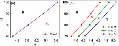
Figure 5: (a) Ground state momentum $\bm{k}_{gs}$ in the ($\Omega$, $\alpha$) parameter space, showing a sharp transition from $\bm{k}_{gs}=R$ to $\bm{k}_{gs}=G$. Here, $|t|=1,t_{p}=0,\Delta=0$. (b) same as in (a) but for $t_{p}=-0.2$. In this case, $\bm{k}_{gs}$ moves from $R\rightarrow M\rightarrow X\rightarrow G$.

As just shown, the cluster results indicate that the Holstein mapping is not valid in parts of the parameter space. We expect this conclusion to be even stronger for the lattice case, given its lower symmetry group.

To gain some intuition, we first use perturbation theory to study the evolution of the polaron dispersion in the anti-adiabatic limit $\Omega\gg t$. Of course, this limit is not physical, i.e. most materials are rather in the adiabatic limit (although this may change for “flat-band” materials). However, as we show below, the qualitative behaviour remains similar for all values of $\Omega$.

We first set $\Delta=0,t_{p}=0$ and study the evolution of the polaron dispersion with increasing $\alpha=4.8,5,5.2$ (and $\beta=\alpha/2$) for $\Omega=80$, $|t|=1$. The results are shown in Fig. 4. As customary, the high-symmetry points in the cubic Brillouin zone are $G=(0,0,0)$, $M=(\pi,\pi,0)$, $X=(\pi,0,0)$ and $R=(\pi,\pi,\pi)$ (we set $a=1$).

For a Holstein model, the polaron dispersion has roughly the same shape as the free-hole band, but its bandwidth decreases monotonically with increasing electron-phonon coupling. In contrast, here we see that for $\alpha>5$, the bandwidth starts to increase again. This is associated with a sharp switch of the momentum of the ground-state from $R$ to $G$, i.e. a change of the shape of the dispersion that is impossible for a Holstein model Gerlach and Löwen (1991). In Fig. 5(a) we show the location of this sharp transition in the $(\alpha,\Omega)$ plane, when $t_{p}=0,\Delta=0$ and $\Omega\gg 1$.

We now consider what happens when $\Delta\neq 0,t_{p}\neq 0$. We find that if $t_{p}=0$, setting $\Delta\neq 0$ simply shifts the location of the transition in the parameter space (not shown). More spectacular is the case $t_{p}\neq 0$, where as $\alpha$ increases, we find not one but three closely spaced ground-state transitions from $R\rightarrow M\rightarrow X\rightarrow G$, see Fig. 5(b). The evolution of the polaron dispersion across these transitions is shown in Fig. 6, again for an unphysical value $\Omega=80$.

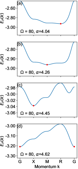
Figure 6: Evolution of the polaron dispersion with $\alpha$, when $t_{p}=-0.2$. Parameters not explicitly listed in the panels are as for Fig. 4.

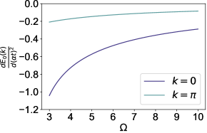
Figure 7: Measure of the polaron energy $E_{P}(k)$ on the coupling $\alpha$, in the limit $\alpha\rightarrow 0$. Note that for $k=0$, the polaron energy decreases faster with $\alpha$ than for $k=\pi$. These are 1D results obtained with weak-coupling PT of Eq. (7). Parameters are $t=-1,t_{p}=0,\Delta=0$.

Similar sharp transitions (sudden jumps) of the GS momentum between high-symmetry points have also been found for the 1D and 2D versions of this model, see Refs. Möller and Berciu, 2016; Möller et al., 2017. They can be understood in several ways.

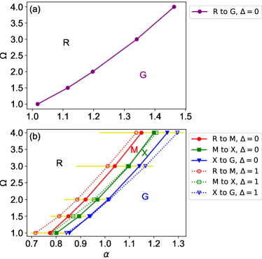
Figure 8: Ground state momentum transition in $(\alpha,\Omega)$ space, for smaller $\Omega$. Panel (a) is for $t_{p}=0,\Delta=0$, while panel (b) is for $t_{p}=-0.2,\Delta=0$ (straight lines) and $t_{p}=-0.2,\Delta=1$ (dotted lines). Yellow markers show typical size of errors in locating transitions. In the MA calculations for these graphs, $50^{3}$ unit cells are used for the 3D lattice and 300 terms are summed in the Chebyshev expansions for the free-hole propagators $G_{0}^{\alpha\beta}({\bf{k}},\omega)$. Other parameters are $t=-1$ and $\eta=0.1$.

In the anti-adiabatic limit, PT shows that the main effect of the Peierls electron-phonon coupling is to dynamically generate longer-range hopping terms and to renormalize the charge-transfer energy, see $\delta\hat{h}$ of Eq. (6) and following discussion. These longer-range hoppings favor a different $\bm{k}_{gs}$ than that of the bare-hole dispersion, and thus the transition occurs when the electron-phonon coupling is strong enough that these new terms dominate the polaron dispersion. For $t_{p}\neq 0$, the number of such phonon-mediated longer-range hoppings increases further and the resulting, more complex polaron dispersion, has more transitions. More discussion along these lines is available in Ref. Möller and Berciu, 2016.

This argument, however, is predicated on the system being in the anti-adiabatic limit, and thus one might wonder if similar physics is seen at lower, more physical values of $\Omega$. Before showing results proving that this is indeed the case, we first provide a second argument explaining the origin of the $\bm{k}_{gs}$ jump(s). This is based on PT for weak electron-phonon coupling. For simplicity, we carry out this analysis for the 1D equivalent of our 3D model.

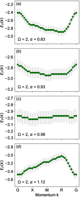
Figure 9: Polaron dispersion calculated with MA for $t=-1,\Omega=2,t_{p}=-0.2,\Delta=0$ and $\alpha$ values as indicate on the panels. For small $\alpha$ we find $\bm{k}_{gs}=R$, see panel (a), while for large $\alpha$ we find $\bm{k}_{gs}=G$. At intermediary values, the GS is also found at M and X.

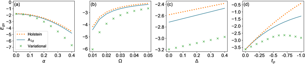
Figure 10: Comparison between the cluster ground state energies using parameters of BaBiO₃ obtained with the variational (symbols), $A_{1g}$ (full line) and Holstein (dashed line) approximations, respectively, as a function of various parameters. If not otherwise specified, parameters used in (a)-(d) are the BaBiO₃ parameters in units of $|t|=2.10$, namely $t=-1$, $t_{p}=-0.3$, $\Delta=0.19$, $\Omega=0.033$ and $\alpha=0.206$.

As shown in Eq. (7), the PT expression for $E_{P}(k)$ depends on $k$ not just through the usual energy denominators, but also because of the explicit $(k,q)$ dependence of the Peierls electron-phonon vertex. The latter essentially means that holes with different momenta $k$ couple with different strengths to the phonons, and this will affect how fast their energy is lowered with increasing $\alpha$. Indeed, in Fig. 7 we plot $dE_{P}(k)/d(\alpha t)^{2}$ when $\alpha\rightarrow 0$, as a measure of this dependence of $E_{P}(k)$ on $\alpha$. Both at $k=0$ and at $k=\pi$ the values are negative, as expected, showing a lowering of the energy in the presence of electron-phonon coupling. However, the slopes are very different, with $E_{P}(0)$ moving faster towards lower-energies than $E_{P}(\pi)$. This explains how it is possible that at a large enough $\alpha$, the GS momentum will switch from the free-hole value $k_{gs}=\pi$ to $k_{gs}=0$, instead. Also note that this difference is enhanced as one moves towards the adiabatic limit, suggesting that the existence of the transition(s) should be expected for any $\Omega$, not just in the anti-adiabatic limit. We confirm this below.

The existence of these sharp transitions of the ground-state of the Peierls model shows that it cannot be universally mapped onto a simpler Holstein model, because the ground-state of the latter cannot exhibit sharp transitions, instead its ground-state momentum is pinned at the free-hole value. Interestingly, the transition appears even for $t_{p}=0,\Delta=0$, see Fig. 5(a), so even here the mapping of Peierls onto Holstein does not work for the lattice case, even though the single cluster is modelled well by a Holstein Hamiltonian. This is proof of the fact that adequate cluster mapping is a necessary but not a sufficient condition for adequate lattice mapping.

Finally, we use MA to show that qualitatively similar behavior is seen at lower, more physical values of $\Omega$. Indeed, we find that the sharp transitions persist, specifically again if $t_{p}=0$ there is one from $R\rightarrow{G}$, see Fig. 8(a), and if $t_{p}\neq 0$ there are three from $R\rightarrow M\rightarrow X\rightarrow G$, see Fig. 8(b). In panel (b) we also show the slight shift of these transition lines if we set $\Delta=1$. Note the rather large error bars in the location of these transitions, shown in Fig. 8(b). Their origin is the difficulty to accurately calculate the free-hole propagators $G_{0}^{\alpha\beta}({\bf{k}},\omega)$. In order to smooth out fast oscillations in their $\omega$-dependence – the finite cutoff in the Chebyshev polynomials expansion means that we are effectively considering a finite size lattice, thus discretizing the free-hole spectrum – we are forced to use a rather large value $\eta=0.1$. This sets a limit for our accuracy in identifying the polaron energy, also see Fig. 9, which then translates into the uncertainty in figuring out when the ground-state momentum jumps from one high-symmetry point, to another. However, the shape and evolution of the spectra are consistent with what we found in the antiadiabatic limit thus giving us confidence that these transitions do occur, in other words that the ground-state momentum switches from R to G as the strength of the electron-phonon coupling is increased.

V Discussion

We used the MA approximation as well as various perturbative limits to study single polaron physics on a perovskite lattice inspired by BaBiO₃. The main motivation was to study a multi-band model with Peierls-type of electron-phonon coupling, whereby the motion of ions modulates the value of the hopping integrals between sites, to see if it can be mapped onto a much simpler one-band, Holstein model.

We find clear evidence of sharp transitions in the polaron ground-state properties, something that is proved to be impossible for a Holstein modelGerlach and Löwen (1991) (more generally, for any $g(q)$ models including the Rice-Sneddon model). This clearly demonstrates that when considered over the entire parameters space, it is impossible to capture the polaronic physics of the Peierls model with a much simpler Holstein model. The latter is inaccurate not just quantitatively, but qualitatively. Moreover, we showed that it is not enough to study a small cluster to decide this matter, instead one truly needs to study a lattice case. This is because the cluster solution suggested that mapping onto a Holstein model is good when $\Delta=t_{p}=0$, whereas the lattice results demonstrate that even in this case, a sharp transition occurs with increased electron-phonon coupling.

Thus, our main conclusion is that serious care is needed in deciding which model to use to describe the electron-phonon coupling in complicated structures such as the perovskites, one should not assume that such details do not matter and that the simplest option is safe.

This being said, we re-emphasize the fact that this conclusion is valid in the insulating limit, where there is a single carrier in the system so that a single polaron forms - this limit can be studied with the well-established MA approximation, supplemented and reinforced with PT results. Unfortunately, at this time we do not have access to similarly accurate approximations that deal with finite concentrations of carriers, so we cannot make any confident claims about such systems. The same is true even for the single polaron in the strongly adiabatic limit, where we know that the variational space used for the MA implemented here is too limited. These questions remain to be studied in future work.

Keeping in mind the caveats mentioned above, we now apply these methods to consider BaBiO₃. We use $t=-1$, $t_{p}=-0.3$, $\Delta=0.19$, $\Omega=0.033$ and $\alpha=0.206$ as reasonable parameters, following the work of Ref. Khazraie et al., 2018a. A very rough extrapolation of the curves shown in Fig. 8(b) suggests that this point falls to the left of the transition lines (the GS momentum is still at $R$ like for the free carriers) although probably not by a lot.

This is confirmed if we consider the cluster results, shown in Fig. 10. Each panel has all but one of the parameters fixed at the above-mentioned values, while the varying parameter explores a range around the nominal BaBiO₃ value. In all cases we see discrepancies between the solution for the full cluster Hamiltonian (even when studied variationally) and the Holstein projection. In particular, panel (d) shows that $t_{p}=-0.3$ falls indeed to the left of the downturn where the $E_{g}$ modes start to dominate, in other words the $A_{1g}$ is still the important symmetry here, but not by much.

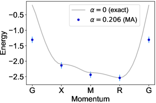
Figure 11: Dispersion for the 3D lattice Peierls model with parameters of BaBiO₃. Blue symbols with error bars show the MA results at the high symmetry points, for a system with 101³ sites and $\eta=0.1$. For comparison, the dispersion without electron phonon coupling (i.e. $\alpha=0$) was shown by the gray line, which was solved exactly algebraically.

For completeness, in Fig. 11 we also show MA results for the polaron dispersion corresponding to these parameters. Given the very low $\Omega/t$ ratio and the large $\eta$ used ($\eta=0.1$), we do not expect these results to be quantitatively very accurate, however they provide an upper bound on the actual polaron dispersion, because MA is a variational method. The main point is that the GS is still at the $R$ point, i.e. it is possible that this dispersion could be captured with an appropriately chosen Holstein model. Again, to what extent these conclusions hold for the finite hole concentrations that are physically relevant for BaBiO₃, is a matter for future studies.

Appendix A Details of the MA implementation

As discussed in the main text, we implement the simplest MA⁽⁰⁾ version, which allows phonon to appear only at one site in any given configuration. With this restriction, for $\gamma=s,x,y,z$ and $\delta=x,y,z$, we find that

$$f^{(n)}_{\gamma,\delta,\ell}= (\tilde{f}^{(n+1)}_{\delta,\delta}+n\tilde{f}^{(n-1)}_{\delta,\delta})[(-\alpha t)(G^{s\gamma}_{0,-\ell}+G^{s\gamma}_{0,-\ell+\delta})$$

$$+\beta t_{p}(\bar{g}^{\delta^{\prime}\gamma}_{-\ell}+\bar{g}^{\delta^{\prime\prime}\gamma}_{-\ell})]$$

$$+G^{\delta\gamma}_{0,-\ell}[(-\alpha t)(\tilde{f}^{(n+1)}_{s,\delta}+n\tilde{f}^{(n-1)}_{s,\delta})$$

$$+\beta t_{p}(\bar{f}^{(n+1)}_{\delta^{\prime},\delta}+\bar{f}^{(n+1)}_{\delta^{\prime\prime},\delta}+n\bar{f}^{(n-1)}_{\delta^{\prime},\delta}+n\bar{f}^{(n-1)}_{\delta^{\prime\prime},\delta})]$$

where $f\equiv f(\omega)$ while $G_{0}\equiv G_{0}(\omega-n\Omega)$ because of the cost of the $n$ phonons present, and then indexes $\gamma^{\prime},\gamma^{\prime\prime}$ associated with a given $\gamma$ are defined in the main text following Eq. (3). The free carrier propagators $G_{0}(\omega)$ are defined as:

$$\left\{\begin{array}[]{rll}G^{\gamma\gamma^{\prime}}_{0,i-j}(\omega)\equiv&\matrixelement{\gamma_{i}}{\hat{G_{0}}(\omega)}{\gamma^{\prime}_{j}}\\ \bar{g}^{\delta^{\prime}\gamma}_{-\ell}(\omega)\equiv&G^{\delta^{\prime}\gamma}_{0,-\ell}(\omega)-G^{\delta^{\prime}\gamma}_{0,-\ell-\delta^{\prime}}(\omega)+G^{\delta^{\prime}\gamma}_{0,-\ell+\delta}(\omega)\\ &-G^{\delta^{\prime}\gamma}_{0,-\ell+\delta-\delta^{\prime}}(\omega)\\ \bar{g}^{\delta^{\prime\prime}\gamma}_{-\ell}(\omega)\equiv&G^{\delta^{\prime\prime}\gamma}_{0,-\ell}(\omega)-G^{\delta^{\prime\prime}\gamma}_{0,-\ell-\delta^{\prime\prime}}(\omega)+G^{\delta^{\prime\prime}\gamma}_{0,-\ell+\delta}(\omega)\\ &-G^{\delta^{\prime\prime}\gamma}_{0,-\ell+\delta-\delta^{\prime\prime}}(\omega)\end{array}\right.$$

where $i$,$j$,$\ell$ are site indices.

Substituting these equations of motion for $f^{(n)}_{\gamma,\delta,\ell}$ into the definitions of $\tilde{f}^{(n)}_{s,\gamma}$, $\tilde{f}^{(n)}_{\gamma,\gamma}$, $\bar{f}^{(n)}_{\gamma^{\prime},\gamma}$ and $\bar{f}^{(n)}_{\gamma^{\prime\prime},\gamma}$, we find that the latter define recurrence relations linking propagators with a given $n$ only to those with $(n+1)$ and $(n-1)$. In other words, we can define a vector

$$v_{\gamma,n}^{T}\equiv\left(\tilde{f}^{(n)}_{s,\gamma},\tilde{f}^{(n)}_{\gamma,\gamma},\bar{f}^{(n)}_{\gamma^{\prime},\gamma},\bar{f}^{(n)}_{\gamma^{\prime\prime},\gamma}\right)^{T}$$

such that the equations of motion can be written in compact form as:

$$v_{\gamma,n}=\alpha_{\gamma n}v_{\gamma,n+1}+n\alpha_{\gamma n}v_{\gamma,n-1}$$

Here $\alpha_{\gamma n}$ is a known matrix whose entries can be read directly from the equations of motion. Note that for $n=0$, after some simplifications, $v_{\gamma,0}$ can be written in terms of the various propagators $G^{\alpha\beta}(\omega)$ of interest, specifically:

$$v_{\gamma,0} =\begin{bmatrix}(1+e^{-ik_{\gamma}a})G^{\beta s}(\omega)\\ G^{\beta\gamma}(\omega)\\ (1-e^{ik_{\gamma^{\prime}}a}+e^{-ik_{\gamma}a}-e^{i(k_{\gamma^{\prime}}-k_{\gamma})a})G^{\beta\gamma^{\prime}}(\omega)\\ (1-e^{ik_{\gamma^{\prime\prime}}a}+e^{-ik_{\gamma}a}-e^{i(k_{\gamma^{\prime\prime}}-k_{\gamma})a})G^{\beta\gamma^{\prime\prime}}(\omega)\end{bmatrix}$$

where $P_{\gamma}$ is a matrix and $\tilde{v_{0}}$ is defined to be $(G^{\beta s},G^{\beta x},G^{\beta y},G^{\beta z})^{T}$.

Such matrix recurrence relations are solved with the ansatz $v_{\gamma,n}=A_{\gamma,n}v_{\gamma,n-1}$ which allows us to calculate the matrices $A_{\gamma,n}$ recursively, starting from $A_{\gamma,N}=0$ for a sufficiently large $N$. This $N$ defines the largest number of phonons allowed to appear in a self-energy diagram, and is increased until the results converge. Once $A_{\gamma,n=1}$ is known, the various propagators $G^{\alpha\beta}(\omega)$ are obtained from Eq. (8).

Peaks in the spectral weights $-\frac{1}{\pi}\imaginary G^{\alpha\beta}(\omega)$ indicate the eigenenergies of $\hat{H}$, and thus allow us to determine the lowest eigenenergy for any given momentum $k$.

Appendix B Chebyshev Polynomial Expansion for Free Propagators

Such expansions are well established for a variety of problems. Here we briefly summarize the main steps, following Ref. Ferreira and Mucciolo, 2015.

Chebyshev polynomials $T_{n}(x)\equiv\cos(n\cos^{-1}(x))$ are well defined only for $x\in[-1,1]$, thus we need to rescale the range of eigenvalues of the non-interacting Hamiltonian $H_{0}$ before applying the Chebyshev expansion to it. $E_{max}$ and $E_{min}$ can be found by Fourier transforming $H_{0}$ to momentum $k$ space and maximizing or minimizing the energies in the $k$ parameter space. We define $a=\frac{E_{max}-E_{min}}{2}$ and $b=\frac{E_{max}+E_{min}}{2}$, and write the normalized Hamiltonian as $\tilde{H_{0}}=\frac{H_{0}-b}{a}$ and denote the corresponding non-interacting Green’s function as $\tilde{G_{0}}(\tilde{\omega})$, where $\tilde{\omega}$ is the scaled energy.

We expand Ferreira and Mucciolo (2015)

$$\tilde{G}^{\alpha\beta}_{0,j}(\tilde{\omega})=\sum^{\infty}_{n=0}2i^{-1}\frac{(\tilde{\omega}-i\sqrt{1-\tilde{\omega}^{2}})^{n}}{\sqrt{1-\tilde{\omega}^{2}}}\frac{\matrixelement{\alpha_{j}}{T_{n}(\tilde{H_{0}})}{\beta_{0}}}{1+\delta_{n0}}$$

where $T_{0}(x)=1$, $T_{1}(x)=x$ and $T_{n+1}(x)=2xT_{n}(x)-T_{n-1}(x)$.

If we define $\ket{J_{n}}\equiv T_{n}(\tilde{H_{0}})\ket{\beta_{0}}$, then $\ket{J_{n+1}}=2\tilde{H_{0}}\ket{J_{n}}-\ket{J_{n-1}}$, thus these $\ket{J_{n}}$ can be determined recursively starting from $\ket{J_{0}}=\ket{\beta_{0}}$ and $\ket{J_{1}}=\tilde{H_{0}}\ket{\beta_{0}}$. The summation is truncated at a value large enough so that $\tilde{G}^{\alpha,\beta}_{0,j}$ is converged. We note here that there are unphysical oscillations in the $\tilde{G}^{\alpha,\beta}_{0,j}$ obtained if plotted versus energy. This is caused by the standing waves selected due to the finite size of the system. Since $\eta$ is inversely proportional to the lifetime of the state, we can either increase the size of the system or use a larger $\eta$ so that the state cannot live long enough to reach the edge of the system, and hence the finite-size oscillations are smoothed out. Having a larger system would increase the demand for computational power exponentially, therefore we are forced to use a fairly large $\eta$ (0.1 in our case) in order to get a smooth enough curve for $\tilde{G}^{\alpha,\beta}_{0,j}$.

Rescaling back, the various free propagators are: $G^{\alpha\beta}_{0,j}(\omega+i\eta)=\frac{1}{a}\tilde{G}_{0,j}^{\alpha\beta}\bigg{(}\frac{\omega-b}{a}+i\frac{\eta}{a}\bigg{)}$.

Appendix C Details of the continued fraction solution for the cluster

We consider the Hamiltonian of Eq. (11), where two different electronic orbitals $s$ and $P_{1}$ (renamed $p$ in the following, for simplicity) are coupled to the same boson mode $B_{1}$ (renamed $b$ in the following, for simplicity). The full Hilbert space corresponding to the one-carrier sector is spanned by the basis $\{|s,n\rangle\equiv\frac{s^{\dagger}(b^{\dagger})^{n}\ket{0}}{\sqrt{n!}},|p,n\rangle\equiv\frac{p^{\dagger}(b^{\dagger})^{n}\ket{0}}{\sqrt{n!}}\}$ with $n\geqslant 0$.

We define the propagators:

$$\left\{\begin{array}[]{rcl}\mathcal{S}_{n}(m,z)&\equiv\langle s,n|\hat{G}(z)|s,m\rangle\\ \mathcal{P}_{n}(m,z)&\equiv\langle s,n|\hat{G}(z)|p,m\rangle\end{array}\right.$$

Their equations of motion are generated from the appropriate expectation values of the identity $\hat{G}(z)(z-\hat{H})=1$. For the Hamiltonian of Eq. (11), we find:

$$\mathcal{S}_{n}(m,z)(z-\Delta-m\Omega)+\mathcal{P}_{n}(m,z)t$$

$$-\mathcal{P}_{n}(m+1,z)\alpha t\sqrt{m+1}-\mathcal{P}_{n}(m-1,z)\alpha t\sqrt{m}=\delta_{mn}$$

and

$$\mathcal{S}_{n}(m,z)t-\mathcal{S}_{n}(m+1,z)\alpha t\sqrt{m+1}$$

$$-\mathcal{S}_{n}(m-1,z)\alpha t\sqrt{m}+\mathcal{P}_{n}(m,z)(z-\Omega m)=0$$

These can be grouped as recurrence equations for $2\times 2$ matrices:

$$\gamma_{m}W_{nm}-\alpha_{m}W_{n,m+1}-\beta_{m}W_{n,m-1}=\begin{bmatrix}\delta_{n,m}\\ 0\end{bmatrix}\quad\text{and}$$

where

$$\gamma_{m}\equiv\left[\begin{array}[]{cc}z-\Delta-m\Omega&t\\ t&z-\Omega m\end{array}\right];$$

$$\alpha_{m}\equiv\left[\begin{array}[]{cc}0&\alpha t\sqrt{m+1}\\ \alpha t\sqrt{m+1}&0\end{array}\right];\quad$$

$$\beta_{m}\equiv\left[\begin{array}[]{cc}0&\alpha t\sqrt{m}\\ \alpha t\sqrt{m}&0\end{array}\right];$$

$$W_{n,m}\equiv\begin{bmatrix}\mathcal{S}_{n}(m,z)\\ \mathcal{P}_{n}(m,z)\end{bmatrix}$$

As already discussed, such recurrence relations are solved with the ansatz $W_{n,m+1}=A_{n,m+1}W_{nm}$ if $m\geq n$. This gives the continued fraction $A_{nm}=(\gamma_{m}-\alpha_{m}A_{n,m+1})^{-1}\beta_{m}$, which can be evaluated starting from $A_{nM}=0$ for a sufficiently large $M$. Similarly, for $m\leq n$ we use the ansatz $W_{n,m-1}=B_{n,m-1}W_{n,m}$ and obtain $B_{n,m}=(\gamma_{m}-\beta_{m}B_{n,m-1})^{-1}\alpha_{m}$, which can be computed starting from $m=0$, noting that $\beta_{0}\equiv 0$.

Putting $W_{n,n+1}=A_{n,n+1}W_{nn}$ and $W_{n,n-1}=B_{n,n-1}W_{n,n}$ into the equation with $n=m$, we get:

$$W_{nn}=(\gamma_{n}-\alpha_{n}A_{n,n+1}-\beta_{n}B_{n,n-1})^{-1}\begin{bmatrix}1\\ 0\end{bmatrix}$$

from which we can read out the propagators $\mathcal{S}_{n}(m,z)$ and $\mathcal{P}_{n}(m,z)$.

References

- Gao et al. (1994) L. Gao, Y. Y. Xue, F. Chen, Q. Xiong, R. L. Meng, D. Ramirez, C. W. Chu, J. H. Eggert, and H. K. Mao, Phys. Rev. B 50, 4260 (1994).
- Presland et al. (1991) M. Presland, J. Tallon, R. Buckley, R. Liu, and N. Flower, Physica C: Superconductivity 176, 95 (1991).
- Tallon et al. (1995) J. L. Tallon, C. Bernhard, H. Shaked, R. L. Hitterman, and J. D. Jorgensen, Phys. Rev. B 51, 12911 (1995).
- Obertelli et al. (1992) S. D. Obertelli, J. R. Cooper, and J. L. Tallon, Phys. Rev. B 46, 14928 (1992).
- Subedi et al. (2015) A. Subedi, O. E. Peil, and A. Georges, Phys. Rev. B 91, 075128 (2015).
- Srivastava et al. (2009) C. M. Srivastava, N. B. Srivastava, L. N. Singh, and D. Bahadur, Journal of Applied Physics 105, 093908 (2009).
- Abdelkhalek et al. (2011) S. B. Abdelkhalek, N. Kallel, S. Kallel, T. Guizouarn, O. Peña, and M. Oumezzine, Physica B: Condensed Matter 406, 4060 (2011).
- Liu and Yang (2017) H. Liu and X. Yang, Ferroelectrics 507, 69 (2017).
- Anderson (1987) P. W. Anderson, Science 235, 1196 (1987).
- Emery (1987) V. J. Emery, Phys. Rev. Lett. 58, 2794 (1987).
- Jiang et al. (2020) M. Jiang, M. Moeller, M. Berciu, and G. A. Sawatzky, Phys. Rev. B 101, 035151 (2020).
- Johnston et al. (2014) S. Johnston, A. Mukherjee, I. Elfimov, M. Berciu, and G. A. Sawatzky, Phys. Rev. Lett. 112, 106404 (2014).
- Park et al. (2012) H. Park, A. J. Millis, and C. A. Marianetti, Phys. Rev. Lett. 109, 156402 (2012).
- Pankaj and Yarlagadda (2012) R. Pankaj and S. Yarlagadda, Phys. Rev. B 86, 035453 (2012).
- Kurdestany and Satpathy (2017) J. M. Kurdestany and S. Satpathy, Phys. Rev. B 96, 085132 (2017).
- Holstein (1959) T. Holstein, Annals of Physics 8, 325 (1959).
- Fröhlich et al. (1950) H. Fröhlich, H. Pelzer, and S. Zienau, The London, Edinburgh, and Dublin Philosophical Magazine and Journal of Science 41, 221 (1950).
- Kurzynski (1976) M. Kurzynski, Journal of Physics C: Solid State Physics 9, 3731 (1976).
- Lau et al. (2007) B. Lau, M. Berciu, and G. A. Sawatzky, Phys. Rev. B 76, 174305 (2007).
- Goodvin and Berciu (2008) G. L. Goodvin and M. Berciu, Phys. Rev. B 78, 235120 (2008).
- Alexandrov (2008) A. S. Alexandrov, Polarons in advanced materials, Vol. 103 (Springer Science & Business Media, 2008).
- Savrasov and Andersen (1996) S. Y. Savrasov and O. K. Andersen, Phys. Rev. Lett. 77, 4430 (1996).
- Zhang and Rice (1988) F. C. Zhang and T. M. Rice, Phys. Rev. B 37, 3759 (1988).
- Yin et al. (2008) Q. Yin, A. Gordienko, X. Wan, and S. Y. Savrasov, Phys. Rev. Lett. 100, 066406 (2008).
- Khaliullin and Horsch (1997) G. Khaliullin and P. Horsch, Physica C: Superconductivity 282-287, 1751 (1997).
- Shen et al. (2004) K. M. Shen, F. Ronning, D. H. Lu, W. S. Lee, N. J. C. Ingle, W. Meevasana, F. Baumberger, A. Damascelli, N. P. Armitage, L. L. Miller, Y. Kohsaka, M. Azuma, M. Takano, H. Takagi, and Z.-X. Shen, Phys. Rev. Lett. 93, 267002 (2004).
- Goodvin (2009) G. L. Goodvin, Ph.D. thesis, University of British Columbia (2009).
- Hamada et al. (1989) N. Hamada, S. Massidda, A. J. Freeman, and J. Redinger, Phys. Rev. B 40, 4442 (1989).
- Shirai et al. (1990) M. Shirai, N. Suzuki, and K. Motizuki, Journal of Physics: Condensed Matter 2, 3553 (1990).
- Liechtenstein et al. (1991) A. I. Liechtenstein, I. I. Mazin, C. O. Rodriguez, O. Jepsen, O. K. Andersen, and M. Methfessel, Phys. Rev. B 44, 5388 (1991).
- Kunc and Zeyher (1994) K. Kunc and R. Zeyher, Phys. Rev. B 49, 12216 (1994).
- Meregalli and Savrasov (1998) V. Meregalli and S. Y. Savrasov, Phys. Rev. B 57, 14453 (1998).
- Bazhirov et al. (2013) T. Bazhirov, S. Coh, S. G. Louie, and M. L. Cohen, Phys. Rev. B 88, 224509 (2013).
- Khazraie et al. (2018a) A. Khazraie, K. Foyevtsova, I. Elfimov, and G. A. Sawatzky, Phys. Rev. B 97, 075103 (2018a).
- Kostur and Allen (1997) V. N. Kostur and P. B. Allen, Phys. Rev. B 56, 3105 (1997).
- Allen and Kostur (1997) P. B. Allen and V. N. Kostur, Zeitschrift für Physik B Condensed Matter 104, 613 (1997).
- Piekarz and Konior (2000) P. Piekarz and J. Konior, Physica C: Superconductivity 329, 121 (2000).
- Bischofs et al. (2002) I. B. Bischofs, V. N. Kostur, and P. B. Allen, Phys. Rev. B 65, 115112 (2002).
- Nourafkan et al. (2012) R. Nourafkan, F. Marsiglio, and G. Kotliar, Phys. Rev. Lett. 109, 017001 (2012).
- Seibold and Sigmund (1993) G. Seibold and E. Sigmund, Solid State Communications 86, 517 (1993).
- Gerlach and Löwen (1991) B. Gerlach and H. Löwen, Rev. Mod. Phys. 63, 63 (1991).
- Harrison (2004) W. Harrison, Elementary Electronic Structure (World Scientific, 2004).
- Foyevtsova et al. (2015) K. Foyevtsova, A. Khazraie, I. Elfimov, and G. A. Sawatzky, Phys. Rev. B 91, 121114 (2015).
- Takahashi (1977) M. Takahashi, Journal of Physics C: Solid State Physics 10, 1289 (1977).
- Möller and Berciu (2016) M. M. Möller and M. Berciu, Phys. Rev. B 93, 035130 (2016).
- Berciu (2006) M. Berciu, Phys. Rev. Lett. 97, 036402 (2006).
- Goodvin et al. (2006) G. L. Goodvin, M. Berciu, and G. A. Sawatzky, Phys. Rev. B 74, 245104 (2006).
- Berciu and Goodvin (2007) M. Berciu and G. L. Goodvin, Phys. Rev. B 76, 165109 (2007).
- Möller et al. (2017) M. M. Möller, G. A. Sawatzky, M. Franz, and M. Berciu, Nature Communications 8, 2267 (2017).
- Berciu (2007) M. Berciu, Phys. Rev. B 75, 081101 (2007).
- Khazraie et al. (2018b) A. Khazraie, K. Foyevtsova, I. Elfimov, and G. A. Sawatzky, Phys. Rev. B 98, 205104 (2018b).
- Ferreira and Mucciolo (2015) A. Ferreira and E. R. Mucciolo, Phys. Rev. Lett. 115, 106601 (2015).