Quadrilateral Mesh Generation III : Optimizing Singularity Configuration Based on Abel-Jacobi Theory

Abstract

This work proposes a rigorous and practical algorithm for generating meromorphic quartic differentials for the purpose of quad-mesh generation. The work is based on the Abel-Jacobi theory of algebraic curve.

The algorithm pipeline can be summarized as follows: calculate the homology group; compute the holomorphic differential group; construct the period matrix of the surface and Jacobi variety; calculate the Abel-Jacobi map for a given divisor; optimize the divisor to satisfy the Abel-Jacobi condition by an integer programming; compute the flat Riemannian metric with cone singularities at the divisor by Ricci flow; isometric immerse the surface punctured at the divisor onto the complex plane and pull back the canonical holomorphic differential to the surface to obtain the meromorphic quartic differential; construct the motor-graph to generate the resulting T-Mesh.

The proposed method is rigorous and practical. The T-mesh results can be applied for constructing T-Spline directly. The efficiency and efficacy of the proposed algorithm are demonstrated by experimental results.

1 Introduction

In computational mechanics, Computer Aided Design, geometric design, computer graphics, medical imaging, digital geometry processing and many other engineering fields, quadrilateral mesh is a universal and crucial boundary surface representation. Although quadrilateral meshes have been broadly applied in the real industrial world, the theoretic understanding of their geometric structures remains primitive. Recently, makes a breakthrough from Algebraic geometric view, basically a quad-mesh induces a conformal structure and can be treated as a Riemann surface. Furthermore, a quad-mesh is equivalent to a meromorphic quartic differential with closed trajectories, and the singularities satisfy the Abel-Jacobi condition. This discovery provides a solid theoretic foundation for quad-meshing.

1.1 Abel-Jacobi Condition

Suppose a surface $(\Sigma,\mathbf{g})$ is embedded in the Euclidean space $\mathbb{R}^{3}$ with the induced Euclidean Riemannian metric $\mathbf{g}$. Suppose the surface is represented as a quadrilateral mesh $\mathcal{Q}$, then $\mathcal{Q}$ induces a special combinatorial structure, a Riemannian metric structure, and a conformal structure.
Combinatorial structure: Suppose the number of vertices, edges, faces of $\mathcal{Q}$ are $V,E,F$, then $E=2F$ and the Euler formula holds, $V+F-E=\chi(\Sigma)$, where $\chi(\Sigma)$ is the Euler characteristic number of $\Sigma$. The vertices with topological valence $4$ are called normal, otherwise singular.
Riemannian metric structure: A flat metric with cone singularities $\mathbf{g}_{Q}$ can be induced by $\mathcal{Q}$ by treating each face as a unit planar square. A vertex with $k$-valence has the discrete curvature $(4-k)/2\pi$, the total curvature satisfies the Guass-Bonnet condition:

$$\sum_{v}\frac{4-\text{val}(v)}{2}\pi=2\pi\chi(\Sigma),$$ (1)

where $\text{val}(v)$ is the topological valence of $v$. The holonomy group induced by the metric $\mathbf{g}_{Q}$ on the surface $\Sigma\setminus\mathcal{S}$ with punctures at the singular vertices $\mathcal{S}$ is the rotation group

$$\text{Hol}(\Sigma\setminus\mathcal{S},\mathbf{g}_{Q})=\{e^{i\frac{\pi}{2}k},k\in\mathbb{Z}\}.$$ (2)

This is the so-called holonomy condition [5].
Conformal structure: The quad-mesh $\mathcal{Q}$ induces a conformal structure, and can be treated as a Riemann surface $S_{Q}$; furthermore, it induces a meromorphic quartic differential $\omega_{Q}$, whose horizontal and vertical trajectories are finite. The valence-3 and valence-5 singularities of $\mathcal{Q}$ are the poles and zeros of $\omega_{Q}$, and the divisor of $\omega_{Q}$ represents the configuration of singularities of $\mathcal{Q}$, denoted as $(\omega_{Q})$. Suppose $\varphi$ is a holomorphic 1-form on $S_{Q}$, then $\varphi^{4}$ is a holomorphic quartic differential, then $(\omega_{Q})$ and $4(\varphi)$ are equivalent, and satisfy the Abel-Jacobi condition, the image of the Abel-Jacobi map is zero in the Jacobian variety $(J(S_{Q}))$, $\mu((\omega_{Q})-4(\varphi))=0$.

1.2 Construct Meromorphic Quartic Differential

The procedure to generate quadrilateral meshes can be summarized as follows: 1) feature points location, and the features are used as part of the singularities of $\mathcal{Q}$; 2) improve the initial singularity set to satisfy the Abel-Jacobi condition to obatin $\mathcal{S}$; 3) construct a meromorphic quadratic differential $\omega$, whose divisor $(\omega)$ equals to $\mathcal{S}$; 4) deform the conformal structure such that the horizontal and vertical trajectories of $\omega$ are closed; 5) trace the horizontal and vertical trajectories of $\omega$ to form the quad-mesh $\mathcal{Q}$.

This work focuses on the first 3 steps. If the initial divisor doesn’t satisfies the Gauss-Bonnet condition 1, we will add more poles and zeros at the critical points of Gaussian curvature. Then we minimize the squared norm of the Abel-Jacobi map image of the divisor using gradient descend algorithm. Once the divisor satisfies the Abel-Jacobi condition, we use surface Ricci flow to compute a flat cone metric which concentrates all the curvature at the poles and zeros of the divisor. We isometrically immerse the surface punctured at the divisor into the plane, and pull the canonical holomorphic quartic differential $(dz)^{4}$ on $\mathbb{C}$ back to the surface, to get the desired meromorphic quartic differential. The meromorphic quartic differential can be applied to generate T-mesh and construct T-Splines.

1.3 Contributions

Based on the Abel-Jacobi theory for quad-mesh generation, this work proposes a novel algorithm to generate meromorphic quartic differential, the algorithm has solid theoretic foundation, and practically effective. Conventional methods are heuristic and involves human intervention. In contrast, the proposed method is rigorous automatic. To the best of our knowledge, this is the first work that is based on Riemann surface to construct meromorphic quartic differential for quad-meshing.

The work is organized as follows: section 2 briefly review the most related works; section 3 introduces the theoretic background; section 4 explains the algorithm in details; the experimental results are reported in section 5; finally, the work concludes in section 6.

2 Previous works

This section briefly review the most related works, we refer readers to [3] for more thorough reviews. Quad-mesh generation has vast literature, the following we only discuss some popular approaches.

Triangle Mesh Conversion

Catmull-Clark subdivision method is applied to converting triangular meshes to quad-meshes, then the original vertices become singularities. Another intuitive way is to merge two triangular faces adjacent to the same edge to a quadrilateral, such proposed in [19, 16, 7, 21]. These type of methods can only produce unstructured quad-meshes, without much quality control.

Patch-Based Approach

In order to generate semi-regular quad-meshes, this type of methods calculate the skeleton first, then partition the mesh input several quadrilateral patches, each patch is regularly tessellated into quads. There are different strategies to cluster the faces to form each patch, one way is to merge neighboring triangle faces based on the similarity among the normals, the other is based on the distance among the centers of the faces [2, 4]. Poly-cube map is a normal based method to deform the surface to a poly-cube shape, such as [24, 23, 15, 8]. The Morse-Sample complex of eigenfunction of the Laplace operator naturally produce skeleton structure, which is utilized to generate quad-meshes. The spectral surface quadrangulation method applies this method in [6, 9].

Parameterization Based Approach

Parameteization method maps the surface onto planar domains, and construct a quad-mesh on the parameter domain, then pull back to the surface. There are different ways to compute the parameterization, such as using discrete harmonic forms [20], periodic global parameterization [1] and branched coverings method [11]. All these methods rely on solving elliptic partial differential equations on the surface.

Voronoi Based Approach

This approach put samples on the input surface, then compute Voronoi diagram on the surface using different distances. For example, if $L^{p}$ norm is applied, then the cells are similar to rectangles [13]. This method can only generate non-structured quad-mesh.

Cross field Based Approach

This approach generate the cross field first, then by tracing the stream lines of the cross field [18] or parameterization induced by the field [3], the quad-mesh can be constructed. The cross fields are represented in different ways, such as N-RoSy representation[17], period jump technique[14] and complex value representation[12]. Then by minimizing the discrete analogy to the harmonic energy [10], the cross field can be smooth out. The work in [22] relates the Ginzberg-Landau theory with the cross field for genus zero surface case. This type of method is difficult to control the positions of the singularities and the global structure of the quad layout. Cross fields can be treated as the horizontal and vertical directions of a meromorphic quartic differential without magnitudes.

Comparing to the existing approaches, our method has explicit theoretic analysis for the singularities, the dimension of solution space. Therefore the theoretic rigor greatly improves the efficiency and efficacy for quad-mesh generation.

3 Theoretic Background

This section briefly introduces the most related fundamental concepts and theorems.

3.1 Basic Concepts of Riemann Surface

Definition 3.1 (Riemann Surface).

Suppose $S$ is a two dimensional topological manifold, equipped with an atlas $\mathcal{A}=\{(U_{\alpha},\varphi_{\alpha})\}$, every local chart are complex coordinates $\varphi_{\alpha}:U_{\alpha}\to\mathbb{C}$, denoted as $z_{\alpha}$, and every transition map is biholomorphic,

$$\varphi_{\alpha\beta}:\varphi_{\alpha}(U_{\alpha}\cap U_{\beta})\to\varphi_{\beta}(U_{\alpha}\cap U_{\beta}),\quad z_{\alpha}\mapsto z_{\beta},$$

then the atlas is called a conformal atlas. A topological surface with a conformal atlas is called a Riemann surface.

Suppose $(\Sigma,\mathbf{g})$ is an oriented surface with a Riemannian metric $\mathbf{g}$. For each point $p\in\Sigma$, we can find a neighborhood $U(p)$, inside $U(p)$ the isothermal coordinates $(u,v)$ can be constructed, such that $\mathbf{g}=e^{2\lambda(u,v)}(du^{2}+dv^{2})$. The atlas formed by all the isothermal coordinates is a conformal atlas, therefore we obtain the following:

Theorem 3.2.

All oriented, metric surfaces are Riemann surfaces.

Definition 3.3 (Meromorphic Function on Riemann Surface).

Suppose a Riemann surface $(S,\{(U_{\alpha},\varphi_{\alpha})\})$ is given. A complex function is defined on the surface $f:S\to\mathbb{C}\cup\{\infty\}$. If on each local chart $(U_{\alpha},\varphi_{\alpha})$, the local representation of the functions $f\circ\varphi_{\alpha}^{-1}:\mathbb{C}\to\mathbb{C}\cup\{\infty\}$ is meromorphic, then $f$ is called a meromorphic function defined on $S$.

A memromorphic function can be treated as a holomorphic map from the Riemann surface to the unit sphere.

Definition 3.4 (Zeros and Poles).

Given a meromorphic function $f(z)$, if its Laurent series has the form

$$f(z)=\sum_{n=k}^{\infty}a_{n}(z-z_{0})^{n},$$

if $k>0$, then $z_{0}$ is called a zero point of order $k$; if $k<0$, then $z_{0}$ is called a pole of order $k$; if $k=0$, then $z_{0}$ is called a regular point. We denote $\nu_{p}(f)=k$.

Definition 3.5 (Meromorphic Differential).

Given a Riemann surface $(S,\{z_{\alpha}\})$, $\omega$ is a meromorphic differential of order $n$, if it has local representation,

$$\omega=f_{\alpha}(z_{\alpha})(dz_{\alpha})^{n},$$

where $f_{\alpha}(z_{\alpha})$ is a meromorphic function, $n$ is an integer; if $f_{\alpha}(z_{\alpha})$ is a holomorphic function, then $\omega$ is called a holomorphic differential of order $n$. If $z_{\alpha}$ is a pole (or a zero) of $f_{\alpha}$ with order $k$, then $z_{\alpha}$ is called a pole (or a zero) of the meromorphic differential $\omega$ of order $k$.

A holomorphic differential of order $2$ is called a holomrphic quadratic differential; A meromorphic differential of order $4$ is called a meromorphic quartic differential.

Definition 3.6 (Divisor).

The Abelian group freely generated by points on a Riemann surface is called the divisor group, every element is called a divisor, which has the form

$$D=\sum_{p}n_{p}p.$$

The degree of a divisor is defined as $deg(D)=\sum_{p}n_{p}$. Suppose $D_{1}=\sum_{p}n_{p}p$, $D_{2}=\sum_{p}m_{p}p$, then $D_{1}\pm D_{2}=\sum_{p}(n_{p}\pm m_{p})p$; $D_{1}\leq D_{2}$ if and only if for all $p$, $n_{p}\leq m_{p}$.

Definition 3.7 (Meromorphic Differential Divisor).

Suppose $\omega$ is a meromorphic differential on a Riemann surface $S$, suppose $p\in S$ is a point on $S$, we define the order of $\omega$ at $p$ as

$$\text{ord}_{p}(\omega)=\text{ord}_{p}(f_{p}),$$

where $f_{p}$ is the local representation of $\omega$ in a neighborhood of $p$, $\omega=f_{p}(z)(dz)^{n}$. The divisor of $\omega$ is defined as

$$(\omega)=\sum_{p}\text{ord}_{p}(\omega)p.$$

3.2 Abel-Jacobian Theorem

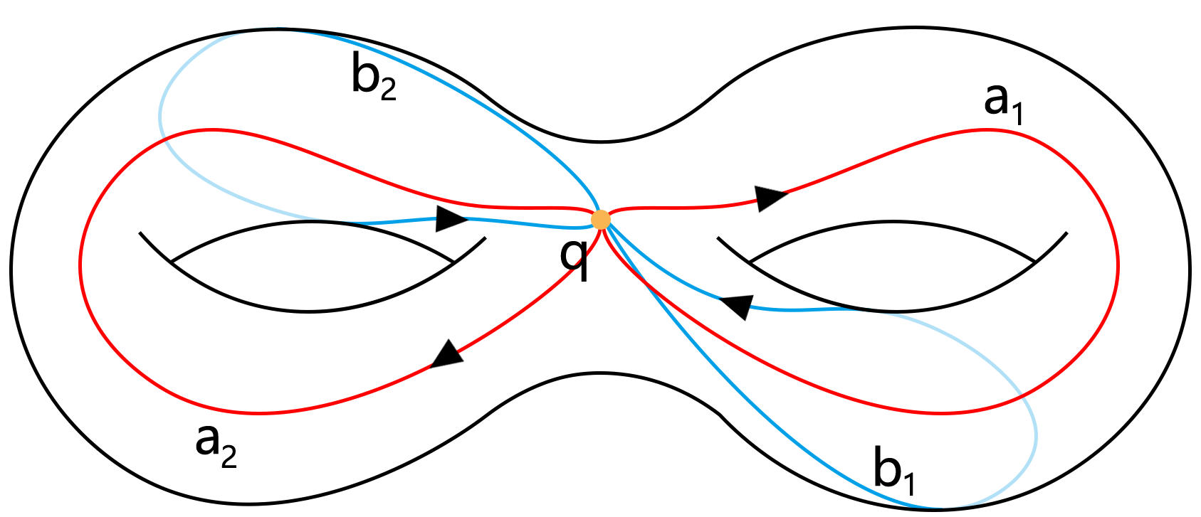
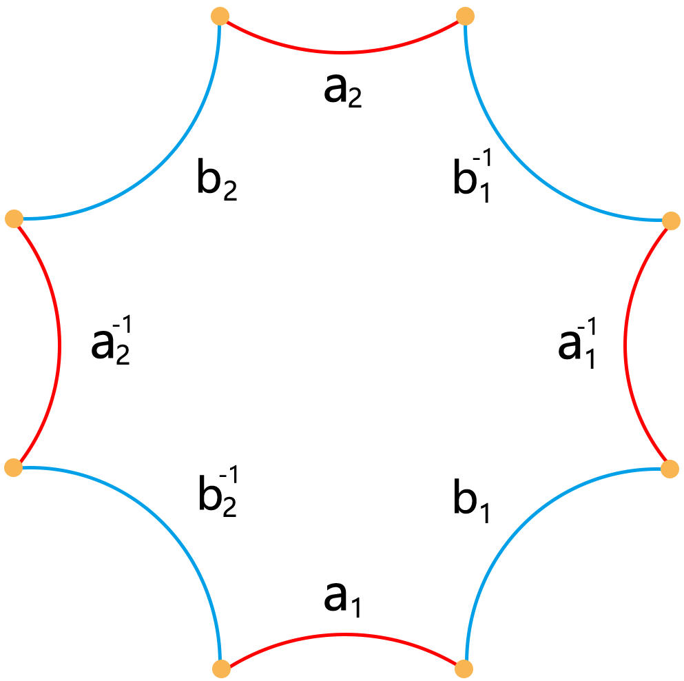
Figure 1: Canonical fundamental group basis.

Suppose $\{a_{1},b_{1},\dots,a_{g},b_{g}\}$ is a set of canonical basis for the homology group $H_{1}(S,\mathbb{Z})$ as shown in Fig. 1. Each $a_{i}$ and $b_{i}$ represent the curves around the inner and outer circumferences of the $i$th handle.

Let $\{\omega_{1},\omega_{2},\dots,\omega_{g}\}$ be a normalized basis of $\Omega^{1}$, the linear space of all holomorphic 1-forms over $\mathbb{C}$. The choice of basis is dependent on the homology basis chosen above; the normalization signifies that

$$\int_{a_{i}}\omega_{j}=\delta_{ij},\quad i,j=1,2,\dots,g.$$

For each curve $\gamma$ in the homology group, we can associate a vector $\lambda_{\gamma}$ in $\mathbb{C}^{g}$ by integrating each of the $g$ 1-forms over $\gamma$,

$$\lambda_{\gamma}=\left(\int_{\gamma}\omega_{1},\int_{\gamma}\omega_{2},\dots,\int_{\gamma}\omega_{g}\right)$$

We define a $2g$-real-dimensional lattice $\Lambda$ in $\mathbb{C}^{g}$,

$$\Gamma=\left\{\sum_{i=1}^{g}s_{i}~{}\lambda_{a_{i}}+\sum_{j=1}^{g}t_{j}~{}\lambda_{b_{j}},\quad s_{i},t_{j}\in\mathbb{Z}\right\}$$

Definition 3.8 (Jacobian).

The Jacobian of the Riemann surface $S$, denoted $J(S)$, is the compact quotient $\mathbb{C}^{g}/\Lambda$.

Definition 3.9 (Abel-Jacobi Map).

Fix a base point $p_{0}\in S$. The Abel-Jacobi map is a map $\mu:S\to J(S)$. For every point $p\in S$, choose a curve $c$ from $p_{0}$ to $p$; the Abel-Jacobi map $\mu$ is defined as follows:

$$\mu(p)=\left(\int_{p_{0}}^{q}\omega_{1},\int_{p_{0}}^{q}\omega_{2},\dots,\int_{p_{0}}^{q}\omega_{g}\right)~{}~{}\mod\Lambda,$$

where the integrals are all along $c$.

It can be shown $\mu(p)$ is well-defined, that the choice of curve $c$ doesn’t not affect the value of $\mu(p)$.

Theorem 3.10 (Abel-Jacobian).

Let $D$ be an divisor of degree $0$ on $S$, then $D$ is the divisor of a meromorphic function $f$ if and only if $\mu(D)=0$ in the Jacobian $J(S)$.

3.3 Quad-Meshes and Meromorphic Quartic Forms

We summarize the intrinsic relation between a quad-mesh and a meromorphic quartic differential.

Definition 3.11 (Quadrilateral Mesh).

Suppose $\Sigma$ is a topological surface, $\mathcal{Q}$ is a cell partition of $\Sigma$, if all cells of $\mathcal{Q}$ are topological quadrilaterals, then we say $(\Sigma,\mathcal{Q})$ is a quadrilateral mesh.

On a quad-mesh, the topological valence of a vertex is the number of faces adjacent to the vertex.

Definition 3.12 (Singularity).

Suppose $(S,\mathcal{Q})$ is a quadrilateral mesh. If the topological valence of an interior vertex is $4$, then we call it a regular vertex, otherwise a singularity; if the topological valence of a boundary vertex is $2$, then we call it a regular boundary vertex, otherwise a boundary singularity. The index of a singularity is defined as follows:

$$\text{Ind}(v_{i})=\left\{\begin{array}[]{lcl}4-\text{val}(v_{i})&v_{i}\not\in\partial(S,\mathcal{Q})\\ 2-\text{val}(v_{i})&v_{i}\in\partial(S,\mathcal{Q})\\ \end{array}\right.$$

where $\text{Ind}(v_{i})$ and $\text{val}(v_{i})$ are the index and the topological valence of $v_{i}$.

Theorem 3.13 (Qaud-Mesh to Meromrophic Quartic Differential).

Suppose $(\Sigma,\mathcal{Q})$ is a closed quadrilateral mesh, then

1. the quad-mesh $\mathcal{Q}$ induces a conformal atlas $\mathcal{A}$, such that $(\Sigma,\mathcal{A})$ form a Riemann surface, denoted as $S_{Q}$.

2. the quad-mesh $\mathcal{Q}$ induces a quartic differential $\omega_{Q}$ on $S_{Q}$. The valence-$k$ singular vertices correspond to poles or zeros of order $k-4$. Furthermore, the trajectories of $\omega_{Q}$ are finite.

Theorem 3.14 (Quartic Differential to Quad-Mesh).

Suppose $(\Sigma,\mathcal{A})$ is a Riemann surface, $\omega$ is a meromorphic quartic differential with finite trajectories, then $\omega$ induces a quadrilateral mesh $\mathcal{Q}$, such that the poles or zeros with order $k$ of $\omega$ corresponds to the singular vertices of $\mathcal{Q}$ with valence $k+4$.

Theorem 3.15 (Quad-mesh singularity Abel-Jacobian condition).

Suppose $\mathcal{Q}$ is a closed quadrilateral mesh, $S_{Q}$ is the induced Riemann surface, $\omega_{Q}$ is the induced meromorphic quadric form. Assume $\omega_{0}$ is an arbitrary holomorphic 1-form on $S_{Q}$, then

$$\mu((\omega_{Q})-4(\omega_{0}))=0\quad\mod\Lambda$$ (3)

in the Jacobian $J(S_{Q})$.

4 Computational Algorithms

This section explains the algorithm in details. The input surface is represented as a triangle mesh $\Sigma$; the output is a meromorphic quartic differential $\omega$, and the flat metric with cone singularities at the poles and zeros induced by $\omega$. The pipeline of the algorithm is as follows:

1. Compute the homology group generators of $\Sigma$, $\{a_{1},\cdots,a_{g};\ b_{1},\cdots,$ $b_{g}\}$;

2. Compute the dual holomorphic 1-form basis $\{\varphi_{1},\cdots,\varphi_{g}\}$; Construct a holomorphic differential $\varphi$ on the Riemann surface $\Sigma$ through a linear combination of basis $\{\varphi_{k}\}_{k=1}^{g}$, locate the zeros of $\varphi$;

3. Compute the period matrix $(A,B)$ of surface and construct the lattice $\Gamma$, Jacobian variet $J(\Sigma)$;

4. Compute Abel-Jacobi map of a given divisor $D$ in the Jacobian variet $J(\Sigma)$;

5. Optimize the divisor $D$ to satisfy the Abel-Jacobian condition;

6. Compute the flat metric with cone singularities at the divisor $D$ by surface Ricci Flow;

7. Compute the cut-graph connecting all singularities; slice the surface along the cut-graph; And isometrically immerse the surface into complex plane; the immersion pulls $(dz)^{4}$ back to the surface and produces a meromorphic quartic differential $\omega$.

8. Trace the critical horizontal and vertical trajectories of $\omega$, namely isoparametric curves through singularities, to generate a T-mesh and partition the surface into rectangular patches.

In the following, we explain every step in details. Each subsection corresponds to one step.

4.1 Homology group basis

In practice, we compute a special set of canonical homology group basis, the tunnel loops $\{a_{i}\}$ and handle loops $\{b_{i}\}$, such that each $a_{i}$ and $b_{i}$ intersect each other at one point. Our algorithm is mainly based on the work of Dey et al, which avoid tetrahedral tessellation and modification of the original triangle mesh. The algorithm utilizes the concept of reeb graph and the linking number to produce different sets of homology basis.

As shown in Fig. 2 left frame, the algorithm may generate homology basis which doesn’t satisfy the intersection condition,

$$a_{i}\cdot b_{j}=\delta_{ij},~{}a_{i}\cdot a_{j}=0,~{}b_{i}\cdot b_{j}=0,\quad i,j=1,\dots,g,$$ (4)

where $\alpha\cdot\beta$ represents the algebraic intersection number between $\alpha$ and $\beta$, $g$ is the genus of the mesh.

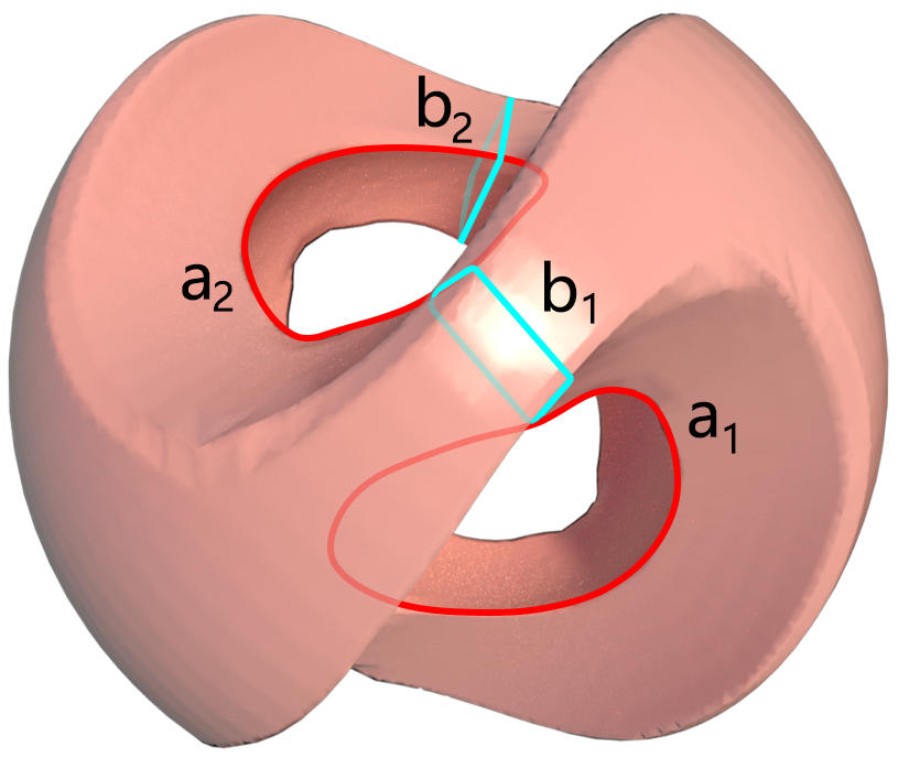
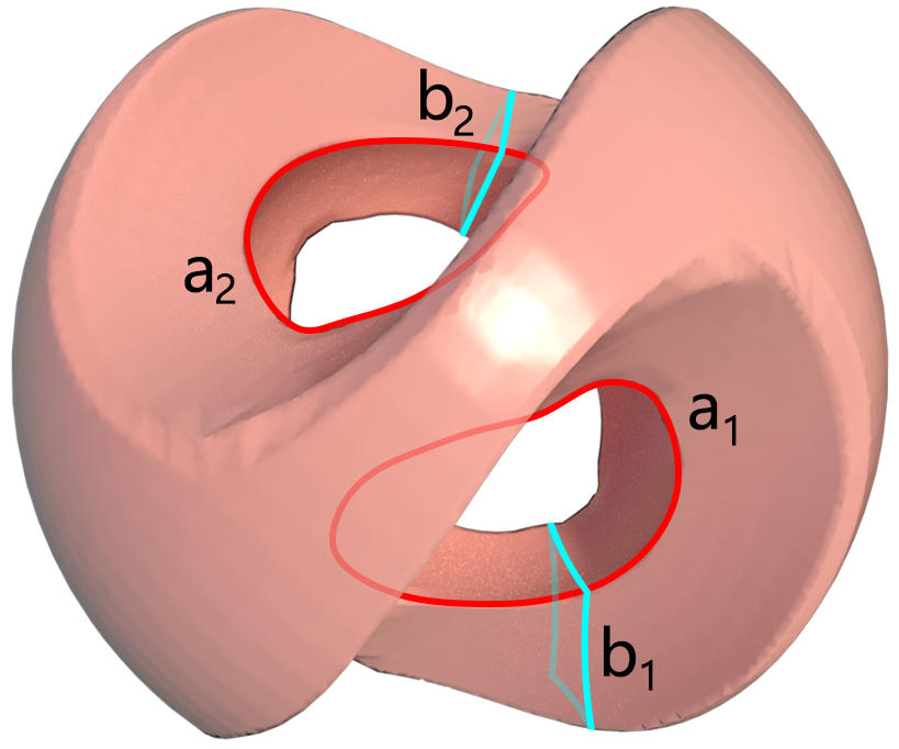
Figure 2: Sculpt model. Left: the handle loop $b_{1}$ intersects both tunnel loops $a_{1}$ and $a_{2}$, where we call the handle loop $b_{1}$ illegal. Right: each handle loop $b_{i}$ only intersects its conjugate $a_{i}$ once.

We compute the algebraic intersection between the tunnel loops and handle loops, if the intersection condition 4 is violated, we randomly reset the height function used for constructing reeb graph, and obtain a new set of handle loops and tunnel loops. After several iterations, we can get a set of canonical homology group basis, as shown in Fig. 2 right frame.

4.2 Holomorphic 1-form Basis

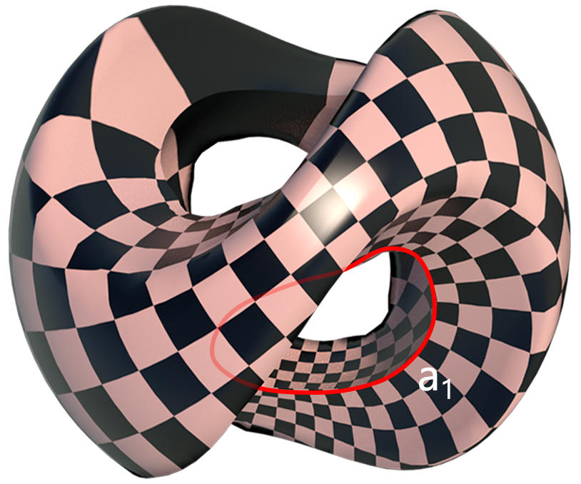
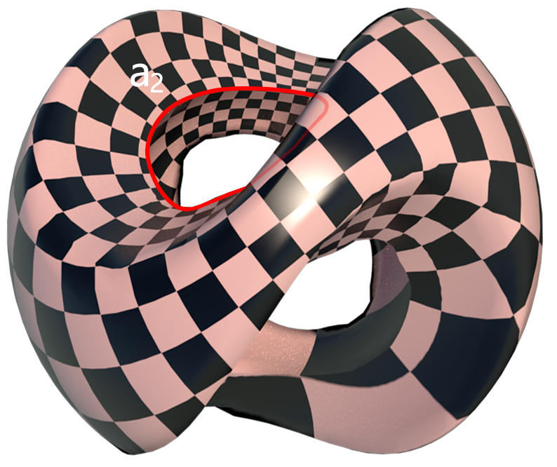
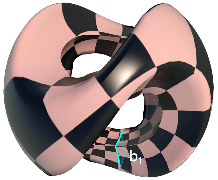
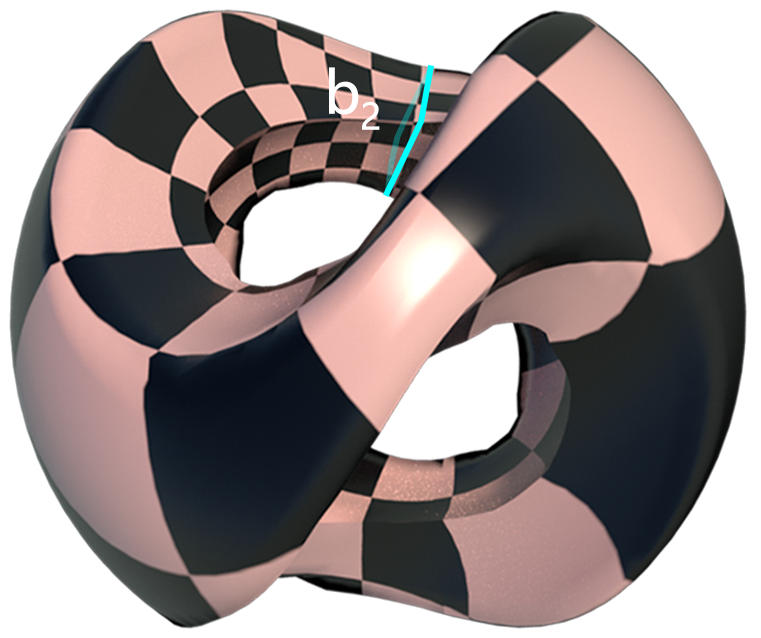
Figure 3: A holomorphic 1-form basis on a genus two surface, the Sculpt model.

The algorithm of computing holomorphic 1-form is based of the work of Gu et al , which is based on Hodge theory. Step 1, for each loop $\gamma$, we slice the mesh $M$ along $\gamma$ to get an open mesh $\bar{M_{\gamma}}$ with boundaries $\partial M_{\gamma}=\gamma^{+}-\gamma^{-}$, then we construct a function

$$g_{\gamma}(v_{i})=\left\{\begin{array}[]{ll}1&v_{i}\in\gamma^{+}\\ 0&v_{i}\in\gamma^{-}\\ \text{rand}&\text{otherwise}\end{array}\right.$$

Then the discrete 1-form $\lambda_{\gamma}=dg_{\gamma}$ is a closed 1-form. In this way, we construct a set of cohomology group basis $\lambda_{a_{1}},\lambda_{b_{1}},\cdots,\lambda_{a_{g}},\lambda_{b_{g}}$. Step 2, for each closed 1-form $\lambda$, we construct a function $f:M\to\mathbb{R}$, such that $\lambda+df$ is harmonic, namely the function $f$ satisfies the Poisson equation $\Delta f=-\delta\lambda$. In this way, we diffuse cohomology basis to harmonic 1-form group basis, denoted as $\omega_{a_{1}},\omega_{b_{1}},\cdots,\omega_{a_{g}},\omega_{b_{g}}$. Step 3, each harmonic 1-form $\omega$ is equivalent to a curl-free vector field on $M$, we rotate the vector field by $\frac{\pi}{2}$ about the normal to the surface to obatin a divergence free vector field, which is equivalent to another harmonic 1-form ${}^{*}\omega$. The pair $\omega+\sqrt{-1}{}^{*}\omega$ is a holomorhic 1-form. In this way, we construct the holomorphic 1-form basis $\{\varphi_{a_{1}},\varphi_{b_{1}},\dots,\varphi_{a_{g}},\varphi_{b_{g}}\}$, where

$$\varphi_{\gamma}=\omega_{\gamma}+\sqrt{-1}{}^{*}\omega_{\gamma},\gamma\in\{a_{1},\dots,a_{g},b_{1},\dots,b_{g}\}.$$

According to the Riemann-Roch theory, the above set of holomorphic 1-forms span the linear space of all holomorphic 1-forms $\Omega$, namely for any $\varphi\in\Omega$,

$$\varphi=\sum_{k=1}^{g}\alpha_{k}\varphi_{a_{k}}+\sum_{l=1}^{g}\beta_{l}\varphi_{b_{l}},$$

where the $\alpha_{k}$, $\beta_{l}$ are real linear combination coefficients.

In practice, in order to compute the zeros of $\varphi$ more accurately, we choose the linear combination coefficients, such that the conformal factor function of $\varphi$ is as uniform as possible. In our implementation, we assign all $\alpha_{k}$’s and $\beta_{l}$’s to be $1$. Heuristically, the resulting holomorphic 1-form meets our accuracy requirement.

4.3 Period matrix and Lattice

We can further construct a set of holomorphic 1-form basis $\{\varphi_{1},\varphi_{2},\dots,\varphi_{g}\}$, such that

$$\int_{a_{i}}\varphi_{j}=\delta_{ij},i,j=1,2,\dots,g.$$

Then for each $\gamma$ in the homology basis, we construct a $g$ dimensional vector $\lambda_{\gamma}\in\mathbb{C}^{g}$,

$$\lambda_{\gamma}=\left(\int_{\gamma}\varphi_{1},\int_{\gamma}\varphi_{2},\cdots,\int_{\gamma}\varphi_{g}\right)$$

The period matrix $(A,B)$ can be constructed as

$$A=\begin{bmatrix}\int_{a_{1}}\varphi_{1}&\int_{a_{2}}\varphi_{1}&\cdots&\int_{a_{g}}\varphi_{1}\\ \int_{a_{1}}\varphi_{2}&\int_{a_{2}}\varphi_{2}&\cdots&\int_{a_{g}}\varphi_{2}\\ \vdots&\vdots&\ddots&\vdots\\ \int_{a_{1}}\varphi_{g}&\int_{a_{2}}\varphi_{g}&\cdots&\int_{a_{g}}\varphi_{g}\\ \end{bmatrix}~{}B=\begin{bmatrix}\int_{b_{1}}\varphi_{1}&\int_{b_{2}}\varphi_{1}&\cdots&\int_{b_{g}}\varphi_{1}\\ \int_{b_{1}}\varphi_{2}&\int_{b_{2}}\varphi_{2}&\cdots&\int_{b_{g}}\varphi_{2}\\ \vdots&\vdots&\ddots&\vdots\\ \int_{b_{1}}\varphi_{g}&\int_{b_{2}}\varphi_{g}&\cdots&\int_{b_{g}}\varphi_{g}\\ \end{bmatrix}$$ (5)

by our construction $A$ is the $g\times g$ identity matrix. Then we construct a lattice $\Gamma$ in $\mathbb{C}^{g}$,

$$\Gamma=\left\{\sum_{k=1}^{g}(s_{k}\lambda_{a_{k}}+t_{k}\lambda_{b_{k}},\quad s_{k},t_{k}\in\mathbb{Z}\right\}$$

4.4 Abel-Jacobi Map

Given a canonical homology group basis we slice the surface along the basis to obtain a topological disk $\bar{M}$. Fix a base point in the interior of $\bar{M}$,$p_{0}\in\bar{M}$, for any point $p\in M$, we can choose arbitrarily a path $\gamma\subset\bar{M}$ connecting $p$ and $p_{0}$, the Abel-Jacobi map $\mu:M\to J(M)$, $J(M)=\mathbb{C}^{g}/\Gamma$, is defined as

$$\mu(p)=\Phi(p)~{}\mod~{}\Gamma,$$

where

$$\Phi(p)=\left(\int_{\gamma}\varphi_{1},\int_{\gamma}\varphi_{2},\cdots,\int_{\gamma}\varphi_{g}\right)^{T}.$$ (6)

Similarly, given a divisor $D=\sum_{i=1}^{n}n_{i}p_{i}$,

$$\mu(D)=\sum_{i=1}^{n}n_{i}\mu(p_{i})=\sum_{i=1}^{n}n_{i}\left(\int_{p_{0}}^{p_{i}}\varphi_{1},\int_{p_{0}}^{p_{i}}\varphi_{2},\cdots,\int_{p_{0}}^{p_{i}}\varphi_{g}\right)^{T}~{}\mod~{}\Gamma.$$

Abel-Jacobi condition claims that if $D$ is a principle divisor, then $\mu(D)$ is $0$, namely

$$\Phi(D)-A\begin{bmatrix}s_{1}\\ \vdots\\ s_{g}\end{bmatrix}-B\begin{bmatrix}t_{1}\\ \vdots\\ t_{g}\end{bmatrix}=\begin{bmatrix}0\\ \vdots\\ 0\end{bmatrix}$$ (7)

By expansion, we obtain the equation

$$\begin{split}\@add@centering\centering\left[\begin{array}[]{c}\mathop{\sum}_{i=1}^{n}n_{i}\bigintss_{\gamma_{i}}\varphi_{1}\\ \mathop{\sum}_{i=1}^{n}n_{i}\bigintss_{\gamma_{i}}\varphi_{2}\\ \quad\vdots\\ \mathop{\sum}_{i=1}^{n}n_{i}\bigintss_{\gamma_{i}}\varphi_{g}\end{array}\right]\ -\ \begin{bmatrix}\mathop{\sum}_{k=1}^{g}(s_{k}\bigintss_{a_{k}}\varphi_{1}+t_{k}\bigintss_{b_{k}}\varphi_{1})\\ \mathop{\sum}_{k=1}^{g}(s_{k}\bigintss_{a_{k}}\varphi_{2}+t_{k}\bigintss_{b_{k}}\varphi_{2})\\ \vdots\\ \mathop{\sum}_{k=1}^{g}(s_{k}\bigintss_{a_{k}}\varphi_{g}+t_{k}\bigintss_{b_{k}}\varphi_{g})\end{bmatrix}=\begin{bmatrix}0\\ 0\\ \vdots\\ 0\end{bmatrix},\end{split}$$ (8)

where $s_{k}$, $t_{k}$ are integers, $\gamma_{i}$ is the path connecting $p_{0}$ and $p_{i}$ in $\bar{M}$.

4.5 Abel-Jacobian Condition Optimization System

Suppose we are given an initial divisor $D_{0}$, if it doesn’t satisfy the Gauss-Bonnet condition, namely $\deg(D_{0})\neq 8g-8$, then we can add extra poles or zeros to modify $D_{0}$ to $D=\sum_{i=1}^{k}n_{i}p_{i}$, such that $\deg(D)=8g-8$. We choose a holomorphic 1-form $\varphi$.

First, we determine the integer coefficients $s_{k}$ and $t_{k}$ in Abel-Jacobi condition (8) by minimizing the norm

$$\min_{s_{k},t_{k}\in\mathbb{Z}}\left\|\Phi(D)-\sum_{k=1}^{g}s_{k}\lambda_{a_{k}}-\sum_{k=1}^{g}t_{k}\lambda_{b_{k}}-\Phi(4(\varphi))\right\|^{2},$$ (9)

this can be accomplished by standard integer programming .

Second, once the integer coefficients $s_{k},t_{k}$, $k=1,2,\dots,g$ are set, we further minimize the squared norm of $\mu(D)$ with respect to the positions of poles and zeros,

$$\min_{p_{1},\dots p_{k}\in M}\left\|\Phi(D)-\sum_{k=1}^{g}s_{k}\lambda_{a_{k}}-\sum_{k=1}^{g}t_{k}\lambda_{b_{k}}-\Phi(4(\varphi))\right\|^{2}.$$

Let $d\in\mathbb{C}^{g}$ be

$$d=\sum_{k=1}^{g}s_{k}\lambda_{a_{k}}-\sum_{k=1}^{g}t_{k}\lambda_{b_{k}}-\Phi(4(\varphi)),$$

then the above energy becomes

$$E(p_{1},\dots,p_{k}):=\sum_{j=1}^{g}\left\|\sum_{i=1}^{k}n_{i}\int_{p_{0}}^{p_{i}}\varphi_{j}-d_{j}\right\|^{2}.$$

For each point $p_{i}$, we choose a local neightborhood $\Delta_{i}$ of $p_{i}$, with local parameter $z_{i}$, then the holomorphic 1-form $\omega_{j}$ has local representation,

$$\varphi_{j}=h_{j}^{i}(z_{i})dz_{i},$$

where $h_{j}^{i}(z_{i})$ is a holomorphic function defined on $\Delta_{i}$.

$$\frac{\partial E}{\partial p_{i}}=\sum_{j=1}^{g}\left[n_{i}h_{j}^{i}(p_{i})\left(\sum_{i=1}^{k}n_{i}\int_{p_{0}}^{p_{i}}\bar{\varphi}_{j}-\bar{d}_{j}\right)+n_{i}\bar{h}_{j}^{i}(p_{i})\left(\sum_{i=1}^{k}n_{i}\int_{p_{0}}^{p_{i}}\varphi_{j}-d_{j}\right)\right],$$ (10)

we can use gradient descent method to minimize $\|\mu(D)\|^{2}$. In practice, we choose the triangle face containing $p_{i}$ as $\Delta_{i}$. We isometrically embed $\Delta_{i}$ onto the plane, and the planar coordinates give local parameter $z_{i}$. $\omega_{j}$ can be represented as a complex linear function on $\Delta_{i}$, which is $h_{j}^{i}(z_{i})$. In this way, we can minimize the squared norm of $\mu(D)$.

The algorithm is presented briefly in Alg. 1.

Algorithm 1 Optimize a Divisor to Satisfy the Abel-Jacobi Condition

0:  Closed mesh $M$; A group of singularities $D$; A holomorphic 1-form; Precision threshold $\varepsilon$.

0:  Optimized divisor $D$ Abel-Jacobian condition.

1:  if $D$ doesn’t satisfy Gauss-Bonnet Condition then

2:     Locate the vertices on $M$ with local maximal Gaussian curvature as poles, or with local minimal curvature as zeros;

3:     Add these vertices to the divisor $D$, such that $D$ satisfies the Gauss-Bonnet condition.

4:  end if

5:  Locate the zeros of $\varphi$ to obtain the divisor $(\varphi)$;

6:  Compute $\Phi(D)$ and $\Phi(4(\varphi))$ using Eqn. 6;

7:  Compute the Abel-Jacobi $\mu(D-4(\varphi))$map by optimization using integer programming Eqn.9;

8:  while  $\|\mu(D-4(\varphi))\|^{2}>\varepsilon$  do

9:     for All each pole and zero $p_{i}$ in $D$  do

10:        Locate the face $\Delta_{i}$ containing $p_{i}$;

11:        Compute the local representation $\varphi_{j}(z_{i})=h_{j}^{i}(z_{i})dz_{i}$;

12:        Compute the gradient of the energy Eqn. 10;

13:     end for

14:     Update the poisitions of the singularities $p_{i}\leftarrow p_{i}-\partial\nabla E/\partial p_{i}$;

15:     Recompute the Abel-Jacobi map $\mu(D-4(\varphi))$;

16:  end while

17:  return  The divisor $D$.

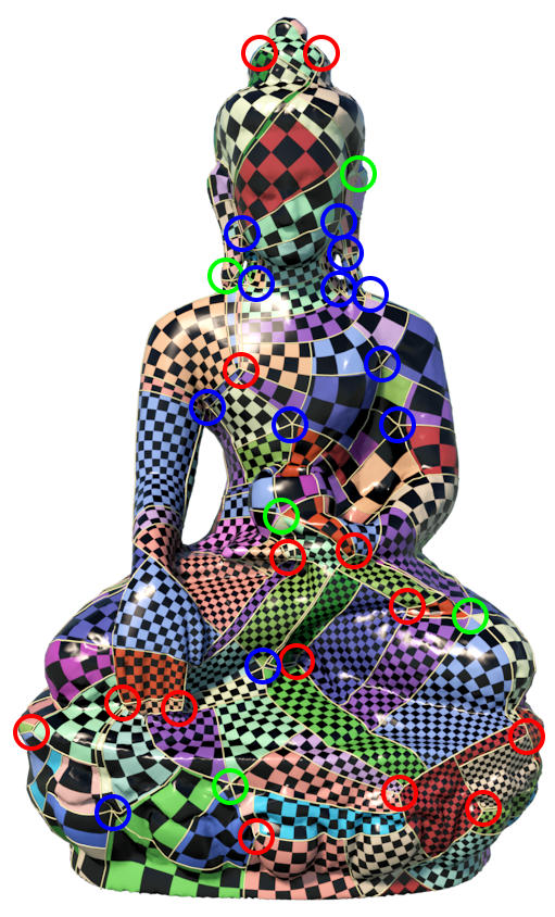
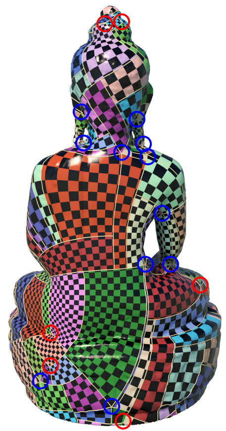
Figure 4: The singularities of the Buddha surface.

Fig. 4 shows the singularities on the Buddha surface satisfying the Abel-Jacobi condition.

4.6 Discrete Surface Ricci Flow

Once the divisor $D=\sum_{i=1}^{k}n_{i}p_{i}$ is obtained, we can set the target curvature as

$$\bar{K}(v_{i})=\left\{\begin{array}[]{ll}(4-n_{i})\frac{\pi}{2}&v_{i}\in D\\ 0&\text{otherwise}\end{array}\right.$$

For each vertex $v_{i}\in M$, we set the initial conformal factor as $u_{i}=0$. Then the edge length is given by vertex scaling, for edge $e_{ij}=[v_{i},v_{j}]$, its length is given by

$$l_{ij}=e^{u_{i}}\beta_{ij}e^{u_{j}},$$

where $\beta_{ij}$ is the initial edge length. The corner angles are calculated using Euclidean cosine law,

$$\theta_{k}^{ij}=\cos^{-1}\frac{l_{ik}^{2}+l_{jk}^{2}-l_{ij}^{2}}{2l_{ik}l_{jk}},$$

the discrete Gaussian curvature is given by

$$K(v_{i})=\left\{\begin{array}[]{rl}2\pi-\sum_{jk}\theta_{i}^{jk}&v_{i}\not\in\partial M\\ \pi-\sum_{jk}\theta_{i}^{jk}&v_{i}\in\partial M\end{array}\right.$$

The discrete Ricci energy is defined as

$$E(u_{1},\dots,u_{n})=\int^{(u_{1},\dots,u_{n})}\sum_{i=1}^{n}(\bar{K}_{i}-K_{i})du_{i}.$$

The gradient of the energy is given by

$$\nabla E=(\bar{K}_{1}-K_{1},\bar{K}_{2}-K_{2},\cdots,\bar{K}_{n}-K_{n})^{T}.$$

The Hessian matrix is given by the cotange edge weight

$$\frac{\partial^{2}E}{\partial u_{i}\partial u_{j}}=\left\{\begin{array}[]{lr}(\cot\theta_{k}^{ij}+\cot\theta_{l}^{jl})/2&e_{ij}\not\in\partial M\\ \cot\theta_{k}^{ij}/2&e_{ij}\in\partial M\end{array}\right.$$

and

$$\frac{\partial^{2}E}{\partial u_{i}^{2}}=-\sum_{j\neq i}\frac{\partial^{2}E}{\partial u_{i}\partial u_{j}}.$$

We can use Newton’s method to optimize the Ricci energy, during the optimization, we update the triangulation to be Delaunay all the time. The convergence is proven in the work . We can compute holonomy using the resulting Riemannian metric.

4.7 Isometric Immersion and Meromorphic Quartic Differential

We have obtain a set of canonical homology group basis $\{a_{1},\dots,a_{g},b_{1},\dots,b_{g}\}$. The union of the basis form a cut graph $\Gamma$ of the mesh. For each pole or zero $p_{i}$ in $D$, we find a shortest path $\gamma_{i}$ connecting $p_{i}$ to the cut graph, furthermore, all such shortest paths $\gamma_{i}$’s are disjoint. Then we slice $M$ along the cut graph and the shortest paths, $\Lambda\bigcup\{\bigcup_{i=1}^{k}\gamma_{i}\}$, to obtain a topological disk $\tilde{M}$.

Then we flatten $\tilde{M}$ face by face using the metric obtained by the discrete surface Ricci flow. This produces an immersion of $\varphi:\tilde{M}\to\mathbb{C}$. On the complex plane, there is a canonical differential $dz^{4}$, the pull back $\varphi^{*}dz^{4}$ is a meromorphic quartic differential defined on $M$. We can use $\tau$ as a parameterization, and use checker board texture mapping to visualize the quartic differential.

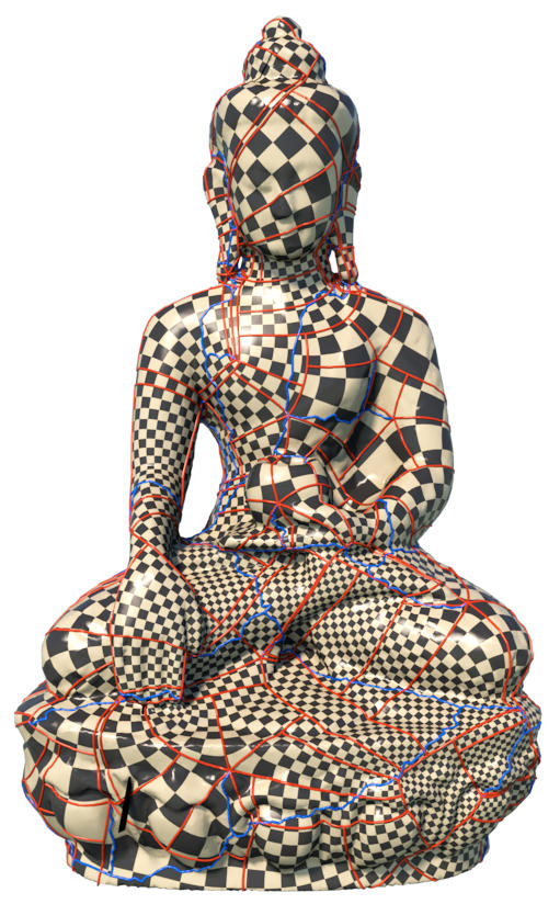
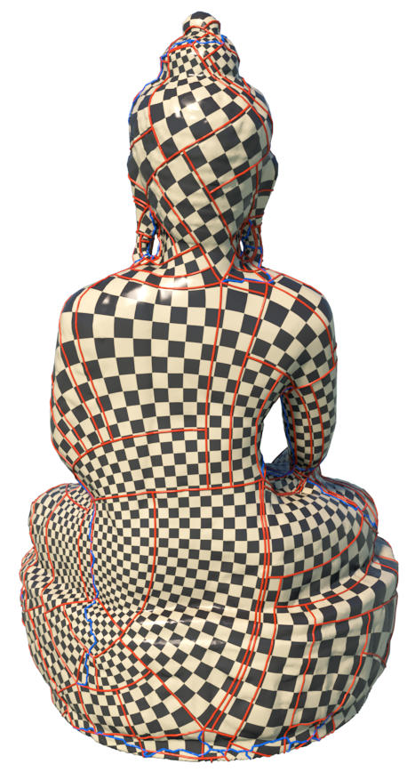
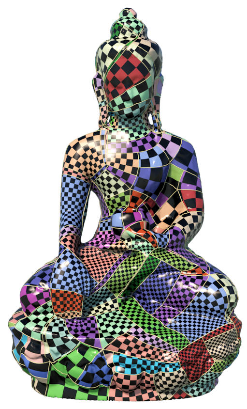
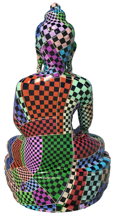
Figure 5: In the left two frames, the red curves form the motor-graph, the blue curves are the original cut graph. The right two frames show the T-Mesh of the Buddha surface.

4.8 T-Mesh Generation

We trace the critical trajectories of the meomorphic quadratic differential $\varphi^{*}dz^{4}$, denoted as $\{\gamma_{1}(s_{1}),\gamma_{2}(s_{2}),\cdots,\gamma_{n}(s_{n})\}$, where $s_{k}$ is the arc length parameter of $\gamma_{k}$, their images $\varphi(\gamma_{k})$’s are the horizontal and vertical lines through the zeros and poles on the parameter plane. If $\gamma_{i}(s_{i})$ intersects $\gamma_{j}(s_{j})$ at $p$, if $s_{i}<s_{j}$, then $\gamma_{j}$ stops at $p$, $\gamma_{i}$ continues. This procedure will generate the motor graph on the surface, as shown in the left two frames in Fig. 5.

The surface is partitioned into rectangular patches as shown in the right two frames of Fig. 5. Each surface patch is parameterized to a planar rectangle, as shown in Fig. 6. The corresponding surface patch and the planar rectangle are rendered using the same color.

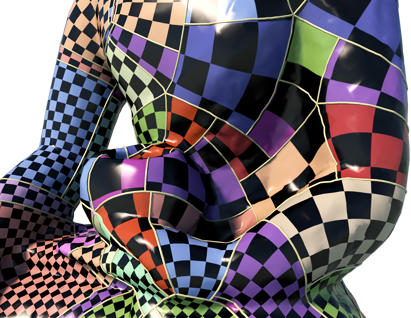
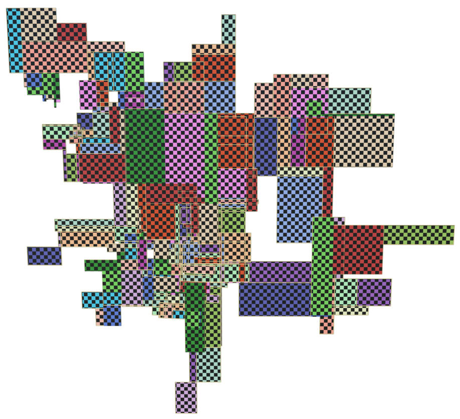
(a) zoomed in	(b) planar images

Figure 6: Each surface patch is parameterized to a planar rectangle.

5 Experimental Results

In this section, we briefly report our experimental results. All the experiments were conducted on a PC with 1.60GHz Intel(R) core(TM) i5-8250U CPU, 1.60GB RAM and 64-bit Windows 10 operating system. The running time is reported in table 1.

5.1 T-Mesh Generation

The singularities and the resulting T-meshes are illustrated in the figures. As shown in Fig. 7, the singularities surrounded by red, blue and green circles represent the indices $+1$, $-1$ and $-2$ respectively. The points surrounded by white circles are the T-junctions of the T-mesh. Different surface patches are color-encoded differently. By carefully examining the texture patterns in Fig. 7, we can see that the adjacent patches differ by horizontal and vertical translations composed with rotations by angle $k\frac{\pi}{2}$, $k\in\mathbb{Z}$. Therefore, we can construct T-Splines on these T-meshes directly.

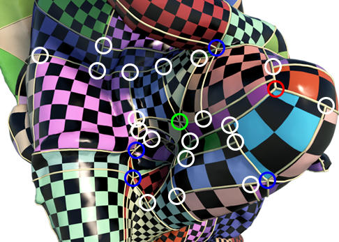
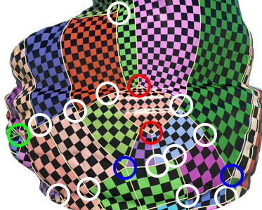
Figure 7: Singularities.

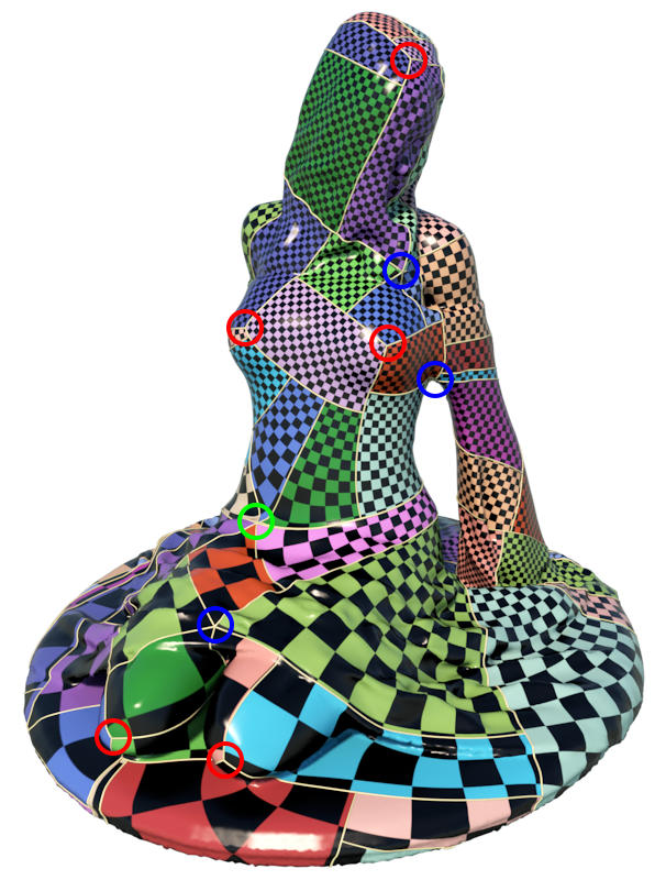
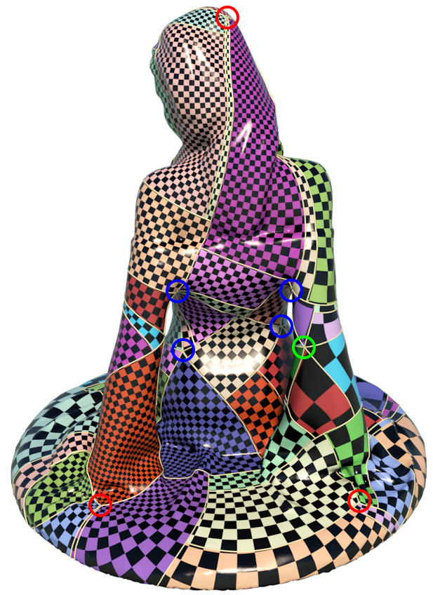
(a) front view	(b) back view

Figure 8: Singularities and the T-Mesh of the Loveme model.

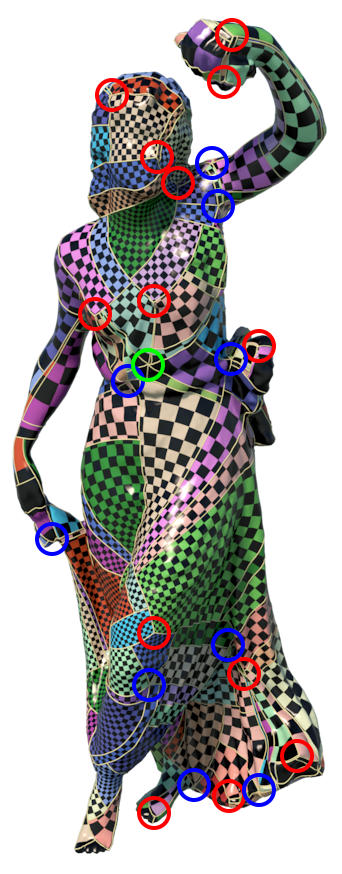
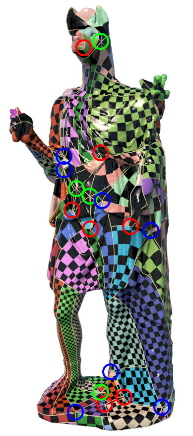
Ornament	Dancer	Hermanubis

Figure 9: Singularities and the T-meshes of high genus surfaces.

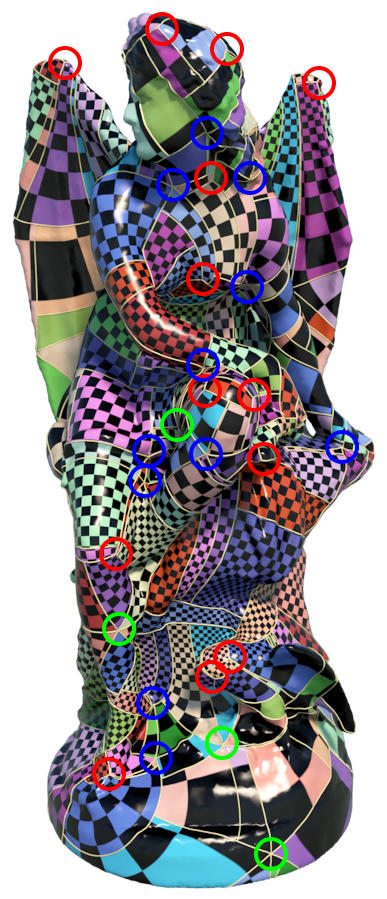
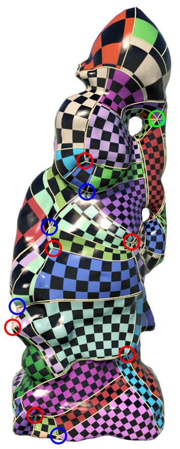
Witch model	Kiss model	Monk model

Figure 10: Singularities and T-Meshes of the surfaces with complicated geometries.

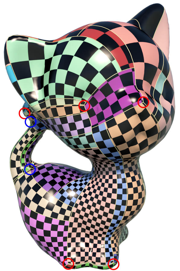
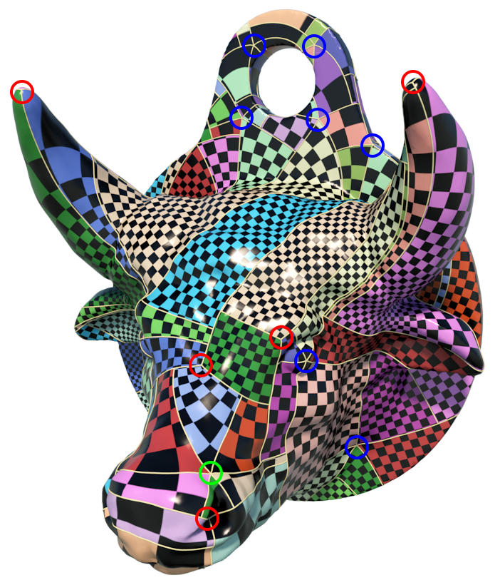
Kitten model	Amphora model	Bull head

Figure 11: Singularities and T-Meshes of various surfaces.

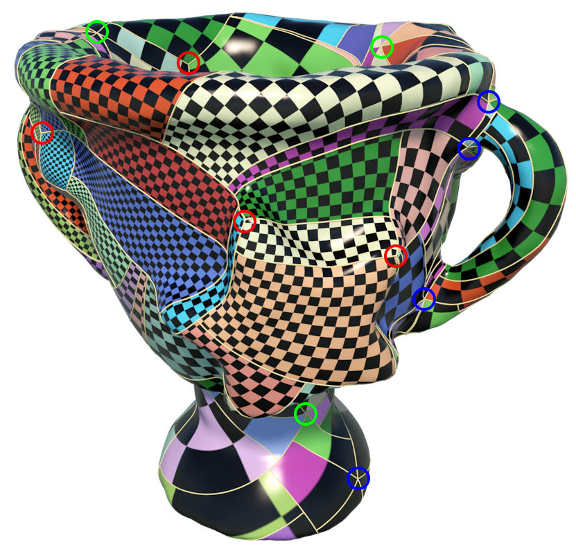
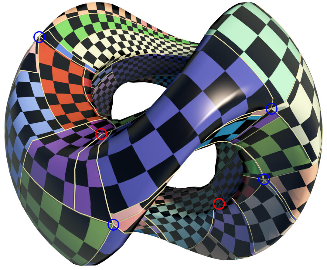
Star cup	Sculpture model

Figure 12: Singularities and T-Meshs of high genus surfaces.

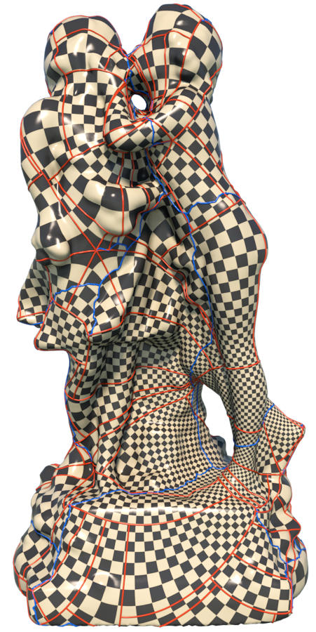
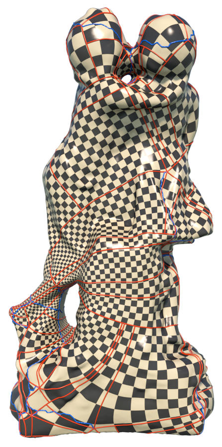
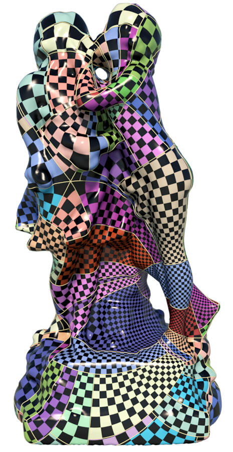
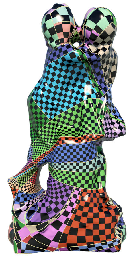
Figure 13: The motor-graph and T-mesh of the genus $3$ 2kids surface.

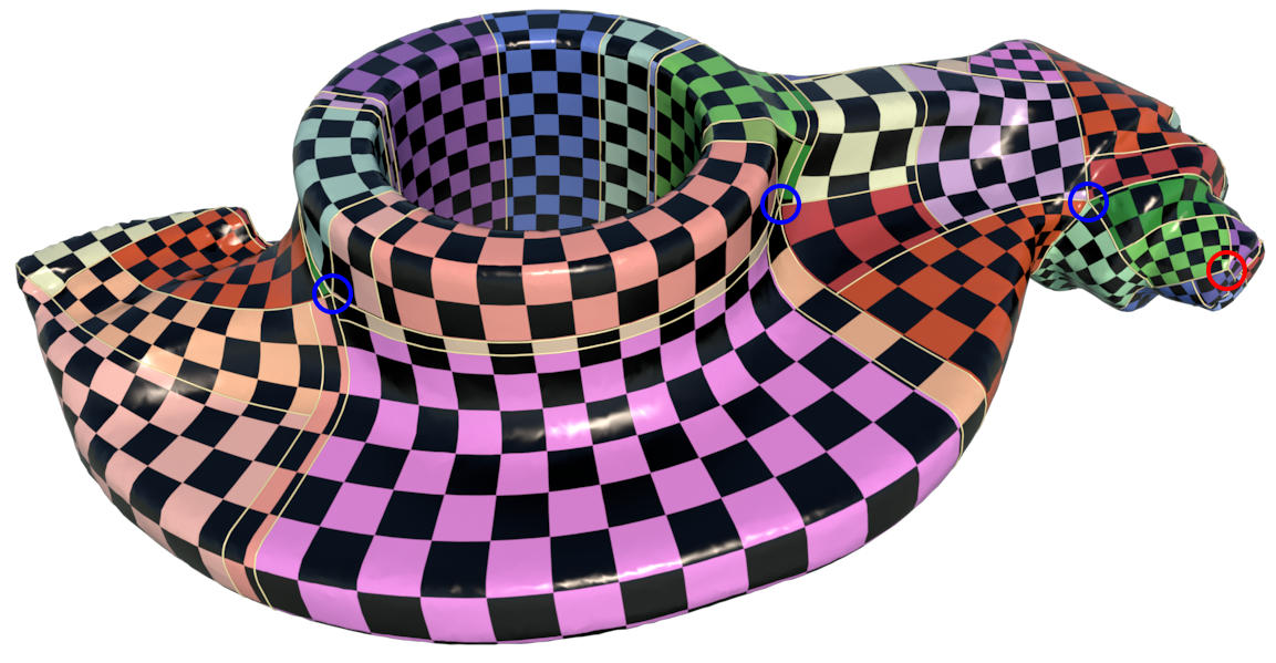
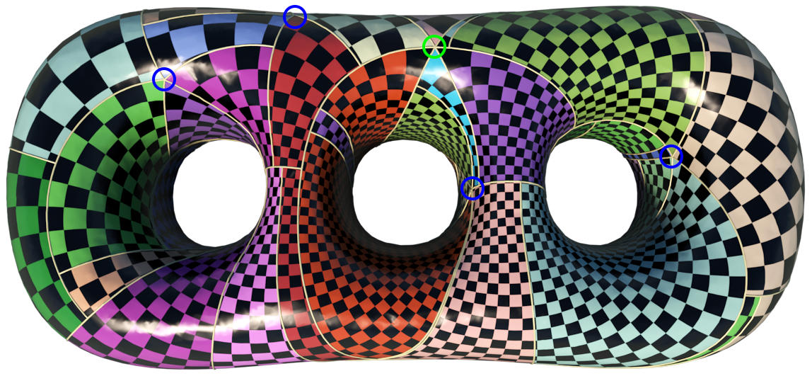
Rocker arm	3 holes surface

Figure 14: Singularities and T-Meshes of high genus surfaces.

Table 1: Runing time

Model	Mesh Information				Holo 1-form	Holo zeros	Legalization of Singularities			Ricci Flow	Iso. Immersion
	a	b	c	d	Time(sec.)	Time(sec.)	Error Threshold	Iterations	Time(sec.)	Time(sec.)	Time(sec.)
Kitten	10.2k	30.7k	20.4k	1	10.247	—	3.0e-4	2132	0.002	0.013	0.006
Ornament	28.8k	86.5k	57.7k	1	47.954	—	3.0e-4	3382	0.005	6.177	0.014
Rockerarm	40.2k	120.5k	80.4k	1	39.014	—	3.0e-4	2049	0.004	12.134	0.021
Dancer	43.0k	129.1k	86.0k	1	43.913	—	3.0e-4	6069	0.005	10.0659	0.027
Bull	75.8k	227.3k	151.5k	1	95.904	—	3.0e-4	2313	0.003	18.160	0.054
Sculpt	4.0k	12.2k	8.0k	2	4.828	0.029	1.0e-3	37601	0.052	1.485	0.002
Starcup	30.0k	90.0k	60.0k	2	51.682	0.301	3.0e-4	1167	0.005	6.654	0.013
Monk	38.5k	115.5k	77.0k	2	86.741	4.037	3.0e-4	17551	0.108	8.624	0.022
Hermanubis	39.9k	119.8k	79.9k	2	96.122	1.441	3.0e-4	17540	0.043	10.370	0.025
Amphora	82.6k	246.5k	164.3k	2	174.396	0.883	3.0e-4	5129	0.016	21.4288	0.046
Loveme	86.7k	260.2k	173.5k	2	191.663	1.156	3.0e-4	5776	0.020	25.7747	0.0.57
Buddha	59.4k	178.1k	118.7k	3	179.568	2.623	3.0e-4	670539	2.021	13.117	0.026
2Kids	61.7k	185.2k	123.5k	3	201.353	6.274	3.0e-4	94620	0.546	14.633	0.027
3Holes	65.0k	195.0k	130.0k	3	218.954	0.819	1.0e-3	343710	0.9333	16.756	0.032
Witch	75.0k	225.0k	150.0k	4	363.533	10.877	3.0e-4	304729	1.033	20.343	0.051
Hardware	CPU									RAM
	Intel(R) Core(TM) i5-8250U CPU $@$ 1.60GHz									16.0GB

5.2 Abel-Jacobi and Holonomy condition verification

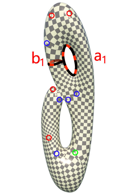
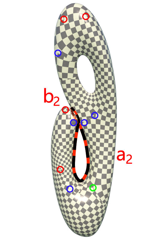
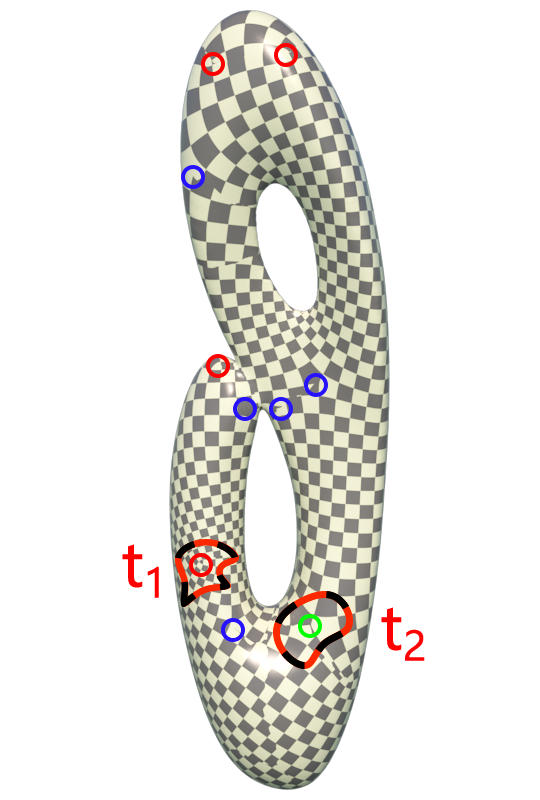
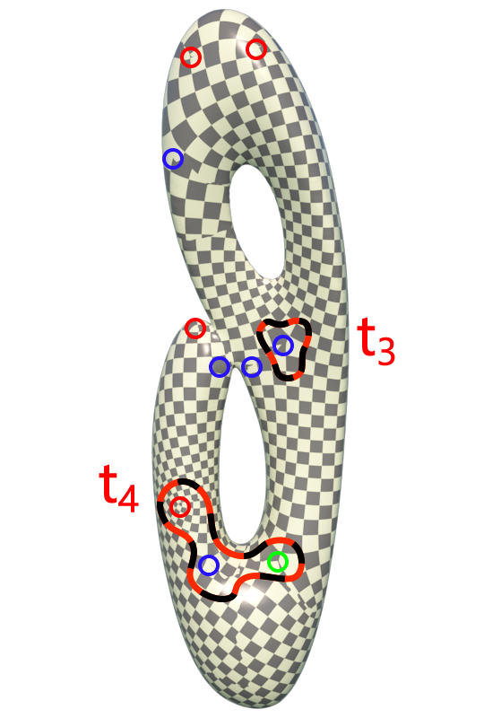
Figure 15: The loops on the genus two Garniture model : $a_{1}$, $a_{2}$ are the tunnel loops; $b_{1}$, $b_{2}$ are the handle loops; $t_{1}$, $t_{2}$, $t_{3}$ surround index $-1$, $+2$, $+1$ singularities, respectively; $t_{4}$ encloses three singularities, with index $+1$, $-1$, $-2$ respectively.

Table 2: Th holonomy of the loops in Fig. 15, rotation components.

Loops	$\mathbf{a_{1}}$	$\mathbf{b_{1}}$	$\mathbf{a_{2}}$	$\mathbf{b_{2}}$
Rotation degree(∘)	90.31809	-0.12269	0.19303	89.81468
Loops	$\mathbf{t_{1}}$	$\mathbf{t_{2}}$	$\mathbf{t_{3}}$	$\mathbf{t_{4}}$
Rotation degree(∘)	270.00047	540.00136	450.00192	539.99818

We verify the holonomy conditon for a genus two surface as shown in Fig. 15. We compute the tunnel loops $a_{1},a_{2}$ and handle loops $b_{1},b_{2}$, and several loops enclosing different number of singularities. The we compute their holonomies by parallel transportation on the flat metric computed using Ricci flow, the rotation components are reported in the table  3. We can see that all the holonomies are very close to $k90^{\circ}$, where $k$ is an integer.

Furthermore, for every surface, we compute the image of the singularities under the Abel-Jacobi map, all the results are reported in table  3. We can see that all the images are very close to the zero point in the Jacobian lattice, this shows the singularities satisfy the Abel-Jacobi condition. This demonstrates the accuracy of our proposed algorithm.

Table 3: Abel Jacobian mapping result

Model	Abel Jacobian Mapping Result
KITTEN	$\begin{pmatrix}\mathbf{\ 2.13971e-04\quad+\quad i\ *\ 7.09315e-05\ }\end{pmatrix}$
ORNAMENT	$\begin{pmatrix}\mathbf{\ -1.09501e-08\quad+\quad i\ *\ 5.73307e-08\ }\end{pmatrix}$
ROCKERARM	$\begin{pmatrix}\mathbf{\ -6.05103e-05\quad+\quad i\ *\ 6.27266e-06\ }\end{pmatrix}$
DANCER	$\begin{pmatrix}\mathbf{\ -3.14143e-05\quad+\quad i\ *\ 1.57991e-05\ }\end{pmatrix}$
BULL	$\begin{pmatrix}\mathbf{\ -1.55144e-05\quad+\quad i\ *\ 6.56513e-06\ }\end{pmatrix}$
SCULPT	$\begin{pmatrix}\mathbf{\ -3.72147e-04\quad-\quad i\ *\ 9.82485e-04\ }\\ \textbf{ \ 8.03122e-04 \quad+ \quad i \ * \ 6.25321e-04 \ }\end{pmatrix}$
STARCUP	$\begin{pmatrix}\mathbf{\ 4.59275e-05\quad-\quad i\ *\ 1.27194e-04\ }\\ \textbf{ \ 8.14751e-05 \quad- \quad i \ * \ 2.32289e-04 \ }\end{pmatrix}$
MONK	$\begin{pmatrix}\mathbf{\ -1.37142e-05\quad-\quad i\ *\ 1.84819e-04\ }\\ \textbf{ \ 4.70251e-05 \quad+ \quad i \ * \ 1.90921e-04 \ }\end{pmatrix}$
HERMANUBIS	$\begin{pmatrix}\mathbf{\ -1.05753e-04\quad-\quad i\ *\ 8.17228e-05\ }\\ \textbf{ \ 9.29236e-05 \quad+ \quad i \ * \ 4.96067e-05 \ }\end{pmatrix}$
AMPHORA	$\begin{pmatrix}\mathbf{\ 1.16072e-04\quad-\quad i\ *\ 1.37645e-04\ }\\ \textbf{ \ 1.32789e-05 \quad- \quad i \ * \ 1.56983e-04 \ }\end{pmatrix}$
LOVEME	$\begin{pmatrix}\mathbf{\ -9.65795e-05\quad+\quad i\ *\ 3.60684e-05\ }\\ \textbf{ \ -3.69644e-05 \quad- \quad i \ * \ 1.48141e-04 \ }\end{pmatrix}$
BUDDHA	$\begin{pmatrix}\mathbf{\ 1.16965e-04\quad+\quad i\ *\ 2.90814e-04\ }\\ \textbf{ \ -1.28974e-04 \quad- \quad i \ * \ 7.77251e-06 \ }\\ \textbf{ \ 1.55074e-04 \quad- \quad i \ * \ 2.54977e-04 \ }\end{pmatrix}$
2KIDS	$\begin{pmatrix}\mathbf{\ 2.90402e-04\quad-\quad i\ *\ 2.89651e-04\ }\\ \textbf{ \ 2.13554e-04 \quad- \quad i \ * \ 5.80312e-05 \ }\\ \textbf{ \ 1.70373e-04 \quad+ \quad i \ * \ 2.77541e-04 \ }\end{pmatrix}$
3HOLES	$\begin{pmatrix}\mathbf{\ 6.85741e-05\quad+\quad i\ *\ 9.32962e-04\ }\\ \textbf{ \ 3.55608e-05 \quad- \quad i \ * \ 8.67721e-04 \ }\\ \textbf{ \ -1.36089e-05 \quad+ \quad i \ * \ 5.60214e-04 \ }\end{pmatrix}$
WITCH	$\begin{pmatrix}\mathbf{\ -1.29378e-04\quad-\quad i\ *\ 2.40348e-04\ }\\ \textbf{ \ -2.75192e-04 \quad+ \quad i \ * \ 1.98399e-04 \ }\\ \textbf{ \ 2.23835e-04 \quad+ \quad i \ * \ 2.55373e-04 \ }\\ \textbf{ \ -2.64736e-04 \quad+ \quad i \ * \ 2.39598e-04 \ }\end{pmatrix}$

6 Conclusion

This work proposes a rigorous and practical algorithm for generating meromorphic quartic differentials for the purpose of quad-mesh generation. We give a variational approach to adjust the divisor by an integer programming to satisfy the Abel-Jacobi condition.

Our experimental results demonstrate that the method can handle surfaces with complicated topology and geometry. The algorithm is efficient and accurate. The resuling T-meshes can be used to contruct T-Splines directly.

In the future, we will further explore how to convert the T-meshes to T-Splines, and further optimize the configurations of singularities to improve the quality of the Spline surfaces.

We will also design algorithms for adjusting the conformal structure of the surface to ensure the finiteness of the trajectories of meromorphic differentials and automatic quad-mesh generation.

References

- [1] Pierre Alliez, Bruno Lvy, Alla Sheffer, and Nicolas Ray. Periodic global parameterization. Acm Transactions on Graphics, 25(4):1460–1485, 2006.
- [2] Ioana Boier-Martin, Holly Rushmeier, and Jingyi Jin. Parameterization of triangle meshes over quadrilateral domains. In Acm International Conference Proceeding Series, pages 193–203, 2004.
- [3] David Bommes, Bruno Lvy, Nico Pietroni, Enrico Puppo, Claudio Silva, Marco Tarini, and Denis Zorin. Quad-mesh generation and processing: A survey. Computer Graphics Forum, 32(6):51–76, 2013.
- [4] Nathan A Carr, Jared Hoberock, Keenan Crane, and John C Hart. Rectangular multi-chart geometry images. In Eurographics Symposium on Geometry Processing, pages 181–190, 2006.
- [5] Wei Chen, Xiaopeng Zheng, Jingyao Ke, Na Lei, Zhongxuan Luo, and Xianfeng Gu. Quadrilateral mesh generation i : Metric based method. Computer Methods in Applied Mechanics and Engineering (CMAME), accepted.
- [6] Shen Dong, Peer Timo Bremer, Michael Garland, Valerio Pascucci, and John C Hart. Spectral surface quadrangulation. In ACM SIGGRAPH, pages 1057–1066, 2006.
- [7] Topraj Gurung, Daniel Laney, Peter Lindstrom, and Jarek Rossignac. Squad: Compact representation for triangle meshes. Computer Graphics Forum, 30(2):355–364, 2011.
- [8] Ying He, Hongyu Wang, Chi Wing Fu, and Hong Qin. A divide-and-conquer approach for automatic polycube map construction. Computers Graphics, 33(3):369–380, 2009.
- [9] Jin Huang, Muyang Zhang, Jin Ma, Xinguo Liu, Leif Kobbelt, and Hujun Bao. Spectral quadrangulation with orientation and alignment control. Acm Transactions on Graphics, 27(5):1–9, 2008.
- [10] T. Jiang, X. Fang, J. Huang, H. Bao, Y. Tong, and M. Desbrun. Frame field generation through metric customization. Acm Transactions on Graphics, 34(4):1–11, 2015.
- [11] Felix Kälberer, Matthias Nieser, and Konrad Polthier. Quadcover – surface parameterization using branched coverings. Computer Graphics Forum, 26(3):375–384, 2010.
- [12] Nicolas Kowalski, Franck Ledoux, and Pascal Frey. A pde based approach to multidomain partitioning and quadrilateral meshing. In International Meshing Roundtable, 2013.
- [13] Bruno Lvy and Yang Liu. Lp centroidal voronoi tessellation and its applications. Acm Transactions on Graphics, 29(4):1–11, 2010.
- [14] Wan-Chiu Li, Bruno Vallet, Nicolas Ray, and Bruno Lvy. Representing higher-order singularities in vector fields on piecewise linear surfaces. IEEE Transactions on Visualization and Computer Graphics, 12(5):1315–1322, 2006.
- [15] Juncong Lin, Xiaogang Jin, Zhengwen Fan, and Charlie C. L Wang. Automatic polycube-maps. In International Conference on Advances in Geometric Modeling and Processing, pages 3–16, 2008.
- [16] Tarini Marco, Pietroni Nico, Cignoni Paolo, Panozzo Daniele, and Puppo Enrico. Practical quad mesh simplification. Computer Graphics Forum, 29(2):407–418, 2010.
- [17] Jonathan Palacios and Eugene Zhang. Rotational symmetry field design on surfaces. Acm Transactions on Graphics, 26(3):55, 2007.
- [18] Nicolas Ray and Dmitry Sokolov. Robust polylines tracing for n-symmetry direction field on triangulated surfaces. ACM Transactions on Graphics, 2014.
- [19] J. F. Remacle, J. Lambrechts, B. Seny, E. Marchandise, A. Johnen, and C. Geuzainet. Blossom-quad: A non-uniform quadrilateral mesh generator using a minimum-cost perfect-matching algorithm. International Journal for Numerical Methods in Engineering, 89(9):1102–1119, 2012.
- [20] Y. Tong, P. Alliez, D. Cohen-Steiner, and M. Desbrun. Designing quadrangulations with discrete harmonic forms. In Eurographics Symposium on Geometry Processing, Cagliari, Sardinia, Italy, June, pages 201–210, 2006.
- [21] Luiz Velho and Denis Zorin. 4-8 Subdivision. Elsevier Science Publishers B. V., 2001.
- [22] Ryan Viertel and Braxton Osting. An approach to quad meshing based on harmonic cross-valued maps and the ginzburg-landau theory. 2017.
- [23] Hongyu Wang, Miao Jin, Ying He, Xianfeng Gu, and Hong Qin. User-controllable polycube map for manifold spline construction. In ACM Symposium on Solid and Physical Modeling, Stony Brook, New York, Usa, June, pages 397–404, 2008.
- [24] Jiazhil Xia, Ismael Garcia, Ying He, Shi Qing Xin, and Gustavo Patow. Editable polycube map for gpu-based subdivision surfaces. In Symposium on Interactive 3D Graphics and Games, pages 151–158, 2011.