Van Parys and Golrezaei

Optimal Learning for Structured Bandits

Optimal Learning for Structured Bandits

Bart Van Parys   and   Negin Golrezaei Massachusetts Institute of Technology (MIT) - Sloan School of Management, vanparys,golrezae@mit.edu

We study structured multi-armed bandits, which is the problem of online decision-making under uncertainty in the presence of structural information. In this problem, the decision-maker needs to discover the best course of action despite observing only uncertain rewards over time. The decision-maker is aware of certain convex structural information regarding the reward distributions; that is, the decision-maker knows the reward distributions of the arms belong to a convex compact set. In the presence such structural information, they then would like to minimize their regret by exploiting this information, where the regret is its performance difference against a benchmark policy that knows the best action ahead of time. In the absence of structural information, the classical upper confidence bound (UCB) and Thomson sampling algorithms are well known to suffer minimal regret. As recently pointed out by Russo and Van Roy (2018) and Lattimore and Szepesvari (2017), neither algorithms are, however, capable of exploiting structural information that is commonly available in practice. We propose a novel learning algorithm that we call “DUSA” whose regret matches the information-theoretic regret lower bound up to a constant factor and can handle a wide range of structural information. Our algorithm DUSA solves a dual counterpart of the regret lower bound at the empirical reward distribution and follows its suggested play. We show that this idea leads to the first computationally viable learning policy with asymptotic minimal regret for various structural information, including well-known structured bandits such as linear, Lipschitz, and convex bandits, and novel structured bandits that have not been studied in the literature due to the lack of a unified and flexible framework.

Structured Bandits, Online Learning, Convex Duality, Mimicking Regret Lower Bound.

1 Introduction

In the multi-armed bandit framework, a decision-maker is repeatedly offered a set of arms (options) with unknown rewards to choose from. In order to perform well in this framework, one needs to strike a balance between exploration and exploitation. Many classical bandit algorithms, including the ucb algorithm (Garivier and Cappé 2011) and Thompson sampling (Thompson 1933, Kaufmann et al. 2012), have been designed specifically to optimally trade-off exploration and exploitation in the absence of structural information. While these algorithms perform well when the rewards of all arms are arbitrary and unstructured, they perform poorly when there is a correlation structure between the rewards of the arms (Russo and Van Roy 2018, Lattimore and Szepesvari 2017).

Structural information allows a decision-maker to use rewards observed concerning one arm to indirectly deduce knowledge concerning other arms as well. As an example, in revenue management problems, where we use posted price mechanisms to sell items, every arm corresponds to a price. The probability of receiving a non-zero reward ought to decrease with the price as suggested by standard economic theory and represents structural information. In healthcare, one expects to see a similar performance for drugs (arms) which are composed of similar active ingredients. Structural information reduces the need for exploration and hence directly reduces the suffered regret. However, structured bandit problems are far more complicated than their classical counterparts in which rewards observed in the context of one arm carry no information about any other arm. We present here a unified yet flexible framework to study structured multi-armed bandit problems. Our key research question is how can one exploit structural information to design efficient optimal learning algorithms that help the decision-maker to obtain higher rewards?

A unified framework to model structural information. To answer this question, as one of our main contributions, we present a simple model that allows us to capture a wide range of structural information. In our model, we assume that the reward distribution of arms belongs to a convex compact set $\mathcal{P}$ which is known to the decision-maker. The set $\mathcal{P}$ captures the structural information concerning the unknown reward distribution and allows us to have a unified representation of the structural information. For instance, via this set $\mathcal{P}$, we can represent well-known structural information, including linear, Lipschitz, and convex bandits. More importantly, the set $\mathcal{P}$ enables us to model and study structural information that has not been studied in the literature due to the lack of a unified framework; see Section 3.1 for further details.

Mimicking the regret lower bound. We take a principled approach to design an effective learning algorithm for structured bandits. Our approach is based on the information-theoretic regret lower bound for structured bandits characterized first by Graves and Lai (1997). This regret lower bound quantifies the exact extent to which structural information may reduce the suffered regret of any uniformly good bandit policy, i.e., any policy with a sublinear worst-case regret bound. The regret lower bound is characterized as a semi-infinite optimization problem where the decision variable can be interpreted as the rate with which suboptimal arms need to be explored. The constraints ensure that uniformly good bandit policies can distinguish the true reward distribution from certain deceitful distributions; see Equation (3) for their formal definition.

Having this interpretation of the regret lower bound in mind, we design an algorithm that aims at targeting the exploration rates suggested by the regret lower bound. However, targeting the suggested exploration rates exactly is not possible as obtaining these rates requires the actual reward distributions of the arms to be known. One way to overcome this challenge is to follow the exploration rates suggested by the regret lower bound, not for the actual unknown reward distribution, but for its empirical counterpart based on the past rewards instead. Unfortunately, this idea put forward by Combes et al. (2017) does not lead to a practical algorithm as obtaining the exploration rates suggested by the regret lower bound in every round involves solving a semi-infinite optimization problem which, except for a few exceptional cases, is computationally prohibitive. Our approach advances two key innovations which alleviate several shortcomings of the OSSB policy of Combes et al. (2017):

• Dual perspective. First, we design a dual-based algorithm that instead of solving the regret lower bound problem directly solves its dual counterpart. The dual counterpart, which is a finite convex optimization problem, can be solved effectively and as a result, our dual-based algorithm is computationally efficient for a large class of structured bandits. By taking advantage of the dual counterpart, we offer a unified approach to incorporate convex structural information. To the best of our knowledge, this is the first use of convex duality to directly derive asymptotically optimal and efficiently computable online algorithms for a general class of structured bandit problems.

• Sufficient information test. Second, via constructing an easy-to-solve sufficient information test, our policy, which is called DUal Structure-based Algorithm (DUSA), solves the dual counterpart of the regret lower bound problem in merely a logarithmic number of rounds, i.e., $\mc O(\log(T))$, instead of solving it in every round, where $T$ is the number of rounds. Our sufficient information test, which is a simple univariate optimization problem, verifies in any particular round whether sufficient exploration has been done in the past and if so, the dual problem does not need to be resolved. If the sufficient information test passes, DUSA plays the empirically optimal arm, otherwise, DUSA solves the dual regret lower bound and enters an exploration phase.

Minimal regret. We show that DUSA can optimally exploit any structural information which can be represented by an arbitrary convex constraint on the reward distribution. This novel design leads to an optimal learning algorithm whose regret matches the theoretical regret lower bound. Put differently, DUSA optimally utilizes the underlying structure by solving a sequence of dual counterparts of regret lower bound problem and this allows DUSA to offer a novel duality principle for structured bandit problems.

Numerical Studies. We also conduct numerical studies in which we evaluate DUSA on various structured bandits. We first focus on linear and Lipschitz bandits, which are well-studied structured bandits. Even though DUSA is a universal structured bandit algorithm and is not tailored to specific structural information, we observe that the average performance of DUSA is comparable to that of algorithms that are designed specifically for the aforementioned structured bandits. Furthermore, DUSA’s worst-case performance tends to be more concentrated around its average performance, suggesting that DUSA is a more reliable algorithm for conservative decision-makers.

For Bernoulli Lipschitz bandits, we further compare the computation/running time of DUSA with that of the OSSB algorithm of Combes et al. (2017) which solves the regret lower bound (not its dual counterpart) in every single round. For Bernoulli Lipschitz bandits, the regret lower bound has a simple (semi) closed-form solution and hence is computationally efficient to solve. This allows OSSB to achieve a slightly better computation time for finite $T$, compared with DUSA. We further evaluate DUSA for dispersion bandits, which are new structured bandits which we introduce. For such structured bandits, we observe that DUSA outperforms the vanilla UCB algorithm that ignores the structural information.

2 Related Work

Our work contributes to the literature on the stochastic multi-armed bandit problem. As stated earlier, the multi-armed bandit framework has been widely applied in many different domains; see, for example, Besbes and Zeevi (2009), Keskin and Zeevi (2014), and Golrezaei et al. (2019). Most of the papers in the literature assume that the rewards of arms are statistically independent of each other; see Bubeck and Cesa-Bianchi (2012) for a survey on multi-armed bandits. While this independence assumption simplifies the problem of designing a learning algorithm, when arms are correlated, it can lead to a suboptimal regret. Considering this, many papers aim at designing learning algorithms that exploit structural information. However, most of these papers focus on very restricted types of structural information.

Several papers study the design of learning algorithms in the presence of a linear reward structure (Dani et al. 2008, Rusmevichientong and Tsitsiklis 2010, Mersereau et al. 2009, Lattimore and Szepesvari 2017). Some other papers focus on a Lipschitz reward structure that roughly speaking, enforces the reward of similar arms to be close to each other (Magureanu et al. 2014, Mao et al. 2018). Other structures that have been studied include imposing upper bounds on the average rewards of arms (Gupta et al. 2021) and imposing lower and upper bounds on the realized rewards of the arms (Bubeck et al. 2019). There are also papers that study structural information in (i) contextual multi-armed bandit problems (e.g., Slivkins (2011) and Balseiro et al. (2019)) and (ii) combinatorial decision-making (e.g., Streeter and Golovin (2008), Zhang et al. (2020), and Niazadeh et al. (2020)). In this work, we present a general and unified framework to exploit a wide range of structures including some of the structures we discussed above. The novel class of asymptotically optimal online algorithms we propose here is inspired by those discussed in Combes et al. (2017). They similarly consider online algorithms that imitate the information-theoretic lower bound by solving semi-infinite regret lower bound optimization problems over time. At a high level, there are three main differences between our algorithm and theirs. First, our algorithm does not require to solve a semi-infinite regret lower bound optimization problem. It instead solves its dual convex counterpart, which is computationally more tractable than the primal characterization of the regret lower bound problem. Second, while the online algorithm in Combes et al. (2017) needs to solve the regret lower bound optimization problem in every round, our algorithm only solves its dual counterpart in a logarithmic number of rounds. As stated earlier, by taking advantage of convex duality, we design a simple sufficient information test that allows our algorithm not to solve the dual problem in every round. Hence, by relying on the duality perspective of the lower regret bound, we not only obtain a tractable reformulation, we also significantly decrease the number of times that the dual counterpart of the regret lower problem needs to be solved. Finally, Combes et al. (2017) assume that the reward distribution of each arm is uniquely determined by its mean and impose structures only on the mean reward of arms. We make no such limiting assumption and allow explicitly for arms to have almost any arbitrary reward distribution. In addition, via our convex set $\mathcal{P}$, we can go beyond only imposing structures on the mean reward of arms; see, for example, our dispersion and divergence bandits in Section 3.1.

By mimicking the regret lower bound that embeds the structural information, our algorithm may play suboptimal arms in order to obtain information about other arms. This is in contrast with UCB and Thompson Sampling. These algorithms stop pulling suboptimal arms once they verified their suboptimality. This prevents these algorithms to exploit structural information to the fullest extent as observed by Lattimore and Szepesvari (2017) and Russo and Van Roy (2018). Pulling suboptimal arms in the presence of structural information has been shown to be an effective technique to reduce regret (Russo and Van Roy 2018). In Russo and Van Roy (2018), the authors design a novel algorithm, which they name Information Directed Sampling (IDS), that aims to capture the structural information by balancing the regret of pulling an arm with its information gain. Our work is different from that of Russo and Van Roy (2018) in three aspects. First, while we take a frequentist approach, IDS is a Bayesian bandit algorithm. Second, we present a systematic way to incorporate structural information which allows us to design an algorithm whose regret matches the regret lower bound whereas IDS does not necessarily obtain minimal regret. Third, while IDS may have to update its decision in every round, our algorithm updates its strategy only in a logarithm number of rounds.

3 Structured Multi-armed Bandit Problems

Setup. In stochastic multi-armed bandit problems, a decision-maker needs to select an arm from a finite set $X$ per round over the course of $T$ rounds. When arm $x$ is pulled in round $t$, the learner earns a nonnegative random reward $R_{t}(x)=r\in\setr$ with probability $\optp(r,x)$. The rewards $R_{t}(x)$ are assumed to be independent across all arms $x\in X$ and rounds $t\in[T]$. The learner’s goal is to maximize the total expected reward over the course of $T$ rounds by pulling the arms. The reward distributions are unknown to the decision-maker beyond the fact that $\optp=(\optp(r,x))_{r\in\setr,\,x\in X}\in\mathcal{P}$, where $\mathcal{P}$ is a closed convex subset with non-empty interior. The compact set $\mathcal{P}$ captures the structural information concerning the unknown reward distribution and allows us to have a unified representation of the structural information discussed previously. For instance, in the context of revenue management problem where each arm $x$ corresponds to a price, the learner knows ahead of time that $P(r=0,x)\geq P(r=0,x^{\prime})$ for any $x\geq x^{\prime}$; that is, $\mathcal{P}=\tset{Q\in\mathcal{P}_{\Omega}}{Q(r=0,x)\geq Q(r=0,x^{\prime})~{}\text{for any $x\geq x^{\prime}$}}$, where $\mathcal{P}_{\Omega}$ is the set of all possible reward distributions:

$$\mathcal{P}_{\Omega}\defn\set{Q\in\real_{+}^{\abs{\setr}\times\abs{X}}}{\textstyle\sum_{r\in\setr}Q(r,x)=1\quad\forall x\in X}\,$$

As another example, if the learner is aware of a lower bound $\ell_{x}$ and an upper bound $u_{x}$ on the expected reward of arm $x\in X$, then the compact set $\mc P$ can be written as $\tset{Q\in P_{\Omega}}{\sum_{r\in\setr}rQ(r,x)\in[\ell_{x},u_{x}]\quad\forall x\in X}$. We present several additional examples in Section 3.1.

Regret. Consider a policy $\pi$ used by the learner. Let $x_{t}^{\pi}$ be the arm selected by the policy $\pi$ in round $t$. This selection is based on previously selected arms and observations; that is, the random variable $x_{t}^{\pi}$ is $\mathcal{F}^{\pi}_{t}$-measurable, where $\mathcal{F}^{\pi}_{t}$ is the $\sigma$-algebra generated by $(x_{1}^{\pi},R_{1}(x_{1}^{\pi}),\dots,x_{t-1}^{\pi},R_{t-1}(x_{t-1}^{\pi}))$. Let $\Pi$ be the set of all policies whose arm selection rules in any round $t\in[T]$ is $\mathcal{F}^{\pi}_{t}$-measurable. The performance of the policy $\pi\in\Pi$ over $T$ rounds is quantified as its regret, defined below, which is the gap between the expected reward of policy $\pi$ and the maximum expected reward of an omniscient learner:

$$\reg(T,\optp)\defn T\max_{x\in X}\,\textstyle\sum_{r\in\setr}r\optp(r,x)-\sum_{t=1}^{T}\E{}{\sum_{r\in\setr}r\,\optp(r,x_{t}^{\pi})}\,.$$ (1)

Here, the expectation is with respect to any potential randomness in the bandit policy $\pi$. For any reward distribution $\optp\in\mathcal{P}$, let $x^{\star}(\optp)\in\arg\max_{x\in X}\,\textstyle\sum_{r\in\setr}r\optp(r,x)$ denote the set of optimal arms. The per-round expected reward of an optimal arm is $\rew^{\star}(\optp):=\textstyle\max_{x\in X}\sum_{r\in\setr}r\optp(r,x).$ Then, the first term in the regret of policy $\pi$ can be written as $T\cdot\rew^{\star}(\optp)$. Note that pulling any suboptimal arm in $\tilde{X}(\optp)\defn X\backslash x^{\star}(\optp)$ offers less expected reward than pulling arms in $x^{\star}(\optp)$. We will denote the suboptimality gap of arm $x$ with $\textstyle\Delta(x,\optp):=\rew^{\star}(\optp)-\sum_{r\in\setr}r\optp(r,x).$ ( Recall that the reward distribution $P$ and hence suboptimality gap of any arm $x$ is unknown to the decision-maker.) If a policy keeps pulling suboptimal arms in every round, it will suffer a large regret which is linear in $T$. A sensible bandit policy $\pi$ must thus manage to keep a small regret uniformly over all $\mathcal{P}$. Definition 1 formalizes this notion, which was first introduced by Lai and Robbins (1985).

Definition 1 (Uniformly Good Policies)

A policy $\pi\in\Pi$ is uniformly good if for all $\alpha>0$ and for any reward distribution $\optp\in\mathcal{P}$, we have $\limsup_{T\to\infty}~{}\tfrac{\reg(T,\optp)}{T^{\alpha}}=0$ when the number of rounds $T$ tends to infinity.

It is generally impossible for uniformly good policy $\pi\in\Pi$ to obtain a zero regret. Indeed, in most cases, an online policy must balance exploiting the arms that are optimal given the current information and exploring seemingly suboptimal arms. Fortunately, the total regret caused by exploring suboptimal arms can be kept relatively small. As we discuss in Section 4, the regret lower bounds for bandit problems indicate that the regret is expected to grow logarithmically in $T$.

3.1 Examples of Structured Bandits

In this section, we present two sets of examples. In the first set of examples, we show how to present well-known structural information using our framework. In the second example, we present two novel structural bandit classes, which can only be presented in our framework; that is, they cannot be represented in settings studied in prior work (e.g., Filippi et al. (2010), Lattimore and Munos (2014), Combes et al. (2017)).

Example 1 (Representing well-known structural information in our framework)

1. Generic bandits. Assume that the reward of any arm $x$ is drawn from an arbitrary distribution with the discrete support of $\setr$. In this case, the set $\mathcal{P}$ coincides with $\mathcal{P}_{\Omega}$, defined in Equation (3).

2. Separable bandits. Assume that the reward of arm $x$ can be any distribution in $\mathcal{P}_{x}$ where $\mathcal{P}_{x}$, $x\in X$, is a closed feasible set for the reward distribution of arm $x$. Then, the set $\mathcal{P}$ coincides with $\textstyle\prod_{x\in X}\mathcal{P}_{x}\,.$ For example, if $\mathcal{P}_{x}$ is $\tset{Q\in\real_{+}^{\abs{\setr}}}{\sum_{r\in\setr}Q(r)=1}$ for all arms $x$, we have $\mathcal{P}=\mathcal{P}_{\Omega}$.

3. Bernoulli Lipschitz bandits. Assume that the reward distribution for all the arms is Bernoulli, i.e., $\setr=\{0,1\}$, and the expected reward for each arm $x\in X\subseteq\Re$ is a Lipschitz function. Then, the set $\mathcal{P}=\mathcal{P}_{\mathrm{Lips}}$ is given as $\tset{Q\in\mathcal{P}_{\Omega}}{Q(1,x)-Q(1,x^{\prime})\leq L\cdot d(x,x^{\prime})~{}~{}\forall x\neq x^{\prime}\in X}\,,$ where $d(x,x^{\prime})$ is a symmetric distance function between arms $x$ and $x^{\prime}$ and $L\geq 0$ is the Lipschitz constant.

4. Parametric bandits. Consider a bandit problem in which arm $x$ promises expected reward $\mu_{x}$ where the vector $(\mu_{x})_{x\in X}$ is only known to belong to a convex set $C$. More precisely, we assume that the reward distributions belong to the following set $\mathcal{P}_{\mathrm{param}}(\delta)$:

   $$\mathcal{P}_{\mathrm{param}}(\delta)\defn\set{Q\in\mathcal{P}_{\Omega}}{\mu\in C,~{}\textstyle\left(\sum_{x\in X}(\sum_{r\in\setr}rQ(r,x))-\mu_{x}\right)^{2}\leq\delta}.$$

   Observe that by setting $\delta$ to zero and $C=\prod_{x}C_{x}$ in definition of $\mathcal{P}_{\mathrm{param}}(\delta)$, we recover the parametric structured bandit model in Lattimore and Munos (2014), where it is assumed that $\mu_{x}\in C_{x}\defn\set{\mu_{x}(\theta)}{\theta\in\Theta}$. Note that when $\mu_{x}(\theta)$ can be written as $c_{x}^{T}\theta$ for some vectors $c_{x}$, we recover linear bandits as in Filippi et al. (2010). We may also recover convex bandits simply by setting $\delta=0$ and by considering

   $$C=\set{\mu}{\forall x_{1},x_{2}\in X,\exists g(x_{1})\in\real^{n}~{}~{}\mu_{x_{2}}\geq\mu_{x_{1}}+g(x_{1})\tpose(x_{2}-x_{1})}.$$

   The previous set captures a convex structure between the arms by forcing a subgradient inequality to hold between any two arms $x_{1}$ and $x_{2}$ with $g(x_{1})\in\real^{n}$ the subgradient of $\mu_{x_{1}}$ at arm $x_{1}$; see also (Boyd and Vandenberghe 2004, Section 6.5.5).

Example 2 (Representing novel structural information in our framework)

1. Dispersion bandits. In many applications, while we do not have accurate information about the expected reward for different arms, we may have some side information about the level of dispersion of the reward distribution of the arms. Consider the following structural information:

   $$\textstyle\mathcal{P}_{\text{dis}}=\Big{\{}Q\in\mathcal{P}_{\Omega}:\tfrac{\sum_{r\in\setr}r^{2}Q(r,x)}{\sum_{r\in\setr}rQ(r,x)}\leq\gamma(x)\text{~{}~{} for any $x\in X$}\Big{\}}\,.$$ (2)

   Here, $\gamma(x)>0$ bounds the second-moment to mean ratio of the reward distribution of arm $x$. Note that existing techniques in the literature cannot handle this structural information as this class of distributions is not mean parameterized, as it is the case for parametric bandits. Remark that we can decompose the second-moment to mean ratio as

   $$\textstyle\tfrac{\sum_{r\in\setr}r^{2}Q(r,x)}{\sum_{r\in\setr}rQ(r,x)}=\sum_{r\in\setr}rQ(r,x)+\tfrac{\sum_{r\in\setr}(r-\sum_{r\in\setr}rQ(r,x))^{2}Q(r,x)}{\sum_{r\in\setr}rQ(r,x)}\,,$$

   where the first term (i.e., $\sum_{r\in\setr}rQ(r,x)$) is the mean reward of arm $x$ and the second term (i.e., $\tfrac{\sum_{r\in\setr}(r-\sum_{r\in\setr}rQ(r,x))^{2}Q(r,x)}{(\sum_{r\in\setr}rQ(r,x))}$) is the variance-to-mean ratio for the reward of arm $x$. Roughly speaking, under the aforementioned structural information, arms with large (respectively small) average reward are expected to have small (respectively large) variance-over-mean. As we show in our numerical studies in Section 7, such intuitive structural information allows the decision-maker to identify optimal arms quickly as those arms enjoying little regret dispersion also promise large expected rewards.

2. Divergence bandits. It is often the case that arms which are “close” to each other, as measured by a given metric $d$ on $X$, can be expected to have “similar” reward distributions. Consider hence the following structural information

   $$\mathcal{P}_{\text{diverg}}=\tset{Q\in\mathcal{P}_{\Omega}}{D(Q(x),Q(x^{\prime}))\leq d(x,x^{\prime})~{}~{}\forall x\neq x^{\prime}\in X}\,,$$

   where $D(M,M^{\prime})$ is a convex divergence metric between reward distributions while $d(x,x^{\prime})$ a distance function between arms $x$ and $x^{\prime}$. Examples of such convex divergence metrics include $f$-divergences, total variation and Wasserstein distances, as well as many statistical distances such as the Kolmogorov-Smirnov distance. Note that existing techniques in the literature cannot handle this structural information as again this class of distributions is not mean parameterized. We remark that divergence bandits are distinct from Lipschitz bandits which only impose conditions on the mean reward between arms whereas divergence bandits impose conditions on the arms’ reward distribution.

4 Regret Lower Bound

The regret for bandit problems on which some structural information is imposed should get smaller as more information is provided on the unknown reward distribution $P$. Nevertheless, as we will show, in most cases, the regret is still expected to scale logarithmically with the number of rounds $T$. The precise logarithmic rate with which the regret needs to grow can be quantified via an optimization problem. To do so, we focus on the set of deceitful reward distributions which makes learning the optimal arm challenging. Consider a multi-armed bandit problem with a given reward distribution $\optp$. For any arm $x^{\prime}$, we define

$$\prob(x^{\prime},\optp)\defn\set{Q\in\mc P}{Q(x^{\star}(\optp))=\optp(x^{\star}(\optp)),~{}\textstyle\sum_{r\in\setr}rQ(r,x^{\prime})>\sum_{r\in\setr}rQ(r,x^{\star}(\optp))}$$ (3)

as sets of deceitful reward distributions relative to the actual but unknown reward distribution $\optp$. Deceitful reward distributions are precisely those reward distributions in $\mathcal{P}$ that behave identical to the true distribution $P$ when the unknown optimal arm $x^{\star}(\optp)$ is played, i.e., see the first constraint in (3), but deceivingly have a better arm $x^{\prime}$ to play as per the last constraint in (3). Put differently, the reward distribution for the actual optimal arm $x^{\star}(\optp)$ is the same in $\optp$ as for any deceitful reward distribution $Q\in\prob(x^{\prime},\optp)$. For the deceitful reward distribution $Q$, however, the expected reward of arm $x^{\prime}$ is greater than that of arm $x^{\star}(\optp)$.

To obtain a low regret, a policy should be able to distinguish the actual reward distribution $\optp$ from its deceitful reward distributions based on the past observed rewards. Later, we discuss the extent to which this can be quantified in terms of the information distance between reward distribution $\optp$ and its deceitful distributions. Specifically, the distribution $\optp$ can be distinguished from its deceitful reward distributions if the information distance between the distribution $\optp$ and its deceitful reward distributions is not too “small.” We will make this statement formal shortly hereafter. Before that, we recall that the information distance between any two positive measures $M$ and $M^{\prime}$ on a set $\setr$ is characterized as

$$I(M^{\prime},M)\defn\textstyle\sum_{r\in\setr}M^{\prime}(r)\log\left(\tfrac{M^{\prime}(r)}{M(r)}\right)-M^{\prime}(r)+M(r)]$$ (4)

if $M^{\prime}\ll M$, and $+\infty$ otherwise. Here, $M^{\prime}\ll M$ denotes the implication $M(r)=0\!\implies\!M^{\prime}(r)=0$ for all $r\in\setr$. Finally, we use the shorthand $M>0$ for the implication $M(r)>0$ for all $r\in\setr$. For those unfamiliar, all properties relevant to this paper concerning the information distance are conveniently presented in Appendix 10.

We are now ready to present the well-known result stating a lower regret bound as an optimization problem in terms of information distances between $\optp$ and its deceitful distributions.

Proposition 1 (Regret Lower Bound)

Let $\pi$ be any uniformly good policy. For any reward distribution $0<\optp\in\mathcal{P}$, we have that $\liminf_{T\to\infty}~{}\tfrac{\reg(T,\optp)}{\log(T)}\geq C(\optp)$, where the regret lower bound function is characterized as

$$\begin{split}C(\optp):=\inf_{\eta\geq 0}&~{}\textstyle\sum_{x\in\tilde{X}(P)}\eta(x)\Delta(x,\optp)\\ \st&~{}1\leq\dis(\eta,x,\optp)~{}~{}\forall x\in\tilde{X}(\optp)\,.\end{split}$$ (5)

Here, if the set $$\prob(x^{\prime},\optp) \dis$$ is non-empty, the distance function is defined as follows

$$\begin{split}\dis(\eta,x^{\prime},\optp):=\inf&~{}\textstyle\sum_{x\in\tilde{X}(\optp)}\eta(x)I(\optp(x),Q(x))\\ \st&~{}Q\in\prob(x^{\prime},\optp)\,.\end{split}$$ (6)

Otherwise, we take $\dis(\eta,x^{\prime},P)=\infty$.

Proposition 1 is a straightforward corollary (Combes et al. 2017, Theorem 1) of a much more general result proven by Graves and Lai (1997, Theorem 1) in a Markovian setting. Thus, we do not provide its proof here. A special case of Proposition 1 for discrete bandit model sets $\mathcal{P}$ was proven much earlier by Agrawal et al. (1989). As indicated in Proposition 1 by the infima, we make no assumptions whether or not either minimization problems (5) or (6) are attained. This will be a source of technical difficulty which we address.

The decision variable $\eta$ in the lower bound (5) can be interpreted as a proxy for the logarithmic rate $N_{T+1}(x)\approx\eta(x)\cdot\log(T)$ with which any uniformly good policy must pull each suboptimal arm $x\in\tilde{X}(\optp)$ during the first $T$ rounds in order to have a shot at suffering minimal regret. Here, $N_{T+1}(x)$ denotes the number of rounds in the first $T$ rounds that arm $x$ is pulled. The logarithmic rate with which the regret is accumulated is given as the objective function of the lower bound (5). Recall that $\Delta(x,\optp)$ is the suboptimality gap of arm $x$ under reward distribution $\optp$.

The constraint in the lower bound (5) can be regarded as a condition on the amount of information collected on the suboptimal arms for any policy to be uniformly good. In fact, the constraint $\dis(\eta,x^{\prime},\optp)\geq 1$ for $x^{\prime}\in\tilde{X}(\optp)$ admits an interpretation in terms of optimal hypothesis testing. In order to have a uniformly small regret, any policy must indeed identify the optimal arm with high probability. To do so, Graves and Lai (1997, Theorem 1) argue that any uniformly good policy must be able to distinguish the actual distribution $\optp$ from its deceitful reward distributions $\prob(x,\optp)$ for all $x\in\tilde{X}(\optp)$, using some optimal hypothesis test. Remark that the regret lower bound (5) adapts to the considered structured bandit problem, as characterized by its associated set $\mc P$, only through these information (optimal hypothesis testing) constraints. The lower bound stated in Proposition 1 and its properties will be of central importance in this paper. Thus, in the next section, we will have a closer look at the distance function on which the lower bound $C(\optp)$ is critically based. We finish this section by presenting our main result informally.

Theorem 1 (Main Result (Informal))

For any $0<\epsilon<\tfrac{1}{|X|}$, there exists a computationally efficient bandit policy $\pi$ whose expected regret bound is essentially optimal; that is, $\textstyle\limsup_{T\to\infty}~{}\tfrac{\mathbb{E}[\reg(T,\optp)]}{\log(T)}\leq(1+\epsilon)C(\optp)+O(\epsilon).$

4.1 Partitioning of Suboptimal Arms

The constraints in the regret lower bound problem, presented in Proposition 1, require that for any suboptimal arm $x\in\tilde{X}(\optp)$, the information distance between $\optp$ and any of its deceitful distributions $\prob(x,\optp)$ to be at least one. However, for some suboptimal arms, the set of deceitful distributions may be empty. Let

$$\begin{array}[]{rl}\rew_{\max}(x,\optp)\defn\max&\sum_{r\in\setr}rQ(r,x)\\[5.0pt] \st&Q\in\mathcal{P},~{}Q(x^{\star}(\optp))=\optp(x^{\star}(\optp))\par\end{array}$$ (9)

be the maximum reward an arm $x$ can yield given that the first deceitful condition $Q(x^{\star}(\optp))=\optp(x^{\star}(\optp))$ hold. Obviously, when one has $\rew_{\max}(x,\optp)\leq\rew^{\star}(\optp)$, the second requirement, i.e., $\textstyle\sum_{r\in\setr}rQ(r,x)>\sum_{r\in\setr}rQ(r,x^{\star}(\optp))=\rew^{\star}(\optp)$, cannot be satisfied for any deceitful reward distribution $Q$. Based on this observation, we partition the suboptimal arms into the following two groups.

• Non-deceitful arms $\xn(\optp)$. A suboptimal arm $x$ is non-deceitful, i.e., $x\in\xn(\optp)$, if $\rew_{\max}(x,\optp)\leq\rew^{\star}(\optp)$. For any non-deceitful arm $x\in\xn(\optp)$, the set of associated deceitful distributions $\prob(x,\optp)$ is empty. Consequently, non-deceitful arms do not impose any conditions on the rates with which suboptimal arms need to be played in the regret lower bound (5); we have indeed $\dis(\eta,x,\optp)=+\infty$ for any logarithmic exploration rate $\eta$. That is not to say that these arms are not to be explored. It may be beneficial to play non-deceitful arms to gain sufficient information on the set of arms we describe next.

• Deceitful arms $\xd(\optp)$. Suboptimal arm $x\in\xd(\optp)$ if $\rew_{\max}(x,\optp)>\rew^{\star}(\optp)$. For these arms, the set of associated deceitful distributions $\prob(x,\optp)$ is non-empty and the distance $\dis(\eta,x,\optp)$ between reward distribution $P$ and these deceitful distributions is finite. As a result, the learner has to gather enough information by exploring suboptimal arms to effectively reject their associated deceitful distributions.

In the following, we present an example to further clarify our notion of deceitful and non-deceitful arms. Consider a separable Bernoulli bandit problem with potential rewards $\setr=\{0,1\}$ and only two arms $X=\{a,b\}$. Assume that the reward distribution of arm $a$ is such that $\optp(0,a)\geq\frac{2}{5}$ and the reward distribution of arm $b$ can be arbitrary. That is, we have a separable bandit problem with reward distribution in the set

$$\mathcal{P}=\mathcal{P}_{1}\times\mathcal{P}_{2}\defn\tset{Q\in\real_{+}^{{2}}}{\textstyle\sum_{r\in\{0,1\}}Q(r)=1,\,Q(0)\geq\frac{2}{5}}\times\tset{Q\in\real_{+}^{{2}}}{\textstyle\sum_{r\in\{0,1\}}Q(r)=1}.$$ (10)

Clearly, the maximum rewards for each arm are given as $\rew_{\max}(a,\optp)=1-\frac{2}{5}=\frac{3}{5}$ and $\rew_{\max}(b,\optp)=1$ and are independent of $\optp$. Now, let the actual reward distributions be $\optp(a)=[1/2,1/2]$ and $\optp(b)=[1/5,4/5]$. That is, the probability of receiving reward zero under arm $a$ (respectively arm $b$) is $1/2$ (respectively $1/5$). Then, it is easy to see that the optimal arm is $b$, i.e., $x^{\star}(\optp)=b$, and $\rew^{\star}(\optp)=4/5$. Observe that $\rew_{\max}(a,\optp)<\rew^{\star}(\optp)$ and as a result, arm $a$ is not deceitful. To make the concept of non-deceitful arms more tangible, assume that the learner keeps playing the optimal arm $b$. Eventually, by just playing the optimal arm, he will learn that the non-deceitful arm $a$ is not optimal. This is so because his empirical average reward of the optimal arm converges to $4/5$, which is greater than the maximum reward that one expects to obtain from suboptimal arm $a$. (Recall that $\rew_{\max}(a,\optp)=\frac{3}{5}$ for any $\optp\in\mathcal{P}$.) This implies that for this example, the lower bound, $C(\optp)$, presented in Proposition 1, is zero.

The following proposition characterizes the distance function $\dis$ for deceitful arms.

Proposition 2 (Distance Function for Deceitful Arms)

Consider any reward distribution $\optp\in\mathcal{P}$, deceitful arm $x^{\prime}\in\xd(\optp)$, and positive exploration rate $\eta\geq 0$. Then,

$$\begin{array}[]{r@{~~}l@{~}r@{~~}l}\dis(\eta,x^{\prime},P)=\min_{Q\in\mathcal{P}}~{}~{}&\sum_{x\in\tilde{X}(P)}\eta(x)I(\optp(x),Q(x))\hfil~{}\\[5.0pt] \st~{}~{}&Q(x^{\star}(\optp))=\optp(x^{\star}(\optp)),~{}\sum_{r\in\setr}rQ(r,x^{\prime})\geq\rew^{\star}(\optp).\hfil~{}\end{array}$$ (13)

The proof of this result is presented in Appendix LABEL:sec:Continuity. Proposition 2 presents a full characterization of the distance function $\dis$ for deceitful arms. Recall that from Equation (6), the distance function $\dis$ for any arm $x^{\prime}$ is given by $\dis(\eta,x^{\prime},\optp)=\inf\set{\sum_{x\in\tilde{X}(\optp)}\eta(x)I(\optp(x),Q(x))}{Q\in\prob(x^{\prime},\optp)}.$ Proposition 2 shows that when arm $x^{\prime}$ is deceitful, (i) the infimum in the previous optimization problem is achieved and is finite, and (ii) its constraint (i.e., $Q\in\prob(x^{\prime},\optp)$) can be replaced by the following two constraints $Q(x^{\star}(\optp))=\optp(x^{\star}(\optp))$ and $\sum_{r\in\setr}rQ(r,x^{\prime})\geq\rew^{\star}(\optp)$. Hence, the partitioning of arms into two types alleviates the technical difficulty caused by potential non-attainment of the infimum (6). We finish this section by revisiting some of our examples in Section 3.1.

Example 3 (Regret Lower Bound)

Using Proposition 2, we characterize the lower bound and distance functions ($C$ and $\dis$) for generic, separable, and Lipschitz Bernoulli bandits.

1. Generic and separable bandits. For generic, and more generally separable bandits, the lower bound presented in Proposition 1 coincides precisely with the results first proven in the seminal work of Lai and Robbins (1985). Recall that for separable bandits, the set $\mc P$ decomposes as the Cartesian product $\prod_{x\in X}\mc P_{x}$. This implies that for any reward distribution $\optp\in\mc P$ and suboptimal arm $x^{\prime}\in\tilde{X}(\optp)$, we get $\rew_{\max}(x^{\prime},\optp)=\max\set{\textstyle\sum_{r\in\setr}rQ(r)}{Q\in\mc P_{x^{\prime}}}$. For any deceitful arm $x^{\prime}$, we define a distribution $Q^{\star}_{x^{\prime}}(x)=\optp(x)$ for all $x\in X\backslash\{x^{\prime}\}$ and let

   $$\begin{array}[]{rl}Q^{\star}_{x^{\prime}}(x^{\prime})\in\arg\min_{Q}\set{I(\optp(x^{\prime}),Q)}{Q\in\mc P_{x^{\prime}},~{}\sum_{r\in\setr}rQ(r)\geq\rew^{\star}(\optp)}.\end{array}$$

   The constructed reward distribution $Q^{\star}_{x^{\prime}}$ can be interpreted as the worst deceitful reward distribution for deceitful arm $x^{\prime}$. That is, it can be verified that $Q^{\star}_{x^{\prime}}$ is the optimal solution to problem (13). Also note that the constraint $\dis(\eta,x^{\prime},\optp)\geq 1$ in the regret lower bound problem demands that $\eta(x^{\prime})\geq\tfrac{1}{I(\optp(x^{\prime}),Q^{\star}_{x^{\prime}}(x^{\prime}))}$ for each deceitful arm. This leads to $\eta^{\star}(x^{\prime},\optp)=\tfrac{1}{I(P(x^{\prime}),Q^{\star}_{x^{\prime}}(x^{\prime}))}$ for $x^{\prime}\in\xd(P)$ and $\eta^{\star}(x^{\prime},\optp)=0$ for $x^{\prime}\in\xn(P)$, which is the minimizer in problem (5) defining the lower regret bound for all suboptimal arms $x^{\prime}\in\tilde{X}(\optp)$.

2. Bernoulli Lipschitz bandits. For Bernoulli Lipschitz bandits, the lower bound presented in Proposition 1 coincides precisely with the results first proven in Magureanu et al. (2014). It can be readily verified that here $\rew_{\max}(x^{\prime},\optp)=\min(\max(\setr),\rew^{\star}(\optp)+L\cdot d(x^{\prime},x^{\star}(\optp))$. Hence, all suboptimal arms are deceitful when $\rew^{\star}(\optp)<\max(\setr)$; otherwise if $\rew^{\star}(\optp)=\max(\setr)$, then trivially all suboptimal arms are non-deceitful and consequently $C(\optp)=0$. To see why note that arm $x^{\prime}$ is deceitful if $\rew_{\max}(x^{\prime},\optp)>\rew^{\star}(\optp)$. Then, when $\rew^{\star}(\optp)<\max(\setr)$, we certainly have $\rew_{\max}(x^{\prime},\optp)=\min(\max(\setr),\rew^{\star}(\optp)+L\cdot d(x^{\prime},x^{\star}(\optp))>\rew^{\star}(\optp)\,,$ which shows that any suboptimal arm $x^{\prime}$ is deceitful. On the other hand, when $\rew^{\star}(\optp)=\max(\setr)$, $\rew_{\max}(x^{\prime},\optp)=\min(\max(\setr),\rew^{\star}(\optp)+L\cdot d(x^{\prime},x^{\star}(\optp))=\max(\setr)\leq\rew^{\star}(\optp)\,,$ which shows that any suboptimal arm $x^{\prime}$ is not deceitful. Let for any suboptimal arm $x^{\prime}$

   $$Q^{\star}_{x^{\prime}}(1,x)=\max(\optp(1,x),\rew^{\star}(\optp)-L\cdot d(x,x^{\prime})),\quad Q^{\star}_{x^{\prime}}(0,x)=1-Q^{\star}_{x^{\prime}}(1,x),$$

   for all $x\in X$. Remark that $Q^{\star}_{x^{\prime}}(1,x)$ matches the true distribution $P(1,x)$ everywhere expect when $x$ is close to $x^{\prime}$. In other words, $Q^{\star}_{x^{\prime}}(1,x)$ is only distorted in a neighborhood around $x^{\prime}$; see also Figure 1. The reward distribution $Q^{\star}_{x^{\prime}}$ can be interpreted as the worst deceitful reward distribution for arm $x^{\prime}$ as we have that $\dis(\eta,x^{\prime},\optp)=\sum_{x\in\tilde{X}(P)}\eta(x)I(\optp(x),Q_{x^{\prime}}^{\star}(x))$. By Proposition 1, therefore, the regret lower bound enjoys a (semi) closed form solution in the form of the linear program

   $$\begin{array}[]{rl}\textstyle C(\optp)=\min_{\eta\geq 0}\set{\sum_{x\in\tilde{X}(P)}\eta(x)\Delta(x,\optp)}{1\leq\textstyle\sum_{x\in\tilde{X}(\optp)}\eta(x)I(\optp(x),Q_{x^{\prime}}^{\star}(x))~{}~{}\forall x^{\prime}\in\tilde{X}(\optp)}.\end{array}$$ (15)

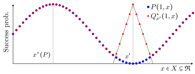
Figure 1: Worst-case deceitful reward distribution $Q^{\star}_{x^{\prime}}$ for a deceitful arm $x^{\prime}$ in a Bernoulli Lipschitz bandit with reward distribution $P$ and optimal arm $x^{\star}(P)$. Here we let $d(x,x^{\prime})=\abs{x-x^{\prime}}$.

5 High-Level Ideas of Our Policy

Our policy, which is called DUal Structure-based Algorithm (DUSA), is inspired by the lower bound formulation discussed in the previous section. The lower bound problem (5) suggests that to obtain minimal regret, each suboptimal arm $x$ in $\tilde{X}(\optp)$ should be explored at least $N_{t+1}(x)=\eta_{\epsilon}(x,\optp)\cdot\log(t)$ times. The logarithmic exploration rate $\eta_{\epsilon}(P)$ is an arbitrary $0<\epsilon$-suboptimal solution, i.e., $\eta_{\epsilon}(P)$ is a feasible solution to problem (5) and achieves an objective value at most $\epsilon$ worse than $C(\optp)$, instead of an actual minimizer. We consider near optimal solutions to circumvent the technical difficulty that the infimum in (5) may not be attained. We discuss later that considering such near optimal exploration rates $\eta_{\epsilon}(P)$ is desirable even if actual minimizers do exist.

Following the previously discussed strategy is evidently not possible without knowing the true reward distribution $\optp$. Our idea is to keep track of the reward distribution of each arm with the help of the empirical counterpart $P_{t}$ constructed based on the historical rewards observed before round $t$. The policy then ensures that the number of times each arm $x$ is pulled during the first $t$ rounds, which is denoted by $N_{t+1}(x)$, is close to $\eta_{\epsilon}(x,P_{t})\cdot\log(t)$ where the logarithmic rate $\eta_{\epsilon}(P_{t})$ is an $0<\epsilon$-suboptimal solution of the following optimization problem

$$\begin{split}C(P_{t})=\inf_{\eta}&~{}\textstyle\sum_{x\in\tilde{X}(P_{t})}\eta(x)\Delta(x,P_{t})\\ \st&~{}\eta\geq 0,~{}1\leq\dis(\eta,x,P_{t})~{}~{}\forall x\in\xd(P_{t}).\end{split}$$ (16)

In the following, we first discuss why and when mimicking the regret lower bound leads to a good learning policy. This discussion leads to a mild assumption on the true reward distribution $P$. Afterward, we argue that in general mimicking the regret lower bound, i.e., solving the semi-infinite problem (16), is computationally expensive. Motivated by this, we present a computationally-efficient convex dual-based approach instead.

5.1 When/Why Mimicking the Lower Bound Works

The proposed strategy aims to play suboptimal arms at the logarithmic target rate $\eta_{\epsilon}(P_{t})$ in any round $t$. Such a strategy can attain asymptotic optimality when by converging the empirical distribution $P_{t}$ to the true reward distribution $P$, (i) the empirical counterpart of the regret lower bound, i.e., $C(P_{t})$, approaches the actual regret lower bound, i.e., $C(P)$, and (ii) the empirical (suboptimal) logarithmic target rate $\eta_{\epsilon}(P_{t})$ converges to $\eta_{\epsilon}(P)$. To meet these requirements, at the reward distribution $P$, the regret lower bound function $C(Q)$ should be continuous and the $\epsilon$-suboptimal exploration rates $\eta_{\epsilon}(Q)$ should admit a continuous selection at $P$. We note that $\eta_{\epsilon}(Q)$ may be a set-valued mapping and as a result, it is necessary to design a selection rule that chooses one of the suboptimal solutions while ensuring that the designed rule is continuous in the reward distribution.

The non-uniqueness of $\epsilon$-suboptimal solutions, although at first glance perhaps perceived as an undesirable complication, is in fact a blessing in disguise. It indeed enables the existence of a continuous selection and echos our previous point that considering $\epsilon$-suboptimal solutions is beneficial as the exact minimizers $\eta^{\star}(Q)$ (should they exist) may fail to admit such continuous selection.

Example 4 (Continued)

1. Lipschitz Bernoulli bandits. We have previously determined $\eta^{\star}(Q)$ in the context of Bernoulli Lipschitz Bandits as the minimizers in the parametric linear optimization problems stated in Equation (15). However, it is well known (Bank et al. 1982, Section 4.3) that the minimizers in such parametric linear optimization problems are upper semi-continuous but not necessarily lower semi-continuous mappings. In Figure 2(a), we attempt to illustrate the lack of continuous exploration rate selections from such upper semi-continuous mappings $\eta^{\star}(Q)$. In this figure, at the reward distribution $P$, the optimal exploration rate $\eta$ is not unique and can be any point in a vertical line. The illustrated optimal mapping $\eta^{\star}(Q)$ is upper semi-continuous, but not lower semi-continuous. For this mapping, one cannot choose one of the optimal solutions at $P$ that leads to a continuous selection. However, this figure shows that this problem is alleviated by considering an $\epsilon$-suboptimal mapping instead. Here, the green area illustrates all the $\epsilon$-suboptimal solutions ($\eta_{\epsilon}(Q)$) and the red curve ($\eta^{\prime}_{\epsilon}(Q)$) presents a particular continuous selection for the $\epsilon$-suboptimal mapping.

The following mild assumption on the reward distribution $P$ is necessary to guarantee the necessary continuity properties.

Assumption 1

The reward distribution $P$

1. has a unique optimal arm,

2. satisfies $\rew_{\max}(x,P)\neq\rew^{\star}(P)$ for any $x\in X$, and

3. is in the interior of $\mathcal{P}$.

Here, $\rew_{\max}(x,P)$ is defined in Equation (9) and $\rew^{\star}(P)=\sum_{r\in\setr}rP(r,x^{\star}(\optp))$. Let $\mathcal{P}^{\prime}\subseteq\mathcal{P}$ denote the set of all such distributions.

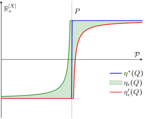
(a)

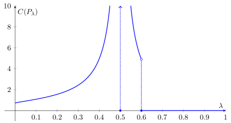
(b)

Figure 2: (a) The mapping $\eta^{\star}(Q)$ between a reward distribution $Q$ and the set of all optimal exploration rates is typically merely upper semi-continuous but not necessarily lower semi-continuous. Even though the optimal exploration rates may exist, there exists no continuous selection at the reward distribution $P$ where the optimal exploration rates are not uniquely defined. Considering $\epsilon$-suboptimal solutions for $\epsilon>0$ alleviates this problem. (b) The regret lower bound $C(P_{\lambda})$ for the separable bandit problem discussed in Section 5.1.

The first condition in Assumption 1 requires the optimal arm under the true reward distribution to be unique. The second condition, i.e., $\rew_{\max}(x,P)\neq\rew^{\star}(P)$ for any $x\in X$, implies that there exists a neighborhood around the true reward distribution $P$ such that for any distribution $Q$ within this neighborhood, the sets of deceitful arms $\xd(Q)$, non-deceitful arms $\xn(Q)$, and optimal arm $x^{\star}(Q)$ are the same. Recall that the suboptimal arm $x\in\xd(P)$ if $\rew_{\max}(x,P)>\rew^{\star}(P)$ and the suboptimal arm $x\in\xd(P)$ if $\rew_{\max}(x,P)\leq\rew^{\star}(P)$. As we show at the end of this section via counter example, both of these conditions are essential for the regret lower bound $C(P)$ as well its (suboptimal) solutions $\eta_{\epsilon}(P)$ to be continuous. The last assumption that $P\in\interior(\mathcal{P})$ ensures that our estimator $P_{t}$ eventually realizes in the set of all potential reward distributions $\mathcal{P}$. That is, we have asymptotically $\lim_{t\to\infty}\Prob{P_{t}\in\mathcal{P}}=1$. We believe that this last assumption is not critical in that is tied to the naive empirical estimator $P_{t}$ that does not exploit the structural information. As a more sophisticated estimator would make the regret analysis of our policy far more complicated, we do not explore this approach in this work and leave it as a future direction.

Proposition 3 (Continuity of Regret Lower Bound)

Consider the regret lower bound problem (5) characterizing the regret lower bound function. Recall that $\mathcal{P}^{\prime}\subseteq\mathcal{P}$ is the set of all distributions that satisfy Assumption 1. Then,

1. the regret lower bound function $C(Q)$ is continuous on $\mathcal{P}^{\prime}$, and

2. there exists an $0<\epsilon$-suboptimal rate selection $\eta^{c}_{\epsilon}(Q)$ which is continuous on $\mathcal{P}^{\prime}$.

The proof of this result, along with other continuity results, is presented in Appendix LABEL:sec:Continuity. We now argue that the first two conditions in Assumption 1 are necessary by considering a simple example. Consider a separable Bernoulli bandit problem with only two arms $X=\{a,b\}$. The reward distribution of the first arm $a$ is such that $P(0,a)\geq\frac{2}{5}$ and the reward distribution of the second arm $b$ can be arbitrary. That is, $\mathcal{P}$ is given in Equation (10). For any $\lambda\in[0,1]$, we define parameterized reward distributions $P_{\lambda}(a)=[\frac{1}{2},\frac{1}{2}]$ and $P_{\lambda}(b)=[1-\lambda,\lambda]$. That is, the probability of receiving reward zero under arm $a$ (respectively arm $b$) is $\frac{1}{2}$ (respectively $1-\lambda$). Then, it is easy to see that the optimal arms and reward are given by

$$x^{\star}(P_{\lambda})=\begin{cases}\{b\}&{\mathrm{if}~{}}\lambda\in(\frac{1}{2},1],\\ \{a,b\}&{\mathrm{if}~{}}\lambda=\frac{1}{2},\\ \{a\}&{\mathrm{if}~{}}\lambda\in[0,\frac{1}{2})\end{cases}\hskip 20.00003pt{\mathrm{and}}\hskip 20.00003pt\rew^{\star}(P_{\lambda})=\begin{cases}\lambda&{\mathrm{if}~{}}\lambda\in(\frac{1}{2},1],\\ \frac{1}{2}&{\mathrm{if}~{}}\lambda\in[0,\frac{1}{2}].\end{cases}$$

Observe that at $\lambda=\frac{1}{2}$, the optimal arm is not unique. That is, the first condition of Assumption 1 is violated. Furthermore, at $\lambda=\frac{3}{5}$, we have $\rew_{\max}(a,P)=\rew^{\star}(P)$. That is, the second condition of Assumption 1 is violated. Next, we show that these violations result in discontinuity of the regret lower bound.

For the parameter values $\lambda\in[\frac{3}{5},1]$, we have that $\rew^{\star}(P_{\lambda})\geq\rew_{\max}(a,P_{\lambda})=\frac{3}{5}$ and hence $C(P_{\lambda})=0$. Likewise, when $\lambda=\frac{1}{2}$, both arms are optimal, and once again we have that $C(P_{\lambda})=0$. It can be verified that

$$C(P_{\lambda})=\begin{cases}0&{\mathrm{if}}~{}\lambda\in[\frac{3}{5},1]\bigcup\{\frac{1}{2}\},\\ \frac{\lambda-\frac{1}{2}}{\frac{1}{2}\log(\frac{1/2}{\lambda})+\frac{1}{2}\log(\frac{1/2}{1-\lambda})}&{\mathrm{if}}~{}\lambda\in(1/2,\frac{3}{5}),\\ \frac{1/2-\lambda}{\lambda\log(\frac{\lambda}{1/2})+(1-\lambda)\log(\frac{1-\lambda}{1/2})}&{\mathrm{if}~{}}\lambda\in[0,1/2)\,,\end{cases}$$

which we have visualized in Figure 2(b). The function $C(P_{\lambda})$ is evidently discontinuous at parameter value $\lambda$ of $\frac{1}{2}$ and $\frac{3}{5}$, as claimed.

5.2 Dual-based Representation of Regret Lower Bound

To follow the proposed strategy, we may potentially need to solve the regret lower bound problem, i.e., problem (16), in each round. Observe that this optimization problem is a semi-infinite minimization problem, which cannot in general be solved directly. Even verifying the feasibility of a fixed exploration rate $\eta$ requires the solution to the auxiliary information minimization problem (6) defining our information distance function $\dis(\eta,x,P_{t})$. We will overcome this challenge by using an equivalent dual representation of this distance function instead. This novel equivalent dual representation enables us to reformulate the regret lower bound problem (5) and its empirical counterpart problem (16) as standard finite convex minimization problems, which are computationally much more attractive compared to solving their semi-infinite representations directly.

We start with stating an equivalent formulation of the distance function with the help of conic hull of the feasible set $\mathcal{P}$. Let us denote the conic hull of $\mathcal{P}$ as the set $\mathcal{K}=\cone(\mathcal{P})\defn\tset{\theta\cdot Q\!}{\!\theta\geq 0,~{}Q\in\mathcal{P}}\,.$ Observe that this convex cone represents the same information as the set of reward distributions $\mathcal{P}$ as we have the following equivalence: $\mathcal{P}=\tset{Q\!\!}{\!\!\textstyle\sum_{x\in X,r\in\setr}Q(r,x)=\abs{X}}\bigcap\mathcal{K}.$ Working with the cone $\mathcal{K}$ instead of the set $\mathcal{P}$ helps us provide a unified dual formulation later on. This conic representation, along with Proposition 2, allows us to rewrite the information distance function for any deceitful arm $x^{\prime}\in\xd(P)$ as the following minimization problem

$$\begin{array}[]{rl@{\hspace{4em}}l}\dis(\eta,x^{\prime},P)=\min_{Q}&\lx@intercol\sum_{x\in\tilde{X}(P)}\eta(x)I(P(x),Q(x))+\chi_{\infty}(P(x^{\star}(P))=Q(x^{\star}(P)))\hfil\lx@intercol\\[3.00003pt] \st&Q\in\mathcal{K},\hfil\hskip 40.00006pt&[{\mathrm{dual~{}variable:~{}}}\lambda\in\mathcal{K}^{\star}]\\[3.00003pt] &\sum_{x\in X,\,r\in\setr}Q(r,x)=\abs{X},\hfil\hskip 40.00006pt&[{\mathrm{dual~{}variable:~{}}}\beta\in\real]\\[3.00003pt] &\sum_{r\in\setr}rQ(r,x^{\prime})\geq\rew^{\star}(P),\hfil\hskip 40.00006pt&[{\mathrm{dual~{}variable:~{}}}\alpha\in\real_{+}]\end{array}$$ (21)

where $\chi_{\infty}(A)=0$ if event $A$ occurs; $+\infty$ otherwise. Note that in problem (21), all the nonlinear constraints in the minimization problem (6) are captured by the conic constraint $Q\in\mathcal{K}$. We denote with $\lambda$ the dual variable of the cone constraint, $\beta\in\real$. Further, $\alpha\in\real_{+}$ are the dual variables of the second and third constraints, respectively. Let the dual cone $\mathcal{K}^{\star}$ be defined as the unique cone that satisfies $Q\in\mathcal{K}$ if and only if $\iprod{\lambda}{Q}\geq 0,~{}\forall\lambda\in\mathcal{K}^{\star}$, where we take as inner product $\iprod{\lambda}{Q}=\sum_{x\in X,\,r\in\setr}\lambda(r,x)Q(r,x)$. Just as the cone $\mathcal{K}$ captures the same information as the set of reward distributions $\mathcal{P}$, so does its dual cone $\mathcal{K}^{\star}$. This is so because for any closed convex cones, we have $\mathcal{K}^{\star\star}=\mathcal{K}$; see Boyd and Vandenberghe (2004, Section 2.6.1).

For any reward distribution $\optp\in{\mathcal{P}}$ and suboptimal arm $x^{\prime}\in\tilde{X}(\optp)$, we now define our concave dual function:

$$\begin{split}\dual&(\eta,x^{\prime},\optp~{};~{}\mu)\defn\sum_{x\in\tilde{X}(P),r\in\setr}{\textstyle\eta(x)\log\left(\frac{\eta(x)-\lambda(r,x)-\beta-\alpha r\mb 1(x=x^{\prime})}{\eta(x)}\right)\optp(r,x)}-\sum_{x\in x^{\star}(\optp),r\in\setr}\lambda(r,x)\optp(r,x)\\ &+\alpha\rew^{\star}(\optp)+\beta|\tilde{X}(\optp)|+\chi_{-\infty}(\eta(x)-\lambda(r,x)-\beta-\alpha r\mb 1(x=x^{\prime})\geq 0)\,.\end{split}$$ (22)

For notational convenience, we collect all our dual variables in the dual vector $\mu\defn(\alpha,\beta,\lambda)\in\real_{+}\times\real\times\mathcal{K}^{\star}$. Here, the concave characteristic function $\chi_{-\infty}(A)$ takes on the value zero when event $A$ happens; $-\infty$ otherwise. The following lemma characterizes the dual of the distance function $\dis$ using the $\dual$ function defined above.

Lemma 1 (Dual Formulation of the Distance Function)

For any reward distribution $P\in\mathcal{P}_{\Omega}$ and arm $x^{\prime}\in X$, the following weak duality inequality $\dual(\eta,x^{\prime},P~{};~{}\mu)\leq\dis(\eta,x^{\prime},P)$ holds, where $\mu\in\real_{+}\times\real\times\mathcal{K}^{\star}$ is any feasible dual vector to problem (21), the dual function $\dual$ and distance function $\dis$ are defined in Equations (22) and (6), respectively. Furthermore, for any reward distribution $\optp\in\mathcal{P}$ and suboptimal deceitful arm $x^{\prime}\in\xd(\optp)$, the following strong duality equality holds

$$\textstyle\dis(\eta,x^{\prime},\optp)=\sup_{\mu}\set{\dual(\eta,x^{\prime},\optp~{};~{}\mu)}{\mu\in\real_{+}\times\real\times\mathcal{K}^{\star}}.$$ (23)

In the following theorem, we characterize the regret lower bound function using the dual formulation in Lemma 1. The proof of this lemma is presented in Appendix 11.1. Note that all the duality results are presented in Appendix 11.

Theorem 2 (Regret Lower Bound – Dual Formulation)

Consider any reward distribution $\optp\in\mathcal{P}$. The regret lower bound presented in Proposition 1 is characterized equivalently as

$$\begin{array}[]{rl@{\hspace{2em}}l}C(\optp)=\inf_{\eta\geq 0,\,\mu}&\sum_{x\in\tilde{X}(\optp)}\eta(x)\Delta(x,\optp)\hfil\hskip 20.00003pt&\\[5.0pt] \st&\mu(x)\in\real_{+}\times\real\times\mathcal{K}^{\star}\hfil\hskip 20.00003pt&x\in X,\\[5.0pt] &1\leq\dual(\eta,x,\optp~{};~{}\mu(x))\hfil\hskip 20.00003pt&x\in\xd(P).\end{array}$$ (27)

Observe that the dual characterization of the regret lower bound is convex and finite dimensional. We further highlight that the dual problem (27), unlike its primal counterpart (5), is no longer a nested optimization. The complexity and computational issues of solving the dual lower bound representation are discussed in Appendix LABEL:sec:complexity.

6 Dual Structure Algorithm (DUSA)

In this section, we present our policy, called DUSA; see Algorithm 1. The DUSA algorithm is parameterized by a positive number $\epsilon>0$ which we shall refer to as the accuracy parameter. Our optimal algorithm is best understood by considering its asymptotic limit $\epsilon\to 0$. Hence, most of our commentary regarding the intuition behind the algorithm will focus on this regime.

Input. Accuracy parameter $0<\epsilon$.

• Initialization.

  • During the first $|X|$ rounds, pull each arm $x\in X$ once and set $P_{\abs{X}+1}(R(x),x)=1$, where $R(x)$ is the observed reward of arm $x$ in its corresponding round.

  • Let $s_{\abs{X}+1}=0$ and $N_{\abs{X}+1}(x)=1$ for all $x\in X$. For all arms $x\in X$, initialize the dual variables $\lambda_{|X|+1}(x)\in\mathcal{K}^{\star}$, $\alpha_{|X|+1}(x)\in\real_{+}$, and $\beta_{|X|+1}(x)\in\real$ and reference logarithmic rate $\eta_{|X|+1}^{\prime}(x)>0$.

• For $t\in\abs{X}+1,\dots$

  • Sufficient information condition. For every deceitful arm $x\in\xd(P_{t})$, solve the following convex univariate minimization problem $\overline{\dual}_{t}(x)\defn\overline{\dual}\left(\tfrac{N_{t}}{\log(t)},x,P_{t}~{};~{}\mu_{t}(x)\right)\defn{\displaystyle\max_{\rho\geq 0}}~{}\dual\left(\tfrac{N_{t}}{\log(t)},x,P_{t}~{};~{}\rho\mu_{t}(x)\right).$

  • Exploitation. If $\overline{\dual}_{t}(x)\geq 1+\epsilon$ for all deceitful arms $x\in\xd(P_{t})$, then $s_{t+1}=s_{t}$, $\mu_{t+1}=\mu_{t}$, $\eta^{\prime}_{t+1}=\eta^{\prime}_{t}$ and pull a least played empirically optimal arm $x_{t}\in\textstyle\arg\min\set{N_{t}(x^{\prime})}{x^{\prime}\in\arg\max_{x\in X}\sum_{r\in\setr}rP_{t}(r,x)}.$

  • Exploration. Else, set $s_{t+1}=s_{t}+1$. Furthermore,

    • If $\min_{x\in X}N_{t}(x)\leq{\color[rgb]{0,0,0}\frac{\epsilon s_{t}}{1+\log(1+s_{t})}}$, pull the least pulled arm $x_{t}=\underline{x}_{t}\in\arg\min_{x\in X}N_{t}(x)\,.$

    • Update exploration target rates $\eta_{t}=\text{\sf SU}(P_{t},\eta^{\prime}_{t}~{};~{}\mu_{t},\epsilon)$ using shallow update Algorithm 6 and let $\bar{x}_{t}\in\textstyle\arg\min_{x\in X}\tfrac{N_{t}(x)}{\eta_{t}(x)}.$

    • Let $x_{t}^{\star}\in\textstyle\arg\min\set{N_{t}(x^{\prime})}{x^{\prime}\in X^{\star}_{t}}$ be the empirically optimal arm. If $N_{t}(x^{\star}_{t})\leq N_{t}(\bar{x}_{t})$, pull $x_{t}=x_{t}^{\star}.$ Else, pull $x_{t}=\bar{x}_{t}.$

    • Update dual variables $(\eta^{\prime}_{t+1},\mu_{t+1})=\text{\sf DU}(P_{t}~{};~{}\epsilon)$ using deep update Algorithm 3.

  • Updating variables.

    • Observe reward of the pulled arm $R_{t}(x_{t})$. For any $x\in X$, $x\neq x_{t}$, and $r\in\setr$, set $P_{t+1}(r,x)=P_{t}(r,x)$. Further, for any $r\neq R_{t}(x_{t})$, $P_{t+1}(r,x_{t})=N_{t}(x_{t})P_{t}(r,x_{t})/(N_{t}(x_{t})+1)$, and $P_{t+1}(R_{t}(x_{t}),x_{t})=\big{(}1+N_{t}(x_{t})P_{t}(R_{t}(x_{t}),x_{t})\big{)}/(N_{t}(x_{t})+1)$. Set $N_{t+1}(x_{t})=N_{t}(x_{t})+1$ and for any $x\neq x_{t}$, $N_{t+1}(x)=N_{t}(x)$.

Algorithm 1 DUal Structure Algorithm (DUSA)

Initialization phase. DUSA starts with an initialization phase of $|X|$ rounds. During these first $|X|$ rounds, it pulls each arm $x\in X$ once. Then, based on the observed rewards in these rounds, it initializes its estimate for the reward distribution. As before, the estimate $P_{t}$ is the empirical distribution of the observed rewards before round $t$. At the end of the initialization phase, i.e., round $t=|X|$, DUSA initializes the dual variables for each arm $x$, i.e., $\alpha_{t+1}(x)$, $\beta_{t+1}(x)$, and $\lambda_{t+1}(x)$, and the reference logarithmic rate, denoted by $\eta^{\prime}_{t+1}(x)$.

Sufficient information and resolving test. After the initialization phase, DUSA aims to strike a balance between exploration and exploitation. To do so, it checks if for any empirically deceitful arm $x\in\xd(P_{t})$, the following sufficient information condition holds:

$$1+\epsilon\leq\!\overline{\dual}_{t}(x)\defn\!\textstyle\overline{\dual}\left(\frac{N_{t}}{\log(t)},x,P_{t}~{};~{}\mu_{t}(x)\right):={\displaystyle\max_{\rho\geq 0}}~{}\textstyle{\dual}\left(\frac{N_{t}}{\log(t)},x,P_{t}~{};~{}\rho\cdot\mu_{t}(x)\right).$$ (28)

Here, $\mu_{t}(x)=(\alpha_{t}(x),\beta_{t}(x),\lambda_{t}(x))$ are the dual variables for arm $x$ employed in round $t$. Remark that verifying the sufficient information condition merely requires the resolution of a univariate convex optimization problem. ( See Section 7 for computation time of this simple univariate convex optimization problem in various structured bandits.) We refer to previously defined function $\overline{\dual}$ as the dual-test function. Roughly speaking, our condition verifies whether sufficient information has been collected to distinguish the empirical $P_{t}$ from its deceitful distributions; that is, whether or not $\dis(\tfrac{N_{t}}{\log(t)},x^{\prime},P_{t})\geq\overline{\dual}\left(\tfrac{N_{t}}{\log(t)},x^{\prime},P_{t}~{};~{}\mu_{t}\right)\geq 1+\epsilon$ for any $x^{\prime}\in\tilde{X}(P_{t})$. In Appendix 11.3, we provide a further clarifying interpretation of this sufficient information test as the information distance between $P_{t}$ and a half-space containing all deceitful distributions $\prob(x^{\prime},P)$. As we will show later, our sufficient information condition helps DUSA solve the lower bound problem (27) only in $\mc O(\log(T))$ rounds.

Exploitation. If the sufficient information condition holds for all deceitful arms $x\in\xd(P_{t})$, DUSA enters an exploitation phase and it selects a least played empirically optimal arm, i.e., $x_{t}\in\textstyle\arg\min\set{N_{t}(x^{\prime})}{x^{\prime}\in X_{t}^{*}},$ where $X_{t}^{\star}=\arg\max_{x\in X}\sum_{r\in\setr}rP_{t}(r,x)$.

Exploration. If the sufficient information test fails, DUSA enters an exploration phase as insufficient information has been collected on the empirically suboptimal arms $\tilde{X}(P_{t})$ in the previous rounds. Let $s_{t}$ be the number of exploration rounds in the first $t-1$ rounds. Then, if $\min_{x\in X}N_{t}(x)\leq{\color[rgb]{0,0,0}\epsilon\tfrac{s_{t}}{(1+\log(1+s_{t}))}}$, DUSA pulls the least pulled arm $\underline{x}_{t}$. Otherwise, it considers a new $2\epsilon$-suboptimal logarithmic target rate $\eta_{t}$ in

$$\begin{array}[]{rl}\overline{C}(P_{t}~{};~{}\mu_{t}):=\inf_{\eta\geq 0}&\sum_{x\in\tilde{X}(P_{t})}\eta(x)\Delta(x,P_{t})\\[5.0pt] \st&1\leq\overline{\dual}(\eta,x,{P_{t}};~{}\mu_{t}(x))\quad\forall x\in\xd({P_{t}}).\end{array}$$ (31)

This infimum can be computed efficiently because it is characterized as the minimum of a linear objective over an ordinary convex optimization constraint set. However, as $2\epsilon$-suboptimal solutions are not unique, a particular selection must be made. To do so, the shallow update (SU) Algorithm 6 selects the exploration rate closest to some reference logarithmic rate $\eta^{\prime}_{t}$. As the optimization characterization (35) is strictly convex, its minimizer when feasible must be unique. Our selection procedure thus circumvents the potential pitfall that the infimum (31) may not in fact admit a minimizer and as outlined in Proposition 5 enjoys much better continuity properties even if this infimum is in fact attained.

Let $\eta_{t}=\text{\sf SU}(P_{t},\eta^{\prime}_{t}~{};~{}\mu_{t},\epsilon)$ be the output of the shallow update Algorithm and define $\bar{x}_{t}\in\textstyle\arg\min_{x\in X}\tfrac{N_{t}(x)}{\eta_{t}(x)}$. When $N_{t}(x^{\star}_{t})\leq N_{t}(\bar{x}_{t})$, the algorithm plays the empirically optimal arm $x^{\star}_{t}\in\textstyle\arg\min\set{N_{t}(x^{\prime})}{x^{\prime}\in X^{\star}_{t}}$. Otherwise, DUSA pulls a suboptimal arm $\bar{x}_{t}\in\textstyle\arg\min_{x\in\tilde{X}(P_{t})}\tfrac{N_{t}(x)}{\eta_{t}(x)}$ whose empirical logarithmic exploration rate deviates from its optimal target rate to the largest relative extent. The condition $N_{t}(x^{\star}_{t})\leq N_{t}(\bar{x}_{t})$ signals that empirically optimal arm $x_{t}^{\star}$ has not been sufficiently explored to justify the forced exploration of $\bar{x}_{t}$. Hence, when $N_{t}(x^{\star}_{t})\leq N_{t}(\bar{x}_{t})$, $x^{\star}_{t}$ is pulled instead of $\bar{x}_{t}$ to ensure $x^{\star}_{t}$ is explored enough.

Input. Reward distribution $Q$, reference exploration target rate $\eta^{\prime}$, dual variable $\mu=(\alpha,\beta,\lambda)$, and accuracy parameter $\epsilon>0$. Compute

Algorithm 2 Shallow Update $\text{\sf SU}(Q,\eta^{\prime}~{};~{}\mu,\epsilon)$

$$\begin{array}[]{rl}\eta_{\epsilon}(Q)\defn\arg\min_{\eta\geq 0}&\sum_{x\in X}(\eta(x)-\eta^{\prime}(x))^{2}\\[5.0pt] \st&1\leq\overline{\dual}(\eta,x,Q~{};~{}\mu(x))\quad\forall x\in\xd(Q),\\[5.0pt] &\sum_{x\in\tilde{X}(Q)}\eta(x)\Delta(x,Q)\leq\overline{C}(Q~{};~{}\mu)+2\epsilon.\end{array}$$ (35)

If no feasible solution exists, we simply set $\eta_{\epsilon}(Q)\defn+\infty$. Return. $\eta_{\epsilon}(Q)$.

Finally, DUSA updates the reference rate $\eta^{\prime}_{t}$ and dual variables $(\eta^{\prime}_{t},\mu_{t})=\mathrm{DU}(P_{t},\epsilon)$ using the deep update (DU) Algorithm 3. The deep update algorithm returns a $\epsilon$-suboptimal solution of the dual counterpart of the lower bound problem (27) computed at the empirical reward distribution $P_{t}$. As the dual counterpart of the lower bound problem (27) is an convex optimization problem, such $\epsilon$-suboptimal solutions can be readily determined. However, for reasons discussed previously, these solutions are not unique and a particular selection must be made. Our deep update algorithm selects a certain minimal norm solution over a slightly restricted feasible set. As the optimization formulation (42) in the deep update algorithm is strictly convex, its minimizer is always unique. Note that the first and second sets of constraints in problem (42) are the same as those in problem (27). This ensures that any feasible solution to problem (42) is a feasible solution to problem (27). The third set of constraints of problem (42) guarantees any feasible solution to this problem to be an $\epsilon$-suboptimal solution to problem (27). Note that the optimal value $C(Q)$, which appears in the third constraint, can be obtained simply by solving an ordinary convex optimization problem. The fourth set of constraints of problem (42) ensures $\eta$ to be bounded away from zero and helps us establish continuity of the optimal solution to problem (42). The last set of constraints of this problem guarantees the dual function $\dual$ to be finite. We would like to stress that, thanks to our sufficient information test, we do not carry out either the deep or shallow update in every round.

Input. Reward distribution $Q$ and accuracy parameter $\epsilon>0$. Let $\eta_{\epsilon}^{\prime}(Q),\mu_{\epsilon}(Q))$ be

$$\begin{array}[]{r@{~~}l}\arg{\displaystyle\min_{\eta,\mu}}~{}~{}&\sum_{x\in X}\eta(x)^{2}+\sum_{x\in X}\norm{\mu(x)}_{2}^{2}\\[5.0pt] \st~{}~{}&\eta(x)\in\real_{+},~{}\mu(x)=(\alpha(x),\beta(x),\lambda(x))\in\mathcal{K}^{\star}\times\!\real_{+}\!\times\!\real~{}~{}\forall x\in X,\\[5.0pt] ~{}~{}&1\leq\dual(\eta,x,Q~{};~{}\mu(x))\quad\forall x\in\xd(Q),\\[5.0pt] ~{}~{}&\sum_{x\in\tilde{X}(Q)}\eta(x)\Delta(x,Q)\leq C(Q)+\epsilon,\\[5.0pt] ~{}~{}&\eta(x)\geq\epsilon/(2\sum_{x\in\tilde{X}(Q)}\Delta(x,Q))\quad\forall x\in\tilde{X}(Q),\\[5.0pt] ~{}~{}&\eta(x)\geq\lambda(r,x)(x^{\prime})\!+\!\beta(x^{\prime})\!+\!\alpha(x^{\prime})r\mb 1(x=x^{\prime})\!+\!\frac{\epsilon}{(2\sum_{x\in\tilde{X}(Q)}\Delta(x,Q))}~{}\forall x^{\prime}\in\xd(Q),\,x\in\tilde{X}(Q).\end{array}$$ (42)

Return. $(\eta_{\epsilon}^{\prime}(Q),\mu_{\epsilon}(Q))$.

Algorithm 3 Deep Update $\textsc{DU}(Q~{};~{}\epsilon)$

As discussed earlier, it is critical to have a continuous selection rule as the $\epsilon$-suboptimal solutions are not unique. The subsequent proposition points out that our deep update selection rule is indeed well-defined and continuous on $\mc P^{\prime}$ as required; see the proof of this result in Appendix LABEL:sec:continuous-selections.

Proposition 4 (Continuous Selection Rule for the Deep Update Algorithm)

Our deep update selection rule $(\eta_{\epsilon}^{\prime}(Q),\mu_{\epsilon}(Q))$, presented in Equation (42), exists and is continuous on $\mathcal{P}^{\prime}$, where $\mathcal{P}^{\prime}$ consists of all the distributions in $\mathcal{P}$ that satisfy Assumption 1.

To establish our main result stated in Theorem 3, we also require the shallow update selection rule to be stable. The shallow update is stable in the sense that $\text{\sf SU}(P_{t},\eta_{\epsilon}^{\prime}(P_{t^{\prime}})~{};~{}\mu_{\epsilon}(P_{t^{\prime}}),\epsilon)$ converges to the desired reference rate $\eta^{\prime}_{\epsilon}(P)$ when both empirical distributions $P_{t}$ and $P_{t^{\prime}}$ approach the true reward distribution $P$. This notion of stability for the shallow update is formalized in the following proposition and will be crucial to establish the optimality of our DUSA policy.

Proposition 5 (Stability of the Shallow Update Selection Rule)

For any $P\in\mathcal{P}^{\prime}$, we have

$$\begin{array}[]{rl@{\quad}l}\lim_{\kappa\to 0}~{}\max_{Q_{1},Q_{2}}&\norm{\text{\sf SU}(Q_{1},\eta_{\epsilon}^{\prime}(Q_{2})~{};~{}\mu_{\epsilon}(Q_{2}),\epsilon)-\eta^{\prime}_{\epsilon}(P)}_{2}&=\quad 0.\\[5.0pt] \st&\norm{Q_{1}-P}_{\infty}\leq\kappa,~{}\norm{Q_{2}-P}_{\infty}\leq\kappa&\end{array}$$

The proof of Proposition 5 is in Appendix LABEL:sec:proof:shallow. We now present our main result.

Theorem 3 (Regret Bound of DUSA)

Let the true reward distribution $P\in\mathcal{P}^{\prime}$ and consider any accuracy parameter $0<\epsilon<\tfrac{1}{\abs{X}}$. Then, DUSA suffers the following asymptotic regret:

$$\limsup_{T\to\infty}\textstyle~{}\frac{\reg(T,\optp)}{\log(T)} \leq\textstyle(1+\epsilon)(C(\optp)+\epsilon\left(1+\sum_{x\in X}\Delta(x,\optp)\right))\,,$$ (45)

where the regret is computed against the benchmark that knows the best arm in advance. Furthermore, the expected number of rounds in which DUSA enters the exploration phase in bounded by

$$\limsup_{T\to\infty}\textstyle~{}\frac{\E{}{s_{T}}}{\log(T)} \leq(1+\epsilon)\abs{X}^{2}(\norm{\eta^{\prime}_{\epsilon}(\optp)}_{\infty}+\epsilon)\,,$$ (46)

where the expectation is taken with respect to the randomness in the observed rewards and choices made by DUSA.

Comparing the regret lower bound in Proposition 1 with the regret upper bound found in Equation (45), we can hence conclude that DUSA enjoys the minimal asymptotic logarithmic regret as the accuracy parameter $\epsilon$ goes to zero. The maximum target exploration rate $\norm{\eta^{\prime}_{\epsilon}(P)}_{\infty}=\max_{x\in\tilde{X}(P)}\eta^{\prime}(x,P)$ appearing in our bound on number of exploration rounds in Equation (46) remains bounded uniformly for all accuracy parameter values $\epsilon>0$. This is so because (i) we have from $\epsilon$-suboptimality that $\textstyle\sum_{x\in\tilde{X}(P)}\eta^{\prime}_{\epsilon}(x,P)\Delta(x,P)\leq C(P)+\epsilon<\infty$, and (ii) $\Delta(x,P)>0$ for all suboptimal arms. Hence, the number of times we have to update the target exploration rates and dual variables using either the shallow or deep update Algorithms 6 and 3 grows merely logarithmically in the number of rounds $T$. Note that the number of updates is equal to the number of the exploration rounds. Theorem 3 does not bound the regret of DUSA for any finite number of rounds but instead is completely asymptotic in nature. Nevertheless, in the proof of Theorem 3, which we will present in Appendix 12, non-asymptotic regret bounds are also derived. The non-asymptotic regret of DUSA can be upper bounded by $C_{\rm{initialize}}+C_{\text{exploit}}+C_{\text{explore}}$, where $C_{\rm{initialize}}=|X|$ and $C_{\text{exploit}}$ defined in Equation (LABEL:eq:c_exploit) are, respectively, upper bounds on the regret during the initialization and exploitation rounds. Interestingly, thanks to our sufficient information test, $C_{\text{exploit}}$ does not contribute to the asymptotic regret. The term $C_{\text{explore}}$, which is the dominating factor in the asymptotic regret, is an upper bound on the regret during the exploration rounds. In the proof of Theorem 3, the term $C_{\text{explore}}=C_{2}+C_{3}+C_{4}$ is itself decomposed into three components. The terms $C_{2}$ (respectively $C_{3}+C_{4}$) is an upper bound on the regret during exploration rounds when the empirical reward distribution is “far from” (respectively “close to”) the true reward distribution.

Remark 1 (Nondeceitful Bandits)

When the bandit $P\in\mc P^{\prime}$ is nondeceitful, i.e., $\tilde{X}_{d}(P)=\emptyset$, the regret lower bound function $C(P)=0$ vanishes which opens up the possibility of achieving a sublogarithmic regret. Jun and Zhang (2020) propose a bandit policy which in fact achieves a bounded regret on such nondeceitful bandits. See also Lattimore and Munos (2014), Gupta et al. (2020) for similar results. We show in Remark LABEL:rem:proof:nondeceitful-bandits in the proof of our main Theorem 3 that the regret of DUSA also remains bounded for all $T$ on such nondeceitful bandits.

7 Numerical Experiments

In this section, we evaluate the performance of DUSA in the context of several structural bandit problems discussed in Section 3.1. We first focus on linear and Lipschitz bandits, which are well-known structured bandits. Then, to illustrate the flexibility of DUSA, we further evaluate DUSA in the context of dispersion bandits. We begin by explaining how DUSA is implemented.

7.1 DUSA Implementation

We have implemented our DUSA bandit policy for the discussed linear, Lipschitz and dispersion bandits discussed in Section 3.1 in Julia. All code is available as a Julia package at https://tinyurl.com/473y3wr5. The code is written in a modular fashion which allows to quickly extend our DUSA package to other structures beyond those we have implemented. Notice that every structured bandit problem is uniquely characterized by a convex set $\mc P$. Extending DUSA to be able to deal with any convex bandit problems is as simple as exposing its associated dual cone $\mc K^{\star}=\cone(\mc P)^{\star}$ to the package; see also Section 5.2. In every exploration round, DUSA may need to compute both the shallow and deep updates stated in Section 6. These updates demand the solution of a convex optimization problem. The resulting exponential cone optimization problems are subsequently solved using the commercial exponential cone interior point solver Mosek.

In our practical implementation, we make two minor changes in DUSA. First, instead of carrying out the shallow and deep updates exactly as stated in Algorithms 6 and 3, we simply return an arbitrary $\epsilon$-suboptimal solution to the optimization problems (31) and (16), respectively. In all numerical results we set our accuracy parameter as $\epsilon=1\e{-3}$. Second, in our implementation, DUSA policy enters the exploitation phase when the following sufficient test passes for all empirically deceitful arms $x\in\xd(P_{t})$: $\overline{\dual}_{t}(x)\geq(1-\exp(-t/T_{0}))\cdot(1+\epsilon)\,,$ where we set $T_{0}=2000$. This information test is slightly different from the one described in Algorithm 1. Our DUSA policy as described in Algorithm 1 only enters the exploitation phase when the sufficient information test $\overline{\dual}_{t}(x)\geq 1+\epsilon$ passes for all empirically deceitful arms $x\in\xd(P_{t})$. We found that replacing this test with this slightly modified version (i.e., $\overline{\dual}_{t}(x)\geq(1-\exp(-t/T_{0}))\cdot(1+\epsilon)$) avoids over-exploration during the early rounds of our policy. Finally, we note that computing $\overline{\dual}_{t}(x)$ for any such arm $x$ merely demands the solution of the univariate convex optimization problem in Equation (28) which we determine with a simple bisection search.

7.2 Evaluating DUSA Under Well-known Structured Bandits

7.2.1 Linear Bandits

Setup. We consider linear bandits with ten arms; that is $|X|=10$. The reward of arm $x\in X$ is drawn from a Bernoulli distribution with the mean $c_{x}^{T}\theta$. Here, $c_{x}$ and $\theta=[\hat{\theta}^{T},1]^{T}$ are 5-dimensional vectors, where $\hat{\theta}$ is a 4-dimensional vector and each element of $\hat{\theta}$ is drawn independently from a standard normal distribution. After generating $\theta$, we generate $c_{x}$. To do so, we first generate a 4-dimensional vector, denoted by $\hat{c}_{x}$, where each element of this vector is drawn from a standard normal distribution. We then set $c_{x}=[a\cdot\hat{c}_{x}^{T},b]^{T}$, where $a,b\in\mathbb{R}$ are chosen such that $\max_{x\in X}c_{x}^{T}\theta=0.9$ and $\min_{x\in X}c_{x}^{T}\theta=0.1$. We consider $120$ problem instances, where each problem instance corresponds to a particular coefficient vector $\theta$ and $(c_{x})_{x\in X}$. For each problem instance, we run our DUSA algorithm and the GLM-UCB algorithm of Filippi et al. (2010) $20$ times over $T=5,000$ rounds. Linear bandit problems are a special case of the parametric bandits discussed in Section 3.1 and are explicitly characterized by $\mc P_{\rm{lin}}=\set{Q\in\mc P_{\Omega}}{\forall x\in X,~{}\exists\theta~{}\st~{}\textstyle\sum_{r\in\setr}rQ(r,x)=c_{x}^{T}\theta}.$ Our DUSA algorithm can specialized to this class of convex bandit problems simply by considering the associated dual cone $\mc K_{\rm lin}^{\star}=\cone(\mc P_{\rm lin})^{\star}$ explicitly characterized in Appendix 11.5.

The GLM-UCB algorithm of Filippi et al. (2010), which uses an upper confidence bound principle, needs to solve two optimization problems in every round; see Equations (6) and (7) in Filippi et al. (2010). The first optimization problem, which is a maximum likelihood estimation step for $\theta$, is convex problem and is easy to solve. The second problem—which involves a projection step for the estimated value of $\theta$ obtained from the maximum likelihood estimation approach—is quite complex to solve. To implement GLM-UCB, we only solve the first optimization problem. However, to ensure that we do not return solutions which are too far from the true value $\theta$, we provide upper and lower bounds on the values that $\theta$ may take in the first optimization problem. Despite this change, the GLM-UCB policy remains very slow. To make it faster, we only solve the first optimization problem every $200$ rounds. Finally, we choose the confidence parameter of GLM-UCB as $\rho(t)=\sqrt{\tfrac{0.3}{\log(t)}}$ where the constant $0.3$ is chosen using cross validation.

Figure 3(a) depicts the normalized cumulative regret of DUSA and GLM-UCB as a function of the number of rounds. Here, the normalized cumulative regret is the ratio of the cumulative regret over $T$ rounds to the asymptotic regret lower bound $C(P)\log(T)$ as in Proposition 1. Each of these box plots depict $2,400$ data points as we generate $120$ problem instances and we run each problem instance $20$ times. We observe that the median of the normalized cumulative regret of DUSA and GLM-UCB are comparable. However, the normalized cumulative regret of DUSA is more concentrated around its median than that of GLM-UCB. For instance, for GLM-UCB, we observe an outlier whose cumulative regret is around $20$ times the regret lower bound. On the other hand, the worst cumulative regret experienced by DUSA is less than $7$ times the regret lower bound, which suggests that DUSA is more reliable than GLM-UCB when it comes to worst-case performance. See Appendix 9 for similar experiments with $\abs{X}=5$ and $\abs{X}=15$.

We now comment on computation time of DUSA. The computational time of DUSA is primarily determined by how fast the deep update in Algorithm 3 can be carried out. Crucially, the deep update is only carried out in some of exploration rounds. The average computation time to carry out exploration rounds is here $0.3$ seconds while the average computation time for exploitation rounds is considerably less at $0.06$ seconds. Finally, the overall average computation time per round measured $0.09$ seconds indicating that, as expected, the number of exploitation rounds makes up a large fraction of all $T$ rounds.

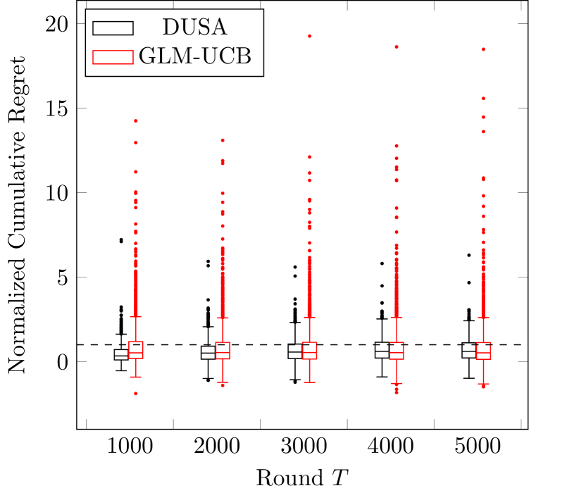
(a) Linear Bandits

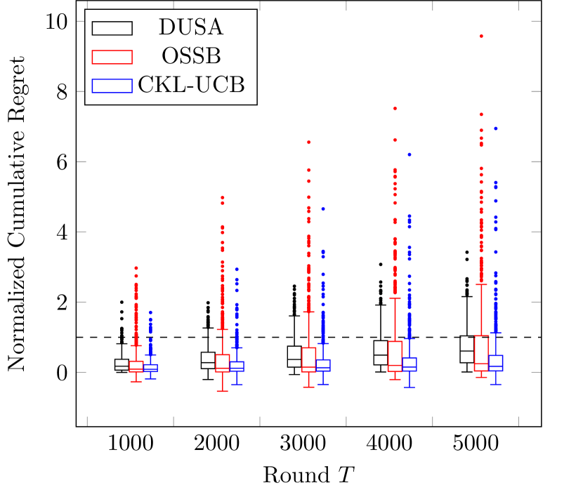
(b) Lipschitz Bandits

Figure 3: The normalized cumulative regret of DUSA on linear and Lipschitz bandit instances as a function of the number of rounds $T$.

7.2.2 Lipschitz Bandits

Setup. We consider Lipschitz bandits with $10$ arms and Lipschitz constant $L=0.5$. The reward of each arm $x$ is drawn from a Bernoulli distribution with mean $\theta(x)$. Here, we use the same setup as in Magureanu et al. (2014) and set $\theta(x)=0.8-0.5\cdot|0.5-x|$, where $x$ is drawn from the uniform distribution on the interval $[0,1]$. We consider $150$ problem instances where we run each problem instance $5$ times over the course of $T=5,000$ rounds. Recall that Lipschitz bandit problems as discussed in Section 3.1 are explicitly characterized by $\mc P_{\rm{Lips}}\defn\set{Q\in\mathcal{P}_{\Omega}}{Q(1,x)-Q(1,x^{\prime})\leq L\cdot d(x,x^{\prime})~{}~{}\forall x\neq x^{\prime}\in X}$ where we consider the distance function $d(x,x^{\prime})=\abs{x-x^{\prime}}$. Our DUSA policy can also be specialized to this class of convex bandit problems by considering its associated dual cone $\mc K_{\rm Lips}^{\star}=\cone(\mc P_{\rm Lips})^{\star}$ explicitly characterized in Appendix 11.5.

We compare our algorithm with two algorithms proposed by Magureanu et al. (2014) and Combes et al. (2017), named CKL-UCB and OSSB, which are tailored specifically for Bernoulli Lipschitz bandits. Note that OSSB solves in every round the specialized regret lower bound problem stated in Equation (15) to decide what arm to pull. We solve this resulting linear optimization problem using Mosek. The former CKL-UCB policy is based on an upper confidence principle.

Regret. Figure 3(b) shows a box plot of the normalized cumulative regret of DUSA, OSSB, and CKL-UCB over time. Each of these box plots depicts $750$ data points as we generate $150$ problem instances and we run each problem instance $5$ times. We again observe that the median normalized cumulative regret across all policies behave quite similar. The normalized cumulative regret of the DUSA is yet again more concentrated around its median as compared to the normalized cumulative regret of its two competitors.

	OSSB		DUSA
# Arms	Time		Time	Time (exploitation)	Time (exploration)
$\abs{X}=5$	0.042		0.031	0.028	0.11
$\abs{X}=10$	0.16		0.27	0.082	0.50
$\abs{X}=15$	0.42		1.27	0.21	1.56
$\abs{X}=20$	0.77		2.92	0.37	4.1

Table 1: Average computation time in seconds to perform one round of the OSSB and DUSA policy.

Computation time of DUSA versus OSSB. In Table 1, we also compare DUSA with OSSB in terms of their computation time over $T=100,000$ rounds averaged over three Lipschitz bandits instances generated as detailed earlier but now with an increasing number of arms $\abs{X}\in\{5,10,15,20\}$. The computational effort of OSSB consists predominantly of solving in every round the (semi) closed-form solution stated in Equation (15) to the regret lower bound problem (5) in the context of Bernoulli Lipschitz bandits. As discussed before, the computation time of DUSA differs significantly on whether or not an exploitation round is considered. Recall that during an exploitation round, DUSA only needs to conduct a simple sufficient information test while during an exploration round, DUSA may need to conduct shallow and deep updates in addition to the sufficient information test. Hence, we report the average computation time of DUSA for exploitation and exploration rounds separately.

The computation time of DUSA averaged over both exploitation and exploration rounds is comparable to the overall computation time of OSSB. However, OSSB achieves a slightly better computation time (for finite $T$), compared with DUSA. On one hand, DUSA has an edge over OSSB as it only needs to conduct its shallow and deep updates in $\O(\log(T))$ rounds. On the other hand, as we observe in Table 1, due to the sufficient information test in DUSA, the running time of DUSA during its exploitation rounds is roughly half of the per-round running time of OSSB. Putting these together, we see that OSSB has a slightly better running time than DUSA when $|X|>5$.

We further note that the fact that the computation time of OSSB for finite $T$ is slightly better than that of DUSA can be attributed to the fact that for Bernoulli Lipschitz bandits the regret lower bound (5) admits a simple (semi) closed-form solution and hence is computationally efficient to solve (see Equation (15)). Combes et al. (2017) indeed only define a computational procedure for OSSB for a select few convex bandit problems in which the lower regret bound problem (5) admits such a (semi) closed-form solution. The fact that the computation times of DUSA and OSSB are comparable even for those particular problems where OSSB is applicable is quite remarkable.

7.3 Dispersion Bandits

Setup. We consider here dispersion bandit problems with ten arms where the rewards of each arm are supported on $\setr=\{0,1/10,2/10,\dots,1\}$. Recall that dispersion bandit problems as discussed in Section 3.1 are explicitly characterized by $\mathcal{P}_{\text{dis}}=\set{Q\in\mathcal{P}_{\Omega}}{\tfrac{\sum_{r\in\setr}r^{2}Q(r,x)}{\sum_{r\in\setr}rQ(r,x)}\leq\gamma(x)\quad\forall x\in X}.$ Our DUSA algorithm can also be specialized to this class of convex bandit problems by considering its associated dual cone $\mc K_{\rm dis}^{\star}=\cone(\mc P_{\rm dis})^{\star}$ explicitly characterized in Appendix 11.5. The dispersion bound for each bandit problem and each arm $x$ (i.e., $\gamma(x)$ in $\mathcal{P}_{\text{dis}}$) is obtained as $\gamma(x)\sim 1/\abs{\setr}+u(x)$, where the random variables $u(x)$ for $x\in X$ are independent and uniformly distributed on $[0,1/5]$. To construct a particular dispersion bandit, we first draw a distribution $Q$ uniformly from the simplex $\mc P_{\Omega}$. A dispersion bandit instance $P$ is then obtained as the instance in $\mc P_{{\rm{dis}}}$ closest to $Q$ according to the distance $\sum_{r\in\setr,x\in X}\abs{P(r,x)-Q(r,x)}$. We consider $100$ such bandit instances where we run each poblem instance $5$ times over the course of $T=10,000$ rounds.

As discussed before, the computation time of DUSA differs significantly on whether or not an exploitation round is considered. The average computation time to carry out exploration rounds is here $0.8$ seconds while the average computation time for exploitation rounds is considerably less at $0.1$ seconds. The overall average computation time per round measured $0.2$ seconds.

As remarked in Example 2, the class of dispersion bandits has not been studied before. Hence, we compare the performance of DUSA with the KL-UCB bandit policy of Cappé et al. (2013) in terms of their regret where we remark that the latter policy does not exploit the dispersion structure fully. In Figure 4, we present the average cumulative regret as a function of the number of rounds over all dispersion bandit instances; see the filled curves in the figure. The shaded area depicts the variation of this average over the considered runs and instances. Unlike KL-UCB bandit policy, our policy DUSA is able to exploit the dispersion bandit structure optimally.

Finally, we separately depict the average regret on the nondeceitful dispersion bandit instances accumulated by both DUSA and KL-UCB as dotted curves. The empirical evidence confirms here, as we pointed out in Remark 1, that on such nondeceitful bandit instances, DUSA suffers a regret which remains bounded in the number of rounds. The KL-UCB policy is not even rate-optimal here as its regret on nondeceitful instances increases in the number of rounds.

Figure 4: The filled curves show the cumulative regret of DUSA and KL-UCB for dispersion bandits, averaged over $100$ instances. The width of the curves is equal to two times the standard error of regrets. The dotted curves show the average cumulative regret of DUSA and KL-UCB for a specific instance of dispersion bandits that is non-deceitful. As expected, the regret of DUSA for the non-deceitful instance is finite and does not grow with $t$.

8 Concluding Remarks

In this paper, we have presented the first bandit policy that optimally exploits convex structural information in a computationally feasible fashion. Our policy, DUSA, automatically exploits any known structural reward information with the help of convex constraints on the unknown reward distribution. Hence, our powerful policy can be used in many practical problems where structural information is often available but may be peculiar to a very specific problem. Rather than developing bandit policies for some idiosyncratic class of bandit problems, our paper presents a universally optimal algorithm.

We believe that our DUSA algorithm presents a useful blueprint which can be extended in several directions. For instance, in our setting, we assume that the set of realized rewards for each arm is finite. This assumption is made for technical reasons and we believe that it can be relaxed when the distribution of the reward is finitely parameterized (e.g., Gaussian and exponential distributions). Nonetheless, it is an interesting future research direction to explore under what conditions DUSA can be generalized to a setting with infinite reward sets.

9 Additional Numerical Experiments

We remark that the asymptotic regret bound for DUSA stated in Theorem 3 does not explicitly depend on the number of arms. However, the non-asymptotic regret bound of for DUSA found in Appendix 12 (i.e., $C_{\rm{initialize}}+C_{\text{exploit}}+C_{\text{explore}}$) is an increasing function of the number of arms. In particular, the regret $C_{\text{exploit}}$ accumulated during the exploitation phase defined in Equation (LABEL:eq:c_exploit) may increase exponentially in the number of arms $\abs{X}$ even though it remains finite in the number of rounds $T$ and hence does not appear in the asymptotic regret expression of DUSA stated in Theorem 3. We believe that this rather ungraceful dependence of the regret of DUSA on the number of arms can be traced back to our analysis and more specifically to the concentration inequality in Lemma LABEL:lemma:concentration.

To demonstrate this, we conduct additional numerical experiments in the context of linear bandit problems. We investigate how the regret of DUSA scales as the number of arms grows. We observe that the regret of DUSA does not seem to critically depend on the number of arms $\abs{X}$ even when considering a fixed number of rounds. That is, we repeat the experimental setting considered in Section 7.2.1 for linear bandits counting now $\abs{X}=\{5,15\}$ arms. Figure 5 depicts the normalized cumulative regret of DUSA and GLM-UCB as a function of the number of rounds. Recall that Figure 3(a) shows the normalized cumulative regret of DUSA and GLM-UCB with $\abs{X}=10$ arms. Similar to Figure 3(a), we observe that for both $|X|=\{5,15\}$, GLM-UCB holds a slight edge over DUSA in terms of the median normalized cumulative regret at the expense of suffering rather severe outlier events.

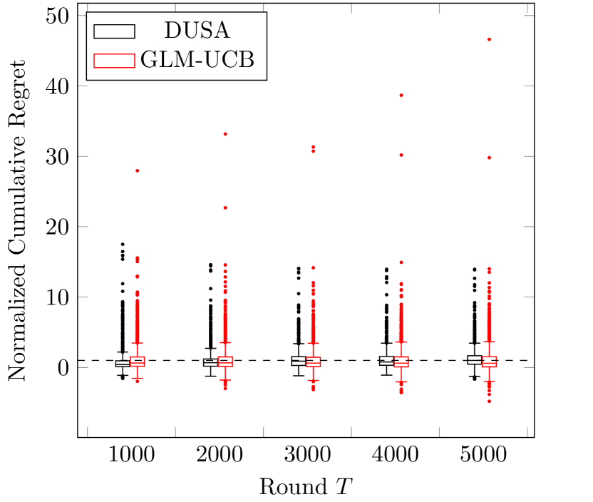
(a) Linear Bandit ($\abs{X}=5$)

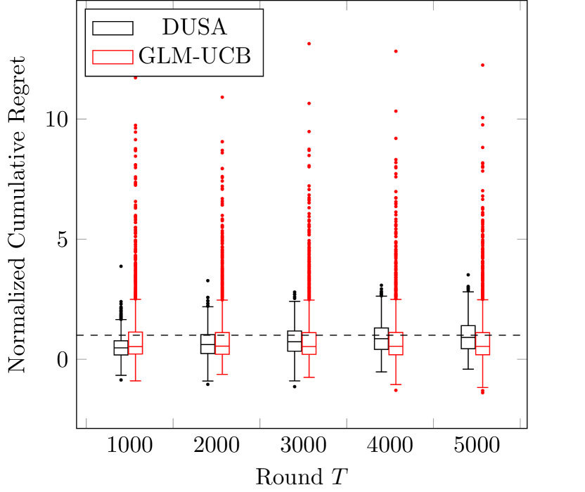
(b) Linear Bandit ($\abs{X}=15$)

Figure 5: The normalized cumulative regret of DUSA on linear bandit instances counting $\abs{X}=\{5,15\}$ arms as a function of the number of rounds $T$.

10 Topological Properties of the Information Distance

With a slight abuse of notation, we denote the set of all distributions supported on a set of outcomes $\setr$ as

$$\mathcal{P}_{\setr}=\tset{Q\in\real^{\abs{\setr}}_{+}}{\textstyle\sum_{r\in\setr}Q(r)=1}\,.$$ (53)

In this paper, we equip the probability simplex $\mathcal{P}_{\setr}$ with the standard topology relative to its affine hull. The open sets

$$\set{Q}{\textstyle\sum_{r\in\setr}Q(r)=1,~{}\norm{Q-P}_{\infty}\defn\norm{Q-P}_{\infty}=\max_{r\in\setr}\,\abs{Q(r)-P(r)}<\epsilon}$$

for all $P\in\mathcal{P}_{\setr}$ and $\epsilon>0$ are a base for this topology. The set of all interior points of $\mathcal{P}_{\setr}$ in this topology is then identified with $\tset{Q\in\real^{\abs{\setr}}_{++}}{\textstyle\sum_{r\in\setr}Q(r)=1}$. The information distance is a natural statistical notion of distance on the probability simplex $\mathcal{P}_{\setr}$ and satisfies several well-known key properties which we use in this paper.

Lemma 2 (Properties of Information Distance)

Let $\setr$ be a discrete set and $\mathcal{P}_{\setr}$ be the set defined in (53). The information distance enjoys the following key properties:

1. Information inequality. $I(P,P^{\prime})\geq 0$ for all $P,P^{\prime}\!\in\mathcal{P}_{\setr}$, and $I(P,P^{\prime})=0$ if and only if $P=P^{\prime}$.

2. Convexity. For all pairs $(P_{1},P^{\prime}_{1}),(P_{2},P^{\prime}_{2})\in\mathcal{P}_{\setr}\times\mathcal{P}_{\setr}$ and $\lambda\in[0,1]$ we have

   $$I\big{(}(1-\lambda)P_{1}+{\lambda}P_{2},(1-\lambda)P^{\prime}_{1}+\lambda P^{\prime}_{2}\big{)}\leq(1-\lambda)I(P_{1},P^{\prime}_{1})+\lambda I(P_{2},P^{\prime}_{2}).$$

3. Continuity in $P^{\prime}$. $I(P,P^{\prime})$ is continuous in $P^{\prime}$ on $\set{P^{\prime}\in{\mathcal{P}_{\setr}}}{P\ll P^{\prime}}$ for any fixed $P\in\mathcal{P}_{\setr}$.

4. Lower semi-continuity. $I$ is lower semicontinuous on $\mathcal{P}_{\setr}\times\mathcal{P}_{\setr}$. That is, its sub-level sets defined as $\set{(P,P^{\prime})\in\mathcal{P}_{\setr}\times\mathcal{P}_{\setr}}{I(P,P^{\prime})\leq\alpha}$ are closed (and bounded) for any $\alpha\geq 0$.

Proof.

Proof of Lemma 2. The information inequality and convexity properties can be found in most textbooks on information theory. For instance, see Theorem 2.6.3 and Theorem 2.7.2 in Cover and Thomas (2012), respectively. For showing the lower semi-continuity result, let us write $I(P,P^{\prime})$ as

$$I(P,P^{\prime})=\textstyle\sum_{r\in\setr}P(r)\log(\tfrac{P(r)}{P^{\prime}(r)})$$

for $P$ and $P^{\prime}$ in $\mathcal{P}_{\setr}$, where we use the convention $0\log(\tfrac{0}{a})=0$ and $b\log(\tfrac{b}{0})=\infty$ for all $a\geq 0$ and $b>0$. The lower semi-continuity property follows from the fact that functions of the type $(u,v)\mapsto u\log(\tfrac{u}{v})$ are lower semi-continuous and summation preserves lower semi-continuity; see (Bertsekas 2009, Proposition 1.1.5).

For continuity in $P^{\prime}$, let $\supp(P)=\set{r\in\setr}{P(r)>0}$ denote the support of distribution $P$. We can write

$$I(P,P^{\prime})=\textstyle\sum_{r\in\supp(P)}P(r)\log(\tfrac{P(r)}{P^{\prime}(r)}).$$

Continuity of $I(P,P^{\prime})$ in $P^{\prime}$ when $P\ll P^{\prime}$ follows from the immediate observation that the logarithm function $\log(\tfrac{P(r)}{P^{\prime}(r)})$ is indeed finite and continuous at any $P^{\prime}(r)>0$ for $r\in\supp(P)$. ∎

11 Duality Results

To show the duality results in this section, we make use of Section LABEL:app:duality, where supplementary materials for duality is presented.

11.1 Proof of Lemma 1

At a high level, we will show that the maximization problem (23) is the dual problem associated with the primal minimization problem (21) as discussed in Section LABEL:sec:constraint-qualification. However, the primal minimization problem (21) does not satisfy the constraint qualification conditions required by Proposition LABEL:prop:strong-duality-general and hence establishing strong duality directly is problematic. To overcome this challenge, we will show strong duality for a slightly perturbed distance function. By letting the perturbation vanish asymptotically, we will then obtain the stated strong duality result.

We introduce the following perturbed distance functions

$$\begin{array}[]{rl}\dis_{\gamma}(\eta,x^{\prime},P)=\min&\sum_{x\in\tilde{X}(P)}\eta(x)I(P(x),Q(x))+\gamma I(P(x^{\star}(P)),Q(x^{\star}(P)))\\ \st&Q\in\mathcal{K},\\ &\sum_{x\in X,\,r\in\setr}~{}Q(r,x)=\abs{X},\\ &\sum_{r\in\setr}rQ(r,x^{\prime})\geq\rew^{\star}(P)\end{array}$$ (58)

where the minimum is achieved, as by Lemma 2, its objective function is lower semi-continuous in $Q$ while its feasible domain is compact. The perturbed distance function can indeed be regarded as a penalty formulation of the conic minimization problem (21) with positive penalty term $I(P(x^{\star}(P)),Q(x^{\star}(P)))\geq 0$. That is, we have $I(P(x^{\star}(P)),Q(x^{\star}(P)))=0$ for any $P(x^{\star}(P))=Q(x^{\star}(P))$ and $I(P(x^{\star}(P)),Q(x^{\star}(P)))>0$ otherwise. It is hence evident by comparing problems (58) and (21) that

$$\begin{array}[]{rl@{\hspace{4em}}}\dis_{\gamma}(\eta,x^{\prime},P)\leq\dis(\eta,x^{\prime},P)=\min_{Q}&\sum_{x\in\tilde{X}(P)}\eta(x)I(P(x),Q(x))\hfil\hskip 40.00006pt\\ \st&Q\in\mathcal{K},\hfil\hskip 40.00006pt\\ &\sum_{x\in X,\,r\in\setr}Q(r,x)=\abs{X},\hfil\hskip 40.00006pt\\ &\sum_{r\in\setr}rQ(r,x^{\prime})\geq\rew^{\star}(P),\hfil\hskip 40.00006pt\\ &Q(x^{\star}(P))=P(x^{\star}(P))\hfil\hskip 40.00006pt\end{array}$$

for any $\gamma\geq 0$ and deceitful arm $x^{\prime}\in\xd(P)$. From Nesterov (2004, Theorem 1.3.1) it also follows that $\dis(\eta,x^{\prime},P)=\lim_{\gamma\to\infty}\dis_{\gamma}(\eta,x^{\prime},P)$ as the sublevel sets of the objective function in the perturbed minimization problem (58) are bounded for any $\gamma>0$.

We will identify a Lagrangian dual formulation for the perturbed minimization problem (58) with the help of the following perturbed dual function

$$\dual_{\gamma}(\eta,x^{\prime},P~{};~{}\mu):= \sum_{x\in\tilde{X}(P),r\in\setr}\chi_{-\infty}(\eta(x)\geq\lambda(r,x)+\beta+\alpha\cdot r\mb 1(x=x^{\prime}))+\alpha\rew^{\star}(P)+\abs{X}\beta+$$

$$\sum_{x\in\tilde{X}(P),r\in\setr}\eta(x)\log\left(\frac{\eta(x)-\lambda(r,x)-\beta-\alpha\cdot r\mb 1(x=x^{\prime})}{\eta(x)}\right)P(r,x)+$$

$$\sum_{x\in x^{\star}(P),r\in\setr}\gamma\log\left(\frac{\gamma-\lambda(r,x)-\beta}{\gamma}\right)P(r,x)+\sum_{x\in x^{\star}(P),r\in\setr}\chi_{-\infty}(\gamma\geq\lambda(r,x)+\beta).$$

Indeed, using this perturbed dual function we will show the following strong duality result.

Lemma 3 (Dual Formulation of the Perturbed Distance Function)

For any reward distribution $\optp\in\mathcal{P}$ and suboptimal deceitful arm $x^{\prime}\in\xd(\optp)$, the following strong duality equality holds.

$$\begin{array}[]{rl}\dis_{\gamma}(\eta,x^{\prime},\optp)=\sup_{\mu}&\dual_{\gamma}(\eta,x^{\prime},\optp~{};~{}\mu)\\ \st&\mu\in\real_{+}\times\real\times\mathcal{K}^{\star}.\end{array}$$ (61)

We indicate first that the strong duality result stated in Lemma 3 between the perturbed distance function and perturbed dual function implies the claimed result as an asymptotic case by letting $\gamma\to\infty$. Indeed, as the functions $\dis_{\gamma}$ and $\dual_{\gamma}$ are both non-decreasing in $\gamma$, and our strong duality result, we can write

$$\dis(\eta,x^{\prime},P) =\lim_{\gamma\to\infty}\dis_{\gamma}(\eta,x^{\prime},P)=\sup_{\gamma\geq 0}\dis_{\gamma}(\eta,x^{\prime},P)$$

$$=\sup_{\gamma\geq 0}\sup_{\mu\in\real_{+}\times\real\times\mathcal{K}^{\star}}\dual_{\gamma}(\eta,x^{\prime},P~{};~{}\mu)$$

$$=\sup_{\mu\in\real_{+}\times\real\times\mathcal{K}^{\star},\gamma\geq 0}\dual_{\gamma}(\eta,x^{\prime},P~{};~{}\mu)$$

$$=\sup_{\mu\in\real_{+}\times\real\times\mathcal{K}^{\star}}\lim_{\gamma\to\infty}\dual_{\gamma}(\eta,x^{\prime},P~{};~{}\mu)$$

where the final limit is identified with

$$\dual(\eta,x^{\prime},P~{};~{}\mu)= \lim_{\gamma\to\infty}\dual_{\gamma}(\eta,x^{\prime},P~{};~{}\mu)$$

$$= \textstyle\sum_{x\in\tilde{X}(P),r\in\setr}\eta(x)\log\left(\frac{\left(\eta(x)-\lambda(x,r)-\beta-\alpha\cdot r\mb 1(x=x^{\prime})\right)}{\eta(x)}\right)P(r,x)$$

$$\quad-\textstyle\sum_{x\in x^{\star}(P),~{}r\in\setr}\lambda(r,x)P(r,x)+\alpha\rew^{\star}(P)+\beta|\tilde{X}(P)|$$

$$\quad+\textstyle\sum_{x\in\tilde{X}(P),r\in\setr}\chi_{-\infty}(\eta(x)\geq\lambda(r,x)+\beta+\alpha\cdot r\mb 1(x=x^{\prime}))$$

from which the claimed result follows.

11.2 Proof of Lemma 3

We will prove Lemma 3 as a special case of the strong duality result stated in Proposition LABEL:prop:strong-duality-general stated in Section LABEL:sec:constraint-qualification. We first derive the associated dual function for the perturbed problem (58). Afterwards, we verify that the perturbed problem (58) satisfies the required constraint qualification conditions necessary to invoke Proposition LABEL:prop:strong-duality-general.

Perturbed dual function. The Lagrangian function associated with the perturbed minimization problem (58) which we introduce in Section LABEL:sec:constraint-qualification is

$$L_{\gamma}(\eta,x^{\prime},P,Q~{};~{}\mu)= \sum_{x\in\tilde{X}(P),r\in\setr}\left[\eta(x)P(r,x)\log\left(\frac{P(r,x)}{Q(r,x)}\right)-\eta(x)P(r,x)+\eta(x)Q(r,x)\right]$$

$$\qquad+\sum_{x\in x^{\star}(P),r\in\setr}\left[\gamma P(r,x)\log\left(\frac{P(r,x)}{Q(r,x)}\right)-\gamma P(r,x)+\gamma Q(r,x)\right]$$

$$\qquad-\sum_{x\in X,r\in\setr}Q(r,x)\lambda(r,x)+\beta\Big{(}\abs{X}-\sum_{x\in X,r\in\setr}Q(r,x)\Big{)}$$

$$\qquad+\alpha\Big{(}\rew^{\star}(P)-\sum_{r\in\setr}rQ(r,x^{\prime})\Big{)}$$

where $\mu=(\alpha,\beta,\lambda)\in\real_{+}\times\real\times\mathcal{K}^{\star}$. The Lagrangian function can be simplified significantly by grouping terms to

$$L_{\gamma}(\eta,x^{\prime},P,Q~{};~{}\mu)=$$

$$\qquad\sum_{x\in\tilde{X}(P),r\in\setr}\left[Q(r,x)\big{(}\eta(x)-\lambda(r,x)-\beta-\alpha\cdot r\mb 1(x=x^{\prime})\big{)}+\eta(x)P(r,x)\log\left(\frac{P(r,x)}{Q(r,x)}\right)\right]$$

$$\qquad+\sum_{x\in x^{\star}(P),r\in\setr}\left[Q(r,x)\big{(}\gamma-\lambda(r,x)-\beta\big{)}+\gamma P(r,x)\log\left(\frac{P(r,x)}{Q(r,x)}\right)\right]$$

$$\qquad+\alpha\rew^{\star}(P)+\abs{X}\beta-\sum_{x\in\tilde{X}(P)}\eta(x)-\abs{x^{\star}(P)}\gamma\,$$

where we used the fact that we only are interested in deceitful arms which by definition can not be optimal, i.e., $x^{\prime}\in\xd(P)\implies x^{\prime}\not\in x^{\star}(P)$. The dual function associated with the perturbed problem (58) is $\dual_{\gamma}(\eta,x^{\prime},P~{};~{}\mu)\defn\min_{Q\geq 0}\,L_{\gamma}(\eta,x^{\prime},P,Q~{};~{}\mu)$ and satisfies the weak duality inequality $\dual_{\gamma}(\eta,x^{\prime},P~{};~{}\mu)\leq\dis_{\gamma}(\eta,x^{\prime},P)$. The dual function can be expressed equivalently as

$$\dual_{\gamma}(\eta,x^{\prime},P~{};~{}\mu)$$

$$= \sum_{x\in\tilde{X}(P),r\in\setr}\inf_{q\geq 0}\left[q\big{(}\eta(x)-\lambda(r,x)-\beta-\alpha\cdot r\mb 1(x=x^{\prime})\big{)}+\eta(x)P(r,x)\log\left(\frac{P(r,x)}{q}\right)\right]$$

$$\qquad+\sum_{x\in x^{\star}(P),r\in\setr}\inf_{q\geq 0}\left[q\big{(}\gamma-\lambda(r,x)-\beta\big{)}+\gamma P(r,x)\log\left(\frac{P(r,x)}{q}\right)\right]$$

$$\qquad+\alpha\rew^{\star}(P)+\abs{X}\beta-\sum_{x\in\tilde{X}(P)}\eta(x)-\abs{x^{\star}(P)}\gamma$$

$$= \sum_{\{x\in\tilde{X}(P),r:\eta(x)P(r,x)=0\}}\chi_{-\infty}(\eta(x)\geq\lambda(r,x)+\beta+\alpha\cdot r\mb 1(x=x^{\prime}))$$

$$\qquad+\sum_{\{x\in\tilde{x}^{\star}(P),r:\gamma P(r,x)=0\}}\chi_{-\infty}(\gamma\geq\lambda(r,x)+\beta+\alpha\cdot r\mb 1(x=x^{\prime}))$$

$$\qquad+\sum_{\{x\in\tilde{X}(P),r:\eta(x)P(r,x)>0\}}P(r,x)\inf_{\theta\geq 0}\Big{[}\theta(\eta(x)-\lambda(r,x)-\beta-\alpha\cdot r\mb 1(x=x^{\prime}))-\eta(x)\log(\theta)\Big{]}$$

$$\qquad+\sum_{\{x\in x^{\star}(P),r:\gamma P(r,x)>0\}}P(r,x)\inf_{\theta\geq 0}\Big{[}\theta(\gamma-\lambda(r,x)-\beta)-\gamma\log(\theta)\Big{]}$$

$$\qquad+\alpha\rew^{\star}(P)+\abs{X}\beta-\sum_{x\in\tilde{X}(P)}\eta(x)-\abs{x^{\star}(P)}\gamma\,,$$

where we obtain the last equality by a change of variables $q$ to $P(r,x)\theta$. Recall that $\chi_{-\infty}(A)$ takes on the value $0$ when event $A$ happens and $-\infty$ otherwise. Finally, using the convex conjugacy relationship $\max_{\theta\geq 0}u\theta+\log(\theta)=-(1+\log(-u))+\chi_{+\infty}(u\leq 0)$, we can simplify the perturbed dual function to

$$\dual_{\gamma}(\eta,x^{\prime},P~{};~{}\mu)$$

$$= \sum_{x\in\tilde{X}(P),r\in\setr}\chi_{-\infty}(\eta(x)\geq\lambda(r,x)+\beta+\alpha\cdot r\mb 1(x=x^{\prime}))$$

$$\qquad+\sum_{x\in x^{\star}(P),r\in\setr}\chi_{-\infty}(\gamma\geq\lambda(r,x)+\beta+\alpha\cdot r\mb 1(x=x^{\prime}))$$

$$\qquad+\sum_{\{x\in\tilde{X}(P),r:\eta(x)P(r,x)>0\}}P(r,x)\eta(x)\left[1+\log\left(\frac{\eta(x)-\lambda(r,x)-\beta-\alpha\cdot r\mb 1(x=x^{\prime})}{\eta(x)}\right)\right]$$

$$\qquad+\sum_{\{x\in x^{\star}(P),r:\gamma P(r,x)>0\}}P(r,x)\gamma\left[1+\log\left(\frac{\gamma-\lambda(r,x)-\beta}{\gamma}\right)\right]$$

$$\qquad+\alpha\rew^{\star}(P)+\abs{X}\beta-\sum_{x\in\tilde{X}(P)}\eta(x)-\abs{x^{\star}(P)}\gamma$$

$$= \sum_{x\in\tilde{X}(P),r\in\setr}\chi_{-\infty}(\eta(x)\geq\lambda(r,x)+\beta+\alpha\cdot r\mb 1(x=x^{\prime}))$$

$$\qquad+\sum_{x\in x^{\star}(P),r\in\setr}\chi_{-\infty}(\gamma\geq\lambda(r,x)+\beta+\alpha\cdot r\mb 1(x=x^{\prime}))$$

$$\qquad+\sum_{x\in\tilde{X}(P),r\in\setr}\eta(x)\log\left(\frac{\eta(x)-\lambda(r,x)-\beta-\alpha\cdot r\mb 1(x=x^{\prime})}{\eta(x)}\right)P(r,x)$$

$$\qquad+\sum_{x\in x^{\star}(P),r\in\setr}\gamma\log\left(\frac{\gamma-\lambda(r,x)-\beta}{\gamma}\right)P(r,x)$$

$$\qquad+\alpha\rew^{\star}(P)+\abs{X}\beta.$$

Strong duality perturbed problem. We can obtain the strong duality result claimed in Lemma 3, i.e., the equality

$$\sup_{\mu\in\real_{+}\times\real\times\mathcal{K}^{\star}}\dual_{\gamma}(\eta,P,x^{\prime}~{};~{}\mu)=\dis_{\gamma}(\eta,x^{\prime},P)$$

by verifying that the Slater’s constraint qualification conditions required by Proposition LABEL:prop:strong-duality-general are satisfied. In the following, we find a Slater point for problem (58). Precisely, we identify a distribution $\bar{Q}$ in the interior of $\mathcal{P}$ which is strictly feasible, i.e., $\sum_{r\in\setr}r\bar{Q}(r,x^{\prime})>\rew^{\star}(P)$. To do so, we consider any distribution $U$ in the interior of $\mathcal{P}$; that is, $U\in\interior(\mathcal{P})$. Finding such an interior point is possible as we take that $\interior(\mathcal{P})\neq\emptyset$ as a standing assumption.

Let the distribution $Q_{\max}$ be a distribution which satisfies $\sum_{r\in\setr}rQ_{\max}(r,x^{\prime})=\rew_{\max}(x^{\prime},P)>\rew^{\star}(P)$ were the previous strict inequality is guaranteed by the fact that $x^{\prime}$ is a deceitful arm. Define $Q_{\theta}\defn Q_{\max}\cdot\theta+U\cdot(1-\theta)\in\mathcal{P}$ for all $\theta\in[0,1]$. We will show that for some values of $\theta$, the reward distribution ${Q_{\theta}}$ can serve as a Slater point. Let

$$\theta^{\prime}=\frac{\rew^{\star}(P)-\sum_{r\in\setr}rU(r,x^{\prime})}{\rew_{\max}(x^{\prime},P)-\sum_{r\in\setr}rU(r,x^{\prime})}\in[-\infty,1).$$

Observe that for any $\theta\in(\theta^{\prime},1]\bigcap[0,1)$ , we have that the distribution $Q_{\theta}\in\interior(\mathcal{P})$ satisfies $\sum_{r\in\setr}rQ_{\theta}(x^{\prime},r)>\rew^{\star}(P)$. Hence, the particular distribution $\bar{Q}=Q_{\bar{\theta}}$ with $\bar{\theta}=\tfrac{(\max\{\theta^{\prime},0\}+1)}{2}$ serves as a Slater point for problem (58). Note that as $\bar{Q}\in\interior(\mathcal{P})$ is also in the interior of $\mathcal{P}_{\Omega}$ and hence in the interior of the domain of the objective function of problem (58).

11.3 More on the Sufficient Information Condition

The dual-test function provides a convenient procedure to verify if enough information has been collected already to distinguish the empirical $P_{t}$ from its deceitful models; that is, whether or not $\dis(\tfrac{N_{t}}{\log(t)},x^{\prime},P_{t})\geq\overline{\dual}\left(\tfrac{N_{t}}{\log(t)},x^{\prime},P_{t}~{};~{}\mu_{t}\right)\geq 1+\epsilon$ for any deceitful arm $x^{\prime}\in\xd(P_{t})$. The strong duality results in Lemma 1, relates the information distance between $P_{t}$ and $\dis(x^{\prime},P_{t})$ and the dual function as

$$\dis(\tfrac{N_{t}}{\log(t)},x^{\prime},P_{t})=\max_{\mu(x^{\prime})}\set{\dual(\tfrac{N_{t}}{\log(t)},x^{\prime},P_{t}~{};~{}\mu(x^{\prime}))}{\mu(x^{\prime})\in\real_{+}\times\real\times\mc K^{\star}}.$$

Our sufficient information test however involves instead a seemingly unrelated restricted dual problem

$$\overline{\dual}\left(\tfrac{N_{t}}{\log(t)},x^{\prime},P_{t}~{};~{}\mu_{t}\right)$$

$$= \max_{\rho\geq 0,\,\mu(x^{\prime})}\set{\dual(\tfrac{N_{t}}{\log(t)},x^{\prime},P_{t}~{};~{}\mu(x^{\prime}))}{\rho\geq 0,\,\mu(x^{\prime})=\rho\cdot\mu_{t}(x^{\prime})\in\real_{+}\times\real\times\mc K^{\star}}$$

$$= ~{}~{}\max_{\rho\geq 0}~{}\,\set{\dual(\tfrac{N_{t}}{\log(t)},x^{\prime},P_{t}~{};~{}\rho\cdot\mu_{t}(x^{\prime}))}{\rho\geq 0}.$$

Nevertheless, we will argue here that also this restricted dual problem admits a satisfying interpretation as the information distance condition between $P_{t}$ and a certain set of deceitful distributions. Indeed, for any feasible dual variable $\mu=(\alpha,\beta,\lambda)$, arbitrary empirical reward distribution $P_{t}\in\mc P$, and deceitful arm $x^{\prime}\in\xd(P_{t})$, we define $\mc H(x^{\prime},P_{t}~{};~{}\mu)$ as the following set of reward distributions:

$$\set{Q}{\begin{array}[]{l}Q(x^{\star}(P_{t}))=P_{t}(x^{\star}(P_{t})),\\[5.0pt] \sum_{x\in X,\,r\in\setr}Q(r,x)\left(\lambda(r,x)+\beta+\alpha r\mb 1(x=x^{\prime})\right)\geq\beta\abs{X}+\alpha\rew^{\star}(P_{t})\end{array}}\,.$$ (64)

We point out that the previously defined set contains all deceitful distributions whenever the dual variable $\mu$ is dual feasible; that is, $\mc H(x^{\prime},P_{t}~{};~{}\mu)\supseteq\prob(x^{\prime},P_{t})$, where the set of deceitful distributions $\prob(x^{\prime},P_{t})$ is presented as the feasible set of the convex minimization problem (21). Obviously, any deceitful distribution will satisfy $Q(x^{\star}(P_{t}))=P_{t}(x^{\star}(P_{t}))$ by construction. That is, the reward distributions of the empirically optimal arms of $P_{t}$ are in full agreement with those of $Q$. We now show that any deceitful distribution will also satisfy the second constraint $\sum_{x\in X,\,r\in\setr}Q(r,x)\left(\lambda(r,x)+\beta+\alpha r\mb 1(x=x^{\prime})\right)\geq\beta\abs{X}+\alpha\rew^{\star}(P_{t})$ characterizing the set $\mc H(x^{\prime},P_{t}~{};~{}\mu)$. The first term $\sum_{x\in X,\,r\in\setr}Q(r,x)\lambda(r,x)$ is nonnegative because $Q\in\mc K$ and dual feasible variable $\lambda\in\mc K^{\star}$. The second term satisfies $\sum_{x\in X,\,r\in\setr}\beta Q(r,x)=\beta\abs{X}$ irrespective of the value of the dual variable $\beta$; see the second constraints in the minimization problem (21). For any dual feasible variable $\alpha\geq 0$, the final term satisfies the inequality $\sum_{x\in X,\,r\in\setr}Q(r,x)r\mb 1(x=x^{\prime})\geq\rew^{\star}(P_{t})$; see the third constraints of minimization Problem (21). Thus, we have indeed the claimed inclusion $\mc H(x^{\prime},P_{t}~{};~{}\mu)\supseteq\prob(x^{\prime},P_{t})$. The following lemma provides an interpretation of the sufficient information condition.

Lemma 4 (Dual-test Function)

Let $P\in\interior(\mc P)$ and $\eta>0$ and consider any deceitful arm $x^{\prime}\in\xd(P)$. For any dual feasible variable $\mu=(\alpha,\beta,\lambda)\in\real_{+}\times\real\times\mc K^{\star}$, the dual-test function is equal to

$$\begin{array}[]{rl}\overline{\dual}(\eta,x^{\prime},P~{};~{}\mu)=\min_{Q}&\textstyle\sum_{x\in\tilde{X}(P)}\eta(x)I(P(x),Q(x))\\[5.0pt] \st&Q\in\mc H(x^{\prime},P~{};~{}\mu).\end{array}$$ (67)

Proof.

See Appendix 11.4. ∎

The optimization problem (67), which states an alternative characterization of our dual-test function, bears some resemblance to the minimization problem (6), which characterizes the distance function $\dis$. While the objective function of two optimization problems is the same, in the minimization Problem (6), we enforce the distribution $Q$ to belong to the deceitful set $\prob(x^{\prime},P)$, whereas in the minimization problem (67), we enforce the same distribution belong to merely belong to the superset $\mc H(x^{\prime},P~{};~{}\mu)$. Thus, the condition $1\leq\overline{\dual}(\eta,x^{\prime},P~{};~{}\mu)$ implies that sufficient information has been obtained to distinguish the null hypothesis $P$ not only from its deceitful distributions $\prob(x^{\prime},P)$ but in fact from the entire superset $\mc H(x^{\prime},P~{};~{}\mu)$. The simple observation that distinguishing $P$ from the larger set $\mc H(x^{\prime},P~{};~{}\mu)$ must necessarily be harder from a statistical point of view than distinguishing $P$ merely from the smaller set of deceitful distributions $\prob(x^{\prime},P)$ explains the weak duality inequality $\overline{\dual}(\eta,x^{\prime},P~{};~{}\mu)\leq\dis(\eta,x^{\prime},P)$ for any feasible dual variable $\mu$. Strong duality can be interpreted as the existence of a feasible dual variable $\mu^{\star}$ so that the distance between $P$ and the sets $\mc H(x^{\prime},P;\mu^{\star})$ and $\prob(x^{\prime},P)$ is the same. That is, $\overline{\dual}(\eta,x^{\prime},P~{};~{}\mu^{\star})=\dis(\eta,x^{\prime},P)=\sum_{x\in\tilde{X}(P)}\eta(x)I(P(x),Q^{\star}(x))$ for some worst-case deceitful reward distribution $Q^{\star}\in\prob(x^{\prime},P)$. Under those circumstances, the hyperplane $\mc H(x^{\prime},P~{};~{}\mu^{\star})$ separates the deceitful reward distributions $\prob(x^{\prime},P)$ and the information ball $\tset{Q}{Q(x^{\star}(P))=P(x^{\star}(P)),\,\sum_{x\in\tilde{X}(P)}\eta(x)I(P(x),Q(x))\leq\dis(\eta,P,x^{\prime})}$ as implied by the necessary and sufficient KKT optimality conditions of minimization problem (6) and visually illustrated in Figure 6.

The previous discussion also offers additional insight into the deep and shallow update algorithms introduced before. The deep update Algorithm 3 minimizes the regret over all exploration rates $\eta$ and dual variables so that the reward distribution $P$ can be distinguished from its deceitful distributions $\prob(x^{\prime},P)$ with sufficient statistical power; that is, the deep update ensures that $\dis(\eta,x^{\prime},P)\geq 1$. The shallow update, on the other hand, merely minimizes the regret over the logarithmic rates $\eta$ so that the reward distribution $P$ can be distinguished from the superset $\mc H(x^{\prime},P~{};~{}\mu)$ associated with the dual variable $\mu$. That is, the shallow update ensures that $\overline{\dual}(\eta,x^{\prime},P~{};~{}\mu)\geq 1$.

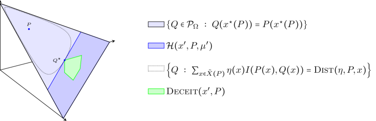
Figure 6: The sufficient information test $\overline{\dual}(\eta,x^{\prime},P~{};~{}\mu)\leq\dis(\eta,x^{\prime},P)$ for dual feasible variable $\mu$ quantifies the information distance between $P$ and the half-space $\mc H(x^{\prime},P~{};~{}\mu^{\prime})$ containing all deceitful distributions $\prob(x^{\prime},P)$. When $\mc H(x^{\prime},P~{};~{}\mu^{\star})$ for some $\mu^{\star}$ defines a separating half-space between $\prob(x^{\prime},P)$ and the information ball $\tset{Q}{Q(x^{\star}(P))=P(x^{\star}(P)),\,\sum_{x\in\tilde{X}(P)}\eta(x)I(P(x),Q(x))\leq\dis(\eta,P,x)}$, the information distance between $P$ and either the set of deceitful distributions $\prob(x^{\prime},P)$ or its superset $\mc H(x^{\prime},P~{};~{}\mu^{\prime})$ is the same. In that case, we have the strong duality equalities $\overline{\dual}(\eta,x^{\prime},P~{};~{}\mu^{*})=\dis(\eta,x^{\prime},P)=\sum_{x\in\tilde{X}(P)}\eta(x)I(P(x),Q^{\star}(x))$, where $Q^{\star}$ is the worst-case distribution, solving problem (67).

11.4 Proof of Lemma 4

The information minimization problem (67) can be written explicitly as

$$\begin{array}[]{rl@{~}l}\min&{\displaystyle\sum_{x\in\tilde{X}(P)}}\eta(x)I(P(x),Q(x))\hfil~{}&\\[10.00002pt] \st&{\displaystyle\sum_{x\in X,\,r\in\setr}}Q(r,x)\left[\lambda(r,x)\!+\!\beta\!+\!\alpha r\mb 1(x=x^{\prime})\right]\geq\beta\abs{X}+\alpha\rew^{\star}(P)\hfil~{}&[{\mathrm{dual~{}variable\!:\,}}\rho]\\[10.00002pt] &Q(x^{\star}(P))=P(x^{\star}(P))\hfil~{}&[{\mathrm{not~{}dualized}}]\end{array}$$ (71)

where we use the explicit characterization of $\mathcal{H}(x^{\prime},P~{};~{}\mu)$ given in Equation (64). We will claim first that the minimum in problem (71) is indeed attained. The remainder of the claimed results will be proven as a special strong duality result of the type discussed in Section LABEL:sec:constraint-qualification.

Attainment of minimum.

We first show that the minimum in (71) is in fact attained. The objective function of the information minimization problem has non-empty level sets

$$\set{Q\in\mathcal{H}(x^{\prime},P~{};~{}\mu)}{\textstyle\sum_{x\in\tilde{X}(P)}\eta(x)I(P(x),Q(x))\leq\gamma}$$

for any level $\gamma\geq\dis(\eta,x^{\prime},P)=\min_{Q\in\prob(x^{\prime},P)}\sum_{x\in\tilde{X}(P)}\eta(x)I(P(x),Q(x))$ as indeed we have the set inclusion $\prob(x^{\prime},P)\subseteq\mathcal{H}(x^{\prime},P~{};~{}\mu)$. These level sets are furthermore closed as the set $\mathcal{H}(x^{\prime},P~{};~{}\mu)$ is closed while the objective function is lower semi-continuous as per Lemma 2. Recall that we assume that the logarithmic rate $\eta>0$ is positive. Hence, the level sets are also bounded as we have

$$\set{Q\in\mathcal{H}(x^{\prime},P~{};~{}\mu)}{\textstyle\sum_{x\in\tilde{X}(P)}\eta(x)I(P(x),Q(x))\leq\gamma}$$

$$\subseteq\set{Q}{\eta(x)I(P(x),Q(x))\leq\gamma~{}~{}\forall x\in\tilde{X}(P),~{}Q(x^{\star}(P))=P(x^{\star}(P))}.$$

Bertsekas (2009, Prop. 3.2.1) guarantees that the set of minima in (71) is non-empty and compact.

Dual function.

The associated Lagrangian to the information minimization problem (71) introduced in Section LABEL:sec:constraint-qualification is equal to

$$\begin{array}[]{r@{~}l}L(\eta,x^{\prime},P,Q~{};~{}\rho)\defn~{}&\sum_{x\in\tilde{X}(P)}\eta(x)I(P(x),Q(x))\\ ~{}&~{}~{}+\rho(\sum_{x\in X,\,r\in\setr}Q(r,x)\left[-\lambda(r,x)-\beta-\alpha r\mb 1(x=x^{\prime})\right]+\beta\abs{X}+\alpha\rew^{\star}(P))\end{array}$$

which can be simplified further by collecting terms to

$$\begin{array}[]{r@{~}l}L(\eta,x^{\prime},P,Q~{};~{}\rho)=~{}&\sum_{x\in\tilde{X}(P),r\in\setr}Q(r,x)(-\rho\lambda(r,x)-\rho\beta-\rho\alpha r\mb 1(x=x^{\prime}))\\ ~{}&\quad+\sum_{x\in\tilde{X}(P)}\eta(x)I(P(x),Q(x))\\ ~{}&\quad+\sum_{x\in x^{\star}(P),r\in\setr}Q(r,x)(-\rho\lambda(r,x)-\rho\beta)+\rho\beta\abs{X}+\rho\alpha\rew^{\star}(P).\end{array}$$

The dual function associated with the perturbed problem (58) is as discussed in Section LABEL:sec:constraint-qualification identified with $g(\eta,x^{\prime},P~{};~{}\rho)\defn\min_{Q(x^{\star}(P))=P(x^{\star}(P))}\,L(\eta,x^{\prime},P,Q~{};~{}\rho).$ The dual function can be expressed equivalently as

$$g(\eta,x^{\prime},P~{};~{}\mu)$$

$$= \min_{Q(x^{\star}(P))=P(x^{\star}(P))}\sum_{x\in\tilde{X}(P),r\in\setr}Q(r,x)(-\rho\lambda(r,x)-\rho\beta-\rho\alpha r\mb 1(x=x^{\prime}))$$

$$\quad+\sum_{x\in\tilde{X}(P),r\in\setr}\eta(x)[P(r,x)\log\left(\textstyle\frac{P(r,x)}{Q(r,x)}\right)-P(r,x)+Q(r,x)]$$

$$\quad+\sum_{x\in x^{\star}(P),r\in\setr}Q(r,x)(-\rho\lambda(r,x)-\rho\beta)+\rho\beta\abs{X}+\rho\alpha\rew^{\star}(P)$$

$$= \sum_{x\in\tilde{X}(P),r\in\setr}\inf_{q\geq 0}\left[q\big{(}\eta(x)-\rho\lambda(r,x)-\rho\beta-\rho\alpha\cdot r\mb 1(x=x^{\prime})\big{)}+\eta(x)P(r,x)\log\left(\frac{P(r,x)}{q}\right)\right]$$

$$\qquad-\sum_{x\in x^{\star}(P)}\rho\lambda(r,x)P(r,x)+\rho\alpha\rew^{\star}(P)+\abs{\tilde{X}(P)}\beta\rho-\sum_{x\in\tilde{X}(P)}\eta(x)$$

$$= \sum_{\{x\in\tilde{X}(P),r:\eta(x)P(r,x)=0\}}\chi_{-\infty}(\eta(x)\geq\rho\lambda(r,x)+\rho\beta+\rho\alpha\cdot r\mb 1(x=x^{\prime}))$$

$$\qquad+\sum_{\{x\in\tilde{X}(P),r:\eta(x)P(r,x)>0\}}P(r,x)\inf_{\theta\geq 0}\Big{[}\theta(\eta(x)-\rho\lambda(r,x)-\rho\beta-\rho\alpha\cdot r\mb 1(x=x^{\prime}))-\eta(x)\log(\theta)\Big{]}$$

$$\qquad-\sum_{x\in x^{\star}(P)}\rho\lambda(r,x)P(r,x)+\rho\alpha\rew^{\star}(P)+\abs{\tilde{X}(P)}\rho\beta-\sum_{x\in\tilde{X}(P)}\eta(x)$$

where we obtain the last equality by a change of variables $q$ to $P(r,x)\theta$. Recall that $\chi_{-\infty}(A)$ takes on the value $0$ when event $A$ happens and $-\infty$ otherwise. Finally, using the convex conjugacy relationship $\max_{\theta\geq 0}u\theta+\log(\theta)=-(1+\log(-u))+\chi_{+\infty}(u\leq 0)$, we can simplify the perturbed dual function to

$$g(\eta,x^{\prime},P~{};~{}\rho)$$

$$= \sum_{x\in\tilde{X}(P),r\in\setr}\chi_{-\infty}(\eta(x)\geq\rho\lambda(r,x)+\rho\beta+\rho\alpha\cdot r\mb 1(x=x^{\prime}))$$

$$\qquad+\sum_{\{x\in\tilde{X}(P),r:\eta(x)P(r,x)>0\}}P(r,x)\eta(x)\left[1+\log\left(\frac{\eta(x)-\rho\lambda(r,x)-\rho\beta-\rho\alpha\cdot r\mb 1(x=x^{\prime})}{\eta(x)}\right)\right]$$

$$\qquad-\sum_{x\in x^{\star}(P)}\rho\lambda(r,x)P(r,x)+\rho\alpha\rew^{\star}(P)+\rho\abs{\tilde{X}(P)}\beta-\sum_{x\in\tilde{X}(P)}\eta(x)$$

$$= \sum_{x\in\tilde{X}(P),r\in\setr}\chi_{-\infty}(\eta(x)\geq\rho\lambda(r,x)+\rho\beta+\rho\alpha\cdot r\mb 1(x=x^{\prime}))$$

$$\qquad+\sum_{x\in\tilde{X}(P),r\in\setr}\eta(x)\log\left(\frac{\eta(x)-\rho\lambda(r,x)-\rho\beta-\rho\alpha\cdot r\mb 1(x=x^{\prime})}{\eta(x)}\right)P(r,x)$$

$$\qquad-\sum_{x\in x^{\star}(P)}\rho\lambda(r,x)P(r,x)+\rho\alpha\rew^{\star}(P)+\abs{\tilde{X}(P)}\rho\beta.$$

$$= \dual(\eta,x^{\prime},P~{};~{}\rho\cdot\mu).$$

Strong duality.

We can now obtain the strong duality equality

$$(\ref{eq:hypothesis-test-duality-2})=\max_{\rho\geq 0}~{}\dual(\eta,x^{\prime},P~{};~{}\rho\cdot\mu)$$

via Proposition LABEL:prop:strong-duality-general. Recall that the set $\prob(x^{\prime},P)\subseteq\mathcal{H}(x^{\prime},P,\mu)$ and hence in order to apply Proposition LABEL:prop:strong-duality-general, it suffices to construct a distribution $\bar{Q}\in\interior(\mathcal{P}_{\Omega})$ which satisfies

$$\textstyle\sum_{r\in\setr}\bar{Q}(r,x^{\prime})>\rew^{\star}(P)\quad{\mathrm{and}}\quad\bar{Q}(x^{\star}(P))=P(x^{\star}(P)).$$

Let $Q_{\theta}=\theta Q^{\star}+(1-\theta)P\in\mathcal{P}$ with $Q^{\star}$ a minimizer in problem (21). We will show there for some values of $\theta$, the reward distribution ${Q_{\theta}}$ can serve as a Slater point. Let

$$\theta^{\prime}=\frac{\rew^{\star}(P)-\sum_{r\in\setr}rP(r,x^{\prime})}{\rew_{\max}(x^{\prime},P)-\sum_{r\in\setr}rP(r,x^{\prime})}\in[-\infty,1).$$

Observe that as $P\in\interior(\mathcal{P})$ for any $\theta\in(\theta^{\prime},1]\bigcap[0,1)$, we have that the distribution $Q_{\theta}\in\interior(\mathcal{P})\subseteq\interior(\mathcal{P}_{\Omega})$ satisfies $\sum_{r\in\setr}rQ_{\theta}(x^{\prime},r)>\rew^{\star}(P)$. Hence, the particular distribution $\bar{Q}=Q_{\bar{\theta}}$ with $\bar{\theta}=\tfrac{(\max\{\theta^{\prime},0\}+1)}{2}$ serves as a Slater point for problem (71).

11.5 Dual Cones for Examples

Example 5 (Dual Cones)

In what follows, we discuss the cones $\mathcal{K}$ and its dual $\mathcal{K}^{\star}$ in the context of some of the example bandits discussed in Section 3.1. Detailed derivation of dual cones are deferred to Section 11.5.1.

1. Generic and separable bandits. Recall that the feasible set $\mathcal{P}$ of separable bandits is $\mathcal{P}=\textstyle\prod_{x\in X}\mathcal{P}_{x}$, where $\mathcal{P}_{x}$, $x\in X$, is a closed feasible set for the reward distribution of arm $x$. The cone $\mathcal{K}$ associated with feasible set $\mathcal{P}$ can be written as

   $$\mathcal{K} =\set{Q\in\real^{\abs{\setr}\times\abs{X}}_{+}}{\begin{array}[]{lr}\sum_{r\in\setr}Q(r,x)=\theta&\forall x\in X,\\ Q(x)\in\cone(\mathcal{P}_{x})&\forall x\in X.\end{array}}\,,$$ (74)

   The dual cone of the separable bandit cone $\mathcal{K}$ in Equation (74) is given as

   $$\mathcal{K}^{\star}=\set{\lambda\in\real^{\abs{\setr}\times\abs{X}}}{\begin{array}[]{lr}\exists\gamma(x)\in\real&\forall x\in X,\\ \lambda(x)-\textbf{1}\cdot\gamma(x)\in\cone(\mathcal{P}_{x})^{\star}&\forall x\in X,\\ \sum_{x\in X}\gamma(x)=0&\end{array}}\,,$$

   where 1 is the all ones vector with a size of $|\setr|$. This implies that when $\cone(\mathcal{P}_{x})^{\star}$ is efficiently representable for each arm, then $\mathcal{K}^{\star}$ admits an efficient barrier function.

2. Lipschitz Bernoulli bandits. Recall that the feasible set of Lipschitz Bernoulli Bandits is given by $\mathcal{P}_{\mathrm{Lips}}=\set{P\in\mathcal{P}_{\Omega}}{\begin{array}[]{lr}P(1,x)-P(1,x^{\prime})\leq L\cdot d(x,x^{\prime})&\forall x,x^{\prime}\in X\end{array}}$. Then, one can observe that the cone $\mathcal{K}$ associated with $\mathcal{P}_{\mathrm{Lips}}$ is given by

   $$\mathcal{K} =\set{Q\in\real^{2\times\abs{X}}_{+}}{\begin{array}[]{lr}\exists\theta\in\real,&\\ Q(0,x)+Q(1,x)=\theta&\forall x\in X,\\ Q(1,x)-Q(1,x^{\prime})\leq\theta\cdot L\cdot d(x,x^{\prime})&\forall x,x^{\prime}\in X\end{array}}\,.$$ (82)

   Note that the last constraint enforces the Lipschitz property of the reward distributions. The dual cone of the Lipschitz bandits cone $\mathcal{K}$ in Equation (82) is given as

   $$\mathcal{K}^{\star} =\set{\lambda\in\real^{2\times\abs{X}}}{\begin{array}[]{lr}\exists\Lambda(x,x^{\prime})\in\real_{+},~{}\exists\gamma(x)\in\real&\forall x,x^{\prime}\in X,\\ \lambda(1,x)+\sum_{x^{\prime}\in X}(\Lambda(x,x^{\prime})-\Lambda(x^{\prime},x))\geq\gamma(x)&\forall x\in X,\\ \lambda(0,x)\geq\gamma(x)&\forall x\in X,\\ \sum_{x\in X}\gamma(x)=L\sum_{x,x^{\prime}\in X}d(x,x^{\prime})\Lambda(x,x^{\prime})\end{array}}.$$

   The cone $\mathcal{K}^{\star}$ is here a polyhedral set implying that $\mathcal{K}^{\star}$ admits an efficient barrier function.

3. Parametric (linear) bandits. Recall that the feasible set of linear bandits is given by $\mc P_{\rm{lin}}=\set{Q\in\mc P_{\Omega}}{\forall x\in X,~{}\exists\theta~{}\st~{}\textstyle\sum_{r\in\setr}rQ(r,x)=c_{x}^{T}\theta}.$ Then, one can observe that the cone $\mathcal{K}$ associated with $\mathcal{P}_{\mathrm{lin}}$ is given by

   $$\mathcal{K} =\set{Q\in\real^{\abs{\setr}\times\abs{X}}_{+}}{\begin{array}[]{lr}\exists\theta,\theta^{\prime}\in\real,&\\ \sum_{r\in\setr}rQ(r,x)=\theta^{\prime}&\forall x\in X,\\ \sum_{r\in\setr}rQ(r,x)=c_{x}^{T}\theta&\forall x\in X\end{array}}\,.$$ (86)

   The dual cone of the linear bandits cone $\mathcal{K}$ in Equation (86) is given as

   $$\mathcal{K}^{\star} =\set{\lambda\in\real^{\abs{\setr}\times\abs{X}}}{\begin{array}[]{lr}\exists\nu(x)\in\real,~{}\exists\gamma(x)\in\real&\forall x\in X,\\ \lambda(r,x)\geq\gamma(x)+r\nu(x)&\forall r\in\setr,x\in X,\\ \sum_{x\in X}\gamma(x)=0,~{}\sum_{x\in X}c_{x}\nu(x)=0\end{array}}.$$

   The cone $\mathcal{K}^{\star}$ is here a polyhedral set, implying that $\mathcal{K}^{\star}$ admits an efficient barrier function.

4. Dispersion bandits. Recall that the feasible set of our dispersion bandits is given by $\mc P_{\rm{dis}}=\set{Q\in\mc P_{\Omega}}{\tfrac{\sum_{r\in\setr}r^{2}Q(r,x)}{\sum_{r\in\setr}rQ(r,x)}\leq\gamma(x)~{}~{}\forall x\in X}.$ Then, one can observe that the cone $\mathcal{K}$ associated with $\mathcal{P}_{\mathrm{dis}}$ is given by

   $$\mathcal{K} =\set{Q\in\real^{\abs{\setr}\times\abs{X}}_{+}}{\begin{array}[]{lr}\exists\theta\in\real,&\\ \sum_{r\in\setr}rQ(r,x)=\theta&\forall x\in X,\\ \sum_{r\in\setr}r^{2}Q(r,x)\leq\gamma(x)\sum_{r\in\setr}rQ(r,x)&\forall x\in X\end{array}}\,.$$ (90)

   The dual cone of the linear bandits cone $\mathcal{K}$ in Equation (86) is given as

   $$\mathcal{K}^{\star} =\set{\lambda\in\real^{\abs{\setr}\times\abs{X}}}{\begin{array}[]{lr}\exists\nu(x)\in\real_{+},~{}\exists\mu(x)\in\real&\forall x\in X,\\ \lambda(r,x)\geq\mu(x)-(r^{2}-\gamma(x)r)\nu(x)&\forall r\in\setr,x\in X,\\ \sum_{x\in X}\mu(x)=0\end{array}}.$$

   The cone $\mathcal{K}^{\star}$ is here a polyhedral set, implying that $\mathcal{K}^{\star}$ admits an efficient barrier function.

11.5.1 Detailed Derivation of Dual Cones

Dual cone of generic and separable bandits. From the definition of dual cones, it follows that $\lambda\in\mathcal{K}^{\star}\iff 0\leq\min_{Q\in\mathcal{K}}\iprod{\lambda}{Q}$, where for separable bandits, the cone $\mathcal{K}$ is given in Equation (74). Here, we have that the previous primal minimization problem $\min_{Q\in\mathcal{K}}\iprod{\lambda}{Q}$ can be characterized as

$$\begin{array}[]{rl@{\hspace{2em}}l@{\hspace{3em}}r}\min_{Q,\theta}&\iprod{\lambda}{Q}\hfil\hskip 20.00003pt&\hfil\hskip 30.00005pt&\\ \st&\sum_{r\in\setr}Q(r,x)=\theta\hfil\hskip 20.00003pt&\forall x\in X,\hfil\hskip 30.00005pt&[\mathrm{dual~{}variable~{}}\gamma\in\real^{\abs{X}}]\\ &Q(x)\in\cone(\mathcal{P}_{x})\hfil\hskip 20.00003pt&\forall x\in X,\hfil\hskip 30.00005pt&[\mathrm{dual~{}variable~{}}\Lambda(x)\in\cone(\mathcal{P}_{x})^{\star}]\end{array}$$ (94)

where the constraint of the above optimization problem enforces $Q$ to belong to cone $\mathcal{K}$; see Equation (74). Please remark that this is not the only possible valid optimization characterization. Nevertheless, its primal characterization will be found to have a particularly simple dual. We remark that the special case of generic bandit problems is subsumed in the separable bandit problem and corresponds to the particular choice $\cone(\mathcal{P}_{x})$ the positive orthant. The associated Lagrangian function as introduced in Section LABEL:sec:constraint-qualification is

$$\textstyle L_{\lambda}(Q,\theta~{};~{}\gamma,\Lambda)=\iprod{\lambda}{Q}+\sum_{x\in X}\gamma(x)(\theta-\sum_{x\in X,\,r\in\setr}Q(r,x))-\sum_{x\in X}\iprod{\Lambda(x)}{Q(x)}\,,$$

which can be simplified by collecting terms to

$$L_{\lambda}(Q,\theta~{};~{}\gamma,\Lambda)=\textstyle\sum_{x\in X,r\in\setr}(\lambda(r,x)-\gamma(x)-\Lambda(r,x))\cdot Q(r,x)+\theta\sum_{x\in X}\gamma(x)\,.$$

The associated dual function as introduced in Section LABEL:sec:constraint-qualification is hence

$$g_{\lambda}(\gamma,\Lambda)\defn\min_{Q,\theta}L_{\lambda}(Q,\theta~{};~{}\gamma,\Lambda)=\sum_{x\in X,r\in\setr}\chi_{-\infty}(\lambda(r,x)-\gamma(x)-\Lambda(r,x)=0)+\chi_{-\infty}(\sum_{x\in X}\gamma(x)=0)\,.$$

The sets $\cone(\mathcal{P}_{x})$ have non-empty interior, as $\interior(\prod_{x\in X}\mathcal{P}_{x})=\prod_{x\in X}\interior(\mathcal{P}_{x})$ is non-empty. Thus, the primal optimization problem (94) satisfies Slater’s constraint qualification and hence strong duality holds, per Proposition LABEL:prop:strong-duality-general. Hence, we have the equivalence

$$0\leq\min_{Q\in\mathcal{K}}\iprod{\lambda}{Q}=\max_{\gamma,\,\Lambda}g_{\lambda}(\gamma,\Lambda)\iff\left\{\begin{array}[]{lr}\exists\gamma(x)\in\real&\forall x\in X,\\ \lambda(x)-\textbf{1}\cdot\gamma(x)\in\cone(P_{x})^{\star}&\forall x\in X,\\ \sum_{x\in X}\gamma(x)=0.&\end{array}\right\}\iff\lambda\in\mathcal{K}^{\star}\,,$$

where 1 is the all ones vector of size of $|\setr|$.

Dual cone of Lipschitz bandits. Using the definition of dual cone, we again have $\lambda\in\mathcal{K}^{\star}\iff 0\leq\min_{Q\in\mathcal{K}}\iprod{\lambda}{Q}$, where for Lipschitz bandits, the cone $\mathcal{K}$ is given in Equation (82). Here, we have that the previous primal minimization problem $\min_{Q\in\mathcal{K}}\iprod{\lambda}{Q}$ can be characterized as

$$\begin{array}[]{rl@{\hspace{1em}}l@{\hspace{1em}}r}\min_{Q,\theta}&\iprod{\lambda}{Q}\hfil\hskip 10.00002pt&\hfil\hskip 10.00002pt&\\ \st&Q(0,x)+Q(1,x)=\theta,\hfil\hskip 10.00002pt&\forall x\in X\hfil\hskip 10.00002pt&[\mathrm{dual~{}variable~{}}\gamma\in\real]\\ &Q(1,x)-Q(1,x^{\prime})\leq\theta\cdot L\cdot d(x,x^{\prime})\hfil\hskip 10.00002pt&\forall x,x^{\prime}\in X,\hfil\hskip 10.00002pt&[\mathrm{dual~{}variable~{}}\Lambda\in\real^{\abs{X}\times\abs{X}}_{+}]\\ &Q\geq 0,\hfil\hskip 10.00002pt&\hfil\hskip 10.00002pt&[\mathrm{not~{}dualized}]\\ &\theta\in\real\hfil\hskip 10.00002pt&\hfil\hskip 10.00002pt&[\mathrm{not~{}dualized}]\end{array}$$ (103)

where the constraint of the above optimization problem enforces $Q$ to belong to cone $\mathcal{K}$; see Equation (82). Please remark that this is not the only possible valid characterization. Nevertheless, its primal characterization will be found to have a particularly simple dual. The associated Lagrangian function as introduced in Section LABEL:sec:constraint-qualification is

$$\textstyle L_{\lambda}(Q,\theta~{};~{}\gamma,\Lambda) =\textstyle\iprod{\lambda}{Q}+\sum_{x\in X}\gamma(x)(\theta-Q(0,x)-Q(1,x))$$

$$\qquad\textstyle+\sum_{x,x^{\prime}\in X}\Lambda(x,x^{\prime})(Q(1,x)-Q(1,x^{\prime})-\theta\cdot L\cdot d(x,x^{\prime})),$$

which can be simplified by collecting terms to

$$L_{\lambda}(Q,\theta~{};~{}\gamma,\Lambda)$$

$$=\textstyle\sum_{x\in X}(\lambda(0,x)-\gamma(x))\cdot Q(0,x)+\textstyle\theta(\sum_{x\in X}\gamma(x)-\sum_{x,x^{\prime}\in X}L\cdot d(x,x^{\prime})\cdot\Lambda(x,x^{\prime}))$$

$$\qquad\textstyle+\sum_{x\in X}\Big{(}\lambda(1,x)-\gamma(x)+\sum_{x^{\prime}\in X}\Lambda(x,x^{\prime})-\sum_{x^{\prime}\in X}\Lambda(x^{\prime},x)\Big{)}\cdot Q(1,x)\,.$$

The associated dual function as introduced in Section LABEL:sec:constraint-qualification is hence

$$g_{\lambda}(\gamma,\Lambda) \defn\min_{Q\geq 0,\,\theta}L_{\lambda}(Q,\theta~{};~{}\gamma,\Lambda)$$

$$\textstyle=\sum_{x\in X}\chi_{-\infty}(\lambda(0,x)-\gamma(x)\geq 0)$$

$$\qquad+\sum_{x\in X}\chi_{-\infty}(\lambda(1,x)-\gamma(x)+\sum_{x^{\prime}\in X}(\Lambda(x,x^{\prime})-\Lambda(x^{\prime},x))\geq 0)$$

$$\textstyle\qquad+\chi_{-\infty}(\sum_{x\in X}\gamma(x)=\sum_{x,x^{\prime}\in X}L\cdot d(x,x^{\prime})\cdot\Lambda(x,x^{\prime}))\,.$$

As the feasible set in (103) is a non-empty bounded polyhedron, strong linear duality holds. Hence, we have the equivalence

$$0\leq\min_{Q\in\mathcal{K}}\iprod{\lambda}{Q}=\max_{\gamma,\,\Lambda} ~{}g_{\lambda}(\gamma,\Lambda)\iff$$

$$\left\{\begin{array}[]{l@{\,}r}\exists\Lambda(x,x^{\prime})\in\real_{+},~{}\gamma(x)\in\real&\forall x,x^{\prime}\in X,\\ \lambda(0,x)\geq\gamma(x)&\forall x\in X,\\ \lambda(1,x)+\sum_{x^{\prime}\in X}\Lambda(x,x^{\prime})-\sum_{x^{\prime}\in X}\Lambda(x^{\prime},x)\geq\gamma(x)&\forall x\in X,\\ \sum_{x\in X}\gamma(x)=\sum_{x,x^{\prime}\in X}L\cdot d(x,x^{\prime})\cdot\Lambda(x,x^{\prime})&\end{array}\right\}.$$

Dual cone of linear bandits. Using the definition of dual cone, we again have $\lambda\in\mathcal{K}^{\star}\iff 0\leq\min_{Q\in\mathcal{K}}\iprod{\lambda}{Q}$, where for linear bandits, the cone $\mathcal{K}$ is given in Equation (86). Here, we have that the previous primal minimization problem $\min_{Q\in\mathcal{K}}\iprod{\lambda}{Q}$ can be characterized as

$$\begin{array}[]{rl@{\hspace{1em}}l@{\hspace{1em}}r}\min_{Q,\theta,\theta^{\prime}}&\iprod{\lambda}{Q}\hfil\hskip 10.00002pt&\hfil\hskip 10.00002pt&\\ \st&\sum_{r\in\setr}Q(r,x)=\theta^{\prime}\hfil\hskip 10.00002pt&\forall x\in X,\hfil\hskip 10.00002pt&[\mathrm{dual~{}variable~{}}\gamma\in\real]\\ &\sum_{r\in\setr}rQ(r,x)=c_{x}^{T}\theta\hfil\hskip 10.00002pt&\forall x\in X,\hfil\hskip 10.00002pt&[\mathrm{dual~{}variable~{}}\nu\in\real^{\abs{X}}]\\ &Q\geq 0,\hfil\hskip 10.00002pt&\hfil\hskip 10.00002pt&[\mathrm{not~{}dualized}]\\ &\theta,\theta^{\prime}\in\real\hfil\hskip 10.00002pt&\hfil\hskip 10.00002pt&[\mathrm{not~{}dualized}]\end{array}$$ (109)

The associated Lagrangian function as introduced in Section LABEL:sec:constraint-qualification is

$$\textstyle L_{\lambda}(Q,\theta,\theta^{\prime}~{};~{}\gamma,\nu) =\textstyle\iprod{\lambda}{Q}\!+\!\sum_{x\in X}\gamma(x)(\theta^{\prime}\!-\!\sum_{r\in\setr}Q(r,x))\textstyle\!+\!\sum_{x\in X}\nu(x)(c_{x}^{T}\theta\!-\!\sum_{r\in\setr}rQ(r,x)),$$

which can be simplified by collecting terms to

$$L_{\lambda}(Q,\theta,\theta^{\prime}~{};~{}\gamma,\nu)=\textstyle\sum_{r\in\setr,x\in X}(\lambda(r,x)\!-\!\gamma(x)\!-\!r\nu(x))\cdot Q(r,x)\!+\!\theta^{\prime}\sum_{x\in X}\gamma(x)\!+\!\sum_{x\in X}\nu(x)c_{x}^{T}\theta.$$

The associated dual function as introduced in Section LABEL:sec:constraint-qualification is hence

$$g_{\lambda}(\gamma,\nu) \defn\min_{Q\geq 0,\,\theta,\theta^{\prime}}L_{\lambda}(Q,\theta,\theta^{\prime}~{};~{}\gamma,\nu)$$

$$\textstyle=\sum_{r\in\setr,x\in X}\chi_{-\infty}(\lambda(r,x)\!-\!\gamma(x)\!-\!r\nu(x)\geq 0)$$

$$\qquad\textstyle+\chi_{-\infty}(\sum_{x\in X}\gamma(x)=0)+\chi_{-\infty}(\sum_{x\in X}\nu(x)c_{x}=0).$$

As the feasible set in (109) is a non-empty bounded polyhedron, strong linear duality holds. Hence, we have the equivalence

$$0\leq\min_{Q\in\mathcal{K}}\iprod{\lambda}{Q}=\max_{\gamma,\,\nu} ~{}g_{\lambda}(\gamma,\nu)\iff$$

$$\left\{\begin{array}[]{lr}\exists\nu(x)\in\real,~{}\exists\gamma(x)\in\real&\forall x\in X,\\ \lambda(r,x)\geq\gamma(x)+r\nu(x)&\forall r\in\setr,x\in X,\\ \sum_{x\in X}\gamma(x)=0,~{}\sum_{x\in X}c_{x}\nu(x)=0\end{array}\right\}.$$

Dual cone of Dispersion bandits. Using the definition of dual cone, we again have $\lambda\in\mathcal{K}^{\star}\iff 0\leq\min_{Q\in\mathcal{K}}\iprod{\lambda}{Q}$, where for dispersion bandits, the cone $\mathcal{K}$ is given in Equation (90). Here, we have that the previous primal minimization problem $\min_{Q\in\mathcal{K}}\iprod{\lambda}{Q}$ can be characterized as

$$\begin{array}[]{rl@{\hspace{1em}}l@{\hspace{1em}}r}\min_{Q,\theta,\theta^{\prime}}&\iprod{\lambda}{Q}\hfil\hskip 10.00002pt&\hfil\hskip 10.00002pt&\\ \st&\sum_{r\in\setr}Q(r,x)=\theta^{\prime}\hfil\hskip 10.00002pt&\forall x\in X,\hfil\hskip 10.00002pt&[\mathrm{dual~{}variable~{}}\mu\in\real]\\ &\sum_{r\in\setr}r^{2}Q(r,x)\leq\gamma(x)\sum_{r\in\setr}rQ(r,x)\hfil\hskip 10.00002pt&\forall x\in X,\hfil\hskip 10.00002pt&[\mathrm{dual~{}variable~{}}\nu\in\real^{\abs{X}}_{+}]\\ &Q\geq 0,\hfil\hskip 10.00002pt&\hfil\hskip 10.00002pt&[\mathrm{not~{}dualized}]\\ &\theta\in\real\hfil\hskip 10.00002pt&\hfil\hskip 10.00002pt&[\mathrm{not~{}dualized}]\end{array}$$ (115)

The associated Lagrangian function as introduced in Section LABEL:sec:constraint-qualification is

$$\textstyle L_{\lambda}(Q,\theta~{};~{}\mu,\nu) =\textstyle\iprod{\lambda}{Q}\!+\!\sum_{x\in X}\mu(x)(\theta\!-\!\sum_{r\in\setr}Q(r,x))\textstyle\!+\!\sum_{r\in\setr,x\in X}\nu(x)(r^{2}Q(r,x)-\gamma(x)rQ(r,x)),$$

which can be simplified by collecting terms to

$$L_{\lambda}(Q,\theta~{};~{}\mu,\nu)=\textstyle\sum_{r\in\setr,x\in X}(\lambda(r,x)\!-\!\mu(x)\!+\!(r^{2}-r\gamma(x))\nu(x))\cdot Q(r,x)\!+\!\theta\sum_{x\in X}\mu(x).$$

The associated dual function as introduced in Section LABEL:sec:constraint-qualification is hence

$$g_{\lambda}(\mu,\nu) \defn\min_{Q\geq 0,\,\theta,\theta^{\prime}}L_{\lambda}(Q,\theta,~{};~{}\mu,\nu)$$

$$\textstyle=\sum_{r\in\setr,x\in X}\chi_{-\infty}(\lambda(r,x)\!-\!\mu(x)\!+\!(r^{2}-r\gamma(x))\nu(x)\geq 0)\textstyle+\chi_{-\infty}(\sum_{x\in X}\mu(x)=0).$$

As the feasible set in (115) is a non-empty bounded polyhedron, strong linear duality holds. Hence, we have the equivalence

$$0\leq\min_{Q\in\mathcal{K}}\iprod{\lambda}{Q}=\max_{\mu,\,\nu} ~{}g_{\lambda}(\mu,\nu)\iff$$

$$\left\{\begin{array}[]{lr}\exists\nu(x)\in\real_{+},~{}\exists\mu(x)\in\real&\forall x\in X,\\ \lambda(r,x)\geq\mu(x)-(r^{2}-\gamma(x)r)\nu(x)&\forall r\in\setr,x\in X,\\ \sum_{x\in X}\mu(x)=0\end{array}\right\}.$$

12 Proof of Theorem 3: Regret Bound of DUSA

We first present our concentrations bound and explain how the regret of DUSA can be decomposed.

12.1 Concentration Bounds and Regret Decomposition

We start with presenting our supporting concentration bounds. These bounds will be used multiple times throughout the proof and their proofs are presented in Appendix LABEL:sec:proof:concentration.

Lemma 5 (Concentration Bound)

For any arm $x\in X$, let

References

- Agrawal et al. (1989) Agrawal R, Teneketzis D, Anantharam V (1989) Asymptotically efficient adaptive allocation schemes for controlled iid processes: Finite parameter space. IEEE Transactions on Automatic Control 34(3).
- Aubin and Frankowska (2009) Aubin JP, Frankowska H (2009) Set-Valued Analysis (Springer Science & Business Media).
- Balseiro et al. (2019) Balseiro S, Golrezaei N, Mahdian M, Mirrokni V, Schneider J (2019) Contextual bandits with cross-learning. Advances in Neural Information Processing Systems, 9676–9685.
- Bank et al. (1982) Bank B, Guddat J, Klatte D, Kummer B, Tammer K (1982) Non-Linear Parametric Optimization (Springer).
- Barvinok (2002) Barvinok A (2002) A Course in Convexity, volume 54 (American Mathematical Society).
- Berge (1997) Berge C (1997) Topological Spaces: Including a Treatment of Multi-Valued Functions, Vector Spaces, and Convexity (Courier Corporation).
- Bertsekas (2009) Bertsekas D (2009) Convex Optimization Theory (Athena Scientific Belmont).
- Besbes and Zeevi (2009) Besbes O, Zeevi A (2009) Dynamic pricing without knowing the demand function: Risk bounds and near-optimal algorithms. Operations Research 57(6):1407–1420.
- Boyd and Vandenberghe (2004) Boyd S, Vandenberghe L (2004) Convex Optimization (Cambridge University Press).
- Bubeck and Cesa-Bianchi (2012) Bubeck S, Cesa-Bianchi N (2012) Regret analysis of stochastic and nonstochastic multi-armed bandit problems. Foundations and Trends® in Machine Learning 5(1):1–122.
- Bubeck et al. (2019) Bubeck S, Devanur N, Huang Z, Niazadeh R (2019) Multi-scale online learning: Theory and applications to online auctions and pricing. Journal of Machine Learning Research .
- Cappé et al. (2013) Cappé O, Garivier A, Maillard OA, Munos R, Stoltz G (2013) Kullback-leibler upper confidence bounds for optimal sequential allocation. The Annals of Statistics 41(3):1516–1541.
- Chandrasekaran and Shah (2017) Chandrasekaran V, Shah P (2017) Relative entropy optimization and its applications. Mathematical Programming 161(1-2):1–32.
- Combes et al. (2017) Combes R, Magureanu S, Proutiere A (2017) Minimal exploration in structured stochastic bandits. Advances in Neural Information Processing Systems, 1763–1771.
- Combes and Proutiere (2014) Combes R, Proutiere A (2014) Unimodal bandits: Regret lower bounds and optimal algorithms. International Conference on Machine Learning, 521–529.
- Combettes (2018) Combettes P (2018) Perspective functions: Properties, constructions, and examples. Set-Valued and Variational Analysis 26(2):247–264.
- Cover and Thomas (2012) Cover T, Thomas J (2012) Elements of Information Theory (John Wiley & Sons).
- Dani et al. (2008) Dani V, Hayes T, Kakade S (2008) Stochastic linear optimization under bandit feedback. International Conference on Algorithmic Learning Theory, 355–366.
- Filippi et al. (2010) Filippi S, Cappe O, Garivier A, Szepesvári C (2010) Parametric bandits: The generalized linear case. NIPS, volume 23, 586–594.
- Garivier and Cappé (2011) Garivier A, Cappé O (2011) The KL-UCB algorithm for bounded stochastic bandits and beyond. Proceedings of the 24th annual conference on learning theory, 359–376.
- Golrezaei et al. (2019) Golrezaei N, Javanmard A, Mirrokni V (2019) Dynamic incentive-aware learning: Robust pricing in contextual auctions. Advances in Neural Information Processing Systems, 9756–9766.
- Graves and Lai (1997) Graves T, Lai T (1997) Asymptotically efficient adaptive choice of control laws incontrolled Markov chains. SIAM Journal on Control and Optimization 35(3):715–743.
- Gupta et al. (2021) Gupta S, Chaudhari S, Joshi G, Yağan O (2021) Multi-armed bandits with correlated arms. IEEE Transactions on Information Theory 67(10):6711–6732.
- Gupta et al. (2020) Gupta S, Chaudhari S, Mukherjee S, Joshi G, Yağan O (2020) A unified approach to translate classical bandit algorithms to the structured bandit setting. IEEE Journal on Selected Areas in Information Theory 1(3):840–853.
- Hoeffding (1994) Hoeffding W (1994) Probability inequalities for sums of bounded random variables. The Collected Works of Wassily Hoeffding, 409–426 (Springer).
- Jun and Zhang (2020) Jun KS, Zhang C (2020) Crush optimism with pessimism: Structured bandits beyond asymptotic optimality. Advances in Neural Information Processing Systems 33.
- Kaufmann et al. (2012) Kaufmann E, Korda N, Munos R (2012) Thompson sampling: An asymptotically optimal finite-time analysis. International Conference on Algorithmic Learning Theory, 199–213 (Springer).
- Keskin and Zeevi (2014) Keskin N, Zeevi A (2014) Dynamic pricing with an unknown demand model: Asymptotically optimal semi-myopic policies. Operations Research 62(5):1142–1167.
- Lai and Robbins (1985) Lai T, Robbins H (1985) Asymptotically efficient adaptive allocation rules. Advances in applied mathematics 6(1):4–22.
- Lattimore and Munos (2014) Lattimore T, Munos R (2014) Bounded regret for finite-armed structured bandits. Advances in Neural Information Processing Systems 27:550–558.
- Lattimore and Szepesvari (2017) Lattimore T, Szepesvari C (2017) The end of optimism? an asymptotic analysis of finite-armed linear bandits. volume 54 of Proceedings of Machine Learning Research, 728–737 (Fort Lauderdale, FL, USA: PMLR).
- Magureanu et al. (2014) Magureanu S, Combes R, Proutiere A (2014) Lipschitz bandits: Regret lower bound and optimal algorithms. Conference on Learning Theory, volume 35 of Proceedings of Machine Learning Research, 975–999 (PMLR).
- Mao et al. (2018) Mao J, Leme R, Schneider J (2018) Contextual pricing for Lipschitz buyers. Advances in Neural Information Processing Systems, 5643–5651.
- Mersereau et al. (2009) Mersereau A, Rusmevichientong P, Tsitsiklis J (2009) A structured multiarmed bandit problem and the greedy policy. IEEE Transactions on Automatic Control 54(12):2787–2802.
- Nesterov (2004) Nesterov Y (2004) Introductory Lectures on Convex Optimization: A Basic Course (Kluwer Academic Publishers).
- Niazadeh et al. (2020) Niazadeh R, Golrezaei N, Wang J, Susan F, Badanidiyuru A (2020) Online learning via offline greedy: Applications in market design and optimization. Available at SSRN 3613756 .
- Rusmevichientong and Tsitsiklis (2010) Rusmevichientong P, Tsitsiklis JN (2010) Linearly parameterized bandits. Mathematics of Operations Research 35(2):395–411.
- Russo and Van Roy (2018) Russo D, Van Roy B (2018) Learning to optimize via information-directed sampling. Operations Research 66(1):230–252.
- Slivkins (2011) Slivkins A (2011) Contextual bandits with similarity information. Proceedings of the 24th annual Conference On Learning Theory, 679–702.
- Streeter and Golovin (2008) Streeter M, Golovin D (2008) An online algorithm for maximizing submodular functions. Advances in Neural Information Processing Systems, 1577–1584.
- Thompson (1933) Thompson W (1933) On the likelihood that one unknown probability exceeds another in view of the evidence of two samples. Biometrika 25(3/4):285–294.
- Zhang et al. (2020) Zhang M, Shen Z, Mokhtari A, Hassani H, Karbasi A (2020) One sample stochastic frank-wolfe. International Conference on Artificial Intelligence and Statistics, 4012–4023 (PMLR).