Gravitational Waves from Neutrino Emission Asymmetries in Core-Collapse Supernovae

Abstract

We present a broadband spectrum of gravitational waves from core-collapse supernovae (CCSNe) sourced by neutrino emission asymmetries for a series of full 3D simulations. The associated gravitational wave strain probes the long-term secular evolution of CCSNe and small-scale turbulent activity and provides insight into the geometry of the explosion. For non-exploding models, both the neutrino luminosity and the neutrino gravitational waveform will encode information about the spiral SASI. The neutrino memory will be detectable for a wide range of progenitor masses for a galactic event. Our results can be used to guide near-future decihertz and long-baseline gravitational-wave detection programs, including aLIGO, the Einstein Telescope, and DECIGO.

1 Introduction

Core-collapse supernova (CCSNe) explosions are dynamical events involving extreme astrophysical conditions, with the central core reaching super-nuclear densities and temperatures of hundreds of billions Kelvin. The relevant timescales in CCSNe range from sub-milliseconds to seconds, the former associated with the dynamical bounce, rotation, and convective motions and the latter due to secular evolution of the late-time neutrino emissions and explosion debris. No viable CCSNe explosion is spherical (Radice et al. 2017; Vartanyan et al. 2019b; Nagakura et al. 2019; Burrows et al. 2019; Burrows et al. 2020; Müller 2019b, with the possible exception of low-mass $\leq$9.5 M_⊙ progenitors which have very steep density profiles and weakly-bound mantles, see e.g. Radice et al. 2017). In general, multi-dimensional effects are critical to both modeling a successful explosion itself, and parametrized turbulence in spherically-symmetric 1D models (Mabanta et al. 2019; Couch et al. 2020) is less than adequate. Due to time-changing quadrupolar motions, CCSNe are classic sources of gravitational waves (GWs), with most of the gravitational-wave energy ($\sim$10^-8 M${}_{\odot}\mathrm{c}^{2}$, where M_⊙ indicates a solar mass) coming out at 100s to 1000s of Hertz. A major discriminating spectral signature is the g-mode/f-mode of fundamental oscillation of the proto-neutron star (PNS) that evolves to higher frequencies as the core deleptonizes and cools on its way to the cold, catalyzed neutron star state. This mode is excited by asymmetrically infalling plumes of matter that hammer the PNS in the first seconds of core-collapse and explosion and is an important asteroseismological measure of core structure and early evolution. The modern theory of this dominant GW component of core-collapse supernovae is summarized in Morozova et al. (2018) and in Radice et al. (2019), and in references therein (see also Sotani et al. 2017; Torres-Forné et al. 2018, 2019; Mezzacappa et al. 2020).

However, the low-frequency component below $\sim$10 Hz, not so easily measured even by next generation ground-based platforms, bears the stamp of important secular motions. The first is due to ejecta motions themselves. The explosions are generically asymmetrical, with matter ejection and core recoil kicks on 0.1 to a few seconds timescales (Burrows & Hayes, 1996; Murphy et al., 2009; Holgado & Ricker, 2019). Interestingly, the metric perturbations do not necessarily return to zero, and the metric is permanently shifted. This is akin to the classical “memory” effect (Christodoulou, 1991; Thorne, 1992), but is due to asymmetrical matter ejection. The associated frequencies are $\sim$0.1 to 10 Hz. It is thought that pulsars are born with kicks due either to asymmetrical ejecta or to asymmetrical neutrino emission and the associated momentum recoils. Though momentum asymmetries are dipolar phenomena, there is always an associated quadrupolar component (Vartanyan et al., 2019b).

Along with the longer-term secular matter component at low frequencies, intriguingly there is a similar contribution due to asymmetrical neutrino emissions (Epstein, 1978; Turner, 1978; Braginskii & Thorne, 1987; Burrows & Hayes, 1996; Müller & Janka, 1997; Kotake et al., 2006; Kotake et al., 2009b; Kotake, 2010; Kotake et al., 2011; Müller et al., 2012, 2013; Li et al., 2018). The neutrinos move at (very near) the speed of light, involve $\sim$0.1 to $\sim$0.3 solar masses equivalent, and are generically emitted aspherically (see, e.g., Tamborra et al. 2013; Vartanyan et al. 2019b; Walk et al. 2019). The shells of outgoing neutrinos constitute time-changing quadrupoles that source gravitational radiation at frequencies of $\sim$0.1 to 10 Hz (Burrows & Hayes, 1996; Müller & Janka, 1997; Müller et al., 2012). The high bulk mass-energy and speed of the neutrinos result in their almost complete domination over the matter component for low-frequency gravitational-waves in the GW spectrum of CCSNe. While the high-frequency component might boast a product of distance and metric strain ($h_{+}D$) of a few centimeters, the neutrino component at those low frequencies is $\sim$10-100 centimeters. However, due to the much lower frequencies and the squared frequency dependence, the energy in this component is much smaller ($\sim$a few $\times$ 10^-12 M${}_{\odot}c^{2}$) than found from the fundamental f-mode signal due to PNS oscillation (Radice et al., 2019). Nevertheless, the neutrino part of the CCSNe GW signature at frequencies of 0.1 to 10 Hz could be detected by a variety of proposed space- and ground-based GW interferometers (Arca Sedda et al., 2019; Yagi & Seto, 2011; Sato et al., 2017; Punturo et al., 2010; Maggiore et al., 2020; Aasi et al., 2015). Stamped on these GW data would be information on the asymmetry of matter and neutrino emissions and characteristic timescales of explosion and neutron star formation (Braginskii & Thorne, 1987; Burrows & Hayes, 1996; Müller et al., 2012; Vartanyan et al., 2019b). Hence, the low-frequency channels complement those at higher frequencies to provide a richer picture of supernova dynamics. This would complement the science gleaned from the direct neutrino emissions themselves. In fact, the GW data across the full GW spectral range provides added value $-$ joint GW/neutrino analysis would yield returns that are greater than the sum of the individual parts.

Simulation studies over the last decade have explored the contribution of matter motions, from convective structure to large-scale instabilities such as the SASI (Foglizzo, 2002; Blondin & Shaw, 2007; Foglizzo et al., 2012), to the development of gravitational waves in 2D and 3D simulations and their subsequent detection (Vartanyan et al., 2019b; Radice et al., 2019; Morozova et al., 2018; Andresen et al., 2017, 2019; Powell & Müller, 2019, 2020). Studies have also explored information to be gleaned from detections of neutrino signals with upcoming detectors, such as DUNE and HyperKamiokande (Wallace et al., 2016; Seadrow et al., 2018; Vartanyan et al., 2019b; Müller, 2019a; Kuroda et al., 2017). This progress has paralleled growth in detailed multi-dimensional simulations of CCSNe, many producing robust explosions (Vartanyan et al., 2018, 2019a; Radice et al., 2018; Burrows et al., 2019; Burrows et al., 2020; Nagakura et al., 2019; Summa et al., 2018; O’Connor & Couch, 2018; Müller et al., 2017; Yoshida et al., 2019; Roberts et al., 2016; Kuroda et al., 2020; Ott et al., 2018).

Less effort, however, has been dedicated to gravitational waveforms from neutrino memory (Burrows & Hayes, 1996; Kotake et al., 2007; Kotake et al., 2009b; Müller et al., 2012, 2013). Moreover, such studies have either been 2D simulations, or 3D with parameterized neutrino heating. The contribution to gravitational waves from neutrino anisotropies have not been recently studied despite the fact that gravitational waves from CCSNe provide promising candidates for third generation gravitational-wave detectors (Cavagliá et al., 2020; Arca Sedda et al., 2019; Srivastava et al., 2019; Schmitz, 2020).

Here, we explore gravitational wave signatures from neutrino anisotropies for 13 progenitors from 9$-$60 M_⊙, all evolved in 3D with our code Fornax (Skinner et al., 2019). These models were described in Burrows et al. (2019); Burrows et al. (2020). The paper is outlined as follows: in Sec 2, we summarize the numerical setup of our simulations and introduce the mathematical framework for studying gravitational waveforms from neutrino anisotropies. In Sec. 3, we describe our results and explore gravitational waves from neutrino anisotropies as probes of turbulent CCSNe dynamics. We discuss the frequency dependence of the GW signal and the resulting prospects for future detection. We present our conclusions in Sec 4.

2 Numerical Setup

Fornax (Skinner et al., 2019) is a multi-dimensional, multi-group radiation hydrodynamics code originally constructed to study core-collapse supernovae. It features an M1 solver for neutrino transport with detailed neutrino microphysics and a monopole approximation to general relativity (Marek & Janka 2009). In this paper, we study 13 stellar progenitors in 3D, with ZAMS (Zero Age Main Sequence) masses of 9, 10, 12, 13, 14, 15, 16, 17, 18, 19, 20, 25, and 60 M_⊙ models. All models are initially collapsed in 1D through 10 ms after bounce, and then mapped to three dimensions. For all progenitors except the 25-M_⊙ models, we use Sukhbold et al. (2016). The 25-M_⊙ progenitor is from Sukhbold et al. (2018). The models and setup here are identical to those discussed in (Burrows et al., 2020; Vartanyan et al., 2019b). We note that all models except the 13-,14-, and 15-M_⊙ progenitors explode (Burrows et al., 2020). Additionally, we note the Fornax treats three species of neutrinos: electron-neutrinos ($\nu_{e}$), electron anti-neutrinos ($\bar{\nu}_{e}$), and $\mu$,$\tau$ neutrinos and their antiparticles bundled together as heavy-neutrinos, “$\nu_{\mu}$”.

To calculate gravitational waves from neutrino asymmetries, we follow the prescription of Müller et al. (2012). We include angle-dependence of the observer through the viewing angles $\alpha\in[-\pi,\pi]$ and $\beta\in[0,\pi]$. The time-dependent neutrino emission anisotropy parameter for each polarization is defined as

$$\alpha_{S}(t,\alpha,\beta)=\frac{1}{\Lambda(t)}\int_{4\pi}d\Omega^{\prime}\,W_{S}(\Omega^{\prime},\alpha,\beta)\frac{d\Lambda}{d\Omega^{\prime}}(\Omega^{\prime},t)\,,$$ (1)

where the subscript $S\in\{+,\times\}$ and the gravitational wave strain from neutrinos is defined as

$$h_{S}(t,\alpha,\beta)=\frac{2G}{c^{4}D}\int_{0}^{t}dt^{\prime}\,\Lambda(t^{\prime})\,\alpha_{S}(t^{\prime},\alpha,\beta)\,,$$ (2)

where $\Lambda(t)$ is the angle-integrated neutrino luminosity as a function of time, $D$ is the distance to the source, $\Omega^{\prime}$ is the angular differential in the coordinate frame of the source, and W_S($\mathrm{\Omega}^{\prime},\alpha,\beta)$ is the geometric weight for the anisotropy parameter given by

$$W_{\mathrm{S}}=\frac{D_{\mathrm{S}}(\theta^{\prime},\phi^{\prime},\alpha,\beta)}{N(\theta^{\prime},\phi^{\prime},\alpha,\beta)}\,,$$ (3)

where

$$\begin{split}D_{+}&=[1+(\cos(\phi^{\prime})\cos(\alpha)+\sin(\phi^{\prime})\sin(\alpha))\sin(\theta^{\prime})\sin(\beta)\\ &+\cos(\theta^{\prime})\cos(\beta)]\{[(\cos(\phi^{\prime})\cos(\alpha)+\sin(\phi^{\prime})\sin(\alpha))\\ &\sin(\theta^{\prime})\cos(\beta)-\cos(\theta^{\prime})\sin(\beta)]^{2}-\sin^{2}(\theta^{\prime})(\sin(\phi^{\prime})\cos(\alpha)\\ &-\cos(\phi^{\prime})\sin(\alpha))^{2}\}\end{split}$$ (4a)

$$\begin{split}D_{\times}&=[1+(\cos(\phi^{\prime})\cos(\alpha)+\sin(\phi^{\prime})\sin(\alpha))\sin(\theta^{\prime})\sin(\beta)\\ &+\cos(\theta^{\prime})\cos(\beta)]\,\,2\,[(\cos(\phi^{\prime})\cos(\alpha)+\sin(\phi^{\prime})\sin(\alpha))\\ &\sin(\theta^{\prime})\cos(\beta)-\cos(\theta^{\prime})\sin(\beta)]\sin(\theta^{\prime})(\sin(\phi^{\prime})\cos(\alpha)\\ &-\cos(\phi^{\prime})\sin(\alpha))^{2}\end{split}$$ (4b)

$$\begin{split}N&=[(\cos(\phi^{\prime})\cos(\alpha)+\sin(\phi^{\prime})\sin(\alpha))\sin(\theta^{\prime})\cos(\beta)\\ &-\cos(\theta^{\prime})\sin(\beta)]^{2}+\sin^{2}(\theta^{\prime})(\sin(\phi^{\prime})\cos(\alpha)\\ &-\cos(\phi^{\prime})\sin(\alpha))^{2}\,.\end{split}$$ (4c)

3 Results and Discussion

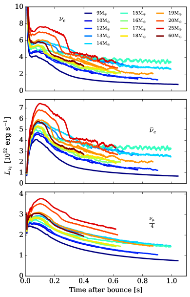
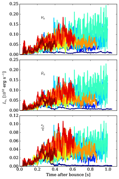
Figure 1: Left: Luminosity (in 10⁵² erg s^-1) as a function of time after bounce (in seconds)at 250 km and (right): the quadrupole components of the luminosity (in 10⁵² erg s^-1) as a function of time after bounce (s) for all three neutrino species. The higher luminosities for the electron neutrinos and anti-neutrinos for the 13-, 14-, and 15-M_⊙ progenitors result from sustained accretion for these non-exploding models. The spiral SASI is most evident for the 15-M_⊙ progenitor, which shows periodic oscillations in the neutrino luminosities after $\sim$500 ms. The non-exploding models also show large quadrupolar components at later times. However, this does not always yield a higher neutrino gravitational signal. See text for a discussion.

In Fig. 1, we plot on the left-hand side the neutrino luminosity (equivalent to $\Lambda(t)$ for each neutrino species in Eqns 1-2) as a function of time for all 3D models considered here for all three neutrino species. Lower mass models, such as the 9-M_⊙ model in particular, typically have lower neutrino luminosities and accretion rates. Absent explosion, the 13-,14-, and 15-M_⊙ models accrete for longer and evince higher neutrino luminosities at later times. The development of the spiral SASI (Blondin et al., 2003; Blondin & Shaw, 2007; Blondin, 2005; Kuroda et al., 2016) is evident for these non-exploding models through the quasi-periodic oscillations after $\sim$500 ms in their neutrino luminosities, and is most visible for the electron neutrinos ($\nu_{e}$) and anti-neutrinos ($\bar{\nu}_{e}$). We note that we see only the spiral SASI in the non-exploding models. The smaller shock stagnation radii inherently manifest in non-exploding models favor faster advective-acoustic timescales (Foglizzo 2002) that efficiently amplify SASI growth (see Scheck et al. 2008). Recent 3D simulations confirm this for non-exploding, or delayed-exploding, models (Roberts et al. 2016; Kuroda et al. 2016; Kuroda et al. 2017; Ott et al. 2018; Glas et al. 2019; Vartanyan et al. 2019a; Burrows et al. 2020; Vartanyan et al. 2019b). As indicated in Burrows et al. 2018; Vartanyan et al. 2018, 2019a; Burrows et al. 2020, the majority of our models explode within the first 300 milliseconds, precluding the development of a SASI. Prompt explosion is in large part due to the detailed microphysics of the simulation $-$ namely the inclusion of the axial-vector many-body correction to the neutrino-nucleon scattering rates $-$ and to the intrinsic density profile of the progenitors. Generally, we find that models with sharper Silicon/Oxygen interfaces produce earlier explosion owing to a favorable combination of a sustained neutrino luminosity and a drop in the accreta ram pressure. We also emphasize that the nature of explosion in these models is not absolute $-$ some models seem more explodable than others, but changes to the evolution physics, progenitor structure, or resolution could alter this conclusion.

In the right hand side of Fig. 1, we plot the quadrupolar neutrino luminosity as a function of time for all 3D models and for all three neutrino species. We use the approach outlined in Burrows et al. (2012) (see also Vartanyan et al. 2019b) to decompose the luminosity L${}_{\nu}(\theta,\phi)$ into spherical harmonic components with coefficients:

$$a_{lm}=\frac{(-1)^{|m|}}{\sqrt{4\pi(2l+1)}}\oint L_{\nu}(\theta,\phi)Y_{l}^{m}(\theta,\phi)d\Omega\,,$$ (5)

normalized such that $a_{00}=a_{0}=\langle L_{\nu}\rangle$ (the average neutrino luminosity). $a_{11}$, $a_{1{-1}}$, and $a_{10}$ correspond to the average Cartesian coordinates of the shock surface dipole $\langle x_{s}\rangle$, $\langle y_{s}\rangle$, and $\langle z_{s}\rangle$, respectively. The orthonormal harmonic basis functions are given by

$$Y_{l}^{m}(\theta,\phi)=\begin{cases}\sqrt{2}N_{l}^{m}P_{l}^{m}(\cos\theta)\cos m\phi&m>0\,,\\ N_{l}^{0}P_{l}^{0}(\cos\theta)&m=0\,,\\ \sqrt{2}N_{l}^{|m|}P_{l}^{|m|}(\cos\theta)\sin|m|\phi&m<0\,,\end{cases}$$ (6)

where

$$N_{l}^{m}=\sqrt{\frac{2l+1}{4\pi}\frac{(l-m)!}{(l+m)!}}\,,$$ (7)

$P_{l}^{m}(\cos\theta)$ are the associated Legendre polynomials, and $\theta$ and $\phi$ are the spherical coordinate angles.

We define the quadrupolar component of the neutrino luminosity as the following norm,

$$L_{\nu,\ell}=\frac{\sqrt{\sum_{m=-\ell}^{\ell}a_{\ell m}^{2}}}{a_{00}}\,,$$ (8)

where we take $\ell=2$.

The quadrupolar neutrino luminosity is at most a few percent of the total neutrino luminosity. Note that the exploding models peak at $\sim$0.5 second after bounce, after which the non-exploding models develop the largest quadrupolar components due to the onset of the spiral SASI. The weakly-exploding 9-M${\odot}$ progenitor shows the smallest asymmetry.

In Fig. 2, we show the geometric anisotropy parameter along the negative x-axis for the electron-type neutrinos for the $+$ polarization (top panel) and the $\times$ polarization (second panel from the top). The neutrino anisotropies can get as strong as several percent, in accordance with the quadropolar component of the neutrino luminosity. This is a factor of several higher than for the 3D simulations from Müller et al. (2012). Although the “heavy”-neutrinos show similar or slightly smaller geometric anisotropy parameters, they dominate the neutrino luminosity and hence the gravitational wave strain, plotted for $+$ and $\times$ polarizations in the bottom two panels, respectively, summed over all neutrino species. Note that we see a similar hierarchy between neutrino species and their spatial variation here as in Vartanyan et al. (2019b), using different formalisms for the neutrino anisotropy. The anisotropy parameters for the non-exploding models are largest for all species at late times, after $\sim$500 ms, corresponding to the development of the spiral SASI. However, a larger anisotropy parameter doesn’t directly translate into higher strains, as visible in the bottom two panels of Fig. 2, due to additive cancellation when integrating Eq. 2 over time.

The neutrino gravitational strain is approximately two orders of magnitude larger than the matter gravitational wave strain and shows secular growth with time. The neutrino strain is significantly different from the matter component (Radice et al., 2019; Morozova et al., 2018) $-$ it features weaker time variations and larger amplitudes, with more monotonic behavior with time. This reflects the fundamental differences of their origins. Gravitational waves from matter involve $\sim$0.1 M_⊙ with convective velocities of $\sim$1000 km s^-1 on convective timescales of milliseconds (Vartanyan et al., 2019a; Nagakura et al., 2020). On the other hand, neutrino luminosity contributions involve relativistic velocities and significant energy losses from the PNS. The memory effect (Braginskii & Thorne, 1987) from neutrinos, indicated as the integral over time in Eq. 2, smooths over small time-scale variations and allows cumulative growth of the neutrino strain.

We comment on the 9-M${\odot}$ progenitor, which explodes early and more isotropically than later exploding models, such as the 19- and 60-M${\odot}$ progenitors (Burrows et al., 2020). Early, spherical explosion and the cessation of accretion was associated with a weaker gravitational wave signal from matter motions. Radice et al. (2019) emphasized that accretion, and not solely PNS convection, was responsible for driving matter gravitational waves. The 9-M_⊙ is a good example of this distinction $-$ the PNS is convective at late times (Nagakura et al., 2020), but accretion has ended. Here, we further associate the cessation of accretion with a weak GW signal from neutrino anisotropies. The 9-M_⊙ progenitor has both small anisotropy parameters in Fig. 2 and small strains.

Note that all models take $\sim$100-200 ms for the neutrino anisotropy to manifest and result in a non-zero strain. This corresponds to the timescale for turbulence to develop and for the supernova shock to break spherical symmetry. Note that, unlike the matter component of gravitational waves, neutrinos do not show a prompt-convection burst shortly after bounce. However, like the matter component, there is a hiatus of $\sim$100-200 ms.

Lastly, we see large excursions from monotonic growth of the strain for several models due to the delay until fully-developed turbulence arises. Neglecting azimuthal-variations for the sake of simplicity, we can understand the strain evolution through the evolving geometry of the explosion. We take the $+$ polarization for an observer along the negative x-axis, where positive strains correspond to axial motions, and negative strains to equatorial motions (see also Kotake et al. 2009b for a 2D analogue along the equatorial plane). The 25-M${\odot}$ progenitor has a large negative strain until $\sim$400 ms post-bounce, when the model explodes. We see a corresponding positive bump in the $\alpha_{+}$ in the top panel of Fig. 2, and a positive bump in h₊ which corresponds to the deformation of the shock as it begins to expand. Additionally, the non-exploding progenitors maintain small strains until $\sim$500 ms post-bounce, when the spiral SASI develops. The 15-M_⊙ progenitor (in cyan) develops a large negative h₊ thenabouts, corresponding to an equatorial spiral SASI. Within a few hundred milliseconds, the strain becomes less negative as the spiral SASI precesses. We emphasize that this conclusion depends on the observer direction.

We illustrate the three-dimensional gravitational wave emission from neutrinos for both polarizations in Fig. 3 at 153 ms and 249 ms post-bounce for the 19-M_⊙ progenitor as a function of viewing angle. Here, colors are degenerate with the contours: hotter colors and convex surfaces indicate larger positive values of the strain, and cooler colors and concave surfaces indicate larger negative values of the strain. To emphasize the dependence on viewing-angle, we illustrate in Fig. 4 the same map of the gravitational wave-emission rotated by 180^∘ in azimuth. The prompt rise in the gravitational wave energy from matter contributions at $\sim$50 ms corresponds to prompt convection following neutrino breakout. The energy growth then stalls for $\sim$100 ms, before reaching values as high as $\sim$10⁴⁶ erg, and less than $\sim$10⁴⁴ erg for the lowest energy, for the 9-M_⊙ model. The stall time for the gravitational wave energy to ramp up indicates the timescale for turbulence to develop in the core-collapse supernova. This timescale for matter is not dissimilar for that from neutrinos: $\sim$100 ms. On the other hand, the energy in gravitational waves from neutrinos can be as high as 10⁴³ erg, and as low as 10⁴¹ erg, again for the 9-$M_{\odot}$ model. We note that these values are still increasing at the end of our simulation, as is the explosion energy, and longer 3D simulations are required to capture the asymptotic behavior. Additionally, non-exploding models have powerful gravitational wave signatures in both neutrinos and matter at late times that is associated with the development of the spiral SASI, which modulates the infalling accretion to source gravitational waves.

In Fig. 5, we show the gravitational wave energies from neutrino anisotropies on the left for all our models, and from matter on the right. Note that, although neutrinos dominate the gravitational strain by as much as two orders of magnitude, matter dominates the gravitational wave energy by as much as three orders of magnitude. This is simply because gravitational wave energy scales as the square of the product of the strain and the frequency, and the neutrino component resides at much lower frequencies (see Fig. 7), indicative of its secular evolution and the memory effect.

3.1 Frequency Dependence

In Fig. 6, we provide Fourier transforms of the neutrino luminosity for all three species, subtracting out the mean over a 30-ms running average, as a function of frequency (in Hz) for the 14-M_⊙ progenitor (left) and the 19-M_⊙ progenitor (right). All neutrino species show similar frequency behavior with a weak hierarchy in power in the order $\nu_{e}$, $\bar{\nu}_{e}$, and $\nu_{\mu}$, similar to the results in Vartanyan et al. (2019b). We see significant power at low frequencies corresponding to the longer secular timescales of order one second. The 14-M_⊙ progenitor, which does not explode, shows a significant bump in power at $\sim$150 Hz, corresponding to the development of the spiral SASI. Such a low-power component, between 100-200 Hz, has been well-identified with the SASI, which has modulation timescales of $\sim$O(10 ms) (Blondin & Shaw, 2007; Kotake et al., 2009a; Kuroda et al., 2016; Kuroda et al., 2017; Andresen et al., 2017). The exploding 19-M_⊙ progenitor has no SASI development.

In Fig. 7, we provide gravitational wave energy spectrograms (in B Hz^-1) from neutrino anisotropies of the non-exploding 14-M_⊙ progenitor (left), and the exploding 60-M_⊙ progenitor (right) as a function of time after bounce (s) and frequency (Hz). To compute the spectograms, we apply a Hann window function to the gravitational wave energy spectra and take a short time Fourier transform with a window size of 40 ms. Our sampling frequency is 1000 Hz. Note that most of the power lies below 50 Hz, with less power at higher frequencies. The spiral SASI in non-exploding models, like the 14-M_⊙ progenitor, contributes to this higher frequency power.

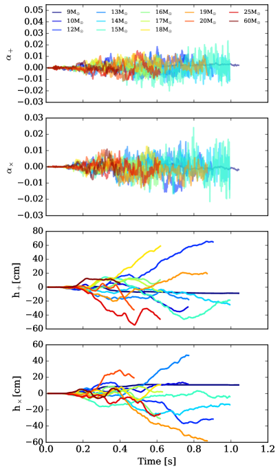
Figure 2: We show the neutrino anisotropy parameters for the electron-type neutrinos for both polarizations (top two panels), and the gravitational wave strain summed over all species of neutrinos for both polarizations (bottom panels). The values are measured along the negative x-axis.

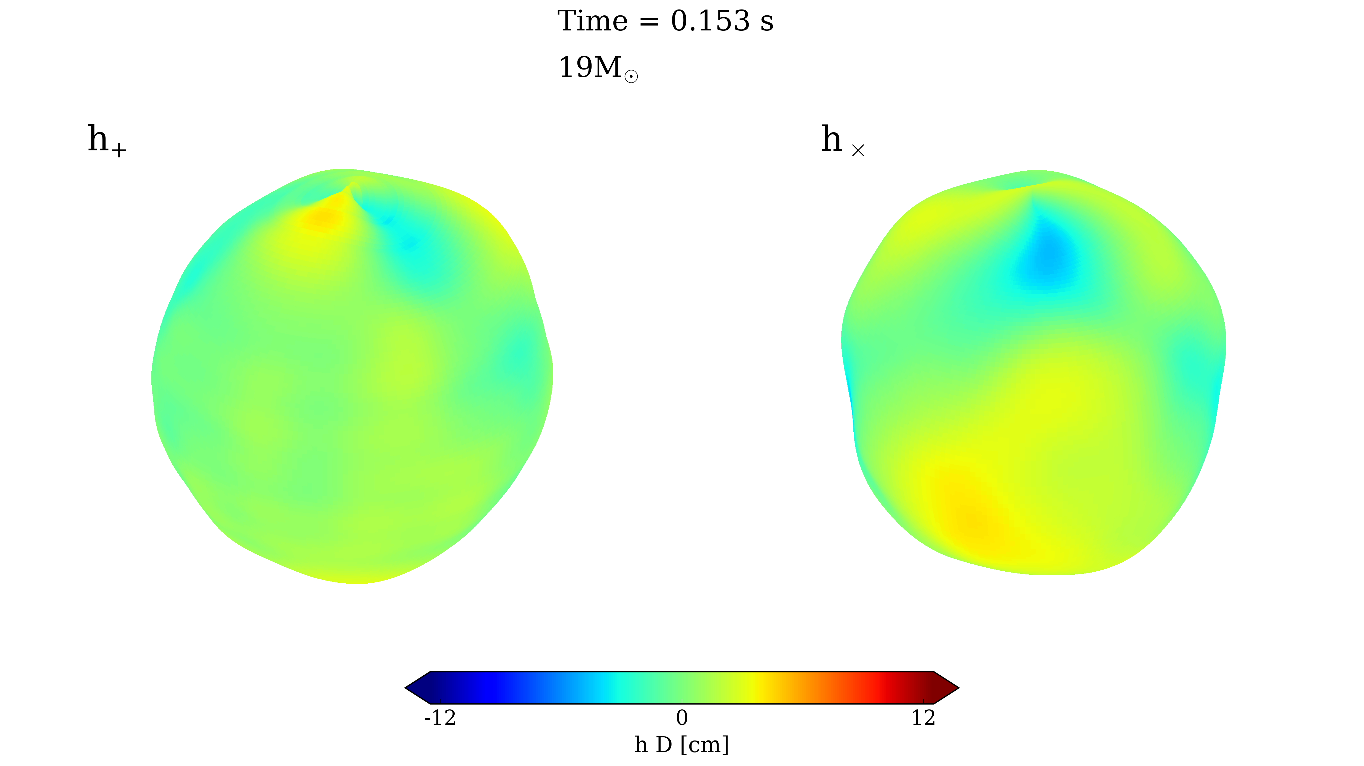
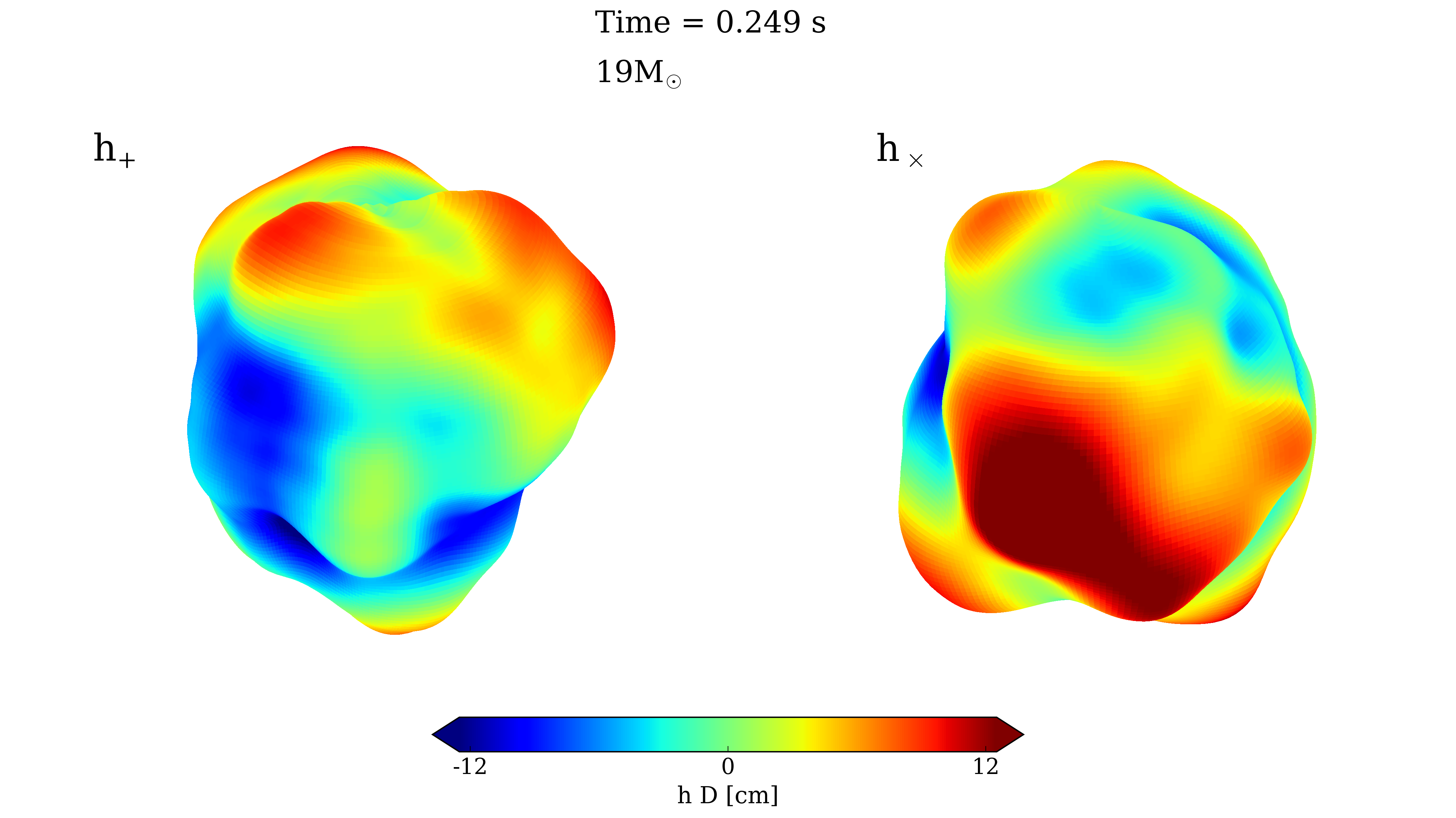
Figure 3: Three-dimensional map illustrating the gravitational-wave strain $h$ (multiplied by distance $D$) generated by neutrino emission anisotropies $253~{}\mathrm{ms}$ after bounce, assuming a stellar progenitor with mass 19-M_⊙. The signal is shown for both $h_{+}$ (left) and $h_{\times}$ (right) polarization, and as a function of the viewing angle. Hotter colors (yellow to red; convex surfaces), indicate positive strains, whereas cooler colors (blue to yellow; concave surfaces) indicate negative strains.

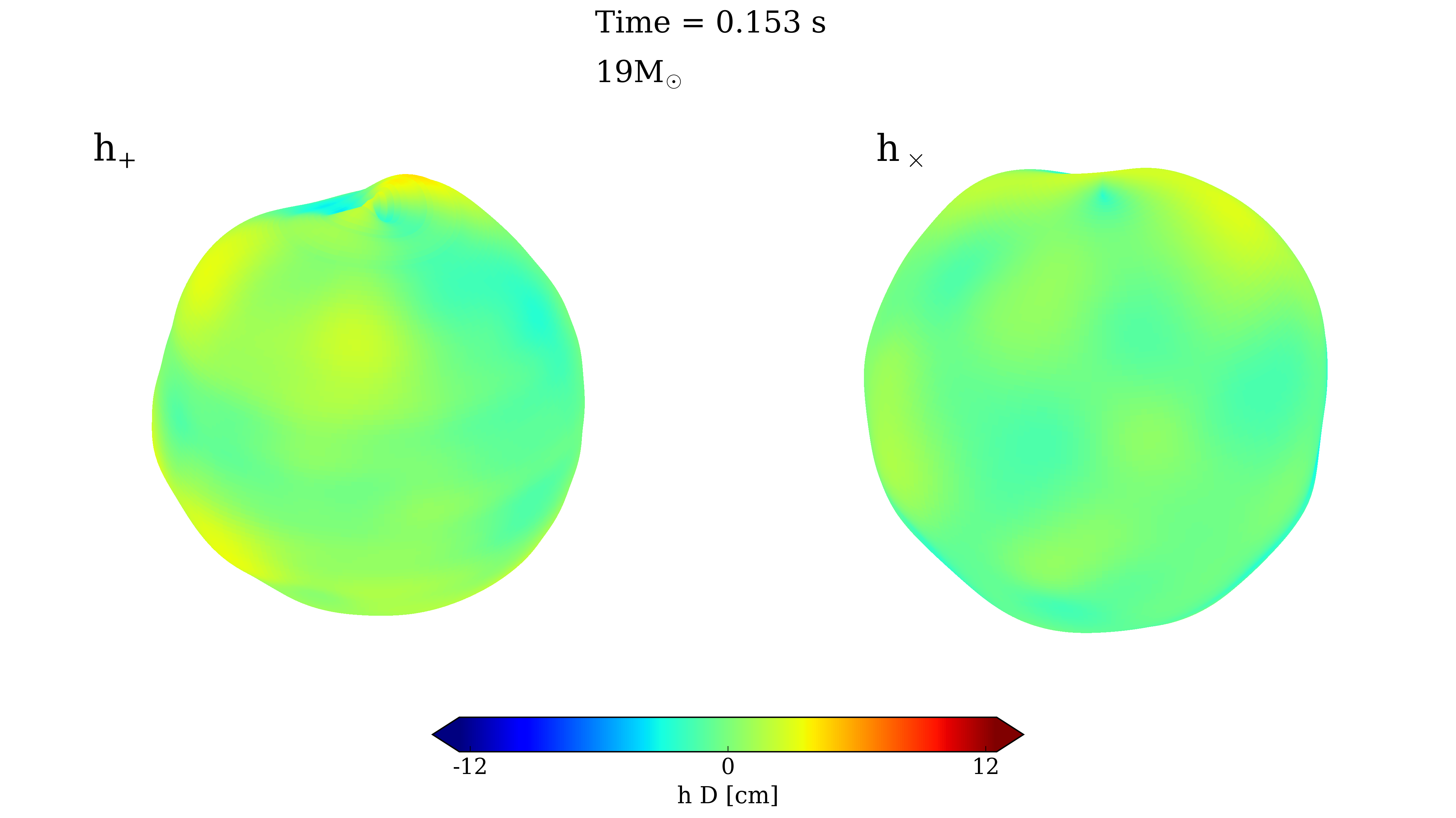
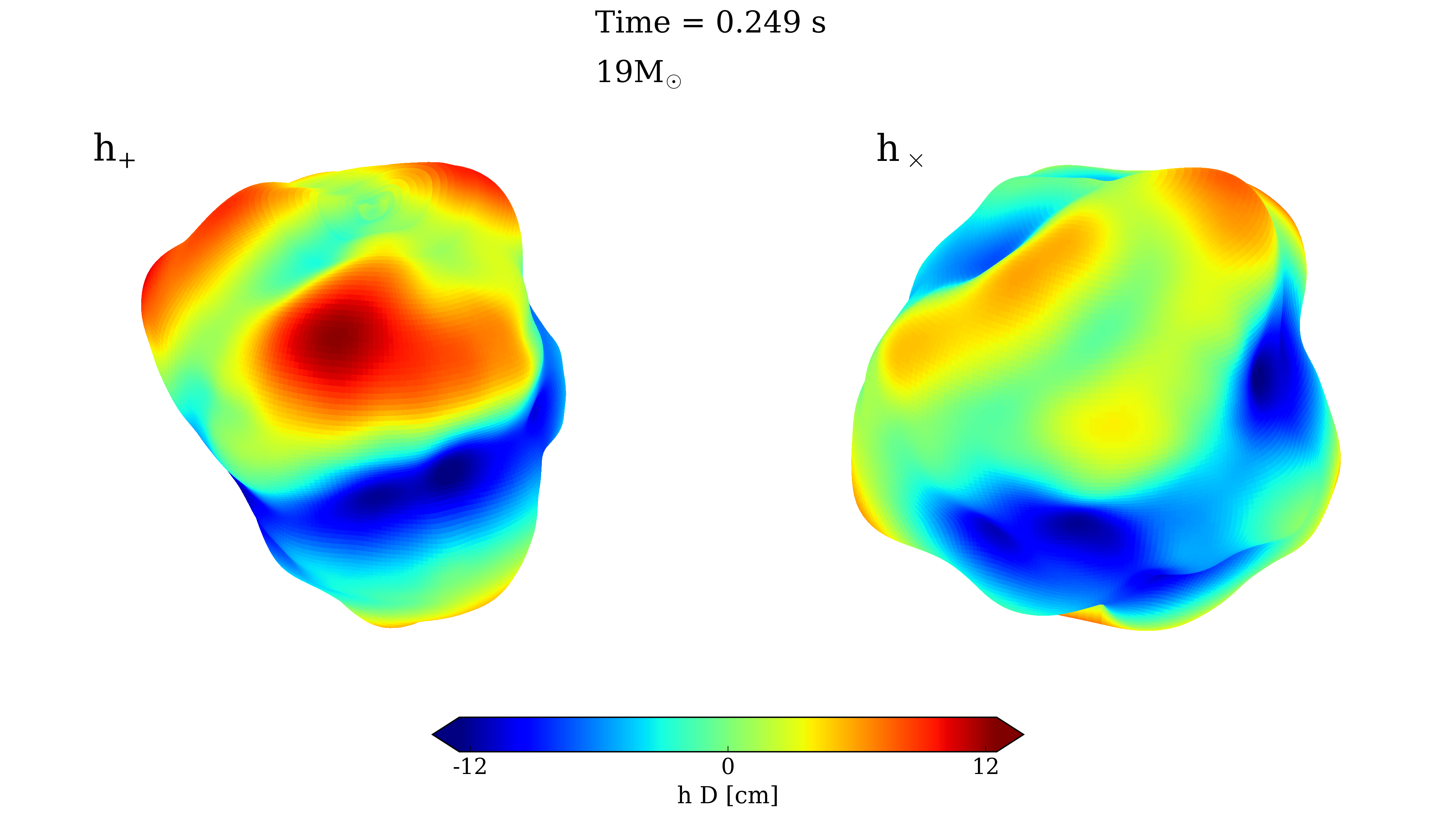
Figure 4: Same as Fig. 3, but now with the viewing angle rotated by 180^∘ along the azimuth.

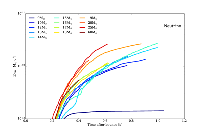
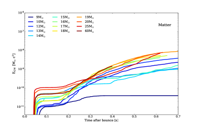
Figure 5: Here, we compare the contribution to the gravitational wave energy (in M_⊙c²) from neutrino (left) and matter (right) quadrupolar asymmetries for the various models studied in 3D as a function of time after bounce (in seconds). Note the vastly different scales on the y-axis. Neutrino contributions to the gravitational wave energies are more than three orders of magnitude smaller than those due to matter motions.

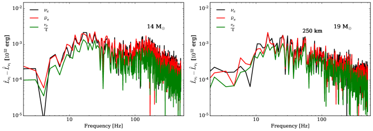
Figure 6: Fourier transform of the neutrino luminosity for all three species, subtracting out the mean over a 30-ms running average, as a function of frequency (Hz). We see significant power at low frequencies corresponding the longer secular timescales of order one second. The 14-M_⊙ progenitor (left), which does not explode, shows a significant bump in power at $\sim$150 Hz, corresponding to the development of the spiral SASI. The 19-M_⊙ progenitor (right), which does explode, is absent the SASI and the corresponding neutrino signature. Both models show also a slight bump at $\sim$300 Hz, corresponding to the timescales of small-scale convection in the PNS core.

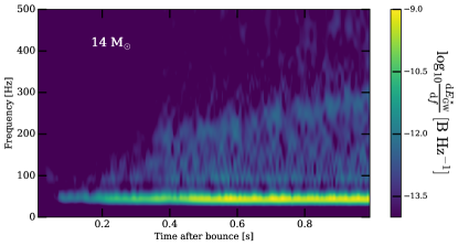
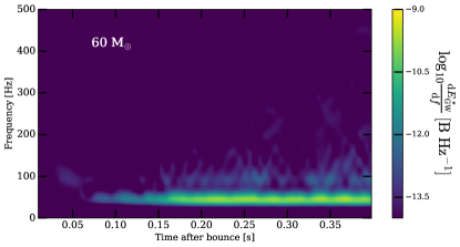
Figure 7: Gravitational wave energy spectrogram (in B Hz^-1) from neutrino anisotropies of the non-exploding 14-M_⊙ progenitor (left), and the exploding 60-M_⊙ progenitor (right) as a function of time after bounce (s) and frequency (Hz). Note that most power lies below 50 Hz, with less power at higher frequencies. The spiral SASI in non-exploding models, like the 14-M_⊙ progenitor, contributes to this power.

3.2 Detection Prospects

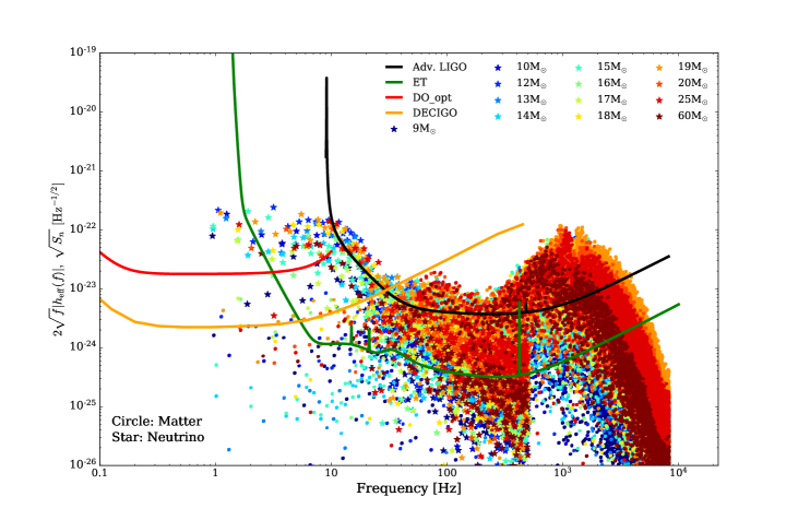
Figure 8: We plot the amplitude spectral density at 10 kpc (in Hz^-1/2) spanning $\sim$1$-$10,000 Hz for all the models studied in 3D. The neutrino component (stars) dominates from sub-Hz to several hundred Hz, whereas the matter component (circles) dominates above several hundred Hz. We also overplot the sensitivity curves for current and upcoming gravitational wave detectors. Many detectors, including aLIGO, DECIGO, and ET, will be able to detect gravitational waves from a galactic CCSN event. DO$\_$opt indicates an optimal decihertz obervatory between 2035-2050 (Arca Sedda et al., 2019) lying between LISA and ground-based detectors in frequency band designed to detect intermediate mass black hole binaries, a few $\sim 10$s to a few $\sim$100s M_⊙, with the added value of detection capabilities for galactic CCSNe.

In Fig. 8, we plot the gravitational wave amplitude spectral density at 10 kiloparsecs for all models studied in 3D, indicating both the neutrino component (stars) and matter component (circles) and compare with the sensitivity of current and proposed GW missions. Although we show the matter and neutrino components separately, in reality they combine into the net gravitational wave strain. However, as illustrated, they dominate at different frequency ranges. Above $\sim$100 Hz, the matter component dominates, peaking at 1000 Hz, corresponding to convective timescales. The neutrino component dominates below 100 Hz and plateaus below a few tens of hertz.

We overplot the sensitivity curves for three detectors: Advanced-LIGO (Zero-Det High-P design), the Einstein Telescope (design D), and DECIGO. Advanced-LIGO will be able to resolve GWs for a galactic CCSN from $\sim$ten to a few thousand Hertz (Aasi et al., 2015). The Einstein Telescope (Punturo et al., 2010; Maggiore et al., 2020), a ground-based detector with a triangle distribution of arms with baselines of ten kilometers (as opposed to four for aLIGO) will provide improved sensitivity down to one Hertz, capable of detecting even lower mass progenitors with weaker GW signals. DECIGO is a space-based heliocentric mission in the style of LISA, but with much smaller arms (1000 km) and much improved sensitivity at decihertz frequencies owing to its Fabry-Perot interfometers. We note that the high-frequency cutoff for our neutrino and matter components is simply the Nyquist frequency due to our data sampling. The lower frequency cutoff for the neutrino component is due to the length of our simulations $-$ our 3D models were carried out at most to $\sim$one second after bounce. Longer simulations will populate this lower frequency detection space. Third generation gravitational wave detectors will provide broadband coverage of galactic supernovae sensitive to both matter and neutrino asymmetries.

4 Conclusions

Recent proliferation in 3D simulation capabilities of CCSNe in the first second after bounce have additionally provided new insights into the information contained in the gravitational waves sourced by matter and in neutrino signatures. However, study of gravitational waves sourced by neutrino asymmetries has lagged. Axisymmetric 2D studies overestimate the develop of axial instabilities and of the strains in general. Additionally, simplified 3D studies, often with parametrized neutrino heating, are insufficient to study the development of neutrino asymmetries critical to understanding neutrino gravitational waveforms. Thus, 3D simulations with detailed neutrino transport are essential to study with fidelity the neutrino waveforms for CCSNe. We presented here a study of the latter, which complements matter GWs and provides new insights. The neutrino component is fundamentally different from the matter component, involving variations of relativistic radiation on secular timescales. As a result, neutrino asymmetries of only a few percent can culminate in large gravitational strains.

Despite great advances in simulation studies of CCSNe this last decade, there is still much to accomplish. In particular, the gravitational wave emissions depend on the implementation of general relativity in a supernovae code, and in Fornax we rely on a monopole approximation to relativistic gravity. In addition, improvements to the radiation transport algorithm and the neutrino microphysics will alter the neutrino heating profile of CCSNe. Moreover, higher resolution studies (e.g. Nagakura et al. 2019) may be required to capture the development of turbulence down to small scales and could result in modifications to the explosion and geometry. Lastly, longer-duration simulations, out to at least several seconds, are essential to understand the late-time asymptotic behavior of CCSNe.

In this paper, we looked at a sequence of progenitors from 9-60 M_⊙ evolved in 3D. Compared to the matter waveforms, we find that the neutrino waveforms can be up to two orders of magnitude larger in strain. Additionally, the neutrino waveform shows much less time variation and quasi-monotonic evolution due to the integral nature of the neutrino memory. However, whereas the matter component dominates at 100s to 1000s of Hertz, the neutrino component dominates at a few 10s of Hertz, and hence, contributes much less to the gravitational wave energy. Unlike the matter component, the neutrino contribution to the gravitational waveform does not have a prompt convective signal. However, both matter and neutrino GWs trace the development of turbulence in the first 100s of milliseconds after bounce.

We find an approximate trend with progenitor mass and neutrino strain strength, which probes the strength of the accretion driving turbulence that manifests the GWs and identifies both small-scale instabilities, like convection, and larger-scale instabilities like the spiral SASI. The 9-M_⊙ progenitor, with a weak and short-lived accretion history, shows the smallest neutrino asymmetries and gravitational waveforms. However models, like the 25-M_⊙, which sustain longer and more powerful accretion experience larger sustained gravitational strains.

For models that do not explode, namely the 13-, 14-, and 15-M_⊙, we find signatures of the spiral SASI in both the neutrino luminosities and the neutrino gravitational waveforms at $\sim$100 Hz, coincident with the matter gravitational waveform (Vartanyan et al., 2019b). Due to the quadrupolar nature of the strain, its sign and magnitude illustrate the geometry of explosion and indicate, for instance, the development of equatorial or axial deformations in the propagating shock front. Additionally, the strain probes the precession of the spiral SASI for non-exploding models.

Lastly, we find that neutrino GWs can be detectable for galactic events by aLIGO as well as by DECIGO and the Einstein Telescope. Future detections of gravitational waves from galactic CCSNe will explore the development of turbulence, the explosion morphology, the accretion history and the success or failure of explosion. Additionally, the low frequency gravitational waves around one Hz, will probe the secular evolution of CCSNe, longer after explosion. CCSNe emit neutrinos for many seconds after explosion, and modeling these will require carrying out 3D simulations to much longer.

References

- Aasi et al. (2015) Aasi J., et al., 2015, Classical and Quantum Gravity, 32, 074001
- Andresen et al. (2017) Andresen H., Müller B., Müller E., Janka H. T., 2017, MNRAS, 468, 2032
- Andresen et al. (2019) Andresen H., Müller E., Janka H. T., Summa A., Gill K., Zanolin M., 2019, MNRAS, 486, 2238
- Arca Sedda et al. (2019) Arca Sedda M., et al., 2019, The Missing Link in Gravitational-Wave Astronomy: Discoveries waiting in the decihertz range (arXiv:1908.11375)
- Blondin (2005) Blondin J. M., 2005, in Mezzacappa A., ed., Journal of Physics Conference Series Vol. 16, Journal of Physics Conference Series. pp 370–379, doi:10.1088/1742-6596/16/1/051
- Blondin & Shaw (2007) Blondin J. M., Shaw S., 2007, ApJ, 656, 366
- Blondin et al. (2003) Blondin J. M., Mezzacappa A., DeMarino C., 2003, ApJ, 584, 971
- Braginskii & Thorne (1987) Braginskii V. B., Thorne K. S., 1987, Nature, 327, 123
- Burrows & Hayes (1996) Burrows A., Hayes J., 1996, Phys. Rev. Lett., 76, 352
- Burrows et al. (2012) Burrows A., Dolence J. C., Murphy J. W., 2012, ApJ, 759, 5
- Burrows et al. (2018) Burrows A., Vartanyan D., Dolence J. C., Skinner M. A., Radice D., 2018, Space Science Reviews, 214, 33
- Burrows et al. (2019) Burrows A., Radice D., Vartanyan D., 2019, MNRAS, 485, 3153
- Burrows et al. (2020) Burrows A., Radice D., Vartanyan D., Nagakura H., Skinner M. A., Dolence J. C., 2020, MNRAS, 491, 2715
- Cavagliá et al. (2020) Cavagliá M., Gaudio S., Hansen T., Staats K., Szczepańczyk M., Zanolin M., 2020, Machine Learning: Science and Technology, 1, 015005
- Christodoulou (1991) Christodoulou D., 1991, Phys. Rev. Lett., 67, 1486
- Couch et al. (2020) Couch S. M., Warren M. L., O’Connor E. P., 2020, ApJ, 890, 127
- Epstein (1978) Epstein R., 1978, ApJ, 223, 1037
- Foglizzo (2002) Foglizzo T., 2002, A&A, 392, 353
- Foglizzo et al. (2012) Foglizzo T., Masset F., Guilet J., Durand G., 2012, Physical Review Letters, 108, 051103
- Glas et al. (2019) Glas R., Janka H. T., Melson T., Stockinger G., Just O., 2019, ApJ, 881, 36
- Holgado & Ricker (2019) Holgado A. M., Ricker P. M., 2019, MNRAS, 490, 5560
- Kotake (2010) Kotake K., 2010, in Journal of Physics Conference Series. p. 012011, doi:10.1088/1742-6596/229/1/012011
- Kotake et al. (2006) Kotake K., Sato K., Takahashi K., 2006, Reports on Progress in Physics, 69, 971
- Kotake et al. (2007) Kotake K., Ohnishi N., Yamada S., 2007, ApJ, 655, 406
- Kotake et al. (2009a) Kotake K., Iwakami W., Ohnishi N., Yamada S., 2009a, ApJ, 697, L133
- Kotake et al. (2009b) Kotake K., Iwakami W., Ohnishi N., Yamada S., 2009b, ApJ, 704, 951
- Kotake et al. (2011) Kotake K., Iwakami-Nakano W., Ohnishi N., 2011, ApJ, 736, 124
- Kuroda et al. (2016) Kuroda T., Kotake K., Takiwaki T., 2016, ApJ, 829, L14
- Kuroda et al. (2017) Kuroda T., Kotake K., Hayama K., Takiwaki T., 2017, ApJ, 851, 62
- Kuroda et al. (2020) Kuroda T., Arcones A., Takiwaki T., Kotake K., 2020, ApJ, 896, 102
- Li et al. (2018) Li J.-T., Fuller G. M., Kishimoto C. T., 2018, Physical Review D, 98
- Mabanta et al. (2019) Mabanta Q. A., Murphy J. W., Dolence J. C., 2019, ApJ, 887, 43
- Maggiore et al. (2020) Maggiore M., et al., 2020, Journal of Cosmology and Astroparticle Physics, 2020, 050–050
- Marek & Janka (2009) Marek A., Janka H.-T., 2009, ApJ, 694, 664
- Mezzacappa et al. (2020) Mezzacappa A., et al., 2020, Phys. Rev. D, 102, 023027
- Morozova et al. (2018) Morozova V., Radice D., Burrows A., Vartanyan D., 2018, ApJ, 861, 10
- Müller (2019a) Müller B., 2019a, Annual Review of Nuclear and Particle Science, 69
- Müller (2019b) Müller B., 2019b, MNRAS, 487, 5304
- Müller & Janka (1997) Müller E., Janka H. T., 1997, A&A, 317, 140
- Müller et al. (2012) Müller E., Janka H. T., Wongwathanarat A., 2012, A&A, 537, A63
- Müller et al. (2013) Müller B., Janka H.-T., Marek A., 2013, ApJ, 766, 43
- Müller et al. (2017) Müller B., Melson T., Heger A., Janka H.-T., 2017, MNRAS, 472, 491
- Murphy et al. (2009) Murphy J. W., Ott C. D., Burrows A., 2009, ApJ, 707, 1173
- Nagakura et al. (2019) Nagakura H., Burrows A., Radice D., Vartanyan D., 2019, MNRAS, 490, 4622
- Nagakura et al. (2020) Nagakura H., Burrows A., Radice D., Vartanyan D., 2020, MNRAS, 492, 5764
- O’Connor & Couch (2018) O’Connor E. P., Couch S. M., 2018, ApJ, 865, 81
- Ott et al. (2018) Ott C. D., Roberts L. F., da Silva Schneider A., Fedrow J. M., Haas R., Schnetter E., 2018, ApJ, 855, L3
- Powell & Müller (2019) Powell J., Müller B., 2019, MNRAS, 487, 1178
- Powell & Müller (2020) Powell J., Müller B., 2020, MNRAS, 494, 4665–4675
- Punturo et al. (2010) Punturo M., et al., 2010, Classical and Quantum Gravity, 27, 194002
- Radice et al. (2017) Radice D., Burrows A., Vartanyan D., Skinner M. A., Dolence J. C., 2017, ApJ, 850, 43
- Radice et al. (2018) Radice D., Abdikamalov E., Ott C. D., Mösta P., Couch S. M., Roberts L. F., 2018, Journal of Physics G Nuclear Physics, 45, 053003
- Radice et al. (2019) Radice D., Morozova V., Burrows A., Vartanyan D., Nagakura H., 2019, ApJ, 876, L9
- Roberts et al. (2016) Roberts L. F., Ott C. D., Haas R., O’Connor E. P., Diener P., Schnetter E., 2016, ApJ, 831, 98
- Sato et al. (2017) Sato S., et al., 2017, in Journal of Physics Conference Series. p. 012010, doi:10.1088/1742-6596/840/1/012010
- Scheck et al. (2008) Scheck L., Janka, H.-Th. Foglizzo, T. Kifonidis, K. 2008, A&A, 477, 931
- Schmitz (2020) Schmitz K., 2020, New Sensitivity Curves for Gravitational-Wave Experiments (arXiv:2002.04615)
- Seadrow et al. (2018) Seadrow S., Burrows A., Vartanyan D., Radice D., Skinner M. A., 2018, MNRAS, 480, 4710
- Skinner et al. (2019) Skinner M. A., Dolence J. C., Burrows A., Radice D., Vartanyan D., 2019, ApJS, 241, 7
- Sotani et al. (2017) Sotani H., Kuroda T., Takiwaki T., Kotake K., 2017, Phys. Rev. D, 96, 063005
- Srivastava et al. (2019) Srivastava V., Ballmer S., Brown D. A., Afle C., Burrows A., Radice D., Vartanyan D., 2019, Phys. Rev. D, 100, 043026
- Sukhbold et al. (2016) Sukhbold T., Ertl T., Woosley S. E., Brown J. M., Janka H.-T., 2016, ApJ, 821, 38
- Sukhbold et al. (2018) Sukhbold T., Woosley S. E., Heger A., 2018, ApJ, 860, 93
- Summa et al. (2018) Summa A., Janka H.-T., Melson T., Marek A., 2018, ApJ, 852, 28
- Tamborra et al. (2013) Tamborra I., Hanke F., Müller B., Janka H.-T., Raffelt G., 2013, Phys. Rev. Lett., 111, 121104
- Thorne (1992) Thorne K. S., 1992, Phys. Rev. D, 45, 520
- Torres-Forné et al. (2018) Torres-Forné A., Cerdá-Durán P., Passamonti A., Font J. A., 2018, MNRAS, 474, 5272
- Torres-Forné et al. (2019) Torres-Forné A., Cerdá-Durán P., Passamonti A., Obergaulinger M., Font J. A., 2019, MNRAS, 482, 3967
- Turner (1978) Turner M. S., 1978, Nature, 274, 565
- Vartanyan et al. (2018) Vartanyan D., Burrows A., Radice D., Skinner M. A., Dolence J., 2018, MNRAS, 477, 3091
- Vartanyan et al. (2019a) Vartanyan D., Burrows A., Radice D., Skinner M. A., Dolence J., 2019a, MNRAS, 482, 351
- Vartanyan et al. (2019b) Vartanyan D., Burrows A., Radice D., 2019b, MNRAS, 489, 2227
- Walk et al. (2019) Walk L., Tamborra I., Janka H.-T., Summa A., 2019, Phys. Rev. D, 100, 063018
- Wallace et al. (2016) Wallace J., Burrows A., Dolence J. C., 2016, ApJ, 817, 182
- Yagi & Seto (2011) Yagi K., Seto N., 2011, Phys. Rev. D, 83, 044011
- Yoshida et al. (2019) Yoshida T., Takiwaki T., Kotake K., Takahashi K., Nakamura K., Umeda H., 2019, ApJ, 881, 16