The Heart of Entanglement: Chiral, Nematic, and Incommensurate Phases in the Kitaev-Gamma Ladder in a Field

Abstract

The bond-dependent Kitaev model on the honeycomb lattice with anyonic excitations has recently attracted considerable attention. However, in solid state materials other spin interactions are present, and among such additional interactions, the off-diagonal symmetric Gamma interaction, another type of bond-dependent term, has been particularly challenging to fully understand. A minimal Kitaev-Gamma (KG) model has been investigated by various numerical techniques under a magnetic field, but definite conclusions about field-induced spin liquids remain elusive and one reason may lie in the limited sizes of the two-dimensional geometry it is possible to access numerically. We therefore focus on the KG model defined on a two-leg ladder which is much more amenable to a complete study, and determine the entire phase diagram in the presence of a magnetic field along $[111]$-direction. Due to the competition between the interactions and the field, an extremely rich phase diagram emerges with fifteen distinct phases. Focusing near the antiferromagnetic Kitaev region, we identify nine different phases solely within this region: several incommensurate magnetically ordered phases, spin nematic, and two chiral phases with enhanced entanglement. Of particular interest is a highly entangled phase with staggered chirality with zero-net flux occurring at intermediate field, which along with its companion phases outline a heart-shaped region of high entanglement, the heart of entanglement. We compare our results for the ladder with a C₃ symmetric cluster of the two-dimensional honeycomb lattice, and offer insights into possible spin liquids in the two-dimensional limit.

I Introduction

The Kitaev model on a two-dimensional honeycomb lattice is a rare example of an exactly solvable model offering a quantum spin liquid with fractional excitations.Kitaev (2006) Under a time-reversal symmetry breaking field, it exhibits non-Abelian anyons with half-quantized thermal Hall conductivity originated from Majorana edge mode. Since the original proposal, finding a solid state material possessing such a quantum spin liquid has attracted great attention. A microscopic mechanism for realizing the Kitaev model in solid-state material was first suggested using the combined effects of strong spin-orbit coupling and electron-electron interactionsKhaliullin (2005); Jackeli and Khaliullin (2009). Later, the nearest neighbor generic spin model on an ideal honeycomb lattice was re-derived, and it was found that there are additional bond-dependent interactions present with the so-called Gamma ($\Gamma$) interaction among the most intriguing.Rau et al. (2014)

From the material perspective, $\alpha$-RuCl₃ was proposed as a leading candidate with a weaker coupling between layers making the material close to two dimensional (2D).Plumb et al. (2014); Kim et al. (2015); Koitzsch et al. (2016); Sandilands et al. (2016); Zhou et al. (2016); Banerjee et al. (2016) Furthermore, the $\Gamma$ interaction has been found to be as large as the Kitaev interaction in $\alpha$-RuCl₃.Kim and Kee (2016); Janssen et al. (2017); Winter et al. (2016) Since then, RuCl₃ has been explored by several experimental and theoretical techniques.Rau et al. (2016); Winter et al. (2017); Hermanns et al. (2018); Takagi et al. (2019); Janssen and Vojta (2019) In particular, early inelastic neutron scatteringBanerjee et al. (2016) and Raman spectroscopySandilands et al. (2015) measurements have suggested a strong frustration well above the magnetic ordering temperature, indicating strong frustration which may originate from the bond-dependent Kitaev and $\Gamma$ interactions. Remarkably, a half-quantized thermal Hall conductivity was recently reported in $\alpha$-RuCl₃ in a certain range of the magnetic field Kasahara et al. (2018) when a zig-zag magnetically ordered phase is destroyed by the magnetic field.Johnson et al. (2015) Other physical quantities accessed by several experimental techniques in RuCl₃ also suggested that there is a nontrivial intermediate phase under a magnetic field which is different from a trivially polarized spin state in high field regime.Baek et al. (2017); Zheng et al. (2017); Leahy et al. (2017); Hentrich et al. (2018); Lampen-Kelley et al. (2018); Janša et al. (2018); Banerjee et al. (2018); Shi et al. (2018); Widmann et al. (2019); Sahasrabudhe et al. (2020) However, the experimental evidence for a field-induced intermediate disordered phase in RuCl₃ is still under debate.Wolter et al. (2017); Yu et al. (2018); Yamashita et al. (2020)

In parallel to the experimental progress, theoretical attempts to find nontrivial field-induced phases in extended Kitaev model have been pursued extensively. Yadav et al. (2016); Janssen et al. (2017); Chern et al. (2017); Zhu et al. (2018); Liang et al. (2018a); Gohlke et al. (2018); Nasu et al. (2018); Ronquillo et al. (2019); Liang et al. (2018b); Liu and Normand (2018); Kaib et al. (2019); Hickey and Trebst (2019); Chern et al. (2020); Lee et al. (2020); Gohlke et al. (2020) Most numerical studies are limited to either near the antiferromagnetic (AFM) Kitaev or near the ferromagnetic (FM) Kitaev region, as the exactly solvable Kitaev point offers a starting point. In particular, a minimal Kitaev-Gamma (KG) model under a $[111]$ magnetic field has been studied near FM Kitaev and AFM $\Gamma$ region relevant to RuCl₃.Gordon et al. (2019); Chern et al. (2020); Lee et al. (2020); Gohlke et al. (2020) A 24-site exact diagonalization (ED) study showed a field-revealed Kitaev spin liquid near FM Kitaev region with a finite AFM $\Gamma$ interaction, when the magnetic field is tilted away from the $[111]$-axis.Gordon et al. (2019) However, the infinite tensor product state (iTPS) found a small confined Kitaev spin liquid, and broken C₃ rotational phases are induced under the magnetic field.Lee et al. (2020) Interestingly various large unit cell magnetic orderings have been reported in the classical KG model under the magnetic field along [111]-axis.Chern et al. (2020), which are replaced by these broken rotational phases in quantum model.Gohlke et al. (2020) Whether the C₃ broken phases are quantum spin liquids or not is at present not clear and will require further studies.

Numerical studies near AFM Kitaev limit under a magnetic field have found intriguing results.Zhu et al. (2018); Gohlke et al. (2018); Hickey and Trebst (2019); Jiang et al. (2018); Zou and He (2020); Ronquillo et al. (2019); Liang et al. (2018b); Patel and Trivedi (2019); Nasu et al. (2018) It was suggested that a gapless U(1) spin liquid is induced by the magnetic field.Hickey and Trebst (2019) The energy spectra obtained by 24-site ED showed putative gapless excitations in the intermediate field, which then transition to a polarized state (PS) in high field regime. Several iDMRG studies also reported a change of central charge depending on the number of legs in the DMRG which indicates a finite spinon Fermi surface.Jiang et al. (2018) However one may question if the dense energy spectra are due to incommensurate order which is difficult to detect due to the finite size of ED and limited access to momentum points in iDMRG. Indeed, different iDMRG studies have found different gapless points in momentum space.Jiang et al. (2018); Gohlke et al. (2018); Patel and Trivedi (2019)

Despite intensive studies, definite conclusions on possible phases and the nature of numerically determined phases near the Kitaev regions remain indefinite. One reason for the controversial results among the previous studies may lie in the limited sizes of the two-dimensional honeycomb geometry that one can access numerically. Furthermore, the zero-field and field-induced phases of the entire phase space of KG model are yet to be determined. We therefore focus on the KG model defined on a two-leg ladder which is much more amenable to a detailed study and a complete phase diagram in the presence of a magnetic field along $[111]$-direction can be determined. Using high through-put iDMRG calculations we map out the entire phase diagram of the KG ladder which shows an extremely rich structure. After we determine the entire phase diagram, we focus on the region of the phase diagram where the Kitaev interaction is predominantly AFM. In this region, in the absence of a magnetic field, we identify a novel spin nematic (SN) phase with quadropolar order in addition to the AFM Kitaev phase (AK) and a phase connected to the isotropic FM ladder through a local 6-site spin rotation, FM${}_{U_{6}}$.Chaloupka and Khaliullin (2015); Kimchi and Coldea (2016); Rousochatzakis and Perkins (2018); Stavropoulos et al. (2018) In zero field the KG ladder can be mapped to a ladder with four-spin exchange closely related to JQ models Sandvik (2007) extensively studied as models of deconfined criticality Senthil et al. (2004).

When a magnetic field in the $[111]$ direction is introduced, field and spin interactions compete, and a proliferation of phases is observed. We identify phases with scalar chiral ordering and several phases with magnetic ordering some of which might display incommensurate or very large unit cell ordering. Of particular interest is two chiral ordered phases characterized by a staggered chirality (SC) and uniform chirality (UC). The SC phase is a magnetically disordered and highly entangled phase occurring at intermediate magnetic field above the AK phase. It has the staggered chirality with zero-net flux despite it is under a rather large external field, and shows clear chain end excitations. Rather poetically, this phase along with its companion phases outline a heart-shaped region of high entanglement, ‘the chiral heart of entanglement’. On the other hand, the UC phase with the uniform chirality leading to a finite net flux appears between the SN and and the rung singlet (RS${}_{U_{6}}$) phase connected to the isotropic AFM ladder through a local 6-site spin rotation.Chaloupka and Khaliullin (2015); Kimchi and Coldea (2016); Rousochatzakis and Perkins (2018); Stavropoulos et al. (2018) It emerges at extremely low field, as if three phases, SN, UC, and RS${}_{U_{6}}$ may meet at a critical point. All together, near the AFM Kitaev region alone, we identify 9 possible distinct phases in addition to the FM${}_{U_{6}}$ phase and the PS occurring at high magnetic fields.

Below, in section II, we first review the KG model. In addition to the extensive 2D cluster studies, a one-dimensional (1D) KG chain model including only $x$- and $y$-bonds was studied using non-Abelian bosonization and DMRG and reported SU(2) emergent phases.Yang et al. (2020a). The two-leg ladder is made of two such KG chains by connecting them by $z$-bond. Technical details relevant fo the iDMRG and DMRG numerical methods are subsequently discussed in the following section,  III. An overview and detailed discussion of the full phase diagram of the ladder is presented in section IV along with a discussion of the connection between the KG chain and the ladder. In section V we focus on the vicinity of the AFM Kitaev region under a magnetic field, where a rich phase diagram with various phases with enhanced entanglement is found. Finally, in section VI we compare our results for the ladder with 24-site ED results obtained in the honeycomb geometry, and discuss the implications of the ladder results to the 2D limit.

II The Two-leg Kitaev-Gamma (KG) ladder

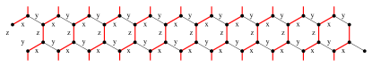
Figure 1: Two-leg ladder KG honeycomb strip with alternating $x$ and $y$ bonds along the leg and $z$-bond between the chains.

The two-leg KG ladder is formed out of a strip of the honeycomb lattice. The two KG chains with only $x$- and $y$-bonds are coupled by adding the $z$-bond as shown in Fig. 1. Periodic boundary conditions in the direction perpendicular to the ladder is then imposed by directly coupling the dangling $z$-bonds thereby forming a regular ladder. Sometimes, the additional $z$-bonds from imposing periodic boundary conditions are taken to be of opposite sign (and or strength) in which case the resulting model is usually referred to as a honeycomb ladder Karakonstantakis et al. (2013). Here, all z-bonds are identical and a regular ladder is formed. In addition to the bond-dependent Kitaev interaction, the KG Hamiltonian incorporates another bond-dependent interaction, $\Gamma$.Rau et al. (2014) For the KG ladder we orient the bonds so that the Kitaev $z$-bond connects the two legs of the ladder as shown in Fig. 1. The complete Hamiltonian is then given by

$$H_{KG}=\sum_{\langle i,j\rangle_{\gamma\in(x,y,z)}}KS_{i}^{\gamma}S_{j}^{\gamma}+\Gamma\left(S^{\alpha}_{i}S^{\beta}_{j}+S^{\beta}_{i}S^{\alpha}_{j}\right)$$ (1)

where $(\alpha,\beta)$ takes on the values $(y,z)/(x,z)/(x,y)$ for $\gamma=x/y/z$, and $\langle i,j\rangle$ refers to the nearest neighbor sites. We keep $K=\cos\phi$ and $\Gamma=\sin\phi$ and interpolate between the Kitaev ladder and $\Gamma$ ladder by varying $\phi$ from 0 to $2\pi$. We denote the total number of sites in the ladder (including both legs) by $N$. The pure Kitaev ladder at $\phi=0,\pi$ is exactly solvable Feng et al. (2007a) and at both points it is in a disordered gapped phaseFeng et al. (2007a). However, recently it was shown that a non-local string order parameter (SOP) can be defined Catuneanu et al. (2019) at the Kitaev points. The SOP remains non-zero in the presence of a small Heisenberg coupling, $J$, at both the Kitaev points. Close to the FM Kitaev point, $\phi=\pi$, the phase diagram of the KG ladder has recently been investigated in the presence of a magnetic field and additional interactions Gordon et al. (2019). On the other hand, relatively little is known about the rest of the phase diagram of the KG ladder which is our focus here.

In one dimension in the absence of a magnetic field, the closely related KG chain has been investigated in considerable detail Yang et al. (2020a, b). An extended disordered phase close to the AFM Kitaev point, $\phi=0$ has been identified along with an adjacent spin nematic phase. For the KG chain it can rigorously be established that the phase diagram is symmetric with respect to $\Gamma\to-\Gamma$, a symmetry that is clearly absent in the KG ladder.

It is of particular interest to also consider the effect of a magnetic field. Here we exclusively consider a field in the $[111]$ direction, perpendicular to the honeycomb plane of the ladder. The magnetic field leads to a Zeeman coupling as

$$H=H_{KG}-g\frac{\mu_{B}}{\hbar}\sum_{i}{\bf h}\cdot{\bf S},$$ (2)

where we choose the direction of ${\bf h}$ along the [111]-axis normalized as ${\bf h}=\frac{h}{\sqrt{3}}(1,1,1)$, $g=1$, and ${\bf S}=\hbar\frac{\sigma}{2}$ with $\sigma$ is Pauli matrix. We use units with $\hbar=1$ and $\mu_{B}=1$.

III Numerical methods

As our main tools for investigating the KG ladder we use exact diagonalization (ED), finite size density matrix renormalization group (DMRG) and infinite DMRG (iDMRG) techniques. The iDMRG calculations are performed in two different ways. A high through-put mode with a small unit cell of size 24 or 60 and a maximal bond dimension of 500 and a high precision mode with a unit cell of 60 and a maximal bond dimension of 1000. Typical precisions for the two iDMRG modes are $\epsilon=10^{-8}$ and $\epsilon=10^{-10}$, respectively, and $\epsilon=10^{-10}$ for the finite size DMRG calculations. Finite size DMRG calculations are performed both with open boundary conditions (OBC) and for smaller system sizes with periodic boundary conditions (PBC). In order to establish the phase diagram we focus on several different characteristics. With $e_{0}$ the ground-state energy per spin we define the energy susceptibilities

$$\chi_{h}^{e}=-\frac{\partial^{2}e_{0}}{\partial h^{2}},\ \ \chi_{\phi}^{e}=-\frac{\partial^{2}e_{0}}{\partial\phi^{2}},$$ (3)

where $\chi_{h}^{e}$ could equally well be called a magnetic susceptibility. For finite size systems of size $N$ it has been established Albuquerque et al. (2010) that the energy susceptibility at a quantum critical point (QCP) diverges as

$$\chi^{e}\sim N^{2/\nu-d-z}.$$ (4)

Here $\nu$ and $z$ are the correlation and dynamical critical exponents and $d$ is the dimension. It follows that $\chi^{e}$ may not necessarily detect the phase transition if the critical exponent $\nu$ is sufficiently large. We have therefore found it useful to supplement the analysis of $\chi^{e}$ by a study of the entanglement spectrum Li and Haldane (2008) (ES) at different sections of the ladder. We have found it most useful to use a partition of the ladder where a cut is introduced at site $N/2-1$ thereby intersecting a rung. With $\lambda_{\alpha}$ the eigenvalues of the resulting reduced density matrix, $\rho_{N/2-1}$ the entanglement spectrum can be defined as $-\ln\lambda_{\alpha}$ and yields a characteristic signature of a phase. Close to the QCP the $\lambda_{\alpha}$ rapidly change whereas they remain approximately constant inside a phase. We therefore focus on the largest of the $\lambda_{\alpha}$’s which we denote by $\lambda_{1}$ and study the lowest edge of the entanglement spectrum defined by

$$-\ln\lambda_{1}.$$ (5)

In a product phase $\lambda_{1}=1$ ($-\ln\lambda_{1}=0$) and such phases, with zero entanglement, are therefore easily detected by tracing out $-\ln\lambda_{1}$. Conversely, phases with high entanglement will have $-\ln\lambda_{1}\gg 0$ and of course, due to the ordering of the $\lambda_{\alpha}$ one must have $-\ln\lambda_{\alpha}>-\ln\lambda_{1}$ for any $\alpha>1$. Sometimes changes in $-\ln\lambda_{1}$ are imperceptible and we have therefore found it useful to define an entanglement spectrum susceptibility as follows

$$\chi_{h}^{\lambda_{1}}=-\frac{\partial^{2}\lambda_{1}}{\partial h^{2}},\ \ \chi_{\phi}^{\lambda_{1}}=-\frac{\partial^{2}\lambda_{1}}{\partial\phi^{2}}.$$ (6)

Since the ES has to change at the QCP, $\chi^{\lambda_{1}}$ should be able to detect any phase transition with the exception of unlikely scenario’s where $\lambda_{1}$ only changes linearly at the QCP with all non-trivial changes in the higher $\lambda_{\alpha}$’s. We have found $\chi^{\lambda_{1}}$ to be an extremely sensitive measure, often changing many orders of magnitude at a QCP, and we therefore typically focus on $\ln\chi^{\lambda_{1}}$.

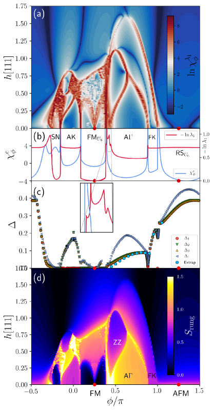
Figure 2: Phase diagram of the two-leg KG ladder model versus field, $h[111]$ and coupling $\phi/\pi$. (a) The entanglement spectrum susceptibility $\chi_{\phi}^{\lambda_{1}}$ on a logarithmic scale. (b) The energy susceptibility, $\chi_{\phi}^{e}$ (blue line) versus $\phi$ in zero field, and the lowest edge of the entanglement spectrum, $-\ln\lambda_{1}$ (red line), versus $\phi$ in zero field. (c) The excitation gap to the first 4 states, solid blue circles are extrapolations of $\Delta_{1}$ to $N=\infty$. (d) $S_{\rm rung}$ versus $\phi$ and $h[111]$. See labels in Fig. 4. Results in (a) and (d) are from high through-put iDMRG calculations with a unit cell of 60 sites with $\Delta\phi=0.01\pi,\ \Delta h[111]=0.01$ Results in (b) are from high precision iDMRG calculations with a unit cell of 60 sites with $\Delta\phi=0.001\pi$. Results in (c) are from high precision finite size DMRG calculations with PBC, $N=60$ and $\Delta\phi=0.01\pi$. Close to $\phi=\pi$ and $\phi=0.88\pi$, $\Delta\phi=0.001\pi$.

IV Full KG ladder $\phi,h[111]$ phase diagram

We start with a discussion of the full phase diagram covering the entire range $\phi\in[0,2\pi]$ and $h[111]\in[0,1.75]$. Our results for the full phase diagram as obtained from iDMRG calculations are shown in Fig. 2. We first show $\ln\chi^{\lambda_{1}}_{\phi}$ in Fig. 2(a). The divergence of $\chi^{\lambda_{1}}_{\phi}$ at a phase transition is so strong that it is most sensible to plot $\ln\chi^{\lambda_{1}}_{\phi}$. A well defined phase, where $\lambda_{1}$ is close to constant is then visible in Fig. 2(a) as a dark blue coloring. On the other hand, a divergent $\chi^{\lambda_{1}}_{\phi}$, indicating a phase transition is visible as a dark red color. As is clearly evident from Fig. 2(a) the complexity of the phase diagram due to the many competing phases is truly remarkable.

Fig. 2(b) and (c) show $\chi^{e}_{\phi}$ and $-\ln\lambda_{1}$, and the spin excitation gap at zero field, respectively. We will discuss them in detail later.

A second view of the full phase diagram is shown in Fig. 2(d) where the bipartite von Neumann entanglement entropy $S_{\mathrm{rung}}$ is shown. We define

$$S_{\mathrm{rung}}=-\mathrm{Tr}\rho_{N/2-1}\ln\rho_{N/2-1},$$ (7)

where $\rho_{N/2-1}$ is the reduced density matrix obtained from a partition of the ladder after site $N/2-1$, a partition that will cut a rung in the ladder. Highly entangled phases are here visible as bright yellow colors where as phases with negligible or no entanglement, where the ground-state wave function is well described by a simple product form, are shown as dark blue.

We note that considerable scattering are clearly visible in certain regions at finite fields, for instance above $\phi=\pi/4$ and $\phi=0$. The noise is due to poor convergence of the iDMRG due to the high frustration present. In these regions a more careful analysis with either exact diagonalizaiton or finite-size DMRG is necessary.

IV.1 Zero field phase diagram

Let us now focus on the phase diagram in zero field. A detailed high precision calculation of $\chi_{\phi}^{e}$ at zero field is shown in Fig. 2(b) along with the lower edge of the entanglement spectrum (ES), $-\ln\lambda_{1}$. A large number of well defined phase transitions are clearly visible which we now discuss.

Part of the phase diagram close to the FM Kitaev point $\phi=\pi$, has previously been discussed Gordon et al. (2019) and in zero field a gapped spin liquid phase denoted KSL between $\phi/\pi=1$ and $\phi/\pi=0.883$ along with a second gapped phase K$\Gamma$SL starting below $\phi/\pi=0.883$ have been identified. Since we here discuss the full phase diagram we shall refer to the KSL phase as FK and the K$\Gamma$SL phase as A$\Gamma$ to distinguish them from the phases ocurring at the AFM Kitaev point. The notation A$\Gamma$ makes sense since this phase surrounds $\phi=\pi/2$ where $K=0$, $\Gamma=1$.

A local unitary transformation, $U_{6}$, is also known Catuneanu (2019); Yang et al. (2020a, b). The $U_{6}$ transformation locally rotates the spins in a manner so that the $\Gamma$ couplings are transformed into Heisenberg like ($xx$, $yy$, or $zz$) couplings with a changed sign. The transformation can be applied equally well to the chain, the ladder and the honeycomb plane. At the points $\phi=\pi/4$ and $\phi=5\pi/4$ where the Kitaev and $\Gamma$ couplings are of equal strength the KG ladder is therefore transformed into an isotropic FM and AFM Heisenberg ladder. These two points therefore have hidden SU(2) symmetry. It is well established that the isotropic AFM Heisenberg ladder is in a gapped disordered rung singlet (RS) phase Dagotto et al. (1992); Barnes et al. (1993) and we therefore denote the corresponding phase for the KG ladder as RS${}_{U_{6}}$. In the two-dimensional honeycomb lattice limit the RS${}_{U_{6}}$ phase becomes a 120 degree ordered phase.Rau et al. (2014) For the FM point, $\phi=\pi/4$ we denote the magnetically ordered gapless phase by FM${}_{U_{6}}$. Since the FM${}_{U_{6}}$ is well approximated by a product wave function with negligible entanglement it is distinctly visible in Fig. 2(d) with its almost black coloring. The FM and AFM points are shown as solid red circles along the $\phi$-axis in Fig. 2. The same unitary $U_{6}$ transformation transforms the FM Kitaev point, $\phi=\pi$, to the AFM Kitaev point, $\phi=0$. The energy spectrum at these two points must therefore be identical, a property that does not hold for any non-zero $\Gamma$.

Starting from right to left we observe the transition from RS${}_{U_{6}}$ to the FK phase occurs at $\phi/\pi=1$ with the subsequent transition from the FK phase to the A$\Gamma$ phase occurring at $\phi/\pi=0.883$. Between the gapless FM${}_{U_{6}}$ phase and the gapped A$\Gamma$ phase we observe a rapid sequence of several well defined phase transitions at $\phi/\pi=0.440$, $\phi/\pi=0.428$, $\phi/\pi=0.396$ and finally at $\phi/\pi=0.385$. See the zoomed inset in Fig. 2(b). While $\chi_{\phi}^{e}$ only detects a single transition at $\phi/\pi=0.385$ the other 3 transitions are clearly identifiable in $-\ln\lambda_{1}$ as shown in the zoomed inset. The precise nature of the intervening phase is at present unclear and left for future study. A clear transition out of the FM${}_{U_{6}}$ phase to the gapped spin liquid phase AK is observed at $\phi/\pi=0.086$. As previously mentioned, precisely at $\phi=0$ a non-local string order has been found Catuneanu et al. (2019) and the AK phase is clearly identifiable as a spin liquid phase. In the 2D honeycomb lattice limit the AK phase becomes the AFM Kitaev spin liquid. We shall discuss the AK phase further below. We now turn to a discussion of the last phase observed in zero field, to the left of the AK phase.

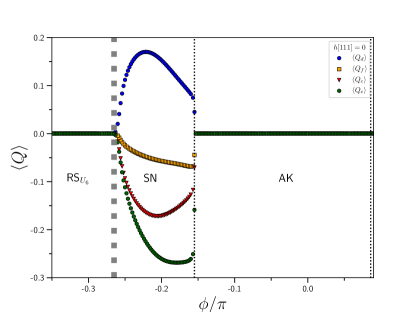
Figure 3: Nematic ordering at zero field in the AFM Kitaev region. The nematic order parameters are determined along one leg of the KG ladder. Results are from high precision iDMRG calculations with a unit cell of 60. The dotted vertical lines denote the transitions at critical fields determined from divergences in $\chi_{\phi}^{e}$ and $\chi_{\phi}^{\lambda_{1}}$.

IV.1.1 Nematic Phase in zero Field, SN

In a recent study Yang et al. (2020b) the KG chain was investigated and a phase with spin-nematic (spin-quadropole) order adjacent to the spin-liquid phase at $\phi=0$ was identified. From a symmetry analysis of the following 4 order parameters were identified:

$$Q_{c} = S^{x}_{j}S^{y}_{j+1}+S^{y}_{j}S^{x}_{j+1}$$

$$Q_{d} = S^{x}_{2n+1}S^{z}_{2n+2}+S^{z}_{2n+1}S^{x}_{2n+2}+$$

$$S^{y}_{2n+2}S^{z}_{2n+3}+S^{z}_{2n+2}S^{y}_{2n+3},\ \ n=0,1,\ldots$$

$$Q_{e} = S^{y}_{2n+1}S^{y}_{2n+2}+S^{x}_{2n+2}S^{x}_{2n+3},\ \ n=0,1,\ldots$$

$$Q_{f} = S^{z}_{j}S^{z}_{j+1}$$

The two order parameters $Q_{c}$ and $Q_{d}$ describe off-diagonal ordering between sites not coupled by the same terms in the Hamiltonian and $Q_{e}$, $Q_{f}$ diagonal ordering again between sites not coupled the same way in the Hamiltonian. The above definitions therefore depend on a specific ordering of the couplings along the leg. Considering only the Kitaev coupling, site 1,2 would be $xx$ coupled, site 2,3 $yy$ coupled and so forth. (Note that along the legs of the KG ladder no $S^{z}S^{z}$ coupling occurs so $Q_{f}$ can be defined between any two nearest neighbor sites). We can use the same order parameters to study nematic ordering along the legs of the KG ladder. Our results are shown in Fig. 3 as obtained from iDMRG. Due to the translational invariance the $Q$’s are the same among all sites and are easily calculated. They all four become non-zero at $\phi/\pi=-0.155$ which coincides with divergences in $\chi_{\phi}^{e}$ and $\chi_{\phi}^{\lambda_{1}}$. The transition by varying $\phi$ is also clearly visible directly in $-\ln\lambda_{1}$ as can be seen in Fig. 2(b).

However, this is not a conventional spin-quadropole phase. The DRMG with OBC shows two different magnetic orderings depending on the size of the system. One has the AFM order along the leg and FM between the rung, and the other has a 6-site ordering mapping to AFM order after 6-site transformation, while the iDMRG finds the first one. The AFM order corresponds to a stripe order, if we continue the ordering pattern by increasing the number of ladders to the the 2D limit. Let us briefly consider what happens if an additional Heisenberg coupling $J$ is introduced along side the $K$ and $\Gamma$ terms. In that case, the striped phase appears for an AF Heisenberg interaction $J>0$ in 24-site ED calculations on the C₃ cluster, while the second ordering is likely a spiral order occurring for $J<0$.Rau et al. (2014) This suggests that this particular window of $\phi$ with $J=0$ is in fact a line of first order transitions (in $J$) between these two orderings. To confirm such a possibility, we have studied the phase boundary by sweeping $J$ ( parameterized as $J\equiv K\cos\theta)$. Indeed we find a clear first order transition occuring at $J=0$ in $\chi_{\theta}^{e}$, the second derivative of ground state energy per spin with respect to $\theta$, as shown Appendix B.

While it is a line of first order transitions, we would refer to this as SN for spin-nematic, as the SN is a common feature of these orderings coexiting along the transition line. As the magnetic field becomes finite, it develops a magnetic order with almost zero entanglement which is shown later. The transition out of the SN phase into the RS${}_{U_{6}}$ phase occurs at around $\phi/\pi=-0.265$. As we shall discuss later, this quantum phase transition is actually a multi-critical point where the first order transition line ends, and two other phases occur. A high precision determination of the location of the critical point is therefore significantly more difficult than for the other QCP’s. In particular so, since the entanglement for $\phi<$$\phi/\pi=-0.265$ is exceedingly high. It is therefore shown as a broader dashed line in Fig. 3.

IV.1.2 Excitation gap in Zero field

In Fig. 2(c) we show the spin excitation gap to the first 4 lowest lying states, $\Delta_{1}$, $\Delta_{2}$, $\Delta_{3}$ and $\Delta_{4}$ as obtained from high precision finite size DMRG on ladders with $N=60$. We have verified that finite size effects are relatively small if not in the proximity of a QCP. This is indicated by the solid blue circles in Fig. 2(c) which indicate extrapolations to $N=\infty$ of $\delta_{1}$ by fitting data for $N=24,36,48,60$ and $72$ to the form $\Delta(L)=\Delta_{\infty}+a\exp(-L/\xi)/L$.

Starting from the right, we find that the RS${}_{U_{6}}$ phase, as expected, has a single ground-state with a well defined triplet excitation through-out most of the phase. The triplet excitation merges with higher lying excitations at $\phi=1.56\pi$. Precisely at the FM Kitaev point, $\phi=\pi$, there is a level crossing leading to a clear first order transition. This is exact also for finite systems. The same holds true by symmetry at the AFM Kitaev point $\phi=0$. However, while the FK phase has a single ground-state below a well defined gap and $\phi=\pi$ is a transition point, in the AK phase the ground-state remains double degenerate below a gap, only split by finite-size effects. The A$\Gamma$ phase also has a single ground state with a well defined triplet excitations above it. The FM${}_{U_{6}}$ phase is gapless, but occasionally excited state DMRG calculations get trapped in higher lying states and the gapless nature of the phase does not appear clearly in Fig. 2(c). The final phase we discuss here, the SN phase occurring between $\phi/\pi=-0.265$ and $\phi/\pi=-0.155$ is clearly gapless as can be seen in Fig. 2(c) with all four gaps close to zero.

IV.2 Relation to 1D KG Chain

As eluded to above, the phase diagram of the ladder is closely connected to that of the KG chain and the KG model defined on the full two-dimensional honeycomb lattice.

Comparing to the phase diagram of the KG chain Yang et al. (2020a, b), a gapped FK phase appeared in the ladder, while it was gapless in the chain model. Similarly, the AK persists near AFM Kitaev region, and it is gapped in the ladder, while gapless in the chain. RS${}_{U_{6}}$ is gapped in the ladder similar to AFM Heisenberg model, where as it was gapless in the chain. FM${}_{U_{6}}$ remains magnetically ordered with gapless excitations as was the case for the chain. For the chain a gapless nematic phase was identified Yang et al. (2020b) on either side of the AK phase. For the ladder a similar gapless phase, SN, occurs but this time only on one side of the AK phase. A$\Gamma$ remains disordered like the chain. There is therefore a close connection between the phases identified in the KG chain but we expect the KG ladder to be much closer to the two-dimensional honeycomb lattice and to represent most of the phases occurring in that limit although we in some cases expect phases to become gapless in the two-dimensional limit. For instance, in the KG ladder AK and FK phases are gapped and we expect these phases to become the AFM and FM Kitaev spin liquid, respectively in the 2D limit, which are gapless.

IV.3 Non-zero Field

When a magnetic field in the [111] direction is introduced, the full $h[111]$, $\phi$ phase diagram is revealed as shown in Fig. 2(a) and (d). From the rung entanglement, $S_{\mathrm{rung}}$, shown in Fig. 2(d), it is clear that the introduction of a field in many cases tend to increase the entanglement. New highly entangled phases appear until the fully field polarized state is attained where all spins are polarized along $h[111]$. We denote this polarized state by PS. Trivially, it is a product state with zero entanglement. We start by discussing the fate of the RS${}_{U_{6}}$ phase. This phase is adiabatically connected to the PS phase and no phase transition is observed at any non-zero field strength. This is contrary to the FM${}_{U_{6}}$ phase state which cannot be adiabatically connected to the PS phase. This follows from the fact that the phase is not an ordinary FM state but only related to one through the local unitary rotation $U_{6}$. An alignment of the spins along the [111] direction is therefore energetically costly. As can be seen in Fig. 2(a) and (d) a line of phase transitions around field strengths of $h[111]=0.7-1.0$ occur, signalling the transition to the PS phase. A new phase at finite field above $\phi=\pi/2$ is clearly visible. This is a gapless, magnetically ordered phase with the spins arranged in a zig-zag manner, in opposite directions on the two legs of the ladder, and we refer to this phase as the ZZ phase. The fate of the phases occurring between $\phi/\pi=0.440$ and $\phi/\pi=0.385$ is not known and left for future study. The FK and A$\Gamma$ phases survive in the presence of a magnetic field and survive up to large field strengths. The nature of these two phases in the presence of $h[111]$ has previously been discussed Gordon et al. (2019). We therefore leave that part of the phase diagram aside an instead concentrate on the part of the phase diagram close to the AFM Kitaev point, $\phi=0$.

In the vicinity of $\phi=0$ it is clear from Fig. 2(a) and (d) that several new phase are induced by the magnetic field, in many cases with significantly increased entanglement. The nematic phase, SN, identified in zero field, survive in the presence of a non-zero field and is clearly visible in Fig. 2(a) and (d). However, the high through-put iDMRG calculations used in Fig. 2 are in certain regions having trouble achieving convergence as can be seen by the noise in the figure and a precise determination of the phase diagram in the vicinity of $\phi=0$ is difficult from the data presented in Fig. 2(a) and (d). We therefore focus on a high resolution study of that part of the phase diagram combined with finite-size DMRG calculations for the regions where it is not possible to achieve good convergence using iDMRG.

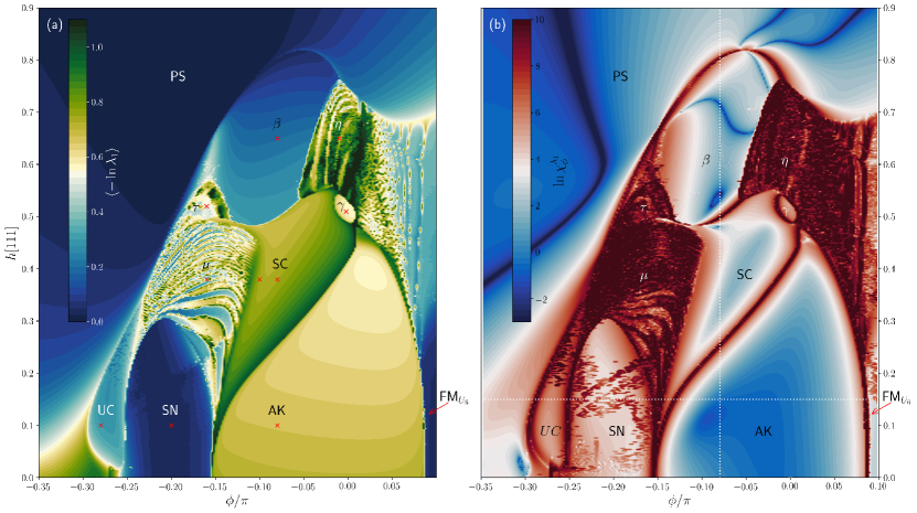
Figure 4: Phase diagram for the AFM Kitaev region of the two-leg ladder KG ladder model under the magnetic field along [111]-axis. (a) Lowest edge of the entanglement spectrum, $-\ln\lambda_{1}$ of the reduced density matrix, $\rho_{L/2-1}$, versus $\phi$ in zero field. Dark blue corresponds to $\lambda_{1}=1(-\ln\lambda_{1}=0)$ a phase of low entanglement and close to a product state. Dark green corresponds to a small $\lambda_{1}$ and higher entanglement. The $\times$’s corresponds to points studied in detail in Fig. 5, 6. (b) The entanglement spectrum susceptibility $\chi_{\phi}^{\lambda_{1}}$ on a logarithmic scale. Deep blue coloring corresponds to a stable $\lambda_{1}$ a well defined phase, dark red coloring signals rapid change in $\lambda_{1}$ and a likely associated phase transition. The dashed lines are studied in Fig. 8, 9. Identical phase diagrams obtained from $\chi_{h}^{e}$ and $S_{\mathrm{rung}}$ can be found Appendix A. All results in (a) and (b) are from high throughput iDMRG calculations with a unit cell of 24 sites, with $\Delta\phi=0.002\pi,\ \Delta h[111]=0.002$.

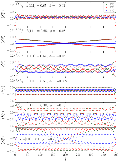
Figure 5: On-site magnetization $\langle S_{i}^{\alpha}\rangle$, $\alpha=x$ (green), $y$ (red) and $z$ (blue) along the ladder at six different points in the phase diagram indicated in Fig. 2 representing the (a) $\eta$, (b) $\beta$, (c) $\tau$, (d) $\gamma$, (e) $\mu$ and (f) SN phases. Results are from finite-size DMRG calculations for total system size $N=400$ with open boundary conditions. For clarity, results are shown only for one leg of the ladder.

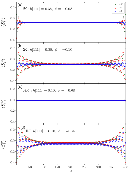
Figure 6: On-site magnetization $\langle S_{i}^{\alpha}\rangle$, $\alpha=x$ (green), $y$ (red) and $z$ (blue) along the ladder at four different points in the phase diagram indicated in Fig. 2 representing the (a) SC-phase at $h[111]=0.38$, $\phi=-0.08\pi$, (b) SC-phase at $h[111]=0.38$, $\phi=-0.10\pi$, (c) AK-phase and (d) UC phase. Results are from finite-size DMRG calculations for total system size $N=400$ with open boundary conditions. For clarity, results are shown only for one leg of the ladder.

V The Antiferromagnetic Kitaev Region, $|\Gamma|\ll K$

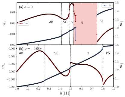
Figure 7: Magnetization versus field, $h[111]$. (a) $m_{\perp}$ (red circles) and $m_{\parallel}$ (blue circles) versus $h[111]$ at the AFM Kitaev point $\phi=0$. (b) $m_{\parallel}$ (red circles) and $m_{\perp}$ (blue circles) versus $h[111]$ (blue circles) near the AFM Kitaev point $\phi=-0.08\pi$. Results in (a), (b) are from high precision iDMRG calculations with a unit cell of 60 performed at $\phi=-0.08\pi$. The dotted vertical lines denote the transitions at critical fields determined from divergences in $\chi_{h}^{e}$ and $\chi_{h}^{\lambda_{1}}$. Note that, $m_{\parallel}$ is roughly 2 orders of magnitude larger than $m_{\perp}$.

The most exotic part of the phase diagram of the KG model under the field is the AFM Kitaev region around $\phi=0$ where $|\Gamma|\ll K$. In zero field we have identified the AK spin liquid phase and the nematic phase SN. However, it is clear that there is a very fine balance among the different couplings and the presence of a magnetic field will substantially increase this competition. We therefore investigate this part of the phase diagram with extreme care. Our results are presented below.

In order to get a detailed picture of the phase diagram we have performed high through-put iDMRG calculations in the region $\phi\in[-0.35,0.10]$ and $h[111]\in[0.00,1.75]$ on a grid with $\Delta\phi=0.002\pi,\ \Delta h[111]=0.002$ using 24 site unit cells. By necessity, we have to use a relatively small unit cell and a maximal bond dimension of 500. Our results are shown in Fig. 4. In panel (a) is shown the lower edge of the entanglement spectrum, $-\ln\lambda_{1}$, determined from the reduced density matrix that cuts a rung. Phases with negligible entanglement ($\lambda_{1}\sim 1)$ will show as dark blue where as highly entangled phases ($\lambda_{1}\ll 1)$ are colored yellow to dark green. The AK phase is clearly visible as the bright yellow phase centered around $\phi=0$, extending to non-zero fields. On the other hand, the SN phase which is close to a product state is clearly visible as dark blue. In addition to these two previously discussed phases there is a proliferation of phases occurring at higher fields. In order to more clearly identify phase transitions we show $\chi_{\phi}^{\lambda_{1}}$ in Fig. 4(b) on a logarithmic scale. Deep blue coloring in Fig. 4(b) corresponds to a stable $\lambda_{1}$, a well defined phase, while dark red coloring signals rapid change in $\lambda_{1}$ and a likely associated phase transition. Note the logarithmic scale, where the darkest red coloring is more than 10 orders of magnitude larger than the blue colors. A significant advantage analyzing the phase diagram in the way shown in Fig. 4(a) and (b), is that the entanglement spectrum, and therefore also $\lambda_{1}$, has to change at a quantum phase transition.

In Fig. 4(b) many clear phase transitions are visible as dark red lines. However, there are also some extended regions with dark red coloring or noise appearing. These regions marked, $\eta,\tau$ and $\mu$ in Fig. 4(a), (b), are regions where the small unit cell idmrg calculations have difficulty reaching good convergence. Likely this is due to incommensurability effects and a further investigation using finite size DMRG or ED is warranted. From the data in Fig. 4(a), (b) we identify six well defined phases, the previously discussed AK and SN phases and 4 new phases that we name SC, $\beta$, $\gamma$ and UC. Here SC and UC refer staggered chirality (SC) and uniform chirality (UC) because these phases exhibit a staggered and uniform pattern of chirality without any magnetic ordering, respectively. As we discuss in more detail below, it appears that the $\mu$ region is distinct from the SC phase and it seems quite plausible that the $\eta,\tau$ and $\mu$ regions are in fact well-defined phases and we therefore discuss them as such below. However, at present we cannot exclude the possibility that, for instance, what appears as a phase transition between the SN phase and the $\mu$ phase is instead a ‘disorder’ line marking the onset of incommensurate short range correlations thereby hindering the convergence of the iDMRG calculations. It is therefore possible that the $\eta,\tau$ and $\mu$ regions are not distinct phases but simply parts of the adjoining phases where short-range correlations are different. We shall return to this point below. Surprisingly, it is clear that some of the phases occurring at finite field have significantly increased entanglement, most notably the SC phase that together with its accompanying phases, $\gamma$ and $\mu$ outline a heart shaped region of extraordinary high entanglement.

Complementary views of the same phase diagram as obtained from $S_{\mathrm{rung}}$ and $\chi_{h}^{e}$ can be found in Appendix A.

V.1 Overview of phases, $\langle S^{\alpha}_{i}\rangle$

Several of the phases visible in Fig. 4(a) and (b) are magnetically ordered phases. We have therefore performed high precision finite size DMRG calculations with $N=400$ and OBC at the points marked with a red $\times$ in Fig.. 4(a). Results for the local magnetization $\langle S^{\alpha}_{i}\rangle$ are shown in Fig. 5 and 6, here the green circles are $S^{x}_{i}$, the red circles $S^{y}_{i}$ and the blue circles $S^{z}_{i}$ along a single leg of the ladder. In some cases we find magnetic ordering with a surprisingly large unit cell, in other cases indications of incommensurate ordering. Note that a simple polarization of the spins along the field direction $h[111]$ would have all $S^{\alpha}_{i}$ equal. Before a more detailed discussion of some of the phases we summarize some of the main findings in Fig. 5 and 6.

V.1.1 Magnetically ordered phases

We start with the six phases that show clear signs of ordering.

• $\eta$: This is a high field phase (region). As shown in Fig. 5(a) the local magnetization appear incommensurate. The ground-state is degenerate and the phase is likely gapless.

• $\beta$: As $\Gamma$ is made slightly more negative the system transitions from the $\eta$ phase to the $\beta$ phase. The local ground-state magnetization along the leg of the ladder, shown in Fig. 5(b), displays a characteristic Möbius form, showing a single twist in $S^{x}_{i}$ and $S^{y}_{i}$ from one end of the open chain to the other while $S^{z}_{i}$ remains constant. The ground-state is degenerate and the phase is possibly gapless.

• $\tau$: This phase (region) is adjacent to the $\beta$ phase but the beautiful intricate ordering along the leg shown in Fig. 5(c) is clearly distinct from that observed in the $\beta$ phase with a large variation in $S^{z}_{i}$ along the leg. The unit cell for the ordering appears at this value of $\Gamma$ to be approximately 20 lattice spacings along the ladder leg. Again we find a degenerate ground-state and a possible gapless phase. At neighboring values of $\Gamma$ we find similar large unit cell ordering.

• $\gamma$: The $\gamma$ phase is nested in between the SC and $\beta$ phases occupying a small oval region around $\phi=0$, $h[111]=0.5$. The $\gamma$ phase again show an exquisite ordering along the ladder leg as shown in Fig. 5(d), in this case with a smaller unit cell of 5 lattice spacings. There is no variation in the ordering throughout the $\gamma$ phase. The ground-state is degenerate and the phase is possibly gapless. However, the bipartite entanglement entropy $S(x)$ is close to constant throughout most of the ladder which would suggest a gapped phase (see Appendix C).

• $\mu$: This phase (region) is nested above the SN phase. The magnetic ordering is shown in Fig. 5(e), in this case with a unit cell of 13 lattice spacings along the leg of the ladder. Neighboring values of $\gamma$ show variations in the local magnetization pattern and it is not clear to what extent this phase is different from the $\tau$ phase. For the $\mu$ phase we again find a degenerate ground-state and possibly a gapless phase.

• SN: In zero field the SN was clearly identified. There is no indication of a phase transition as the $h[111]$ is introduced and we therefore assume that the well defined uniform phase visible in Fig. 4(a) and (b) is adiabatically connected to the SN phase in zero field. The phase is gapless and the presence of the non-zero magnetic field induces an incommensurate local magnetization as shown in Fig. 5(f).

As outlined above, the large unit cell ordering occurring in the $\mu$ and $\tau$ phases (regions) varies with $\Gamma$ and $h[111]$. The same effect is observed for the incommensurate ordering in the $\eta$ phase. In fact, the stripes occurring in these phases visible in Fig. 4(a) are likely caused by the variations in the local ordering best compatible with the 24 site unit cell. The lines could therefore represent lock in transitions.

These phases are therefore not uniform in a conventional sense but could possibly be a series of phases with shifting sizes of unit cells for the magnetic ordering. We have not been able to resolve this.

V.1.2 Non magnetic phases

We now turn to a discussion of the three remaining disordered phases which do not show any conventional local magnetic ordering apart from that induced by the magnetic field.

• SC: In Fig. 6(a) and (b) is shown the local magnetization in the SC phase at two different values of $\phi$ both at $h[111]=0.38$. In the middle of the chain the local magnetization aligns with the $h[111]$ field and the phase is best described as disordered. Clear excitations at the end of the open chain are visible. As $\phi$ is increased from -0.08 to -0.10 approaching the $\mu$ phase the size of the chain end excitations visibly grow. The SC phase is highly entangled, significanly more so than the AK phase. The ground-state does not appear degenerate but at $h[111]=0.38$, $\phi=-0.05$ we can limit the gap to the first excited state by $\Delta_{1}<0.019$. The gap is likely smaller in other parts of the phase. The bipartite entanglement entropy $S(x)$ is close to constant throughout most of the ladder which is also consistent with a gapped phase (see Appendix C). The phase show signs of scalar chiral ordering as we discuss in more detail below.

• AK: This is the AFM Kitaev phase previously discussed. As shown in In Fig. 6(b) the local magnetization is aligned with the $h[111]$ field and only faint signs of chain end excitations are visible. The phase has a gap and in zero field a two fold degenerate ground-state. It is possible to define a string order parameter (SOP) Catuneanu et al. (2019) as we discuss below.

• UC: On the left side of the SN phase a new phase appears in the presence of a $h[111]$ field. As we shall discuss below this phase has scalar chiral ordering. The ground-state is degenerate and the phase is possibly gapless. However, the bipartite entanglement entropy $S(x)$ is close to constant throughout most of the ladder which would suggest a gapped phase (see Appendix C).

V.1.3 Total magnetization, $m_{\perp}$ and $m_{\parallel}$

It is useful to analyze the total magnetization of the open chain by separating the components parallel, $m_{\parallel}$, and perpendicular, $m_{\perp}$, to the $[111]$ field direction. We define $s^{\alpha}=\sum_{i}s^{\alpha}_{i}/N$ and then

$$m_{\parallel}=(s^{x}+s^{y}+s^{z})/\sqrt{3}$$ (9)

It follows that

$$\vec{m}_{\perp}=\vec{s}-m_{\parallel}(1,1,1)/\sqrt{3}.$$ (10)

To facilitate visualization it is most convenient to plot $|m_{\perp}|$ with a sign that we determine as $\mathrm{sign}(m_{\perp}\cdot\hat{a})$ with $\hat{a}=(1,1,-2)/\sqrt{6}$. Surprisingly, $m_{\perp}$ is completely aligned or anti-aligned with $\hat{a}$ for the two cases we shall now discuss and the angle $m_{\perp}$ forms with $\hat{a}$ in the $\hat{a}$, $\hat{b}$ plane is either 0 or $\pi$. Our results are shown in Fig. 7(a),(b) for $\phi=0$ and $\phi=-0.08\pi$, respectively. The results are from high precision iDMRG calculations with a unit cell of 60 and a maximal bond dimension of 1,000. An important point to notice in Fig. 7 is that $m_{\perp}$ is 2-3 orders of magnitude smaller than $m_{\parallel}$.

Let us first discuss the results shown in Fig. 7(a) obtained from a field sweep from 0 to 0.9 at $\phi=0$. As the $\eta$ phase is entered the iDMRG calculations fail to converge and that part of the plot is therefore colored lightly red. Starting from zero field $m_{\parallel}$ (blue circles) is found to approximately linearly increase with $h[111]$ until the SC phase is reached where a kink in $m_{\parallel}$ is observed, consistent with a divergence of $\chi_{h}^{e}$. Through the SC phase $m_{\parallel}$ increase more rapidly, this phase is therefore ’softer’, consistent with the large chain end excitations shown in Fig. 6(a),(b). A second kink in $m_{\parallel}$ is observed as the $\gamma$ phase is entered but the increase in $m_{\parallel}$ through out the $\gamma$ phase is less pronounced. As the $\eta$ phase is entered and excited kinks in $m_{\parallel}$ are again observed and in the PS phase the $m_{\parallel}$ tend toward the fully polarized value of 1/2. On the other hand $m_{\perp}$ (red circles) is non monotonic throughout the AK phase, approaches small values in the SC phase before jumping to larger values in the $\gamma$ phase. In the polarized state (PS) phase $m_{\perp}$ changes sign and approach zero from below.

Our results for a similar field sweep at $\phi=-0.08\pi$ is shown in Fig. 7(b). The position of this field sweep is indicated as the vertical dotted line in Fig. 4(b). Again, $m_{\parallel}$ is seen to increase more rapidly through the SC and $\beta$ phases as compared to the AK phase. The phase transitions between the AK  SC and $\beta$ phases are clearly visible as kinks in $m_{\parallel}$ and as the PS phase is approached $m_{\parallel}$ approach 1/2 in a characteristic cusp that was not observed between the $\eta$ and PS phase. The nature of the $\beta$-PS transition and $\eta$-PS transition therefore clearly appear different. In this case $m_{\perp}$ is featureless at the AK to SC transition but the SC$-\beta$ and $\beta-$PS transitions are clearly visible. $m_{\perp}$ changes sign in the SC and $\beta$ phases. However, $m_{\perp}$ is in this case 3 orders of magnitude smaller than $m_{\parallel}$.

For both field sweeps at $\phi=0$ and $\phi=-0.08\pi$ we emphasize that $m_{\perp}$ is either aligned or anti-aligned with $\hat{a}$.

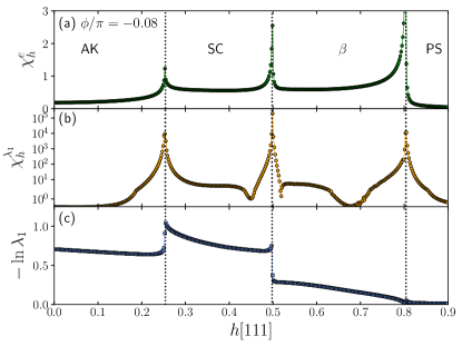
Figure 8: Field sweep of the phase diagram in the AFM Kitaev region at $\phi=-0.08\pi$. (a) $\chi_{h}^{e}$ versus $h[111]$. (b) $\chi_{h}^{\lambda_{1}}$ versus $h[111]$, note the logarithmic scale. (c) Lowest edge of entanglement spectrum, $-\ln\lambda_{1}$ from $\rho_{L/2-1}$ versus $h[111]$. All results in (a), (b) and (c) are from high precision iDMRG calculations with a unit cell of 60. The dashed vertical lines correspond to transitions at field values of $h[111]$ of $0.254$(AK-SC), $0.498$ (SC-$\beta$) and $0.804$ ($\beta$-PS).

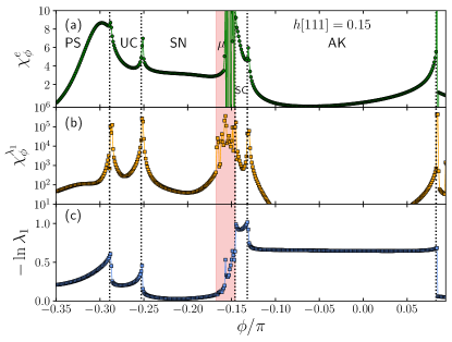
Figure 9: Angle sweep of the phase diagram in the AFM Kitaev region at $h=0.15$. (a) $\chi_{\phi}^{e}$ versus $\phi/\pi$, note the almost imperceptible divergence in $\chi_{\phi}^{e}$ at $\phi=-0.289\pi$. (b) $\chi_{\phi}^{\lambda_{1}}$ versus $\phi/\pi$, note the logarithmic scale. (c) Lowest edge of entanglement spectrum, $-\ln\lambda_{1}$ from $\rho_{L/2-1}$ versus $\phi/\pi$. All results in (a), (b) and (c) are from high precision iDMRG calculations with a unit cell of 60. The dashed vertical lines correspond to transitions at angles $\phi/\pi$ of $-0.289$(PS-UC), $-0.253$ (UC-SN), $-0.146$ ($\mu$-SC), $-0.132$ (SC-AK) and $0.083$ (AK-FM${}_{U_{6}}$). The light red coloring denotes a region of $\phi/\pi$ where convergence of the iDMRG is problematic.

V.1.4 Field and angle sweeps

To further investigate the sharpness of the phase transitions occurring in Fig. 4 we have performed high precision sweeps at constant $\phi=-0.08\pi$ and constant $h[111]=0.15$. The positions of these sweeps are shown as the dotted lines in Fig. 4(b). Our results are shown in Fig. 8 for constant $\phi=-0.08\pi$ and in Fig. 9 for constant $h[111]=0.15$. In both case from high precision iDMRG calculations with a unit cell of 60 and a maximal bond dimension of 1,000.

Results for a field sweep from $h[111]=0$ to $0.9$ are shown in Fig. 8 for a constant $\phi=-0.08\pi$. In panels (a), (b) and (c) we show results for $\chi_{h}^{e}$, $\chi_{h}^{\lambda_{1}}$ and $-\ln\lambda_{1}$, respectively. The 3 transitions, AK-SC ($h[111]$=0.254), SC-$\beta$ ($h[111]=0.498$) and $\beta$-PS ($h[111]=0.804$) are very well defined and are in complete agreement between the three different measures. While the $\beta$-PS is not all that visible in $-\ln\lambda_{1}$ it is very clear in $\chi_{h}^{\lambda_{1}}$. Five orders of magnitude variation is observed in $\chi_{h}^{\lambda_{1}}$.

Results for a $\phi$ sweep from $\phi=-0.35\pi$ to $\phi=0.1\pi$ at constant $h[111]=0.15$ are shown in Fig. 9. In panels (a), (b) and (c) we show results for $\chi_{h}^{e}$, $\chi_{h}^{\lambda_{1}}$ and $-\ln\lambda_{1}$, respectively. Five transitions are clearly visible. While the PS-UC transition at $\phi=-0.289\pi$ is easy to miss in $\chi_{h}^{e}$ it is very well defined in $\chi_{h}^{\lambda_{1}}$ and $-\ln\lambda_{1}$. However, there is a precursor peak in $\chi_{h}^{e}$ not associate with a transition (see also Appendix A). The transition SC-AK is clearly defined at $\phi=-0.132\pi$ as the $\mu$ phase is approached from the SC side it is also clear that $\chi_{h}^{e}$, $\chi_{h}^{\lambda_{1}}$ diverge at the $\mu$-SC transition at $\phi=-0.146\pi$. This transition is therefore well defined. On the other hand, the iDMRG fail to achieve good convergence in the light red colored region so the transition from SN to $\mu$ is not clear. As discussed above it is possible that the $\mu$ phase only marks the onset of short range incommensurate correlations in the SN phase and it is not a distinct phase. It is also possible that improved convergence of the iDMRG would show a divergence in $\chi_{h}^{e}$ and $\chi_{h}^{\lambda_{1}}$ inside the lightly red colored region.

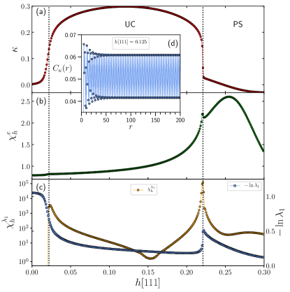
Figure 10: Ordering in the UC-phase. (a) The scalar chirality $\kappa$ versus $h[111]$. (b) $\chi_{h}^{e}$ versus $h[111]$. (c) $\chi_{h}^{\lambda_{1}}$ (orange circles) and $-\ln\lambda_{1}$ (blue circles) versus $h[111]$. (d) The chiral correlation function, $C(r)$ along the ladder at $h[111]=0.125$. All results in (a - d) are from high precision iDMRG calculations with a unit cell of 60 performed at $\phi=-0.27\pi$. The dotted vertical lines denote the transitions at critical fields $h_{1}^{c}=0.022$ and $h^{c}_{2}=0.221$. Note that, the divergence in $\chi_{h}^{e}$ at $h_{1}^{c}$ is imperceptible and very small at $h^{c}_{2}$ where it occurs away from the maximum. However, $\chi_{\phi}^{\lambda_{1}}$ show very well defined peaks at both $h_{1}^{c}$ and $h^{c}_{2}$.

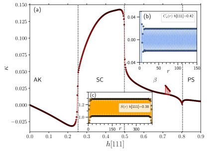
Figure 11: Ordering along $\phi=-0.08\pi$ (AK-, SC- and $\beta$-phase). (a) The scalar chirality $\kappa$ versus $h[111]$. (b) The chiral correlation function, $C(r)$ along the ladder at $h[111]=0.42$. (c) Bipartite entanglement entropy, $S(r)$ versus $r$ at $h[111]=0.38$. Results in (a), (b) are from high precision iDMRG calculations with a unit cell of 60 performed at $\phi=-0.08\pi$ while (c) is from finite-size DMRG with OBC at $\phi=-0.08\pi$, $h[111]=0.38$. The dotted vertical lines denote the transitions at critical fields $h_{1}^{c}=0.254$, $h^{c}_{2}=0.498$ and $h^{c}_{3}=0.804$.

V.2 Scalar Chirality in the UC and SC phases

The presence of a non-zero $\Gamma$ term or the magnetic field raises the possibility of chiral ordering. The chirality without magnetic ordering is rare, unless there are three or four-spin interactions. In 1D system, it was shown that a four-spin interaction produces a long-range scalar chirality.Läuchli et al. (2003) To check the presence of chiral ordering, we label the $i$’th spin on two-legs of the ladder as ${\bf S}_{i,1}$ and ${\bf S}_{i,2}$ where $1$ and $2$ refer to the bottom-leg and top-leg, respectively. We then define the scalar chiral order parameter with ${\bf S}={\bf\sigma}/2$ as follows.

$$\kappa=\langle{\bf\sigma}_{i,1}\cdot\left({\bf\sigma}_{i,2}\times{\bf\sigma}_{i+1,1}\right)\rangle.$$ (11)

This clockwise definition is kept for all triangles made of three spins, for example $\kappa=\langle{\bf\sigma}_{i,2}\cdot\left({\bf\sigma}_{i+1,2}\times{\bf\sigma}_{i+1,1}\right)\rangle$ for upper triangles. If the $\kappa$ is positive (negative), we assign blue (red) arrows $i\to j\to k$ for $\kappa=\langle{\bf\sigma}_{i}\cdot\left({\bf\sigma}_{j}\times{\bf\sigma}_{k}\right)\rangle$ and all even permutations of $i,j,k$, which leads to the clockwise (anti-clockwise) circulation.

It is also of interest to define the scalar chiral correlation function,

$$C_{\kappa}(r)=\langle\kappa_{i}\kappa_{i+r}\rangle,$$ (12)

such that $C_{\kappa}(r)\to\kappa^{2}$. The scalar chiral order parameter breaks spatial symmetries and time reversal symmetry, but not SU(2).

In Fig. 10(a) we show $\kappa$ along a field sweep at constant $\phi=-0.27\pi$ through the UC phase. Results are from high precision iDMRG with a unit cell of 60 sites and a maximal bond dimension of 1,000. In this case we determine $\kappa$ from $C_{\kappa}(r)$ shown in the inset Fig. 10(d) at $h[111]=0.125$. $C_{\kappa}(r)$ reaches a constant value relatively quickly and $\kappa$ is clearly non-zero throughout the phase, reaching significant values at the center of the UC phase. The scalar chirality, $\kappa$

Figure 12: Scalar chirality in the UC-phase. At $h=0.125$ and $\phi=-0.27$, $\kappa=-0.204,-0.298,-0.298,-0.204$ for first four triangles respectively, and then repeat.

is negative throughout the chain and a sketch of the spatial modulation is shown in Fig. 12. Note the edge states appearing on the two opposing legs. Here weaker lines indicate a weaker $\kappa$. Since the $h[111]$ field favors alignment of the spins, which would result in $\kappa=0$, it is rather surprising to observe such a well defined scalar chirality at finite fields. In Fig. 10(b), (c) are shown $\chi_{h}^{e}$ and $\chi_{h}^{\lambda_{1}}$, respectively. While the transitions delimiting the UC phase are almost absent in $\chi_{h}^{e}$, and clearly do not coincide with the broad maximum of $\chi_{h}^{e}$ around $h[11]\sim 0.25$, they are very well defined in $\chi_{h}^{\lambda_{1}}$ and in both cases they coincide with the results for $\kappa$ in Fig. 10(a). As far as we can tell the UC phase does not intersect the zero field axis, instead, as can be seen in Fig. 4 the UC and SN phases meet at a triple point close to $\phi=-0.265\pi$. Entanglement close to this triple point is therefore very elevated which is why $-\ln\lambda_{1}$ (blue squares in Fig. 10(c)) is so high close to zero field.

In Fig. 11 we show iDMRG calculations for $\kappa$ versus $h[111]$ at a fixed $\phi=-0.08$, crossing the AK, SC and $\beta$ phases. $\chi_{h}^{e}$ and $\chi_{h}^{\lambda_{1}}$ along the same line in the phase diagram are shown in Fig. 8. As before, $\kappa$ is obtained from calculations of $C_{\kappa}(r)$ in the large $r$ limit and the sign of $\kappa$ from local direct estimates of $\kappa$. In this case there is a spatial +- alternation of $\kappa$ as shown in Fig. 13 but the magnitude of $\kappa$ is the same for each triangle leading to the zero flux in the system.

Figure 13: Scalar chirality in the SC-phase. At $h=0.42$ and $\phi=-0.08$, $\kappa=0.139,-0.139,-0.139,0.139$ for first four triangles respectively, and then repeat.

Although there is weak chirality in the AK and $\beta$ phases, $\kappa$ is an order of magnitude larger in the SC phase and jumps rather abruptly at the critical points indicated by the dotted lines in Fig. 11. In the inset panel (b) is shown $C_{\kappa}(r)$ versus $r$ at $h[111]=0.42$ which attain a constant value for modest values of $r\sim 20$. Panel (c) in Fig. 11 show the bipartite entanglement obtained from a bi-partition of the system at site $r$. The resulting entanglement entropy $S(r)=-\rm{Tr}\rho_{r}\ln\rho_{r}$ is shown versus $r$ for a finite ladder with $N=400$ and OBC. Clearly, $S(r)$ is close to constant in the middle of the ladder which would be consistent with the existence of a non-zero gap in the SC phase. (See also Appendix C).

Figure 14: Scalar chirality in the AK-phase. At $h=0.2$ and $\phi=-0.08$, $\kappa=-0.0191,0.0191,-0.0466,0.0466$ for first four triangles respectively, and then repeat.

To make a comparison to the AK phase, we also compute the chirality in the AK phase, and its pattern is shown in Fig. 14. $\kappa$ has distinctly different circulations. It has a staggering circulation between upper and lower triangles, but different staggering from the SC phase. For both the AK and SC phases, the magnitude of $\kappa$ is the same for all pairs of triangles, implying that there is zero net-flux in the system. The phase transition from the AK to SC phases is accompanied by the sharp change of both magnitude and distinct pattern of $\kappa$.

V.3 String Order and Mapping to KQ Model

In Ref. Catuneanu et al. (2019) a non-local unitary transformation, $V$, was introduced of the following form: We then define the following unitary (disentangling) operator for an $N$-site chain with OBC:

$$V=\prod_{\begin{subarray}{c}j+1<k\\ j\ \mathrm{odd},\ k\ \mathrm{odd}\\ j=1,\ldots N-3\\ k=3,\ldots N-1\end{subarray}}U(j,k).$$ (13)

With the individual $U(j,k)$ given as follows:

$$U(j,k)=e^{i\pi(S^{y}_{j}+S^{y}_{j+1})\cdot(S^{x}_{k}+S^{x}_{k+1})}.$$ (14)

At the AFM Kitaev point, $\phi=0$, $V$ maps the ladder with open boundary conditions to a so called dangling-Z model, $H_{d-Z}$, that has long-range ordering in $\langle\tilde{S}^{z}_{i}\tilde{S}^{z}_{i+r}\rangle$, where $\tilde{S}$ are the spins in $H_{d-Z}$ Catuneanu et al. (2019). If this correlation function is transformed back to the original Kitaev ladder one arrives at a string correlation function of the following form:

$$\langle{\cal O}^{z}(r)\rangle = 4\langle\tilde{S}_{2}^{z}\tilde{S}_{2+r}^{z}\rangle=(-1)^{\left\lfloor{(r+1)/2}\right\rfloor}$$ (18)

$$\times \left\{\begin{array}[]{rl}\langle\sigma_{1}^{y}\sigma_{2}^{x}\left(\prod_{k=3}^{r}\sigma_{k}^{z}\right)\sigma_{r+1}^{x}\sigma_{r+2}^{y}\rangle&\mbox{ $r$ even}\\ \\ \langle\sigma_{1}^{y}\sigma_{2}^{x}\left(\prod_{k=3}^{r+1}\sigma_{k}^{z}\right)\sigma_{r+2}^{y}\sigma_{r+3}^{x}\rangle&\mbox{ $r$ odd}\end{array}\right.$$

Note that, in Ref. Catuneanu et al. (2019) some of the indices in Eq. (18) in the expression for $r$ even were incorrect. With this definition we find that the usual plaquette operator Kitaev (2006) $W_{p}\equiv{\cal O}^{z}(r=4)$. $W_{p}$ is often used to characterize the AK phase. See Appendix D.

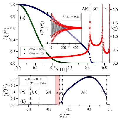
Figure 15: String order $\langle{\cal O}^{z}\rangle$ versus field in the AFM Kitaev region. (a) $\langle{\cal O}^{z}(r=100)\rangle$ (blue triangles) and $\langle{\cal O}^{z}(r=100)\rangle$ (green circles) versus $h[111]$ at the AFM Kitaev point $\phi=0$ shown along with $\chi_{h}^{e}$. Open red circles show $\chi_{h}^{e}$. The inset shows $\langle O^{z}(r)\rangle$ (red cirles) versus $r$ at $h[111]=0.25$, $\phi=0$. (b) $\langle{\cal O}^{z}(r=100)\rangle$ (blue triangles) versus $\phi/\pi$ at fixed $h[111]=0.15$. Results in (a), (b) are from high precision iDMRG calculations with a unit cell of 60. The dotted vertical lines denote the transitions at critical fields determined from divergences in $\chi_{h}^{e}$ and $\chi_{h}^{\lambda_{1}}$.

Results for ${\cal O}^{z}$ are shown in Fig. 15. In the presence of a non-zero magnetic field or a non-zero $\Gamma$ the string order correlation function ${\cal O}^{z}(r)$ is not long-range. Instead, as shown in the inset in Fig. 15(a) for $h[111]=0.25$, it decays exponentially to zero. However, the length scale describing this exponential decay is extremely large, often exceeding hundreds or for small enough $\Gamma$, $h[111]$, thousands of lattice spacings. The extent of the AK phase can therefore be determined by determining ${\cal O}^{z}(r=100)$ or ${\cal O}^{z}(r=900)$ which remain non-zero through out the AK phase. This is illustrated in Fig. 15(a) where both ${\cal O}^{z}(r=100)$ (solid blue triangles) and ${\cal O}^{z}(r=900)$ (solid green circles) are plotted versus $h[111]$ along side $\chi_{h}^{e}$ (open red circles) at $\phi=0$. Clearly, ${\cal O}^{z}(r=100)$ drops abruptly towards zero at the phase transition between AK and the SC phase. Fig. 15(b) shows ${\cal O}^{z}(r=100)$ versus $\phi$ at fixed $h[111]=0.15$ again abrupt changes in ${\cal O}^{z}(r=100)$ are observed at the boundary of the AK phase.

V.3.1 Mapping to KQ model

It is of considerable interest to explore non-local unitary operators that will lead to string order correlation functions showing long-range order also for $\Gamma\neq 0$. We begin by considering how the ladder is transformed under the $U_{6}$ transformation previously described. If the spins on one leg of the ladder are numbered $i=1\ldots N/2$ we assign them a second label $k=(i-1)\mathrm{mod}6+1$ on the second leg we assign the label $k=(i+2)\mathrm{mod}6+1$. With this labelling we introduce the following notation for the transformed bonds

$$x^{\prime}\ :\ -KS^{x}_{i}S^{x}_{j}-\Gamma(S^{y}_{i}S^{y}_{j}+S^{z}_{i}S^{z}_{j})$$

$$y^{\prime}\ :\ -KS^{y}_{i}S^{y}_{j}-\Gamma(S^{x}_{i}S^{x}_{j}+S^{z}_{i}S^{z}_{j})$$

$$z^{\prime}\ :\ -KS^{z}_{i}S^{z}_{j}-\Gamma(S^{x}_{i}S^{x}_{j}+S^{y}_{i}S^{y}_{j})$$ (19)

Here $j$ is a nearest neighbor site. With this notation we can represent the transformed ladder using the following picture, Fig. 16

Figure 16: The KG ladder after the $U_{6}$ local transformation

We then consider the zero field case with OBC and change notation slightly compared to Ref. Catuneanu et al. (2019) by using an equivalent non-local unitary operator:

$$W=\prod_{\begin{subarray}{c}j+1<k\\ j\ \mathrm{odd},\ k\ \mathrm{odd}\\ j=1,\ldots N-3\\ k=3,\ldots N-1\end{subarray}}w(j,k).$$ (20)

With the individual $w(j,k)$ given as follows:

$$w(j,k)=e^{i\pi(S^{y}_{j}+S^{y}_{j+1})\cdot(S^{z}_{k}+S^{z}_{k+1})},$$ (21)

and $W^{\dagger}=W$. With this definition of $W$ we see that on the vertical bonds of the ladder $W$ leaves all interactions unchanged

$$WS_{1}^{\alpha}S_{2}^{\alpha}W=S_{1}^{\alpha}S_{2}^{\alpha},\ \ WS_{3}^{\alpha}S_{4}^{\alpha}W=S_{3}^{\alpha}S_{4}^{\alpha},\ \ldots$$ (22)

However, on horizontal bonds we find

$$WS_{2}^{y}S_{4}^{y}W=-S_{1}^{y}S_{4}^{y},\ \ WS_{3}^{y}S_{5}^{y}W=-S_{4}^{y}S_{5}^{y},\ \ldots$$ (23)

Note that $W$ effectively moves the bond and changes the sign of the interaction. Likewise, we get for the horizontal $zz$ bonds

$$VS_{2}^{z}S_{4}^{z}V=-S_{2}^{z}S_{3}^{z},\ \ VS_{3}^{z}S_{5}^{z}V=-S_{3}^{z}S_{6}^{z},\ \ldots$$ (24)

However, the horizontal $xx$ bonds give rise to non-trivial 4-spin interactions. Specifically:

$$VS_{2}^{x}S_{4}^{x}V=-\sigma_{1}^{y}S_{2}^{z}\sigma_{3}^{z}S_{4}^{y},\ \ VS_{3}^{x}S_{5}^{x}V=-S_{3}^{z}\sigma_{4}^{y}S_{5}^{y}\sigma_{6}^{z},\ldots$$ (25)

thereby coupling the four spins around a plaquette. We then introduce additional notation for transformed bonds

$$K_{z}\Gamma_{y}\ :\ KS^{z}_{i}S^{z}_{j}+\Gamma S^{y}_{i}S^{y}_{j}$$

$$K_{y}\Gamma_{z}\ :\ KS^{y}_{i}S^{y}_{j}+\Gamma S^{z}_{i}S^{z}_{j}$$

$$\Gamma_{y}\Gamma_{z}\ :\ \Gamma S^{y}_{i}S^{y}_{j}+\Gamma S^{z}_{i}S^{z}_{j}$$

$$\Gamma^{k,l}_{i,j}\ :\ 4\Gamma(S^{z}_{k}S^{z}_{l}S^{y}_{i}S^{y}_{j}+S^{y}_{k}S^{y}_{l}S^{z}_{i}S^{z}_{j})$$

$$K^{k,l}_{i,j}\ :\ 4K(S^{z}_{k}S^{z}_{l}S^{y}_{i}S^{y}_{j}+S^{y}_{k}S^{y}_{l}S^{z}_{i}S^{z}_{j})$$ (26)

With this notation in hand we can now apply the $W$ transformation to the $U_{6}$ transformed ladder shown in Fig. 16. The resulting Hamiltonian can be drawn in the manner shown in Fig. 17.

Figure 17: $H_{KQ}$: The KG ladder after the $U_{6}$ transformation followed by the $W$ transformation

It is quite remarkable that the $W$ transformation has generated four-spin exchange terms. We call this $H_{KQ}$ Hamiltonian the KQ ladder since the model is a close cousin of JQ models Sandvik (2007) extensively studied as models of deconfined criticality Senthil et al. (2004). Unexpectedly, the ground-state for the KQ model in the AK phase has a significant overlap with a rung-triplet state. If we define:

$$t_{x}=(|\uparrow\uparrow\rangle-|\downarrow\downarrow\rangle)/\sqrt{2}$$

$$t_{y}=(|\uparrow\uparrow\rangle+|\downarrow\downarrow\rangle)/\sqrt{2}$$

$$t_{z}=(|\uparrow\downarrow\rangle+|\downarrow\uparrow\rangle)/\sqrt{2}$$ (27)

Then we can pictorially draw the rung-triplet state as shown in Fig. 18.

Figure 18: The rung-triplet states A and B for the KQ model

With OBC there is another energetically equivalent rung-triplet state obtained by translation as shown in Fig. 18. The two states approximates the doublet ground-state of the KQ model. Surprisingly, the unit cell for these triplet states are 12 sites and not as one might have expected from the structure of $H_{KG}$, 6 sites. Ordering of this type has previously been studied using SOP’s inspired by the studies of $s=1$ spin chains. If $\tau_{i}^{\alpha}=S^{\alpha}_{i,1}+S^{\alpha}_{i+1,2}$ are the sum of two diagonally situated spins, one defines Kim et al. (2000); Fáth et al. (2001):

$${\cal O}_{\mathrm{even}}^{\alpha}(r)=-\langle\tau_{i}^{\alpha}\exp(i\pi\sum_{l=i+1}^{i+r-1}\tau_{l}^{\alpha})\tau_{i+r}^{\alpha}\rangle.$$ (28)

This order parameter has been used to distinguish topologically distinct phases in Heisenberg ladders and is non-zero in the rung-singlet phase where the topological number is even.

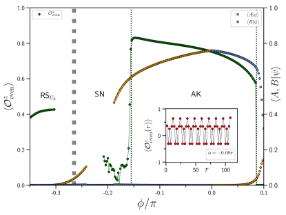
Figure 19: String order parameter $\langle{\cal O}_{\mathrm{even}}^{z}\rangle$ versus field (green circles) in the AFM Kitaev region for $H_{KQ}$ with $N=120$. Results are shown along side the overlaps $\langle A|\psi\rangle$ and $\langle B|\psi\rangle$ from calculations with $N=12$. Results are from high precision DMRG calculations with OBC. The dotted vertical lines denote the transitions at critical fields determined from divergences in $\chi_{h}^{e}$ and $\chi_{h}^{\lambda_{1}}$.

In Fig. 19 we show results for ${\cal O}_{\mathrm{even}}^{z}$ estimated from ${\cal O}_{\mathrm{even}}^{z}(r)$ in the large $r$ limit on systems with $N=120$ and OBC. This SOP drops abruptly to zero at the limits of the AK phase and, as can be seen from the inset, there is no exponential decay observed in ${\cal O}_{\mathrm{even}}^{z}(r)$ which instead quickly attains a constant value. As expected, ${\cal O}_{\mathrm{even}}^{z}$ is also non-zero in the RS${}_{U_{6}}$ phase, but clearly zero in the SN phase. Also shown in Fig. 19 are the overlaps with the rung-triplet states $\langle A|\psi\rangle$ and $\langle B|\psi\rangle$ as obtained from small $N=12$ systems with OBC. There are significant finite-size effects at the boundaries of the AK phase for the overlaps, although they drop to zero outside the AK phase the critical points are not as well defined as for ${\cal O}_{\mathrm{even}}^{z}$. The rung-triplet states shown in Fig. 19 are approximate and for $N>12$ different linear combinations enter such that with the simple definitions of the rung-triplet states above $\langle A|\psi\rangle$ and $\langle B|\psi\rangle$ tend to zero as $N\to\infty$. However, ${\cal O}_{\mathrm{even}}^{z}$ is clearly non-zero in the AK phase and in the KQ model this phase is therefore topologically equivalent to the Haldane like phases observed in Heisenberg ladders with even topological number. Since the KQ model is related to the KG model through unitary transformations the same must be true for the KG ladder throughout the AK phase. Calculations in the FK phase show that ${\cal O}_{\mathrm{even}}^{z}$ is also clearly non-zero in zero field throughout that phase but drops to zero in the A$\Gamma$ phase.

VI Comparison: the honeycomb KG model

It is important to note that the pure AFM Kitaev under the magnetic field studied by DMRG and 24-site ED exhibits an intermediate gapless phase before it polarizes. A U(1) spin liquid was suggested for this field-induced gapless phase Hickey and Trebst (2019). However, in the two-leg ladder, we found five distinct phases including AK  SC, $\gamma$, $\eta$, and PS at the pure AFM Kitaev point (white thin line at $\phi=0$ in Fig. 4), as the magnetic field increases. There are several factors including the obvious geometry difference that may result in the different results between the 24-site honeycomb cluster and current results. To understand possible origins of the difference, we investigate the following systems at AFM Kitaev point, $\phi=0$.

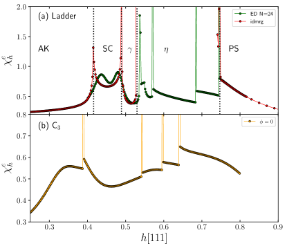
Figure 20: Comparison between the two leg ladder and the 24-site C₃ symmetric honeycomb geometry at $\phi=0$. (a) The ladder: $\chi_{h}^{e}$ versus $h[111]$ as obtained from ED with N=24 (green circles) and from high precision idmrg with a unit cell of 60 (red circles). (b) The C₃ symmetric honeycomb geometry: $\chi_{h}^{e}$ versus $h[111]$ as obtained from ED with N=24 (orange circles). The critical fields are at $0.388$, $0.543$, $0.598$ and $0.641$.

First we study the 24-site ladder using ED and compare the result with iDMRG with a unit cell of 60, to understand the finite size effects. The results of $\chi_{h}^{e}$ are shown in Fig. 19 (a) where the red and green dots are obtained by iDMRG and ED, respectively. Note that, due to problems with convergence there are no iDMRG results in the $\eta$ phase. The sharp transitions seen in the iDMRG between AK and SC at $h[111]=0.416$, and between SC and $\gamma$ at $h[111]=0.489$ are replaced by broad bumps in ED, while the transition between $\gamma$ and $\eta$ at $h[111]=0.530$ in the iDMRG is also sharp in the ED results. The transition to the PS phase occurs around the same field strength for both ED and iDMRG, $h[111]=0.747$. There are a couple of sharp features within $\eta$ phase only found in ED, which we assign to finite size effects. Other than these additional peaks in $\eta$ phase, the results are remarkably similar.

We also investigate the 24-site C₃ symmetric honeycomb cluster using the ED. $\chi_{h}^{e}$ is shown in Fig. 19 (b), where $h$ sweeps from 0 to 0.8 by $\delta h=0.001$, much smaller steps than previous studies.Hickey and Trebst (2019) There are four transitions found at $h[111]=0.388$, $0.543$, $0.598$ and $0.641$, which may suggest three intermediate phases. For comparison Ref. Hickey and Trebst (2019) only find 2 transitions performing ED on the same 24-site C₃ cluster, presumably due to a larger $\delta h$. However, based on the finite size effects found in 24-site ladder ED, we suspect that there are significant finite size effects in this system that makes it hard to determine whether these phases correspond to the SC, $\gamma$ and $\eta$ phases, or only one (SC) or two phases survive in the thermodynamic limit. Indeed when the field is tilted away from the c-axis, there are only two transitions found in the 24-site C₃ clusterHickey and Trebst (2019), while the three intermediate phases – SC, $\gamma$ and $\eta$ – found in the iDMRG ladder persist even in the titlted field (see Appendix E). Given that $\gamma$ and $\eta$ are incommensurate magnetic phases, and thus sensitive to the shape of cluster, we speculate that they likely turn into another type of incommensurate phase confined in the C₃ symmetric cluster. The chirality of the SC phase may survive in the honeycomb cluster defined at a triangle made of nearest neighbors or next nearest neighbors of honeycomb lattice. This is an excellent topic for future study, as it requires a bigger size system to check the chiral correlation $C(r)$.

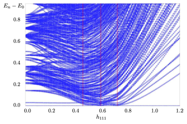
Figure 21: The energy spectrum of the pure AFM Kitaev limit under the [111] field using 2$\times$ 6 ladder.

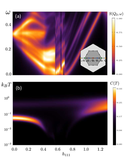
Figure 22: (a) Dynamical spin structure factor $S(Q_{2},\omega)$ at the wave-vector of Q₂ defined in the BZ figure shown in the inset and (b) specific heat $C(T)$ of the pure AFM Kitaev limit under the $[111]$ field using 2$\times$ 6 ladder.

To shed further light on the occurrence of gapless excitations in 24-site C₃ cluster in ED, we choose an even smaller cluster of 2 $\times$ 6 ladder, and compute various quantities under the [111] field. The energy spectrum is shown in Fig. 21 which indicates three phase transitions (red dashed lines obtained from $\chi_{h}^{e}$ with four phases; the low-field Kitaev phase changes to a field-induced intermediate phases, which then transitions to another intermediate phase, before it becomes the polarized state. The collapse of the excitations is remarkably similar to 24-site C₃ cluster, suggesting that the intermediate gapless excitation feature is insensitive to the cluster size and shape, even though the critical fields where such phases arise change depending on the shape. The qualitative behaviour is similar to the 24-site ladder and C₃ ED presented above. However, it is not clear if there is one or two intermediate phases, as the incommensurability of $\gamma$ and $\eta$ phases would suffer from the change of cluster size and shape, as discussed above. The dynamical structure factor at a particular momentum $Q_{2}$ (shown in the inset) and the specific heat in the field are shown in Fig. 22 (a) and (b), respectively. The first intermediate phase is likely disordered, while the second intermediate phase likely exhibits incommensurate ordering. They do not exhibit well-defined excitation spectra in the specific heat similar to what is observed in the C₃ 24-site ED.Hickey and Trebst (2019) While it is a 12-sites ladder geometry, the qualitative results are incredibly similar to the DMRG phase diagram at the $\phi=0$ AFM Kitaev point under the field and the 24-site C₃ symmetric honeycomb geometry results.Hickey and Trebst (2019) It shows a dense energy spectrum in the intermediate states of both disordered (SC) and field-induced incommensurate ($\eta$ or $\gamma$) phase.

The above analysis with small ladder and C₃ cluster suggests that the AFM Kitaev 2D honeycomb model under the field may also display a richer phase diagram than what has been reported, and a high resolution numerical calculation is required to refine the phase diagram. Since the $\gamma$ or $\eta$ phases also show a dense energy spectrum, it is important to differentiate the U(1) spin liquid from the incommensurate phases in the honeycomb AFM Kitaev limit. Comparing the critical field above which gapless spin liquid occurs in 24-site EDHickey and Trebst (2019), it is likely that the disordered SC phase with enhanced entanglement and edge excitations extends to the gapless spin liquid in the honeycomb lattice, and the incommensurate phase is mixed with a polarized state, which was missed in 24-site ED of the honeycomb lattice. We conclude that the ladder model at the AFM Kitaev limit captures both disordered and incommensurate magnetically ordered phases under the magnetic field, and offers future directions in searching for a spin liquid in the honeycomb KG model.

VII summary and discussion

The KG model consists of two bond-dependent interactions, namely the Kitaev and Gamma interactions. The Kitaev interaction on the honeycomb lattice exhibits a spin liquid with fractionalized excitations. In particular, under a time-reversal symmetry breaking term, the excitations obey non-Abelian statistics. The Gamma interaction is another highly frustrated interaction leading to a macroscopic degeneracy in the classical limit, and quantum fluctuations do not lift the degeneracy found in the AFM classical Gamma model.Rousochatzakis and Perkins (2017)

Since these two frustrating interactions are dominant interactions in realistic descriptions of emerging Kitaev candidates such as RuCl₃, the minimal KG model was initially proposed to understand RuCl₃.Catuneanu et al. (2018); Gordon et al. (2019) The magnetic field has been a crucial parameter, as the system may undergo a transition into a field-induced disordered phase before the trivial PS appears. Aside from its relevance to Kitaev materials, the minimal KG model may offer a playground to discover exotic spin liquids due to the combined frustration of the K and Gamma term, and thus has been extensively studied for the last few years. Given the huge phase space of AFM and FM Kitaev, AFM and FM Gamma, and the field, most studies are limited to a narrow phase space focusing on the FM Kitaev and AFM Kitaev regions. Many numerical methods have been used to identify phases of the extended Kitaev model under the field and intriguing results were reported near AFM Kitaev and FM Kitaev regions including the field-induced gapless U(1) spin liquid near the AFM Kitaev region.Hickey and Trebst (2019) However, it is not clear if the gapless excitations are due to more conventional physics such as incommensurate ordering.

Here we investigate the entire phase space of the KG ladder model under the magnetic field. While the geometry is limited to the ladder, it has the great advantage of allowing for high numerical precision such as accessing iDMRG with a high precision mode with a unit cell of 60 and a maximal bond dimension of 1000. Numerical calculations are therefore very well controlled. We found an extremely rich phase diagram of the KG model under the field. Among fifteen distinct phases identified, nine phases appear near the AFM Kitaev region alone. In the zero field, there is a quadrupole ordered phase named SN, two magnetically ordered phases (FM${}_{U_{6}}$ and RS${}_{U_{6}}$) straightforward to understand from the mapping of 6-site transformation, and the disordered AK phase. It is interesting that the SN phase found in the KG chainYang et al. (2020b) survives in the ladder. Other than the AK phase (which becomes the Kitaev spin liquid in the 2D limit), the zero-field phases are ordered and the entanglement entropy is rather low. Under the field, highly entangled phases emerge. Apart from several incommensurate magnetic ordered phases, two highly entangled phases denoted by SC referring staggered chirality and UC uniform chirality are induced by the field. These phases exhibit distinct chirality orderings and high entanglement entropy with gapless edge excitations when the boundary is open.

The ladder results presented here offer several important insights in possible spin liquids and not-yet-identified phases in the 2D honeycomb lattice. We would like to recall that the pure Kitaev model in the ladder corresponding to AK and FK in this study is gapped, where the ladder can be viewed as a coupled chains.Feng et al. (2007b) As the number of chains grows, the ground state changes between gapped and gapless depending on the even and odd numbers of the chains, and eventually maps to the 2D Kitaev spin liquid in a true 2D limit. The AK and FK are gapped due to the geometry of the ladder, but its nature, magnetically disordered with high entanglement, is captured in the ladder model. Applying similar logic, we suggest that the disordered SC phase is related to the spin liquid in the 2D limit. The SC phase has a staggered chirality but different patterns from the AK phase in field, which differentiate the two phases. While it is gapped in the ladder, it may become gapless as the number of chains grows.

Interestingly the previous DMRG studies on the pure AFM Kitaev point ($\phi=0$) under the $[111]$-field with three to five number of legs reported different central charge in the intermediate phase. For three-leg chains, the central charge $c=1$Jiang et al. (2018) was reported, while for four- and five-leg chains, $c=0$Jiang et al. (2018) and $c\sim 4$Gohlke et al. (2018) respectively were found. Based on the central charge arguments, these studies indicate that there are gapless excitations associated with a spinon Fermi surface in the intermediate field region. It was suggested that the spinon Fermi surface pockets are around $K/K^{\prime}$- and $\Gamma$-point of the first Brillouin zoneJiang et al. (2018), while the other DMRG study proposed the pockets around $M$- and $\Gamma$-points.Patel and Trivedi (2019). The existence of a spinon Fermi surface in momentum space is yet to be determined.

While the most previous studies reported the field-induced intermediate phase as a single phase at the pure AFM Kitaev $\phi=0$ point in the $[111]$-field Zhu et al. (2018); Hickey and Trebst (2019); Jiang et al. (2018); Ronquillo et al. (2019); Patel and Trivedi (2019); Nasu et al. (2018), a separation of the intermediate region into three phases was noted in Gohlke et al. (2018), and the middle phase, which corresponds to the $\gamma$ phase in the ladder, grows in extent with larger bond dimensions where five-legs were used. We find three different intermediate phases, SC, $\gamma$ and $\eta$ in the ladder at $\phi=0$. While the $\gamma$ phase occupies a tiny phase space in the ladder, it is possible that this gapless incommensurate $\gamma$ extends its phase space, as the number of chain grows. This implies that the chiral spin liquid candidate SC may require a finite FM $\Gamma$ interaction, as it generates more frustration. The SC phase with long-range chirality and enhanced entanglement appearing at the intermediate field region of the ladder likely evolves to a field-induced spin liquid with a finite staggered chirality.

The UC phase is another candidate of spin liquid. It has uniform chirality pattern with high entanglement with a finite net flux, and it appears at very low field between SN and 6-site transformed FM phase. This phase space has not been well explored in honeycomb clusters, and we suggest further studies in this region to look for a possible spin liquid. The nature of the SC and UC phases and statistics of excitations in these phases are excellent topics for future study.

Possible incommensurate orderings in the 2D limit also deserves some discussion. Incommensurate orderings are generally difficult to pin down, as they depend on the size of cluster, and the ordering wave-vector itself changes even inside a phase due to the nature of incommensuration. In the ladder, we found several incommensurate orderings. Some has high entanglement indicating a quantum order coexisting with an incommensurate ordering. The possibility of incommensurate ordering has been excluded in the C₃ symmetric cluster, mainly because of technical difficulty set by a limited size. Our ladder study suggests several incommensurate orderings may be present in the 2D honeycomb lattice, and future studies on such a possibility on larger honeycomb clusters are desirable.

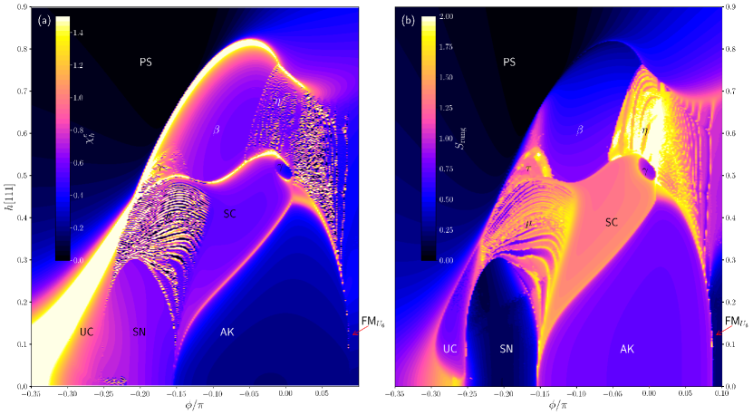
Figure 23: (a) Phase diagram for the AFM Kitaev region of the two-leg ladder KG model under the magnetic field along [111]-axis as obtained from $\chi^{e}_{h}$. Note the absence of a clear definition of the UC phase. (b) Phase diagram for the AFM Kitaev region of the two-leg ladder KG model under the magnetic field along [111]-axis as obtained from $S_{\mathrm{rung}}$, the bipartite entanglement entropy at $N/2-1$. This partition cuts the middle rung of the ladder. Note the clear definition of the UC phase. All results are from high throughput iDMRG calculations with a unit cell of 24 sites, with $\Delta\phi=0.002\pi$, $\Delta h[111]=0.002$

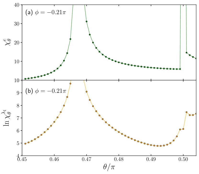
Figure 24: (a) $\chi_{\theta}^{e}$ and (b) $\ln\chi_{\theta}^{\lambda_{1}}$ versus $\theta$ at a fixed $\phi=-0.21\pi$ inside the SN phase where we set $J\equiv K\cos{\theta}$ for the KG ladder. It shows a clear first order transition at $J=0$ indicating a first order transition point. Results are from high precision iDMRG with unit cell of 60.

Appendix A Phase diagram of the AFM region from, $\chi^{e}_{h}$ and $S_{\mathrm{rung}}$

In addition to the phase diagram determined from $-\ln\lambda_{1}$ and $\chi^{\lambda_{1}}_{\phi}$ shown in Fig. 4 of the main text it is useful to also consider $\chi^{e}_{h}=-\partial^{2}e_{0}/\partial h^{2}$, with $e_{0}$ the ground-state energy per spin. This is shown in Fig. 23. All the phases except for the UC phase are clearly visible in Fig. 23(a). As described in the main text, the transition to the UC phase is subtle and easily missed in $\chi^{e}_{h}$. However, the precursor ‘bump’ to this phase transition (see Fig. 9(a) of the main text) is clearly visible in the lower left corner of Fig. 23(a) as the large band of bright yellow, however, this feature is not associated with any real phase transition.

Another useful depiction of the AFM Kitaev region phase diagram can be obtained from $S_{\mathrm{rung}}$. With $\rho_{N/2-1}$ the reduced density matrix of the first $N/2-1$ sites of the ladder, the bipartite entanglement entropy is obtained as $S_{\mathrm{rung}}=-\mathrm{Tr}\rho_{N/2-1}\ln\rho_{N/2-1}$, with the partition cutting the middle rung (and both legs) of the ladder. Our results for this quantity are shown in Fig. 23(b). In this case the UC phase along with all the other phases are clearly defined. Regions of increased values of $S_{\mathrm{rung}}$ are visible as bright yellow colored bands in the $\mu$ and $\tau$ phases. These bands likely describe lock-ins to particular magnetic orderings compatible with the unit cell used in the calculations. The ’heart of entanglement’, with its elevated entanglement, encompassing the $\mu$, SC and $\gamma$ phases is beautifully illuminated in yellow and orange colors. Even higher bipartite entanglement is present in the $\eta$ phase with its bright yellow colors.

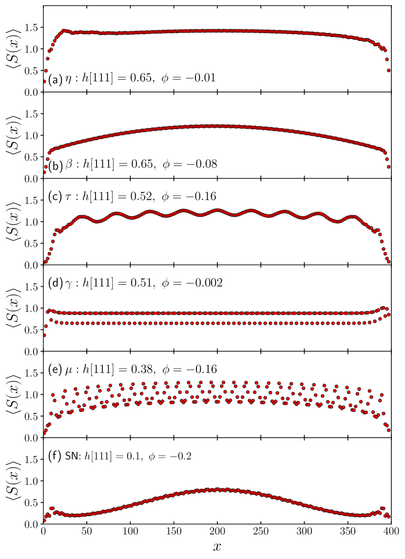
Figure 25: The bi-partite rung entanglement entropy from a cut at site $x$ (odd), $S_{\mathrm{rung}}(x)$ versus $x$ at six different points in the phase diagram indicated in Fig. 4 (main text) representing the (a) $\eta$, (b) $\beta$, (c) $\tau$, (d) $\gamma$, (e) $\mu$ and (f) SN phases. Results are from finite-size DMRG calculations for total system size $N=400$ with open boundary conditions.

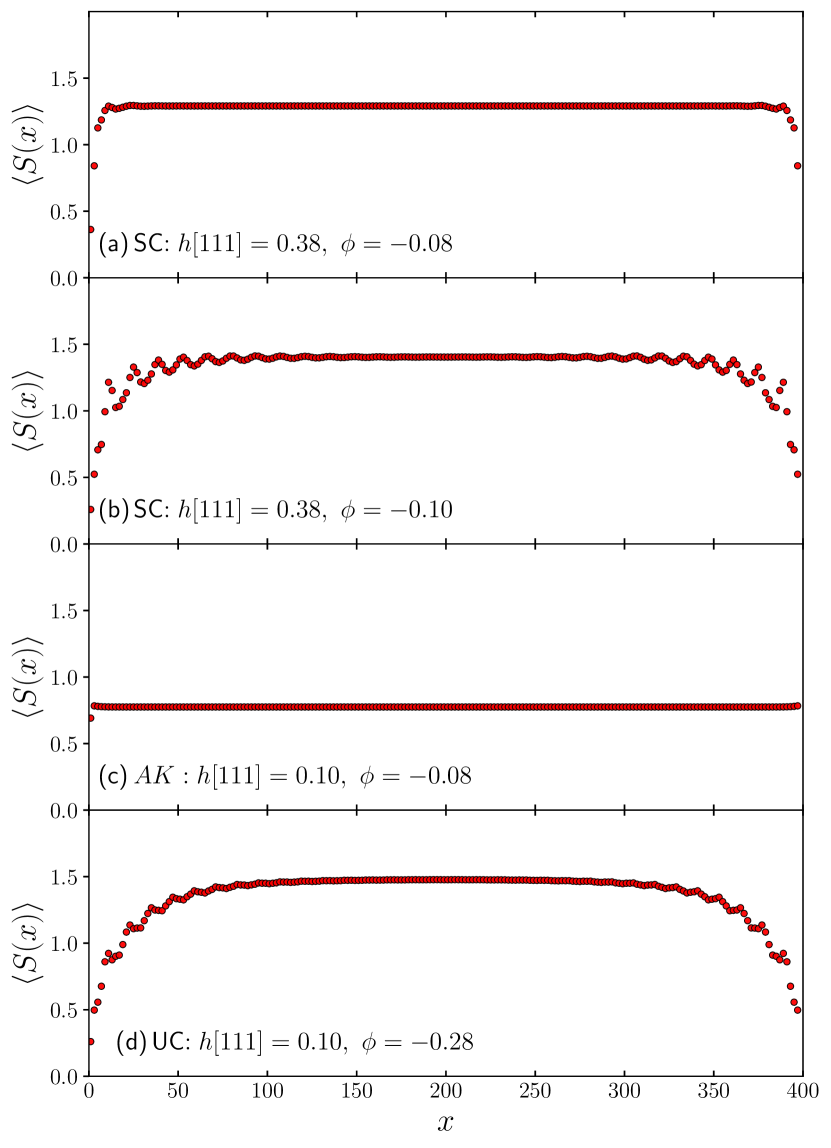
Figure 26: The bi-partite rung entanglement entropy from a cut at site $x$ (odd), $S_{\mathrm{rung}}(x)$ versus $x$ at four different points in the phase diagram indicated in Fig. 4 (main text) representing (a) the SC-phase at $h[111]=0.38$, $\phi=-0.08\pi$, (b) the SC-phase at $h[111]=0.38$, $\phi=-0.10\pi$, (c) the AK-phase and (d) the UC phase. Results are from finite-size DMRG calculations for total system size $N=400$ with open boundary conditions.

Appendix B SN phase at zero field

To understand the zero-field SN phase where the DMRG with OBC finds two different magnetic orderings depending on the system, we introduce an additional Heisenberg coupling, $J=K\cos{\theta}$, and study (a) the energy susceptibility $\chi_{\theta}^{e}$ and (b) $\ln\chi_{\theta}^{\lambda_{1}}$ versus $\theta$ at a fixed $\phi=-0.21\pi$. This is to check if there is a first order transition as a function of $J$ occuring along the line of the SN. Indeed a clear first order transition is found in the energy suscepbility at $\theta=\pi/2$, i.e. $J=0$ as shown in Fig. 24. We conclude that the phase space denoted by the SN is a line of first order transitions separating two different magnetic ordering states. Since the nematic (spin-quadropole) order is finite in both ordered states, we keep the name the SN for this line of first order transitions, throughout the paper.

Appendix C Bipartite entanglement in the AFM Kitaev region

If we instead of defining the reduced density matrix at $x=N/2-1$, as we did when considering $S_{\mathrm{rung}}$, but instead at a general $x$ always taken to be odd, we obtain the bipartite rung entanglement entropy, $S_{\mathrm{rung}}(x)=-\mathrm{Tr}\rho_{x}\ln\rho_{x}$. Our results for $S_{\mathrm{rung}}(x)$ at various points in the AFM Kitaev region are shown in Fig. 25 and 26 corresponding to the same points as the ones shown in Fig. 5, 6 in the main text. It is well established that the entanglement entropy is bounded Hastings (2007); Gottesman and Hastings (2010) in systems with a gap. For a system with a gap $S_{\mathrm{rung}}(x)$ should then attain a plateau in the middle of the chain for long enough ladders when that limit is attained. On the other hand, for a 1D critical gapless system with open boundary conditions we expect Calabrese and Cardy (2004)

$$S(x)=\frac{c}{6}\ln\left[\frac{2N}{\pi}\sin\left(\frac{\pi x}{N}\right)\right]+\ln g+s_{1}/2.$$ (29)

Here $c$ is the central charge, $g$ the universal ground-state degeneracy Affleck and Ludwig (1991) and $S_{1}$ a non-universal constant. As is well known, the entanglement therefore grows logarithmically and is not bounded. The fact that a plateau is observed in the middle of the ladder for $S_{\mathrm{rung}}$ is therefore consistent with a gap.

From the results shown in Fig. 25 and 26 the behavior of $S_{\mathrm{rung}}(x)$ in the SC, AK, UC and $\gamma$ phases are therefore indicative of a gapped phase. The results for the remaining phases are more consistent with a gapless phase, although without giving a clear fit to the form Eq. (29) and it is not possible to extract the central charge.

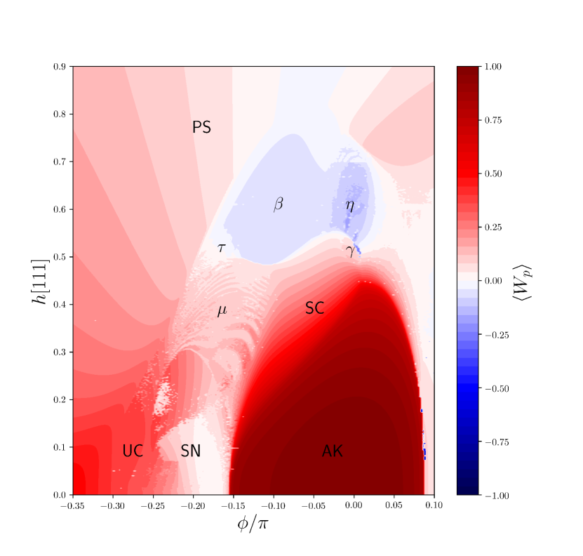
Figure 27: The honeycomb plaquette operator, $W_{p}$, through out the AFM Kitaev region for the two-leg ladder KG model under the magnetic field along [111]-axis. Note the negative values in the $\beta$ and $\eta$ phases. All results are from high throughput iDMRG calculations with a unit cell of 24 sites, with $\Delta\phi=0.002\pi$, $\Delta h[111]=0.002$. The white speckles are missing data points.

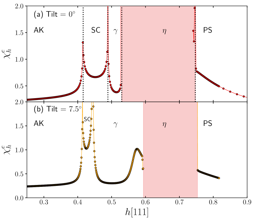
Figure 28: $\chi_{h}^{e}$ versus field for the KG ladder for (a) $h[111]$ field and (b) a field $\cos(\theta)h[111]+\sin(\theta)h[11-2]$ with $\theta=7.5^{\circ}$. The light red shading indicates regions where the iDMRG does not converge well. Results are from high precision iDMRG with unit cell of 60.

Appendix D The plaquette operator, $W_{p}$, in the AFM Kitaev region

The plaquette operator, $W_{p}$, introduced by Kitaev Kitaev (2006), is a crucial tool for characterizing the Kitaev spin liquid. On the honeycomb lattice $W_{p}$ is defined as a product of the six spins surrounding a hexagon in the lattice. In the setting of the KG ladder derived from a strip of the two-dimensional honeycomb lattice $W_{p}$ then corresponds to the 6 spins around 2 plaquettes of the ladder. Following the numbering of the sites on the ladder shown in Fig. 16 in the main text we then have:

$$W_{p}=\sigma_{1}^{y}\sigma_{2}^{z}\sigma_{3}^{x}\sigma_{4}^{x}\sigma_{5}^{z}\sigma_{6}^{y}.$$ (30)

Our results for $\langle W_{p}\rangle$ are shown in Fig. 27. At both the AFK and FM Kitaev points, $\phi=0$ and $\phi=\pi$ we have a flux-free state with $\langle W_{p}\rangle=1$ on all plaquettes. Away from these points $W_{p}$ can be different from 1. However, as can be seen in Fig. 27, $\langle W_{p}\rangle$ remains high throughout the AK phase only decreasing when the phase is exited. However, the different phases in the AFK region are only partly visible in Fig. 27. Interestingly, $\langle W_{p}\rangle$ is negative in the $\beta$ and $\eta$ phases shown as blue in Fig. 27.

Appendix E AF Kitaev point in Tilted Field

It is an interesting question if the phases found around the AF Kitaev point persist when the field direction is changed. In order to investigate this we have calculated $\chi_{h}^{e}$ in the presence of a field tilted slightly away from the [111] direction towards the [11-2] direction of the following form $\cos(\theta)h[111]+\sin(\theta)h[11-2]$ with $\theta=7.5^{\circ}$. Our results, obtained from iDMRG are shown in Fig. 28. In panel Fig. 28(a) we show for comparison our previous results for $\theta=0$ and in Fig. 28(b) for a tilted field with $\theta=7.5^{\circ}$. The AK, SC and $\gamma$ phases are still clearly present as is the transition to the polarized phase PS. However, the transition to the $\eta$ phase is in this case less well defined. In both panels the light red coloring indicates regions where the iDMRG does not converge well. Remarkably the critical fields for the AK-SC and $\eta$-PS transition appear almost unchanged by the tilt of the field.

References

- Kitaev (2006) A. Y. Kitaev, Anyons in an exactly solved model and beyond, Annals of Physics 321, 2 (2006).
- Khaliullin (2005) G. Khaliullin, Orbital order and fluctuations in mott insulators, Progress of Theoretical Physics Supplement 160, 155 (2005).
- Jackeli and Khaliullin (2009) G. Jackeli and G. Khaliullin, Mott insulators in the strong spin-orbit coupling limit: From Heisenberg to a quantum compass and Kitaev models, Phys. Rev. Lett. 102, 017205 (2009).
- Rau et al. (2014) J. G. Rau, E. K.-H. Lee, and H.-Y. Kee, Generic spin model for the honeycomb iridates beyond the Kitaev limit, Phys. Rev. Lett. 112, 077204 (2014).
- Plumb et al. (2014) K. W. Plumb, J. P. Clancy, L. J. Sandilands, V. V. Shankar, Y. F. Hu, K. S. Burch, H.-Y. Kee, and Y.-J. Kim, -RuCl3: A spin-orbit assisted mott insulator on a honeycomb lattice, Phys. Rev. B 90, 041112 (2014).
- Kim et al. (2015) H.-S. Kim, V. S. V., A. Catuneanu, and H.-Y. Kee, Kitaev magnetism in honeycomb -RuCl3 with intermediate spin-orbit coupling, Phys. Rev. B 91, 241110 (2015).
- Koitzsch et al. (2016) A. Koitzsch, C. Habenicht, E. Müller, M. Knupfer, B. Büchner, H. C. Kandpal, J. van den Brink, D. Nowak, A. Isaeva, and T. Doert, description of the honeycomb mott insulator , Physical Review Letters 117, 126403 (2016).
- Sandilands et al. (2016) L. J. Sandilands, Y. Tian, A. A. Reijnders, H.-S. Kim, Y.-J. Plumb, K. W. Kim, H.-Y. Kee, and K. S. Burch, Spin-orbit excitations and electronic structure of the putative kitaev magnet , Phys. Rev. B 93, 075144 (2016).
- Zhou et al. (2016) X. Zhou, H. Li, J. A. Waugh, S. Parham, H.-S. Kim, J. A. Sears, A. Gomes, H.-Y. Kee, Y.-J. Kim, and D. S. Dessau, Angle-resolved photoemission study of the kitaev candidate -rucl3, Physical Review B 94, 161106 (2016).
- Banerjee et al. (2016) A. Banerjee, C. A. Bridges, J.-Q. Yan, A. A. Aczel, L. Li, M. B. Stone, G. E. Granroth, M. D. Lumsden, Y. Yiu, J. Knolle, S. Bhattacharjee, D. L. Kovrizhin, R. Moessner, D. A. Tennant, D. G. Mandrus, and S. E. Nagler, Proximate Kitaev quantum spin liquid behaviour in a honeycomb magnet, Nature Materials 15, 733 (2016), article.
- Kim and Kee (2016) H.-S. Kim and H.-Y. Kee, Crystal structure and magnetism in -RuCl3: An ab initio study, Phys. Rev. B 93, 155143 (2016).
- Janssen et al. (2017) L. Janssen, E. C. Andrade, and M. Vojta, Magnetization processes of zigzag states on the honeycomb lattice: Identifying spin models for -RuCl3 and Na2IrO3, Phys. Rev. B 96, 064430 (2017).
- Winter et al. (2016) S. M. Winter, Y. Li, H. O. Jeschke, and R. Valentí, Challenges in design of Kitaev materials: Magnetic interactions from competing energy scales, Phys. Rev. B 93, 214431 (2016).
- Rau et al. (2016) J. G. Rau, E. K.-H. Lee, and H.-Y. Kee, Spin-orbit physics giving rise to novel phases in correlated systems: Iridates and related materials, Annual Review of Condensed Matter Physics 7, 195 (2016), https://doi.org/10.1146/annurev-conmatphys-031115-011319 .
- Winter et al. (2017) S. M. Winter, A. A. Tsirlin, M. Daghofer, J. van den Brink, Y. Singh, P. Gegenwart, and R. Valentí, Models and materials for generalized Kitaev magnetism, Journal of Physics: Condensed Matter 29, 493002 (2017).
- Hermanns et al. (2018) M. Hermanns, I. Kimchi, and J. Knolle, Physics of the Kitaev model: Fractionalization, dynamic correlations, and material connections, Annual Review of Condensed Matter Physics 9, 17 (2018), https://doi.org/10.1146/annurev-conmatphys-033117-053934 .
- Takagi et al. (2019) H. Takagi, T. Takayama, G. Jackeli, G. Khaliullin, and S. E. Nagler, Concept and realization of kitaev quantum spin liquids, Nature Reviews Physics 1, 264 (2019).
- Janssen and Vojta (2019) L. Janssen and M. Vojta, Heisenberg-kitaev physics in magnetic fields, Journal of Physics: Condensed Matter 31, 423002 (2019).
- Sandilands et al. (2015) L. J. Sandilands, Y. Tian, K. W. Plumb, Y.-J. Kim, and K. S. Burch, Scattering continuum and possible fractionalized excitations in -RuCl3, Phys. Rev. Lett. 114, 147201 (2015).
- Kasahara et al. (2018) Y. Kasahara, T. Ohnishi, Y. Mizukami, O. Tanaka, S. Ma, K. Sugii, N. Kurita, H. Tanaka, J. Nasu, Y. Motome, T. Shibauchi, and Y. Matsuda, Majorana quantization and half-integer thermal quantum Hall effect in a Kitaev spin liquid, Nature 559, 227 (2018).
- Johnson et al. (2015) R. D. Johnson, S. C. Williams, A. A. Haghighirad, J. Singleton, V. Zapf, P. Manuel, I. I. Mazin, Y. Li, H. O. Jeschke, R. Valentí, and R. Coldea, Monoclinic crystal structure of -RuCl3 and the zigzag antiferromagnetic ground state, Phys. Rev. B 92, 235119 (2015).
- Baek et al. (2017) S.-H. Baek, S.-H. Do, K.-Y. Choi, Y. S. Kwon, A. U. B. Wolter, S. Nishimoto, J. van den Brink, and B. Büchner, Evidence for a field-induced quantum spin liquid in -RuCl3, Phys. Rev. Lett. 119, 037201 (2017).
- Zheng et al. (2017) J. Zheng, K. Ran, T. Li, J. Wang, P. Wang, B. Liu, Z.-X. Liu, B. Normand, J. Wen, and W. Yu, Gapless spin excitations in the field-induced quantum spin liquid phase of -RuCl3, Phys. Rev. Lett. 119, 227208 (2017).
- Leahy et al. (2017) I. A. Leahy, C. A. Pocs, P. E. Siegfried, D. Graf, S.-H. Do, K.-Y. Choi, B. Normand, and M. Lee, Anomalous thermal conductivity and magnetic torque response in the honeycomb magnet , Phys. Rev. Lett. 118, 187203 (2017).
- Hentrich et al. (2018) R. Hentrich, A. U. B. Wolter, X. Zotos, W. Brenig, D. Nowak, A. Isaeva, T. Doert, A. Banerjee, P. Lampen-Kelley, D. G. Mandrus, S. E. Nagler, J. Sears, Y.-J. Kim, B. Büchner, and C. Hess, Unusual phonon heat transport in : Strong spin-phonon scattering and field-induced spin gap, Phys. Rev. Lett. 120, 117204 (2018).
- Lampen-Kelley et al. (2018) P. Lampen-Kelley, L. Janssen, E. C. Andrade, S. Rachel, J. Q. Yan, C. Balz, D. G. Mandrus, S. E. Nagler, and M. Vojta, Field-induced intermediate phase in -RuCl3: Non-coplanar order, phase diagram, and proximate spin liquid (2018), arXiv:1807.06192 .
- Janša et al. (2018) N. Janša, A. Zorko, M. Gomilšek, M. Pregelj, K. W. Krämer, D. Biner, A. Biffin, C. Rüegg, and M. Klanjšek, Observation of two types of fractional excitation in the kitaev honeycomb magnet, Nature Physics 14, 786 (2018).
- Banerjee et al. (2018) A. Banerjee, P. Lampen-Kelley, J. Knolle, C. Balz, A. A. Aczel, B. Winn, Y. Liu, D. Pajerowski, J. Yan, C. A. Bridges, A. T. Savici, B. C. Chakoumakos, M. D. Lumsden, D. A. Tennant, R. Moessner, D. G. Mandrus, and S. E. Nagler, Excitations in the field-induced quantum spin liquid state of -rucl3, npj Quantum Materials 3, 8 (2018).
- Shi et al. (2018) L. Y. Shi, Y. Q. Liu, T. Lin, M. Y. Zhang, S. J. Zhang, L. Wang, Y. G. Shi, T. Dong, and N. L. Wang, Field-induced magnon excitation and in-gap absorption in the kitaev candidate , Physical Review B 98, 094414 (2018).
- Widmann et al. (2019) S. Widmann, V. Tsurkan, D. A. Prishchenko, V. G. Mazurenko, A. A. Tsirlin, and A. Loidl, Thermodynamic evidence of fractionalized excitations in , Physical Review B 99, 094415 (2019).
- Sahasrabudhe et al. (2020) A. Sahasrabudhe, D. A. S. Kaib, S. Reschke, R. German, T. C. Koethe, J. Buhot, D. Kamenskyi, C. Hickey, P. Becker, V. Tsurkan, A. Loidl, S. H. Do, K. Y. Choi, M. Grüninger, S. M. Winter, Z. Wang, R. Valentí, and P. H. M. van Loosdrecht, High-field quantum disordered state in : Spin flips, bound states, and multiparticle continuum, Physical Review B 101, 140410 (2020).
- Wolter et al. (2017) A. U. B. Wolter, L. T. Corredor, L. Janssen, K. Nenkov, S. Schönecker, S.-H. Do, K.-Y. Choi, R. Albrecht, J. Hunger, T. Doert, M. Vojta, and B. Büchner, Field-induced quantum criticality in the Kitaev system -RuCl3, Phys. Rev. B 96, 041405 (2017).
- Yu et al. (2018) Y. J. Yu, Y. Xu, K. J. Ran, J. M. Ni, Y. Y. Huang, J. H. Wang, J. S. Wen, and S. Y. Li, Ultralow-temperature thermal conductivity of the kitaev honeycomb magnet across the field-induced phase transition, Phys. Rev. Lett. 120, 067202 (2018).
- Yamashita et al. (2020) M. Yamashita, N. Kurita, and H. Tanaka, Sample dependence of the half-integer quantized thermal hall effect in a kitaev candidate -rucl3 (2020), arXiv:2005.00798 [cond-mat.str-el] .
- Yadav et al. (2016) R. Yadav, N. A. Bogdanov, V. M. Katukuri, S. Nishimoto, J. Van Den Brink, and L. Hozoi, Kitaev exchange and field-induced quantum spin-liquid states in honeycomb -RuCl3, Scientific Reports 6, 37925 (2016).
- Chern et al. (2017) G.-W. Chern, Y. Sizyuk, C. Price, and N. B. Perkins, Kitaev-heisenberg model in a magnetic field: Order-by-disorder and commensurate-incommensurate transitions, Physical Review B 95, 144427 (2017).
- Zhu et al. (2018) Z. Zhu, I. Kimchi, D. N. Sheng, and L. Fu, Robust non-abelian spin liquid and a possible intermediate phase in the antiferromagnetic Kitaev model with magnetic field, Phys. Rev. B 97, 241110 (2018).
- Liang et al. (2018a) S. Liang, B.-S. He, Z.-Y. Dong, W. Chen, J.-X. Li, and Q.-H. Wang, Response and phase transition of a kitaev spin liquid in a local magnetic field, Physical Review B 98, 104410 (2018a).
- Gohlke et al. (2018) M. Gohlke, R. Moessner, and F. Pollmann, Dynamical and topological properties of the Kitaev model in a [111] magnetic field, Phys. Rev. B 98, 014418 (2018).
- Nasu et al. (2018) J. Nasu, Y. Kato, Y. Kamiya, and Y. Motome, Successive majorana topological transitions driven by a magnetic field in the Kitaev model, Phys. Rev. B 98, 060416 (2018).
- Ronquillo et al. (2019) D. C. Ronquillo, A. Vengal, and N. Trivedi, Signatures of magnetic-field-driven quantum phase transitions in the entanglement entropy and spin dynamics of the kitaev honeycomb model, Physical Review B 99, 140413 (2019).
- Liang et al. (2018b) S. Liang, M.-H. Jiang, W. Chen, J.-X. Li, and Q.-H. Wang, Intermediate gapless phase and topological phase transition of the kitaev model in a uniform magnetic field, Phys. Rev. B 98, 054433 (2018b).
- Liu and Normand (2018) Z.-X. Liu and B. Normand, Dirac and chiral quantum spin liquids on the honeycomb lattice in a magnetic field, Phys. Rev. Lett. 120, 187201 (2018).
- Kaib et al. (2019) D. A. S. Kaib, S. M. Winter, and R. Valentí, Kitaev honeycomb models in magnetic fields: Dynamical response and dual models, Physical Review B 100, 144445 (2019).
- Hickey and Trebst (2019) C. Hickey and S. Trebst, Gapless visons and emergent U(1) spin liquid in the kitaev honeycomb model: Complete phase diagram in tilted magnetic fields, Nature Communications 10, 530 (2019).
- Chern et al. (2020) L. E. Chern, R. Kaneko, H.-Y. Lee, and Y. B. Kim, Magnetic field induced competing phases in spin-orbital entangled kitaev magnets, Physical Review Research 2, 013014 (2020).
- Lee et al. (2020) H.-Y. Lee, R. Kaneko, L. E. Chern, T. Okubo, Y. Yamaji, N. Kawashima, and Y. B. Kim, Magnetic field induced quantum phases in a tensor network study of kitaev magnets, Nature Communications 11, 1639 (2020).
- Gohlke et al. (2020) M. Gohlke, L. E. Chern, H.-Y. Kee, and Y. B. Kim, Emergence of a nematic paramagnet via quantum order-by-disorder and pseudo-goldstone modes in kitaev magnets, arXiv:2003.11876 (2020).
- Gordon et al. (2019) J. S. Gordon, A. Catuneanu, E. S. Sørensen, and H.-Y. Kee, Theory of the field-revealed kitaev spin liquid, Nature Communications 10, 2470 (2019).
- Jiang et al. (2018) H.-C. Jiang, C.-Y. Wang, B. Huang, and Y.-M. Lu, Field induced quantum spin liquid with spinon fermi surfaces in the Kitaev model (2018), arXiv:1809.08247 .
- Zou and He (2020) L. Zou and Y.-C. He, Field-induced -chern-simons quantum criticalities in kitaev materials, Phys. Rev. Research 2, 013072 (2020).
- Patel and Trivedi (2019) N. D. Patel and N. Trivedi, Magnetic field-induced intermediate quantum spin liquid with a spinon fermi surface, Proceedings of the National Academy of Sciences 116, 12199 (2019), https://www.pnas.org/content/116/25/12199.full.pdf .
- Chaloupka and Khaliullin (2015) J. c. v. Chaloupka and G. Khaliullin, Hidden symmetries of the extended kitaev-heisenberg model: Implications for the honeycomb-lattice iridates , Phys. Rev. B 92, 024413 (2015).
- Kimchi and Coldea (2016) I. Kimchi and R. Coldea, Spin dynamics of counterrotating kitaev spirals via duality, Phys. Rev. B 94, 201110 (2016).
- Rousochatzakis and Perkins (2018) I. Rousochatzakis and N. B. Perkins, Magnetic field induced evolution of intertwined orders in the kitaev magnet , Phys. Rev. B 97, 174423 (2018).
- Stavropoulos et al. (2018) P. P. Stavropoulos, A. Catuneanu, and H.-Y. Kee, Counter-rotating spiral order in three-dimensional iridates: Signature of hidden symmetry in the kitaev- model, Phys. Rev. B 98, 104401 (2018).
- Sandvik (2007) A. W. Sandvik, Evidence for deconfined quantum criticality in a two-dimensional heisenberg model with four-spin interactions, Phys. Rev. Lett. 98, 227202 (2007).
- Senthil et al. (2004) T. Senthil, A. Vishwanath, L. Balents, S. Sachdev, and M. P. A. Fisher, Deconfined quantum critical points, Science 303, 1490 (2004), https://science.sciencemag.org/content/303/5663/1490.full.pdf .
- Yang et al. (2020a) W. Yang, A. Nocera, T. Tummuru, H.-Y. Kee, and I. Affleck, Phase diagram of the spin- kitaev-gamma chain and emergent su(2) symmetry, Phys. Rev. Lett. 124, 147205 (2020a).
- Karakonstantakis et al. (2013) G. Karakonstantakis, L. Liu, R. Thomale, and S. A. Kivelson, Correlations and renormalization of the electron-phonon coupling in the honeycomb hubbard ladder and superconductivity in polyacene, Phys. Rev. B 88, 224512 (2013).
- Feng et al. (2007a) X.-Y. Feng, G.-M. Zhang, and T. Xiang, Topological characterization of quantum phase transitions in a spin- model, Phys. Rev. Lett. 98, 087204 (2007a).
- Catuneanu et al. (2019) A. Catuneanu, E. S. Sørensen, and H.-Y. Kee, Nonlocal string order parameter in the kitaev-heisenberg ladder, Phys. Rev. B 99, 195112 (2019).
- Yang et al. (2020b) W. Yang, A. Nocera, E. S. Sørensen, H.-Y. Kee, and I. Affleck, Phase diagram of the spin- kitaev-gamma chain and emergent su(2) symmetry, arXiv:2004.06074 (2020b).
- Albuquerque et al. (2010) A. F. Albuquerque, F. Alet, C. Sire, and S. Capponi, Quantum critical scaling of fidelity susceptibility, Physical Review B 81, 064418 (2010).
- Li and Haldane (2008) H. Li and F. D. M. Haldane, Entanglement spectrum as a generalization of entanglement entropy: Identification of topological order in non-abelian fractional quantum hall effect states, Phys. Rev. Lett. 101, 010504 (2008).
- Catuneanu (2019) A. Catuneanu, Magnetic and topological aspects of spin liquid candidates with strong spin-orbit coupling, Ph. D, thesis (2019).
- Dagotto et al. (1992) E. Dagotto, J. Riera, and D. Scalapino, Superconductivity in ladders and coupled planes, Phys. Rev. B 45, 5744 (1992).
- Barnes et al. (1993) T. Barnes, E. Dagotto, J. Riera, and E. S. Swanson, Excitation spectrum of heisenberg spin ladders, Phys. Rev. B 47, 3196 (1993).
- Läuchli et al. (2003) A. Läuchli, G. Schmid, and M. Troyer, Phase diagram of a spin ladder with cyclic four-spin exchange, Phys. Rev. B 67, 100409 (2003).
- Kim et al. (2000) E. H. Kim, G. Fáth, J. Sólyom, and D. J. Scalapino, Phase transitions between topologically distinct gapped phases in isotropic spin ladders, Phys. Rev. B 62, 14965 (2000).
- Fáth et al. (2001) G. Fáth, O. Legeza, and J. Sólyom, String order in spin liquid phases of spin ladders, Phys. Rev. B 63, 134403 (2001).
- Rousochatzakis and Perkins (2017) I. Rousochatzakis and N. B. Perkins, Classical spin liquid instability driven by off-diagonal exchange in strong spin-orbit magnets, Phys. Rev. Lett. 118, 147204 (2017).
- Catuneanu et al. (2018) A. Catuneanu, Y. Yamaji, G. Wachtel, Y. B. Kim, and H.-Y. Kee, Path to stable quantum spin liquids in spin-orbit coupled correlated materials, npj Quantum Materials 3, 23 (2018).
- Feng et al. (2007b) X.-Y. Feng, G.-M. Zhang, and T. Xiang, Topological characterization of quantum phase transitions in a spin- model, Phys. Rev. Lett. 98, 087204 (2007b).
- Hastings (2007) M. B. Hastings, An area law for one-dimensional quantum systems, Journal of Statistical Mechanics: Theory and Experiment 2007, P08024 (2007).
- Gottesman and Hastings (2010) D. Gottesman and M. B. Hastings, Entanglement versus gap for one-dimensional spin systems, New Journal of Physics 12, 025002 (2010).
- Calabrese and Cardy (2004) P. Calabrese and J. Cardy, J. Stat. Mech. , 06002 (2004).
- Affleck and Ludwig (1991) I. Affleck and A. W. W. Ludwig, Universal noninteger “ground-state degeneracy” in critical quantum systems, Phys. Rev. Lett. 67, 161 (1991).