Deep Retrieval: Learning A Retrievable Structure for Large-Scale Recommendations

Abstract.

One of the core problems in large-scale recommendations is to retrieve top relevant candidates accurately and efficiently, preferably in sub-linear time. Previous approaches are mostly based on a two-step procedure: first learn an inner-product model, and then use some approximate nearest neighbor (ANN) search algorithm to find top candidates. In this paper, we present Deep Retrieval (DR), to learn a retrievable structure directly with user-item interaction data (e.g. clicks) without resorting to the Euclidean space assumption in ANN algorithms. DR’s structure encodes all candidate items into a discrete latent space. Those latent codes for the candidates are model parameters and learnt together with other neural network parameters to maximize the same objective function. With the model learnt, a beam search over the structure is performed to retrieve the top candidates for reranking. Empirically, we first demonstrate that DR, with sub-linear computational complexity, can achieve almost the same accuracy as the brute-force baseline on two public datasets. Moreover, we show that, in a live production recommendation system, a deployed DR approach significantly outperforms a well-tuned ANN baseline in terms of engagement metrics. To the best of our knowledge, DR is among the first non-ANN algorithms successfully deployed at the scale of hundreds of millions of items for industrial recommendation systems.

1. Introduction

Recommendation systems have gained great success in various commercial applications for decades. The objective of these systems is to return relevant items from a corpus based on user features and historical behaviors. One of the early successful techniques is the collaborative filtering (CF), based on the simple idea that similar users may prefer similar items. Item-based collaborative filtering (Item-CF) (Sarwar et al., 2001) extends this idea by considering the similarities between items and items, which lays the foundation for Amazon’s recommendation system (Linden et al., 2003).

In the Internet era, the size of users and items on popular content platforms rapidly grow to tens to hundreds of millions. The scalability, efficiency as well as accuracy, are all challenging problems in the design of modern recommendation systems. Recently, vector-based retrieval methods have been widely adopted. The main idea is to embed users and items in a latent vector space, and use the inner product of vectors to represent the preference between users and items. Representative vector embedding methods include matrix factorization (MF) (Mnih and Salakhutdinov, 2008; Koren et al., 2009), factorization machines (FM) (Rendle, 2010), DeepFM (Guo et al., 2017), Field-aware FM (FFM) (Juan et al., 2016), etc. However, when the number of items is large, the cost of brute-force computation of the inner products for all items can be prohibitive. Thus, approximate nearest neighbors (ANN) or maximum inner product search (MIPS) algorithms are usually used to retrieve top relevant items when the corpus is too large. Efficient MIPS or ANN algorithms include tree-based algorithms (Muja and Lowe, 2014; Houle and Nett, 2014), locality sensitive hashing (LSH) (Shrivastava and Li, 2014; Spring and Shrivastava, 2017), product quantization (PQ) (Jegou et al., 2010; Ge et al., 2013), hierarchical navigable small world graphs (HNSW) (Malkov and Yashunin, 2018), etc.

Despite their success in real world applications, vector-based methods with ANN or MIPS have two main disadvantages: (1) the inner product structure of user and item embeddings might not be sufficient to capture the complicated structure of user-item interactions (He et al., 2017). (2) ANN or MIPS is designed to approximate the learnt inner product model, not directly optimized for the user-item interaction data. As a solution, tree-based models (Zhu et al., 2018; Zhu et al., 2019; Zhuo et al., 2020) have been proposed to address these issues. One potential issue is of these methods is that each item is mapped to a leaf node in the tree, making the tree structure itself difficult to learn. Data available at the leaf level can be scarce and might not provide enough signal to learn a good tree structure at a finer level for a recommendation system with hundreds of millions of items. An efficient and easy-to-learn retrieval system is still very much needed for large-scale recommendations.

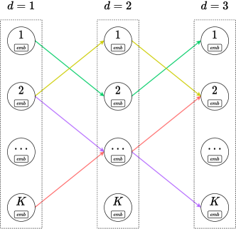
In this paper, we proposed Deep Retrieval (DR) to learn a retrievable structure in an end-to-end manner from data. DR uses a $K\times D$ matrix as shown in Fig. 1(a) for indexing, motivated by the ideas in Chen et al. (2018) and Van Den Oord et al. (2017), and we have introduced interdependence among the code in different $d\in\{1,...,D\}$. In this structure, we define a path $c$ as the forward index traverses over matrix columns. Each path is of length $D$ with index value range $\{1,2,\dots,K\}$. There are $K^{D}$ possible paths and each path can be interpreted as a cluster of items. We learn a probability distribution over the paths given the user inputs, jointly with a mapping from the items to the paths. In the serving stage, we use beam search to retrieve the most probable paths and the items associated with those paths. There are two major characteristics in designing the DR structure.

1. DR serves the purpose for “retrieval”, not ranking. Since there is no “leaf node” in DR’s structure, items within a path are indistinguishable for retrieval purpose, mitigating the data scarcity problem for ranking these items. DR can be easily scaled up to hundreds of millions items.

2. Each item is designed to be indexed by more than one path, meaning that two items can share some paths but differ in other paths. This design can be naturally realized using our probabilistic formulation of the DR model as we will show later. This multiple-to-multiple encoding scheme between items and paths differs significantly with the one-to-one mapping used in ealier designs of tree-based structures.

In training, the item paths are also model parameters and are learned together with other neural network parameters of the structure model using an expectation-maximization (EM) type algorithm (Dempster et al., 1977).

(a)

(b)

Figure 1. (a) Consider a structure with width $K=100$ and depth $D=3$, and an item encoded by a path of $[36,27,20]$. This path denotes that the item is assigned to the $(1,36)$, $(2,27)$, $(3,20)$ indices of the $K\times D$ matrix. In the figure, arrows with the same color form a path. Different paths could intersect with each other by sharing a common index in a layer. (b) Flow diagram of the process for constructing $p(c|x,\theta)$, the probability of path $c=[c_{1},c_{2},c_{3}]$ given input $x$.

Related Works

Here we briefly review some related works and discuss their connections to DR. Among numerous large-scale recommendation algorithms, the closest works to ours are the tree-based methods, including tree-based deep model (TDM) (Zhu et al., 2018), JTM (Zhu et al., 2019) , OTM (Zhuo et al., 2020) and AttentionXML (You et al., 2019). Tree-based methods map each item to a leaf node in a tree-based structure model and learn an objective function for the tree structure and the model parameters jointly. As discussed above, learning a good tree structure for hundreds of millions of items can be difficult.

Another line of research attempts to encode the candidates in a discrete latent space. Vector Quantised-Variational AutoEncoder(VQ-VAE) (Van Den Oord et al., 2017) uses a similar $K\times D$ embedding space to encode items, but focuses more on encoding data such as image or audio, whereas DR focuses on clustering items based on user-item interactions. HashRec (Kang and McAuley, 2019) and Merged-Averaged Classifiers via Hashing (Medini et al., 2019) use multi-index hash functions to encode candidate items in large recommendation systems. Compared to HashRec and MACH, DR uses a more complicated structure model with dependencies among layers and a different beam search based inference algorithm.

More complicated structure models have been used in extreme classification. LTLS (Jasinska and Karampatziakis, 2016) and W-LTLS (Evron et al., 2018) utilize directed acyclic graphs (DAG) as structure models. Probabilistic classifier chains (Dembczynski et al., 2010) are also used as structure models for multi-label classification. We note that the number of labels in these extreme classification applications is at most tens of thousands, whereas DR can be applied to industrial recommendation systems containing hundreds of millions of items.

Organization

The rest of the paper is organized as follows. In Section 2, we describe the structure model and its training objective function in detail. We then introduce a beam search algorithm to find candidate paths during the inference stage. In Section 3, we introduce the EM algorithm for training neural network parameters and paths of items jointly. In Section 4, we first demonstrate the performance of DR on two public datasets: MovieLens-20M and Amazon books. Experiment results show that DR can achieve almost the brute-force accuracy with sub-linear computational complexity. Moreover, in Section 5, we test the performance of DR on a live production recommendation system with hundreds of millions of users and items and show that it significantly outperforms a well-tuned ANN baseline in terms of engagement metrics in A/B test. In Section 6, we conclude the paper and discuss several possible future research directions.

2. Deep retrieval: Learning A Retrievable Structure from data

In this section, we introduce DR in detail. First, we establish its basic probability formulation. We then extend it to a multi-path mechanism that enables DR to capture multi-aspect properties of items. We then introduce a penalization design that prevents collapsing in allocating items to different paths. Next, we describe a beam search algorithm for retrieval. Finally, we present the multi-task joint training procedure of DR with a reranking model.

2.1. The DR Model

The basic model.

The basic DR model consists of $D$ layers, each with $K$ nodes. In each layer, we use a multi-layer perceptron (MLP) and $K$-class softmax to output a distribution over its $K$ nodes. Let $\mathcal{V}=\{1,\dots,V\}$ be the labels of all items and an item-to-path mapping $\pi:\mathcal{V}\to[K]^{D}$. Here a path is the forward index traverse over matrix columns as shown in Fig. 1(a). For simplicity, we assume that the mapping $\pi$ is given in this section (We will introduce the algorithm for learning the mapping $\pi$ later in Section 3.) In addition, we assume an item can only be mapped to one path for now and leave the multi-path setting to the next section.

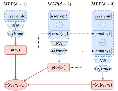
Given a pair of training sample $(x,y)$, which denotes a positive interaction (click, convert, like, etc.) between a user $x$ and an item $y$, as well as the path $c=(c_{1},c_{2},\dots,c_{D})$ associated with the item $y$, i.e. $\pi(y)=c$, the path probability $p(c|x,\theta)$ is constructed layer by layer as follows (see Fig. 1(b) for a flow chart),

• The first layer takes the user embedding ${\rm emb}(x)$ as input, and outputs a probability $p(c_{1}|x,\theta_{1})$ over the $K$ nodes of the first layer, based on parameters $\theta_{1}$ .

• From the second layer onward, we concatenate the user embedding ${\rm emb}(x)$ and the embeddings of all the previous layers ${\rm emb}(c_{d-1})$ (called path embeddings) as the input of MLP, which outputs $p(c_{d}|x,c_{1},\dots,c_{d-1},\theta_{d})$ over the $K$ nodes of layer $d$, based on parameters $\theta_{d}$.

• The probability of path $c$ given user $x$ is the product of the probabilities of all the layers’ outputs:

  (1) $$p(c|x,\theta)=\prod_{d=1}^{D}p(c_{d}|x,c_{1},\dots,c_{d-1},\theta_{d}).$$

Given a set of $N$ training samples $\{(x_{i},y_{i})\}_{i=1}^{N}$, the log likelihood function of the structure model is

$$\mathcal{Q}_{\rm str}(\theta,\pi)=\sum_{i=1}^{N}\log p(\pi(y_{i})|x_{i},\theta).$$

The size of the input vector of layer $d$ is the embedding size times $d$, and the size of the output vector is $K$. The parameters of layer $d$ have a size of $\Theta(Kd)$. The parameters $\theta$ contain the parameters $\theta_{d}$’s in all layers, as well as the path embeddings. The number of parameters in the entire model has an order of $\Theta(KD^{2})$, which is significantly smaller than the number of possible paths $K^{D}$ when $D\geq 2$.

Multi-path extension.

In tree-based deep models (Zhu et al., 2018; Zhu et al., 2019) as well as the structure model we introduced above, each item belongs to only one cluster/path, limiting the capacity of the model for expressing multi-aspect information in real data. For example, an item related to kebab could belong to a “food” cluster. An item related to flowers could belong to a “gift” cluster. However, an item related to chocolate or cakes could belong to both clusters in order to be recommended to users interested in either food or gifts. In real world recommendation systems, a cluster might not have an explicit meaning such as food or gifts, but this example motivates us to assign each item to multiple clusters. In DR, we allow each item $y_{i}$ to be assigned to $J$ different paths $\{c_{i,1},\dots,c_{i,J}\}$. Let $\pi:\mathcal{V}\to[K]^{D\times J}$ be the mapping from items to multiple paths. The multi-path structure objective is straightforwardly defined as

$$\mathcal{Q}_{\rm str}(\theta,\pi)=\sum_{i=1}^{N}\log\left(\sum_{j=1}^{J}p(c_{i,j}=\pi_{j}(y_{i})|x_{i},\theta)\right),$$

where the probability belonging to multiple paths is the summation of the probabilities belonging to individual paths.

Penalization on size of paths.

Directly optimizing $\mathcal{Q}_{\rm str}(\theta,\pi)$ w.r.t. the item-to-path mapping $\pi$ could fail to allocate different items into different paths (we did observe this in practice). In an extreme case, we could allocate all items into a single path and the probability of seeing this single path given any user $x$ is 1 as in Eq. 1. This is because there is only one available path to choose from. However, this will not help on retrieving the top candidates since there is no differentiation among the items. We must regulate the possible distribution of $\pi$ to ensure diversity. We introduce the following penalized likelihood function,

$$\mathcal{Q}_{\rm pen}(\theta,\pi)=\mathcal{Q}_{\rm str}(\theta,\pi)-\alpha\cdot\sum_{c\in[K]^{D}}f(|c|),$$

where $\alpha$ is the penalty factor, $|c|$ denotes the number of items allocated in path $c$ and $f$ is an increasing and convex function. A quadratic function $f(|c|)=|c|^{2}/2$ controls the average size of paths, and higher order polynomials penalize more on larger paths. In our experiments, we use $f(|c|)=|c|^{4}/4$.

2.2. Beam Search for Inference

In the inference stage, we want to retrieve items from the DR model, given user embeddings as input. To this end, we use the beam search algorithm (Reddy et al., 1977) to retrieve most probable paths. In each layer, the algorithm selects top $B$ nodes from all the successors of the selected nodes from the previous layer. Finally it returns $B$ top paths in the final layer. When $B=1$, this becomes the greedy search. In each layer, choosing top $B$ from $K\times B$ candidates has a time complexity of $O(KB\log B)$. The total complexity is $O(DKB\log B)$, which is sub-linear with respect to the total number of items $V$. We summarize the procedure in Algorithm 1.

Input: user $x$, model parameter $\theta$, beam size $B$.

Let $C_{1}=\{c_{1,1},\dots,c_{1,B}\}$ be top $B$ entries of $\{p(c_{1}|x,\theta):c_{1}\in\{1,\dots,K\}\}$.

for $d=2$ to $D$ do

       Let $C_{d}=\{(c_{1,1},\dots,c_{d,1}),\dots,(c_{1,B},\dots,c_{d,B})\}$ be the top $B$ entries of the set of all successors of $C_{d-1}$ defined as follows.

       $p(c_{1},\dots,c_{d-1}|x,\theta)p(c_{d}|x,c_{1},\dots,c_{d-1},\theta)$, where $(c_{1},\dots,c_{d-1})\in C_{d},c_{d}\in\{1,\dots,K\}$.

end for

Output: $C_{D}$, a set of $B$ paths.

Algorithm 1 Beam search algorithm

2.3. Multi-task Learning and Reranking with Softmax Models

The number of items returned by DR beam search is much smaller than the total number of items, but often not small enough to serve the user request, so we need to rank those retrieved items. However, since each path in DR can contain more than one item, it is not easy to differentiate these items using DR alone. We choose to tackle this by jointly training a DR model with a reranker:

$$\mathcal{Q}_{\rm softmax}=\sum_{i=1}^{N}\log p_{\rm softmax}(y=y_{i}|x_{i}),$$

where $p(y=y_{i}|x_{i})$ is a softmax model with output size $V$. This is trained with the sampled softmax algorithm. The final objective is given by $\mathcal{Q}=\mathcal{Q}_{\rm pen}+\mathcal{Q}_{\rm softmax}$. After performing a beam search to retrieval a set of candidate items, we rerank those candidates to obtain the final top candidates. Here we use a simple softmax model, but we can certainly replace it by a more complex one for better ranking performance.

3. Learning with the EM algorithm

In the previous section, we introduced the structure model in DR and its objective to be optimized. The objective is continuous with respect to the neural network parameters $\theta$, which can be optimized by any gradient-based optimizer. However, the objective involving the item-to-path mapping $\pi$ is discrete and can not be optimized by a gradient-based optimizer. As this mapping acts as the “latent clustering” of items, this motivates us to use an EM-style algorithm to optimize the mapping and other parameters jointly.

In general, the EM-style algorithm for DR is summarized as follows. We start with initializing mapping $\pi$ and other parameters randomly. Then at the $t^{\rm th}$ epoch,

1. E-step: for a fixed mapping $\pi^{(t-1)}$, optimize parameter $\theta$ using a gradient-based optimizer to maximize the structure objective $\mathcal{Q}_{\rm pen}(\theta,\pi^{(t-1)})$.

2. M-step: update mapping $\pi^{(t)}$ to maximize the same structure objective $\mathcal{Q}_{\rm pen}(\theta,\pi)$.

Since the E-step is similar to any standard stochastic optimization, we will focus on the M-step here. For simplicity, we first consider the objective $\mathcal{Q}_{\rm str}$ without the penalization. Given a user-item training pair $(x_{i},y_{i})$, let the set of paths associated with the item be $\{\pi_{1}(y_{i}),\dots,\pi_{J}(y_{i})\}$. For a fixed $\theta$, we can rewrite $\mathcal{Q}_{\rm str}(\theta,\pi)$ as

$$\mathcal{Q}_{\rm str}(\theta,\pi) =\sum_{i=1}^{N}\log\left(\sum_{j=1}^{J}p(\pi_{j}(y_{i})|x_{i},\theta)\right)\,$$

(2) $$=\sum_{v=1}^{V}\left(\sum_{i:y_{i}=v}\log\left(\sum_{j=1}^{J}p(\pi_{j}(v)|x_{i},\theta)\right)\right),$$

where the outer summation is over all items $v\in\mathcal{V}$ and the inner summation is over all appearances of item $v$ in the training set. We now consider maximizing the objective function over all possible mappings $\pi$. However, for an item $v$, there are $K^{D}$ number of possible paths so we could not enumerate it over all $\pi_{j}(v)$’s. We make the follow approximation to further simplify the problem since Eq. 2 is not easily solvable. We use an upper bound $\sum_{i=1}^{N}\log p_{i}\leq N(\log{\sum_{i=1}^{N}p_{i}}-\log N)$ to obtain

$$\mathcal{Q}_{\rm str}(\theta,\pi)\leq\overline{\mathcal{Q}}_{\rm str}(\theta,\pi)\,$$

$$=\sum_{v=1}^{V}\left(N_{v}\log\left(\sum_{j=1}^{J}\sum_{i:y_{i}=v}p(\pi_{j}(v)|x_{i},\theta)\right)-\log N_{v}\right),$$

where $N_{v}=\sum_{i=1}^{N}\mathbb{I}[i:y_{i}=v]$ denotes the number of occurrences of $v$ in the training set which is independent of the mapping. We define the following score function,

$$s[v,c]\triangleq\sum_{i:y_{i}=v}p(c|x_{i},\theta).$$

Intuitively, $s[v,c]$ can be understood as the accumulated importance score of allocating item $v$ to path $c$. In practice, it is impossible to retain all scores as the possible number of paths $c$ is exponentially large, so we only retain a subset of $S$ paths with largest scores through beam search and set the rest of the scores as $0$.

Remark on estimating $s[v,c]$ with streaming training.

Given the huge amount of continuously arriving data in real production recommendation systems, we typically have to use streaming training—processing the data only once ordered by their timestamps. So we choose to estimate scores $s[v,c]$ in a streaming fashion inspired by the approach in Metwally et al. (2005). The basic idea is to keep tracking a list of top $S$ important paths. For item $v$, suppose we have recorded score list $s[v,c_{1:S}]$. After we obtain a new list of scores, $s^{\prime}[v,c^{\prime}_{1:S}]$, from a new training instance containing $v$, we update the score list $s[v,c_{1:S}]$ as follows,

1. Let ${\rm min}\_{\rm score}=\min_{i}s[v,c_{i}]$.

2. Create a union set set $A=c_{1:S}\bigcup c^{\prime}_{1:S}$.

3. For each $c\in A$:

   1. If $c\in c_{1:S}$ and $c\in c^{\prime}_{1:S}$, set $s[v,c]\leftarrow\eta\ s[v,c]+s^{\prime}[v,c]$.

   2. If $c\notin c_{1:S}$ and $c\in c^{\prime}_{1:S}$, set $s[v,c]\leftarrow\eta\ {\rm min}\_{\rm score}+s^{\prime}[v,c]$.

   3. If $c\in c_{1:S}$ and $c\notin c^{\prime}_{1:S}$, set $s[v,c]\leftarrow\eta\ s[v,c]$.

4. Choose $S$ largest values of $s[v,c]$ from $c\in A$ to form the new score vector $s[v,c_{1:S}]$.

Figure 2. Illustration of the score updating process. $min(s)$ is used to increase the exploration of new paths in training. Blocks with the same colors indicate the same paths.

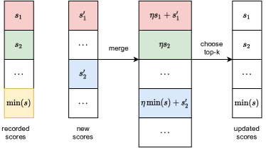
Here $\eta$ is a decay factor to account for the streaming estimation and we use $\eta=0.999$ in our experiments. As shown in Fig. 2, if the path (in red) appears both in the recorded list and the new list, we update the score by a discounted rolling sum. If the path (in green) appears only in the recorded list but not in the new list, we simply discount the score. If the path (in blue) appears only in the new list but not in the recorded list, we use ${\rm min}\_{\rm score}$ instead of $0$ as its score in the recorded list. This method increases the likelihood of exploring new paths in the streaming fashion, and we found it is important for the approach to work well.

Solving the M-step using coordinate descent.

Given score $s[v,c]$ estimated, now we consider the objective $\mathcal{Q}_{\rm pen}$ with penalization. This leads to the following surrogate function in the M-Step,

$$\arg\max_{\{\pi_{j}(v)\}_{j=1}^{J}} \sum_{v=1}^{V}\left(N_{v}\log\left(\sum_{j=1}^{J}s[v,\pi_{j}(v)]\right)-\log N_{v}\right)\,$$

$$-\alpha\cdot\sum_{c\in[K]^{D}}f(|c|).$$

Notice that there is no closed-form solution for this maximization problem. Hence, we utilize the coordinate descent algorithm, by optimizing over the path assignments for item $v$ while fixing the assignments of all other items. Notice that the term $-\log N_{v}$ is irrelevant to $\pi_{j}(v)$ and hence can be dropped. The partial objective function related to item $v$ can be simplified as

$$\arg\max_{\{\pi_{j}(v)\}_{j=1}^{J}}N_{v}\log\left(\sum_{j=1}^{J}s[v,\pi_{j}(v)]\right)-\alpha\sum_{j=1}^{J}f(|\pi_{j}(v)|).$$

Now we choose the path assignments $\{\pi_{1}(v),\dots,\pi_{j}(v)\}$ step by step. At step $i$, the incremental gain of the objective function by choosing $c=\pi_{i}(v)$ is given as follows:

$$N_{v}\left(\log(\sum_{j=1}^{i-1}s[v,\pi_{j}(v)]+s[v,c])-\log(\sum_{j=1}^{i-1}s[v,\pi_{j}(v)])\right)\,$$

$$-\alpha\left(f(|c|+1)-f(|c|)\right).$$

By keeping track of the partial sum $\sum_{j=1}^{i-1}s[v,\pi_{j}(v)]$ and the size of paths $|c|$, we greedily choose the path with the largest incremental gain. The details of the coordinate descent algorithm is given in Algorithm 2. In practice, three to five iterations are enough to ensure the algorithm converges. The time complexity grows linearly with vocabulary size $V$, multiplicity of paths $J$ as well as number of candidate paths $S$.

Input: Score functions $\log s[v,c]$. Number of iterations $T$.

Initialization: Set $|c|=0$ for all paths $c$.

for $t=1$ to $T$ do

       for all items $v$ do

             Initialize the partial sum, ${\rm sum}\leftarrow 0$.

             for $j=1$ to $J$ do

                   if $t>1$ then

                         $|\pi^{(t-1)}_{j}(v)|\leftarrow|\pi^{(t-1)}_{j}(v)|-1$. (Reset path size for assignments from last iteration).

                   end if

                  for all candidate paths $c$ of item $v$ such that $c\not\in\{\pi_{l}^{(t)}(v)\}_{l=1}^{j-1}$ do

                         Compute incremental gain of objective function

$$\Delta s[v,c]=N_{v}\left(\log(s[v,c]+{\rm sum})-\log({\rm sum})\right)-\alpha\left(f(|c|+1)-f(|c|)\right).$$

                   end for

                  $\pi_{j}^{(t)}(v)\leftarrow\arg\max_{c}\Delta s[v,c]$.

                   ${\rm sum}\leftarrow{\rm sum}+s[v,\pi_{j}^{(t)}(v)]$ (Update partial sum).

                   $|\pi_{j}^{(t)}(v)|\leftarrow|\pi_{j}^{(t)}(v)|+1$ (Update path size).

                  

             end for

            

       end for

      

end for

Output: path assignments $\{\pi^{(T)}_{j}(v)\}_{j=1}^{J}$.

Algorithm 2 Coordinate descent algorithm for penalized path assignment.

4. Experiments on public datasets

In this section, we study the performance of DR on two public recommendation datasets: MovieLens-20M (Harper and Konstan, 2015) and Amazon books (He and McAuley, 2016; McAuley et al., 2015). We compare the performance of DR with brute-force algorithm, as well as several other recommendation baselines including tree-based models TDM (Zhu et al., 2018) and JTM (Zhu et al., 2019). At the end of this section, we investigate the role of important hyperparameters in DR.

4.1. Datasets and Metrics

MovieLens-20M. This dataset contains rating and free-text tagging activities from a movie recommendation service called MovieLens. We use the 20M subset which were created by the behaviors of 138,493 users between 1995 and 2015. Each user-movie interaction contains a used-id, a movie-id, a rating between 1.0 to 5.0, as well as a timestamp.

In order to make a fair comparison, we exactly follow the same data pre-processing procedure as TDM. We only keep records with rating higher or equal to 4.0, and only keep users with at least ten reviews. After pre-processing, the dataset contains 129,797 users, 20,709 movies and 9,939,873 interactions. Then we randomly sample 1,000 users and corresponding records to construct the validation set, another 1,000 users to construct the test set, and other users to construct the training set. For each user, the first half of the reviews according to the timestamp are used as historical behavior features and the latter half are used as ground truths to be predicted.

Amazon books. This dataset contains user reviews of books from Amazon, where each user-book interaction contains a user-id, an item-id, and the corresponding timestamp. Similar to MovieLens-20M, we follow the same pre-processing procedure as JTM. The dataset contains 294,739 users, 1,477,922 items and 8,654,619 interactions. Please note that Amazon books dataset has much more items but sparser interactions than MovieLens-20M. We randomly sample 5,000 users and corresponding records as the test set, another 5,000 users as the validation set and other users as the training set. The construction procedures of behavior features and ground truths are the same as in MovieLens-20M.

Metrics. We use precision, recall and F-measure as metrics to evaluate the performance for each algorithm. The metrics are computed for each user individually, and averaged without weight across users, following the same setting as both TDM and JTM. We compute the metrics by retrieving top $10$ and $200$ items for each user in MovieLens-20M and Amazon books respectively.

Model and training. Since the dataset is split in a way such that the users in the training set, validation set and test set are disjoint, we drop the user-id and only use the behavior sequence as input for DR. The behavior sequence is truncated to length of 69 if it is longer than 69, and filled with a placeholder symbol if it is shorter than 69. A recurrent neural network with GRU is utilized to project the behavior sequence onto a fixed dimension embedding as the input of DR. We adopt the multi-task learning framework, and rerank the items in the recalled paths by a softmax reranker. We train the embeddings of DR and softmax jointly for the initial two epochs, freeze the embeddings of softmax and train the embeddings of DR for two more epochs. The reason is to prevent overfitting of the softmax model. In the inference stage, the number of items retrieved from beam search is not fixed due to the differences of path sizes, but the variance is not large. Empirically we control the beam size such that the number of items from beam search is 5 to 10 times the number of finally retrieved items.

Table 1. Comparison of precision@10, recall@10 and F-measure@10 for DR, brute-force retrieval and other recommendation algorithms on MovieLens-20M.

Algorithm	Precision@10	Recall@10	F-measure@10
Item-CF	8.25%	5.66%	5.29%
YouTube DNN	11.87%	8.71%	7.96%
TDM (best)	14.06%	10.55%	9.49%
DR	20.58 $\pm$ 0.47%	10.89 $\pm$ 0.32%	12.32 $\pm$ 0.36%
Brute-force	20.70 $\pm$ 0.16%	10.96 $\pm$ 0.32%	12.38 $\pm$ 0.32%

Table 2. Comparison of precision@200, recall@200 and F-measure@200 for DR, brute-force retrieval and other recommendation algorithms on Amazon Books.

Algorithm	Precision@200	Recall@200	F-measure@200
Item-CF	0.52%	8.18%	0.92%
YouTube DNN	0.53%	8.26%	0.93%
TDM (best)	0.56%	8.57%	0.98%
JTM	0.79%	12.45%	1.38%
DR	0.95 $\pm$ 0.01%	13.74 $\pm$ 0.14%	1.63 $\pm$ 0.02%
Brute-force	0.95 $\pm$ 0.01%	13.75 $\pm$ 0.10%	1.63 $\pm$ 0.02%

4.2. Empirical Results

We compare the performance of DR with the following algorithms: Item-CF (Sarwar et al., 2001), YouTube product DNN (Covington et al., 2016), TDM and JTM. We directly use the numbers of Item-CF, Youtube DNN, TDM and JTM from TDM and JTM papers for fair comparison. Among the different variants of TDM presented, we pick the one with best performance. The result of JTM is only available for Amazon books. We also compare DR with brute-force retrieval algorithm, which directly computes the inner-product of user embedding and all the item embeddings learnt in the softmax model and returns the top $K$ items. The brute-force algorithm is usually computationally prohibitive in practical large recommendation systems, but can be used as an upper bound for small dataset for inner-product based models.

Table 3. Comparison of inference time for DR and brute-force retrieval on Amazon Books.

Deep Retrieval	0.266 ms per instance
Brute-force	1.064 ms per instance

Table 1 shows the performance of DR compared to other algorithms and brute-force for MovieLens-20M. Table 2 shows the results for Amazon books. For DR and brute-force, we independently train the same model for 5 times and compute the mean and standard deviation of each metric. Results are as follows.

• DR performs better than other methods including tree-based retrieval algorithms such as TDM and JTM.

• The performance of DR is very close to or on par with the performance of brute-force method, which can be thought as an upper bound of the performance of vector-based methods such as Deep FM and HNSW. However, the inference speed of DR is 4 times faster than brute-force in Amazon books dataset (see Table 3).

4.3. Sensitivity of Hyperparameters

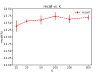
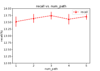
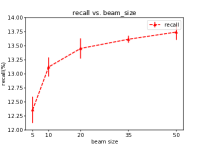
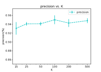
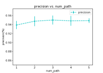
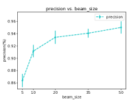
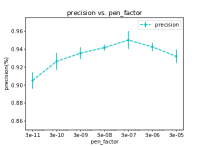
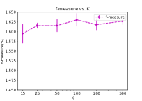
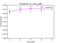
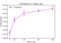
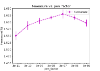
DR introduces some key hyperparameters which may affect the performance dramatically, including the width of the structure model $K$, depth of model $D$, number of multiple paths $J$, beam size $B$ and penalty factor $\alpha$. In the MovieLens-20M experiment, we choose $K=50$, $D=3$, $B=25$, $J=3$ and $\alpha=3\times 10^{-5}$. In the Amazon books experiment, we choose $K=100$, $D=3$, $B=50$, $J=3$ and $\alpha=3\times 10^{-7}$. Using the Amazon books dataset, we show the role of these hyperparameters and see how they may affect the performance. We present how the recall@200 change as these hyperparameters change in Fig. 3. We keep the value of other hyperparameters unchanged when varying one hyperparameter. Precision@200 and F-measure@200 follow similar trends are shown in Fig. 4 and Fig. 5.

Figure 3. Relationship between recall@200 in Amazon Books experiment and model width $K$, number of paths $J$, beam size $B$ and penalty factor $\alpha$, respectively.

Figure 4. Relationship between precision@200 in Amazon Books experiment and model width $K$, number of paths $J$, beam size $B$ and penalty factor $\alpha$, respectively.

Figure 5. Relationship between F-measure@200 in Amazon Books experiment and model width $K$, number of paths $J$, beam size $B$ and penalty factor $\alpha$, respectively.

Table 4. Comparison of performance for different model depth $D$ on Amazon Books.

$(K,D)$	Precision @ 200	Recall @ 200	F-measure @ 200
(100, 2)	0.93%	13.34%	1.59%
(100, 3)	0.95%	13.74%	1.63%
(100, 4)	0.95%	13.67%	1.63%
(1000, 2)	0.95%	13.68%	1.62%

Table 5. Relationship between the size of the path with most items (top path size) and penalty factor $\alpha$.

Penalty factor $\alpha$	3e-9	3e-8	3e-7	3e-6
Top path size	1948 $\pm$ 30	956 $\pm$ 29	459 $\pm$ 13	242 $\pm$ 1

• Width of model $K$ controls the overall capacity of the model. If $K$ is small, the number of clusters is small for all the items; if $K$ is big, the time complexity of training and inference stages grow linearly with $K$. Moreover, large $K$ may increase the possibility of overfitting. An appropriate $K$ should be chosen depending on the size of the corpus.

• Depth of model $D$. Using $D=1$ is obviously not a good idea since it fails to capture dependency among layers. In Table 4, we investigate the result for $D=2,3$ and $4$ for Amazon books dataset and conclude that (1) using $D=2$ with the same $K$ would hurt performance; (2) using $D=4$ with the same $K$ would not help. (3) Models with the same number of possible paths ($K=1000,D=2$ and $K=100,D=3$) have similar performance. However the number of parameters is of order $KD^{2}$, so a deeper model can achieve the same performance with fewer parameters. As a trade-off between model performance and memory usage, we choose $D=3$ in all experiments.

• Number of paths $J$ enables the model to express multi-aspect information of candidate items. The performance is the worst when $J=1$, and keeps increasing as $J$ increases. Large $J$ may not affect the performance, but the time complexity for training grows linearly with $J$. In practice, choosing $J$ between 3 and 5 is recommended.

• Beam size $B$ controls the number of candidate paths to be recalled. Larger $B$ leads a better performance as well as heavier computation in the inference stage. Notice that greedy search is a special case when $B=1$, whose performance is worse than beam search with larger $B$.

• Penalty factor $\alpha$ controls the number of items in each path. The best performance is achieved when $\alpha$ falls in a certain range. From table 5, we conclude that smaller $\alpha$ leads to a larger path size hence heavier computation in the reranking stage. Beam size $B$ and penalty factor $\alpha$ should be appropriately chosen as a trade off between model performance and inference speed.

Overall, we can see that DR is fairly stable to hyperparameters since there is a wide range of hyperparameters which leads to near-optimal performances.

5. Live experiments

In this section, we show how DR works in real production systems. To the best of our knowledge, DR is among the first non-ANN algorithms successfully deployed at the scale of hundreds of millions of items for industrial recommendation systems.

While the results on public datasets in the last section shed light upon the basic behavior of the DR models, it is more important to understand if it could improve user experiences for real recommendation systems in industrial environments. These systems are much more complicated and difficult to improve due to sheer volume of the data (user-generated contents, UGC) and their dynamic nature—there are new items uploaded almost every second.

Since the number of items in our system is usually in the order of hundreds of millions, making the full-scale fine ranking a difficult task. Thus, an industrial-scale recommendation system usually consists of several stages as shown in the YouTube recommendation paper (Covington et al., 2016). At minimal, the system has two stages: candidate generation and fine-ranking. Here fine-ranking stage usually uses a more complex model with additional features that are computationally intractable in the candidate generation stage. Thus fine ranking usually handles only hundreds of items for each user request. DR works as the one of candidate generation components. Fig. 6 shows the illustrative diagram of this process. In practice, multiple candidate generation sources are used at the same time to produce a diverse set of candidates for the fine-ranking stage.

Figure 6. An illustrative diagram to show how to use DR in an industrial recommendation system.

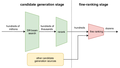
Our experimental platform is one of the largest in the industry with hundreds of millions of users and items. In our system, items are short videos. For this particular DR experiment, the labels are generated to indicate whether a user has finished watching the video or not. The baseline candidate generation method used Field-aware Factorization Machine (FFM) (Juan et al., 2016) to learn the user and item embeddings and followed by HNSW (Malkov and Yashunin, 2018) for approximate nearest neighbor search. This baseline was extensively tuned to maximize the user experiences on the platform. Slightly different from the use of softmax for reranking on public datasets for DR, the re-ranking model we use here is a logistic regression model. Previous attempts of using softmax in the production did not result in meaningful improvements. The reranking model architecture is the same for both HNSW and DR.

We report the performance of DR in AB test in Table 6. DR enjoys a significant gain in key metrics, including video finish rate, app view time and second day retention, over the baseline model. All improvements are statistically significant. This is likely because the end-to-end training of DR aligns the learning of the user embeddings and the retrievable structure under the same objective function directly from user-item interactions. So the clustering of DR contains more user-behavior information of candidate items. We also found that DR is more friendly to less popular videos or less popular creators, and the AB test shows that much more of such videos are recommended to the end users. This is beneficial to the platform’s creator ecosystem. We believe the reason is as follows. Within each path in the DR structure, items are indistinguishable and this allows the less popular items to be retrieved as long as they share some similar behaviors with popular ones. Last but not least, DR is naturally suitable for streaming training, and the time to build the structure for retrieval is much less than HNSW since there is no computation of any user or item embeddings involved in DR’s M-step. It takes about 10 minutes to process the total items with a multi-thread CPU implementation. In industrial recommendation systems like ours, these improvements are substantial. This experiment shows the advantage of DR in large-scale recommendation systems.

Table 6. Live experiment results on different engagement metrics.

Metric	Relative improvement of DR
Video finish rate	+3.0%
App view time	+0.87%
Second day retention	+0.036%

6. Conclusion and discussion

In this paper, we have proposed Deep Retrieval, an end-to-end learnable structure model for large-scale recommendation systems. DR uses an EM-style algorithm to learn the model parameters and paths of items jointly. Experiments have shown that DR performs well compared with brute-force baselines in two public recommendation datasets as well as live production environments with hundreds of millions of users and items. There are several future research directions based on the current model design. Firstly, the structure model defines the probability distribution on paths only based on user side information. A useful idea would be how to incorporate item side information more directly into the DR model. Secondly, in the structure model, we only make use of positive interactions such as click, convert or like between user and item. Negative interactions such as non-click, dislike or unfollow should also be considered in future work to improve the model performance. Finally, we currently use a simple dot-product type of models as a reranker and we plan to use a more complex model in the future.

References

- (1)
- Chen et al. (2018) Ting Chen, Martin Renqiang Min, and Yizhou Sun. 2018. Learning K-way D-dimensional discrete codes for compact embedding representations. arXiv preprint arXiv:1806.09464 (2018).
- Covington et al. (2016) Paul Covington, Jay Adams, and Emre Sargin. 2016. Deep neural networks for youtube recommendations. In Proceedings of the 10th ACM conference on recommender systems. 191–198.
- Dembczynski et al. (2010) Krzysztof Dembczynski, Weiwei Cheng, and Eyke Hüllermeier. 2010. Bayes optimal multilabel classification via probabilistic classifier chains. In International Conference on Machine Learning (ICML).
- Dempster et al. (1977) Arthur P Dempster, Nan M Laird, and Donald B Rubin. 1977. Maximum likelihood from incomplete data via the EM algorithm. Journal of the Royal Statistical Society: Series B (Methodological) 39, 1 (1977), 1–22.
- Evron et al. (2018) Itay Evron, Edward Moroshko, and Koby Crammer. 2018. Efficient loss-based decoding on graphs for extreme classification. (2018), 7233–7244.
- Ge et al. (2013) Tiezheng Ge, Kaiming He, Qifa Ke, and Jian Sun. 2013. Optimized product quantization. IEEE transactions on pattern analysis and machine intelligence 36, 4 (2013), 744–755.
- Guo et al. (2017) Huifeng Guo, Ruiming Tang, Yunming Ye, Zhenguo Li, and Xiuqiang He. 2017. DeepFM: a factorization-machine based neural network for CTR prediction. arXiv preprint arXiv:1703.04247 (2017).
- Harper and Konstan (2015) F Maxwell Harper and Joseph A Konstan. 2015. The movielens datasets: History and context. Acm transactions on interactive intelligent systems (tiis) 5, 4 (2015), 1–19.
- He and McAuley (2016) Ruining He and Julian McAuley. 2016. Ups and downs: Modeling the visual evolution of fashion trends with one-class collaborative filtering. In proceedings of the 25th international conference on world wide web. 507–517.
- He et al. (2017) Xiangnan He, Lizi Liao, Hanwang Zhang, Liqiang Nie, Xia Hu, and Tat-Seng Chua. 2017. Neural collaborative filtering. In Proceedings of the 26th international conference on world wide web. 173–182.
- Houle and Nett (2014) Michael E Houle and Michael Nett. 2014. Rank-based similarity search: Reducing the dimensional dependence. IEEE transactions on pattern analysis and machine intelligence 37, 1 (2014), 136–150.
- Jasinska and Karampatziakis (2016) Kalina Jasinska and Nikos Karampatziakis. 2016. Log-time and log-space extreme classification. arXiv preprint arXiv:1611.01964 (2016).
- Jegou et al. (2010) Herve Jegou, Matthijs Douze, and Cordelia Schmid. 2010. Product quantization for nearest neighbor search. IEEE transactions on pattern analysis and machine intelligence 33, 1 (2010), 117–128.
- Juan et al. (2016) Yuchin Juan, Yong Zhuang, Wei-Sheng Chin, and Chih-Jen Lin. 2016. Field-aware factorization machines for CTR prediction. In Proceedings of the 10th ACM Conference on Recommender Systems. 43–50.
- Kang and McAuley (2019) Wang-Cheng Kang and Julian McAuley. 2019. Candidate generation with binary codes for large-scale top-n recommendation. In Proceedings of the 28th ACM International Conference on Information and Knowledge Management. 1523–1532.
- Koren et al. (2009) Yehuda Koren, Robert Bell, and Chris Volinsky. 2009. Matrix factorization techniques for recommender systems. Computer 42, 8 (2009), 30–37.
- Linden et al. (2003) Greg Linden, Brent Smith, and Jeremy York. 2003. Amazon. com recommendations: Item-to-item collaborative filtering. IEEE Internet computing 7, 1 (2003), 76–80.
- Malkov and Yashunin (2018) Yury A Malkov and Dmitry A Yashunin. 2018. Efficient and robust approximate nearest neighbor search using hierarchical navigable small world graphs. IEEE transactions on pattern analysis and machine intelligence (2018).
- McAuley et al. (2015) Julian McAuley, Christopher Targett, Qinfeng Shi, and Anton Van Den Hengel. 2015. Image-based recommendations on styles and substitutes. In Proceedings of the 38th International ACM SIGIR Conference on Research and Development in Information Retrieval. 43–52.
- Medini et al. (2019) Tharun Kumar Reddy Medini, Qixuan Huang, Yiqiu Wang, Vijai Mohan, and Anshumali Shrivastava. 2019. Extreme classification in log memory using count-min sketch: A case study of amazon search with 50m products. In Advances in Neural Information Processing Systems. 13265–13275.
- Metwally et al. (2005) Ahmed Metwally, Divyakant Agrawal, and Amr El Abbadi. 2005. Efficient computation of frequent and top-k elements in data streams. In International conference on database theory. Springer, 398–412.
- Mnih and Salakhutdinov (2008) Andriy Mnih and Russ R Salakhutdinov. 2008. Probabilistic matrix factorization. In Advances in Neural Information Processing Systems. 1257–1264.
- Muja and Lowe (2014) Marius Muja and David G Lowe. 2014. Scalable nearest neighbor algorithms for high dimensional data. IEEE transactions on pattern analysis and machine intelligence 36, 11 (2014), 2227–2240.
- Reddy et al. (1977) D Raj Reddy et al. 1977. Speech understanding systems: A summary of results of the five-year research effort. Department of Computer Science. Camegie-Mell University, Pittsburgh, PA 17 (1977).
- Rendle (2010) Steffen Rendle. 2010. Factorization machines. In 2010 IEEE International Conference on Data Mining. IEEE, 995–1000.
- Sarwar et al. (2001) Badrul Sarwar, George Karypis, Joseph Konstan, and John Riedl. 2001. Item-based collaborative filtering recommendation algorithms. In Proceedings of the 10th international conference on World Wide Web. 285–295.
- Shrivastava and Li (2014) Anshumali Shrivastava and Ping Li. 2014. Asymmetric LSH (ALSH) for sublinear time maximum inner product search (MIPS). In Advances in Neural Information Processing Systems. 2321–2329.
- Spring and Shrivastava (2017) Ryan Spring and Anshumali Shrivastava. 2017. A New Unbiased and Efficient Class of LSH-Based Samplers and Estimators for Partition Function Computation in Log-Linear Models. arXiv preprint arXiv:1703.05160 (2017).
- Van Den Oord et al. (2017) Aaron Van Den Oord, Oriol Vinyals, et al. 2017. Neural discrete representation learning. (2017), 6306–6315.
- You et al. (2019) Ronghui You, Zihan Zhang, Ziye Wang, Suyang Dai, Hiroshi Mamitsuka, and Shanfeng Zhu. 2019. Attentionxml: Label tree-based attention-aware deep model for high-performance extreme multi-label text classification. In Advances in Neural Information Processing Systems. 5820–5830.
- Zhu et al. (2019) Han Zhu, Daqing Chang, Ziru Xu, Pengye Zhang, Xiang Li, Jie He, Han Li, Jian Xu, and Kun Gai. 2019. Joint optimization of tree-based index and deep model for recommender systems. In Advances in Neural Information Processing Systems. 3973–3982.
- Zhu et al. (2018) Han Zhu, Xiang Li, Pengye Zhang, Guozheng Li, Jie He, Han Li, and Kun Gai. 2018. Learning tree-based deep model for recommender systems. In Proceedings of the 24th ACM SIGKDD International Conference on Knowledge Discovery & Data Mining. 1079–1088.
- Zhuo et al. (2020) Jingwei Zhuo, Ziru Xu, Wei Dai, Han Zhu, Han Li, Jian Xu, and Kun Gai. 2020. Learning optimal tree models under beam search. arXiv:2006.15408 [stat.ML]