Towards Dense People Detection with Deep Learning and Depth images

Abstract

This paper proposes a DNN-based system that detects multiple people from a single depth image. Our neural network processes a depth image and outputs a likelihood map in image coordinates, where each detection corresponds to a Gaussian-shaped local distribution, centered at the person’s head. The likelihood map encodes both the number of detected people and their 2D image positions, and can be used to recover the 3D position of each person using the depth image and the camera calibration parameters. Our architecture is compact, using separated convolutions to increase performance, and runs in real-time with low budget GPUs. We use simulated data for initially training the network, followed by fine tuning with a relatively small amount of real data. We show this strategy to be effective, producing networks that generalize to work with scenes different from those used during training. We thoroughly compare our method against the existing state-of-the-art, including both classical and DNN-based solutions. Our method outperforms existing methods and can accurately detect people in scenes with significant occlusions.

1 Introduction

People detection and localization from cameras has received a great deal of attention from the scientific community recently, due to its multiple applications in different areas, such as security, video surveillance [59, 41] or healthcare [36, 61, 21]. However, it remains an open problem, and presents several challenging tasks [64, 65], especially in crowded scenes.

Early people detection methods used RGB images captured from a mainly frontal viewpoint. Methods such as  [44, 9, 30, 4, 1] use traditional computer vision algorithms, such as appearance models in [44] or classic face detection in [9]. These approaches obtained good results in controlled spaces but struggle with the presence of partial occlusions, motion blur and low resolution images.

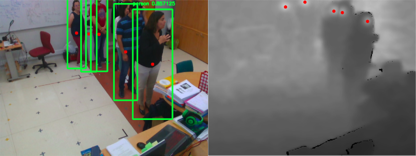
Deep Neural Networks (DNN) have greatly improved the state-of-the-art in several critical computer vision applications, such as object detection [45], semantic segmentation [7], classification [49] or activity recognition [26, 63]. Similarly, DNN-based people detection methods using RGB data [6, 15, 22] have considerably improved over the classical algorithms. However, DNN-based methods also have significant drawbacks, such as the large amount of labeled data needed for training and the requirement of dedicated processing units to run and train the network. Besides, recent DNN-based methods still present low accuracy in highly cluttered scenes (see Fig. 1).

People detection using depth images is a less popular topic in the literature, mainly because depth cameras are not as widely available as RGB cameras. Nonetheless, using depth images has significant advantages: 1) Depth images naturally disambiguate objects at different depths, which helps to process occlusions in crowded scenes. 2) Depth information is less complex than RGB information as it is not affected by appearance or light changes. 3) Once detected in the image, positions of people in 3D are directly available using depth information, which is a desirable feature in many applications.

There exist several depth-based people detection methods in the literature, and some of them also include RGB information. Recent DNN-based approaches obtain the best detection results in this category. However, they bear important limitations. Some methods are specific to zenithal viewpoints [12, 40, 19, 68], which reduces occlusions and makes the problem less ambiguous, but limits the field-of-view. Others use a conventional frontal viewpoint [23, 68], which covers a wider range of applications. [23, 68] use a region proposal method to detect candidates, and a classifier to select the positive regions that correspond to a person. This strategy is not optimal, especially for densely populated scenes, and it is not efficient, as its complexity depends on the number of possible candidates detected in the image.

This paper proposes a new DNN-based approach, that we call PD3net, for detecting multiple people from a single depth image acquired using a camera in an elevated frontal position, see Fig. 1. Our method has the following contributions: 1) Our network architecture is fully convolutional and very efficient by using spatially separable convolutions. It runs in real-time with low-cost GPU and CPU architectures. 2) We train the neural network end-to-end with synthetically generated depth images and then we fine-tune the network with a small number of annotated real images. The paper shows that this strategy leads to accurate and generalistic detectors that work well in general scenes. 3) Our method recovers a dense likelihood map that effectively detects multiple people in crowded scenes (see Fig. 1). 4) We outperform the existing state-of-the-art, including both classical and DNN-based approaches. 5) The proposed method works with different cameras and depth sensing technologies. 6) Our method does not have a maximum restriction of detections per image.

Figure 1: Performance of our PD3net vs the DNN-based method YOLO16. On the left, a) shows the people detection results obtainted by YOLO16. On the right, b shows the results achieved by our PD3net. Observe how YOLO16 presents false positives and true negatives. On the contrary, our system is able to correctly detect all people in that scene with strong oclussions.

The rest of the paper is structured as follows: Section 2 reviews the latest state-of-the-art methods focused on the people detection field. Section 3 explains in detail our DNN-based proposal, describing its architecture and the training procedure. Section 4 shows the experimental setup developed to evaluate our approach. This section includes a thorough comparison with the main state-of-the-art methods over a wide range of publicly available datasets. Finally, Section 5 describes the main conclusions and propose some future lines.

2 Previous works

People detection methods are classified in this section according to three main criteria: a) the type of information used, b) the type of algorithm used, distinguishing between classical and DNN-based strategies, and finally c) the camera’s point of view. Table 1 shows the main state-of-the-art people detection methods and their corresponding classification.

Table 1: Classification of the main people detector methods in the state-of-the-art.

Reference	Algorithm	Input Inform.	Camera viewpoint	Description
[44]	Classical	RGB	Frontal	Tracking by model-building and detection
[8]	Classical	RGB	Frontal	Privacy-preserving system based on a mixture of dynamic textures motion model
[9]	Classical	RGB	Frontal	People counting system based on face detection
[11]	Classical	RGB-D	Zenithal	RGB and Depth fusion for people detection
[66]	Classical	Depth	Zenithal	Unsupervised people counting via vertical Kinect Sensor
[52, 53]	Classical	Depth	Zenithal	Differences from the ground plane are used to develop regions of interest
[30]	Classical	RGB	Frontal	People counting based in statical and moving detection points.
[70]	Classical	RGBD	Zenithal	Adaboost algorithm built from weak classifiers for detecting people
[20]	Classical	Depth	Frontal	Real-Time People Detector with minimum-weighted bipartite graph matching
[55]	DNN	RGB	Zenithal	Optimization of pedestrian detection with semantic tasks
[38]	Classical	RGB-D	Zenithal	People detection taking different poses in cluttered and dynamic environments
[12]	Classical	RGB-D	Zenithal	Depth-RGB and both people detector with crossing-path points
[57]	DNN	Audio	-	Cooperating network for people detection
[4]	Classical	RGB	Frontal	Brownian covariance descriptor
[1]	Classical	RGB	Frontal	Cascade classifier with salience map for pedestrian detection
[60]	DNN	RGB	Zenithal	Multi-layer regional-based convolutional for crowded scenes
[67]	DNN	RGB	Frontal	Real-time detection based on physical radius-depth detector
[40]	Classical	Depth	Zenithal	ToF people detector based on depth information
[47]	Classical	RGB-D	Zenithal	Parallel deep feature extraction from RGB and Depth simultaneously
[68]	Classical	RGB-D	Zenithal	Depth-encoding scheme which enhances the information for classification
[28]	Classical	RGB-D	Zenithal	Uses the 3D Mean-Shift with depth constraints to multi-person detection
[58]	Classical	RGB	Zenithal	Fuzzy-based detector based on CCA components
[19]	DNN	Depth	Zenithal	Encoder-decoder DNN blocks with refinement.

Classical approaches for people detection [44, 9, 30, 4, 1] use conventional RGB images as input with frontal camera poses. Within these approaches, [44] proposes a method based on appearance models, whereas [30] suggests an approach for people detection using interest point classification. Other alternatives for RGB people detection are based in face detection [9], image descriptors based on Brownian motion statistics [4] or HAAR-LBP and HOG cascade classifiers combined with Saliency Maps [1].

The recent technology improvements and the availability of large annotated image datasets [35] have allowed Deep Neural Networks based techniques to be widely used in computer vision task such as object detection [45], semantic segmentation [7] or classification [49]. Regarding the people detection task, we can find several approaches based on DNNs. Works like [60, 67] use DNNs as feature extractors, whereas [55] proposed a novel DNN model that jointly carry out people detection with semantic tasks.

As previously mentioned, one of the classification criteria used is the location and pose of the camera. The proposals that position the camera with a frontal viewpoint, works fine but they have certain drawbacks. This location is highly sensitive to occlusions, and consequently, the people detection performance degrades. In order to solve this problem, some works proposed the use of certain alternatives and constraints. One typical approach is changing the camera location to a top view configuration, also referred to as zenithal or overhead viewpoint in the literature. This is the case of [58] which proposes a fuzzy-based people detector from RGB data and a zenithal location of the camera. Other works proposed the use of depth cameras, that are considerably more insensitive to oclusions that conventional RGB cameras. Some works such as [40] exclusively uses depth information from an overhead camera, while others evaluates both RGB and depth information from a top view camera [11, 12]. Finally, some authors propose the fusion of RGB and depth data (RGB-D) to adress the oclussions effect [38, 68, 47, 28].

The overhead viewpoint greatly solves the occlusions problem, but bring some drawbacks, such as the reduction of the field of view, as the covered area is directly related to the camera location height which is limited for indoor applications. In addition to this, the use of non-overhead perspectives is necessary in many real applications, especially in video-surveillance. For all these reasons, out proposal in this paper adopts a slightly elevated frontal camera pose, despite its sensitivity to occlusions. The entry of DNN-based methods has mitigated the effects of occlusions in this type of systems, mainly due to their high learning capacity and robustness to occlusions, improving the detection results achieved by classical algorithms [60, 55, 67, 19].

Once the primary requirements of the people detection task were met, other problems began to be considered. One of the main ones is related to preserving privacy, especially in applications with restrictive privacy policies in public spaces. This problem is more accentuated if we deal with systems that use RGB information, so that some works like [8] proposed the use of remote cameras or low camera resolutions. The main consequence of these proposals is the accuracy reduction and the increased effect of occlusions in performance. Due to the problems associated with RGB systems, alternatives began to be studied in depth-only based methods, which do not easily allow the recognition of people’s identity. As a result, approaches based on depth, mostly with cameras in overhead position, appeared to work well. Among the depth-based methods, the proposal by [66] is based on a maximum detector followed by a water-filling algorithm, while [52, 53] filter depth images using the normalized Mexican Hat Wavelet. Both proposals reduce their detection rate when people are very close to each other, or cross their paths. Besides, false positives appear if there are body parts different from the head, such as hands, closer to the camera. To address these drawbacks, several proposals include a classification stage to discriminate people from other elements in the scene [20, 57, 70, 40], thus reducing these false positives. Again, al these proposals using a camera in a top-view configuration, significantly reduce the field of view.

In our DNN-based people detection proposal, we work with depth maps taken from a slightly elevated front view camera position, thus addressing the privacy preservation problem, while obtaining high accuracy and solving to some extent the occlusions problem.

3 PD3net People Detector

3.1 Problem Formulation

This paper propose PD3net, a one shot CNN-based multiple people detector in depth maps. This system inherits part of its structure from DPDnet [19], that solves people detection in overhead images. The proposed system and [19] differ each other in both technically and in functionallity terms.

In functionality terms, PD3net generalizes the previous network to non-overhead camera poses. Non-overhead camera poses are frequent in practical scenarios, much more than the restricted overhead view.

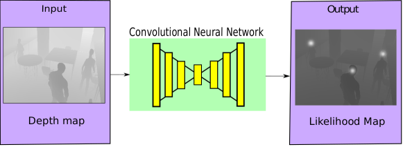
The non-overhead camera location is usually better than the overhead one in what respect to the greater amount of information it provides about the environment. In addition, it eliminates the need of using a specific camera pose, since many current surveillance systems cannot assume that restriction. PD3net receives a depth input map as input and produces two different outputs, see Figure 2. The CNN proposed here provides an output represented by a likelihood map that has the same size as the input image, i.e. it is spatially coincident. This output map shows the detections of people made by the system in pixel coordinates as we can see in the Figure 2.

Technically, the PD3net network core inherits the Resnet50 [27] internal blocks structure. This structure was also used by DPDnet but now it is meticulously revisited to fulfill the demanding real time requirements. At the neuron level, PD3net adds the Leaky ReLU activation function to the neuron, which clearly increment the speed of the gradient computation during the backpropagation and solves the dying ReLU problem, still remaining its non-linearity. At the layer level, PD3net introduces the spatially separable convolutions which considerably reduces the number of parameters and, consequently, the number of computations.

Finally, at structural level, a thorougly study of the number of layers was developed removing all layers whose detection improvements were negligible and slows down the people detection. Identity, deconvolutional and convolutional blocks were refined to minimize its number of parameters. Putting all these improvements together, PD3net achieves the sought real time with the best people detection rates, the most important contribution of the paper.

Figure 2: Depth input image and likelihood output map.

.

PD3net use the output format proposed by [19], in which we used a likelihood map with 2D Gaussian distributions in the center of the detected persons. This format allows using the center of the distributions as the 2D positions of the persons. In contrast to the overhead problem solved in [19], when moving to an elevated frontal position, the occlusions are one of the main problems that we have to face. The solution we propose to deal with them is the use of variable 2D Gaussian distributions which adapt themselves to avoid their overlap, allowing the system to become more robust against hard-occlusions.

The proposed method has certain pros and cons. In the case of the former, this system allows the detection of multiple people without ambiguity and in addition, the processing time is completely independent of the number of users detected. In the meantime, by contrast, firstly this system depends quite a lot on the hardware used, especially in terms of the quality of the 3D information obtained and secondly in terms of the positioning of the camera, since being a non-restrictive positioning requires the system to be much more general in its operation and to have a high level of independence from the camera pose.

3.2 Architecture of the PD3net Network

Here we proposed a new upgraded architecture, shown in Figure 3, for PD3net, where its basis its inherited from its predecessor [19].

Figure 3: System’s Architecture.

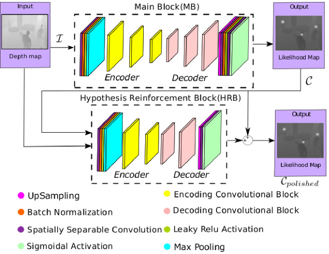
The base structure has similarities with the [19] architecture. It is composed of two important blocks that are the main block (MB) and the the hypothesis reinforcement block (HRB). These blocks are modeled by encoder-decoder architectures, which are traditionally used in tasks such as semantic segmentation [2, 48], 3D reconstruction, registration [16, 24], and deep fakes detection [25, 32].

The input depth image $\mathcal{I}$ with size $240\times 320$ is processed by the MB, which generates the first likelihood map $\mathcal{C}$ (also with size $240\times 320$), which is then concatenated with the input image $\mathcal{I}$, so that the input tensor of the HRB $\mathcal{I}_{2}$ is composed by the concatenation of $\mathcal{I}$ and $\mathcal{C}$, and has a size of $240\times 320\times 2$. The HRB polishes the initial likelihood map $\mathcal{C}$ and uses it as an output initialization, obtaining the final refined likelihood map $\mathcal{C}_{polished}$ ($240\times 320$), that validates, corrects and refines the predictions of the first map $\mathcal{C}$, thus improving its final results in $\mathcal{C}_{polished}$. The detailed structure of the MB can be seen in Table 2.

(a) Example comparison.

(b) General formulation

Figure 4: Differences between conventional and spatially separable convolutions.

Table 2: Detailed architecture of the main block.

Main Block (MB)
Layer	Output size	Parameters
Input	$240\times 320\times 1$	-
Convolution	$120\times 160\times 64$	kernel=(7, 7) / strides=(2, 2)
BN	-
Activation	Leaky ReLU
Max Pooling	$40\times 53\times 64$	size=(3, 3)
ECB	$40\times 53\times 256$	kernel=(3, 3) / strides=(1, 1) (a=64, b=64, c=256)
ECB	$20\times 27\times 512$	kernel=(3, 3) / strides=(2, 2) (a=128, b=128, c=512)
ECB	$10\times 14\times 1024$	kernel=(3, 3) / strides=(2, 2) (a=256, b=256, c=1024)
DCB	$10\times 14\times 256$	kernel=(3, 3) / strides=(1, 1) (a=1024, b=1024, c=256)
DCB	$20\times 28\times 128$	kernel=(3, 3) / strides=(2, 2) (a=512, b=512, c=128)
DCB	$40\times 56\times 64$	kernel=(3, 3) / strides=(2, 2) (a=256, b=256, c=64)
Cropping	$40\times 54\times 64$	cropping=[(0, 0) (1, 1)]
Up Sampling	$120\times 162\times 64$	size=(3, 3)
Convolution	$240\times 324\times 64$	kernel=(7, 7) / strides=(2, 2)
Cropping	$240\times 320\times 64$	cropping=[(0, 0) (2, 2)]
BN	-
Activation	Leaky ReLU
Convolution	$240\times 320\times 1$	kernel=(3, 3) / strides=(1, 1)
Activation	Sigmoidal
Output	$240\times 320\times 1$	-

The CNN proposed here introduces important modifications with respect to [19]. The most important change is the use of spatially separable convolutions instead of separable convolutions (depthwise convolution + pointWise convolution) [10]. The reason of this change lies in the fact that the separable convolutions isolate the depth channels in the phase of the depthwise convolution, and use the pointwise convolution to synthetically increase the depth of the output.

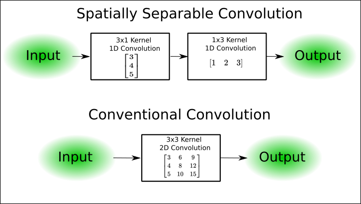
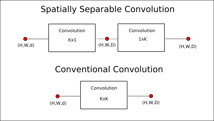
The operations performed by the separable convolutions can be harmful to the neural networks in some cases. The reason for this lies in the fact that especially the first layers of the convolutional neural network, where the characteristics of medium and low abstraction are found, in many cases complement each other. The break of these relationships or making them more complex by means of separable convolutional layers can eliminate important relationships between the features that reduce the model training capacity or efficiency. In order to solve this problem without the need to resort to separable convolutional layers, we have used spatially separable convolutional layers, such as those used by Inception V3 [54]. An example of Spatially Separable convolutions can be seen in Figure 4(a).

Spatially separable convolutions use two 1D filters to compose a 2D equivalent convolution, so that it forces the filters to be decomposable in two 1D filters. This allows reducing the number of operations and parameters under certain conditions, which are shown in equations 1, 2 and 3, where the variables $K$, $d$, $D$, $H$ and $W$ represent the kernel size, input depth of the tensor, final output depth of the tensor, height of the input tensor and width of the input tensor, respectively (as can be seen in Figure 4(b)).

The following equations shows the conditions necessary to accomplish to reduce the number of operations and parameters, additionally, these equations suppose a stride of $1$ and a constant size of the image compensated with the padding.

$$\begin{gathered}nparam_{conv}=KKdD=K^{2}dD\\ nops_{conv}=HWD(K^{2}d+(K^{2}-1)d)=HWD((2K^{2}-1)d)\end{gathered}$$ (1)

$$\begin{gathered}nparam_{sep}=KdD+KD^{2}\\ nops_{sep}=HWD(Kd+(K-1)d)+HWD(KD+(K-1)D)=\\ HWD((2K-1)(d+D)\end{gathered}$$ (2)

$$\begin{gathered}nparam_{conv}>nparam_{sep}\rightarrow K^{2}dD>KdD+KD^{2}\rightarrow\\ d>\frac{1}{(K-1)}D\\ nops_{conv}>nops_{sep}\rightarrow HWD((2K^{2}-1)d)>HWD((2K-1)(d+D))\\ d>\frac{(2K-1)}{2K(K-1)}D\end{gathered}$$ (3)

Once we have defined the conditions, we apply them to the three specific convolution cases used in the proposed CNN, where $K=3,5,7$. The obtained values are shown in table 3 where its last row shows the more restrictive condition that allows improving both the number of parameters and the number of operations.

Improvement in		$K=3$	$K=5$	$K=7$
Parameters	$d>\frac{1}{(K-1)}D$	$d>0.5D$	$d>0.25D$	$d>0.16D$
Operations	$d>\frac{(2K-1)}{2K(K-1)}D$	$d>0.416D$	$d>0.225D$	$d>0.154D$
Both		$d>0.5D$	$d>0.25D$	$d>0.16D$

Table 3: Conditions that the use of factorized convolutions must meet to be faster and more parameter efficient than conventional convolutions for the proposed CNN.

The main changes to the proposed architecture can be summarized as follows:

• Leaky Relu activation:We use Leaky Relu activations to improve the generalization and convergence, as we proposed in [62]. Leaky Relu helps to solve the ”dying relu” problem, where the zero activation zone of the Relu slows and destabilizes the training process. Instead of the zero activation zone, the Leaky Relu has a small negative slope that mitigates the problem.

• Spatially separable convolutions:In our proposal we use residual blocks with a certain basis of the ones used in [27], in terms of structure. The main difference is the inclusion of the spatially separable convolutions to speed up the network and solve the conventional separable convolution problems.

• Resized convolutions:In our proposal, we use the resized convolution as an approximation of the deconvolution process, with a nearest neighbor interpolation type. This is done to avoid the possible checkerboard artifacts that could appear in our output likelihood maps if we use the transposed convolution approximation, as discussed in [43]. Additionally, we prefer the nearest neighbor interpolation instead of bilinear or bicubic interpolation, because they led to problems in the interpolation of high-frequency image features, as explained in [43].

• Loss function: An important change with respect to [19] is that the loss function used in the proposed system is adapted to the problem of detecting people with the Gaussian modeling approach used, so that it seeks to give greater weight to the learning of those Gaussians against the learning of the background of the image, which favors the convergence of the system, which was strongly affected by this factor.

3.2.1 Architecture of the Main Block (MB)

The architecture of the Main Block (MB) is shown in Table 2, describing all its layers with its correspondent dimensions and parameters, where a, b and c are the numbers of filters of the internal layers in the Encoding Convolutional Blocks (ECBs), Decoding Convolutional Blocks (DCBs), and Identity Blocks (IBs).

The first layer of the MB uses the $240\times 320$ input depth image $\mathcal{I}$, and, through the residual blocks with spatially separable convolutions, it codifies and processes the input to finally deliver the first likelihood map $\mathcal{C}$. The encoder consists of IBs and ECBs, where the first ones process the input tensors with the same output size as the input block but with higher depth, while the second ones process the input and generates an output with half the input size and higher depth. As opposed to the encoder, the decoder consists of IBs and DCBs that increase the data size and decreases depth, to obtain an output with the same size as the input depth image $\mathcal{I}$.

Following the efficiency conditions previously defined for the spatially separable convolutions, these convolutions will only be included in the network elements suitable to be improved in complexity and speed.

Regarding the Main Block layers, we initially have an ordinary convolutional layer. This first layer is not spatially separable because it would not benefit from reduced complexity and increased speed, as introducing factorized convolution here would imply a computation time $10.24$ times slower than a conventional convolution. After the first convolution, a Batch Normalization and a Leaky Relu activation will be applied, to finally use a Max Pooling layer that will obtain the maximum energy of the filters.

After these initial filtering layers, we start to use the residual blocks, three ECBs and IBs will be used sequentially for the encoding process. They will be followed by another three DCBs and IBs that will be used sequentially for the decoding process. The final layers of the decoder use Cropping, ZeroPadding and UpSampling to accommodate the image size, to finally apply the last convolutional layer followed by a batch normalization and sigmoidal activation.

3.2.2 Architecture of the Hypothesis Reinforcement Block (HRB)

The Hypothesis Reinforcement Block (HRB) preserve the basic structure of [19], and it is a smaller version of the MB that uses residual blocks and spatially separable convolutions too. The HRB uses $\mathcal{I}_{2}$ as input, which is composed by $\mathcal{I}$ and $\mathcal{C}$ with a size of $240\times 320\times 2$ as explained above. In contrast to the proposal in [19] we have included an adder at the output that adds the output MB $\mathcal{C}$ to the HRB output and ensures that $\mathcal{C}$ is used as an initialization to the polishing process, as the HRB is in charge of obtaining the final polished likelihood map $\mathcal{C}_{polished}$. The HRB is composed firstly by the same structure as the MB, it uses a first convolutional layer, batch normalization, Leaky Relu activation, and max pooling. After that, the number of IBs, ECBs, and DCBs is reduced to two for each type. Finally the output layers follow a similar setup than the ones in the MB, with a final sigmoidal activation. Table 4 summarizes all the layers and blocks used in the HRB.

Table 4: Detailed architecture of the hypothesis reinforcement block.

Hypothesis Reinforcement Block (HRB)
Layer	Output size	Parameters
Input	$240\times 320\times 2$	-
Convolution	$120\times 160\times 64$	kernel=(7, 7) / strides=(2, 2)
BN	-
Activation	Leaky ReLU
Max Pooling	$40\times 53\times 64$	size=(3, 3)
ECB	$40\times 53\times 256$	kernel=(3, 3) / strides=(1, 1) (a=64, b=64, c=256)
ECB	$20\times 27\times 512$	kernel=(3, 3) / strides=(2, 2) (a=128, b=128, c=512)
DCB	$40\times 54\times 128$	kernel=(3, 3) / strides=(2, 2) (a=512, b=512, c=128)
DCB	$80\times 108\times 64$	kernel=(3, 3) / strides=(2, 2) (a=256, b=256, c=64)
Up Sampling	$240\times 324\times 64$	size=(3, 3)
Cropping	$240\times 320\times 64$	cropping=[(0, 0) (2, 2)]
Convolution	$240\times 320\times 64$	kernel=(3, 3) / strides=(1, 1)
BN	-
Activation	Leaky ReLU
Convolution	$240\times 320\times 1$	kernel=(3, 3) / strides=(1, 1)
Activation	Sigmoidal
Output	$240\times 320\times 1$	-

The ECBs and DCBs blocks are similar in structure. They are formed by two unbalanced links, where the first one has three convolutional layers, and the second has only one. The output of the blocks is composed of the added normalized output of the links. The main difference between the ECBs and DCBs lies in the convolutional process: the ECB uses a factorized convolution and the DCB uses a resized convolution. In the case of the IBs, they preserve the size of the input, so that one of the links only acts as a shortcut for the input to be directly added to the output of the three convolutional links. This preserves the input information and adds them to the output filtered information without changing the size. The architecture of the ECBs, IBs and DCBs is shown in Figure 5, where the parameters a, b and c are the layer depth or the number of filters in the corresponding layer. The number of filters of the third convolution in the bottom section must be equal to the number of filters in the top section (c parameter). The parameters a, b y c in Tables 2 and 4 and in Figure 5 have the same meaning.

Figure 5: Architecture of the ECBs, DCBs and IBs.

3.3 Training procedure

The network training process consists of two stages. In stage 1 we use a photorealistic synthetic database (created using the graphics simulator [5]) to train our CNN end to end. This allows the network to learn the most important features for the person detection task, while using a dataset that is automatically generated and labeled. In stage 2 we fine-tune the CNN to adjust its weights to the actual camera pose with a small real database, composed of only $3500$ frames that need to be manually labeled.

The use of the synthetic database allows us to avoid the need to use or create and label a large people detection database with depth images. The synthetic database has $22\cdot 10^{3}$ frames of depth images that simulate capturing from an elevated front position around a synthetic room.

In stage 1 we split the synthetic database in training and validation subsets composed by the 67% and the 33% percent of the database, respectively. The context used to create the synthetic database is a room similar to a laboratory with persons walking in different directions as we can see in the first two rows of Figure 6 as generated by Blender. In addition to this, we also changed the camera pose every frame, by rotating and moving it around the room. Our objective is changing the background in all the frames to prevent the CNN from learning a constant background. This approach allows the network to more easily generalize to different environments, as the CNN interprets the background as noise and focus in the people walking around, isolating the system from a given fixed perspective and pose of the camera.

Figure 6: Sample images of the Blender simulated room with different perspectives (top two rows), and samples of synthetic depth images for training (belonging to the GESDPD dataset, botom row).

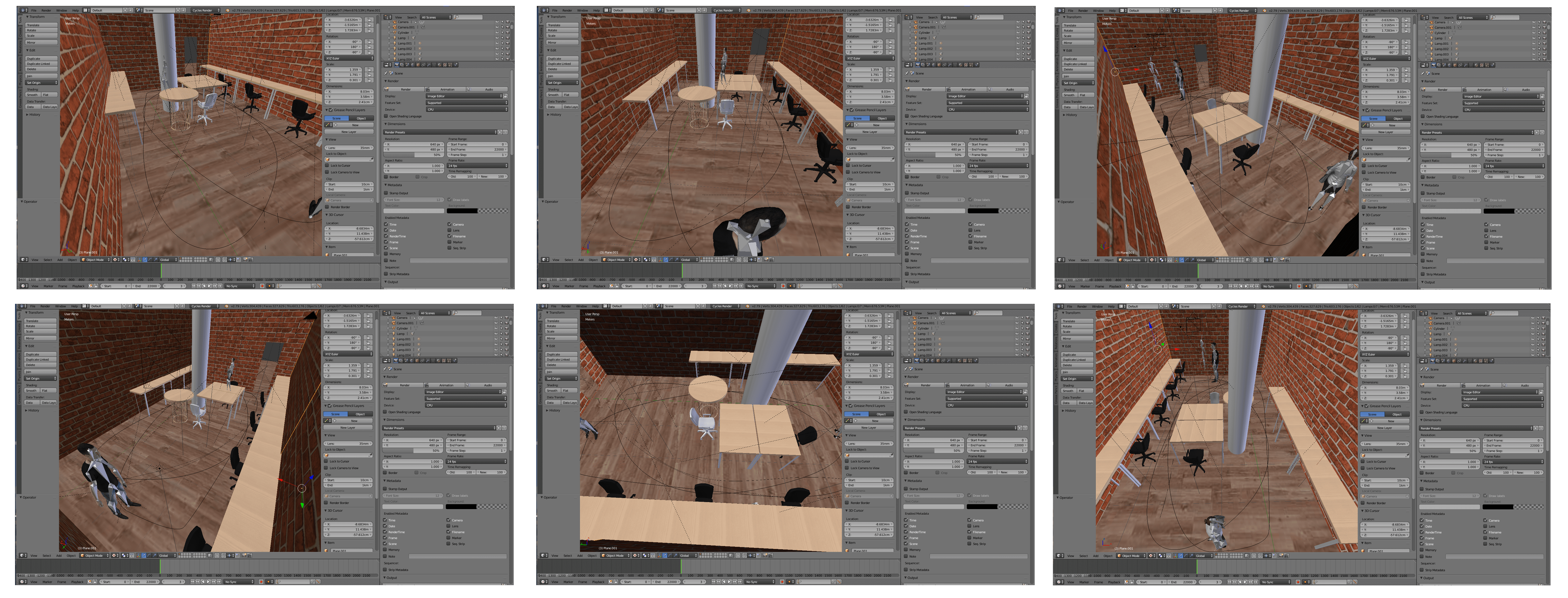
The images generated by the simulation software have a resolution of $240\times 320$, to be consistent with the images recorded with the camera in the real scenario. An example of the synthetically generated depth images can be seen in the bottom row of Figure 6.

In stage 2 we used a recorded and manually labeled real database composed by $3500$ frames recorded using a realsense D435 camera [29]. It was used fine-tune and adapt the network weights network to the real environment. This stage is necessary because the synthetic data do not consider problems that appears in a real scenario, such as motion blur, measurement noise or the influence of the ambient light in the depth measures.

Regarding the labeling process, and taking into account that the input image $\mathcal{I}$, the first likelihood map $\mathcal{C}$ and the polished likelihood map $\mathcal{C}_{polished}$ are normalized between $[0,1]$, we placed 2D Gaussian-like distributions in the centroid of the labeled people with a maximum value of 1 corresponding to the centroid. The standard deviation of the distributions is constant in all the cases because using variable gaussian deviation proved to decrease the detection performance in preliminary experiments. The gaussian deviation value has been calculated using the average estimate of a human head diameter, which is $\mathcal{D}=15$ pixels. Gaussian deviation is calculated as $\sigma=\mathcal{D}/2.5=15/2.5=6$.

One important modification on the labeling process as compared with the proposal in [19] is that the gaussians are not constant in terms of overlapping. Their standard deviations are constant, but when two gaussians overlap, we force a clear separation between them, as shown in Figure 7. This helps to mitigate the occlusions problem because there always exists a separation between gaussians, which in the post-processing will help to identify the people of the image. One example of how we handle the labeling in case of gaussian overlap can be seen in Figure 7.

Figure 7: Gaussians Overlap Example.

The optimization strategy we applied was Swats, proposed by [31]. It involves a first training phase with Adam [34] corresponding to stage 1, and a second phase with SGD+Momemtum that corresponds to stage 2. This strategy allows to improve the network generalization capabilities, as demonstrated in [31]. The initial learning rate of the first stage was $0.001$, which was combined with the use of an early stopping callback to save the best possible model. The adaptive skills of Adam modifies this learning rate along the training process. In the second stage we use the SGD+Momemtum learning rate equal to $1e-5$.

The loss function has also been strongly improved as compared with [19], in which the simple mean square error was used. Our CNN uses a training set composed of input depth images $\mathcal{I}_{i}$ and initial and polished likelihood maps $[\mathcal{C}_{i},\mathcal{C}^{polished}_{i}]$.

The proposed loss function tries to go beyond the conventional mean square error function using a customized weighting in the detection and background points, so that the system converges faster than in conventional function cases. The proposed loss function consists of 4 elements, which are differentiated by location and type of points to be evaluated. In the first case, we can separate in main’s block output location that its composed by the two first elements and the refinement output location that it’s composed of the third and fourth elements and have a superindex named as $polished$. In the latter case, the loss includes a weighting factor between the zero-negative value points marked by a $0$ symbol and the positive-non zero points of the likelihood map marked by a $+$ symbol. The first case helps to refine the likelihood maps provided by the main block while the second case improves the convergence to the gaussian distributions of the target likelihood map. The loss function is described in equation 4.

$$\begin{gathered}\mathcal{L}=\lambda_{1}\frac{1}{N}\sum_{i=1}^{N}\|\hat{\mathcal{C}_{i_{+}}}-\mathcal{C}_{i_{+}}\|^{2}+\lambda_{2}\frac{1}{N}\sum_{i=1}^{N}\|\hat{\mathcal{C}_{i_{0}}}-\mathcal{C}_{i_{0}}\|^{2}+\\ \lambda_{1}\frac{1}{N}\sum_{i=1}^{N}\|\hat{\mathcal{C}^{polished}_{i_{+}}}-\mathcal{C}^{polished}_{i_{+}}\|^{2}+\lambda_{2}\frac{1}{N}\sum_{i=1}^{N}\|\hat{\mathcal{C}^{polished}_{i_{0}}}-\mathcal{C}^{polished}_{i_{0}}\|^{2},\end{gathered}$$ (4)

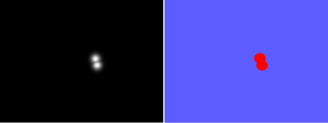
where $\lambda_{2}=1$ and $\lambda_{1}=1.3$ are the parameters that weight the importance of the zero-negative value points and the non-zero-positive points in the loss function. An example of the zero and non-zero points considered can be seen in Figure 8, where at the left side we have the original likelihood map and at the right in red we distinguish the non-zero points and in blue the zero points.

Figure 8: Example image of zero and non-zero points. In the left image, we can see an output likelihood map. Meanwhile in the right image we can observe the zero and positive-non-zero points plotted in blue and red respectively.

We trained the network for 30 epochs with the Adam Optimizer in the first stage, and for 20 epochs with SGD+Momemtum in the second stage, choosing the best possible model obtained along the training process.

4 Experimental Work

This section first describes the datasets (section 4.1) and the experimental setup (section 4.2). Then, we present the evaluated algorithms (section 4.2.1), and the used metrics (section 4.2.2). Finally, we provide details on the training and hyperparameter selection strategies (section 4.2.4) and the way to generate part of the metrics for the algorithm proposed here (section 4.2.3).

Once the experimental conditions and the data to be used are described, the results are presented through the use of tables and figures, in which the main metrics are detailed and a comparison between our proposal and other algorithms in the literature is carried out. The results are first presented for the synthetic data case (section  4.3) which allows us to introduce and explain in-depth the effectiveness of a synthetic pre-training as the one performed here, and which are the limitations that can be found in the real world. After explaining the synthetic training, the real results are presented in each of the databases used (section  4.4). This explanation ends with a comparison of the average results of all the databases (section 4.4.6) and a discussion about the use of a global training approach to the system (section 4.4.7). After the presentation of the results, the computational performance is then evaluated quantitatively (section 4.5).

4.1 Datasets & Data Partition

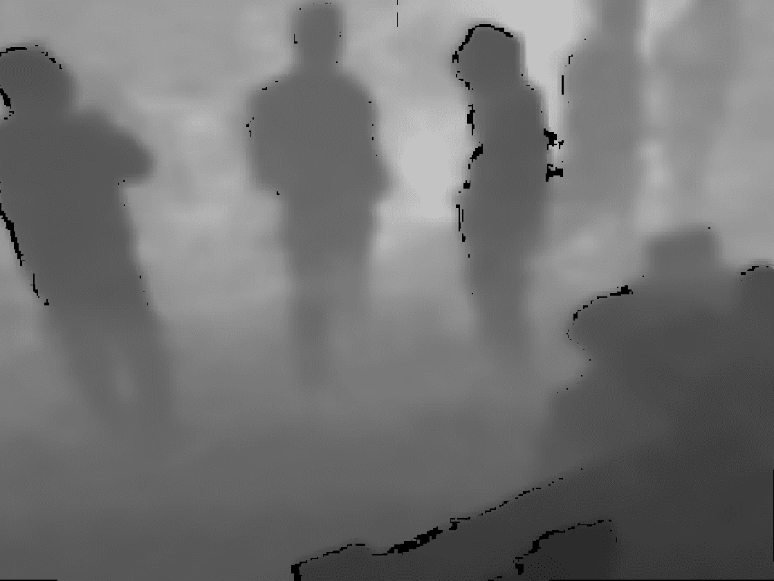
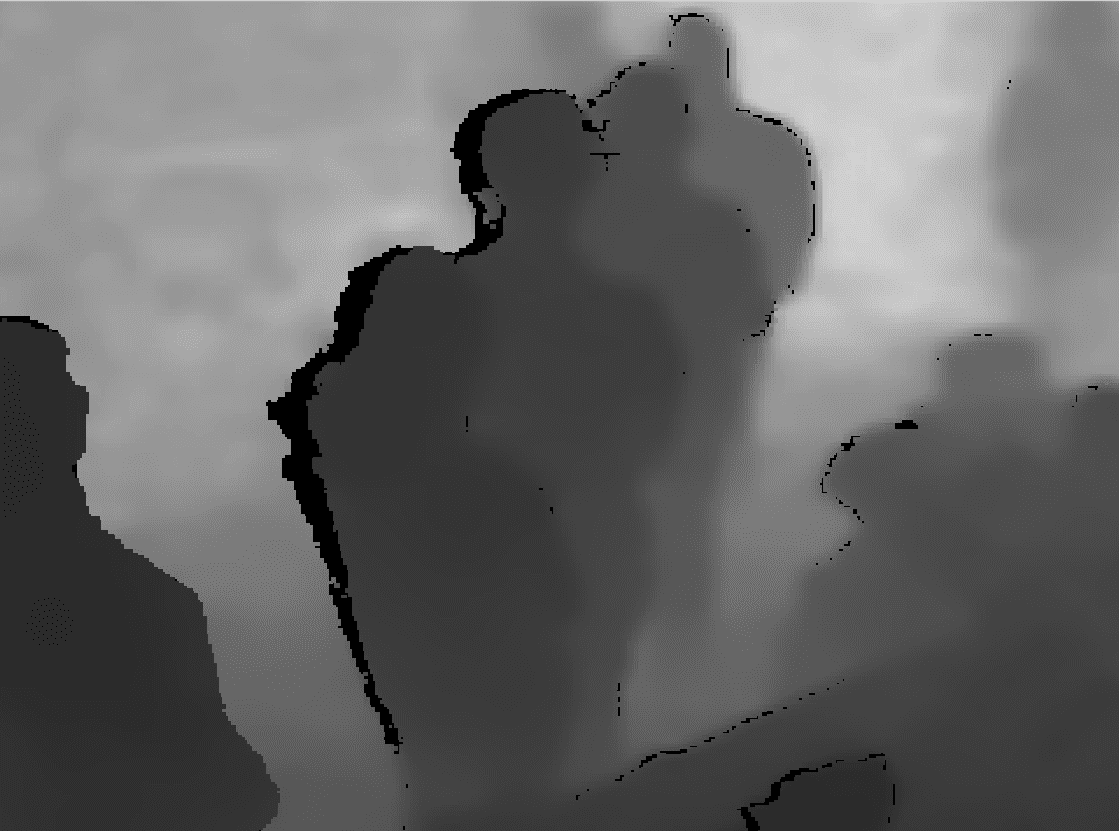
In order to provide a wide range of evaluation conditions, we have used five different databases, that will be described next. Figures 9 and 10 provide some sample frames to give an idea on the style and quality of the different datasets.

1. GESDPD [18]: GESDPD is a synthetic dataset which contains 22000 depth images, that simulate to have been taken with a sensor in an elevated front position, in an indoor working environment. These images have been generated using the simulation software Blender [5]. The simulated scene shows a room with different people walking in different directions. The camera perspective is not stationary, as it rotates and moves along the dataset, which avoids a constant background that could be learned by CNN in the training, as can be seen in figure 6, that shows different perspectives of the synthetic room in the simulation software Blender [5]. Using different backgrounds around the synthetic room allows CNN to see the background as noise and focus the training in the people that come along the image, immunizing the network to the change of camera perspective and assembly conditions.

   The generated images have a resolution of $320\times 240$ pixels codified as 16 bits unsigned integers. Some examples of the synthetic images are shown in figure 6, the images correspond to three different perspectives, and the depth values are represented using a colormap.

2. GFPD [17]: The Geintra Frontal Person Detection dataset is a high-resolution dataset recorded with a [29] realsense D435 camera. GFPD contains 5270 depth frames with 13827 annotated people instances. The camera has an active stereo depth sensor that provides depth maps with a resolution of $1280\times 720$. The records of this dataset consider a great variety of conditions including different sensor heights (2200-2700 mm), different tilt angles (26-41 degrees), as well as different backgrounds and lighting conditions.

3. EPFL [3], that includes two different datasets:

   1. EPFL-LAB: The first one (EPFL-LAB) contains around 1000 RGB-D frames with around 3000 annotated people instances. There are at most 4 people who are mostly facing the camera, presumably a scenario for which the Kinect software was fine-tuned.

   2. EPF-CORRIDOR: The second one (EPFL-CORRIDOR) was recorded in a more realistic environment, a corridor in a university building. It contains over 3000 frames with up to 8 individuals, and it is a challenging dataset since there are important occlusions.

4. KTP [42]: The Kinect Tracking Precision dataset (KTP) presented in [42] contains several sequences of at most 5 people walking in a small lab environment. They were recorded by a depth camera mounted on a robot platform and we use here the only one that was filmed while the camera was static. Authors provide ground truth locations of the individuals both on the image plane, and on the ground plane. Unfortunately, the quality of the ground truth for the ground plane is limited, due to the poor quality registration of the depth sensor location to the environment. In order to fix this, we made an effort and manually specified points corresponding to individuals on the depth maps, then projected them on the ground plane, and took an average to get a single point representing person location. This introduces a small bias as we only observe the outer surface of the person but any motion capture system would have similar issues.

5. UNIHALL [51]: In [51, 39], the authors report their results in a dataset containing about 4500 RGB-D images recorded in a university hall from three statically mounted Kinect cameras. Unfortunately, there is no ground plane ground truth available, thus we only report results for image plane. To compare to their results, we follow the evaluation procedure described in [51], that is, without penalizing approaches for not detecting occluded or hidden people. We also report our performance for the full dataset separately.

(a) Sample frames from the GESDPD dataset [18].

(b) Sample frames from the GFPD dataset [17].

(c) Sample frames from the KTP dataset [42].

Figure 9: Sample frames from the GESDPD, GFPD and KTP databases (gray coded depth).

(a) Sample frames from the EPFL-LAB dataset [3].

(b) Sample frames from the EPFL-CORRIDOR dataset [3].

(c) Sample frames from the UNIHALL dataset [51].

Figure 10: Sample frames from the EPFL-LAB, EPFL-CORRIDOR and UNIHALL databases (gray coded depth).

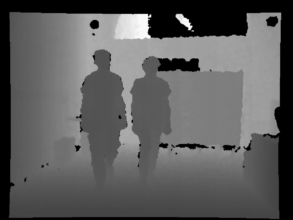
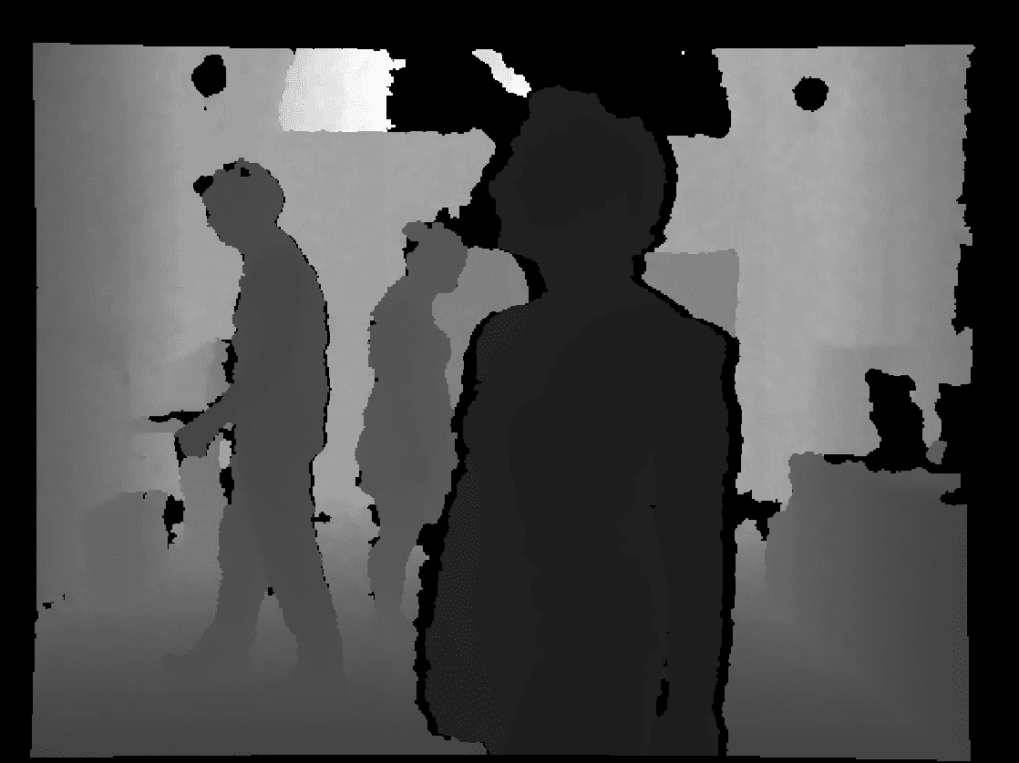
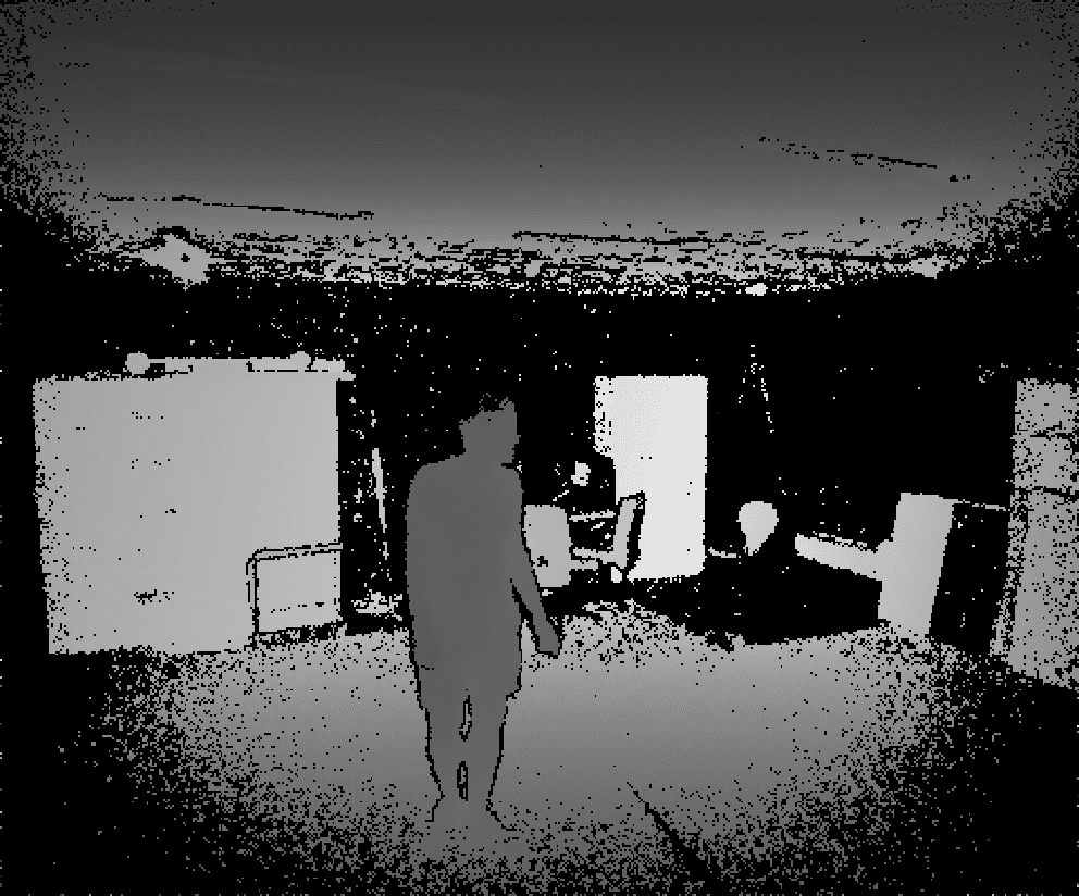
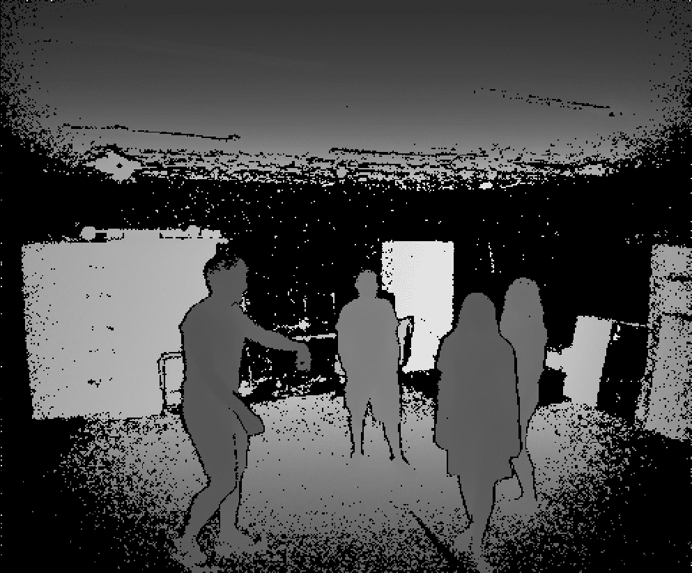
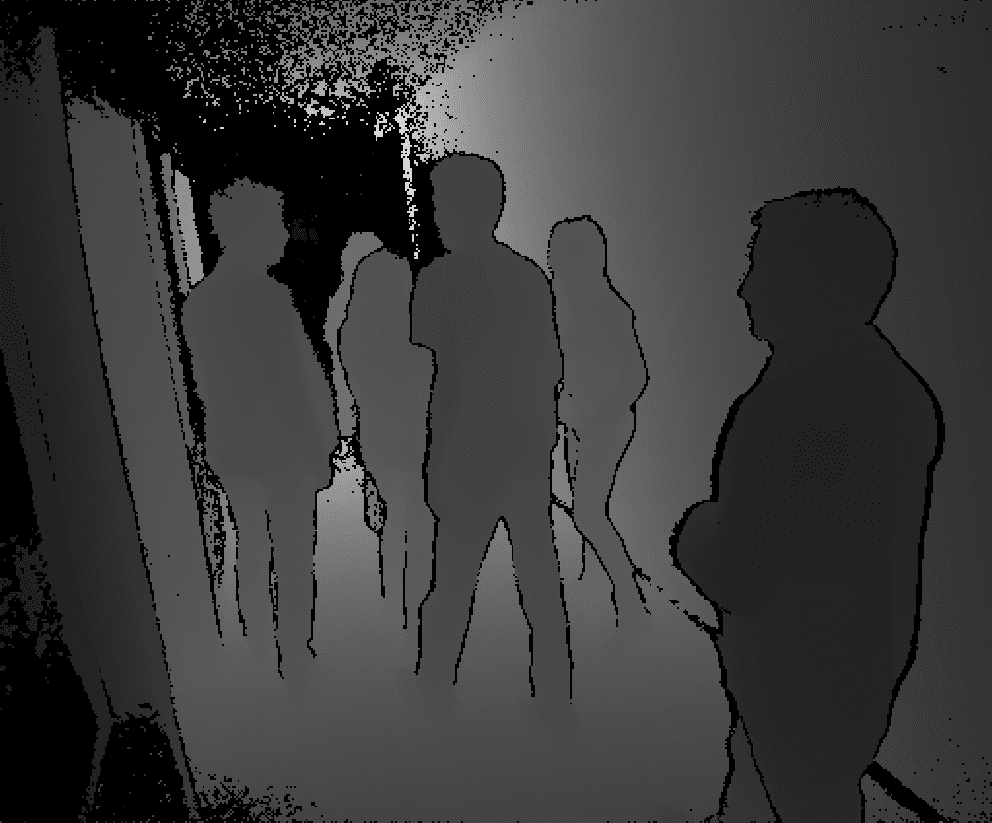
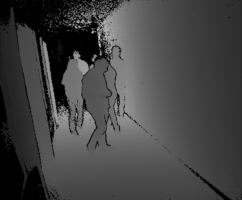
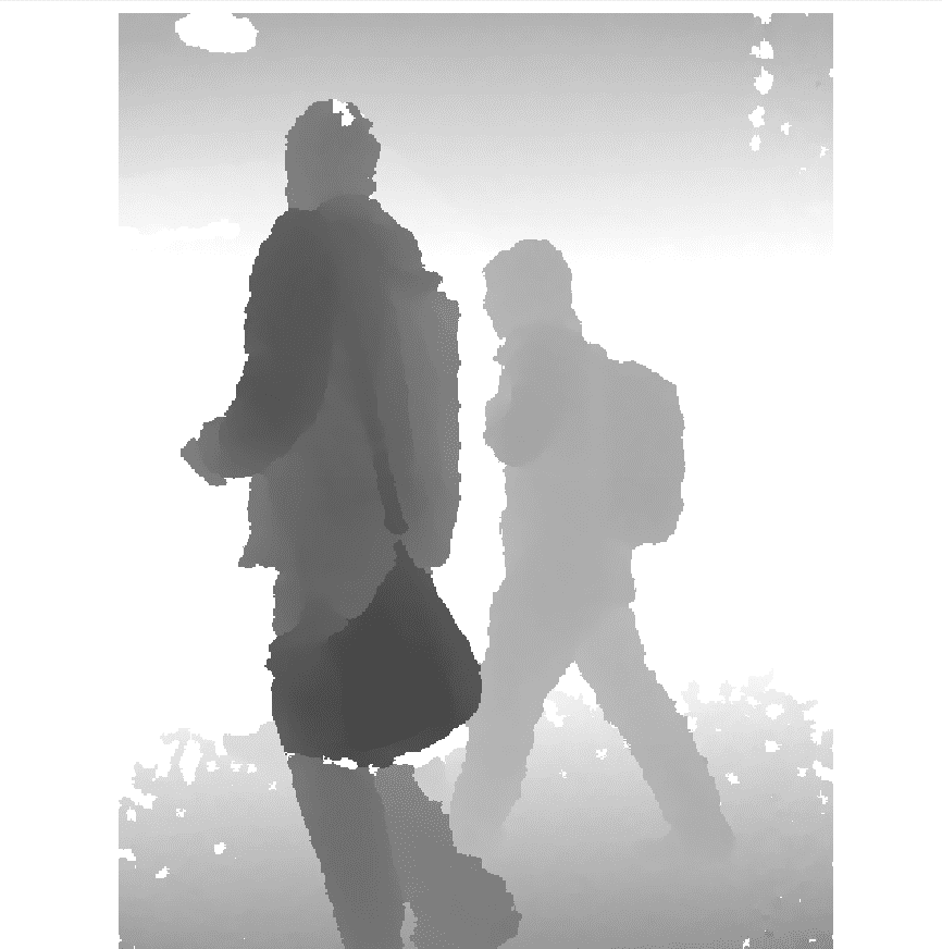
In what respect to the data partitioning we did to generate the training and testing subsets, Table 5 shows the total number of frames (column #framesFull), the total number of people labeled in the ground truth in these frames (column #PeopleFull), and the partition statistics for the training subsets (columns #framesTrain and #PeopleTrain), and for the testing subsets (columns #PeopleTest and #framesTest). It also provides details, wherever necessary, on the sequences used. Total numbers are shown right-aligned, and when the partition involved several sequences, the corresponding data for individual sequences is shown left-aligned. To give an idea on the relative size of the training and testing material for each dataset, Table 5 also provides the percentages corresponding to these subsets in the rows with accumulated totals for the #PeopleTrain and #PeopleTest columns.

Table 5: Data partition details.

	Sequence	#framesFull	#PeopleFull	#FramesTrain	#PeopleTrain	#FramesTest	#PeopleTest
GESDPD		22000	54215	17600	36063	4400	18152
					(67%)		(33%)
GFPD	1	1690	4462	1690	4462
	2	900	3760	900	3760
	3	1090	4337			1090	4337
	4	500	1268	500	1268
	Total GFPD	4180	13827	3090	9490	1090	4337
					(69%)		(31%)
EPFL-LAB	1	920	2287	600	1385	320	902
					(61%)		(39%)
EPFL-CORRIDOR	20141008_141829_00	390	899	390	899
	20141008_1414_30_00	420	813	420	813
	20141008_141913_00	396	1886	396	1886
	20141008_141537_00	430	853			430	853
	20141008_141537_00	1100	3581			1100	3581
	Total EPFL-CORRIDOR	2736	8032	1206	3598	1530	4434
					(45%)		(55%)
KTP	ROTATION	2200	3299	2200	3299
	STILL	2100	3420			2100	3420
	Total KTP	4300	6719	2200	3299	2100	3420
					(49%)		(51%)
UNIHALL	mensa_seq0_1.1	2900	2979	1400	2054	1500	925
					(69%)		(31%)
ALL Datasets	Total ALL Datasets	37036	88059	26096	55889	10940	32170
					(63%)		(37%)

4.2 Experimental setup

4.2.1 Evaluated algorithms

We compared the performance of our proposal PD3net with up to ten different strategies described in the literature that use depth cameras with an elevated non-overhead position in a people detection task.

Table 6 shows the main characteristics of all the evaluated methods, considering both classical and DNN approaches. It is relevant to note that we are comparing our depth-only proposal with others using different combinations of RGB and depth information, which imposes strong differences in the quality of the exploited data.

Table 6: Evaluated state-of-the-art methods for multiple people detection.

Solutions	Methods	Input information	References
[HTML]FFFFFF	ACF	RGB	[13]
[HTML]FFFFFF	PCL-Munaro	RGB-D	[42]
[HTML]FFFFFF	Kinect2	RGB-D	[33]
[HTML]FFFFFFClassic	Unihall	RGB-D	[51]
[HTML]FFFFFF	DPOM	D	[3]
[HTML]FFFFFF	RCNN	RGB	[23]
[HTML]FFFFFF	RGBCNN	RGB	[69]
[HTML]FFFFFF	RGBCECDCNN	RGB-D	[69]
[HTML]FFFFFFDNN	YOLO V3	RGB	[46]

Below, we explain in detail the evaluated state-of-the-art methods we use in the comparison:

• ACF [13]: That uses a RGB detector from [13], based on AdaBoost and aggregate channel features [14] to give a sense of what a state-of-the-art detector that does not use depth can do on these sequences.

• PCL-MUNARO [42]: That uses a RGB-D detector from [42], based on modified HOG features on regions extracted by depth segmentation.

• KINECT2 [33]: Based on the results obtained from the human pose estimation of the latest Kinect for Windows SDK [33]. It is not publicly known what specific algorithm is used. However in [50], the authors report that their algorithm is at the core of the human pose estimation for the older version of the Kinect software. For undisclosed reasons, the framework supports tracking up to 6 people, with the working depth range limited to 4.5 meters. To ensure fairness, we kept these restrictions in mind when using the EPFL-LAB and EPFL-CORRIDOR datasets. We do not penalize algorithms for not detecting more than 6 people or people who are further than 4.5 meters away.

• UNIHALL [51]: That uses a RGB-D detector from [51] based on HOG and HOD features. The code is not available and we, therefore, report only a single point on the precision-recall curve.

• DPOM [3]: This method checks for a human presence on the ground plane using bayesian inference. Before that, the first step is to detect the ground plane and remove it from the 3D processed point cloud. After the ground plane elimination, all the points that remain will be clustered and segmented as possible person detections. The algorithm stops when it finishes to group all the regions clustered in the whole depth image.

• RCNN [23]: That uses a region proposal based CNN with the [23] architecture. This architecture was originally used for region segmentation and classification. In addition to this architecture, it uses the region of interest method from [69].

• RGBCNN [69]: That uses a RGB CNN-based object detector with region of interest selection based on [69] and selective search from [56].

• RGBCECDCNN [69]: That uses a RGB and Depth combined CNN-based object detector with CECD channel encoding based on [69] proposal.

In addition to these methods, and to allow for additional experimentation on our GESDPD dataset, we have also used the YOLO (You Only Look Once) object detector [46] to be applied in the person detection task using depth and RGB data. Our use of the YOLO strategy comprises two approaches, using the YOLO system as is, and adapting it to more properly handle the depth information. These are the two developed systems on this line:

• YOLO-V3 [46]: RGB object detector [46] based on CNN and bounding box based approximation. This implementation was based on the original Yolo V3 architecture and trained with the COCO 2017 dataset [37]. The parameters used to configure the architecture were an input image size of $416\times 416$, 9 anchors, and all the COCO classes.

• YOLO-Depth: Depth object detector based on the [46] structure, but modified and retrained to only use depth information. This implementation was based on a modified Yolo V3 architecture to use depth images as input instead of RGB images. This implementation is trained with the depth datasets used in this paper. The parameters used to configure the architecture, were an input image size of 416x416, 9 anchors, and only with the person class. No structural changes have been made to the architecture as compared to the original version.

4.2.2 Evaluation Metrics

To provide a detailed view of the performance on the evaluated algorithms, we have calculated the main standard metrics in a detection problem, namely $Precision{}$, $Recall{}$, and $F_{1score}{}$. The results are shown both in tables (to provide the precise values), and in bar graphs (to provide an easier visual comparison).

In the scoring process, the following convention has been adopted regarding occlusions: In the case that an occluded person is not detected, it does not generate a detection error if the heads of the users are occluded in a percentage higher than 50%. Therefore the occlusion limitation does not practically affect occlusions between the bodies of the users, but only considering the occlusion of the upper body part.

In the results tables, we also include confidence intervals for the $F_{1score}{}$ metric, for a confidence value of $95\%$, to assess the statistical significance of the results when comparing different strategies. Additionally, the confidence intervals for the $Precision{}$, $Recall{}$, and $F_{1score}{}$ metrics are also shown in the bar graphs.

In the evaluation with real data, $Precision{}$-$Recall{}$ curves are also included. In the case of the DPOM, ACF, KINECT2, UNIHALL, PCL-MUNARO, RGBCNN, and RGBCECDCNN algorithms, we use those already provided in [69] and [3]. For the YOLO-Depth and YOLO-V3 [46] algorithms, we generate the curves of $Precision{}$-$Recall{}$ through a sweep of the algorithm confidence threshold. However, building these curves in our proposal is somehow artificial, leading to curves with strange appearances, as the threshold sweep is done on the Gaussian distribution threshold. In Section 4.2.3 we describe the $Precision{}$-$Recall{}$ curve generation procedure for our proposal, and the considerations that should be taken into account when addressing the interpretation of the $Precision{}$-$Recall{}$ curves for our system.

In the case of the $F_{1score}{}$, the obtained curves are scanned with each of the possible thresholds, to obtain their corresponding $F_{1score}{}$ and to be able to create the $F_{1score}{}$ vs threshold curve, which allows choosing the best point or range of points of the work following the criterion of the best possible $F_{1score}{}$.

An additional parameter of the evaluation metrics is the region on which they are calculated, including restrictions on the image plane and the depth range. In some cases (that will be clearly stated when showing the results), the evaluation metrics have been calculated considering:

• An image plane region which is smaller than the full-frame size. The objective is to only focus on full detections of people, avoiding the cases of incomplete persons in which they could otherwise be partially occluded by the image borders.

• A depth range that is smaller than the full depth range of the sensor. The objective is avoiding measurements greatly contaminated with noise that, for some recording conditions, can be found near the image borders or at depths near the sensor sensing limits.

4.2.3 $Precision{}$-$Recall{}$ curves generation for the PD3net algorithm

In this section we provide details on how the threshold to be optimised in PD3net works. The need for this explanation is given because it is not a conventional confidence threshold like the one that can be found in algorithms such as YoloV3 (in which the threshold sweep generates a smooth variation in the performance curves), so that it can produce effects that are radically different from the usual ones, which can be reflected in the $Precision{}$-$Recall{}$ curves.

Figure 11 shows a schematic example of a gaussian-like confidence map, which could be generated by our system. In the 2D representation of the figure (left image), we can see two small gaussian-like regions with a small overlap between them. In the three-dimensional representation (right image) the apparent overlap between the two gaussian structures is greater than the one observed in 3D.

Figure 11: Schematic representation of the 2D confidence map in 3D.

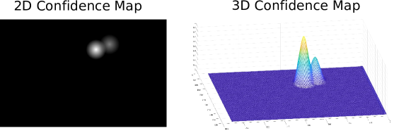
The threshold defined in the PD3net algorithm would be shown geometrically as a plane parallel to the XY plane that would cut the Gaussian distributions at a particular height, separating them both by their maximum height and by their overlap at the threshold level. So unlike conventional thresholds, this threshold will model both the intergaussian overlap and the maximum confidence peak.

Figure 12 shows the three-dimensional representation of the two detected gaussians after the application of three thresholds values at $0.1$, $0.4$, and $0.8$.

Figure 12: Representation of the effect of different threshold values.

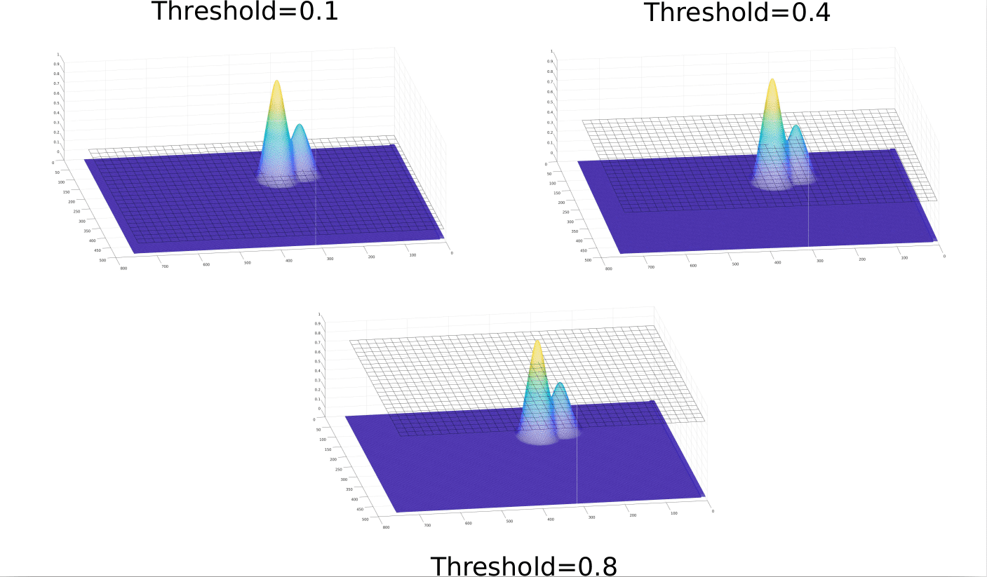
In the case of the $0.1$ threshold, it can be seen that the two gaussians are overlapping by their intersection at the threshold level, so that in terms of detections, it would generate a single detected person. In the case of the $0.4$ threshold, it can be observed that the gaussians no longer have overlap considering the threshold level, so that the two gaussian centroids are correctly detected. Finally, in the case of the $0.8$ threshold, only the gaussian with the highest height would found, since the other one is below the detection threshold, and would be discarded.

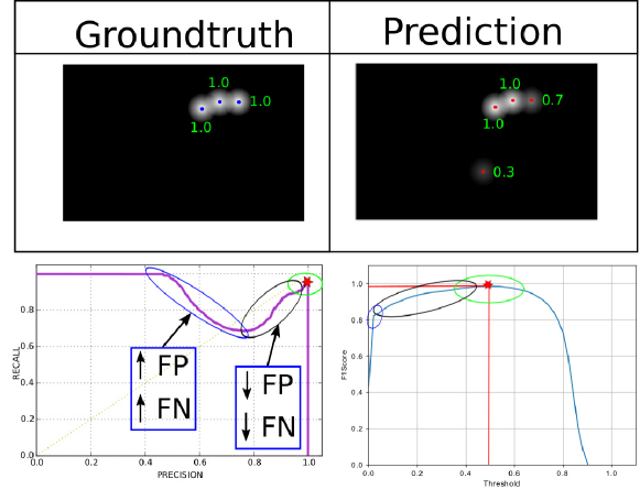
To show a real example on how we build the $Precision{}$-$Recall{}$ curves for the PD3net system, Figure 13 includes data obtained for a sample frame of the GFPD dataset. The upper part of the figure includes the ground truth confidence map (left image), showing three users with gaussians normalized at their maximum peaks of $1.0$, and the network prediction (right image), with four estimated gaussians whose maximum peaks correspond to $1.0$, $0.7$ and $0.3$ (not all the predictions will reach the $1.0$ level).

In the lower part of Figure 13 we can see two graphs. The one to the left is the $Precision{}$-$Recall{}$ graph on the test set, and the one to the right is the $F_{1score}{}-Threshold$ graph calculated on the training set. In these two graphs we find three well-differentiated sections that will allow to get an idea of the distribution of $Precision{}$-$Recall{}$ curve values when varying the threshold value:

• The first region, indicated by a blue ellipse, covers a threshold range below $0.1$. In that range, due to the increased gaussian overlapping and the acceptance of low confidence gaussians, the number of false positives and false negatives increase.

• The second region, indicated by a black ellipse, covers a wide threshold range below $0.1$ and $0.4$. In that range, as we increase the threshold value the gaussian overlapping will decrease, and also the gaussians with low confidence values will be discarded, thus decreasing the number of false positives and false negatives.

• The third region, indicated by a green ellipse, covers a wide threshold range between $0.4$ and $0.8$, and is where the system performs the best, with well and correctly separated gaussians, and good rejection of low confidence ones. This behaviour leads to the optimum working point shown as a red star.

Figure 13: Representation of the threshold variation effect on a GFPD example. From this example, we can conclude that a threshold variation will have a simultaneous impact on both the false positive rate (all the low confidence gaussians for low threshold levels) and the false negatives (all the overlapping gaussians for low threshold levels).

4.2.4 Training and threshold selection strategy

As discussed above, one of the key issues in the PD3net proposal is the correct selection of the detection threshold used in the output map $C_{polished}$. This selection is an important point because this threshold is responsible for deciding which gaussians distributions will be considered as possible person detections. The network and threshold training have been done using two different approaches:

• Tuned (Dataset specific) network training and threshold selection: In this scenario, the network has been trained on the training subset for each specific dataset, and the corresponding threshold is selected as that achieving the best $F_{1score}{}$ on this training subset. This way we can evaluate the best possible result with the threshold tuned to the conditions of each particular dataset.

• Global network training and threshold selection: In this secenario, the network has been trained on all the available training subsets, and the threshold has been selected as that achieving the best $F_{1score}{}$ on these training subsets. This way we can evaluate a realistic performance using the same single threshold for all the datasets.

4.3 Results training with Synthetic Data Only

Our first evaluation task was devoted to the evaluation of till what extent the training with simulated data could cope with the variability found in real datasets. To do so, we first run a set of preliminary experiments using the GESDPD as the training data, and both, GESDPD and EPFL-Lab for testing.

The first row in Table 7 shows the results of our proposal trained with the GESDPD when evaluated on an independent subset of the GESDPD dataset. The results indicate that the simulated training data seems to be valid to achieve reasonably good results when facing similar simulated conditions, with an overall error below $6.8\%$ and an $F_{1score}{}$ of $96.5\%$.

Table 7: Results on the GESDPD and EPFL-LAB datasets, trained on the training subset of the GESDPD.

	#FramesTest	#PeopleTest	$FN$ ($FNR\%$)	$FP$ ($FPR\%$)	$Error$	$Precision$	$Recall$	$F_{1score}$
GESDPD	$2200$	$3176$	$212$ ($6.68\%$)	$3$ ($0.09\%$)	$6.77\%$	$99.89\%$	$93.32\%$	$96.50\pm 0.11\%$
EPFL-LAB	$950$	$1959$	$474$ ($24.07\%$)	$3$ ($0.15\%$)	$24.35\%$	$99.80\%$	$75.80\%$	$86.16\pm 1.53\%$

The second row of Table 7 shows the results of our proposal trained with the GESDPD and evaluated on a testing subset of the EPFL-LAB dataset. In this case, the search area in the image plane was restricted to $280\times 150$ and the depth range considered up to $3.5m$. Our objective was to produce an environment more controlled in which unnecessary noise is removed from the image, present for example in the ceiling which occupies 40%of the image or on the floor. These results indicate that the simulated training data is not capable of leading to reliable results when facing a realistic dataset, with an overall error above $24\%$ and an $F_{1score}{}$ of $86.16\%$.

These preliminary experiments clearly indicate that training with simulated data only is still far from allowing us to get good results on realistic data. This conclusion leads us to develop a training procedure in two stages: first a full training using the simulated data, and then use a small subset of each of the evaluated datasets to fine-tune the pre-trained model.

4.4 Results on real data

In this section, we present the results and discussion when evaluating our proposal on the realistic datasets described in Section 4.1, and using all the available algorithms in each case. Table 8 shows the results of all the evaluated algorithms in all the available datasets. Empty cells in the table are due to the fact that the corresponding algorithms were not available, so that we have replicated the results published by the respective authors in the given datasets.

Table 8: Performance results on all the avaible datasets comparing the“tuned” and “global” versions for the PD3net proposal ($P=Precision,R=Recall{}$ (best result are displayed with green background, and orange background indicates results within the best one significant bands).

	GFPD			KTP			UNIHALL			EPFL-LAB			EPFL-CORRIDOR
	$P{}$	$R{}$	$F_{1score}{}$	$P{}$	$R{}$	$F_{1score}{}$	$P{}$	$R{}$	$F_{1score}{}$	$P{}$	$R{}$	$F_{1score}{}$	$P{}$	$R{}$	$F_{1score}{}$
PD3net tuned	$99.7$	222$96.36$	222$98.0\pm 0.20$	$96.2$	$96.3$	$96.3\pm 0.64$	222$92.5$	222$99.2$	222$95.7\pm 1.30$	white$98.8$	222$94.5$	222$96.6\pm 1.18$	$90.3$	222$80.1$	222$84.9\pm 1.05$
PD3net global	222$100.0$	white$95.9$	orange$97.9\pm 0.21$	$95.4$	$95.1$	$95.3\pm 0.71$	$91.2$	$97.3$	orange$94.2\pm 1.51$	$99.5$	$92.5$	orange$95.9\pm 1.30$	$90.9$	$76.1$	orange$82.8\pm 1.11$
YOLO-V3	$82.3$	$86.4$	$84.3\pm 0.53$	222$99.1$	222$98.2$	222$98.7\pm 0.39$	$84.5$	$93.1$	$88.6\pm 2.05$	$93.3$	$93.0$	$93.2\pm 1.65$	$58.6$	$59.8$	$59.2\pm 1.45$
YOLO-Depth	$79.8$	$55.1$	$65.2\pm 0.69$	$91.1$	$72.3$	$80.6\pm 1.32$	$63.2$	$52.4$	$57.3\pm 3.19$	$90.2$	$89.2$	$89.7\pm 1.98$	$78.4$	$47.9$	$59.5\pm 1.45$
PCL-MUNARO				$98.7$	$76.4$	$86.1\pm 1.16$	$82.5$	$78.2$	$80.3\pm 2.56$	$96.9$	$86.5$	$91.4\pm 1.83$	$95.0$	$56.3$	$70.7\pm 1.34$
DPOM				$95.3$	$94.5$	$94.9\pm 0.74$	$90.2$	$98.1$	orange$94.0\pm 1.53$	$98.5$	$85.4$	$91.5\pm 1.82$	222$96.3$	$70.9$	$81.7\pm 1.14$
ACF				$87.4$	$72.7$	$79.4\pm 1.36$	$90.2$	$85.4$	$87.7\pm 2.11$	$83.8$	$86.4$	$85.1\pm 2.33$	$66.3$	$40.3$	$50.1\pm 1.47$
RCNN							$50.1$	$51.4$	$50.7\pm 3.22$
RGBCNN							$49.7$	$51.2$	$50.4\pm 3.22$
RGBCECDCNN							$52.3$	$52.3$	$52.3\pm 3.22$
UNIHALL							$86.3$	$84.5$	$85.4\pm 2.28$
KINECT2										222$99.8$	$38.2$	$55.3\pm 3.24$	$86.3$	$41.2$	$55.8\pm 1.46$

For the PD3net algorithm, two results are provided for the conditions discussed in Section 4.2.4: one with the tuned version of the network model and threshold, and the other with their globally trained versions. The results show, as expected, a slight decrease in performance when using the global threshold as compared to the tuned one, but these differences are not statistically significant. This support the conclusion that the PD3net strategy is robust enough to face very different training and testing conditions.

In the next subsections we discuss the results for each specific dataset, providing a graphical comparison of the evaluated metrics, along with the $Precision{}$-$Recall{}$ and $F_{1score}{}-threshold$ curves for the tuned approach. The discussion of these curves for the global approach is later addressed in Section 4.4.7.

4.4.1 Results for the GFPD database

The second column of Table 8 and Figure 14 show the results when evaluating on the GFPD dataset, using our proposal PD3net and the YOLO-V3 and YOLO-Depth algorithms. We could not apply any of the other proposals described in Section 4.2 as they were not readily available.

Figure 14: Results on the GFPD dataset.

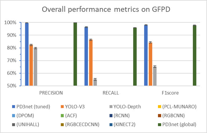
The results in the table show that both approaches of the PD3net algorithm clearly outperform the YOLO-based strategies, being the best in the three metrics used and in a statistically significant way, placing a great distance between it and YOLO-V3 as the second-best solution. The worse results of the YOLO-based algorithms probably rely in the fact that they were not designed to deal with depth data, and to the great number of occlusions and complex situations that GFPD contains.

Figure 15 shows the $Precision{}$-$Recall{}$ curve corresponding to the behavior of the three algorithms and the $F_{1score}{}-threshold$ curve corresponding to the PD3net algorithm. As described in Section 4.2.3, the appearance of the curve for our proposal is far from standard, and it is due to the effect of the threshold sweep procedure so that the area under the curve should not be taken into account as the comparison metric, but the actual working point of the algorithm (marked with a red start). The figure clearly shows that our working point greatly outperforms the other proposals.

Figure 15: $Precision{}$-$Recall{}$ curve comparison and $F_{1score}{}$-Threshold results for the experiments on the GFPD dataset.

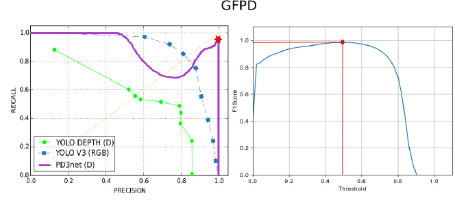
With respect to this $Precision{}$-$Recall{}$ curve, $F_{1score}{}$ metric is represented as a function of the threshold sweep used to generate the $Precision{}$-$Recall{}$ curve. This curve shows how the working point is located in the middle of a reasonably wide and flat area which outperforms the other two algorithms, indicating that its sensitivity to the threshold value is reduced.

The capabilities of our proposal are further established in the next sections where the availability of performance metrics on additional datasets and with a broad range of different algorithms are exploited in the comparisons.

4.4.2 Results for the KTP database

The third column of Table 8 and Figure 16 show the results when evaluating on the KTP dataset, using our proposal PD3net, the YOLO-V3 and YOLO-Depth algorithms, and three other proposals from the literature (DPOM, ACF and PCL-MUNARO).

From the table, it is surprising the top performance of the YOLO-V3 algorithm in terms of $F_{1score}{}$, with statistically significant different as compared with the second-best result (achieved by our PD3net). In this case, the YOLO-V3 system obtains better results than all the other proposals as the KTP database does not contain a lot of hard occlusions and has been prepared from a low frontal perspective, which are the perfect conditions for the operation of YOLO-V3, whose training images are also low frontal and with almost no occlusions.

Figure 16: Results on the KTP dataset.

Figure 17: $Precision{}$-$Recall{}$ curve comparison and $F_{1score}{}$-Threshold results for the experiments on the KTP dataset.

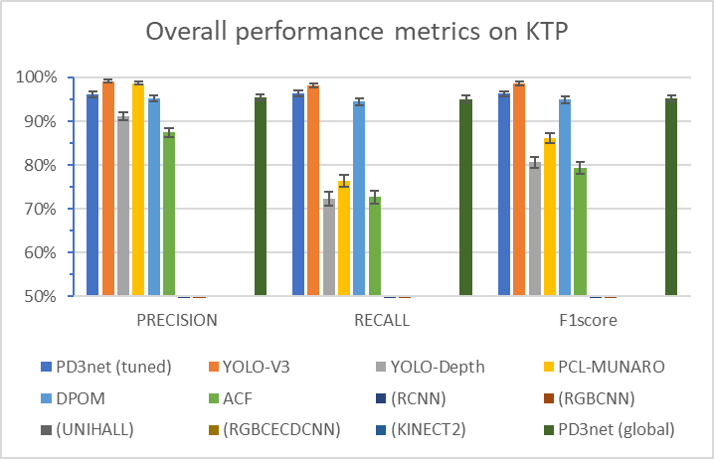
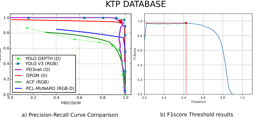
Figure 17 shows the $Precision{}$-$Recall{}$ curve corresponding to the behavior of the five algorithms and the $F_{1score}{}-Threshold$ curve corresponding to the PD3net algorithm. Again, the later curve shows how the working point exhibits a wide flat area, indicating that its sensitivity to the threshold value is small. In addition to this, we can see that YOLO-V3 shows a $Precision{}$-$Recall{}$ curve that is near the perfection in KTP, compared to DPOM or PD3net.

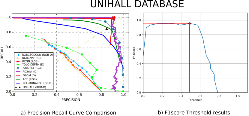
4.4.3 Results for the UNIHALL database

The fourth column of Table 8 and Figure 18 show the results when evaluating on the KTP dataset, using our proposal PD3net, the YOLO-V3 and YOLO-Depth algorithms, and three other proposals from the literature (DPOM, ACF, PCL-MUNARO and KINECT2).

In this case, the PD3net algorithm is the best one in terms of the three evaluated metrics, but its improvement as compared with the second best (DPOM) is not statistically significant.

Figure 18: Results on the UNIHALL dataset.

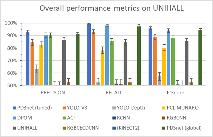
Figure 19 shows the $Precision{}$-$Recall{}$ curve and the $F_{1score}{}$ sweep curve corresponding to PD3net algorithm. With respect to the $F_{1score}{}$ metric, the curve shows a stable working point that falls sharply compared to other databases from a threshold of $0.6$, so we can see that the working point represented by a sharp peak in the $Precision{}$-$Recall{}$ curve is, in fact, a long-range of stable working points. In this case, the $Precision{}$-$Recall{}$ curve clearly shows that the proposed algorithm (PD3net) has the best possible working point, very closely followed as the second-best solution by DPOM and with a large distance in this case to the best third solution represented by YOLO-V3, which is again affected by the presence of strong occlusions in this dataset.

Figure 19: $Precision{}$-$Recall{}$ curve comparison and $F_{1score}{}$-Threshold results for the experiments on the UNIHALL dataset.

4.4.4 Results for the EPFL-LAB database

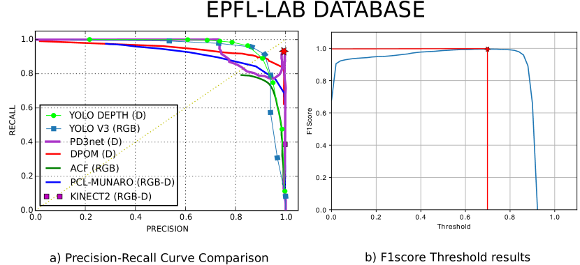
The fifth column of Table 8 and Figure 20 show the results when evaluating on the EPFL-LAB dataset, using our proposal PD3net, the YOLO-V3 and YOLO-Depth algorithms, and seven other proposals from the literature (DPOM, ACF, PCL-MUNARO, RCNN, RGBCNN, RGBCECDCNN, and UNIHALL).

In this case, the PD3net algorithm is the best in terms of the three evaluated metrics, and its improvements as compared with the second best (YOLO-V3) are again, statistically significant.

Figure 20: Results on the EPFL-LAB dataset.

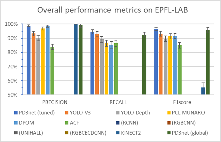
Figure 21 shows the $Precision{}$-$Recall{}$ curve and the $F_{1score}{}$ sweep curve corresponding to PD3net algorithm. Again, the best algorithm in terms of working point in the $Precision{}$-$Recall{}$ curve is PD3net. This curve exhibits a very different behavior from the one seen in previous datasets, forming a very steep slope and peak. To demonstrate that this peak represents a large number of good and stable working points, the $F_{1score}{}$ graph clearly shows how there is a range of threshold values (from $0.6$ to $0.8$ that is practically stable in terms of $F_{1score}{}$.

Figure 21: $Precision{}$-$Recall{}$ curve comparison and $F_{1score}{}$-Threshold results for the experiments on the EPFL-LAB dataset.

4.4.5 Results for the EPFL-CORRIDOR database

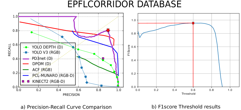
The sixth column of Table 8 and Figure 22 show the results when evaluating on the EPFL-CORRIDOR dataset, using our proposal PD3net, the YOLO-V3 and YOLO-Depth algorithms, and four other proposals from the literature (DPOM, ACF, PCL-MUNARO, and KINECT2 [33]). In this case, the PD3net algorithm is again the best in terms of recall and $F_{1score}{}$ metrics and the third in terms of precision (although the good results in Precision by the DPOM algorithm are related to a poor behaviour in terms of Recall). Its improvements in terms of Recall and $F_{1score}{}$ compared to the second best algorithm (DPOM) are statistically significant.

Figure 22: Results on the EPFL-CORRIDOR dataset.

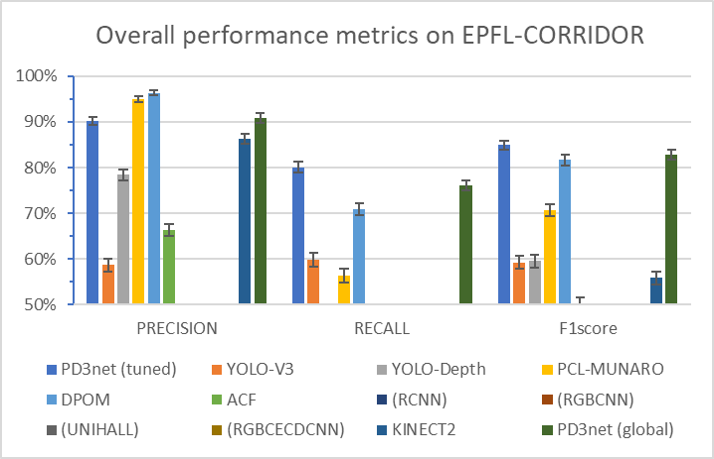
Figure 23 shows the $Precision{}$-$Recall{}$ curve and the $F_{1score}{}$ sweep curve corresponding to PD3net algorithm. EPFL-CORRIDOR is one of the most complex databases, bringing together difficulties such as many occlusions and people very close together, detection in small spaces with a lot of perspectives, great noise in the depth data and many false detections due to people occluded by the image borders. All these issues lead to algorithms like YOLO-V3 to drastically reduce their performance, while PD3net manages to keep a more robust performance, this time with a less stable working point in terms of $F_{1score}{}$, as compared to the results obtained in other databases. The second best system is again DPOM,in this case with significant differences in the results in terms of working point. Finally, in third place we find PCL-MUNARO closely following the DPOM but with remarkable differences in their $Precision{}$-$Recall{}$ curves.

Figure 23: $Precision{}$-$Recall{}$ curve comparison and $F_{1score}{}$-Threshold results for the experiments on the EPFL-CORRIDOR dataset.

4.4.6 Average results for all the available datasets

Table 9 and Figure 24 show the weighted average results when evaluating all the available datasets using all the available algorithms. They have been calculated integrating the results from the above sections, weighting each result according to the number of ground truth elements of each testing subset.

Table 9: Average weighted results using all the available datasets.

	$Precision{}$	$Recall{}$	$F_{1score}{}$
PD3net tuned	$97.51$	222$93.80$	222$95.62\pm 0.24$
PD3net global	222$97.68$	$92.59$	$95.07\pm 0.25$
YOLO-V3	$81.02$	$84.05$	$82.51\pm 0.45$
YOLO-Depth	$80.75$	$57.08$	$66.88\pm 0.55$
PCL-MUNARO	$95.29$	$68.31$	$79.57\pm 0.80$
DPOM	$95.57$	$83.19$	$88.95\pm 0.62$
ACF	$77.67$	$60.35$	$67.92\pm 0.93$
RCNN	$50.10$	$51.40$	$50.74\pm 3.22$
RGBCNN	$49.70$	$51.20$	$50.44\pm 3.22$
UNIHALL	$86.30$	$84.50$	$85.39\pm 2.28$
RGBCECDCNN	$52.30$	$52.30$	$52.30\pm 3.22$
KINECT2	$88.58$	$40.69$	$55.77\pm 1.33$

Figure 24: Average weighted results using all the available datasets.

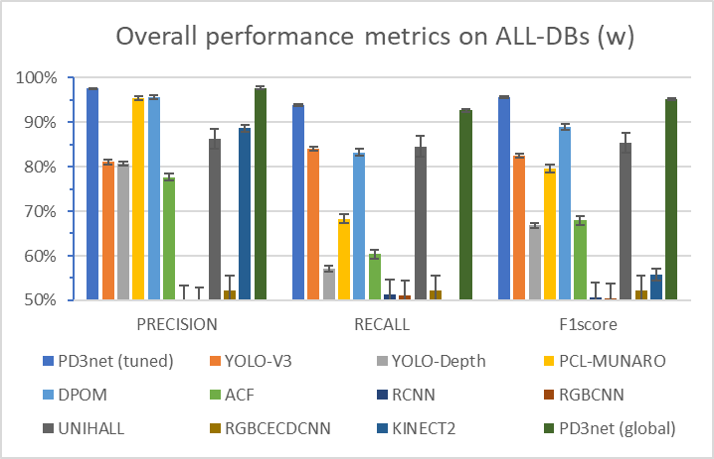
In the average comparison over all the datasets, we can observe that the statistical significance of the results is increased, provided the higher number of considered samples. In terms of $Precision{}$ the best algorithm is PD3net, with DPOM and PCL-MUNARO coming second and third. In terms of $Recall{}$ the differences increase, with a large distance among the first three best proposals. The top system is again PD3net, followed by DPOM and YOLO-V3. Finally, considering the $F_{1score}{}$ that relates the two previous metrics offering a final joint one, PD3net comes first, clearly surpassing DPOM, which is the second-best method with a wide statistical significance.

4.4.7 Discussion on the $Precision{}-Recall{}$ curves for the Global training approach

In this section we provide details on the comparison of our proposal with the other state of the art methods considering the $Precision{}-Recall{}$ and $F_{1score}{}-Threshold$ curves, when the network model and the threshold have been trained using all the available training subsets (referred to as the Global approach in Section 4.2.4.

Figure 25 shows the $Precision$-$Recall$ curves for all the datasets and different algorithms.

Figure 25: $Precision{}$-$Recall{}$ curve comparison using a single global network model and a single global threshold for all datasets.

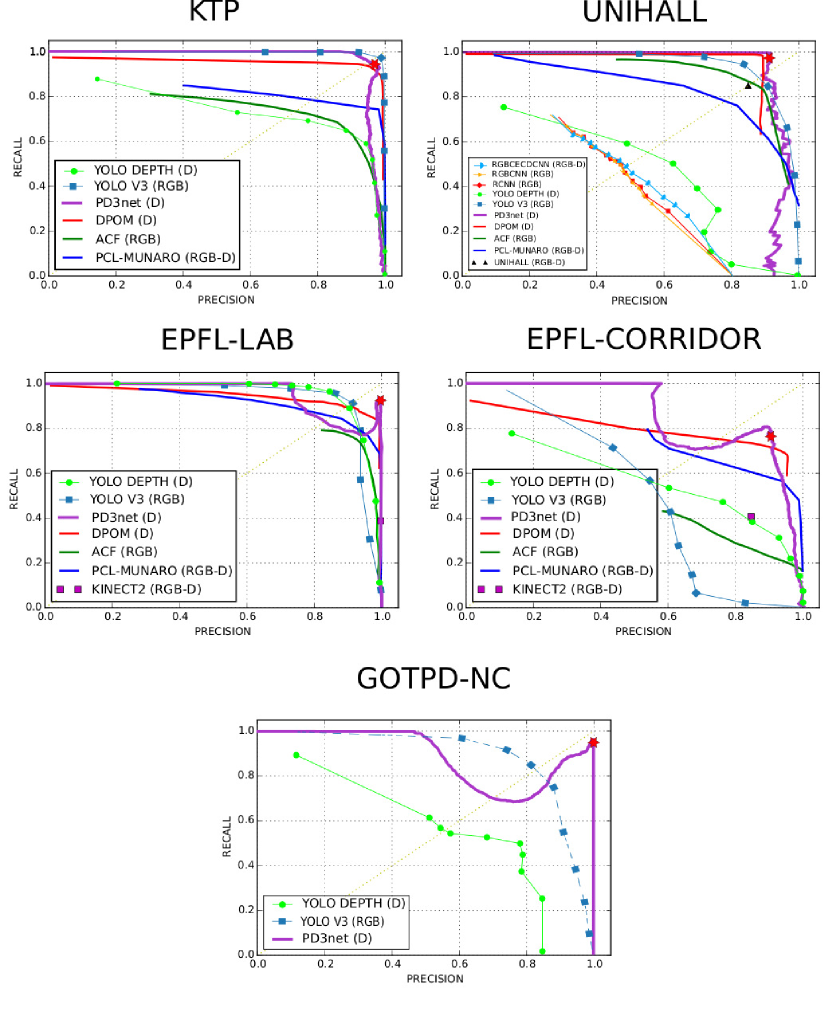
The curves obtained in this case for each dataset are very similar to those found in Figures 15, 17, 19, 21 and 23, which is consistent with the performance metric results in Table 8, which showed non significant differences between the tuned and global approaches.

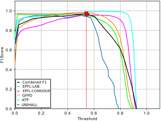
Figure 26 shows the $F_{1score}{}$-Threshold curve for the proposed PD3net algorithm and the different datasets. We also include the average curve (labeled “Combined F1”), from which a single threshold of $0.54$ was selected, as the one with the maximum average $F_{1score}{}$. The fact that this best threshold is located around the middle of the threshold span also supports the robustness of the proposed strategy.

Figure 26: $F_{1score}{}$-Threshold results in the experiments using a single global network model and a single global threshold for all datasets.

4.5 Computational Performance Evaluation

The average frame rate of the system is 42 FPS (frames per second), benchmarked on a conventional Linux desktop PC, with a Processor Intel®Core(TM) i7-6700K CPU @ 4.00 GHz with 64 GB of RAM, and an NVIDIA GTX-1080 TI GPU.

5 Conclusions

This work proposes a new people detection method with depth maps, based in a non-conventional convolutional neural network approximation. This approximation was specifically designed to detect people only using the depth data captured by different types of depth sensor technology(ToF, active stereo, or structured light).

This article includes a very thorough evaluation and comparison with different methods of detection of people from the state of the art, both classical and based on DNN. All this evaluation has been carried out on 5 different RGB-D image databases, each one using a different depth sensor, all this together with a rigorous experimental evaluation process. The scenes used for training and those used for evaluation are as realistic as possible, including a wide variety of users, backgrounds, and elements in them.

The method proposed has been evaluated with a detection threshold for each of the databases and with a common threshold for all of them, making the analysis of the two cases in depth. In addition, an evaluation has been carried out on all the databases and on each one of them specifically highlighting the most important results and details.

In each of the databases used our method obtains if not the best, of the best metrics of all the state of the art systems evaluated, using only depth maps as input. This system beats in many occasions RGB methods that have revolutionized the state of the art like YOLO-V3 or classic methods that use very outstanding depth maps like DPOM. The method used works well even in situations with a large number of users and occlusions.

The proposed method has worked well on three different depth sensor technologies, is quite general in that sense. This method requires training with a synthetically generated database and a small amount of data captured by the camera to allow it to be coupled with reality, but does not require a camera calibration process to know the intrinsic and extrinsic data of the sensor.

6 Acknowledgments

This work has been partially supported by the Spanish Ministry of Economy and Competitiveness under projects HEIMDAL-UAH (TIN2016-75982-C2-1-R) and ARTEMISA (TIN2016-80939-R) and by the University of Alcalá under projects ACERCA (CCG2018/EXP-019) and ACUFANO (CCG19/IA-024).

References

- [1] W. G. Aguilar, M. A. Luna, J. F. Moya, V. Abad, H. Ruiz, H. Parra, and W. Lopez. Cascade classifiers and saliency maps based people detection. In L. T. De Paolis, P. Bourdot, and A. Mongelli, editors, Augmented Reality, Virtual Reality, and Computer Graphics, pages 501–510, Cham, 2017. Springer International Publishing.
- [2] V. Badrinarayanan, A. Kendall, and R. Cipolla. SegNet: A deep convolutional encoder-decoder architecture for image segmentation. CoRR, abs/1511.00561, 2015.
- [3] T. Bagautdinov, F. Fleuret, and P. Fua. Probability occupancy maps for occluded depth images. In 2015 IEEE Conference on Computer Vision and Pattern Recognition (CVPR), pages 2829–2837, June 2015.
- [4] S. Bak, M. San Biagio, R. Kumar, V. Murino, and F. Brémond. Exploiting feature correlations by brownian statistics for people detection and recognition. IEEE Transactions on Systems, Man, and Cybernetics: Systems, 47(9):2538–2549, Sep. 2017.
- [5] Blender Online Community. Blender - a 3D modelling and rendering package, 2018.
- [6] A. Bochkovskiy, C.-Y. Wang, and H.-Y. M. Liao. YOLOv4: Optimal speed and accuracy of object detection, 2020.
- [7] Y. Cao, C. Shen, and H. T. Shen. Exploiting depth from single monocular images for object detection and semantic segmentation. IEEE Transactions on Image Processing, 26(2):836–846, 2017.
- [8] A. Chan, Z.-S. Liang, and N. Vasconcelos. Privacy preserving crowd monitoring: Counting people without people models or tracking. In Computer Vision and Pattern Recognition, 2008. CVPR 2008. IEEE Conference on, pages 1–7, June 2008.
- [9] T.-Y. Chen, C.-H. Chen, D.-J. Wang, and Y.-L. Kuo. A people counting system based on face-detection. In Genetic and Evolutionary Computing (ICGEC), 2010 Fourth International Conference on, pages 699–702, Dec 2010.
- [10] F. Chollet. Xception: Deep learning with depthwise separable convolutions. CoRR, abs/1610.02357, 2016.
- [11] B.-K. Dan, Y.-S. Kim, Suryanto, J.-Y. Jung, and S.-J. Ko. Robust people counting system based on sensor fusion. Consumer Electronics, IEEE Transactions on, 58(3):1013–1021, August 2012.
- [12] L. Del Pizzo, P. Foggia, A. Greco, G. Percannella, and M. Vento. Counting people by RGB or depth overhead cameras. Pattern Recognition Letters, 81(C):41–50, Oct. 2016.
- [13] P. Dollár, R. Appel, and W. Kienzle. Crosstalk cascades for frame-rate pedestrian detection. pages 645–659, 10 2012.
- [14] P. Dollár, Z. Tu, P. Perona, and S. Belongie. Integral channel features. 01 2009.
- [15] X. Du, T.-Y. Lin, P. Jin, G. Ghiasi, M. Tan, Y. Cui, Q. V. Le, and X. Song. SpineNet: Learning scale-permuted backbone for recognition and localization, 2019.
- [16] D. Fuentes-Jiménez, D. Casillas-Pérez, D. Pizarro-Pérez, T. Collins, and A. Bartoli. Deep shape-from-template: Wide-baseline, dense and fast registration and deformable reconstruction from a single image. CoRR, abs/1811.07791, 2018.
- [17] D. Fuentes-Jimenez, C. L. Gutierrez, J. M. Guarasa, C. Luna, and D. Pizarro. Depth person detection database (gfpd-uah).
- [18] D. Fuentes-Jimenez, C. Losada-Gutierrez, and R. Martín-Lopez. GESDPD depth people detection dataset, 2019.
- [19] D. Fuentes-Jimenez, R. Martin-Lopez, C. Losada-Gutierrez, D. Casillas-Perez, J. Macias-Guarasa, C. A. Luna, and D. Pizarro. DPDnet: A robust people detector using deep learning with an overhead depth camera. Expert Systems with Applications, page 113168, 2019.
- [20] F. Galăík and R. Gargalík. Real-time depth map based people counting. In 15th International Conference on Advanced Concepts for Intelligent Vision Systems - Volume 8192, ACIVS 2013, pages 330–341, Berlin, Heidelberg, 2013. Springer-Verlag.
- [21] A. Gavriilidis, J. Velten, S. Tilgner, and A. Kummert. Machine learning for people detection in guidance functionality of enabling health applications by means of cascaded SVM classifiers. Journal of the Franklin Institute, 355(4):2009 – 2021, 2018. Special Issue on Recent advances in machine learning for signal analysis and processing.
- [22] G.Ghiasi, T.Lin, and Q.V.Le. NAS-FPN: Learning scalable feature pyramid architecture for object detection. In 2019 IEEE/CVF Conference on Computer Vision and Pattern Recognition (CVPR), pages 7029–7038, 2019.
- [23] R. B. Girshick, J. Donahue, T. Darrell, and J. Malik. Rich feature hierarchies for accurate object detection and semantic segmentation. CoRR, abs/1311.2524, 2013.
- [24] V. Golyanik, S. Shimada, K. Varanasi, and D. Stricker. HDM-Net: Monocular non-rigid 3D reconstruction with learned deformation model. CoRR, abs/1803.10193, 2018.
- [25] D. Guera and E. J. Delp. Deepfake video detection using recurrent neural networks. 2018 15th IEEE International Conference on Advanced Video and Signal Based Surveillance (AVSS), pages 1–6, 2018.
- [26] T. Hayashi, M. Nishida, N. Kitaoka, and K. Takeda. Daily activity recognition based on dnn using environmental sound and acceleration signals. In 2015 23rd European Signal Processing Conference (EUSIPCO), pages 2306–2310, 2015.
- [27] K. He, X. Zhang, S. Ren, and J. Sun. Deep residual learning for image recognition. In 2016 IEEE Conference on Computer Vision and Pattern Recognition, CVPR 2016, Las Vegas, NV, USA, June 27-30, 2016, pages 770–778, 2016.
- [28] T. Hu, H. Zhang, X. Zhu, J. Clunis, and G. Yang. Depth sensor based human detection for indoor surveillance. Future Generation Computer Systems, 88:540 – 551, 2018.
- [29] Intel. Intel realsense D435 product. https://www.intelrealsense.com/depth-camera-d435/.
- [30] C. Y. Jeong, S. Choi, and S. W. Han. A method for counting moving and stationary people by interest point classification. In Image Processing (ICIP), 2013 20th IEEE International Conference on, pages 4545–4548, Sept 2013.
- [31] N. S. Keskar and R. Socher. Improving generalization performance by switching from adam to SGD. CoRR, abs/1712.07628.
- [32] H. Kim, P. Garrido, A. Tewari, W. Xu, J. Thies, N. Nießner, P. Pérez, C. Richardt, M. Zollhöfer, and C. Theobalt. Deep Video Portraits. ACM Transactions on Graphics 2018 (TOG), 2018.
- [33] Kinect-SDK. Kinect for windows SDK 2.0. http://www.microsoft.com/en-us/kinectforwindows/., 2014.
- [34] D. P. Kingma and J. Ba. Adam: A method for stochastic optimization. CoRR, abs/1412.6980, 2014.
- [35] A. Krizhevsky, I. Sutskever, and G. E. Hinton. ImageNet classification with deep convolutional neural networks. In F. Pereira, C. J. C. Burges, L. Bottou, and K. Q. Weinberger, editors, Advances in Neural Information Processing Systems 25, pages 1097–1105. Curran Associates, Inc., 2012.
- [36] K.-D. Lee, M. Y. Nam, K.-Y. Chung, Y.-H. Lee, and U.-G. Kang. Context and profile based cascade classifier for efficient people detection and safety care system. Multimedia Tools and Applications, 63(1):27–44, 2013.
- [37] T.-Y. Lin, M. Maire, S. Belongie, L. Bourdev, R. Girshick, J. Hays, P. Perona, D. Ramanan, C. L. Zitnick, and P. Dollár. Microsoft COCO: Common objects in context, 2014.
- [38] J. Liu, Y. Liu, G. Zhang, P. Zhu, and Y. Q. Chen. Detecting and tracking people in real time with RGB-D camera. Pattern Recognition Letters, 53:16 – 23, 2015.
- [39] M. Luber, L. Spinello, and K. O. Arras. People tracking in RGB-D data with on-line boosted target models. In 2011 IEEE/RSJ International Conference on Intelligent Robots and Systems, IROS 2011, San Francisco, CA, USA, September 25-30, 2011, pages 3844–3849. IEEE, 2011.
- [40] C. A. Luna, C. Losada-Gutierrez, D. Fuentes-Jimenez, A. Fernandez-Rincon, M. Mazo, and J. Macias-Guarasa. Robust people detection using depth information from an overhead time-of-flight camera. Expert Syst. Appl., 71(C):240–256, Apr. 2017.
- [41] A. Moro, J. Wakabayashi, T. Toda, and K. Umeda. A framework for human recognition and counting in restricted area for video surveillance. In Intelligent Environments (Workshops), pages 139–148, 2018.
- [42] M. Munaro and E. Menegatti. Fast RGB-D people tracking for service robots. Autonomous Robots, 37, 10 2014.
- [43] A. Odena, V. Dumoulin, and C. Olah. Deconvolution and checkerboard artifacts. Distill, 1, 10 2016.
- [44] D. Ramanan, D. A. Forsyth, and A. Zisserman. Tracking People by Learning Their Appearance. Pattern Analysis and Machine Intelligence, IEEE Transactions on, 29(1):65–81, Nov. 2006.
- [45] J. Redmon, S. K. Divvala, R. B. Girshick, and A. Farhadi. You only look once: Unified, real-time object detection. CoRR, abs/1506.02640, 2015.
- [46] J. Redmon and A. Farhadi. YOLOv3: An incremental improvement. CoRR, abs/1804.02767, 2018.
- [47] X. Ren, S. Du, and Y. Zheng. Parallel RCNN: A deep learning method for people detection using rgb-d images. In 2017 10th International Congress on Image and Signal Processing, BioMedical Engineering and Informatics (CISP-BMEI), pages 1–6, Oct 2017.
- [48] E. Romera, J. M. Álvarez, L. M. Bergasa, and R. Arroyo. Efficient convnet for real-time semantic segmentation. In 2017 IEEE Intelligent Vehicles Symposium (IV), pages 1789–1794, June 2017.
- [49] H.-c. Shin, H. Roth, M. Gao, L. Lu, Z. Xu, I. Nogues, J. Yao, D. Mollura, and R. Summers. Deep convolutional neural networks for computer-aided detection: CNN architectures, dataset characteristics and transfer learning. IEEE Transactions on Medical Imaging, 35:1285–1298, 02 2016.
- [50] J. Shotton, A. Fitzgibbon, M. Cook, T. Sharp, M. Finocchio, R. Moore, A. Kipman, and A. Blake. Real-time human pose recognition in parts from single depth images. volume 56, pages 1297–1304, 06 2011.
- [51] L. Spinello and K. O. Arras. People detection in RGB-D data. In 2011 IEEE/RSJ International Conference on Intelligent Robots and Systems, pages 3838–3843, Sep. 2011.
- [52] C. Stahlschmidt, A. Gavriilidis, J. Velten, and A. Kummert. People detection and tracking from a top-view position using a time-of-flight camera. In A. Dziech and A. Czyazwski, editors, Multimedia Communications, Services and Security, volume 368 of Communications in Computer and Information Science, pages 213–223. Springer Berlin Heidelberg, 2013.
- [53] C. Stahlschmidt, A. Gavriilidis, J. Velten, and A. Kummert. Applications for a people detection and tracking algorithm using a time-of-flight camera. Multimedia Tools and Applications, pages 1–18, 2014.
- [54] C. Szegedy, V. Vanhoucke, S. Ioffe, J. Shlens, and Z. Wojna. Rethinking the inception architecture for computer vision. CoRR, abs/1512.00567, 2015.
- [55] Y. Tian, P. Luo, X. Wang, and X. Tang. Pedestrian detection aided by deep learning semantic tasks. In 2015 IEEE Conference on Computer Vision and Pattern Recognition (CVPR), pages 5079–5087, June 2015.
- [56] J. R. R. Uijlings, K. E. A. van de Sande, T. Gevers, and A. W. M. Smeulders. Selective search for object recognition. International Journal of Computer Vision, 104(2):154–171, Sep 2013.
- [57] P. Vera, S. Monjaraz, and J. Salas. Counting pedestrians with a zenithal arrangement of depth cameras. Machine Vision and Applications, 27(2):303–315, Feb 2016.
- [58] N. K. Verma, R. Dev, S. Maurya, N. K. Dhar, and P. Agrawal. People counting with overhead camera using fuzzy-based detector. In N. K. Verma and A. K. Ghosh, editors, Computational Intelligence: Theories, Applications and Future Directions - Volume I, pages 589–601, Singapore, 2019. Springer Singapore.
- [59] M. Villamizar, A. Martínez-González, O. Canévet, and J.-M. Odobez. Watchnet: Efficient and depth-based network for people detection in video surveillance systems. In 2018 15th IEEE International Conference on Advanced Video and Signal Based Surveillance (AVSS), pages 1–6. IEEE, 2018.
- [60] C. Wang and Y. Zhao. Multi-layer proposal network for people counting in crowded scene. In 2017 10th International Conference on Intelligent Computation Technology and Automation (ICICTA), pages 148–151, Oct 2017.
- [61] S. Wang, L. Chen, Z. Zhou, X. Sun, and J. Dong. Human fall detection in surveillance video based on PCANet. Multimedia tools and applications, 75(19):11603–11613, 2016.
- [62] B. Xu, N. Wang, T. Chen, and M. Li. Empirical evaluation of rectified activations in convolutional network. CoRR, abs/1505.00853, 2015.
- [63] L. Zhang, X. Wu, and D. Luo. Human activity recognition with HMM-DNN model. In 2015 IEEE 14th International Conference on Cognitive Informatics & Cognitive Computing (ICCI* CC), pages 192–197. IEEE, 2015.
- [64] S. Zhang, R. Benenson, M. Omran, J. Hosang, and B. Schiele. How far are we from solving pedestrian detection? In Proceedings of the IEEE Conference on Computer Vision and Pattern Recognition, pages 1259–1267, 2016.
- [65] S. Zhang, R. Benenson, M. Omran, J. Hosang, and B. Schiele. Towards reaching human performance in pedestrian detection. IEEE Transactions on Pattern Analysis and Machine Intelligence, 40(4):973–986, April 2018.
- [66] X. Zhang, J. Yan, S. Feng, Z. Lei, D. Yi, and S. Li. Water filling: Unsupervised people counting via vertical Kinect sensor. In Advanced Video and Signal-Based Surveillance (AVSS), 2012 IEEE Ninth International Conference on, pages 215–220, Sept 2012.
- [67] J. Zhao, G. Zhang, L. Tian, and Y. Q. Chen. Real-time human detection with depth camera via a physical radius-depth detector and a CNN descriptor. In 2017 IEEE International Conference on Multimedia and Expo (ICME), pages 1536–1541, July 2017.
- [68] K. Zhou, A. Paiement, and M. Mirmehdi. Detecting humans in RGB-D data with CNNs. In 2017 Fifteenth IAPR International Conference on Machine Vision Applications (MVA), pages 306–309, May 2017.
- [69] K. Zhou, A. Paiement, and M. Mirmehdi. Detecting humans in rgb-d data with cnns. In 2017 Fifteenth IAPR International Conference on Machine Vision Applications (MVA), pages 306–309, May 2017.
- [70] L. Zhu and K.-H. Wong. Human tracking and counting using the kinect range sensor based on adaboost and kalman filter. In International Symposium on Visual Computing, pages 582–591. Springer, 2013.