A Weakly Supervised Region-Based Active Learning Method for COVID-19 Segmentation in CT Images

Abstract

One of the key challenges in the battle against the Coronavirus (COVID-19) pandemic is to detect and quantify the severity of the disease in a timely manner. Computed tomographies (CT) of the lungs are effective for assessing the state of the infection. Unfortunately, labeling CT scans can take a lot of time and effort, with up to 150 minutes per scan. We address this challenge introducing a scalable, fast, and accurate active learning system that accelerates the labeling of CT scan images. Conventionally, active learning methods require the labelers to annotate whole images with full supervision, but that can lead to wasted efforts as many of the annotations could be redundant. Thus, our system presents the annotator with unlabeled regions that promise high information content and low annotation cost. Further, the system allows annotators to label regions using point-level supervision, which is much cheaper to acquire than per-pixel annotations. Our experiments on open-source COVID-19 datasets show that using an entropy-based method to rank unlabeled regions yields to significantly better results than random labeling of these regions. Also, we show that labeling small regions of images is more efficient than labeling whole images. Finally, we show that with only 7% of the labeling effort required to label the whole training set gives us around 90% of the performance obtained by training the model on the fully annotated training set. Code is available at: https://github.com/IssamLaradji/covid19_active_learning.

1 Introduction

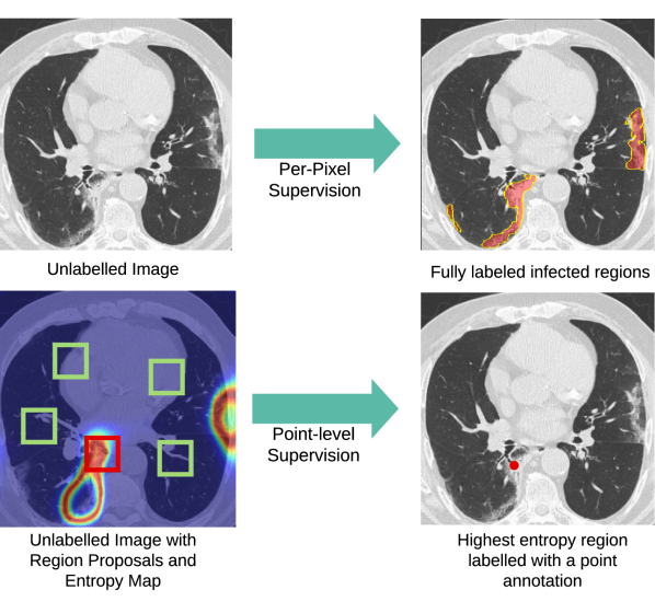
Figure 1: Labeling Schemes. (Top) Conventional per-pixel labeling of the whole image. (Bottom) Our proposed region-based labeling scheme with point-level supervision. The region with the highest entropy (shown within the red rectangle) is labeled by clicking on a single pixel that is on top of an infected region.

The Severe Acute Respiratory Syndrome Coronavirus 2 (SARS-CoV-2) has rapidly spread into a pandemic and overwhelmed healthcare centers around the world. While the disease (COVID-19) presents with a variety of symptoms, the build up of fluid in a patient’s lungs has been most commonly associated with morbidity and mortality. These affected regions, which are known as pulmonary opacification [23], present as various patterns of attenuation on CT imaging and have been correlated with the severity of the COVID-19 infection [32, 55]. In severe cases, treatment of the disease requires intervention with essential equipment, which has lead to shortages around the world. Accurate and accessible diagnostic methods are necessary to slow the spread of the virus, and efficient methods for prognosis and treatment are needed to ease the burden on healthcare centres in heavily affected regions.

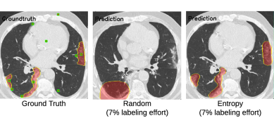
Figure 2: Prediction comparison between fully supervised and region-based active learning system. With only 7% of the labeling effort (columns 2 and 3), segmented regions are close to the ground truth labels baseline (column 1). The points in column 1 represents example point-level annotations on infected regions and background.

RT-PCR (Reverse Transcription-Polymerase Chain Reaction) has emerged as the standard screening protocol for COVID-19, however it is time consuming and has a high false-negative rate [63]. Recent work has shown that the analysis patterns of pulmonary opacification on chest CT scans provides a complementary screening protocol that achieves sensitive diagnosis [1]. Additionally, recent work has shown that quantification of pulmonary opacification allows for the prognostication of patients, as the percentage of well-aerated-lung has been shown to be a predictive measure of intensive care unit (ICU) admission and death [10] . In areas with concentrated COVID-19 infections, radiologists are burdened with the time consuming task of analyzing CT scans. To this end, we investigate AI-based models for the segmentation of pulmonary opacification, thus significantly reducing the burden on healthcare centers and providing important information for the diagnosis and prognosis of COVID-19 patients.

Thus, we consider deep learning methods, which is a class of AI that has been successful in the medical imaging field for diagnosis, monitoring, and treatment of a variety of infections. Deep learning has already been applied to the medical image segmentation the brain [12, 9] lung [24], and pancreas [42]. The goal is to assign a class label to each pixel in the images, which involves detecting unhealthy tissues or the areas of interest. The classical U-Net [41] is one of the main deep learning segmentation methods that was shown to achieve promising performance in medical segmentation. Extensions to U-Net emerged to tackle medical segmentation using methods that are based on attention and multi-tasking [5]. Overall, deep learning-based methods consistently outperform traditional methods in the medical image segmentation task.

Recently, deep learning methods were used to help in the diagnosis of COVID-19 infections [31, 6, 57, 53]. These methods range from standard architectures to anomaly detection models designed to help radiologists analyze chest X-ray images. For CT images, segmenting COVID-19 infections was performed using location-attention oriented, 3D CT volume-based [60], and edge detection based models [17]. However, these methods do not consider model’s feedback when labeling the training set, leading to possibly inefficient efforts as some training images might have redundant information.

According to Ma et al. [36], it takes around 400 minutes to delineate one CT scan with 250 slices. It is important that only the scans that maximize the model’s performance are labeled for cost efficiency. We address this challenge by introducing an active learning system combined with weak supervision. Active learning (AL) is a popular procedure to select the most informative images to label. The goal is to maximize the validation score with as few images labeled as possible. The information of an unlabeled image is often measured using entropy, which estimates the uncertainty of a model’s output on that image. This approach has been beneficial for semantic segmentation [37]. Similar to Mackowiak et al. [37], Casanova et al. [7], our active learning system only presents parts of the unlabeled image to the annotator for labeling (Figure 1). It was shown that it is easier for the annotator to label regions and allows the annotators to further focus their efforts on labeling the most informative image patches.

These methods, however, require the annotator to label each region with per-pixel labels. This labeling scheme leads to two main challenges. First, per-pixel labels require a lot of effort. Second, under the active learning setup, it is difficult to calculate how much effort each region requires. Background regions require less effort to label than having to draw boundaries around infected regions. In Mackowiak et al. [37], Casanova et al. [7], effort was measured based on the percentage of pixels labeled, which is not accurate.

For our active learning system, the annotator is allowed to label uninfected regions with the background tag and regions with infections by placing a single click randomly on an infection. This scheme is also much faster to acquire than per-pixel labels, and we can accurately assume similar efforts between regions.

We evaluated our active learning framework on the publicly available CT Scan datasets. Our work follows the common AL setup where training is made of cycles, and in each cycle a set of images is selected for labeling [45]. In each cycle the trained model computes an uncertainty map on the unlabeled regions first. Then, a set of unlabeled regions are sampled based on their uncertainty scores so that the more uncertain ones are labeled first. This procedure completes one cycle, and it is repeated until the annotation budget is reached. The intuition behind this method is that it allows the model to learn from low-effort highly informative regions to learn to perform good segmentation.

We summarize our contributions and results on the COVID-19 benchmarks as follows:

1. We propose the first framework that combines region-based active learning with point-level supervision.

2. For the COVID-19 datasets, we show that using an entropy-based method to rank unlabeled regions yields to significantly better results than random labeling of these regions when fixing the annotation budget.

3. For the same datasets, we show that region-based active learning leads to better results compared to whole image labeling.

4. We show the point-level supervision yields better performance with respect to budget compared to per-pixel annotation.

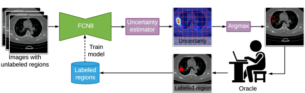
Figure 3: Active Learning Setup. 1. We train the model on the labeled dataset. 2. The trained model is used to estimate the uncertainty on all unlabeled images. 3. The K most uncertain regions are selected and labeled with point-level supervision. 4. The newly labeled examples are added to the dataset for the next training cycle.

2 Related Work

This work falls under the intersection between active learning, weakly supervised and semantic segmentation. We review the relevant work for each of these topics below.

Active learning

aims to maximize the performance on the test set with respect to the number of labeled examples. Different methods exist for selecting which data to be labeled from the unlabeled pool. These methods can be categorized into two categories. First, classical methods include query-by-committee [11, 18], and ensemble disagreement [3]. Secondly, Bayesian methods propose to sample from the posterior distribution before applying an heuristic on the set of predictions. Examples of the latter include Maddox et al. [38], Gal and Ghahramani [19]. Moreover, different heuristics have been proposed to decide which samples to be labeled. These heuristics decide based on different strategies such as entropy [48], maximizing the error reduction [43], or information theory [20, 25]. The heuristics are often used to compute an uncertainty value for the whole image, whereas in this work we compute the entropy for different regions in the image to identify which object instances require per-pixel labels.

Active learning for semantic segmentation

is relatively less explored compared to classification, perhaps because of its challenging large-scale nature. Methods that work on this setup [15] combine metrics that encourage the diversity and representativeness of labeled samples. Some rely on unsupervised superpixel-based over-segmentation [51, 28]. Others focus on foreground-background segmentation of biomedical images [22, 58]. Settles et al. [46], Vijayanarasimhan and Grauman [52], and  [37] focus on cost-effective approaches, proposing manually-designed acquisition functions based on the cost of labeling images or regions of images.

Recent work on active learning with semantic segmentation relies on dividing the images into fixed-sized regions [37, 7] and labeling the highest scoring ones with per-pixel labels. Unfortunately, these methods have two drawbacks. First, the size of the regions need to be predefined and the size can affect the performance widely. In many cases, it is more cost-effective to simply label a single object than a square region. Further, computing the labeling effort for a region is complicated. In Mackowiak et al. [37], Casanova et al. [7], the labeling effort of these regions is assumed to be the same, which is not always the case. Regions that have a single object class are much easier to label than regions with more than one object class. Second, per-pixel labels can be less cost-effective than weaker labels.

Active learning for medical segmentation

has received a lot of attention lately due to its potential in reducing the amount of human effort required to obtain a good training set. Acquiring medical datasets is difficult because it requires expert labelers (doctors) and long annotation time. As a result, there is a limited amount of labeled medical datasets compared to datasets from other domains. Gorriz et al. [21] proposes to use the well-known CEAL method [54] where uncertain examples are labeled by a human and confident examples are labeled by the model. They use U-Net [41] with MC-Dropout [19] and estimate the uncertainty using the predictive variance. Yang et al. [58] train an ensemble network and compute the similarity between features to estimate uncertainty. If the feature vectors are similar, the sample is easy and should not be annotated.

Weak supervision for semantic segmentation

can vastly reduce the required annotation cost for collecting a training set [61, 26, 62, 29, 30]. Collecting image-level and point-level labels for the PASCAL VOC dataset [16] takes only $20.0$ and $22.1$ seconds per image, respectively Bearman et al. [2]. In comparison, acquiring full segmentation labels can take $239.0$ seconds per image on average. Other forms of weaker labels were explored as well, including bounding boxes [26] and image-level annotation [61]. In this work, the labels are given as point-level annotations instead of the conventional per-pixel level labels.

Active learning with weak supervision

is a relatively new research area. To the best of our knowledge, it has only been investigated for the task of object detection [8, 14, 4]. Chandra et al. [8] and Desai et al. [14] have proposed frameworks to use a combination of strong supervision and weak labels in the training process. Leveraging weak labels was shown to reduce the required annotation budget to attain good performance in the active learning setup for object detection. However, strong supervision was still required at the later stages of the training in order to achieve the optimal performance.

Chandra et al. [8] have proposed a two-stage sampling method that is performed in every active learning cycle. In the first stage, images are sampled from the unlabeled data for which the oracle provides weak labels. In the second stage, images are sampled from the weakly labeled data for which the oracle provides strong labels. Desai et al. [14] have proposed an adaptive supervision method. By default the query is sampled from the unlabeled data and the oracle provides the weak labels. There are two conditions that define which level of supervision to use. For the first condition, if the prediction confidence is lower than a certain threshold, the images acquired in the current cycle are labeled with full supervision. The level of supervision for the second condition is based on the value of the loss. In our work, we are the first to combine region-based active learning with point-level supervision and apply it on the task of medical segmentation.

3 Methodology

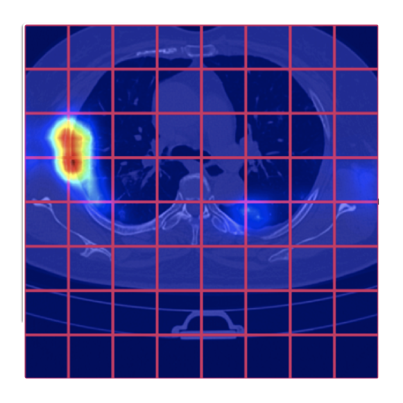
Figure 4: Region-based Labeling. This image is divided into 64 equally-sized non-overlapping rectangles, where each rectangle represents an unlabeled region. The region that has the highest per-pixel entropy mean (shown as heatmap) is selected for labeling.

Setup.

As shown in Figure 3, we follow the common active learning setup where images are divided into labeled $\mathcal{X}_{l}$ and unlabeled $\mathcal{X}_{u}$ images. The process is divided into cycles. In each cycle the model is trained on $\mathcal{X}_{l}$ until convergence before the next batch of unlabeled examples are sampled from $\mathcal{X}_{u}$ for labeling. In the conventional active learning setup, the annotator is required to annotate every pixel in each sampled unlabeled image. This process might not be cost efficient as some regions could be very costly to label while having only little positive impact on the model’s performance. Thus, we instead reformulate the problem by dividing each image into a grid of $K$ equal-sized rectangles as possible regions for labeling (see Figure 4). In this case, the dataset is divided into $\mathcal{X}_{l}$, $\mathcal{X}_{p}$, and $\mathcal{X}_{u}$ where $\mathcal{X}_{p}$ is a set of partially labeled images. In each cycle, regions are sampled from the images $\mathcal{X}_{p}$, and $\mathcal{X}_{u}$ and are then passed to a human oracle for labeling. These regions are selected based on either random or entropy-based heuristics. The latter heuristic allows the model to determine which regions it is mostly uncertain about, which can help improve its generalization performance when labeled.

Labeling Scheme.

We consider two labeling methods: per-pixel and point-level. For per-pixel labels, the annotator is asked to label an object so that each of its pixels are annotated. Given $X$ as a set of $N$ training images with corresponding ground truth labels $Y$. $Y_{i}$ is a $W\times H$ matrix with the value of each entry corresponding to the class label.

When labelers are presented with an unlabeled region, they are only required to annotate that region with per-pixel labels (Figure 1). However, this type of annotation is costly because it requires the labeler to carefully draw a boundary around the object while dealing with occlusions and potential overlapping objects. According to the authors of the COCO dataset [33], it took around 22 worker hours for 1,000 segmentations. This annotation time implies a mean labeling effort of 79 seconds per object segmentation. Also, according to Ma et al. [36], it takes around 400 minutes to delineate one CT scan with 250 slices. That is an average of 1.6 minutes per slice. While this labeling scheme is highly expressive, the information content it provides to the model might not be worth the labeling cost.

Thus, we also consider point-level labels. This labeling scheme allows the annotator to label a single point for each infected region. If the region has no infection, then the annotator is required to classify it as background. The ground truth mask $Y_{i}$ is a $W\times H$ matrix with entries 1 that indicate the locations of the infected regions, entries 0 that indicate background regions, and -1 that indicated unlabeled regions. The annotation cost for each region is similar.

Model Architecture.

We use a segmentation network based on FCN8 [34] with an ImageNet [13] pretrained backbone. The network takes as input an image of size $W\times H$ and applies the forward function $f_{\theta}$, producing a $W\times H\times C$ per-pixel map where $C$ is the set of object classes of interest and $\theta$ are the network parameters. The output map is converted to a per-pixel probability matrix $S_{i}$ by applying the softmax function across these classes. These probabilities indicate the likelihood for each pixel of belonging to the infected region of a class $c\in C$. At test time, for each pixel, the class with the highest probability is selected.

Loss Function for Point-level Supervision.

We apply the standard cross-entropy function against the provided set of point-level annotations which represent the locations of the infected regions and the background pixels. The loss function is defined as follows,

$$\mathcal{L}_{P}(f_{\theta},X_{i},Y_{i})=-\sum_{j\in\mathcal{I}_{i}}\log(f_{\theta}(X_{i})_{jY_{j}})\;,$$ (1)

where $f_{\theta}(X_{i})_{jY_{j}}$ is the output corresponding to class $Y_{j}$ for pixel $j$, and $\mathcal{I}_{i}$ is the set of labeled pixels for image $X_{i}$.

Region-Selection methods.

In each cycle we select regions based on random, or entropy [19] heuristics. With the random heuristic, regions are sampled randomly from $X_{p}$ and $X_{u}$. With the entropy heuristic, the regions with the highest mean per-pixel entropy are selected.

In order to obtain uncertainty measures based on the entropy of the semantic segmentation predictions, we add a dropout layer after fc6 and fc7 in the VGG16 [50] architecture. Using MC-Dropout [19], we acquire $I$ predictions drawn from the posterior distribution,

$$S_{ij}=f(x_{i},\theta_{j})\mid\theta_{j}\sim p(\theta\mid\mathcal{L}),$$ (2)

where $S_{i}j$ is the predicted distribution per pixel for a model $f$ and an input $x_{i}$. This function allows us to select informative images for labeling. The intuition behind MC-Dropout is that if the knowledge of the network about a visual pattern is precise, the predictions should not diverge if the image is evaluated several times by dropping weights randomly at each time.

We estimate the per pixel uncertainty by computing the entropy of the mean estimator. Let $\hat{S_{i}}$ be the mean estimation over $I$ draws. We compute the uncertainty with: $U_{i}=\sum_{c}^{C}S_{ic}\log(S_{ic})$.

Model Training.

We start with an empty set of labeled images $X_{l}=\phi$. Then, we randomly sample an initial set of images and label them with per-pixel labels. Whenever we acquire a new labeled batch we train the model until convergence. In each cycle we compute the per-pixel entropy for for all unlabeled and partially labeled images. The score of each unlabeled region is the maximum pixel entropy within that region. The score of an image is the score of the region with maximum score. Images with unlabeled regions are then ranked based on their score. We then pick the K highest ranked images and select the highest scoring region from each image to labeled with point-level supervision. We terminate the training procedure after $T$ cycles.

Implementation Details

Our methods use an Imagenet-pretrained VGG16 [49] FCN8 network [34]. Other Imagenet-pretrained architectures can be used as well, but we did not observe a difference in the results compared to other architectures such as UNet [41] and PSPNet [59]. We ran the active learning procedure for 100 cycles. In the first cycle, 5 CT images were randomly sampled from the unlabeled pool and all their regions were labeled based on the required supervision level. Each image is divided into 64 equally-sized non-overlapping regions. In each cycle, 5 images are sampled from the unlabeled pool and for each of these images, a single region gets selected for labeling. The maximum number of training epochs in a cycle is 40. The score is reported on the test set and it corresponds to the model that achieved the best score on the validation set. The models are trained with a batch size of 1 using the ADAM [27] optimizer with a learning rate of $10^{-4}$. To compute the uncertainty scores of an image, we perform Monte-Carlo with samples following the procedure in Gal and Ghahramani [19]. The dropout rate was set to 0.5.

Table 1: Statistics of COVID-19 datasets.

Name	# Cases	# Slices	# Slices with	# Infected
			Infections (%)	Regions
COVID-19-A	9	829	372 (44.9%)	1488
COVID-19-B	20	3520	1841 (52.3%)	5608

4 Experimental Setup

4.1 Datasets

We evaluate our system on two open source datasets (COVID-19-A/B) whose statistics are shown in Table 1.

COVID-19-A [39]

consists of 9 volumetric COVID-19 chest CTs in DICOM format containing a total of 829 axial slices. Images were first converted from Houndsfield units to unsigned 8-bit integers, then resized to $352\times 352$ pixels and normalized using ImageNet dataset statistics [44]. Each axial CT slice was labeled for ground-glass, consolidation, and pleural effusion by a radiologist. We use two splits of the dataset: separate and mixed. In the separate split (COVID-19-A-Sep), the slices in the training, validation, and test set come from different scans. The goal is to evaluate how the model generalizes to new patients. In this setup, the first 5 scans are defined as training set, the 6th as validation, and the remaining as test. For the mixed split (COVID-19-A-Mixed), the slices in the training, validation, and test set come from the same scans. The idea is to evaluate if given few labelled slices from a scan the model can infer the masks for the remaining slices. For each scan, the first 45% slices are defined as the training set, the next 5% as the validation, and the remaining as test.

COVID-19-B [35]

consists of 20 COVID-19 CT volumes. Lungs and areas of infection were labeled by two radiologists and verified by an experienced radiologist. Each three-dimensional CT volume was converted from Houndsfield units to unsigned 8-bit integers and normalized using ImageNet data statistics [44]. We also split the dataset into separate and mixed versions. For the separate split (COVID-19-B-Sep), we assign 15 scans to the training set, 1 to the validation set, and 4 to the test set. For the mixed split (COVID-19-B-Mixed), we separate the slices from each scan in the same manner as for COVID-19-A.

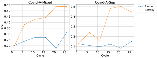
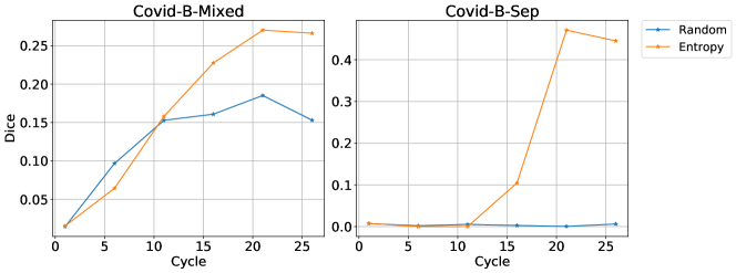
Figure 5: Comparison between random and entropy heuristics. In each cycle, 5 regions were selected for labeling with point-level annotations. Each image is divided into 64 regions. Entropy significantly outperforms random as random tends to select background regions as there is a large imbalance between background and regions with infections.

4.2 Evaluation Metrics

As common practice [47], we evaluate our models using the dice coefficient metric (also known as the F1 Score) for semantic segmentation. Dice is similar to Intersection over Union (IoU) [16] but gives more weight to the intersection between the prediction and the ground truth mask, which is computed as $\text{DICE}=\frac{2*TP}{2*TP+FP+FN}$, where TP, FP, and FN is the number of true positive, false positive and false negative pixels across all images in the test set. We also report results with respect to specificity (true negative rate), $Specificity=\frac{TN}{FP+TN}$, which measures the fraction of real negative samples that were predicted correctly.

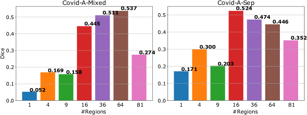
Figure 6: Comparison between different region sizes. For each bar in the plot, the number of regions defines the number of equally-sized non-overlapping rectangles that divide the training images (see rectangle grid in Figure 3). So higher number of regions means that the regions are of smaller size.

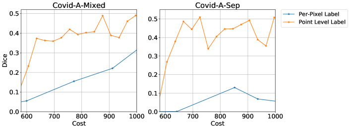
Figure 7: Comparison between point-level and per-pixel level supervision based on 64 regions per image. The cost for a single point annotation is approximated to be 3 seconds [40]. The cost for labeling an infected region is the number of points required to form an approximated polygon around that infection (although in reality it could take more time than that).

5 Experimental Results

5.1 Comparing Entropy against Random Heuristic

For this experiment, a sampled region is labeled in one of two ways depending on whether it contains an infected region. If it has no infected region, then it is labeled with the tag background; otherwise the label is a random point annotation on top of an infected region.

The effort required to label a region in either of these two cases is similar. Thus we plot the obtained results regarding the number of labeled regions against the achieved dice score with the trained FCN. We observe in Figure 5 that entropy significantly outperforms the random heuristic for COVID-19-A and COVID-19-B. The reason is that there are many background regions in these two datasets and thus random is more likely to select only background regions, leading to a poor performance. On the other hand, random sampling obtains a good specificity curve ranging between 0.85 and 0.99 as it maintains a high true negative rate. However, false negatives can cost people’s lives. Thus it is important to have high recall as well, as achieved with entropy sampling. In other words, as shown in the qualitative results, entropy tends to pick infected regions, as it is where the model is mostly uncertain about.

For the separate splits of COVID-19-A and COVID-19-B, there is a bigger margin between random and entropy and that is because the distribution between the training and testing set is more different than in the mixed splits where slices come from the same scans instead. This result suggests a good promise with using region-based active learning with entropy and point-level supervision.

5.2 Effect of Region Size on Performance

In this section, we study the impact of the region size on the Dice score performance. The images are divided into $K$ equally-sized non-overlapping regions, so higher number of regions means the regions are of smaller size. In the first cycle, we chose a budget of 192 seconds to label the initial set of images. For images with 64 regions that corresponds to 3 images ($64\cdot 3$). Thus, more images are fully labeled for those with smaller number of regions.

Figure 6 shows that the region size can have a strong impact on the dice performance. Thus, it is important to carefully choose the right region size when using the presented active learning system. For instance, bigger region sizes led to significantly worse performance. The reason is that the annotations might not be placed in the location that could provide the most informative content for the model. Smaller regions focus on where the model is specifically confused at. Further, if the model is confused about the background, selected smaller regions are more likely to contain only background, which provides a strong signal for background.

5.3 Comparing point-level against per-pixel level supervision

Here we compare the two labeling schemes: (1) per-pixel label scheme, that is full supervision, and (2) the point-level label scheme. We compute the estimated labeling cost as follows. For the point-level labeler it takes around 3 seconds to make a single point annotation [40]. For the per-pixel labeler we approximate the polygon around the infected mask and use its vertices as the number of points required to annotate that mask. The total effort of labeling the mask is 3 seconds (the cost of a single point label) multiplied by the number of vertices. This cost estimation allows us to compare between the two labeling schemes with respect to the obtained performance.

For the per-pixel level loss function, we combine the weighted cross-entropy and IoU loss as defined in Eq. (3) and (5) from Wei et al. [56], respectively. It is an efficient method for ground truth segmentation masks that are imbalanced. Since this loss function requires full supervision, it serves as an upper bound performance in our results.

Figure 7 shows that Point-level labeling achieves superior performance compared to per-pixel labels with lower cost. Each region annotated with per-pixel labels leads to a large increase in labeling cost. Thus, with a fixed annotation budget only few regions can be labeled per-pixel compared with point-level. This result suggests that having more labeled regions with weaker supervision leads to higher overall information content.

Comparison against the upper bound.

We trained the model on the full training set with full supervision on COVID-19-A-Mixed and obtained 84% Dice score. The total labeling cost is 35328 seconds as the training set consists of 368 slices and it takes around 96 seconds to label a slice accurately [36]. With our weakly-supervised active learning system and using entropy as our region-selection heuristic, we achieved 76% dice score (which is around 90% of the upper bound result) with an effort of 2460 seconds (which is 7% of the original effort). Figure 2 shows qualitative results that illustrate that entropy significantly outperforms random with that amount of labeling. For this active learning setup, 5 images were labeled with point-level supervision in the initial cycle. Each image in the training set is divided into 64 regions, leading to an initial effort of $5\cdot 3\cdot 64$ seconds. In each cycle, for 100 cycles, we labeled 5 regions with point-level annotations, leading to a total cost of $5\cdot 3\cdot 64+100\cdot 5\cdot 3=2460$. This result suggests that we can achieve a strong performance with very low human effort.

6 Conclusion

We have proposed a weakly supervised region-based active learning setup for cost-efficient labeling of COVID19 infections in CT scans. This framework combines two ideas for reducing labeling effort. The first idea is to use a region-based active learning approach which, different from conventional active learning, presents the annotator with regions of the image for instead of the whole image. Using entropy-based MCMC, this scheme encourages labeling highly informative regions that maximize the model’s validation accuracy. The second idea is to use point-level supervision which is much cheaper to acquire than per-pixel labels. Since this labeling scheme requires the annotator to label each infected region with a single click, it only requires 3 seconds per infected region. Our results show that entropy-based heuristics outperform random selection of regions with respect to the dice score and labeling effort. Moreover, we show that region-based annotation outperforms whole image labeling in terms of cost efficiency. As a result, our system reaches around 90% of the dice score of the same model trained on the whole training set with only 7% of the effort. For future work, it would be interesting to investigate other forms of weak supervision and other forms of regions that are not rectangles. Such regions could include super pixels or selective search proposals.

References

- Ai et al. [2020] T. Ai, Z. Yang, H. Hou, C. Zhan, C. Chen, W. Lv, Q. Tao, Z. Sun, and L. Xia. Correlation of chest ct and rt-pcr testing in coronavirus disease 2019 (covid-19) in china: a report of 1014 cases. Radiology, page 200642, 2020.
- Bearman et al. [2016] A. Bearman, O. Russakovsky, V. Ferrari, and L. Fei-Fei. What’s the point: Semantic segmentation with point supervision. ECCV, 2016.
- Beluch et al. [2018] W. H. Beluch, T. Genewein, A. Nürnberger, and J. M. Köhler. The power of ensembles for active learning in image classification. In Proceedings of the IEEE Conference on Computer Vision and Pattern Recognition, pages 9368–9377, 2018.
- Brust et al. [2020] C.-A. Brust, C. Käding, and J. Denzler. Active and incremental learning with weak supervision. KI - Künstliche Intelligenz, Jan 2020. ISSN 1610-1987. doi: 10.1007/s13218-020-00631-4. URL http://dx.doi.org/10.1007/s13218-020-00631-4.
- Bui et al. [2019] T. D. Bui, L. Wang, J. Chen, W. Lin, G. Li, and D. Shen. Multi-task learning for neonatal brain segmentation using 3d dense-unet with dense attention guided by geodesic distance. In Domain Adaptation and Representation Transfer and Medical Image Learning with Less Labels and Imperfect Data, pages 243–251. Springer, 2019.
- Butt et al. [2020] C. Butt, J. Gill, D. Chun, and B. A. Babu. Deep learning system to screen coronavirus disease 2019 pneumonia. Applied Intelligence, page 1, 2020.
- Casanova et al. [2020] A. Casanova, P. H. O. Pinheiro, N. Rostamzadeh, and C. J. Pal. Reinforced active learning for image segmentation. In ICLR, 2020.
- Chandra et al. [2020] A. L. Chandra, S. V. Desai, V. N. Balasubramanian, S. Ninomiya, and W. Guo. Active learning with point supervision for cost-effective panicle detection in cereal crops. Plant Methods, 16(1), Mar 2020. ISSN 1746-4811. doi: 10.1186/s13007-020-00575-8. URL http://dx.doi.org/10.1186/s13007-020-00575-8.
- Chen et al. [2018] H. Chen, Q. Dou, L. Yu, J. Qin, and P.-A. Heng. Voxresnet: Deep voxelwise residual networks for brain segmentation from 3d mr images. NeuroImage, 170:446–455, 2018.
- Colombi et al. [2020] D. Colombi, F. C. Bodini, M. Petrini, G. Maffi, N. Morelli, G. Milanese, M. J. Silva, N. Sverzellati, and E. Michieletti. Well-aerated lung on admitting chest ct to predict adverse outcome in covid-19 pneumonia. Radiology, 2020.
- Dagan and Engelson [1995] I. Dagan and S. P. Engelson. Committee-based sampling for training probabilistic classifiers. In ICML, 1995.
- de Brebisson and Montana [2015] A. de Brebisson and G. Montana. Deep neural networks for anatomical brain segmentation. In Proceedings of the IEEE conference on computer vision and pattern recognition workshops, pages 20–28, 2015.
- Deng et al. [2009] J. Deng, W. Dong, R. Socher, L.-J. Li, K. Li, and L. Fei-Fei. ImageNet: A Large-Scale Hierarchical Image Database. In CVPR, 2009.
- Desai et al. [2019] S. V. Desai, A. C. Lagandula, W. Guo, S. Ninomiya, and V. N. Balasubramanian. An adaptive supervision framework for active learning in object detection. arXiv preprint arXiv:1908.02454, 2019.
- Dutt Jain and Grauman [2016] S. Dutt Jain and K. Grauman. Active image segmentation propagation. In CVPR, 2016.
- Everingham et al. [2010] M. Everingham, L. Van Gool, C. K. Williams, J. Winn, and A. Zisserman. The pascal visual object classes (voc) challenge. IJCV, 2010.
- Fan et al. [2020] D.-P. Fan, T. Zhou, G.-P. Ji, Y. Zhou, G. Chen, H. Fu, J. Shen, and L. Shao. Inf-net: Automatic covid-19 lung infection segmentation from ct scans. arXiv preprint arXiv:2004.14133, 2020.
- Freund et al. [1993] Y. Freund, H. S. Seung, E. Shamir, and N. Tishby. Information, Prediction, and Query by Committee. In NIPS, 1993.
- Gal and Ghahramani [2016] Y. Gal and Z. Ghahramani. Dropout as a bayesian approximation: Representing model uncertainty in deep learning. In international conference on machine learning, pages 1050–1059, 2016.
- Gal et al. [2017] Y. Gal, R. Islam, and Z. Ghahramani. Deep bayesian active learning with image data. ICML, 2017.
- Gorriz et al. [2017a] M. Gorriz, A. Carlier, E. Faure, and X. Giró i Nieto. Cost-effective active learning for melanoma segmentation. ML4H: Machine Learning for Health Workshop at NIPS, 2017a.
- Gorriz et al. [2017b] M. Gorriz, A. Carlier, E. Faure, and X. Giró i Nieto. Cost-effective active learning for melanoma segmentation. ML4H: Machine Learning for Health Workshop, NIPS, 2017b.
- Hansell et al. [2008] D. M. Hansell, A. A. Bankier, H. MacMahon, T. C. McLoud, N. L. Müller, and J. Remy. Fleischner society: Glossary of terms for thoracic imaging. Radiology, 246(3):697–722, Mar. 2008. doi: 10.1148/radiol.2462070712. URL https://doi.org/10.1148/radiol.2462070712.
- Harrison et al. [2017] A. P. Harrison, Z. Xu, K. George, L. Lu, R. M. Summers, and D. J. Mollura. Progressive and multi-path holistically nested neural networks for pathological lung segmentation from ct images. In International conference on medical image computing and computer-assisted intervention, pages 621–629. Springer, 2017.
- Houlsby et al. [2011] N. Houlsby, F. Huszár, Z. Ghahramani, and M. Lengyel. Bayesian active learning for classification and preference learning. arXiv preprint arXiv:1112.5745, 2011.
- Khoreva et al. [2017] A. Khoreva, R. Benenson, J. H. Hosang, M. Hein, and B. Schiele. Simple does it: Weakly supervised instance and semantic segmentation. CVPR, 2017.
- Kingma and Ba [2015] D. P. Kingma and J. Ba. Adam: A method for stochastic optimization. ICLR, 2015.
- Konyushkova et al. [2015] K. Konyushkova, R. Sznitman, and P. Fua. Introducing geometry in active learning for image segmentation. In ICCV, 2015.
- Laradji et al. [2019a] I. H. Laradji, N. Rostamzadeh, P. O. Pinheiro, D. Vazquez, and M. Schmidt. Instance segmentation with point supervision. arXiv preprint arXiv:1906.06392, 2019a.
- Laradji et al. [2019b] I. H. Laradji, D. Vazquez, and M. Schmidt. Where are the masks: Instance segmentation with image-level supervision. In BMVC, 2019b.
- Li et al. [2020a] L. Li, L. Qin, Z. Xu, Y. Yin, X. Wang, B. Kong, J. Bai, Y. Lu, Z. Fang, Q. Song, et al. Artificial intelligence distinguishes covid-19 from community acquired pneumonia on chest ct. Radiology, page 200905, 2020a.
- Li et al. [2020b] M. Li, P. Lei, B. Zeng, Z. Li, P. Yu, B. Fan, C. Wang, Z. Li, J. Zhou, S. Hu, and H. Liu. Coronavirus disease (COVID-19): Spectrum of CT findings and temporal progression of the disease. Academic Radiology, 27(5):603–608, May 2020b. doi: 10.1016/j.acra.2020.03.003. URL https://doi.org/10.1016/j.acra.2020.03.003.
- Lin et al. [2014] T.-Y. Lin, M. Maire, S. Belongie, J. Hays, P. Perona, D. Ramanan, P. Dollár, and C. L. Zitnick. Microsoft coco: Common objects in context. In ECCV, 2014.
- Long et al. [2015] J. Long, E. Shelhamer, and T. Darrell. Fully convolutional networks for semantic segmentation. CVPR, 2015.
- Ma et al. [2020a] J. Ma, C. Ge, Y. Wang, X. An, J. Gao, Z. Yu, and J. He. Covid-19 ct lung and infection segmentation dataset (version verson 1.0), 2020a. URL http://doi.org/10.5281/zenodo.375747.
- Ma et al. [2020b] J. Ma, Y. Wang, X. An, C. Ge, Z. Yu, J. Chen, Q. Zhu, G. Dong, J. He, Z. He, et al. Towards efficient covid-19 ct annotation: A benchmark for lung and infection segmentation. arXiv preprint arXiv:2004.12537, 2020b.
- Mackowiak et al. [2018] R. Mackowiak, P. Lenz, O. Ghori, F. Diego, O. Lange, and C. Rother. Cereals - cost-effective region-based active learning for semantic segmentation. In BMVC, 2018.
- Maddox et al. [2019] W. J. Maddox, P. Izmailov, T. Garipov, D. P. Vetrov, and A. G. Wilson. A simple baseline for bayesian uncertainty in deep learning. In Advances in Neural Information Processing Systems, pages 13132–13143, 2019.
- MedSeg [2020] MedSeg. Covid-19 ct segmentation dataset, 2020. URL https://medicalsegmentation.com/covid19/.
- Papadopoulos et al. [2017] D. P. Papadopoulos, J. R. Uijlings, F. Keller, and V. Ferrari. Training object class detectors with click supervision. In Proceedings of the IEEE Conference on Computer Vision and Pattern Recognition, pages 6374–6383, 2017.
- Ronneberger et al. [2015] O. Ronneberger, P. Fischer, and T. Brox. U-net: Convolutional networks for biomedical image segmentation. In International Conference on Medical image computing and computer-assisted intervention, pages 234–241. Springer, 2015.
- Roth et al. [2015] H. R. Roth, L. Lu, A. Farag, H.-C. Shin, J. Liu, E. B. Turkbey, and R. M. Summers. Deeporgan: Multi-level deep convolutional networks for automated pancreas segmentation. In International conference on medical image computing and computer-assisted intervention, pages 556–564. Springer, 2015.
- Roy and McCallum [2001] N. Roy and A. McCallum. Toward optimal active learning through monte carlo estimation of error reduction. ICML, 2001.
- Russakovsky et al. [2015] O. Russakovsky, J. Deng, H. Su, J. Krause, S. Satheesh, S. Ma, Z. Huang, A. Karpathy, A. Khosla, M. Bernstein, A. C. Berg, and L. Fei-Fei. ImageNet Large Scale Visual Recognition Challenge. International Journal of Computer Vision (IJCV), 115(3), 2015.
- Settles [2009] B. Settles. Active learning literature survey. Technical report, University of Wisconsin-Madison Department of Computer Sciences, 2009.
- Settles et al. [2008] B. Settles, M. Craven, and L. Friedland. Active learning with real annotation costs. In NIPS, 2008.
- Shan et al. [2020] F. Shan, Y. Gao, J. Wang, W. Shi, N. Shi, M. Han, Z. Xue, and Y. Shi. Lung infection quantification of covid-19 in ct images with deep learning. arXiv preprint arXiv:2003.04655, 2020.
- Shannon [1948] C. E. Shannon. A mathematical theory of communication. Bell system technical journal, 1948.
- Simonyan and Zisserman [2014] K. Simonyan and A. Zisserman. Very deep convolutional networks for large-scale image recognition. CoRR, abs/1409.1556, 2014.
- Simonyan and Zisserman [2015] K. Simonyan and A. Zisserman. Very deep convolutional networks for large-scale image recognition. ICLR, 2015.
- Vezhnevets et al. [2012] A. Vezhnevets, J. M. Buhmann, and V. Ferrari. Active learning for semantic segmentation with expected change. In CVPR, 2012.
- Vijayanarasimhan and Grauman [2009] S. Vijayanarasimhan and K. Grauman. What’s it going to cost you?: Predicting effort vs. informativeness for multi-label image annotations. In CVPR, 2009.
- Voulodimos et al. [2020] A. Voulodimos, E. Protopapadakis, I. Katsamenis, A. Doulamis, and N. Doulamis. Deep learning models for covid-19 infected area segmentation in ct images. medRxiv, 2020.
- Wang et al. [2016] K. Wang, D. Zhang, Y. Li, R. Zhang, and L. Lin. Cost-effective active learning for deep image classification. IEEE Transactions on Circuits and Systems for Video Technology, 27(12):2591–2600, 2016.
- Wang et al. [2020] Y. Wang, C. Dong, Y. Hu, C. Li, Q. Ren, X. Zhang, H. Shi, and M. Zhou. Temporal changes of CT findings in 90 patients with COVID-19 pneumonia: A longitudinal study. Radiology, page 200843, Mar. 2020. doi: 10.1148/radiol.2020200843. URL https://doi.org/10.1148/radiol.2020200843.
- Wei et al. [2019] J. Wei, S. Wang, and Q. Huang. F3net: Fusion, feedback and focus for salient object detection. arXiv preprint arXiv:1911.11445, 2019.
- Yan et al. [2020] Q. Yan, B. Wang, D. Gong, C. Luo, W. Zhao, J. Shen, Q. Shi, S. Jin, L. Zhang, and Z. You. Covid-19 chest ct image segmentation–a deep convolutional neural network solution. arXiv preprint arXiv:2004.10987, 2020.
- Yang et al. [2017] L. Yang, Y. Zhang, J. Chen, S. Zhang, and D. Z. Chen. Suggestive annotation: A deep active learning framework for biomedical image segmentation. In International conference on medical image computing and computer-assisted intervention, pages 399–407. Springer, 2017.
- Zhao et al. [2019] A. Zhao, G. Balakrishnan, F. Durand, J. V. Guttag, and A. V. Dalca. Data augmentation using learned transforms for one-shot medical image segmentation. In Computer Vision and Pattern Recognition (CVPR), 2019.
- Zheng et al. [2020] C. Zheng, X. Deng, Q. Fu, Q. Zhou, J. Feng, H. Ma, W. Liu, and X. Wang. Deep learning-based detection for covid-19 from chest ct using weak label. medRxiv, 2020.
- Zhou et al. [2018a] Y. Zhou, Y. Zhu, Q. Ye, Q. Qiu, and J. Jiao. Weakly supervised instance segmentation using class peak response. CVPR, 2018a.
- Zhou et al. [2018b] Y. Zhou, Y. Zhu, Q. Ye, Q. Qiu, and J. Jiao. Weakly supervised instance segmentation using class peak response. In Proceedings of the IEEE Conference on Computer Vision and Pattern Recognition, pages 3791–3800, 2018b.
- Zu et al. [2020] Z. Y. Zu, M. D. Jiang, P. P. Xu, W. Chen, Q. Q. Ni, G. M. Lu, and L. J. Zhang. Coronavirus disease 2019 (covid-19): a perspective from china. Radiology, page 200490, 2020.