An Obscured, Seyfert-2-like State of the Stellar-mass Black Hole GRS 1915$+$105 Caused by Failed Disk Winds

Abstract

We report on Chandra gratings spectra of the stellar-mass black hole GRS 1915$+$105 obtained during a novel, highly obscured state. As the source entered this state, a dense, massive accretion disk wind was detected through strong absorption lines. Photionization modeling indicates that it must originate close to the central engine, orders of magnitude from the outer accretion disk. Strong, nearly sinusoidal flux variability in this phase yielded a key insight: the wind is blue-shifted when its column density is relatively low, but red-shifted as it approaches the Compton-thick threshold. At no point does the wind appear to achieve the local escape velocity; in this sense, it is a “failed wind.” Later observations suggest that the disk ultimately fails to keep even the central engine clear of gas, leading to heavily obscured and Compton-thick states characterized by very strong Fe K emission lines. Indeed, these later spectra are successfully described using models developed for obscured AGN. We discuss our results in terms the remarkable similarity of GRS 1915$+$105 deep in its “obscured state” to Seyfert-2 and Compton-thick AGN, and explore how our understanding of accretion and obscuration in massive black holes is impacted by our observations.

1. Introduction

Efforts to unify different classes of AGN are often discussed as positing that orientation is the overarching factor in determining the appearance of various sources. In fact, this is merely an abstraction that was largely ruled out in classical treatments (e.g., Antonucci 1993, Urry & Padovani 1995). A more accurate distillation – since backed by countless observations – is that geometry is a key factor at a given fraction of the Eddington luminosity. However, it is difficult to unambiguously determine the role of the Eddington fraction in shaping AGN appearances and phenomena: indirect measurements suggest that a typical AGN lifetime (the time when the AGN luminosity is above a specified minimum Eddington fraction) is at least $10^{7}$ years (e.g., Martini & Weinberg 2001, Marconi et al. 2004). By force, this also complicates efforts to separate the phenomena common to accretion in a deep gravitational potential, from those that are set by environmental factors far from the black hole.

Stellar-mass black hole outbursts and multi-wavelength “states” span several orders of magnitude in luminosity in just weeks and months (for a review, see, e.g., Remillard & McClintock 2006). The promise of such studies is that AGN evolution driven by variations in the Eddington-scaled mass accretion rate, $\dot{m}$, may be revealed on accessible time scales. In this regard, GRS 1915$+$105 may be the key stellar-mass black hole of the modern era. Whereas the states observed in this and other stellar-mass black holes may correspond to different AGN classes in broad terms (e.g., Svoboda et al. 2017), specific multi-wavelength behaviors and X-ray phenomena observed in GRS 1915$+$105 have clear, mass–scaled counterparts in AGN.

Most importantly, cycles of X-ray flux dips and subsequent radio flares seen in GRS 1915$+$105 are also observed in quasars, and the relative period scales simply with mass (e.g., Mirabel & Rodriguez 1998, Marscher et al. 2002). The fastest disk winds and extreme disk reflection observed in numerous AGN also have clear analogies in GRS 1915$+$105 (e.g., Tombesi et al. 2010, Miller et al. 2016, Zoghbi et al. 2016). The “heartbeat” oscillations occasionally observed in GRS 1915$+$105 – likely limit-cycle variations (e.g., Neilsen et al. 2011, Zoghbi et al. 2016, Motta et al. 2020) – and so-called quasi-periodic eruptions (or, QPEs; see Miniutti et al. 2019, Giustini et al. 2020) seen in some AGN may also arise from the same underlying physical process.

Perhaps because black holes have particle-like qualities and are true points within General Relativity, it is tempting to regard key quantities like $\dot{m}$ and obscuration (as a proxy for orientation) as fully orthogonal eigenvectors. Nominally, $\dot{m}$ determines the source luminosity, while the orientation of the source determines how obscured it is. This ethos may also be reinforced by the fact that obscuration in some AGN is clearly due – at least in part – to dust lanes in the host galaxy (e.g., NGC 4388, Pogge & Martini 2002). It is also possible that the nature of a distant, pc-scale, obscuring “torus” are partly determined by larger environmental factors, including the character of gas flows into the nucleus (see, e.g., Ramos Almeide & Ricci 2017).

However, $\dot{m}$ and obscuration may be related in some circumstances, potentially rendering obscuration a poor proxy for orientation. For instance, Compton-thick AGN are often associated with recent mergers and rapid black hole accretion (e.g., Komossa et al. 2003, Koss et al. 2018). Recent mergers are relatively easy to identify, but the situation would be more complicated if heavy obscuration or even Compton-thick phases could manifest at much lower $\dot{m}$. So far, clear analogies between stellar-mass black holes and AGN have mostly been limited to unobscured Type-I AGN. Could stellar-mass black holes also reveal connections between $\dot{m}$ and obscuration that would impact our view of obscured Type-II AGN, and AGN evolution?

In mid-2018, X-ray monitoring began to suggest that GRS 1915$+$105 was entering an unusual low-flux state (Negoro et al. 2018). By May 2019, the observed flux was just 50 mCrab, nearly an order of magnitude below flux levels commonly observed in the “low/hard” state (Miller et al. 2019a). Continued Swift monitoring revealed that the accretion flow in GRS 1915$+$105 was occasionally Compton-thick (Miller et al. 2019, Balakrishnan et al. 2019) and that obscuration was a key factor in the diminished X-ray flux. Strong flaring in radio bands also indicated that $\dot{m}$ may still be relatively high (Motta et al. 2019).

Monitoring has revealed that the “obscured state” of GRS 1915$+$105 is not the mass-scaled equivalent of a brief obscuration event similar to a “changing-look” event in an AGN (see, e.g., Matt et al. 2003; however, also see Runnoe et al. 2016). Rather, internal obscuration that is generally well above $N_{H}\geq 10^{23}~{}{\rm cm}^{-2}$ and sometimes Compton-thick has endured for over a year (Balakrishnan et al. 2020, in prep.). This duration likely represents at least one viscous time scale through the entire disk in GRS 1915$+$105. In this sense, it is not a momentary change in the accretion flow geometry, nor a phenomenon exclusively linked to the corona or jet production. Rather, it is more likely to be an entirely new accetion state.

Owing to its ongoing importance across the black hole mass scale, the binary parameters and components of GRS 1915$+$105 have been studied extensively. The black hole primary and its K-type giant companion have an orbital period of ${\rm P}=33.85\pm 0.16$ days (Steeghs et al. 2013). Radio imaging of approaching and receding knots in the relativistic jet have suggested that the inner disk is viewed at an inclination of $\theta=66\pm 2$ degrees (Fender et al. 1999). The best measurement of the black hole mass is $M_{BH}=12.4^{+2.0}_{-1.8}~{}M_{\odot}$, for a parallax distance of $d=8.6^{+2.0}_{-1.6}$ kpc (Reid et al. 2014). The spin of the black hole itself is nearly maximal, with $a=0.98$ (where $a=cJ/GM^{2}$; McClintock et al. 2006, Miller et al. 2013).

In this paper, we report on an analysis of three Chandra gratings observations of GRS 1915$+$105. The first of these was obtained as the source entered the obscured state; the latter two were obtained in the midst of this state. Section 2 describes the observations and how they were reduced. Section 3 describes our analysis method and results. In Section 4, we discuss the implications of our results for GRS 1915$+$105, the nature and origin of this new spectral state, and our understanding of Compton-thick and heavily obscured AGN.

2. Observations and Data Reduction

Table 1 lists the start times and net exposure obtained (after filtering) for observations (Chandra ObsIDs) 22213, 22885, and 22886. All observations used the “faint” ACIS imaging mode. ObsID 22213 utilized a 350-row sub-array to limit photon pile-up; ObsIDs 22885 and 22886 utilized 512-row sub-arrays.

Each observation was reduced using CIAO version 4.11, and the corresponding calibration files. We extracted the first- and third-order spectra from each observation. The standard “mkgrmf” and “fullgarf” routines were used to construct corresponding response files. Spectra and responses from the opposing orders were added using the “combine_grating_spectra” tool. None of the third-order spectra obtained enough photons to conduct a sensible analysis. The MEG spectra would nominally be more sensitive than the HEG at low energy, but owing to the combination of line-of-sight and internal obscuration, the MEG spectra are uniformly less sensitive than the HEG spectra. Therefore, our analysis focused on the combined first-order HEG spectrum from each observation.

Particularly in ObsID 22213, the zeroth order image of the source is adversely affected by photon pile-up, so we extracted light curves from the first-order HEG and MEG events using the tool “dmextract”. This observation shows strong, nearly sinusoidal variations; these are discussed at length in the next section. The light curve of ObsID 22885 shows low-level variability, typical of that observed in accreting sources. ObsID 22886 shows a shallow rising trend in the count rate over the course of the observation.

3. Analysis & Results

We analyzed time-averaged and time-selected spectra using SPEX (Kaastra et al. 1996) and XSPEC (Arnaud 1996). In all cases, we used Cash statistics (Cash 1979) to assess the goodness of each fit and the significance of specific features. Initially, models were fit with standard weighting based on the number of counts per bin; once a good fit was found, refinements were made using “model” weighting. The latter step avoids biases caused by artificially large errors on the zero-flux side of an emission or absorption spectrum. All errors quoted in this work reflect the value of a given parameter at the boundary of its $1\sigma$ confidence interval.

A preliminary examination of the spectra is shown in Figure 1. For comparison, we show a spectrum of GRS 1915$+$105 in a disk–dominated “high/soft” state, exhibiting very strong and complex wind with accretion disk P Cygni profiles (Miller et al. 2015, 2016). ObsID 22213 was clearly obtained at a flux that is an order of magnitude lower; however, the spectrum is still dominated by a number of strong absorption lines. Finally, ObsID 22885 is plotted. The continuum level at 5 keV is over two orders of magnitude below the soft state, and the continuum level at 2 keV is at least three orders of magnitude lower. The spectrum is dominated by narrow Fe K emission lines that are several times stronger than the local continuum, signaling that most of the flux required to excite the lines is obscured. This is broadly consistent with the Compton-thick obscuration that is observed in some AGN (see, e.g., Kallman et al. 2014, La Massa et al. 2017, Kammoun et al. 2019, 2020).

3.1. Entering obscuration: ObsID 22213

Figure 2 shows the time-averaged spectrum of ObsID 22213, as represented within SPEX. The spectrum is marked by He-like and H-like absorption lines from Si, S, Ar, Ca, and Fe. The clearest emission line in the spectrum is seen close to 6.40 keV, consistent with an Fe K$\alpha$ fluorescence line from dense neutral material or emission from more diffuse gas with a low ionization. The sensitivity of the spectrum is limited below 3 keV, simply owing to Galactic absorption along the line of sight. For this reason, we chose to focus on the 3.0–10.0 keV band in our spectral fits to ObsID 22213.

The strongest absorption feature in the entire spectrum is a broad trough between roughly 6.4 keV (Fe I-XVII) and 6.7 keV (He-like Fe XXV). This feature indicates that a broad range of charge states contribute to the absorption spectrum. Blending due to a range of velocity shifts may contribute subtlely. Re-emission from such a trough is expected to be weak owing to the low fluorescence yield of the charge states involved, and this is consistent with the observed spectrum. Initial modeling confirmed that it is not possible to fit this absorption trough and the H-like Fe XXVI line close to 6.97 keV using a single ionization zone (characterized by a single ionization parameter, column density, and velocity). Instead, at least two distinct absorption zones are required by the data.

Within SPEX, the “pion” model (e.g., Mehdipour et al. 2015) affords the chance to layer absorption zones so that an exterior zone sees the continuum after it has been modified by an interior zone (see, e.g., Trueba et al. 2019). We therefore proceeded to model the time-averaged spectrum from ObsID 22213 using SPEX. We employed “optimal binning” in order to maximize the signal in the spectrum (Kaastra & Bleeker 2016).

The model we fit consisted of neutral line-of-sight absorption in the Milky Way, acting on two “pion” zones covering a power-law continuum and reflection. In SPEX parlance, the model can be written: $absm\times pion\times pion\times refl$. The key model details and parameters are as follows:

Line of sight absorption: The $absm$ model is the Morrison & McCammon (1983) absorption model (comparable to “phabs” in XSPEC). It is characterized by the equivalent neutral hydrogen column density, $N_{H}$, and the covering factor, $f$. We fixed the column density at a value of $N_{H}=5\times 10^{22}~{}{\rm cm}^{-2}$ (e.g., Miller et al. 2016, Zoghbi et al. 2016), and the covering factor to unity (full covering).

Photoionized absorption: Each “pion” component is a self-consistent photoionization model that adjusts to changes in the incident spectrum as the minimization proceeds. In both “pion” layers, the equivalent neutral hydrogen column density ($N_{H}$), gas ionization (log$\xi$), rms velocity broadening ($\sigma$), and overall velocity shift were allowed to vary. The covering factor did not vary significantly from unity in exploratory fits, so this value was then fixed. There is only weak evidence of re-emission from the absorbing gas in the spectrum, so the separate covering factor for emission was set to zero. This is merely a simplifying assumption as the absorbing gas must also emit and can potentially even reveal the gas location (see, e.g., Miller et al. 2015, 2016; Trueba et al. 2019). All of the elemental abundances within “pion” were set to the solar values.

Reflection: The “refl” model in SPEX is based on the calculations of Magdziarz & Zdziarski (1995). The “refl” model has 15 total parameters, but a number of these are flags rather than true variables. We allowed the flux normalization, power-law index ($\Gamma$), the cosine of the inclination angle, and the reflection “scale” to vary (the “scale” is the relative strength of direct and reflected emission, similar to the “reflection fraction” in other implementations). We froze the iron abundance at unity, the power-law cut-off energy at $E_{cut}=30$ keV (see, e.g., Blum et al. 2009, Miller et al. 2013; however, also see Zdziarski et al. 2005), and the reflector ionization at $\xi=0$. The “refl” model includes an internal blurring function to translate from the fluid frame to the observed frame, characterized in terms of an inner blurring radius ($r_{1}$), and outer blurring radius ($r_{2}$), and an emissivity index ($q$, where $J\propto r^{-q}$). We fixed the emissivity to the Euclidian geometric value of $q=3$ (appropriate far from the black hole; e.g., Wilkins & Fabian 2012), and fixed $r_{2}$ to an arbitrarily large value ($r_{2}=10^{6}~{}GM/c^{2}$). The inner disk radius, $r_{1}$, was allowed to vary.

Figure 3 shows the results of fits to the time-averaged spectrum with this model, and Table 2 lists the resulting fit parameters and $1\sigma$ errors. This model provides a good description of the time-averaged spectrum: $C=1148.8$ for $\nu=1090$ degrees of freedom. The most important outcomes from this model for the time-averaged spectrum are: (1) the strong wind is likely composed of two relatively slow components with distinct properties, and (2) the wind likely originates within a small distance from the black hole.

The inner “pion” zone is highly ionized, with log$\xi=4.2^{+0.1}_{-0.3}$. It has a projected blue-shift of $v=-350\pm 70~{}{\rm km}~{}{\rm s}^{-1}$, and a column density of $N_{H}=6.5^{+0.1}_{-0.2}\times 10^{23}~{}{\rm cm}^{-2}$. An upper limit on the wind launching radius can be obtained by recalling that $N_{H}=n\Delta r$ and assuming that $\Delta r\simeq r$ so that $r\leq L/N_{H}\xi$. The best-fit model for the spectrum measures $L=1\times 10^{38}~{}{\rm erg}~{}{\rm s}^{-1}$ (0.5-30 keV), which then gives $r\leq 9.7\times 10^{9}~{}{\rm cm}$, or $r\leq 5.2\times 10^{3}~{}GM/c^{2}$.

The outer “pion” zone is quite distinct from the inner zone. At log$\xi=3.0\pm 0.1$, it is an order of magnitude less ionized than the inner zone. It has a more modest column density of $N_{H}=2.8^{+0.5}_{-0.4}\times 10^{23}~{}{\rm cm}^{-2}$, and its outflow velocity of $v=-50^{+40}_{-20}~{}{\rm km}~{}{\rm s}^{-1}$ is comparable to the uncertainty in the HETG wavelength scale (e.g., Ishibashi et al. 2006). Therefore, it is not clear that the outer zone is outflowing. In estimating an upper limit for the radius at which gas in the outer pion zone is observed, it is important to use the effective luminosity ($L_{eff}\simeq 4.6\times 10^{37}~{}{\rm erg}~{}{\rm s}^{-1}$); this is the luminosity of the central engine after filtering through the inner zone. This gives $r\leq 1.6\times 10^{11}~{}{\rm cm}$, or $r\leq 8.8\times 10^{4}~{}GM/c^{2}$.

The reflection spectrum indicates weak blurring, driven by mild broadening of the Fe K$\alpha$ emission line (see Figure 3). The best-fit blurring radius is $r=2.2^{+7.8}_{-1.3}\times 10^{3}~{}GM/c^{2}$. This radius is unlikely to represent the innermost extent of the accretion disk, since prior studies have found that the disk in GRS 1915$+$105 can extend to the ISCO at similar Eddington fractions (e.g., Miller et al. 2013). It is more likely that the reflector represents dense, low-ionization, and potentially even Compton-thick portions of a complex and stratified wind.

Since the observed Fe K emission line is neutral (or, low-ionization), the inner zone of the wind is likely contained within this reflection radius. Indeed, the radius constraint from the reflection spectrum and the upper limit on the wind launching radius are in broad agreement. The escape velocity from $r=2.2\times 10^{3}~{}GM/c^{2}$ is $v_{esc}=9.0\times 10^{3}~{}{\rm km}~{}{\rm s}^{-1}$. Even if the gas is launched nearly vertically from the disk while retaining all of its local Keplerian velocity ($v_{Kep}=6.4\times 10^{3}~{}{\rm km}~{}{\rm s}^{-1}$), the gas is nominally unable to escape the system. The outer zone is not clearly outflowing. It is immediately apparent, then, that these dense failed wind components may eventually build-up the obscuration that defines this new state of GRS 1915$+$105.

If we regard the reflection radius as an independent upper limit on at least the inner zone of the wind, it can be used to derive an estimate of the density and filling factor of this zone. Transforming the gravitational units of “refl” into physical units and writing $n=L/\xi r^{2}$, the inner “pion” zone has a density of $n\simeq 3.8\times 10^{14}~{}{\rm cm}^{-3}$. Taking $f=\Delta r/r=N_{H}/nr$, this implies that $f\geq 0.4$. It is notable that the inner zone of this wind is broadly similar to that observed in steady soft states of GRS 1915$+$105, in terms of its density and launching radius. However, it is much slower than the zones observed in soft states (e.g., Neilsen & Lee 2009, Ueda et al. 2009, Miller et al. 2015, 2016), suggesting a much smaller driving force.

The mass “outflow” rate of each zone is given by $\dot{M}_{wind}=\Omega\mu m_{p}fnr^{2}v$ or $\dot{M}_{wind}=\Omega\mu m_{p}f(L/\xi)v$, where $\Omega/4\pi$ is the covering factor, $\mu$ is the mean atomic weight (assumed to be $\mu=1.23$ as per material with solar abundances), $m_{p}$ is the mass of the proton, $f$ is the volume filling factor, $L$ is the radiative luminosity, $\xi$ is the ionization parameter, and $v$ is the outflow velocity. The kinetic power of each zone is then just $L_{kin}=0.5\dot{M}_{wind}v^{2}$. Assuming $\Omega=2\pi$ and $f=0.4$ will allow for a reasonable estimate, and one from which it is easy to scale if better information becomes available (note that other recent studies suggest high filling factors; see Trueba et al. 2019, Balakrishnan et al. 2020, in prep.). For the inner “pion” zone, we estimate that $\dot{M}_{wind}\simeq 1.1\times 10^{18}~{}{\rm g}~{}{\rm s}^{-1}=1.7\times 10^{-8}~{}M_{\odot}~{}{\rm yr}^{-1}$. This is roughly equal to the implied mass accretion rate (for an efficiency of $\eta=0.1$): $\dot{M}_{acc}\simeq 1.1\times 10^{18}~{}{\rm g}~{}{\rm s}^{-1}=1.7\times 10^{-8}~{}M_{\odot}~{}{\rm yr}^{-1}$. This implies that half of the gas available for rapid accretion is at least delayed in a flow, even if it is not expelled to infinity. The kinetic power in the inner zone is $L_{kin}\simeq 6.7\times 10^{32}~{}{\rm erg}~{}{\rm s}^{-1}$. This power is a small fraction of the radiative luminosity, and the result of a low velocity; both factors indicate that the radiation and gas are not coupled in a manner consistent with super-Eddington accretion.

3.2. Variations within ObsID 22213

Figure 4 shows the light curve of ObsID 22213, with time bins of $\Delta t=50$ s. Strong variations are clearly evident, sometimes reaching an amplitude of $\pm$50%. These waves are not exactly sinusoidal, and the variations appear to change slightly in both frequency and phase. Defining even a quasi-period with a relatively small number of cycles is problematic, but the variations have a typical “period” of ${\rm P}\simeq 1250$ s.

Several arguments clearly indicate that the observed variations are astrophysical, not instrumental. The same variations are seen when different bin sizes are adopted, so they are not the spurious result of an unfortunate binning. Chandra executes a dither pattern with a peak-to-peak span of 16 arc seconds, with nominal periods of 707 s and 1000 s in the X and Y coordinates of the ACIS pixels, respectively. An astrophysical origin for the variations is also consistent with the fact that the dispersed light curves of other comparably bright sources (Seyferts, and some X-ray binaries) do not show similar variations. Finally, light curves of GRS 1915$+$105 from the Neil Gehrels Swift Observatory taken contemporaneously do show comparable variations (Miller et al. 2019).

We modeled the dispersed light curve as a Gaussian Process (GP; Rasmussen & Williams 2005) in order to define oscillation phases relative to troughs and crests, and to extract phase-selected spectra. Specifically, we used the formalism where the covariance function is represented by a mixture of exponentials (Foreman-Mackey et al. 2017). We use two covariance kernels: one to model the periodicity, and one to model any remaining red noise in the light curve. The GP models the periodicity without any prior assumption about the waveform shape. The resulting light curve model is also shown in Figure 4. Once a model is obtained by maximizing its likelihood, the locations of the peaks and troughs are used to phase-tag the time bins, allowing them to be grouped by phase, producing good time intervals (GTIs) of the desired oscillation phases.

These GTIs were subsequently used to extract spectra in the same manner as the time-averaged spectrum detailed in the prior subsection. An oscillation phase of $\phi=0$ represents the crest of the nearly sinusoidal wave; we extracted spectra from eight phase bins. Note that the running mean of the light curve varies, and the amplitude of the variability also changes. This means that, depending on the spectrum of the central engine and the obscuration, the relative fluxes in the oscillation phase bins cannot be expected to follow a simple pattern. Rather, our procedure treats the phase with respect to crests and troughs as meaningful, and examines the spectral variations that result.

The results of fits to the oscillation phase-selected spectra are listed in Table 2 and shown in Figure 5. As per the time-averaged spectrum, the phase-selected spectra were fit over the 3–10 keV band in SPEX using Cash statistics, and binned using the “optimal binning” scheme of Kaastra & Bleeker (2016). The same model that was applied to the time-averaged spectrum was applied to the phase-selected spectra, with a small number of simplifying assumptions: (1) the velocity broadening of each absorption zone was fixed to the best-fit value measured in the time-averaged spectrum, (2) the velocity of the outer zone was fixed to zero, and (3) the inner radius and inclination of the reflector were fixed to the best-fit values measured in the time-averaged spectrum. These steps were necessary because of the reduced sensitivity in the phase-selected spectra (note that each phase represents 3.8 ks of exposure).

Figure 6 plots the column density and ionization of the inner and outer absorption zone, the velocity shift of the inner zone, and the properties of the reflector as a function of phase. These are the independent variables that can be measured directly from the spectrum; other quantities of interest (e.g., $\dot{M}$, $L_{kin}$, $r$) depend on these parameters. The variations in the velocity of the inner absorption zone are particularly striking, in that the gas is measured to have a significant red-shift in the phases farthest from the crests ($\phi=0$). This broadly coincides with the phases with the highest column densities.

In Figure 7, the ionization and column density of each zone are plotted versus the luminosity. (In the case of the outer zone, the parameters are plotted versus the effective luminosity, after losses in the inner zone.) Spearman’s rank correlation coefficients and false correlation probabilities were calculated for each pairing, and the resulting values are noted in Figure 7. The correlation coefficients are high, but the compelling cases are only significant at the 90–95% level, partly owing to the small number of points. Overall, the positive correlations indicate that more gas enters the line of sight with increasing luminosity, and then becomes more ionized. This is suggestive of a wind that lifts the gas above the disk, where it is then exposed to ionizing radiation.

Figure 8 plots the velocity of the inner absorption zone versus the log of its ionization parameter, and versus its column density. The velocity is positively correlated – but likely not significantly correlated – with the ionization of the gas. In contrast, the velocity of the gas is strongly correlated with the column density of the gas ($\rho=0.92$, P$=0.001$). Most importantly, the flow has the strongest blue-shift when the column is low, and becomes red-shifted when the column is nearly Compton-thick.

The $v$ – $N_{H}$ relationship for the inner zone may explain the strong variations seen in ObsID 22213, and may also explain the origin of the obscured state. The wind may not ultimately escape to infinity, but when its column is low the central engine is better able to clear the gas from the vicinity of the black hole. However, when the column starts to become very high – nearly Compton-thick – the central engine is no longer able to clear the gas. Especially since the gas is not clearly able to escape from the inferred photoionization radius – not even at its highest blue-shifts – these cycles are ultimately doomed to fail. As the column density accumulates, the data suggest that the flow will eventually envelop the central engine.

It is appealing to ascribe strong flux variations to phenomena like warps or precession; however, the data and the observed correlations do not offer much support for ths explanation. The observed quasi-period of the variations in ObsID 22213, P$\simeq 1250$ s, is the Keplerian orbital period at $r=2.2\times 10^{4}~{}GM/c^{2}$. The inner absorption zone and reflector are likely interior to this radius, and the outer zone is just external to this radius (though, for a low filling factor, it may also be within it). However, the positive correlation between the obscuring column density and the luminosity is difficult to explain in terms of a warp or precession. Similarly, if the flux variations are caused by material passing across our line of sight, the obscuring column density should be evenly distributed with velocity (or, potentially clustered at velocity extrema).

3.3. Deep obscuration: ObsIDs 22885 and 22886

Figures 9–12 show the spectra obtained in ObsIDs 22885 and 22886, fit with complementary models in XSPEC and SPEX. In order to achieve the best possible constraints on the subtantial internal column density indicated in these spectra, the fitting range was extended down to 1.3 keV (the lower bound of the HEG). The spectra are dominated by narrow Fe K emission lines that are much stronger than the local continuum component that excites them, indicating that most of the continuum must be obscured.

On closer examination, the comparable strength of the He-like Fe XXV forbidden, intercombination, and resonance lines indicates that the ionized lines are produced via photoionization (e.g., Porquet & Dubau 2000). Simple calculations with CHIANTI (version 7.1; Dere et al. 1997, Landi et al. 2013) confirm that photoionization must be important. A pure collisional ionization model with a temperature of ${\rm T}=10^{7}$ K can approximately match the Fe XXV complex, but it does not produce an Fe XXVI line. A photoionized gas with a similar temperature easily matches the Fe XXV and Fe XXVI lines.

We adopted an adaptive binning scheme to fit the data within SPEX. The spectra were binned by a factor of 40 between 1.3–4.0 keV, by a factor of 10 in the 4.0–6.0 keV band, by a factor of 2 in the 6.0–7.5 keV band, and finally by a factor of 20 in the 7.5–10.0 keV band. Prior to fitting in XSPEC, the spectra were grouped to require at least 10 photons per bin. These binning schemes differ, but each has the effect of balancing resolution in the Fe K band while also extracting the most information possible from the broad continuum (in order to accurately determine the internal absorbing column density).

Within XSPEC, the line of sight column density was modeled with “phabs”, with $N_{H}=5\times 10^{22}~{}{\rm cm}^{-2}$ fixed as per fits to ObsID 22213. We also modeled the internal column density with “phabs”, acting on a cut-off power-law (with $E_{cut}=30$ keV fixed). The power-law index was restricted to values common in the low/hard state, $1.8\leq\Gamma\leq 2.2$. We then accounted for the strong neutral or low-ionization Fe K line at 6.4 keV using the “xillver” reflection model (Garcia et al. 2014), fixing log$\xi=0$. The reflection model was included in a “reflection only” manner, to prevent double-counting the continuum. The power-law index and cut-off energy in “xillver” were linked to the same parameters in the cut-off power-law model. The inclination was fixed at $\theta=66^{\circ}$ (the fits were insensitive to this parameter.) We fit the Fe XXV and Fe XXVI lines using the “photemis” photoionized emission model. Like “xillver,” “photemis” is built from executions of XSTAR (Kallman & Bautista 2001), enabling self-consistency. “Photemis” assumes a $\Gamma=2$ power-law input spectrum, which is consistent with the range allowed for the cut-off power-law component. We froze all abundances at their solar values, and we allowed the “photemis” ionization and flux normalization to float. A series of exploratory fits determined that a turbulent velocity parameter value of $\sigma=50~{}{\rm km}~{}{\rm s}^{-1}$ allowed the Fe XXV forbidden line to be separated from the intercombination and resonance lines; this value was fixed in all fits. In XSPEC parlance, the model we finally adopted can be written as follows: “phabs*(phabs*cutoffpl + xillver + photemis)”.

An analogous model was used within SPEX. A line of sight column density (via “absm,” with $N_{H}=5\times 10^{22}~{}{\rm cm}^{-2}$ and $f_{cov}=1$) asborbed all model components. A second neutral absorber acted on the direct continuum, but is allowed to only partially cover the source. The continuum spectrum was modeled in terms of thermal Comptonization with “comt” rather than a power-law because the photoionized emission component is particularly sensitive to the divergence of a power-law at low energy. We fixed the Wien temperature and electron temperature at 0.2 keV and 120 keV, respectively, and fit for the flux normalization and optical depth. The Fe K line close to 6.4 keV was modeled using “refl;” as noted previously, this is similar to “pexrav” in XSPEC. We fit for the component flux normalization (with a fixed power-law index of $\Gamma=1.8$), and the reflection scale factor. Finally, via “pion,” we fit for the column density, ionization, and emission scale factor (essentially its normalization), and we froze the turbulent broadening parameter at $\sigma=50~{}{\rm km}~{}{\rm s}^{-1}$. The total SPEX model could be written as follows: $absm\times(absm\times comt+refl+pion)$.

The results of fits to the spectra obtained in ObsIDs 22285 and 22286 are presented in Table 3 and Figures 9–12. The fits are good, but not fomally acceptable. In various trials, it is apparent that additional photoionized emission components yield small improvements in the fit, generally at the $3\sigma$ level of confidence. Allowing the abundance of Fe to be twice that of Ca and Si also yields minor improvements.

The fits strongly indicate that ObsID 22285 suffered a much higher internal column density than ObsID 22886. Within XSPEC, a column of $N_{H}=2.2^{+0.9}_{-0.3}\times 10^{24}~{}{\rm cm}^{-2}$ is measured; this model achieves a better goodness-of-fit statistic than the best-fit SPEX model that measured a lower column, $N_{H}=0.9^{+0.4}_{-0.4}\times 10^{24}~{}{\rm cm}^{-2}$. Moreover, the XSPEC model is simpler; it is constructed with fewer components. On these grounds, we suggest that the spectrum from ObsID 22885 was likely obtained in a Compton-thick phase. The XSPEC model for ObsID 22885 prefers a non-zero redshift for the reflector, nominally suggesting that the reflecting gas is either infalling, located fairly close to the central engine, or both. This is consistent with the implication of infall at the highest column densities in ObsID 22213; however, the best-fit model in SPEX does not require a redshift. The reflection scale factors differ considerably between the XSPEC and SPEX models, owing to the different continua assumed, and also the fact that the component is purely reflection within XSPEC whereas the component carries a continuum within SPEX.

In Compton-thick spectra, it can be particularly difficult to constrain the continuum and the column density. The lower column density implied in fits to the spectrum from ObsID 22886 is likely the cause for a closer agreement in measurements of the internal obscuration. The best-fit XSPEC model measures a value of $N_{H}=0.35^{+0.02}_{-0.02}\times 10^{24}~{}{\rm cm}^{-2}$; the best-fit SPEX model measures $N_{H}=0.29^{+0.04}_{-0.04}\times 10^{24}~{}{\rm cm}^{-2}$. It is notable that the “pion” emission scale factor is lower in this spectrum, $\Omega=0.9^{+1.0}_{-0.5}$. This suggests that a lower emission scale factor corresponds to a lower obscuring column, potentially indicating that the ionized re-emission and the (nearly) neutral obscuration are connected despite having very different gas properties.

Although the best-fit spectral models for ObsID 22285 and 22286 agree on the observed flux in the 3–10 keV fitting band, they disagree significantly on the implied unabsorbed flux and luminosity over the 0.5–30 keV band. This is driven by the fact that the continuum is not the same in the best-fit XSPEC and SPEX models; the “comt” component within SPEX goes to zero at both low energy and high energy, whereas the cut-off power-law in XPSEC goes to infinity at low energy. The fact that the “refl” component in SPEX includes a continuum causes a degeneracy between its flux normalization and that of “comt,” leading to large fractional errors on these parameters.

For both ObsID 22285 and 22286, we tested different formulations of our basic model, aimed at exploring geometric departures from standard AGN models. Fits wherein the internal obscuration also acts on the reflection component and/or the photoionized emission component are rejected at more than the 5$\sigma$ level of confidence. This indicates that the emission lines are observed from far side of the central engine, along a line of sight that intercepts little of the diffuse gas on the near side. Especially given that GRS 1915$+$105 is viewed at a high inclination, this is only possible if the obscuration is equatorial, consistent with disk winds (e.g., Miller et al. 2006, Ponti et al. 2012). “Blurring” the reflected emission and/or the photoionized emission by the degree expected for Keplerian orbits at $r=10^{3-4}~{}GM/c^{2}$ is rejected by the spectra at the same level of confidence. This indicates that the reflection is observed farther from the central engine than in ObsID 22213, and that the re-emission is also distant.

Finally, we tested whether or not the neutral or low-ionization Fe K emission line in ObsIDs 22285 and 22286 is reflection, or if it may arise in more diffuse gas. A photon can lose a maximum of 150 eV per Compton scattering event in cold, dense gas. This leads to a “Compton shoulder” at 6.25 keV. It may be made less distinctive by Keplerian broadening, for instance, but this also acts on the narrow line core and can be measured. As noted above, significant broadening is rejected by the data in ObsIDs 22285 and 22286. Particularly in ObsID 22286, which has slightly higher sensitivity than ObsID 2285, the shoulder predicted by reflection is not clearly evident in the data (see Figures 11 and 12). This may be consistent with the most sensitive spectra obtained from obscured AGN. In Chandra HEG spectra of NGC 1068, for instance, the Compton shoulder is also absent, and Kallman et al. (2014) instead fit the line using a low-ionization photoionized plasma component (the same “photemis” that we employed previously).

We therefore explored similar models for ObsIDs 22885 and 22886. To maintain contact with the results obtained from NGC 1068, we constructed these models in XSPEC using “photemis.” If the strongest line is not associated with neutral gas, then it is also possible that the internal obscuration is not dominated by neutral gas. We constructed a model for each spectrum consisting of (1) neutral line-of-sight obscuration, (2) ionized, potentially partial-covering obscuration, (3) photoionized emission with a column density and ionization parameter linked to the internal absorber, and (4) photoionized emission from highly ionized gas. The model could be written as follows: $phabs\times(zxipcf*cutoffpl+photemis_{1}+photemis_{2})$. Like “photemis,” the “zxipcf” model is also built from executions of XSTAR, again enabling a level of self-consistency. The column density and ionization of $zxipcf$ and $photemis_{1}$ were linked. The parameters of $zxipcf$ include the column density, ionization, covering fraction, and redshift of the aborbing gas; we allowed all but the redshift to float ($z=0$ was fixed in all fits). Exploratory fits found that solar abundances tended to over-predict the Si lines, so we fixed the Fe abundance at twice the solar value to alter the Fe/Si ratio. Prior studies have suggested that the abundance of Fe may be elevated in GRS 1915$+$105 (e.g., Lee et al. 2002).

Fits to the spectrum obtained in ObsID 22285 achieve a Cash statistic of $C=198.9$ for 141 degrees of freedom (the fit is shown in Figure 13). The low-ionization absorber and emitter was measured to have a column density of $N_{H}\simeq 5.0\times 10^{23}~{}{\rm cm}^{-2}$, an ionization of log$\xi=1.1$, and a covering factor of $f=0.95$. The more ionized emission component had an ionization parameter of log$\xi=3.4$. Both “photemis” components had a turbulent velocity of $\sigma=50~{}{\rm km}~{}{\rm s}^{-1}$. The cut-off power-law component had an index of $\Gamma=1.8$, consistent with the lower-bound enforced in our fits.

Fits to the spectrum from ObsID 22886 achieve a Cash statistic of $C=650.8$ for 406 degrees of freedom. In this case, the low-ionization absorber and emitter was measured to have a column density of $N_{H}=4.6\times 10^{23}~{}{\rm cm}^{-2}$, an ioniation of log$\xi=1.59$, and a covering factor of $f=0.95$. The more highly ionized emitter had an ionization parameter of log$\xi=3.5$. As with the fit to the spectrum from ObsID 22885, the power-law index drifted to the lower limit of the allowed range, $\Gamma=1.8$. Figure 14 shows that the model still predicts Si emission lines that are stronger than the data. There is some residual flux in the Fe K band that is not modeled; an additional photoionized emission zone with properties intermediate between the low-ionization absorber and the highly ionized absorber can account for some of this flux.

Clearly, as judged by the goodness-of-fit statistic, the fits achieved using this alternative model were not as good as those achieved with the more standard model. However, there are potentially considerations as important as the fit statistic. A Compton shoulder is a clear and unavoidable prediction of reflection from cold, dense material. The absence of such a shoulder in the spectra from GRS 1915$+$105 (and, e.g., NGC 1068) is potentially a matter of modest sensitivity, but it could be meaningful. If deeper Chandra spectra and/or XRISM spectra reveal that the shoulder is truly absent, then stratified wind models like ours may have to be adopted over standard reflection models.

4. Discussion

We analyzed three high-resolution Chandra/HETG spectra of the stellar-mass black hole GRS 1915$+$105. The first observation was obtained as the source entered a state with heavy internal obscuration, and the latter two were made deep within this state. One of the latter observations likely occurred while the source was enveloped by Compton-thick gas. There is strong evidence that the obscured state is the result of failed disk winds, originating relatively close to the black hole and at a moderate Eddington fraction. This indicates that strong obscuration is not merely an outcome of an [un]fortunate viewing angle, and not only seen in super-Eddington sources like V404 Cyg (see, e.g., King et al. 2015, Motta et al. 2017; also see Koljonen & Tomsick 2020). In this section, we examine physical explanations for the failed wind in GRS 1915$+$105, address the consequences of our results for massive black holes in Seyfert-2 and Compton-thick AGN, and note some unresolved questions that can be addressed in future observations with Chandra and calorimeter spectrometers.

The low flux that is observed from GRS 1915$+$105 in the obscured state is partly a matter of a reduced luminosity from the central engine, and partly the result of heavy obscuration. Especially when obscuration becomes Compton-thick, it can be particularly difficult to recover and constrain the true continuum spectrum in soft X-rays, since only X-rays with $E\geq 20$ keV are able to penetrate the obscuring gas (see, e.g., Kammoun et al. 2019, 2020). Nevertheless, deep within the obscured state, our modeling finds that the 0.5–30 keV luminosity of GRS 1915$+$105 ranged between $\lambda=0.001-0.02$, where $\lambda=L/L_{Edd.}$. This range is fully consistent with that observed in Seyferts (see, e.g., Vasudevan & Fabian 2009).

An examination of the plausible sub-Eddington wind driving mechanisms clarifies why the flow in ObsID 22213 is a failed wind, and why any flows in the latter observations are also unlikely to escape:

Radiative pressure on lines is only effective for log$\xi\leq 3$ (Stevens & Kallman 1990, Proga 2003, Dannen et al. 2019). Only the inner zone is clearly blue-shifted, and its ionization is generally above this limit. Figure 8 shows a weak positive correlation between ionization and outflow velocity, opposite to expectations if radiative driving is operative. Our analysis suggests that the wind launching radius and “reflection” radius are comparable in ObsID 22213 ($few\times 10^{3}~{}GM/c^{2}$); this may indicate that the “reflection” is really re-emission from a very low-ionization component of the wind. If radiation pressure acts on this component, the greater quantity of ionized gas that would have to be dragged outward by Coulomb forces likely prevents this mechanism from succeeding.

The wind originates much too close to the black hole for thermal driving to succeed in launching it to infinity. Using the disk temperatures observed in unobscured stellar-mass black holes at similar Eddington fractions as a guide (see, e.g., Reynolds et al. 2013), $kT\simeq 0.3-1.0$ keV can be taken as the peak of the overall spectrum and used as a proxy for the Compton temperature. Then, a simple equation gives the radius at which thermal winds can be launched: $R_{C}=1.0\times 10^{10}~{}(M_{BH}/M_{\odot})/T_{C,8}$ (Begelman et al. 1983), or $R_{C}\simeq 1-3\times 10^{12}~{}{\rm cm}\simeq 0.5-1.5\times 10^{6}~{}GM/c^{2}$ for GRS 1915$+$105. Even if thermal winds can be launched from $R\simeq 0.1~{}R_{C}$ as suggested by Woods et al. (1996), this is still two orders of magnitude larger than the upper limit on the inner absorption zone in ObsID 22213. It is possible, however, that the outer component of the wind is a thermal flow.

Magnetic process can launch a disk wind from small radii. Shakura & Sunyaev (1973) derived the magnetic field associated with the $\alpha$-disk prescription as a function of $\alpha$, $\dot{m}$, and $r$. In the high/soft state of GRS 1915$+$105, Miller et al. (2016) found that the expected field is at least an order of magnitude larger than that required to launch and control the strong, fast winds observed in that state. Magnetic disk winds may therefore be natural in the most luminous parts of the high/soft state, but this may not be the case at lower $\dot{m}$. If toroidal fields are to control the gas flow, then the magnetic pressure must at least equal the gas pressure: $B^{2}/8\pi\geq 2nkT$, or $B\geq\sqrt{16\pi nkT}$. In section 3.1, we estimated the density of the gas in the inner absorption zone in ObsID 22213 to be $n\simeq 3.8\times 10^{14}~{}{\rm cm}^{-3}$. This translates to $B\geq 3.3-5.8\times 10^{3}$ G, depending on the assumed disk temperature. Using the radii and accretion rates that we have estimated, equation 2.19 in Shakura & Sunyaev (1973) predicts $B\leq 1.1\times 10^{4}$ G. Thus, the expected field is only comparable to that required in the obscured state. For plausible variations in the mass accretion rate and radius of interest, then, the magnetic field in the disk may be unable to expel the wind to infinity, resulting in a “failed” disk wind.

Figures 7 and 8 suggest positive correlations between the wind parameters and luminosity, so it is possible that luminosity variations in the disk affect the outermost part of the overall wind. This could be part of a connected feedback cycle, since the mass flow rate in the wind is roughly equivalent to that in the disk. Shields et al. (1986) examined instabilities and oscillations in thermal winds; these are found to be important when the wind mass loss rate exceeds the inflow rate by a factor of $\sim 15$. The oscillation periods predicted by Shields et al. (1986) are comparable to those observed in GRS 1915$+$105, but the source appears to be an order of magnitude below the critical $\dot{M}_{wind}/\dot{M}_{acc}$ threshold. A recent numerical study by Ganguly & Proga (2020) has found that oscillations manifest at lower ratios, perhaps even at $\dot{M}_{wind}/\dot{M}_{acc}\simeq 6$. Our estimate of the loss rate would approach this threshold if the wind was launched vertically. It is plausible that the observed oscillations are a natural consequence of specific conditions and feedback in a failed thermal wind.

It is also possible that the observed oscillations are fundamentally magnetic. Figure 8 shows that the flow is red-shifted at the highest column densities, potentially when the gas density is highest. These phases would require the the strongest magnetic field to control and launch the gas, and – using the arguments above – may exceed the field that the disk can produce. Thus, cycling across this pressure balance could cause the variations observed in ObsID 22213.

The general implication is that prolonged episodes of even standard thin-disk accretion at a relatively low values of $\dot{m}$ may lead to obscured states. In X-ray binaries with shorter orbital periods, smaller separations, and smaller disks, the time spent in the critical combination of $\dot{m}$ and wind properties may be relatively short. These sources may avoid lengthy obscured states. However, the long orbital period of GRS 1915$+$105 (${\rm P}=33.85\pm 0.16$ days; Steeghs et al. 2013) means that the same evolution may be relatively slow, potentially leading to longer obscured states, or even leading to the source becoming trapped in this state for several viscous time scales. Balakrishnan et al. (2020, in prep.) note that the viscous time scale through the entire disk in GRS 1915$+$105 is likely about 500 days, and that the “obscured state” has (so far) only lasted about that long.

One reason to examine stellar-mass black holes and AGN is that although their inner accretion flows are likely to be similar, their broader accretion flow structure may differ. Especially in low-mass X-ray binaries like GRS 1915$+$105, the outer disk is fed by Roche lobe overlow – there is no “torus”. In contrast, massive black holes must be fed from gas that migrated into the nucleus, perhaps settling into a torus-like geometry that eventually feeds a disk. The fact that the obscured state of GRS 1915$+$105 can be fit with models that also describe Seyfert-2 and Compton-thick AGN signals that obscuration in massive black holes need not arise in a very distant torus. This supports evidence of obscuration arising on scales comparable to the optical broad line region in AGN, independently inferred using variability (e.g., Elvis et al. 2004), and direct spectroscopy (e.g., Costantini et al. 2007, Miller et al. 2018, Zoghbi et al. 2019; also see Giustini & Proga 2020). Even strong obscuration may be an accretion phenomenon defined in terms of gravitational radii and $\dot{m}$ rather than physical units.

Our results also signal that episodes of high obscuration may naturally manifest in AGN, at mass accretion rates typical of Seyferts. A fraction of highly obscured Seyferts may then simply be in a normal evolutionary state. This is likely consistent with emerging evidence of a bimodality in the inclination of galaxies that host Compton-thick AGN (Kammoun et al. 2020, in prep.). If obscuration was exclusively set by orientiation – determined by a torus-like structure that was fed by gas in the plane of the host galaxy and therefore aligned with that plane – then the distribution of CTAGN should be smoothly distributed around $\theta=60^{\circ}$ (the average viewing angle in three dimensions).

Currently, the HETGS is the only instrument that can measure the width of the narrow lines in the obscured state of GRS 1915$+$105, and the only instrument that could measure small velocity shifts. A series of monitoring observations with the HETGS would be able to determine whether or not the neutral (or low-ionization) and ionized lines trace the flux from the central engine, and to examine how the obscuration varies with the luminosity of the central engine. If monitoring observations were to be spaced closely in time, it may even be possible to search for variations in the obscuration and emission lines as a function of the binary orbital phase.

The resolution of the Resolve calorimeter spectrometer aboard XRISM is expected to be just 5 eV, approximately an order of magnitude sharper than the HEG first order. It will also have an effective area of approximately $300~{}{\rm cm}^{2}$ in the Fe K band – again, approximately an order of magnitude improvement over the HEG first order (Tashiro et al. 2018). With this resolution and sensitivity, it will be possible to detect orbital broadening of the re-emission spectrum from obscured states in stellar-mass black holes and highly obscured AGN. This will unambiguously determine the location of the obscuring geometry. The presence or absence of Compton shoulders on the neutral or low-ionization Fe K line at 6.4 keV will also become clear, revealing whether the feature originates in cold, dense gas or a more diffuse wind. Finally, it will be possible to determine the charge state of low-ionization Fe K emission lines. In the longer run, the X-IFU calorimeter aboard Athena is expected to achieve a resolution of 2.5 eV and to have a collecting area roughly 100 times greater than the HEG first order in the Fe K band (e.g., Barret et al. 2018); it will definitively determine the nature and origin of obscuration in black holes across the mass scale.

We thank the Chandra Director, Belinda Wilkes, the mission planning staff, and the HETG team for making these observations possible. JMM acknowledges helpful scientific conversations with Keith Arnaud, Rob Fender, Richard Mushotzky, Jelle de Plaa, and Tahir Yaqoob, computing assistance from Brandon Case, and the generosity of Elizabeth Lauritsen Miller, Ivy Miller, and Ethan Miller (who made it possible to finish this analysis during lockdown).

Table 1Observations

ObsID	Start time (UTD)	Start time (MJD)	Net Exposure (ks)
22213	2019-04-30 04:39:33	58603.19	29.1
22885	2019-11-03 08:52:16	58790.37	29.3
22886	2019-11-30 08:44:15	58817.36	29.4

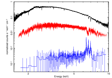
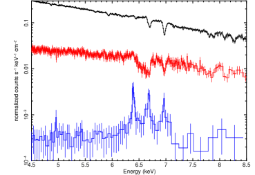
Figure 1.— GRS 1915$+$105 in states reminiscent of Seyfert 1 and Seyfert 2 AGN. The lefthand panel shows the full pass band; the righthand panel focuses on the Fe K region. In black: the spectrum from a steady soft state with a strong disk wind; accretion disk P-Cygni profiles are evident (ObsID 16711; Miller et al. 2016). In red: the spectrum from ObsID 22213 as GRS 1915$+$105 entered the obscured state. The absorption trough between 6.4–6.7 keV indicates a broad range of charge states. In blue: the spectrum from ObsID 22885. The emission lines are many times stronger than the local continuum. The spectrum is likely consistent with the central source being embedded in Compton-thick obscuration. (The spectra were been binned for visual clarity.)

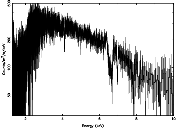
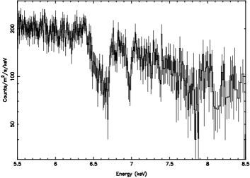
Figure 2.— The spectrum from ObsID 22213, obtained as GRS 1915$+$105 entered the obscured state (also see Figure 1). The data were binned within SPEX according to the “optimal” binning scheme of Kaastra & Bleeker (2016). LEFT: The spectrum over the full pass band; He-like and H-like absorpotion lines form Si, S, Ar, Ca, and Fe are evident; lines from less abundant elements may also be present. The Fe absorption features are particularly strong; the He-$\beta$ and Ly-$\beta$ lines of Fe are also evident. The only emission line is the neutral (or, low-ionization) Fe K$\alpha$ line at 6.40 keV. RIGHT: The same spectrum, in the Fe K band. The broad absorption feature between 6.40–6.70 keV likely indicates that a range of Fe charge states likely contribute to the observed spectrum. Initial fits confirmed that no single zone (e.g., no single ionization parameter) could account for this trough and the H-like line close to 6.97 keV.

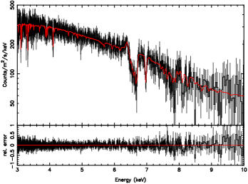
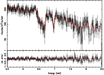
Figure 3.— The spectrum from ObsID 22213, captured as GRS 1915$+$105 entered the obscured state (also see Figure 1). The data were binned according to the “optimal” binning scheme of Kaastra & Bleeker (2016). The model (shown in red) included two layers of photoionized absorption to describe an apparent wind, and reflection with dynamical blurring. The wind is found to be dense, slow-moving, and to originate at small radii. It may not escape from the system, and may build-up the obscuring material that later buries the central engine in a Compton-thick cloud. LEFT: The spectrum and model on a broad pass band. RIGHT: The spectrum and model in the Fe K band. See Table 2 for the spectral fit parameters.

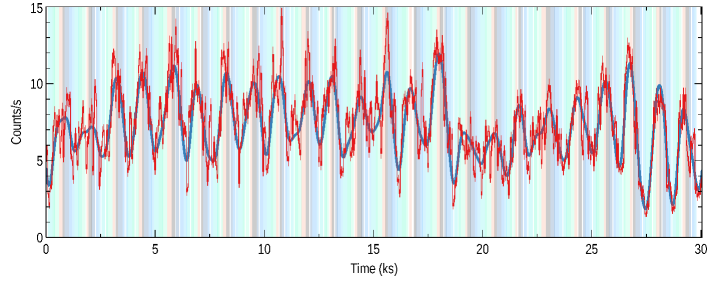
Figure 4.— The light curve of the first-order HEG and MEG events in ObsID 22213, as GRS 1915$+$105 entered the obscured state. The data are shown in red, and the light curve has been binned so that each point represents 50 s of integration. The variations have a quasi-period of approximately P$\simeq$1250 s, and their amplitude approaches $\pm$50%. The blue line is the result of Gaussian Process (GP; Rasmussen et al. 2005) modeling of the light curve (see the text for details). The GP results were used to define oscillation phase bins relative to the crests and troughs, and to then extract spectra from each bin (see Table 2). The oscillation phase bins are indicated by the vertical stripes.

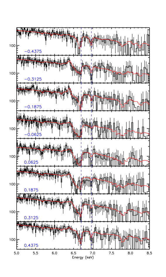
Figure 5.— Phase-selected spectra from ObsID 22213, as GRS 1915$+$105 entered the obscured state. The relative phase of each spectrum is indicated in blue. The phase selections are shown in Figure 4, and the best fit for each phase is detailed in Table 2. Dashed vertical blue lines indicate the rest energy of the He-like Fe XXV (6.70 keV) and H-like Fe XXVI (6.97 keV) resonance absorption lines. The vertical axis in each panel is in units of ${\rm counts}~{}{\rm m}^{-2}~{}{\rm s}^{-1}~{}{\rm keV}^{-1}$. Each phase-selected spectrum has been fit with the same model used to fit the time-averaged spectrum. The best-fit model for each phase-selected spectrum is shown in red. Significant variations are seen in both of the photoionized absorbers and the reflector (again, see Table 2).

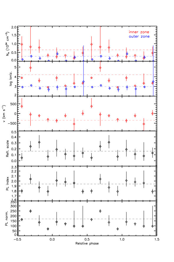
Figure 6.— Critical model parameters versus relative phase, based on spectral fits to phase-selected spectra from ObsID 22213 (see Figures 2–5, and Table 2). Dashed horizontal lines in each panel indicate the best-fit value of the parameter measured in fits to the time-averaged spectrum. The $1\sigma$ errors are plotted. Two cycles are plotted for clarity.

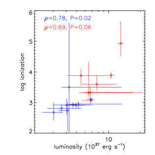
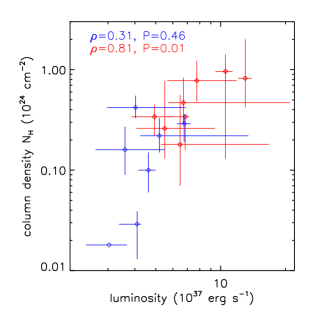
Figure 7.— Inner (red) and outer (blue) photoionized absorber properties versus luminosity, from fits to the “phase-resolved” spectra of ObsID 22213 as GRS 1915$+$105 entered the obscured state (also see Table 2). The Spearman’s rank correlation coefficient, $\rho$, and the probability of false correlation, $P$, are noted for each zone in each panel. The inner zone properties are correlated with luminosity; in contrast, the outer zone parameters are uncorrelated. Note that the outer zone properties are evaluated and plotted versus the “effective” luminosity seen by the zone, after the continuum has passed through the inner zone.

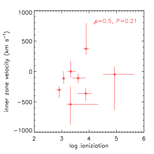
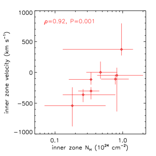
Figure 8.— Additional properties of the inner photoionization zone observed in ObsID 22213, as GRS 1915$+$105 entered the obscured state. Note that negative velocities are blue-shifts. The Spearman’s rank correlation coefficient, $\rho$, and the probability of false correlation, $P$, are noted in each panel. The projected outflow velocity is not significantly correlated with the ionization of the gas, indicating that radiation driving is likely unimportant. However, the outflow velocity is strongly and significantly correlated with the column density of the gas. As the column density of the inner zone increases, the central engine is less able to expel the gas; at the highest observed columns, the gas is red-shifted. This may be an important clue as to the physical mechanisms that created the obscured state in GRS 1915$+$105.

Table 2Fits to ObsID 22213, as GRS 1915$+$105 Entered the Obscured State

Parameter	Time-avg.	One	Two	Three	Four	Five	Six	Seven	Eight
		$\phi=-0.4375$	$\phi=-0.3125$	$\phi=-0.1875$	$\phi=-0.0625$	$\phi=0.0625$	$\phi=0.1875$	$\phi=0.3125$	$\phi=0.4375$
$N_{H,inner}$	$0.7^{+0.1}_{-0.2}$	$1.0^{+0.5}_{-0.8}$	$0.8^{+2.7}_{-0.4}$	$0.8^{+0.5}_{-0.3}$	$0.3^{+0.1}_{-0.1}$	$0.3^{+0.5}_{-0.1}$	$0.34^{+0.01}_{-0.18}$	$0.2^{+0.4}_{-0.1}$	$0.5^{+0.4}_{-0.2}$
log$\xi_{inner}$	$4.2^{+0.1}_{-0.3}$	$3.6^{+0.1}_{-0.1}$	$4.9^{+0.7}_{-0.4}$	$3.6^{+0.3}_{-0.2}$	$2.9^{+0.1}_{-0.1}$	$3.9^{+0.2}_{-0.3}$	$3.07^{+0.05}_{-0.04}$	$3.32^{+1.0}_{-0.1}$	$3.3^{+0.2}_{-0.1}$
$\sigma_{inner}$	$70^{+18}_{-21}$	$70^{*}$	$70^{*}$	$70^{*}$	$70^{*}$	$70^{*}$	$70^{*}$	$70^{*}$	$70^{*}$
$v_{inner}$	$-35^{-70}_{+70}$	$360^{+420}_{-100}$	$-50^{-590}_{+120}$	$-110^{-90}_{+70}$	$-300^{-130}_{+60}$	$-360^{-120}_{+90}$	$-120^{-90}_{+120}$	$-540^{-3340}_{+300}$	$0_{-100}^{+170}$
$N_{H,outer}$	$0.28^{+0.05}_{-0.04}$	$0.08^{+0.08}_{-0.04}$	$0.29^{+0.07}_{-0.10}$	$0.16^{+0.11}_{-0.07}$	$0.018^{+0.05}_{-0.02}$	$0.42^{+0.13}_{-0.09}$	$0.03^{+0.01}_{-0.02}$	$0.2^{+0.1}_{-0.1}$	$0.0^{+0.9}_{-0.0}$
log$\xi_{outer}$	$2.98^{+0.06}_{-0.06}$	$3.08^{+0.08}_{-0.11}$	$3.11^{+0.08}_{-0.15}$	$2.8^{+0.2}_{-0.2}$	$2.7^{+0.3}_{-0.3}$	$2.9^{+0.2}_{-0.1}$	$2.7^{+0.3}_{-0.7}$	$3.0^{+0.1}_{-0.1}$	$5^{+5}_{-5}$
$\sigma_{outer}$	$30^{+10}_{-10}$	$29^{*}$	$29^{*}$	$29^{*}$	$29^{*}$ $29^{*}$	$29^{*}$	$29^{*}$	$29^{*}$
$v_{outer}$	$-50^{-20}_{+40}$	$0^{*}$	$0^{*}$	$0^{*}$	$0^{*}$	$0^{*}$	$0^{*}$	$0^{*}$	$0^{*}$
$\Gamma$	$1.94^{+0.05}_{-0.04}$	$1.74^{+0.04}_{-0.05}$	$2.0^{+0.1}_{-0.1}$	$1.9^{+0.1}_{-0.1}$	$1.8^{+0.1}_{-0.1}$	$2.0^{+0.2}_{-0.1}$	$1.98^{+0.09}_{-0.07}$	$2.0^{+0.3}_{-0.1}$	$1.79^{+0.05}_{-0.05}$
scale	$0.16^{+0.04}_{-0.03}$	$0.05^{+0.08}_{-0.05}$	$0.24^{+0.09}_{-0.08}$	$0.3^{+0.1}_{-0.1}$	$0.1^{+0.1}_{-0.1}$	$0.2^{+0.2}_{-0.1}$	$0.11^{+0.09}_{-0.09}$	$0.1^{+0.2}_{-0.1}$	$0.13^{+0.0}_{-0.08}$
$r_{inner}$	$2200^{+7800}_{-1280}$	$2200^{*}$	$2200^{*}$	$2200^{*}$	$2200^{*}$	$2200^{*}$	$2200^{*}$	$2200^{*}$	$2200^{*}$
cos($\theta$)	$0.95^{+0.01}_{-0.07}$	$0.95^{*}$	$0.95^{*}$	$0.95^{*}$	$0.95^{*}$	$0.95^{*}$	$0.95^{*}$	$0.95^{*}$	$0.95^{*}$
Norm.	$170^{+40}_{-30}$	$140^{+10}_{-20}$	$250^{+20}_{-20}$	$140^{+70}_{-40}$	$70^{+10}_{-20}$	$140^{+90}_{-40}$	$120^{+10}_{-20}$	$100^{+1500}_{-20}$	$100^{+290}_{-10}$
$F_{abs,3-10}$	$1.2^{+0.3}_{-0.2}$	$1.4^{+0.1}_{-0.1}$	$1.26(9)$	$1.1^{+0.6}_{-0.3}$	$0.9(2)$	$0.9^{+0.6}_{-0.3}$	$1.14^{+0.05}_{-0.21}$	$1.3^{+2.0}_{-0.2}$	$1.4^{+4.2}_{-0.2}$
$F_{unabs,0.5-30}$	$11.^{+3}_{-2}$	$11.9^{+0.9}_{-1.3}$	$15(1)$	$9^{+4}_{-2}$	$6(1)$	$6.2^{+4.4}_{-1.6}$	$7.7^{+0.3}_{-1.4}$	$7.3^{+11.7}_{-1.3}$	$7.6^{+22.8}_{-1.2}$
$L_{0.5-30}$	$10^{+3}_{-2}$	$10.6^{+0.8}_{-1.2}$	$13.1(9)$	$8^{+4}_{-2}$	$5(1)$	$5.5^{+3.9}_{-1.4}$	$6.9^{+0.3}_{-1.2}$	$6.5^{+10.4}_{-1.2}$	$6.7^{+20.3}_{-1.0}$
C-stat.	1148.8	424.5	390.9	401.1	439.3	407.0	397.0	386.6	359.9
$\nu$ (dof)	1090	423	378	378	378	378	378	378	378

Table 3Fits to ObsIDs 22885 and 22886, Deep within the Obscured State

Parameter	22885	22885	22886	22886
	(xillver$+$photemis)	(refl$+$pion)	(xillver$+$photemis)	(refl$+$pion)
$N_{H}(10^{24}~{}{\rm cm}^{-2})$	$2.2^{+0.9}_{-0.3}$	0.9(4)	0.35(2)	0.29(4)
$\Gamma$	$2.20_{-0.03}$	–	$2.20_{-0.02}$	–
$\tau$	–	0.65(7)	–	0.6(2)
$K_{continuum}$	$0.7^{+2.0}_{-0.3}$	$0.03^{+0.02}_{-0.01}$	0.12(1)	0.09(2)
$z(10^{-3})$	2.5(5)	–	1.5(6)	–
$f$ or $scale$	$-0.09^{-0.01}_{+0.02}$	$3^{+2}_{-1}$	$-0.14(3)$	$1.7(2)$
$K_{reflection}$	$0.024(2)$	$2(1)$	$0.037(3)$	$5.3(2)$
$N_{H,emis}(10^{24}~{}{\rm cm}^{-2})$	–	$0.12^{+0.15}_{-0.06}$	–	$0.8^{+1.5}_{-0.5}$
log$\xi_{emis}$	$3.40(3)$	$2.6(2)$	$3.50(2)$	$2.7^{+0.2}_{-0.1}$
$z(10^{-3})$	$0.0^{+0.2}$	–	$0.0^{+0.2}$	–
$K_{emis}(10^{2})$	$2.5(3)$	–	$5.8^{+0.6}_{-0.3}$	–
$\Omega$	–	$5^{+4}_{-1}$	–	$0.9^{+1.0}_{-0.5}$
$F_{abs,3-10}$	$3^{+8}_{-1}$	$3^{+2}_{-1}$	$8.8(7)$	$9(2)$
$F_{unabs,0.5-30}$	$3^{+8}_{-1}$	$5^{+3}_{-2}$	$81(7)$	$21(4)$
$L_{0.5-30}$	$3^{+8}_{-1}$	$0.44^{+0.3}_{-0.1}$	$0.72(6)$	$0.19(4)$
$C$-stat	$154.8$	$224.5$	$530.0$	$233.8$
$\nu$ (dof)	140	192	414	187

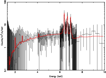
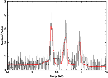
Figure 9.— The combined first-order Chandra/HETG spectrum of GRS 1915$+$105 in ObsID 22885. The spectrum was fit over the broad pass band shown in the lefthand panel; the righthand panel focuses on the crucial Fe K band. Note that the neutral Fe K$\alpha$ line at 6.40 keV, the He-like complex at 6.70 keV, and H-like line at 6.97 keV are all several times stronger than the local continuum. This indicates that most of the ionizing continuum is obscured from direct view. The fits shown here were made in SPEX using a model consisting of line-of-sight absorption, absorption within GRS 1915$+$105 acting on a thermal Comptonizaton and linked, self-consistent photioizonized emission component (via “pion”), and distant neutral reflection without internal obscuration (via “refl”, based on “pexmon”). See Table 3 for best-fit parameter values and errors.

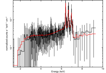
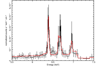
Figure 10.— Similar to Figure 9, but in this figure the spectrum of ObsID 22885 was fit within XSPEC. The model consists of line-of-sight absorption, absorption within GRS 1915$+$105 acting on a cut-off power-law and a photioizonized emission component (via the XSTAR-derived “photemis”), and distant neutral reflection without internal obscuration (via “pexmon”). The spectrum consistent with being Compton-thick (see Table 3). A slightly different binning is used in these fits; please see the text for details.

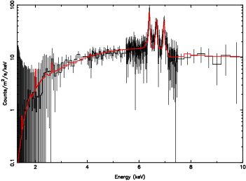
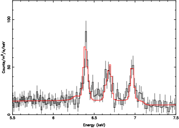
Figure 11.— Similar to Figure 9, but the spectrum from ObsID 22886 and corresponding SPEX model are shown. The best-fit model suggests strong obscuration that is not quite Compton-thick (see Table 3).

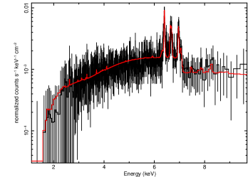
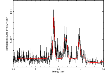
Figure 12.— Similar to Figure 11, but the XSPEC model for ObsID 22886 is shown. This model again suggests strong obscuration that is not quite Compton-thick (see Table 3). This is crudely indicated by the somewhat shallower depth of the Fe K edge in this observation, relative to ObsID 22885 (see Figures 9–10). In this spectrum and with the binning adopted here, the contributions of the He-like triplet components are relatively clear; the strong forbidden line is a clear indication of photoionzation.

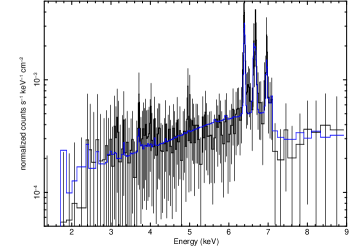
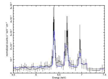
Figure 13.— Fits to ObsID 22885 with an alternative model. The 6.4 keV line is no longer fit with neutral reflection, and the internal obscruation is no longer fit with neutral absorption. Instead, photoionized gas with a low ionization parameter (log$\xi\simeq 1.1$) is used to self-consistently model both the heavy internal obscuration and the 6.40 keV emission line. The absorber has a column density of $N_{H}\simeq 5\times 10^{23}~{}{\rm cm}^{-2}$ and a covering fraction of $f\simeq 0.95$. The He-like and H-like Fe lines are fit with a separate photoionized emission component (log$\xi\simeq 3.4$). The overall fit is not as good as the fit that relied on reflection ($C-stat=199$ versus $C-stat=155$), but the model does not predict a Compton shoulder on the Fe K line and further improvements to the model may make it competitive with the more standard picture. Please see the text for additional details and comments.

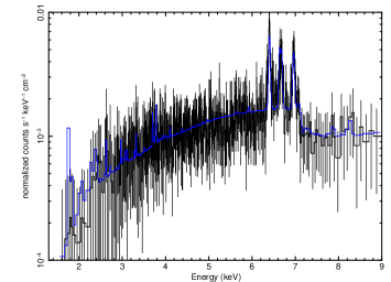
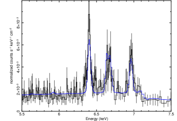
Figure 14.— Similar to Figure 13, but here ObsID 22886 is fit with the alternative model. The coupled low-ionization absorber and re-emitter has a column density of $N_{H}\simeq 5\times 10^{23}~{}{\rm cm}^{-2}$, a covering fraction of $f\simeq 0.95$, and an ionizatin paramter of log$\xi\simeq 1.3$. The more ionized photoionized zone is characterized by log$\xi\simeq 3.5$. The overall fit is not as good as the fit that relied on reflection ($C-stat=580$ versus $C-stat=560$), but the model does not predict a Compton shoulder on the Fe K line and further improvements to the model may make it competitive with the more standard picture. Please see the text for additional details and comments.

References

- (1)
- (2) Arnaud, K., 1996, in ASP Conf. Ser. 101, Astronomical Data Analysis Software Systems V, ed. G. H. Jacoby & J. Barnes (San Francisco, CA: ASP), 17
- (3)
- (4) Balakrishnan, M., Tetarenko, B., Corrales, L., Reynolds, M. T., Miller, J. M., 2019, ATEL 12848
- (5)
- (6) Barret, D., Lam Trong, T., den Herder, J.-W., Piro, L., Cappi, M., et al., 2018, SPIE, 10699, 1
- (7)
- (8) Begelman, M. C., McKee, C. F., Shields, G. A., 1983, ApJ, 221, 70
- (9)
- (10) Blum, J. L., Miller, J. M., Fabian, A. C., Miller, M. C., Homan, J., van der Klis, M., Cackett, E. M., Reis, R. C., 2009, ApJ, 706, 60
- (11)
- (12) Cash, W., 1979, ApJ, 228, 939
- (13)
- (14) Costantini, E., Kaastra, J. S., Arav, N., Kriss, G. A., Steenbrugge, K. C., et al., 2007, A&A, 461, 121
- (15)
- (16) Dannen, R. C., Proga, D., Kallman, T. R., 2019, ApJ, 882, 99
- (17)
- (18) Dere, K. P., Landi, E., Mason, H. E., Monsignori, Fossi, B. C., Young, P. R., 1997, A&AS, 125, 149
- (19)
- (20) Elvis, M., Risaliti, G., Nicastro, F., Miller, J. M., Fiore, F., Puccetti, S., 2004, ApJ, 615, L25
- (21)
- (22) Fender, R. P., Garrington, S. T., McKay, D. J., Muxlow, T., Pooley, G., Spencer, R., Stirling, A., Waltman, E., 1999, MNRAS, 304, 865
- (23)
- (24) Foreman-Mackey, D., Agol, E., Ambikasaran, S., Angus, R., 2017, AJ, 154, 220
- (25)
- (26) Ganguly, S., & Proga, D., 2020, ApJ, 890, 54
- (27)
- (28) Garcia, J., Dauser, T., Lohfink, A., Kallman, T., Steiner, J., McClintock, J., Brenneman, L., Wilms, J., Eikmann, W., Reynolds, C., Tombesi, F., 2014, ApJ, 782, 76
- (29)
- (30) Giustini, M., Miniutti, G., & Saxton, R. D., 2020, A&A, 636, L2
- (31)
- (32) Giustini, M., & Proga, D., 2020, in the Proceedings of the IAU Symposium No. 356, “Nuclear Activity in Galaxies Across Cosmic Time” (Addis Ababa, 7-11 Oct. 2019)
- (33)
- (34) Ishibashi, K., Dewey, D., Huenemoerder, D. P., Testa, P., 2006, ApJ, 644, L117
- (35)
- (36) Kaastra, J., & Bleeker, J. A. M., 2016, A&A, 587, 151
- (37)
- (38) Kaastra, J., Mewe, R., Nieuwenhuijzen, H., 1996, in “UV and X-ray Spectroscopy of Astrophysical and Laboratory Plasmas,” eds. K. Yamashita & T. Watanabe, 411
- (39)
- (40) Kallman, T., & Bautista, M., 2001, ApJS, 133, 221
- (41)
- (42) Kallman, T., Evans, D., Marshall, H., Canizares, C., Longinotti, A., Nowak, M., Schulz, N., 2014, ApJ, 780, 121
- (43)
- (44) Kammoun, E. S., Miller, J. M., Koss, M., Oh, K., Zoghbi, A., et al., 2020, ApJ, subm., arxiv:2007.02616
- (45)
- (46) Kammoun, E. S., Miller, J. M., Zoghbi, A., Oh, K., Koss, M., et al., 2019, ApJ, 877, 102
- (47)
- (48) King, A. L., Miller, J. M., Raymond, J., Reynolds, M. T., Morningstar, W., 2015, ApJ, 813, L37
- (49)
- (50) Koljonen, K. I. I., & Tomsick, J. A., 2020, A&A, 639, 13
- (51)
- (52) Komossa, S., Burwitz, V., Hasinger, G., Predehl, P., Kaastra, J. S., Ikebe, Y., 2003, ApJ, 582, L15
- (53)
- (54) Koss, M. J., Blecha, L., Bernhard, P., Hung, C.-L., Lu, J. R., et al., 2018, NAture, 563, 214
- (55)
- (56) La Massa, S. M., Yaqoob, T., Levenson, N. A., Boorman, P., Heckman, T. M., Gandhi, P., Rigby, J. R., Urry, C. M., Ptak, A. F., 2017, ApJ, 835, 91
- (57)
- (58) Landi, E., Young, P. R., Dere, K. P., Del Zanna, G., Mason, H. E., 2013, ApJ, 763, 86
- (59)
- (60) Lee, J. C., Reynolds, C. S., Remillard, R. A., Schulz, N. S., Blackman, E. G., Fabian, A. C., 2002, ApJ, 567, 1102
- (61)
- (62) Magdziarz, P., & Zdziarski, A. A., 1995, MNRAS, 273, 837
- (63)
- (64) Marconi, A., Risaliti, G., Gilli, R., Hunt, L. K., Maiolino, R., Salvati,M., 2004, MNRAS, 351, 169
- (65)
- (66) Marscher, A. P., Jorstad, S. G., Gomez, J.-L., Aller, M. F., Terasranta, H., Lister, M. L., Stirling, A. M., 2002, Nature, 417, 625
- (67)
- (68) Martini, P., & Weinberg, D. H., 2001, ApJ, 547, 12
- (69)
- (70) Matt, G., Guainazzi, M., & Maiolino, R., 2003, MNRAS, 342, 422
- (71)
- (72) McClintock, J. E., Shafee, R., Narayan, R., Remillard, R. A., Davis, S. W., Li, L.-X., 2006, ApJ, 652, 518
- (73)
- (74) Mehdipour, M., Kaastra, J. S., Kriss, G. A., et al., 2015, A&A, 575, 22
- (75)
- (76) Miller, J. M., Balakrishnan, M., Reynolds, M. T., Trueba, N., Zoghbi, A., Kaastra, J., Kallman, T., Proga, D., 2019, ATEL 12743
- (77)
- (78) Miller, J. M., Balakrishnan, M., Reynolds, M. T., Fabian, A. C., Kaastra, J., Kallman, T., 2019, ATEL 12771
- (79)
- (80) Miller, J. M., Cackett, E., Zogbhi, A., Barret, D., Behar, E., et al., 2018, ApJ, 865, 97
- (81)
- (82) Miller, J. M., Fabian, A. C., Kaastra, J., Kallman, T., King, A. L., Proga, D., Raymond, J., Reynolds, C. S., 2015, ApJ, 814, 87
- (83)
- (84) Miller, J. M., & Homan, J., 2005, ApJ, 618, L107
- (85)
- (86) Miller, J. M., Parker, M. L., Fuerst, F., Bachetti, M., Harrison, F. A., et al., 2013, ApJ, 775, L45
- (87)
- (88) Miller, J. M., Raymond, J., Fabian, A. C., Gallo, E., Kaastra, J., Kallman, T., King, A. L., Proga, D., Reynolds, C., Zoghbi, A., 2016, ApJ, 821, L9
- (89)
- (90) Miller, J. M., Raymond, J., Fabian, A., Steeghs, D., Homan, J., Reynolds, C., van der Klis, M., Wijnands, R., 2006, Nature, 441, 953
- (91)
- (92) Miniutti, G., Saxton, R. D., Giustini, M., Alexander, K. D., Fender, R. P., et al., 2019, Nature, 573, 381
- (93)
- (94) Mirabel, I. F., & Rodriguez, L. F., 1998, Nature, 392, 673
- (95)
- (96) Morrison, R., & McCammon, D., 1983, ApJ, 270, 119
- (97)
- (98) Motta, S. E., Kajaba, J. J. E., Sanchez-Fernandez, C., Beardmore, A. P., Sanna, A., et al., 2017, MNRAS, 471, 1797
- (99)
- (100) Motta, S. E., Marelli, M., Pintore, F., Esposito, P., Salvaterra, R., De Luca, A., Israel, G. L., Tiengo, A., Rodriguz Castillo, G. A., 2020, ApJ, in press, arxiv:2006.05384
- (101)
- (102) Motta, S. E., Williams, D., Fender, R., Titterington, D. G., Perrott, Y., 2019, ATEL 12773
- (103)
- (104) Negoro, H., Tachibana, Y., Kawai, N., Yamaoka, K., Ueda, Y., et al., 2018, ATEL 11828
- (105)
- (106) Neilsen, J., & Lee, J. C., 2009, Nature, 458, 481
- (107)
- (108) Neilsen, J., Remillard, R. A., & Lee, J. C., 2011, ApJ, 737, 69
- (109)
- (110) Porquet, D., & Dubau, J., 2000, A&AS, 143, 495
- (111)
- (112) Pogge, R. W., & Martini, P., 2002, ApJ, 569, 624
- (113)
- (114) Ponti, G., Fender, R., Begelman, M., Dunn, R., Neilsen, J., Coriat, M., 2012, MNRAS, 422, L11
- (115)
- (116) Proga, D., 2003, ApJ, 585, 406
- (117)
- (118) Ramos Almeida, C., & Ricci, C., 2017, NatAs, 1, 679
- (119)
- (120) Rasmussen, C. E., & Williams, C. K. I., 2005, Gaussian Processes for Machine Learning, in Adaptive Computation and Machine Learning, MIT Press, Cambridge MA, USA
- (121)
- (122) Reid, M. J., McClintock, J. E., Steiner, J. F., Steeghs, D., Remillard, R., Dhawan, V., Narayan, R., 2014, ApJ, 796, 2
- (123)
- (124) Remillard, R. A., & McClintock, J. E., 2006, ARA&A, 44, 49
- (125)
- (126) Runnoe, J. C., Cales, S., Ruan, J. J., Eracleous, M., Anderson, S. F., et al., 2016, MNRAS, 455, 1691
- (127)
- (128) Shakura, N. I., & Sunyaev, R. A., 1973, A&A, 24, 337
- (129)
- (130) Shields, G. A., McKee, C. F., Lin, D. N. C., & Begelman, M. C., 1986, ApJ, 306, 90
- (131)
- (132) Steeghs, D., McClintock, J. E., Parsons, S. G., Reid, M. J., Littlefair, S., Dhillon, V. S., 2013, ApJ, 768, 185
- (133)
- (134) Stevens, I. R., & Kallman, T., R., 1990, apJ, 365, 321
- (135)
- (136) Svoboda, J., Guainazzi, M., Merloni, A., 2017, A&A, 603, 127
- (137)
- (138) Tashiro, M., Maejima, H., Toda, K., Kelley, R., Reichental, L., et al., 2018, SPIE, 10699, 22
- (139)
- (140) Trueba, N., Miller, J. M., Kaastra, J., Zoghbi, A., Fabian, A. C., Kallman, T., Proga, D., Raymond, J., 2019, ApJ, 886, 104
- (141)
- (142) Ueda, Y., Yamaoka, K., Remillard, R., 2009, ApJ, 695, 888
- (143)
- (144) Urry, C. M., & Padovani, P., 1995, PASP, 107, 803
- (145)
- (146) Vasudevan, R., & Fabian, A. C., 2009, MNRAS, 392, 1124
- (147)
- (148) Wilkins, D. R., & Fabian, A. C., 2012, MNRAS, 424, 1284
- (149)
- (150) Woods, D. T., Klein, R. I., Castor, J. I., McKee, C. F., Bell, J. B., 1996, ApJ, 461, 767
- (151)
- (152) Zdziarski, A. A., Gierlinski, M., Rao, A. R., Vadawale, S. V., Mikolajewska, J., 2005, MNRAS, 360, 825
- (153)
- (154) Zoghbi, A., Miller, J. M., & Cackett, E., 2019, ApJ, 884, 26
- (155)
- (156) Zoghbi, A., Miller, J. M., King, A. L., Miller, M. C., Proga, D., et al., 2016, ApJ, 833, 165
- (157)