Combining Deep Learning and Optimization for Security-Constrained Optimal Power Flow

Abstract

The security-constrained optimal power flow (SCOPF) is fundamental in power systems and connects the automatic primary response (APR) of synchronized generators with the short-term schedule. Every day, the SCOPF problem is repeatedly solved for various inputs to determine robust schedules given a set of contingencies. Unfortunately, the modeling of APR within the SCOPF problem results in complex large-scale mixed-integer programs, which are hard to solve. To address this challenge, leveraging the wealth of available historical data, this paper proposes a novel approach that combines deep learning and robust optimization techniques. Unlike recent machine-learning applications where the aim is to mitigate the computational burden of exact solvers, the proposed method predicts directly the SCOPF implementable solution. Feasibility is enforced in two steps. First, during training, a Lagrangian dual method penalizes violations of physical and operations constraints, which are iteratively added as necessary to the machine-learning model by a Column-and-Constraint-Generation Algorithm (CCGA). Second, another different CCGA restores feasibility by finding the closest feasible solution to the prediction. Experiments on large test cases show that the method results in significant time reduction for obtaining feasible solutions with an optimality gap below 0.1%.

Nomenclature

This section introduces the main notation. Bold symbols are used for matrices (uppercase) and vectors (lowercase). Additional symbols are either explained in the context or interpretable by applying the following general rules: Symbols with superscript “$j$”, “$k$”, or “$l$” denote new variables, parameters or sets corresponding to the $j$-th, $k$-th, or $l$-th iteration of the associated method. Symbols with superscript “$*$” denote the optimal value of the associated (iterating) variable. Symbols with superscript $``t"$ are associated with the data set for the $t$-th past solve. Dotted symbols are associated with predictors for the corresponding variable.

Sets

$\mathcal{E},\mathcal{E}_{s}$

Feasibility sets for variables associated with the nominal state and contingent state $s$, respectively.

$\mathcal{F}_{s}$

Feasibility set for primary response variables under contingent state $s$.

$\mathcal{C}$, $\mathbb{C}$

Full set and subset of constraints.

$\mathcal{G},\mathcal{L},\mathcal{N}$

Sets of generators, transmission lines and buses, respectively.

$\mathcal{S}$, $\mathbb{S}$

Full set and subset of contingencies, respectively.

$\mathcal{T}$, $\mathbb{T}$

Full set and subset of past solves, respectively.

$\mathbb{U}^{+}$, $\mathbb{U}^{-}$

Subsets of line–contingent state pairs.

$\mathcal{Y}_{s}$

Set of decision variables associated with automatic primary response under contingent state $s$.

Parameters

$\alpha$, $\rho$

Learning rate and Lagragian dual step size.

$\beta,\beta_{1},\beta_{c}$

Parameters for selecting constraints.

$\boldsymbol{\gamma}$

Vector of parameters for primary response.

$\gamma_{i}$

Parameter for primary response of generator $i$.

$\epsilon$

Tolerance for transmission line violation.

$\boldsymbol{\lambda},\lambda_{c}$

Vectors for all Lagrangian multipliers and Lagrangian multipliers for constraint $c$.

$\boldsymbol{\nu},\nu_{c},\tilde{\nu}_{c}$

Vector for violations, violation for constraint $c$, and median violation for $c$ among past solves $\mathcal{T}$.

$\mathbf{A}$, $\mathbf{B}$

Line-bus and Generator-bus incidence matrices.

$\boldsymbol{\omega}$

Vector of weights for deep neural network.

$\mathbf{{d}}$

Vector of nodal net loads.

$\mathbf{e}$

Vector of ones with appropriate dimension.

$\mathbf{\overline{f}}$

Vector of line capacities.

$\mathbf{\underline{g}},\mathbf{\overline{g}}$

Vectors of lower and upper limits for generators.

$\overline{g}_{i}$

Upper limit for generator $i$.

$\mathbf{\hat{g}}$

Vector of capacities for generators.

$\hat{g}_{i}$

Capacity of generator $i$.

${h(\cdot)}$

Piecewise linear generation costs.

$\mathbf{K}_{0}$

Matrix of power transfer distribution factors.

$\mathbf{K}_{1}$

Preprocessed matrix for flow limits.

$\mathbf{k}_{2},\mathbf{k}_{3}$

Preprocessed vectors for flow limits.

$\mathbf{\overline{r}}$

Vector of primary response limits of generators.

$\overline{r}_{i}$

Element of $\mathbf{\overline{r}}$ related to generator $i$, given by $\gamma_{i}\hat{g}_{i}$.

$\mathbf{S}$

Angle-to-flow matrix.

Nominal-state-related decision variables and vectors

$\mathbf{\boldsymbol{\theta}},\mathbf{f},\mathbf{g}$

Phase angles, line flows, and nominal generation.

$g_{i}$

Generation of generator $i$ in nominal state.

Contingent-state-related decision variables and vectors

$\mathbf{\boldsymbol{\theta}}_{s}$

Vector of phase angles under contingent state $s$.

$\boldsymbol{\tau}_{s}^{+},\boldsymbol{\tau}_{s}^{-}$

Vectors of line violation under contingent state $s$.

$\phi$, $s_{\phi}$

Highest line violation and related contingent state.

$\tilde{\phi}$

Median highest line violation among instances $\mathcal{T}$.

$\mathbf{f}_{s}$

Vector for line flows under contingent state $s$.

$\mathbf{g}_{s}$

Vector for generation under contingent state $s$.

$\mathbf{g}_{s}^{{}^{\prime}}$

Provisional vector for $\mathbf{g}_{s}$.

$g_{s,i}$

Generation of generator $i$ under contingent state $s$.

$g_{s,i}^{{}^{\prime}}$

Provisional variable for $g_{s,i}$.

$n_{s}$

Global signal under contingent state $s$.

$\mathbf{x}_{s}$

Binary vector indicating whether generators reached $\mathbf{\overline{g}}$ under contingency state $s$.

$x_{s,i}$

Element of $\mathbf{x}_{s}$ corresponding to generator $i$.

I Introduction

I-A Motivation

Power systems operations require constant equilibrium between nodal loads and generation. At the scale of seconds, this balance is achieved by Automatic Primary Response (APR) mechanisms that govern the synchronized generators. For longer time scales, ranging from a few minutes to hours or even days ahead, this balance is obtained by solving mathematical optimization problems, as independent system operators seek consistent and efficient schedules satisfying complex physical and operational constraints. The need to solve these optimization problems in a timely manner is driving intense research about new models and algorithms, both in industry and academia. In this vein, this work aims at speeding up solution times of security-constrained optimal power flow (SCOPF) problem [1, 2, 3, 4, 5, 6, 7] by combining deep learning and robust optimization methods. The SCOPF is solved by operators every few minutes for different sets of bus loads. The high penetration of renewable sources of energy has increased the frequency of these optimizations. The SCOPF problem considered in this work links the APR to the very short-term schedule. It is also relevant to mention that the SCOPF problem is directly or indirectly present in many other power system applications, including security-constrained unit commitment [8], transmission switching [9], and expansion planning [10]. Thus, a reduction in the computational burden would allow system operators to introduce important modeling improvements to many applications.

I-B Contextualization and Related Work

The SCOPF problem determines a least-cost pre-contingency generator dispatch that allows for feasible points of operation for a set of contingencies, e.g., individual failures of main lines and/or generators. The SCOPF problem may refer to the corrective case [5] where re-scheduling is deemed possible and to the preventive case where no re-dispatch occurs [3, 6, 11], i.e., the system must be able to achieve a feasible steady-state point without a new schedule. A valuable review of the SCOPF problem and solution methods is available in [4]. Interesting discussions about credible contingencies, reserve requirements, security criteria, and regulation for reserves can be found in [2, 6, 12] and the references therein. Without loss of generality, the $N-1$ security criterion for generators is adopted in this paper, i.e., the system must operate under the loss of any single generator.

The SCOPF is a nonlinear and nonconvex problem based on the AC optimal power flow (OPF) equations. Extensive reviews can be found in [13] and [14]. The DC formulation of the SCOPF has been widely used in both academia and industry [2, 3, 6, 7]. Interesting discussions regarding the quality of approximations and relaxations of the OPF problem can be found in [15, 16, 17, 18]. The DC-SCOPF can also be used to improve AC-SCOPF approaches [19]. It is not within the scope of this work to discuss the quality of aforementioned approximations or relaxations to the optimal power flow. Instead, this research offers a new approach that improves current industry practices, which is still strongly based on DC-SCOPF.

The APR of synchronized generators is essential for stability. These generators respond automatically to frequency variations, caused by power imbalances for instance, by adjusting their power outputs until frequency is normalized and the power balance is restored. Unfortunately, the APR deployment, which is bounded by generators limits only, may result in transmission line overloads [6, 20, 11]. Therefore, this work co-optimizes the APR of synchronized generators within the (preventive) SCOPF problem. Even though the APR behavior is nonlinear, linear approximations are used in practice [21]. In [22, 6, 7, 23, 11], the APR is modeled by a single variable representing frequency drop (or power loss) for each contingency state and by a participation factor for each generator.

The DC-SCOPF problem with APR is referred to as the SCOPF problem for conciseness in this paper. It admits an exact extensive formulation (with all variables and constraints for nominal state and contingency states) as a mixed-integer linear program (MILP) [6, 11]. Nevertheless, this formulation is generally very large because the APR constraints require binary variables for each generator and for each contingency state to determine whether generators are producing according to the linear response model or are at their limits [6, 11]. Thus, the number of binary variables increases quadratically with the number of generators, which makes the extensive form of the SCOPF impractical. Better modeling strategies and decomposition schemes are required.

The robust optimization framework has been widely applied in power systems due to its interesting tradeoff between modeling capability and tractability. See [24] for a review of robust optimization applications in power systems. The SCOPF problem can be modeled as a two-stage robust optimization or adaptive robust optimization (ARO) and tackled by two main decomposition methods: Benders decomposition [25] and the column-and-constraint-generation algorithm (CCGA) [26]. Both approaches rely on iterative procedures that solve a master problem and subproblems. The master problem is basically the nominal OPF problem with additional cuts/constraints and variables representing feasibility or optimality information on the subproblems. Whereas Benders decomposition provides dual information about the subproblems through valid cuts restricting the master problem, the CCGA adds primal contraints and variables from the subproblems to the master problem.

Unfortunately, the SCOPF problem is not suitable for a traditional Benders decomposition since the subproblems are nonconvex due to the APR constraints (which feature binary variables). Despite such challenges, inspired by [25], an interesting heuristic method was proposed in [6] but it does not guarantee optimality. In contrast, the CCGA algorithm proposed in [11] is an exact solution method which was used to produce optimal solutions to power network with more than 2,000 buses. Notwithstanding aforementioned contributions, both approaches still require significant computational effort to obtain near-optimal solutions.

Machine learning (ML) approaches have been advocated to address the computational burden associated with the hard and repetitive optimization problems in the power sector, given the large amounts of historical data (i.e., past solutions). Initial attempts date back to the early 1990s, when, for example, artificial neural networks were applied to predict the on/off decisions of generators for an unit commitment problem [27, 28]. More recently, ML was used to identify partial warm-start solutions and/or constraints that can be omitted, and to determine affine subspaces where the optimal solution is likely to lie [29]. Artificial neural network and decision tree regression were also used to learn sets of high-priority lines to consider for transmission switching [30], while the k-nearest neighbors approach was used to select previously optimized topologies directly from data [31]. As for the security and reliability aspects of the network, the security-boundary detection was modeled with a neural network to simplify stability constraints for the optimal power flow [32], while decision trees were applied to determine security boundaries (regions) for controllable variables for a coupled natural gas and electricity system [33]. Machine learning was also applied for identifying the relevant sets of active constraints for the OPF problem [34].

Unlike these applications, where the main purpose of machine learning is to enhance the solver performance by classifying sets, eliminating constraints, and/or by modeling specific parts of the problems, the machine-learning approach in [35] directly predicts the generator dispatch for the OPF by combining deep learning and Lagrangian duality. This approach produces significant computational gains but is not directly applicable to the SCOPF problem which features an impractical number of variables and constraints. This work remedies this limitation.

I-C Contributions

The paper assumes the existence of historical SCOPF data, i.e., pairs of inputs and outputs [34, 29, 30, 31, 35] The proposed approach uses a deep neural network (DNN) to approximate the mapping between loads and optimal generator dispatches. To capture the physical, operational, and APR constraints, the paper applies the Lagrangian dual scheme of [35] that penalizes constraint violations at training time. Moreover, to ensure computational tractability, the training process, labeled as CCGA-DNN, mimics a dedicated CCGA algorithm that iteratively adds new constraints for a few critical contingencies. In these constraints, an approximation for the post-contingency generation is adopted to keep the size of the DNN small. The resulting DNN provides high-quality approximations to the SCOPF in milliseconds and can be used to seed another dedicated CCGA to find the nearest feasible solution to the prediction. The resulting approach may bring two orders of magnitude improvement in efficiency compared to the original CCGA algorithm.

In summary, the contributions can be summarized as follows: i) a novel DNN that maps a load profile onto a high-quality approximation of the SCOPF problem, ii) a new training procedure, the CCGA-DNN, that mimics a CCGA, where the master optimization problem is replaced by a DNN prediction, iii) an approximation for the post-contingency generation which keeps the DNN size small, and iv) an dedicated CCGA algorithm seeded with the DNN evaluation to obtain high-quality feasible solutions fast. Of particular interest is the tight combination of machine learning and optimization proposed by the approach.

I-D Paper Organization

This paper is organized as follows. Section II introduces the SCOPF problem. Section III presents the properties of the SCOPF problem and the CCGA for SCOPF. Section IV introduces the deep learning models in stepwise refinements. Section V describes the CCGA for feasibility recovery. Section VI reports the case studies and the numerical experiments and Section VII concludes the paper.

II The SCOPF Problem

II-A The Power Flow Constraints

The SCOPF formulation uses traditional security-constrained DC power flow constraints over the vectors for generation $\mathbf{g}$, flows $\mathbf{f}$, and phase angles $\mathbf{\boldsymbol{\theta}}$. In matrix notations, these constraints are represented as follows:

$$\mathbf{A}\mathbf{f}+\mathbf{B}\mathbf{g}=\mathbf{{d}}$$ (1)

$$\mathbf{f}=\mathbf{S}\mathbf{\boldsymbol{\theta}}$$ (2)

$$-\mathbf{\overline{f}}\leq\mathbf{f}\leq\mathbf{\overline{f}}$$ (3)

$$\mathbf{\underline{g}}\leq\mathbf{g}\leq\mathbf{\overline{g}}$$ (4)

$$\mathbf{A}\mathbf{f}_{s}+\mathbf{B}\mathbf{g}_{s}=\mathbf{{d}} \forall s\in\mathcal{S}$$ (5)

$$\mathbf{f}_{s}=\mathbf{S}\mathbf{\boldsymbol{\theta}}_{s} \forall s\in\mathcal{S}$$ (6)

$$-\mathbf{\overline{f}}\leq\mathbf{f}_{s}\leq\mathbf{\overline{f}} \forall s\in\mathcal{S}$$ (7)

$$\mathbf{g}_{s}\leq\mathbf{\overline{g}} \forall s\in\mathcal{S}$$ (8)

Equations (1)–(4) model the DC power flow in pre-contingency state and capture the nodal power balance (1), Kirchhoff’s second law (2), transmission line limits (3), and generator limits (4). Analogously, equations (5)–(8) model the power flow for each post-contingency state $s$. The bounds $\mathbf{\overline{g}}$ in (4) and (8) may be different from capacity $\mathbf{\hat{g}}$ due to commitment and/or operational constraints.

II-B Automatic Primary Response

The APR is modeled as in [11, 6, 7]: under contingent state $s$, a global variable $n_{s}$ is used to mimic the level of system response required for adjusting the power imbalance. The APR of generator $i$ under contingency $s$, $g_{s,i}-g_{i}$, is proportional to its capacity $\hat{g}_{i}$ and to the parameter $\gamma_{i}$ associated with the droop coefficient, i.e.,

$$g_{s,i}=\min\{g_{i}+n_{s}\gamma_{i}\,\hat{g}_{i},\;\overline{g}_{i}\} \forall i\in\mathcal{G},\forall s\in\mathcal{S},i\neq s$$ (9)

$$g_{s,s}=0 \forall s\in\mathcal{S}.$$ (10)

These equations are nonconvex and can be linearized by introducing binary variables $x_{s,i}$ to denote whether generator $i$ in scenario $s$ is not at its limit, i.e.,

$$|g_{s,i}-g_{i}-n_{s}\gamma_{i}\hat{g}_{i}|\leq\overline{g}_{i}(1-x_{s,i}) \forall i\in\mathcal{G},s\in\mathcal{S},i\neq s$$ (11)

$$g_{i}+n_{s}\gamma_{i}\,\hat{g}_{i}\geq\overline{g}_{i}(1-x_{s,i}) \forall i\in\mathcal{G},s\in\mathcal{S},i\neq s$$ (12)

$$g_{s,i}\geq\overline{g}_{i}(1-x_{s,i}) \forall i\in\mathcal{G},s\in\mathcal{S},i\neq s$$ (13)

$$n_{s}\in[0,1] \forall s\in\mathcal{S}$$ (14)

$$x_{s,i}\in\{0,1\} \forall i\in\mathcal{G},s\in\mathcal{S}$$ (15)

$$g_{s,s}=0 \forall s\in\mathcal{S}.$$ (16)

II-C Extensive Formulation for the SCOPF Problem

The extensive formulation for the SCOPF problem using variables for generation, flows, and phase angles is as follows:

$$\min_{\mathbf{\boldsymbol{\theta}},\mathbf{f},\mathbf{g},[\mathbf{\boldsymbol{\theta}}_{s},\mathbf{f}_{s},\mathbf{g}_{s},n_{s},\mathbf{x}_{s}]_{s\in\mathcal{S}}}\quad h(\mathbf{g})$$ (17)

s.t.: $$\eqref{eq.Master.EnergyBalance}-\eqref{eq.Master.GenCap}$$ (18)

$$\eqref{eq.Conting.EnergyBalance}-\eqref{disj06} \forall s\in\mathcal{S}.$$ (19)

Using power transfer distribution factors (PTDF), constraints (1)–(8) can be replaced by the following constraints:

$$\mathbf{e}^{\top}\mathbf{g}=\mathbf{e}^{\top}\mathbf{d}$$ (20)

$$|\mathbf{K}_{0}(\mathbf{{d}}-\mathbf{B}\mathbf{g})|\leq\mathbf{\overline{f}}$$ (21)

$$\eqref{eq.Master.GenCap}$$ (22)

$$\mathbf{e}^{\top}\mathbf{g}_{s}=\mathbf{e}^{\top}\mathbf{d} \forall s\in\mathcal{S}$$ (23)

$$|\mathbf{K}_{0}(\mathbf{{d}}-\mathbf{B}\mathbf{g}_{s})|\leq\mathbf{\overline{f}} \forall s\in\mathcal{S}$$ (24)

$$\eqref{eq.Scenario.GenCap} \forall s\in\mathcal{S}$$ (25)

Constraints (20)–(25) that involve the PTDF matrix $\mathbf{K}_{0}$ are from [36]. The total demand balance for the nominal and contingent states are enforced by (20) and (23) respectively. In constraints (21) and (24), the PTDF matrix translates the power injected by each generator at its bus into its contribution to the flow of each line. These constraints also bound the flows from above and below. Observe that $\mathbf{g}$ and $\mathbf{g}_{s}$ are the only variables in this formulation.

For conciseness, denote the power flow constraints (20)–(22) and (23)–(25) by $\mathbf{g}\in\mathcal{E}$ and $\mathbf{g}_{s}\in\mathcal{E}_{s}$ respectively. Similarly, denote the APR constraints (11)–(16) by $\mathcal{Y}_{s}=[\mathbf{g},\mathbf{g}_{s},\mathbf{x}_{s},n_{s}]\in\mathcal{F}_{s}$. The extensive SCOPF formulation then becomes

$$\min_{\mathbf{g},[\mathbf{g}_{s},\mathbf{x}_{s},n_{s}]_{s\in\mathcal{S}}}\quad {h(\mathbf{g})}$$ (26)

s.t.: $$\mathbf{g}\in\mathcal{E}$$ (27)

$$\mathbf{g}_{s}\in\mathcal{E}_{s} \forall s\in\mathcal{S}$$ (28)

$$\mathcal{Y}_{s}\in\mathcal{F}_{s} \forall s\in\mathcal{S}$$ (29)

Note that the number of binary variables above grows quadratically with the number of generators. Hence, solving (26)–(29) becomes impractical for large-scale systems.

III SCOPF Properties and CCGA

This section introduces key properties of the SCOPF problem and summarizes the CCGA proposed in [11]. These properties are necessary for the CCGA and the ML models. The CCGA serves both as a benchmark for evaluation and is used as part of the feasibility recovery scheme proposed in Section V.

Property 1: For $s\in\mathcal{S}$, given values $\mathbf{g}^{*}$ and $n_{s}^{*}$ for $\mathbf{g}$ and $n_{s}$, there exists a unique value $\mathbf{g}^{*}_{s}$ for $\mathbf{g}_{s}$ that can be computed directly using constraints (11)–(16).

Property 2: Consider $s\in\mathcal{S}$ and a value $\mathbf{g}^{*}$ for $\mathbf{g}$. If there exists a value $n_{s}^{*}$ for $n_{s}$ that admits a feasible solution to constraints (11)–(16) and (23), then this value $n_{s}^{*}$ is unique and can be computed by a simple bisection method [11].

Property 2 holds since, for a given $\mathbf{g}^{*}$, each component of $\mathbf{g}_{s}$ is continuous and monotone with respect to $n_{s}$. Hence the value $n_{s}^{*}$ and its associated vector $\mathbf{g}_{s}^{*}$ that satisfy constraint (23) can be found by a simple bisection search over $n_{s}$.

Property 3: Constraint (24) can be formulated as

$$\mathbf{K}_{1}\mathbf{g}_{s}+\mathbf{k}_{2}\geq\mathbf{0}$$ (30)

$$\mathbf{K}_{1}\mathbf{g}_{s}+\mathbf{k}_{3}\geq\mathbf{0},$$ (31)

using matrix operations to obtain $\mathbf{K}_{1}$, $\mathbf{k}_{2}$, and $\mathbf{k}_{3}$.

Note that each row of $\mathbf{K}_{1}$ and each element of $\mathbf{k}_{2}$ and $\mathbf{k}_{3}$ are associated with a specific transmission line. Therefore, for each $s\in\mathcal{S}$ and for each line, the (positive and negative) violation of the thermal limit of the line can be obtained by inspecting (30)–(31) for the proposed value $\mathbf{g}_{s}^{(*)}$.

III-A The Column and Constraint Generation Algorithm

The CCGA, which relies on the above properties, alternates between solving a master problem to obtain a nominal schedule $\mathbf{g}$ and a bisection method to obtain the state variables of each contingency. The master problem is specified as follows:

$$\min_{\mathbf{g},[\mathbf{g}_{s}^{{}^{\prime}}]_{s\in\mathcal{S}},[\mathbf{x}_{s},n_{s}]_{s\in\mathbb{S}}}\quad {h(\mathbf{g})}$$ (32)

s.t.: $$\mathbf{g}\in\mathcal{E}$$ (33)

$$\mathbf{g}_{s}^{{}^{\prime}}-\mathbf{g}\leq\mathbf{\overline{r}} \forall s\in\mathcal{S}$$ (34)

$$\eqref{eq.Scenario.GenCap},\eqref{valid.pstcont},\eqref{disj06} \forall s\in\mathcal{S}$$ (35)

$$\mathcal{Y}_{s}\in\mathcal{F}_{s} \forall s\in\mathbb{S}$$ (36)

$$\mathbf{K}^{l}_{1}\mathbf{g}_{s}^{{}^{\prime}}+\mathbf{k}^{l}_{2}\geq\mathbf{0} \forall(l,s)\in\mathbb{U}^{+}$$ (37)

$$\mathbf{K}^{l}_{1}\mathbf{g}_{s}^{{}^{\prime}}+\mathbf{k}^{l}_{3}\geq\mathbf{0} \forall(l,s)\in\mathbb{U}^{-}$$ (38)

Constraints (32)–(38) uses variables $\mathbf{g}_{s}^{{}^{\prime}}$ to denote a “guess” for the post-contingency generation: the actual vector $\mathbf{g}_{s}$ is not determined by the master problem but by the aforementioned bisection method. Constraint (33) enforces the nominal state constraints. Constraint (34) imposes a valid bound for post-contingency generation. For all contingencies, constraint (35) enforces the generation capacity (8), total demand satisfaction (23), and the absence of generation for a failed generator (16). The APR is enforced “on-demand” in (36) for a reduced set of contingent states $\mathbb{S}$. Initially, $\mathbb{S}=\emptyset$. Inequalities (37)–(38) are also the “on-demand” versions of (30)–(31) for (a few) pairs of transmission lines and contingencies. Initially, $\mathbb{U}^{+}$ and $\mathbb{U}^{-}$ are empty sets.

The CCGA algorithm is specified in Algorithm 1. At iteration $j$, the master problem (32)–(38) computes $\mathbf{g}^{j}$. The bisection method then determines the contingent state variables $[\mathbf{g}_{s}^{j},\mathbf{x}_{s}^{j},n_{s}^{j}]_{s\in\mathcal{S}}$. The vectors $\boldsymbol{\tau}_{s}^{+}$ and $\boldsymbol{\tau}_{s}^{-}$ of positive numbers represent the positive and negative violations of transmission lines for contingent state $s$: they are calculated for all $s\in\mathcal{S}$ by inspecting constraints (30)–(31) for $[\mathbf{g}_{s}^{j}]_{s\in\mathcal{S}}$. The algorithm then computes the highest single line violation $\phi$ among all contingent states and uses $s_{\phi}$ to denote the contingent state associated with $\phi$. The pairs lines/contingencies featuring violations above a predefined threshold $\beta$ are added to the master problem by updating sets $\mathbb{U}^{+}$ and $\mathbb{U}^{-}$. Likewise, $s_{\phi}$ is added to $\mathbb{S}$. As a result, the variables and APR constraints associated with $s_{\phi}$ are added to the master problem during the next iteration. The CCGA terminates when $\phi<\epsilon$, where $\epsilon$ is the tolerance for line violation.

Algorithm 1 CCGA

1:Initialization: $j\leftarrow 0,\mathbb{S}\leftarrow\emptyset$, $\mathbb{U}^{+}\leftarrow\emptyset$, $\,\mathbb{U}^{-}\leftarrow\emptyset$

2:for $j=0,1,\ldots$ do

3:    solve (32)–(36) to obtain $\mathbf{g}^{j}$

4:    $n^{j}_{s}\leftarrow$ apply the bisection method on all $s\in\mathcal{S}$

5:    $\mathbf{g}^{j}_{s}\leftarrow$ enforce (11)–(16) on all $s\in\mathcal{S}$

6:    $\boldsymbol{\tau}_{s}^{-}$, $\boldsymbol{\tau}_{s}^{+}\leftarrow$ get the line violations of $\mathbf{g}_{s}^{j}$ using (30)–(31) for all $s\in\mathcal{S}$

7:    $\phi\leftarrow$ compute the highest line violation among all $s\in\mathcal{S}$

8:    $s_{\phi}\leftarrow$ select the contingent state associated with $\phi$

9:    $\mathbb{S}\leftarrow\mathbb{S}\cup\{s_{\phi}\}$

10:    $\mathbb{U}^{+}\leftarrow\mathbb{U}^{+}\cup\{\,(l,s)\,|\,\boldsymbol{\tau}^{+}_{s}[l]>\beta\}$

11:    $\mathbb{U}^{-}\leftarrow\mathbb{U}^{-}\cup\{\,(l,s)\,|\,\boldsymbol{\tau}^{-}_{s}[l]>\beta\}$

12:    BREAK if $\phi\leq\epsilon$.

13:end for

The following result from [11] ensures the correctness of CCGA: It shows that a solution to the master problem produces a nominal generation for which there exists a solution to each contingency that satisfies the APR and total demand constraints. Since the CCGA adds at least one violated line constraint and, possibly, a set of violated APR constraints for one contingency to the master problem at each iteration, it is guaranteed to converge after a finite number of iterations.

Theorem 1: For each solution $\mathbf{g}^{*}$ to the master problem, there exist values $n^{*}_{s}$ and $\mathbf{g}^{*}_{s}$ that satisfy the demand constraint $\mathbf{e}^{\top}\mathbf{g}^{*}_{s}=\mathbf{e}^{\top}\mathbf{d}$ and the APR constraints (11)–(16) for each contingency $s$.

Proof: By (8) and (34), $g_{s,i}^{{}^{\prime}}\leq\min{\{\overline{g}_{i},g_{i}+\gamma_{i}\hat{g}_{i}\}}$ for each $i$ and $s$, where $g_{s,i}^{{}^{\prime}}$ is the $i$-th element of $\mathbf{g}_{s}^{{}^{\prime}}$. When $n_{s}=0$, $\mathbf{g}_{s}=\mathbf{g}$, except for $g_{s,s}=0$. When $n_{s}=1$, $g_{s,i}=\min{\{\overline{g}_{i},g_{i}+\gamma_{i}\hat{g}_{i}\}}\geq g_{s,i}^{{}^{\prime}}$ for each $i$ and $s$, with $i\neq s$. Since, by (23), $\mathbf{g}_{s}^{{}^{\prime}}$ meets the global demand, $\mathbf{e}^{\top}\mathbf{g}_{s}\geq\mathbf{e}^{\top}\mathbf{g}_{s}^{{}^{\prime}}=\mathbf{e}^{\top}\mathbf{d}$ when $n_{s}=1$. By the monotonicity and continuity of $g_{s,i}$ with respect to $n_{s}$ (for a given $g_{i}$), there is a value $n_{s}^{*}$ whose associated $\mathbf{g}_{s}^{*}$ satisfies the demand constraint in (23) and preserves the APR constraints $\square$.

IV Deep Neural Networks for SCOPF

This section describes the use of supervised learning to obtain DNNs that map a load vector into a solution of the SCOPF problem. A DNN consists of many layers, where the input for each layer is typically the output of the previous layer [37]. This work uses fully-connected DNNs.

IV-A Specification of the Learning Problem

For didactic purposes, the specification of the learning problem uses the extensive formulation (26)–(29). The training data is a collection of instances of the form

$$\{\mathbf{d}^{t};\mathbf{g}^{t},[\mathbf{g}^{t}_{s},n^{t}_{s},\mathbf{x}^{t}_{s}]_{s\in\mathcal{S}}\}_{t\in\mathcal{T}}$$

where $(\mathbf{g}^{t},[\mathbf{g}^{t}_{s},n^{t}_{s},\mathbf{x}^{t}_{s}]_{s\in\mathcal{S}})$ is the optimal solution (ground truth) to the SCOPF problem for input $\mathbf{d}^{t}$. The DNN is a parametric function O$[\boldsymbol{\omega}](\cdot)$ whose parameters are the network $\boldsymbol{\omega}$: It maps a load vector $\mathbf{d}$ into an approximation O$[\boldsymbol{\omega}](\mathbf{d})=\{\mathbf{\dot{g}},[\dot{n}_{s},\mathbf{\dot{x}}_{s},\mathbf{\dot{g}}_{s}]_{s\in\mathcal{S}}\}$ of the optimal solution to the SCOPF problem for load $\mathbf{d}$. The goal of the machine-learning training to find the optimal weights $\boldsymbol{\omega}^{*}$, i.e.,

$$\boldsymbol{\omega}^{*}=\operatorname*{arg\,min}_{\boldsymbol{\omega}} \sum_{t\in\mathcal{T}}\mathbb{L}^{t}_{0}(\mathbf{\dot{g}}^{t})+\sum_{s\in\mathcal{S}}\mathbb{L}^{t}_{s}(\mathbf{\dot{g}}^{t}_{s},\mathbf{\dot{x}}^{t}_{s},\dot{n}^{t}_{s})$$ (39)

s.t.: $$O[\boldsymbol{\omega}](\mathbf{d}^{t})=(\mathbf{\dot{g}}^{t},[\mathbf{\dot{g}}^{t}_{s},\dot{n}^{t}_{s},\mathbf{\dot{x}}^{t}_{s}]) \forall t\in\mathcal{T}$$ (40)

$$\mathbf{\dot{g}}^{t}\in\mathcal{E}^{t} \forall t\in\mathcal{T}$$ (41)

$$\mathbf{\dot{g}}^{t}_{s}\in\mathcal{E}^{t}_{s} \forall t\in\mathcal{T},\forall s\in\mathcal{S}$$ (42)

$$\dot{\mathcal{Y}}^{t}_{s}\in\mathcal{F}^{t}_{s} \forall t\in\mathcal{T},\forall s\in\mathcal{S}$$ (43)

where the loss functions are defined as

$$\mathbb{L}^{t}_{0}(\mathbf{\dot{g}}^{t})=||\mathbf{g}^{t}-\mathbf{\dot{g}}^{t}||_{2}$$

$$\mathbb{L}^{t}_{s}(\mathbf{\dot{g}}^{t}_{s},\mathbf{\dot{x}}^{t}_{s},\dot{n}^{t}_{s})=||\mathbf{g}^{t}_{s}-\mathbf{\dot{g}}^{t}_{s}||_{2}+||\mathbf{x}^{t}_{s}-\mathbf{\dot{x}}^{t}_{s}||_{2}+||n^{t}_{s}-\dot{n}^{t}_{s}||_{2}$$

and minimize the distance between the prediction and the ground truth. There are two difficulties in this learning problem: the large number of scenarios, variables, and constraints, and the satisfaction of constraints (41)–(43). This section examines possible approaches.

IV-B The Baseline Model

The baseline model is a parsimonious approach that disregards constraints (41)–(43) and predicts the nominal generation only, i.e.,

$$\boldsymbol{\omega}^{*}= \operatorname*{arg\,min}_{\boldsymbol{\omega}} \sum_{t\in\mathcal{T}}\mathbb{L}^{t}_{0}(\mathbf{\dot{g}}^{t})$$

s.t.: $$O[\boldsymbol{\omega}](\mathbf{d}^{t})=(\mathbf{\dot{g}}^{t}) \forall t\in\mathcal{T}$$

It uses a DDN model with 5 linear layers, interspersed with 5 nonlinear layers that use the softplus activation function. The sizes of the input and output of each layer are linearly parameterized by $|\mathcal{L}|$ and $|\mathcal{G}|$. A high-level algebraic description of layers of the DNN follows:

$$\mathbf{l}_{i}=\gamma(\mathbf{W}_{i}\mathbf{l}_{i-1}+\mathbf{b}_{i}), \quad\text{for each layer}\;\mathbf{l}_{i}\qquad$$

$$\mathbf{l}_{1}=\gamma(\mathbf{W}_{1}\mathbf{d}+\mathbf{b}_{1})$$

The elements of vector $\boldsymbol{\omega}$ are rearranged as matrices $\mathbf{W}_{i}$ and vector of biases $\mathbf{b}_{i}$. Note that the demand vector $\mathbf{d}$ is the input for the first layer. The symbol $\gamma$ denotes a nonlinear activation function. Unfortunately, training the baseline model tends to produce predictors violating the problem constraints [34, 35].

IV-C A Lagrangian Dual Model for Nominal Constraints

This section extends the baseline model to include constraints on the nominal state (41). Constraints (42)–(43) on the contingency cases are not considered in the model. To capture physical and operational constraints, the training of the DNN adopts the Lagrangian dual approach from [35].

The Lagrangian dual approach relies on the concept of constraint violations. The violations of a constraint $f(x)=0$ is given by $|f(x)|$, while the violations of $f(x)\geq 0$ are specified by $\max(0,-f(x))$. Although these expressions are not differentiable, they admit subgradients. Let $\mathbb{C}$ represent the set of nominal constraints and $\nu_{c}(\mathbf{g})$ be the violations of constraint $c$ for generation dispatch $\mathbf{g}$. The Lagrangian dual approach introduces a term $\lambda_{c}\nu^{t}_{c}(\mathbf{g}^{t})$ in the objective function for each $c\in\mathbb{V}$ and each $t\in\mathcal{T}$, where $\lambda_{c}$ is a Lagrangian multiplier. The optimization problem then becomes

$$LR(\boldsymbol{\lambda})= \min_{\boldsymbol{\omega}} \quad\sum_{t\in\mathcal{T}}(\mathbb{L}^{t}_{0}(\mathbf{\dot{g}}^{t})+\sum_{c\in\mathcal{C}}\lambda_{c}\nu^{t}_{c}(\mathbf{\dot{g}}^{t}))$$ (44)

s.t. $$\quad O[\boldsymbol{\omega}](\mathbf{d}^{t})=(\mathbf{\dot{g}}^{t}) \forall t\in\mathcal{T}$$ (45)

and the Lagrangian dual is simply

$$LD=\max_{\boldsymbol{\lambda}}\ LR(\boldsymbol{\lambda})$$ (46)

Problem (46) is solved by iterating between training for weights $\boldsymbol{\omega}$ and updating the Lagrangian multipliers. Iteration $j$ uses Lagrangian multiplier $\boldsymbol{\lambda}^{j}$ and solves $LR(\boldsymbol{\lambda}^{j})$ to obtain the optimal weights $\boldsymbol{\omega}^{j}$. It then updates the Lagrangian multipliers using the constraint violations. The overall scheme is presented in Algorithm 2. Lines 3–10 train weights $\boldsymbol{\omega}^{j}$ for a fixed vector of Lagrangian multipliers $\boldsymbol{\lambda}^{j}$, using minibatches and a stochastic gradient descent method with learning rate $\alpha$. For each minibatch, the algorithm computes the predictions (line 6), the constraint violations (line 7), and updates the weights (line 9). Lines 2–13 describe the solving of Lagrangian dual. It computes the Lagrangian relaxation described previously and updates the Lagrangian multipliers in line 11 using the median violation $\tilde{\nu}_{c}$ for each nominal constraint $c$.

Algorithm 2 Lagrangian Dual Model ($\mathcal{T}$, $\mathbb{C}$, $\alpha$, $\rho$, Jmax, $\boldsymbol{\lambda}^{0}$, $\boldsymbol{\omega}^{0}$)

1:$j\leftarrow 0$.

2:for $j=0,1,\ldots,{\it Jmax}$ do

3:    for $k=0,1,\ldots$ do

4:        Sample minibatch: $\mathbb{T}_{k}\subset\mathcal{T}$

5:        for $t\in\mathbb{T}_{k}$ do

6:           Compute O$[\boldsymbol{\omega}^{j}](\mathbf{d}^{t})=\mathbf{\dot{g}}^{t}$ and $\mathbb{L}^{t}_{0}(\mathbf{\dot{g}}^{t})$

7:           Compute $\nu^{t}_{c}(\mathbf{\dot{g}}^{t})$ $\forall c\in\mathbb{C}$

8:        end for

9:        $\boldsymbol{\omega}^{j}\leftarrow\boldsymbol{\omega}^{j}-\alpha\nabla_{\boldsymbol{\omega}^{j}}[\sum_{t\in\mathcal{T}}(\mathbb{L}^{t}_{0}(\mathbf{\dot{g}}^{t})+\sum_{c\in\mathcal{C}}\lambda_{c}\nu^{t}_{c}(\mathbf{\dot{g}}^{t}))]$

10:    end for

11:    $\lambda^{j+1}_{c}\leftarrow\lambda^{j}_{c}+\rho\,\tilde{\nu}_{c}\;\forall c\in\boldsymbol{C}$

12:    $\boldsymbol{\omega}^{j+1}\leftarrow\boldsymbol{\omega}^{j}$

13:end for

IV-D CCGA-DNN Model

This section presents the final ML model, the CCGA-DNN, which mimics a CCGA algorithm. In particular, the CCGA-DNN combines the Lagrangian dual model with an outer loop that adds constraints for the contingent states on-demand.

Observe first that a direct Lagrangian dual approach to the SCOPF would require an outer loop to add predictors $[\mathbf{\dot{g}}_{s},\mathbf{\dot{x}}_{s},\dot{n}_{s}]_{s\in\mathcal{S}}$ and constraints (42)–(43) for selected contingency states $s$. Unfortunately, the addition of new predictors structurally modifies the DNN output O$[\boldsymbol{\omega}](\cdot)$ and induces a considerable increase in the DNN size.

The key idea to overcome this difficulty is to mimic the CCGA closely, replacing the master problem with the prediction $O[\boldsymbol{\omega}^{l}](\mathbf{d}^{t})$ at iteration $l$. Moreover, constraints (43) are replaced by constraints of the form

$$\dot{g}^{t}_{s,i}=\max\{0,\min\{\dot{g}^{t}_{i}+\dot{n}^{t}_{s}\gamma_{i}\,\hat{g}_{i}\,,\overline{g}_{i}\}\},$$ (47)

where $\dot{n}^{t}_{s}$ is obtained by the bisection method on the prediction. Again, these constraints are not differentiable but admit subgradients and hence can be dualized in the objective function. The CCGA-DNN is summarized in Algorithm 3. At each iteration $l$, the Lagrangian dual model (Algorithm 2) produces updated weights $\boldsymbol{\omega}^{l}$ and multipliers $\boldsymbol{\lambda}^{l}$ (line 5). The inner loop (lines 6–12) applies the bisection method to find $\dot{n}^{t}_{s}$ for all $t$ and constraints (11)–(16) to obtain $\mathbf{\dot{g}}^{t}_{s}$ (lines 8–9). These values are then used to compute the highest line violation $\phi^{t}$ among all states and the associated contingent state $s_{\phi}^{t}$ (line 10). The inner loop also increases the element of the counter vector $\mathbf{p}$ associated with $s_{\phi}^{t}$ whenever the highest violation for solve $t$ is above tolerance $\epsilon$ (line 11). Then, in the main loop, contingency states with high frequencies of violated lines are identified (line 13) using a threshold $\beta_{1}$. The algorithm is terminated if $\mathbb{S}^{{}^{\prime}}$ is empty and median relative violations for nominal constraints in (41) are within tolerances $\beta_{c}$ (line 14). Otherwise, the set of constraints is updated by adding constraints (30)–(31) and (47) for added contingent states (line 15). The Lagrangian multipliers for added constraints (30)–(31) $\forall s\in\mathbb{S}^{{}^{\prime}}$ are initialized in line 16. Finally, constraints (30)–(31) $\forall s\in\mathbb{S}$ are updated with the median violation $\tilde{\phi}$ for those lines associated with some $\phi^{t}$ (line 17). Note that the process of updating Lagrangian multipliers for (30)–(31) $\forall s\in\mathbb{S}$ is different and much stricter than that for nominal constraints in Algorithm 2.

Algorithm 3 CCGA-DNN ($\mathcal{T}$, $\alpha$, $\rho$, $\beta_{1}$, $\beta_{c}$, $\epsilon$, jMax)

1:$\mathbb{C}\leftarrow\{\eqref{ML.const.set01}\}$, $\mathbb{S}\leftarrow\emptyset$, $\boldsymbol{\lambda}^{0}\leftarrow\boldsymbol{0}$, $\boldsymbol{\omega}^{0}\leftarrow\boldsymbol{0}$

2:Create a counter vector $\mathbf{p}$ of size $|\mathcal{S}|$

3:for $l=1,2,\ldots$ do

4:    $\mathbf{p}\leftarrow\mathbf{0}$

5:    $\boldsymbol{\lambda}^{l}$, $\boldsymbol{\omega}^{l}\leftarrow$ Lagrangian Dual Model($\mathcal{T}$, $\mathbb{C}$, $\alpha$, $\rho$, jMax, $\boldsymbol{\lambda}^{l-1}$,$\boldsymbol{\omega}^{l-1}$)

6:    for $t\in\mathcal{T}$ do

7:        $\mathbf{\dot{g}}^{t}\leftarrow$ O$[\boldsymbol{\omega}^{l}](\mathbf{d}^{t})$

8:        $\dot{n}^{t}_{s}\leftarrow$ bisection method, $\forall s\in\mathcal{S}$

9:        $\mathbf{\dot{g}}^{t}_{s}\leftarrow$ enforce (11)–(16), $\forall s\in\mathcal{S}$

10:        Compute: $\phi^{t}$ and identify $s_{\phi}^{t}$

11:        if $\phi^{t}>\epsilon$ then increase $(s_{\phi}^{t})$-th element of $\mathbf{p}$ by 1

12:    end for

13:    $\mathbb{S}^{{}^{\prime}}\leftarrow\{s\,|\,\mathbf{p}[s]\,/\,|\mathcal{T}|>\beta_{1}$}

14:    BREAK if $\mathbb{S}^{{}^{\prime}}\equiv\emptyset$ and $\tilde{\nu_{c}}\leq\beta_{c},\forall c\in\eqref{ML.const.set01}$.

15:    $\mathbb{C}\leftarrow\mathbb{C}\cup\{\eqref{Cut_01}-\eqref{Cut_02},\eqref{cnt.approx.gs},\,\forall s\in(\mathbb{S}^{{}^{\prime}}\setminus\mathbb{S})\}$

16:    $\lambda^{l}_{\eqref{Cut_01}},\,\lambda^{l}_{\eqref{Cut_02}}\leftarrow 0,\;\forall s\in(\mathbb{S}^{{}^{\prime}}\setminus\mathbb{S})$

17:    $\lambda^{l}_{\eqref{Cut_01}},\,\lambda^{l}_{\eqref{Cut_02}}\mathrel{+}=\rho\,\tilde{\phi},\;\forall s\in\mathbb{S}$

18:end for

V Feasibility Recovery and Optimality Gap

The training step produces a set of weights $\boldsymbol{\omega}^{*}$ and the associated DNN produces, almost instantly, a dispatch prediction $\mathbf{\dot{g}}=O[\boldsymbol{\omega}^{*}](\mathbf{d})$ for an input load vector $\mathbf{d}$. However, the prediction $\mathbf{\dot{g}}$ may violate the nominal and contingency constraints. To restore feasibility, this paper proposes a feasibility-recovery CCGA, denoted by FR-CCGA, that finds the feasible solution closest to $\mathbf{\dot{g}}$. The master problem for FR-CCGA is similar to (32)–(38) but it uses a different objective function, i.e.,

$$\min_{\mathbf{g},[\mathbf{g}_{s}^{{}^{\prime}}]_{s\in\mathcal{S}},[\mathbf{x}_{s},n_{s}]_{s\in\mathbb{S}}}\quad ||\mathbf{\dot{g}}-\mathbf{g}||$$ (48)

s.t.: $$\eqref{const.nom}\text{--}\eqref{Cut_02.ccga} \forall\;\mathcal{S},\,\mathbb{S},\,\mathbb{U}^{+},\,\mathbb{U}^{-}$$ (49)

Note that $\mathbf{\dot{g}}$ is a constant vector in FR-CCGA. While CCGA and FR-CCGA are similar in nature, FR-CCGA is significantly faster because $O[\boldsymbol{\omega}^{*}](\mathbf{d})$ is often close to feasibility.

The FR-CCGA and CCGA can be run in parallel to provide upper and lower bounds to the SCOPF respectively. This may be useful for operators to assess the quality of the prediction and the associated FR-CCGA solution and decide whether to commit to the FR-CCGA solutions or wait until a better solution is found or the optimality gap is sufficiently small.

VI Computational Experiments

VI-A Data

The test cases are based on modified versions of 3 system topologies from [38]. Table I shows the size of a single instance for each topology. For each topology, the training and testing data is given by the inputs and solutions of many instances that are constructed as follows. For each instance, the net demand of each bus has a deterministic component and a random component. The deterministic component varies across instances from 82% of the nominal net load to near-infeasibility values by small increments of 0.002%. The random component is independently and uniformly distributed ranging from -0.5% to 0.5% of the corresponding nominal nodal net load for each bus and instance. Algorithm 1 was applied to solve each instance for a maximum line violation of $\epsilon$ = 0.05 MW and an optimality gap of 0.25%.

TABLE I: Instance Size for the SCOPF Problem (26)–(29) after Presolve

System	$|\mathcal{G}|\;\,$	$|\mathcal{L}|\;\,$	$|\mathcal{N}|\;\,$	Total	Binary	Linear
				Variables	Variables	Constraints
118-IEEE	54	186	118	13,466	2,862	19,137
1354-PEG	260	1,991	1,354	387,026	63,455	513,677
1888-RTE	297	2,531	1,888	467,011	79,032	624,780

VI-B Training Aspects

The training set $\mathcal{T}$ is composed by a random sample containing 70% of the generated instances. Algorithm 3 was applied with $\epsilon$ set to 1 MW, $\beta_{1}$ to 5%, $\beta_{c}$ to $1.5\cdot 10^{-2}$, and $\rho$ to $10^{5}$. The inner loop of Algorithm 2 (lines 4–11) is executed $1.5\cdot 10^{5}$ times with a learning rate $\alpha$ varying from $10^{-4}$ to $10^{-10}$ and Jmax was set to 1. The DNN models were implemented using PyTorch package with Python 3.0. The training was performed using NVidia Tesla V100 GPUs and 2 GHz Intel Cores. Table II presents a training summary. In the following, the baseline model is denoted by $\mathcal{M}_{b}$ and the CCGA-DNN by $\mathcal{M}_{ccga}$. Note that the first iteration of Algorithm 3 returns the weights of the baseline model.

TABLE II: Training Summary for Algorithm 3

System	Iterations	Added Contingency States $\mathbb{S}$ (by generator numbers)
118-IEEE	3	{4}
1354-PEG	3	{23, 65, 74, 112, 126, 163, 222}
1888-RTE	2	{152, 153}

VI-C Prediction Quality

Accurate predictions were obtained for all DNN models and topologies. Figure 1 illustrates how $\mathcal{M}_{ccga}$ can learn complex generator patterns arising in the 1354-PEG system. Table III reports the mean absolute errors for predictions $\dot{\mathbf{g}}^{t}$, segmented by generation range: $\mathcal{M}_{b}$ achieves a slightly better accuracy which is expected since it is the less constrained model.

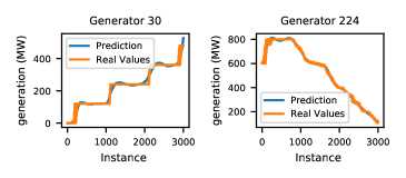
Figure 1: Prediction of $\mathcal{M}_{ccga}$ for selected generators of the 1354-PEG System.

TABLE III: Prediction Mean Absolute Errors (%)

		Generation Range (MW)
System	Model	10	50	100	250	500	1000	2000
		50	100	250	500	1000	2000	5000
118-IEEE	$\mathcal{M}_{b}$	2.3	2.8	0.7	0.3	N/A	N/A	N/A
	$\mathcal{M}_{ccga}$	2.5	3.0	0.7	0.4	N/A	N/A	N/A
1354-PEG	$\mathcal{M}_{b}$	2.4	1.3	1.1	0.9	0.4	0.2	0.1
	$\mathcal{M}_{ccga}$	5.0	1.8	1.2	1.0	0.4	0.3	0.2
1888-RTE	$\mathcal{M}_{b}$	1.3	1.2	0.7	0.4	0.3	0.1	N/A
	$\mathcal{M}_{ccga}$	1.4	1.1	0.6	0.4	0.3	0.1	N/A

Table IV reports selected indicators of violations: the relative violation $\lambda_{\eqref{PTDF_nominal_first}}$ of the total load constraint and the relative violation RLV of the lines associated with $\phi$. The results report median values as well as lower and upper bounds for intervals that capture 95% of the instances. Both models achieve the desired tolerance of $\beta_{c}=1.5\cdot 10^{-2}$ for $\lambda_{\eqref{PTDF_nominal_first}}$ (the tolerance $\beta_{c}$ does not apply to RLV). Model $\mathcal{M}_{ccga}$ produces lower overall violations and has a major effect on RLV.

TABLE IV: Selected Indicators of Violation Across Instances (%)

		$\lambda_{\eqref{PTDF_nominal_first}}$			RLV
System	Model	Median	95%-Interval		Median	95%-Interval
118-IEEE	$\mathcal{M}_{b}$	0.016	0.001	0.055	0.099	0.000	0.467
	$\mathcal{M}_{ccga}$	0.003	0.000	0.011	0.000	0.000	0.548
1354-PEG	$\mathcal{M}_{b}$	0.018	0.001	0.062	0.259	0.086	1.256
	$\mathcal{M}_{ccga}$	0.010	0.000	0.040	0.005	0.000	0.117
1888-RTE	$\mathcal{M}_{b}$	0.012	0.001	0.047	0.205	0.021	1.418
	$\mathcal{M}_{ccga}$	0.005	0.000	0.027	0.007	0.000	0.057
$\lambda_{\eqref{PTDF_nominal_first}}$ – Net load constraint violation divided by total load.
RLV – Relative violation for line associated with $\phi$.

VI-D Comparison with Benchmark CCGA

The previous sections reported on the accuracy of the predictors. This section shows how FR-CCGA leverages the predictors to find near-optimal primal solutions significantly faster than CCGA. More precisely, it compares, in terms of cost and CPU time, CCGA and FR-CCGA when seeded with $\mathcal{M}_{b}$ and $\mathcal{M}_{ccga}$, for $200$ randomly selected instances for each system topology. Each instance was solved with the same tolerances as in the training. They were solved using Gurobi 8.1.1 under JuMP package for Julia 0.6.4 on a laptop Dell XPS 13 9380 featuring a i7-8565U processor at 1.8 GHz and 16 GB of RAM. Tables V, VI, and VII summarize the experiments. Table V reports the distances in percentage between the predictions and the feasible solutions obtained by FR-CCGA when seeded with the predictions. For instance, for $\mathcal{M}_{b}$, this distance is $\sum_{i}|g_{i}^{b}-g_{i}^{f}|/\sum_{i}g_{i}^{f}$, where $g_{i}^{b}$ is $\mathcal{M}_{b}$’s prediction for generator $i$ and $g_{i}^{f}$ is $i$’s generation computed by FR-CCGA seeded with $\boldsymbol{g}^{b}$. As should be clear, the predictions are very close to feasibility. Table VI reports the computation times which show significant increases in performance by FR-CCGA especially when seeded with $\mathcal{M}_{ccga}$ and on the 1354-PEG system, the most challenging network. FR-CCGA is about 160 times faster than CCGA on this test case. FR-CCGA is also significantly more robust when using $\mathcal{M}_{ccga}$ instead of $\mathcal{M}_{b}$. Table VII indicates that the cost/objective increase of FR-CCGA over CCGA is very small for both $\mathcal{M}_{b}$ and $\mathcal{M}_{ccga}$.

TABLE V: Distance between Prediction and Feasible Solution (%)

System	Model	Median	95%-Interval
118-IEEE	$\mathcal{M}_{b}$	0.05	0.01	0.12
	$\mathcal{M}_{ccga}$	0.18	0.05	0.47
1354-PEG	$\mathcal{M}_{b}$	0.05	0.01	0.13
	$\mathcal{M}_{ccga}$	0.09	0.05	0.14
1888-RTE	$\mathcal{M}_{b}$	0.04	0.00	0.10
	$\mathcal{M}_{ccga}$	0.04	0.01	0.07

TABLE VI: CPU Time Comparison

System	Model	Median	Mean	Min.	Max.	Std.
118-IEEE	CCGA	0.210	0.214	0.101	3.717	0.305
	$\mathcal{M}_{b}$	0.024	0.057	0.021	1.580	0.160
	$\mathcal{M}_{ccga}$	0.026	0.068	0.023	1.372	0.171
1354-PEG	CCGA	321.746	327.210	75.585	741.798	127.101
	$\mathcal{M}_{b}$	5.335	8.434	1.320	133.366	13.505
	$\mathcal{M}_{ccga}$	1.521	2.168	0.768	8.449	1.740
1888-RTE	CCGA	5.479	7.406	3.110	30.923	7.073
	$\mathcal{M}_{b}$	5.316	5.501	1.224	18.074	3.348
	$\mathcal{M}_{ccga}$	2.120	1.945	0.911	4.543	0.919

TABLE VII: FR-CCGA Cost Increase over CCGA (%)

System	Model	Median	Mean	Min.	Max.	Std.
118-IEEE	$\mathcal{M}_{b}$	0.021	0.019	-0.073	0.055	0.014
	$\mathcal{M}_{ccga}$	0.027	0.030	-0.010	0.112	0.020
1354-PEG	$\mathcal{M}_{b}$	0.020	0.021	-0.007	0.051	0.012
	$\mathcal{M}_{ccga}$	0.067	0.067	0.032	0.091	0.017
1888-RTE	$\mathcal{M}_{b}$	0.026	0.024	-0.003	0.070	0.011
	$\mathcal{M}_{ccga}$	0.033	0.033	0.004	0.070	0.013

Figure 2 illustrates the behavior of the algorithms on a randomly chosen instance of the 1354-PEG system. The red line represents the upper bound (feasible solution) generated in $1.87$ seconds by the FR-CCGA seeded with $\mathcal{M}_{ccga}$. The blue line represents a sequence of true lower bounds (infeasible solutions) generated by Algorithm 1.

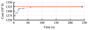
Figure 2: Convergence plot for the $\mathcal{M}_{ccga}$ for the 1354-PEG system.

VII Conclusion

This paper proposed a tractable methodology that combines deep learning models and robust optimization for generating solutions for the SCOPF problem. The considered SCOPF modeled generator contingencies and the automatic primary response of synchronized units. Computational results over two large test cases demonstrate the practical relevance of the methodology as a scalable, easy to specify, and cost-efficient alternative tool for managing short-term scheduling.

References

- [1] O. Alsac and B. Stott, “Optimal load flow with steady-state security,” IEEE Trans. Power App. Syst., vol. PAS-93, no. 3, pp. 745–751, 1974.
- [2] F. Bouffard, F. D. Galiana, and J. M. Arroyo, “Umbrella contingencies in security-constrained optimal power flow,” in 15th Power systems computation conference, PSCC, vol. 5, 2005.
- [3] Y. Li and J. D. McCalley, “Decomposed SCOPF for improving efficiency,” IEEE Trans. Power Syst., vol. 24, no. 1, pp. 494–495, 2009.
- [4] F. Capitanescu, J. M. Ramos, P. Panciatici, D. Kirschen, A. M. Marcolini, L. Platbrood, and L. Wehenkel, “State-of-the-art, challenges, and future trends in security constrained optimal power flow,” Elect. Power Syst. Res., vol. 81, no. 8, pp. 1731–1741, Aug. 2011.
- [5] Q. Wang, J. D. McCalley, T. Zheng, and E. Litvinov, “Solving corrective risk-based security-constrained optimal power flow with lagrangian relaxation and benders decomposition,” Int. J. Elec. Power, vol. 75, pp. 255–264, Feb. 2016.
- [6] Y. Dvorkin, P. Henneaux, D. S. Kirschen, and H. Pandžić, “Optimizing primary response in preventive security-constrained optimal power flow,” IEEE Syst. Journal, vol. 12, no. 1, pp. 414–423, Mar. 2016.
- [7] M. Velay, M. Vinyals, Y. Besanger, and N. Retiere, “Fully distributed security constrained optimal power flow with primary frequency control,” Int. J. Elec. Power, vol. 110, pp. 536–547, Sep. 2019.
- [8] A. Street, F. Oliveira, and J. M. Arroyo, “Contingency-constrained unit commitment with security criterion: A robust optimization approach,” IEEE Trans. Power Syst., vol. 26, no. 3, pp. 1581–1590, 2010.
- [9] A. Khodaei and M. Shahidehpour, “Security-constrained transmission switching with voltage constraints,” Int. J. Electr. Power Energy Syst., vol. 35, no. 1, pp. 74–82, 2012.
- [10] A. Moreira, A. Street, and J. M. Arroyo, “An adjustable robust optimization approach for contingency-constrained transmission expansion planning,” IEEE Trans. Power Syst., vol. 30, no. 4, pp. 2013–2022, 2014.
- [11] A. Velloso, P. Van Hentenryck, and E. S. Johnson, “An exact and scalable problem decomposition for security-constrained optimal power flow,” in Proceedings of the XXI Power Systems Computation Conference (PSCC-2020), 2020.
- [12] Z. Zhou, T. Levin, and G. Conzelmann, “Survey of U.S. ancillary services markets,” Argonne National Lab.(ANL), Argonne, IL (United States), Tech. Rep., 2016.
- [13] L. Platbrood, F. Capitanescu, C. Merckx, H. Crisciu, and L. Wehenkel, “A generic approach for solving nonlinear-discrete security-constrained optimal power flow problems in large-scale systems,” IEEE Trans. Power Syst., vol. 29, no. 3, pp. 1194–1203, 2013.
- [14] F. Capitanescu, “Critical review of recent advances and further developments needed in ac optimal power flow,” Electr. Power Syst. Res., vol. 136, pp. 57–68, 2016.
- [15] F. Li and R. Bo, “Dcopf-based lmp simulation: algorithm, comparison with acopf, and sensitivity,” IEEE Trans. Power Syst., vol. 22, no. 4, pp. 1475–1485, 2007.
- [16] C. Coffrin and P. Van Hentenryck, “A linear-programming approximation of ac power flows,” INFORMS J. Comput., vol. 26, no. 4, pp. 718–734, 2014.
- [17] C. Coffrin, H. L. Hijazi, and P. Van Hentenryck, “The qc relaxation: A theoretical and computational study on optimal power flow,” IEEE Trans. Power Syst., vol. 31, no. 4, pp. 3008–3018, 2015.
- [18] B. Eldridge, R. P. O’Neill, and A. Castillo, “Marginal loss calculations for the dcopf,” Federal Energy Regulatory Commission, Tech. Rep, 2017.
- [19] A. Marano-Marcolini, F. Capitanescu, J. L. Martinez-Ramos, and L. Wehenkel, “Exploiting the use of dc scopf approximation to improve iterative ac scopf algorithms,” IEEE Trans. Power Syst., vol. 27, no. 3, pp. 1459–1466, 2012.
- [20] E. Lannoye, D. Flynn, and M. O’Malley, “Transmission, variable generation, and power system flexibility,” IEEE Trans. Power Syst., vol. 30, no. 1, pp. 57–66, 2014.
- [21] P. Kundur, N. J. Balu, and M. G. Lauby, Power system stability and control. McGraw-hill New York, 1994, vol. 7.
- [22] J. F. Restrepo and F. D. Galiana, “Unit commitment with primary frequency regulation constraints,” IEEE Trans. Power Syst., vol. 20, no. 4, pp. 1836–1842, Nov. 2005.
- [23] K. Karoui, H. Crisciu, and L. Platbrood, “Modeling the primary reserve allocation in preventive and curative security constrained OPF,” in Proc. IEEE PES Trans. Distrb. Conf. Expo. IEEE, Apr., 2010, pp. 1–6.
- [24] X. A. Sun, “Robust optimization in electric power systems,” Advances and Trends in Optimization with Engineering Applications, T. Terlaky, M. F. Anjos, and S. Ahmed, Eds., pp. 357–365, 2017.
- [25] D. Bertsimas, E. Litvinov, X. A. Sun, J. Zhao, and T. Zheng, “Adaptive robust optimization for the security constrained unit commitment problem,” IEEE Trans. Power Syst., vol. 28, no. 1, pp. 52–63, 2013.
- [26] B. Zeng and L. Zhao, “Solving two-stage robust optimization problems using a column-and-constraint generation method,” Oper. Res. Lett., vol. 41, no. 5, pp. 457–461, Sep. 2013.
- [27] H. Sasaki, M. Watanabe, J. Kubokawa, N. Yorino, and R. Yokoyama, “A solution method of unit commitment by artificial neural networks,” IEEE Trans. Power Syst., vol. 7, no. 3, pp. 974–981, 1992.
- [28] Z. Ouyang and S. Shahidehpour, “A hybrid artificial neural network-dynamic programming approach to unit commitment,” IEEE Trans. Power Syst., vol. 7, no. 1, pp. 236–242, 1992.
- [29] A. S. Xavier, F. Qiu, and S. Ahmed, “Learning to solve large-scale security-constrained unit commitment problems,” arXiv preprint arXiv:1902.01697, 2019.
- [30] Z. Yang and S. Oren, “Line selection and algorithm selection for transmission switching by machine learning methods,” in 2019 IEEE Milan PowerTech. IEEE, 2019, pp. 1–6.
- [31] E. S. Johnson, S. Ahmed, S. S. Dey, and J.-P. Watson, “A k-nearest neighbor heuristic for real-time dc optimal transmission switching,” arXiv preprint arXiv:2003.10565, 2020.
- [32] V. J. Gutierrez-Martinez, C. A. Cañizares, C. R. Fuerte-Esquivel, A. Pizano-Martinez, and X. Gu, “Neural-network security-boundary constrained optimal power flow,” IEEE Trans. Power Syst., vol. 26, no. 1, pp. 63–72, 2010.
- [33] D. C. Costa, M. V. Nunes, J. P. Vieira, and U. H. Bezerra, “Decision tree-based security dispatch application in integrated electric power and natural-gas networks,” Electr. Power Syst. Res., vol. 141, pp. 442–449, 2016.
- [34] S. Misra, L. Roald, and Y. Ng, “Learning for constrained optimization: Identifying optimal active constraint sets,” arXiv preprint arXiv:1802.09639, 2018.
- [35] F. Fioretto, T. W. Mak, and P. Van Hentenryck, “Predicting AC Optimal Power Flows: Combining Deep Learning and Lagrangian Dual Methods,” in Thirty-Fourth AAAI Conference on Artificial Intelligence (AAAI-20), 2020.
- [36] A. J. Ardakani and F. Bouffard, “Identification of umbrella constraints in dc-based security-constrained optimal power flow,” IEEE Trans. Power Syst., vol. 28, no. 4, pp. 3924–3934, Nov. 2013.
- [37] Y. LeCun, Y. Bengio, and G. Hinton, “Deep learning,” Nature, vol. 521, no. 7553, pp. 436–444, 2015.
- [38] S. Babaeinejadsarookolaee et al., “The power grid library for benchmarking ac optimal power flow algorithms,” arXiv preprint arXiv:1908.02788, 2019.