Supplementary Materials:
Improving Recognition with
Unlabeled Faces in the Wild

We include some additional experimental details and discussions here that could not be included in the main paper due to space constraints:

• The overview of approaches on improving face recognition (Sec. 1)

• The diversity in datasets (Sec. 2)

• Discussion on the motivation of our choice to model the label noise (Sec. 3)

• The effect of the $\gamma$ hyper-parameter on our proposed uncertainty weighted loss (Sec. 4)

• Details and baselines for overlapping identity separation (Sec. 5)

• Visualization of clustering errors and their correspondence to uncertainty scores (Sec. 6)

• Detailed descriptions of the evaluation benchmarks (Sec. 7)

• Implementation details including training settings for the clustering module and the deep face networks (Sec. 8)

1 Overview

The main submission empirically illustrated the use of unlabeled faces to improve fully-supervised face recognition systems. From the literature, one major direction to boost performance is via supervised training, i.e. , leverage various network structures such as VGG Face [simonyan14very], ResNet [he2016deep] and SE-Net [hu2018squeeze], or investigating effective objective functions, i.e. , triplet loss [schroff2015facenet], Cosine Loss [wang2018cosface], by constraining the feature lying on a hypersphere [liu2017sphereface], or further combine the two [deng2018arcface].

Our paper advocates another direction: leverage larger amounts of unlabeled training data in a semi-supervised manner. These two axes lead to orthogonal developments – more data is likely to improve the next generation of better face architectures and losses. Moreover, tasks such as automatic adaptation of a model to a new scene or condition will benefit from being able to learn from unlabeled faces. There are several use cases for such adaptation: e.g., a particular ethnicity may not have a large labeled dataset but have many unlabeled faces available. In general, deployed models would be able to leverage a continuous stream of unlabeled data to adapt to specific operational conditions.

We briefly re-iterate our main conclusions here – the experiments show that it is indeed possible to further improve the recognition performance of fully-supervised models by exploiting clustering to obtain pseudo-labeled additional data. To see significant improvements, we require comparable volumes of labeled and pseudo-labeled data, as well as accounting for label noise and overlapped identities between labeled and unlabeled sets.

2 On quantifying the diversity in data

In the large-scale uncontrolled setting experiments presented in the main paper, we observe that samples from a different dataset provides greater benefits w.r.t. performance than more samples drawn from the same distribution as the original labeled training dataset. Intuitively this makes sense – different datasets would bring in more information that the original network has not seen earlier during training. We quantify this notion of distance or diversity among datasets using a simple Fréchet distance [dowson1982frechet, heusel2017gans], visualized in Fig. 1. The different datasets are arranged along the x-axis based on distance from labeled MS-Celeb.

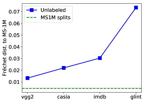
Figure 1: Fréchet distance [dowson1982frechet, heusel2017gans] between MS-1M and the other datasets used as sources of unlabeled data, indicating the domain gap between MS-1M and the unlabeled data.

3 Motivation of Modeling the Label Noise

Here, we begin by discussing some related work regarding our choice of modeling the noisy labels that may motivate our choice of using a linear classifier on top of face descriptor features to decide which cluster assignments are noisy. We note that the label noise from clustering is well-structured, very much unlike the uniform noise (i.e. all categories are equally likely to have their correct label flipped) well-studied in the literature on neural network generalization [zhang2016understanding, arpit2017closer, Forgetting]. Zhang et al. [zhang2016understanding] show that deep neural networks are able to perfectly memorize random labels assigned to the training samples. This would indicate that a network of sufficient expressivity would be able to memorize the incorrect labels in our pseudo-labeled dataset, leading to sub-optimal performance upon re-training with the extra data. Arpit et al. [arpit2017closer] however observe that despite the ability to memorize random patterns, deep neural networks tend to learn easy or correctly-labeled patterns first, and then start fitting to the incorrectly labeled examples in subsequent training epochs. [ICML2019_UnsupervisedLabelNoise] report that the training loss of a network on noisy labeled samples is higher than correctly labeled training samples, and this difference can be used to separate out the noisy labels.

We observe in our initial experiments that at least on our face datasets, the highly-structured labeled noise from clustering assignments behaves differently – even shallower neural networks were learning to fit to both incorrectly and correctly labeled samples at almost concurrent rates, and thus there was no clear separation by looking at the empirical distribution of the training loss. Mixup [zhang2017mixup] shows that encouraging deep neural networks to behaving linearly in between samples improves generalization and tolerance to noise. In fact, [ICML2019_UnsupervisedLabelNoise] report mixup regularization to be useful in their label noise robustness experiments.

Table 1: Effect of tuning hyper-parameter $\gamma$ on the uncertainty weighted loss.

Model	LFW	CFP-fp	IJBA-idt.	IJBA-vrf.
			Rank-1, 5	FAR@1e-3,-4
Baseline GT-1	99.20	92.37	92.66, 96.42	80.23, 69.64
+ GCN	99.48	95.51	94.11, 96.55	87.60, 77.67
+ GCN $\gamma=\frac{1}{3}$	99.60	94.66	94.73, 96.93	87.93, 81.16
+ GCN $\gamma=\frac{1}{2}$	99.45	92.86	93.47, 96.44	84.13, 75.26
+ GCN $\gamma=1$	99.50	94.71	94.76, 97.10	87.97, 79.43
+ GCN $\gamma=2$	99.48	94.71	95.05, 97.26	88.43, 79.87
+ GCN $\gamma=3$	99.55	94.47	94.88, 97.24	88.12, 78.74
+ GT-2 (bound)	99.58	95.56	95.24, 97.24	89.45, 81.02

Our intuition for using linear separability to estimate label noise is as follows – assuming that effective features have been learned by the baseline model on a large labeled dataset, we trust only those cluster assignments that can be fitted by a simple linear classifier on top of these discriminative features. While this does reduce the opportunity of the deep network to learn from some challenging examples (i.e. complicated clusters which are not modeled by a simple linear model would have a high loss that may benefit the network), it also reduces the chance of the high losses from incorrectly-clustered samples from destabilizing the network training.

4 Effect of Hyper-parameter $\gamma$

Setting various values of $\gamma$ in the weighted loss can change the steepness of the weighting curve following a power law:

$$\mathcal{L}^{p}(\mathbf{x}_{i})=(1-p^{-}(\mathbf{x}_{i}))^{\gamma}\mathcal{L}(\mathbf{x}_{i})$$

The behaviour is somewhat like the “focusing parameter” in methods like the focal-loss [lin2017focal]. However, despite some similarities, the motivation and the implementations are starkly different – focal loss seeks to emphasize high-loss samples in a training batch, as a means of hard-example mining; we seek to discount the effect of samples which we suspect are incorrectly pseudo-labeled. Moreover, the focal loss uses the deep network’s softmax output as the posteriors, while we have a separate parametric model to estimate the probability of an incorrect label. We show the re-training performance at different values of $\gamma$ in the uncertainty-weighted loss in Table 1. The parametric Weibull model on the classification-margin appears to be a good estimate of this uncertainty, and changing the shape of the curve gives limited benefits. The focusing parameter is observed to have limited effect in practice – the improvements are not consistent across datasets, and therefore we simply use $\gamma=1$ in all further experiments. We note that other choices than Weibull, e.g.Laplace or beta [ICML2019_UnsupervisedLabelNoise], may be used to parameterize this distribution – our choice was based on the observed skewness of the empirical distribution, which precluded the more common Gaussian.

5 Overlapping Identity Separation

We show the results of modeling the disjoint/overlapping identity separation as an out-of-distribution problem in Table 2. These results were presented in a much condensed form in the main paper. A simple Otsu’s threshold provides acceptably low error rates, i.e., $6.2\%$ false positive rate and $0.69\%$ false negative rate. This shows that our choice of the max-logit score as the feature for OOD is an effective approach.

Table 2: Separating overlapped identities. Results on detecting samples in the unlabeled data whose identity overlaps with classes in the labeled training set.

Method	False Positives	False Negatives	SSE
Naive Otsu	6.2%	0.69%	-
Gaussian-95%	2.01%	0.51%	0.245
Weibull-95%	2.33%	0.50%	0.228

Fig. 2 shows the Weibull and a baseline Gaussian model fit to the empirical distributions of max-logit scores. We quantify the error in fitting the actual data by the sum-of-squared-errors (SSE) between empirical and theoretical PDFs, shown in the last column of Table 2. The Gaussian model has a slighly higher SSE, indicating a worse fit overall. This justifies the decision to fit the maxima using the Weibull family.

Using $95\%$ confidence intervals from Weibulls, we achieve much lower error rates than the simple Otsu’s threshold: ${2.3\%}$ FPR and ${0.50\%}$ FNR. Using Gaussians to threshold the max-logits gives almost equivalent results for overlap separation (slightly better in FP and worse in FN), although the Weibulls fit the skewed distributions better.

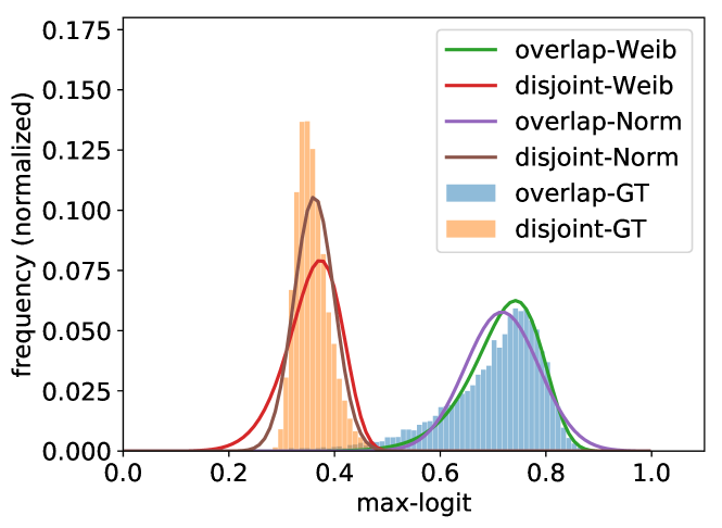
Figure 2: Empirical distribution of the max-logit score for overlapping and disjoint identities between labeled and unlabeled sets (shown on controlled splits of MS-1M dataset). The two-component Weibull and Gaussian models are shown in solid lines.

6 Visualization of Clustering Errors

As discussed in the main paper, our goal is to obtain a model of the noise that can capture the structured label noise resulting from clustering. Re-iterating our steps: (1) train a linear classifier on cluster assignments; (2) define metrics of classification uncertainty such as entropy, classification-margin etc.; (3) to validate the hypothesis, check how well this uncertainty metric corresponds to clustering errors.

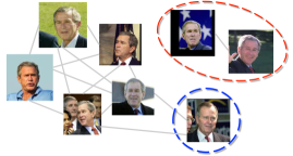
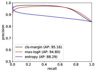
(a)	(b)
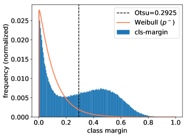
(c)	(d)

Figure 3: Clustering uncertainty. (a) Examples of incorrect pseudo-labels – an image of George Bush Sr. is included in a cluster of George W Bush images (outlier circled in blue); some George W Bush images are spread across multiple clusters (“split ID” circled in red). (b) Precision-recall curves showing Average Precision (AP) of predicting if a cluster assignment is correct using class-margin, max-logit and entropy. (c) Distribution of class-margin with a Weibull fit to the left mode (orange curve). (d) An importance weight is assigned to each pseudo-labeled sample based on its likelihood under the Weibull.

Inliers             Outliers

Figure 4: Cluster outliers. The left column shows inlier samples from 5 clusters. The right column shows faces of different identity being assigned to the same cluster as on the left (outlier samples). The numbers below show the mean and standard deviation of the likelihood of being a noisy label ($p^{-}$). Note that the outlier samples on the right on average have significantly higher likelihood under this noise model. Having a distinctive common attribute like eye-glasses (row 2), facial hair (row 3) or prominent eyebrows (last row) can confound the clustering, even though the identities are different.

True ID             Split-ID

Figure 5: Split-identity clustering. The left column shows samples from 5 clusters. The right column shows faces that share the same identity as on the left, but have been assigned to different clusters. The numbers below show the mean and standard deviation of the likelihood of being a noisy label ($p^{-}$). Note that the “split identity” samples on the right, that have been separated from the “true cluster” of that identity, have higher values under this noise model. E.g. top row: all images belong to the same person (actor Max von Sydow), but due to factors such as age and facial hair, all images are not assigned the same cluster.

To this end, we attempt to quantify the typical errors that occur in cluster assignments (Fig. 3) , based off the standard metrics of precision and recall:

• Outliers: Using ground-truth labels, we first find the modal or most frequent identity in a cluster. Samples corresponding to this identity are inliers. The others are outliers. This type of error affects the precision of the clustering algorithm. Some illustrative examples from the MS-1M splits are shown in Fig. 4, where each row depicts a cluster. The clustering algorithm confuses matching attributes like facial hair, sunglasses, heavy eyebrows etc. for identity, and ends up putting different people into the same cluster.

• Split-identity: This type of error occurs when samples from the same identity as split across different clusters, which impacts the recall metric of a clustering algorithm. For a ground-truth identity, we find all clusters that contain samples belonging to this identity. A perfect clustering would assign all samples of a person to a single cluster, but this is generally not the case – samples of a person can be scattered or split over several clusters . We find the cluster with the highest number of samples for a particular identity, regarding it as the “true cluster”, and the other clusters as having incorrectly split the identity (this is a rough heuristic that we empirically found to be feasible). Some examples of this scenario are shown in Fig. 5. E.g. the first row shows various images of the Swedish actor Max von Sydow. Most of his middle-aged and older images form the largest or “true” cluster, shown on the left. Several images that exhibit other attributes like facial hair or a much younger age end up forming separate clusters, as shown on the right.

As detailed in the main paper, we use precision-recall curves to analyse the correspondence of our uncertainty metrics with clustering errors, finding the highest Average Precision (AP) with classification-margin (95.16%), with max-logits and softmax entropy getting APs of 94.80% and 88.29%, respectively. The empirical distribution of classification-margin scores on a noisy dataset was observed to be bi-modal – incorrect clusterings had a small classification-margin since they were difficult for the logistic regression classifier to learn correctly. In Fig. 3(b), a Weibull distribution fit to the lower mode gives our noise model $p^{-}(\mathbf{x}_{i})$, i.e. the likelihood that a sample $\mathbf{x}_{i}$ has been clustered incorrectly. Figures 4 and 5 also show the average values of $p^{-}(\mathbf{x}_{i})$ for the samples – inliers and true-clusters are typically given a lower likelihood under this model, i.e. we are less uncertain about their cluster assignment.

7 Evaluation Benchmarks

The main paper presents results on the following benchmarks, which we describe in more details here:

• Labeled Faces in the Wild (LFW) [huang2008labeled, learned2016labeled]: consists of 13,233 images and 5749 people, reporting verification accuracy across 10 folds of 300 matching and 300 non-matching face pairs.

• Celebrity Frontal to Profile (CFP) [sengupta2016frontal]: consists of 500 people, each with 10 frontal and 4 profile images. There are two verification protocols – frontal to frontal (ff) and frontal to profile (fp) images. Each protocol consists of 10 folds with 350 same-identity and mismatched-identity pairs.

• IJB-A [klare2015pushing]: part of the challenging IARPA Janus benchmark, it has 500 subjects with 5,397 images and 2,042 videos. Identification performance is reported as retrieval rate at ranks 1 and 5, using 10 splits each with 112 gallery templates and 1763 probe templates (i.e. 1,187 genuine queries and 576 impostor queries whose identities are not in the gallery). Verification performance is reported as True Accept Rate (TAR) at False Accept Rates (FAR) ranging from 1e-1 to 1e-4, evaluated on 10 splits with 11,748 pairs of templates (1,756 positive and 9,992 negative pairs); we report performance at the two most strict settings: FAR@1e-3,1e-4 respectively.

8 Implementation Details

Face recognition training. The CosFace model [wang2018cosface] is used as our face recognition engine, which is one of the top performance methods on standard face recognition benchmarks. A 118-layer ResNet is used as the backbone network. The baseline model on labeled data is trained for 30 epochs using SGD with momentum $0.95$, with a batch size of 512 across 8 GPUs in parallel, starting from a learning rate of 0.1, with the learning rate dropping by a factor of $1/10$ at the $16^{th}$ and $23^{rd}$ epochs. When used as a feature extractor, this model yields vectors of 512 dimensions. When training with pseudo-labeled data, we re-train the entire model from scratch on the union of the labeled and pseudo-labeled data, with the same training settings.

Clustering model training. The Face-GCN implementation uses the publicly available code  of GCN-D from [yang2019learning]. An initial k-nearest neighbor graph is formed over the unlabeled samples with $k=80$, using the FAISS library for efficient similarity computation over large sample sizes. Cluster proposals are generated from this by setting various thresholds – we find optimal settings on a held-out set of MS-Celeb-1M and continue to use these consistently on all the other datasets. The GCN-D model from Face-GCN is trained to predict the precision and/or recall for each cluster proposal. We use a simple 3-layer architecture, with feature sizes: $512\rightarrow 256\rightarrow 64$, following by a global max-pooling. Following [yang2019learning], the model is trained with a regression loss.

Re-training on pseudo-labels. Following the final clustering output from Face-GCN, we discard clusters with fewer than 10 samples as a simple heuristic. The remaining cluster assignments on the remaining samples are treated as category labels and merged with the labeled training set. To control for different optimization settings and validation sets, we simply re-train the face recognition model, from scratch, with the same number of epochs and learning rate schedule as the baseline model trained on labeled data – therefore, the only change between the baseline model and the re-trained model is the extra pseudo-labeled training data.