Chaos in a $Q\bar{Q}$ system at finite temperature and baryon density

Abstract

Onset of chaos for the holographic dual of a $Q\bar{Q}$ system at finite temperature and baryon density is studied. We consider a string in the AdS Reissner-Nordstrom background near the black-hole horizon, and investigate small time-dependent perturbations of the static configurations. The proximity to the horizon induces chaos, which is softened increasing the chemical potential. A background geometry including the effect of a dilaton is also examined. The Maldacena, Shenker and Stanford bound on the Lyapunov exponents characterizing the perturbations is satisfied for finite baryon chemical potential and when the dilaton is included in the metric.

I Introduction

It has been recently conjectured under general assumptions that, for a thermal quantum system at temperature $T$, some out-of-time-ordered correlation functions involving Hermitian operators, for determined time intervals, have an exponential time dependence characterized by an exponent $\lambda$, and that such exponent obeys the bound

$$\lambda\leq 2\pi T$$ (1)

(in units in which $\hbar=1$ and $k_{B}=1$). The correlation functions are related to the thermal expectation values of the (square) commutator of two Hermitian operators at a time separation $t$, which quantify the effect of one operator on later measurements of the other one, a framework for introducing chaos for a quantum system. The conjectured bound, proposed by Maldacena, Shenker and Stanford Maldacena et al. (2016), is remarkable due to its generality. It has been inspired by the observation that black holes (BH) are the fastest ‘scramblers” in nature: the time needed for a system near a BH horizon to loose information depends logarithmically on the number of degrees of freedom of the system Sekino and Susskind (2008); Susskind (2011). The consequences on the connection between chaotic quantum systems and gravity have been soon investigated Shenker and Stanford (2014, 2015); Kitaev (2014); Polchinski (2015). A relation between the size of operators on the boundary quantum theory, involved in the temporal evolution of a perturbation, and the momentum of a particle falling in the bulk has been proposed in a holographic framework Susskind (2018); Brown et al. (2018).

A generalization of the bound (1) for a thermal quantum system with a global symmetry has been proposed Halder (2019):

$$\lambda\leq\frac{2\pi T}{1-\big{|}\frac{\mu}{\mu_{c}}\big{|}},$$ (2)

where $\mu$ is the chemical potential related to the global symmetry, and $\mu_{c}$ is a critical value above which the thermodynamical ensemble is not defined. The inequality (2) is conjectured for $\mu\ll\mu_{c}$ and relaxes the bound (1). Our purpose is to test this generalization.

Several analyses have been devoted to check Eq. (1) using the AdS/CFT correspondence Maldacena (1998); Witten (1998); Gubser et al. (1998), adopting a dual geometry with a black hole, identifying $T$ with the Hawking temperature, for example in de Boer et al. (2018); Dalui et al. (2019). In particular, the heavy quark-antiquark pair, described holographically by a string hanging in the bulk with end points on the boundary Avramis et al. (2007, 2008); Arias and Silva (2010); Nunez et al. (2010), has been studied in this context Hashimoto et al. (2018); Ishii et al. (2017); Akutagawa et al. (2019). For this system $\lambda$ is the Lyapunov exponent characterizing the chaotic behavior of time-dependent fluctuations around the static configuration.

To test the generalized bound (2) one has to include the chemical potential in the holographic description. In QCD, a $U(1)$ global symmetry is connected to the conservation of the baryon number. A dual metric has been identified with the AdS Reissner-Nordstrom (RN) metric for a charged black hole. We can use such a background for testing Eq. (2).

The discussion of the $5d$ AdS-RN metric as a dual geometry for a thermal system with conserved baryon number can be found, e.g., in Lee et al. (2009); Colangelo et al. (2011). The metric is defined by the line element

$$ds^{2}=-r^{2}f\left(r\right)dt^{2}+r^{2}d{\bar{x}}^{2}+\frac{1}{r^{2}f\left(r\right)}dr^{2},$$ (3)

with $r$ the radial bulk coordinate and

$$f\left(r\right)=1-\frac{r_{H}^{4}}{r^{4}}-\frac{\mu^{2}r_{H}^{2}}{r^{4}}+\frac{\mu^{2}r_{H}^{4}}{r^{6}}.$$ (4)

The geometry has an outer horizon located at $r=r_{H}$, and the Hawking temperature is

$$T_{H}=\frac{r_{H}}{\pi}\left(1-\frac{\mu^{2}}{2r_{H}^{2}}\right)\,.$$ (5)

The constant $\mu\leq{\sqrt{2}}\,r_{H}$ in (4) is interpreted as the baryon chemical potential of the boundary theory, and is holographically related to the charge $\hat{Q}$ of the RN black hole: $\hat{Q}=\mu^{2}/r_{H}^{2}$.

The gravity dual of the heavy quark $Q\bar{Q}$ system at finite temperature and chemical potential is a string in the background (3),(4) with the endpoints on the boundary (Fig. 1). To investigate the onset of chaos for this system focusing on the effects of the chemical potential, we use the same approach adopted in Hashimoto et al. (2018) for the system at $\mu=0$, to shed light on the differences with respect to the case of vanishing chemical potential.

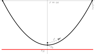
Figure 1: Profile of the static string for the $Q\bar{Q}$ system. $r_{0}$ is the position of the tip of the string, $r_{H}$ the position of the horizon, $L$ the distance between the end points on the boundary.

II Generalities of the suspended string in a gravity background

The AdS-RN metric in (3) belongs to a general class of geometries described by the line element

$$ds^{2}=-g_{tt}(r)dt^{2}+g_{xx}(r)d{\bar{x}}^{2}+g_{rr}(r)dr^{2}\,\,.$$ (6)

The dynamics of a string in such a background is governed by the Nambu-Goto (NG) action

$$S=-\frac{1}{2\pi\alpha^{\prime}}\int\mathrm{d}\tau\mathrm{d}\sigma\sqrt{\det\Big{(}g_{MN}\partial_{a}X^{M}\partial_{b}X^{N}\Big{)}},\;\;\;$$ (7)

with $a,b=(\tau,\sigma)$ and $\alpha^{\prime}$ the string tension. $g_{MN}$ is the metric tensor in (6), $X^{M}$ are the $5d$ coordinates and the derivatives are with respect to the world sheet coordinates $\tau$ and $\sigma$.

We denote by $r_{0}$ the position of the tip of the string as shown in Fig. 1, and $l$ the proper distance measured along the string starting from $r_{0}$. Choosing $\tau=t$ and $\sigma=l$ ($l$-gauge), for a static string laying in the $x-r$ plane with $X^{M}=\left(t,x(l),0,0,r(l)\right)$ the Nambu-Goto action reads:

$$S=-\frac{\mathcal{T}}{2\pi\alpha^{\prime}}\int_{-\infty}^{\infty}\mathrm{d}l\sqrt{F^{2}\left(r\right)\acute{x}^{2}\left(l\right)+G^{2}\left(r\right)\acute{r}^{2}\left(l\right)},$$ (8)

where $\acute{x}=\frac{\partial x}{\partial l}$ and $\acute{r}=\frac{\partial r}{\partial l}$, $F^{2}\left(r\right)=g_{tt}\left(r\right)g_{xx}\left(r\right)$ and $G^{2}\left(r\right)=g_{tt}\left(r\right)g_{rr}\left(r\right)$. For the metric (3) one has $F^{2}(r)=r^{4}f(r)$ and $G(r)=1$.

Note that $x$ is a cyclic coordinate, hence:

$$\acute{x}\left(l\right)=\pm\frac{\acute{r}\left(l\right)}{\sqrt{\frac{r^{4}f\left(r\right)}{r_{0}^{4}f\left(r_{0}\right)}\left(r^{4}f\left(r\right)-r_{0}^{4}f\left(r_{0}\right)\right)}}.$$ (9)

The solution of Eq. (9) is obtained considering that

$$\mathrm{d}l^{2}=g_{xx}\left(r\right)\mathrm{d}x^{2}+g_{rr}\left(r\right)\mathrm{d}r^{2}.$$ (10)

For the unit vector $t^{M}=\left(0,\acute{x}\left(l\right),0,0,\acute{r}\left(l\right)\right)$ tangent to the string at the point with coordinate $l$ the relation holds:

$$g_{MN}t^{M}t^{N} =g_{xx}\left(r\right)\acute{x}^{2}\left(l\right)+g_{rr}\left(r\right)\acute{r}^{2}\left(l\right)$$ (11)

$$=r^{2}\acute{x}^{2}\left(l\right)+\frac{1}{r^{2}f\left(r\right)}\acute{r}^{2}\left(l\right)=1.$$

Including this constraint in Eq. (9) gives

$$\acute{r} = \pm\frac{\sqrt{r^{4}f\left(r\right)-r_{0}^{4}f\left(r_{0}\right)}}{r}$$ (12)

$$\acute{x} = \pm\frac{\sqrt{r_{0}^{4}f\left(r_{0}\right)}}{r^{3}\sqrt{f\left(r\right)}}.$$ (13)

The function $r\left(l\right)$ for the static string can be computed integrating Eq. (12).

The dependence of $L$, the distance between the string endpoints on the boundary, on $r_{0}$ is obtained:

$$L(r_{0})=2\int_{r_{0}}^{\infty}dr\,\frac{r_{0}^{2}\sqrt{f(r_{0})}}{r^{2}\sqrt{f(r)}\sqrt{r^{4}f(r)-r_{0}^{4}f(r_{0})}}\,.$$ (14)

The energy of the string configuration

$$E(r_{0})=\frac{1}{\pi\alpha^{\prime}}\int_{r_{0}}^{\infty}dr\,\frac{r^{2}\sqrt{f(r)}}{\sqrt{r^{4}f(r)-r_{0}^{4}f(r_{0})}}\,\,$$ (15)

diverges and needs to be regularized. A possible prescription is to subtract the bare quark masses, interpreted as the energy of the string consisting in two straight lines from the boundary to the horizon,

$$m_{Q}=\frac{1}{2\pi\alpha^{\prime}}\int_{r_{H}}^{\infty}dr\,\,,$$ (16)

obtaining

$$E_{Q{\bar{Q}}}(r_{0})=$$

$$\frac{1}{\pi\alpha^{\prime}}\left(\int_{r_{0}}^{\infty}dr\,\frac{r^{2}\sqrt{f(r)}}{\sqrt{r^{4}f(r)-r_{0}^{4}f(r_{0})}}-\int_{r_{H}}^{\infty}dr\right)\,.$$

The function $E_{Q{\bar{Q}}}$ can be expressed vs $L$. For the metric in Eq. (4), the distance $L(r_{0})$ has a maximum $L_{max}$, and all values $L\in[0,\,L_{max}]$ are obtained for two positions $r_{0}$. Also the function $E_{Q{\bar{Q}}}(r_{0})$ has a maximum, which decreases and is reached earlier as $\mu$ increases. For each value of the chemical potential there is a value of $r_{0}$ above which there is one energy value indicating a stable string configuration. Below such $r_{0}$, as shown in Fig. 2, the $E_{Q\bar{Q}}(L)$ is not single valued: for each $L$ there are profiles identified by different $r_{0}$, with different energies, corresponding to stable and unstable configurations.

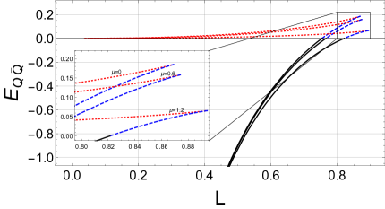
Figure 2: Double valued $E_{Q{\bar{Q}}}(L)$ for $r_{H}=1$ and $\mu=0,\,0.6,\,1.2$. The inset is an enlargement of the $L\simeq 0.8$ range.

III Square string

As suggested in Hashimoto et al. (2018), a simple model suitable for an analytical treatment of the time-dependent perturbations is a square string in the AdS-RN background geometry (3), depicted in Fig. 3.

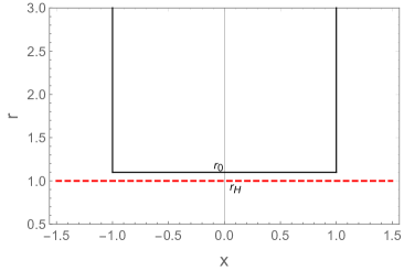
Figure 3: Square string near the horizon, with $r_{H}=1$, $r_{0}=1.1$ and $L=2$.

The model describes quite well a string near the horizon, as shown in Fig. 4 where the profile of the string approaching the horizon is drawn.

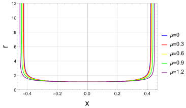
Figure 4: String profile for $r_{H}=1$, $r_{0}=1.1$ and different values of the chemical potential $\mu$.

It is convenient to work in the $r$-gauge ($\tau=t$ and $\sigma=r$). The embedding functions for a string in the $x-r$ plane are $X^{M}=\left(t,x\left(t,r\right),0,0,r\right)$, and the NG action reads

$$S=-\frac{1}{2\pi\alpha^{\prime}}\int\mathrm{d}t\mathrm{d}r\sqrt{1+\acute{x}^{2}\left(r^{4}f\left(r\right)-\frac{1}{f\left(r\right)}\dot{r}^{2}\right)}.$$

(18)

For a static string $X^{M}=\left(t,x\left(r\right),0,0,r\right)$ this reduces to

$$S=-\frac{\mathcal{T}}{2\pi\alpha^{\prime}}\int\mathrm{d}r\sqrt{r^{4}f\left(r\right)\acute{x}^{2}+1}\,\,.$$ (19)

In the case of the square profile, Eq. (19) is determined integrating along the three sides of the string. The result can be regularized as follows:

$$S^{reg}=-\frac{\mathcal{T}}{2\pi\alpha^{\prime}}\left(Lr_{0}^{2}\sqrt{f\left(r_{0}\right)}-2\left(r_{0}-r_{H}\right)\right)\,\,,$$ (20)

where $L$ still denotes the distance between the endpoints on the boundary. For $r_{0}$ near the horizon the energy

$$E=-\frac{S^{reg}}{\mathcal{T}}$$ (21)

has a local maximum, hence upon small perturbations the string departs toward an equilibrium configuration. The stationary point for $E$ is determined solving

$$2Lr_{0}\sqrt{f\left(r_{0}\right)}+\frac{r_{0}^{2}L}{2\sqrt{f\left(r_{0}\right)}}\frac{\partial f\left(r_{0}\right)}{\partial r_{0}}-2=0.$$ (22)

For the metric function $f(r)$ in (4), expanding the lhs of Eq. (22) for $r_{0}\to r_{H}$ gives:

$$r_{0,sol}=\frac{r_{H}\left(L^{2}\left(2r_{H}^{2}+11\mu^{2}\right)-8\right)}{2L^{2}\left(2r_{H}^{2}+5\mu^{2}\right)-8}.$$ (23)

Moreover, expanding for $L\to 0$ at ${\cal O}(L^{2})$ gives

$$r_{0,sol}=r_{H}\left(1+\frac{L^{2}}{8}\left(2r_{H}^{2}-\mu^{2}\right)\right).$$ (24)

We now consider a fluctuating string described by the action in (18), and introduce a small time-dependent perturbation $\delta r\left(t\right)$ to the static solution, $r_{0}\left(t\right)=r_{0,sol}+\delta r\left(t\right)$: indeed, for the square string a perturbation makes time-dependent the position $r_{0}$ of the bottom side. The regularized action is given by

$$S^{reg} = -\frac{1}{2\pi\alpha^{\prime}}\int dt\Bigg{\{}L\sqrt{r_{0}^{4}f\left(r_{0}\right)-\frac{1}{f\left(r_{0}\right)}\dot{r_{0}}^{2}}$$ (25)

$$- 2\left(r_{0}-r_{H}\right)\Bigg{\}}\,\,.$$

The Lagrangian

$$\mathcal{L}=L\sqrt{r_{0}^{4}f\left(r_{0}\right)-\frac{1}{f\left(r_{0}\right)}\dot{r}_{0}^{2}}-2\left(r_{0}-r_{H}\right)$$

(26)

can be expanded around $r_{0,sol}$ to second order in $\delta r(t)$:

$$\mathcal{L}\approx -2r_{0,sol}+2r_{H}+L\,r_{0,sol}^{2}\sqrt{f\left(r_{0,sol}\right)}+\delta r(t)\left(-2+2Lr_{0,sol}\sqrt{f(r_{0,sol})}+\frac{Lr_{0,sol}^{2}f^{\prime}(r_{0,sol})}{2\sqrt{f(r_{0,sol})}}\right)$$ (27)

$$+L\,\delta r(t)^{2}\Bigg{(}\sqrt{f(r_{0,sol})}+\frac{r_{0,sol}f^{\prime}(r_{0,sol})}{\sqrt{f(r_{0,sol})}}-\frac{r_{0,sol}^{2}f^{\prime}(r_{0,sol})^{2}}{8f(r_{0,sol})^{3/2}}+\frac{r_{0,sol}^{2}f^{\prime\prime}(r_{0,sol})}{4\sqrt{f(r_{0,sol})}}\Bigg{)}$$

$$-\delta\dot{r}(t)^{2}\frac{L}{2r_{0,sol}^{2}f(r_{0,sol})^{3/2}},$$

and the equation of motion for $\delta r\left(t\right)$ reads:

$$\delta\ddot{r}(t)\frac{L}{r_{0,sol}^{2}f\left(r_{0,sol}\right)^{3/2}}+L\,\delta r(t)\Bigg{(}2\sqrt{f\left(r_{0,sol}\right)}+\frac{2r_{0,sol}f^{\prime}\left(r_{0,sol}\right)}{\sqrt{f\left(r_{0,sol}\right)}}-\frac{r_{0,sol}^{2}f^{\prime}\left(r_{0,sol}\right)^{2}}{4f\left(r_{0,sol}\right)^{3/2}}+\frac{r_{0,sol}^{2}f^{\prime\prime}\left(r_{0,sol}\right)}{2\sqrt{f\left(r_{0,sol}\right)}}\Bigg{)}$$ (28)

$$- 2+2\,L\,r_{0,sol}\sqrt{f\left(r_{0,sol}\right)}+\frac{Lr_{0,sol}^{2}f^{\prime}\left(r_{0,sol}\right)}{2\sqrt{f\left(r_{0,sol}\right)}}=0\,\,.$$

This equation is solved by

$$\delta r\left(t\right)=A\exp\left(\lambda t\right)+B\exp\left(-\lambda t\right).$$ (29)

The coefficient $\lambda$, our Lyapunov exponent, determines the time growth of the perturbation. It is given by:

$$\lambda=\frac{r_{0,sol}}{2}\Big{(}-8f\left(r_{0,sol}\right)^{2}+r_{0,sol}^{2}f^{\prime}\left(r_{0,sol}\right)^{2}$$

$$- 2r_{0,sol}f\left(r_{0,sol}\right)\big{(}4f^{\prime}\left(r_{0,sol}\right)+r_{0,sol}f^{\prime\prime}\left(r_{0,sol}\right)\big{)}\Big{)}^{1/2}.$$

Expanding $f\left(r_{0,sol}\right)$, $f^{\prime}\left(r_{0,sol}\right)$ and $f^{\prime\prime}\left(r_{0,sol}\right)$ at second order in $L$ we have:

$$\lambda=2r_{H}\left(1-\frac{\mu^{2}}{2r_{H}^{2}}\right)\left(1-\frac{L^{2}}{4}\left(2r_{H}^{2}-\mu^{2}\right)\right)\,\,.$$ (31)

Using Eq. (5) we find

$$\lambda=2\pi T_{H}\left(1-\frac{L^{2}}{2}\pi T_{H}r_{H}\right).$$ (32)

The exponent $\lambda$ saturates the bound (1) at the lowest order in $L$. The ${\cal O}(L^{2})$ correction is negative: Eq.(32) can be written as

$$\lambda=2\pi T_{H}\left(1-\frac{L^{2}}{4}\pi^{2}T_{H}^{2}\left(1+\sqrt{1+\frac{2\mu^{2}}{\pi^{2}T_{H}^{2}}}\right)\right),$$

(33)

hence the coefficient of the $L^{2}$ correction increases with $\mu$.

IV Perturbed string

To study the onset of chaos in a more realistic configuration, we perturb the static solution of a string near the black-hole horizon by a small time-dependent effect.

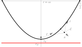
Figure 5: Perturbation along the direction orthogonal to the string in each point with coordinate $l$.

There are different ways to introduce a small time-dependent perturbation. We follow Hashimoto et al. (2018), and perturb the string along the orthogonal direction at each point with coordinate $l$ in the $r-x$ plane, as in Fig. 5. For the unit vector $n^{M}=(0,n^{x},0,0,n^{r})$ orthogonal to $t^{M}$ we have:

$$g_{rr}(r)\left({n}{{}^{r}}\right)^{2}+g_{xx}(r)\left({n}{{}^{x}}\right)^{2} = 1$$ (34)

$$\acute{r}\left(l\right)g_{rr}\left(r\right)\,n^{r}+\acute{x}\left(l\right)g_{xx}\left(r\right)\,n^{x} = 0.$$ (35)

The solution for the components $n^{x}$ and $n^{r}$ is

$${n^{x}}(l)=\sqrt{\frac{g_{rr}}{g_{xx}}}\;\acute{r}(l)\quad\text{,}\quad{n}{{}^{r}}(l)=-\sqrt{\frac{g_{xx}}{g_{rr}}}\;\acute{x}(l)$$ (36)

for an outward perturbation, as in Fig. 5. Introducing a time-dependent perturbation $\xi\left(t,l\right)$ along $n$ one has:

$$r\left(t,l\right) = r_{BG}\left(l\right)+\xi\left(t,l\right)n^{r}\left(l\right),$$

$$x\left(t,l\right) = x_{BG}\left(l\right)+\xi\left(t,l\right)n^{x}\left(l\right),$$ (37)

with $r_{BG}\left(l\right)$ and $x_{BG}\left(l\right)$ the static solutions obtained integrating Eqs. (12) and (13).

To describe the dynamics of the perturbation (assuming it is small), we expand the metric function around the static solution $r_{BG}(l)$ to the third order in $\xi\left(t,l\right)$.

To the third order in $\xi$ the NG action involves a quadratic and a cubic term. The quadratic term has the form:

$$S^{\left(2\right)}=$$

$$\frac{1}{2\pi\alpha^{\prime}}\int\mathrm{d}t\int_{-\infty}^{\infty}\mathrm{d}l\left(C_{tt}\dot{\xi}^{2}+C_{ll}\acute{\xi}^{2}+C_{00}\xi^{2}\right),$$

(38)

with $C_{tt}$, $C_{ll}$ and $C_{00}$ depending on $l$. For the metric in Eq. (3) with a generic metric function $f(r)$ the coefficients $C_{tt}$, $C_{ll}$ and $C_{00}$ read:

$$C_{tt}\left(l\right) =\frac{1}{2r_{BG}\sqrt{f\left(r_{BG}\right)}},$$ (39)

$$C_{ll}\left(l\right) =-\frac{1}{4C_{tt}\left(l\right)},$$

$$C_{00}\left(l\right) =\frac{1}{4r_{BG}^{3}f(r_{BG})^{3/2}}\Bigg{\{}\Big{(}-2r_{BG}^{4}f(r_{BG})^{2}\big{(}2f\left(r_{BG}\right)+r_{BG}f^{\prime}\left(r_{BG}\right)\Big{)}$$

$$+r_{0}^{4}f\left(r_{0}\right)\Big{(}4f\left(r_{BG}\right)^{2}+r_{BG}^{2}f^{\prime}\left(r_{BG}\right)^{2}+r_{BG}f\left(r_{BG}\right)\left(f^{\prime}\left(r_{BG}\right)-r_{BG}f^{\prime\prime}\left(r_{BG}\right)\right)\Big{)}\Bigg{\}}.$$

The coefficients depend on $l$ through $r_{BG}\left(l\right)$. Their expressions for the AdS-RN metric are:

$$C_{tt}\left(l\right) = \frac{r_{BG}^{2}}{2\sqrt{\left(r_{BG}^{2}-r_{H}^{2}\right)\left(r_{BG}^{4}+r_{BG}^{2}r_{H}^{2}-r_{H}^{2}\mu^{2}\right)}},$$

$$C_{ll}\left(l\right) = -\frac{1}{4C_{tt}\left(l\right)},$$

$$C_{00}\left(l\right) = \bigg{(}r_{0}^{6}r_{BG}^{2}\big{(}r_{BG}^{12}-10r_{BG}^{6}r_{H}^{4}\mu^{2}-2r_{H}^{8}\mu^{4}+4r_{BG}^{8}r_{H}^{2}(r_{H}^{2}+\mu^{2})+4r_{BG}^{2}r_{H}^{6}\mu^{2}(r_{H}^{2}+\mu^{2})-r_{BG}^{4}r_{H}^{4}(r_{H}^{2}+\mu^{2})^{2}\big{)}$$ (40)

$$+ r_{BG}^{2}r_{H}^{4}\mu^{2}\big{(}r_{BG}^{12}-10r_{BG}^{6}r_{H}^{4}\mu^{2}-2r_{H}^{8}\mu^{4}+4r_{BG}^{8}r_{H}^{2}(r_{H}^{2}+\mu^{2})+4r_{BG}^{2}r_{H}^{6}\mu^{2}(r_{H}^{2}+\mu^{2})$$

$$- r_{BG}^{4}r_{H}^{4}(r_{H}^{2}+\mu^{2})^{2}\big{)}-r_{0}^{2}\big{(}r_{BG}^{18}-3r_{BG}^{6}r_{H}^{8}\mu^{4}-2r_{H}^{12}\mu^{6}-6r_{BG}^{8}r_{H}^{6}\mu^{2}(r_{H}^{2}+\mu^{2})$$

$$+ 3r_{BG}^{2}r_{H}^{10}\mu^{4}(r_{H}^{2}+\mu^{2})+3r_{BG}^{10}r_{H}^{4}(r_{H}^{2}+\mu^{2})^{2})\big{)}\bigg{)}\frac{1}{r_{0}^{2}\,r_{BG}^{8}\bigg{(}(r_{BG}^{2}-r_{H}^{2})(r_{BG}^{4}+r_{BG}^{2}r_{H}^{2}-r_{H}^{2}\mu^{2})\bigg{)}^{3/2}}.$$

The equation of motion from (38) is

$$C_{tt}\,\ddot{\xi}+\partial_{l}\left(C_{ll}\acute{\xi}\right)-C_{00}\,\xi=0.$$ (41)

For $\xi\left(t,l\right)=\xi\left(l\right)e^{i\omega t}$ this corresponds to

$$\partial_{l}\left(C_{ll}\,\acute{\xi}\right)-C_{00}\,\xi=\omega^{2}C_{tt}\,\xi\,\,,$$ (42)

a Sturm-Liouville equation with weight function $W(l)=-C_{tt}(l)$. We solve Eq. (42) for different values of $r_{0}$ and $\mu$, imposing the boundary conditions $\xi\left(l\right)\xrightarrow{l\rightarrow\pm\infty}0$. The two lowest eigenvalues $\omega_{0}^{2}$ and $\omega_{1}^{2}$, varying $r_{0}$ and $\mu$, are collected in Table 1, and in one case the eigenfunctions $e_{0}\left(l\right)$ and $e_{1}\left(l\right)$ are depicted in Fig. 6.

$r_{0}=1.1$				$r_{0}=1.172$
$\mu$	$\omega_{0}^{2}$	$\omega_{1}^{2}$		$\mu$	$\omega_{0}^{2}$	$\omega_{1}^{2}$
0	-1.370	7.638		0	-0.064	10.458
0.3	-1.235	7.418		0.3	-0.005	10.239
0.6	-0.870	6.748		0.6	0.148	9.574
0.9	-0.388	5.605		0.9	0.324	8.428
1.2	0.006	3.938		1.2	0.397	6.735
$r_{0}=1.18$				$r_{0}=5$
$\mu$	$\omega_{0}^{2}$	$\omega_{1}^{2}$		${\mu}$	$\omega_{0}^{2}$	$\omega_{1}^{2}$
0	0.071	10.754		0	81.726	275.477
0.3	0.124	10.537		0.3	81.706	275.458
0.6	0.258	9.874		0.6	81.648	275.400
0.9	0.406	8.733		0.9	81.551	275.303
1.2	0.449	7.046		1.2	81.415	275.168

Table 1: Eigenvalues $\omega_{0}^{2}$ and $\omega_{1}^{2}$ of Eq. (42) changing the values of $r_{0}$ and $\mu$.

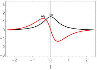
Figure 6: Eigenfunctions $e_{0}\left(l\right)$ (black line) and $e_{1}\left(l\right)$ (red line) of Eq. (42) for $r_{0}=1.172$ and $\mu=0.6$.

There are negative values of $\omega_{0}^{2}$, corresponding to an unstable sector. For $\mu=0$ the system is stabilized as $r_{0}$ increases, with the tip of the string departing from the BH horizon: $\omega_{0}^{2}$ becomes positive for $r_{0}\geq 1.177$. Fixing $r_{0}=1.1$, the lowest lying state is stabilized increasing the chemical potential $\mu$, and $\omega_{0}^{2}$ is positive for $\mu\geq 1.2$. The dependence of $\omega_{0}^{2}$ and $\omega_{1}^{2}$ on $r_{0}$ and $\mu$ is shown in Fig. 7, together with the line demarcating the regions of negative and positive values of $\omega_{0}^{2}$.

The perturbation can be expanded in terms of the first two eigenfunctions $e_{0}$ and $e_{1}$,

$$\xi\left(t,l\right)=c_{0}\left(t\right)e_{0}\left(l\right)+c_{1}\left(t\right)e_{1}\left(l\right),$$ (43)

with the time dependence dictated by the coefficient functions $c_{0}(t)$ and $c_{1}(t)$. Up to a surface term, the cubic action has the expression:

$$S^{\left(3\right)}=\frac{1}{2\pi\alpha^{\prime}}\int\mathrm{d}t\int_{-\infty}^{\infty}\mathrm{d}l\bigg{\{}D_{0}\,\xi^{3}+D_{1}\,\xi\acute{\xi}^{2}+D_{2}\,\xi\dot{\xi}^{2}\bigg{\}}\,\,,$$ (44)

with $D_{0,1,2}$ functions of $l$. This reads, expanding the perturbation $\xi(t,l)$ as in Eq. (43):

$$S^{\left(3\right)} = \frac{1}{2\pi\alpha^{\prime}}\int\mathrm{d}t\int_{-\infty}^{\infty}\mathrm{d}l\Bigg{\{}\Big{(}D_{0}\,e_{0}^{3}+D_{1}\,e_{0}\acute{e}_{0}^{2}\Big{)}c_{0}^{3}\left(t\right)$$ (45)

$$+ \Big{(}3D_{0}\,e_{0}e_{1}^{2}+D_{1}\left(2\acute{e}_{0}e_{1}\acute{e}_{1}+e_{0}\acute{e}_{1}^{2}\right)\Big{)}c_{0}\left(t\right)c_{1}^{2}\left(t\right)+D_{2}\Big{(}e_{0}e_{1}^{2}c_{0}\dot{c}_{1}^{2}+e_{0}^{3}e_{1}^{2}c_{0}\dot{c}_{0}^{2}+2e_{0}e_{1}^{2}\dot{c}_{0}c_{1}\dot{c}_{1}\Big{)}\Bigg{\}}.$$

Upon integration on $l$, an action for $c_{0}(t)$ and $c_{1}(t)$ is obtained summing $S^{(2)}$ and $S^{(3)}$:

$$S^{(2)}+S^{(3)}=\frac{1}{2\pi\alpha^{\prime}}\int\mathrm{d}t\Bigg{[}\sum_{n=0,1}\left(\dot{c}_{n}^{2}-\omega_{n}^{2}c_{n}^{2}\right)+K_{1}c_{0}^{3}+K_{2}c_{0}c_{1}^{2}+K_{3}c_{0}\dot{c}_{0}^{2}+K_{4}c_{0}\dot{c}_{1}^{2}+K_{5}\dot{c}_{0}c_{1}\dot{c}_{1}\Bigg{]}.$$ (46)

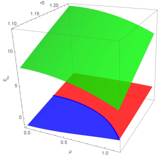
Figure 7: Eigenvalues $\omega_{0}^{2}$ and $\omega_{1}^{2}$ vs $r_{0}$ and $\mu$. The green surface corresponds to $\omega_{1}^{2}$, the red and blue surface to $\omega_{0}^{2}$. The dark blue line demarcates the (blue) region of negative $\omega_{0}^{2}$ from the (red) region of positive $\omega_{0}^{2}$.

The coefficients $K_{1,\dots 5}$ depend on $r_{0}$ and $\mu$, and are collected in Table 2 choosing a set of values for such quantities.

$r_{0}=1.1$	$\mu$	$K_{1}$	$K_{2}$	$K_{3}$	$K_{4}$	$K_{5}$
	0	11.36	21.72	10.58	3.37	6.73
	0.6	7.22	16.76	9.98	3.44	6.88
	1.2	0.81	5.84	8.29	3.64	7.28
$r_{0}=1.172$	$\mu$	$K_{1}$	$K_{2}$	$K_{3}$	$K_{4}$	$K_{5}$
	0	7.63	20.61	8.17	2.69	5.39
	0.6	5.13	17.30	8.04	2.81	5.62
	1.2	0.86	9.30	7.81	3.22	6.44
$r_{0}=1.18$	$\mu$	$K_{1}$	$K_{2}$	$K_{3}$	$K_{4}$	$K_{5}$
	0	7.36	20.64	8.00	2.65	5.29
	0.6	4.97	17.45	7.90	2.76	5.53
	1.2	0.88	9.69	7.76	3.18	6.36
$r_{0}=5$	$\mu$	$K_{1}$	$K_{2}$	$K_{3}$	$K_{4}$	$K_{5}$
	0	-15.01	560.52	7.44	2.84	5.67
	0.6	-14.88	560.57	7.44	2.84	5.67
	1.2	-14.49	560.73	7.46	2.84	5.69

Table 2: $K$ coefficients in Eq. (46) changing the values of $r_{0}$ and $\mu$.

As one can numerically test, in cases corresponding to negative values of $\omega_{0}^{2}$ the action describes the motion of $c_{0}$ and $c_{1}$ in a trap, and in some regions within the potential the kinetic term is negative. As suggested in Hashimoto et al. (2018), it is useful to replace $c_{0,1}\to\tilde{c}_{0,1}$ in the action, with $c_{0}=\tilde{c}_{0}+\alpha_{1}\tilde{c}_{0}^{2}+\alpha_{2}\tilde{c}_{1}^{2}$ and $c_{1}=\tilde{c}_{1}+\alpha_{3}\tilde{c}_{0}\tilde{c}_{1}$, neglecting $\mathcal{O}\left(\tilde{c}_{i}^{4}\right)$ terms, setting the constants $\alpha_{i}$ to ensure the positivity of the kinetic term. We set the constants $\alpha_{1}=-2$, $\alpha_{2}=-0.5$ and $\alpha_{3}=-1$, slightly different from Hashimoto et al. (2018). The replacement stretches the potential stabilizing the time evolution: the dynamics is not affected, and a chaotic behaviour shows up also in the transformed system.

To gain information on chaos we adopt a procedure analogous to the one in Sec. III: we start considering a static solution and perturb it with a small time-dependent fluctuation. However, in this case an analytic computation as in the simplified case in Sec. III cannot be used. Onset of chaos can be investigated constructing Poincaré sections numerically. We show the sections defined by $\tilde{c}_{1}\left(t\right)=0$ and $\dot{\tilde{c}}_{1}\left(t\right)>0$ for bounded orbits within the trap. In the case $r_{H}=1$, $r_{0}=1.1$ and increasing $\mu$ such sections are collected in Fig. 8. For $\tilde{c}_{0}$ near zero the orbits are scattered points depending on the initial conditions. On the other hand, increasing $\mu$ the points in the plot form more regular paths: the effect of switching on the chemical potential is to mitigate the chaotic behavior.

             

Figure 8: Poincaré sections for a time-dependent perturbed string, obtained changing the initial conditions, with $r_{0}=1.1$ and increasing the chemical potential: $\mu=0$ (top row), $\mu=0.03$ (second row), $\mu=0.06$ (third row) and $\mu=0.09$ (bottom row), for $\tilde{c}_{1}=0$ and $\dot{\tilde{c}}_{1}\geq 0$. The plots in the right column enlarge the corresponding ones in the left column in the range of small $\tilde{c}_{0}$, $\dot{\tilde{c}}_{0}$.

For $\mu=1.2$ and $r_{0}=1.1$ the eigenvalue $\omega_{0}^{2}$ becomes positive and the orbits form tori, as one can see in Fig. 9.

Figure 9: Poincaré section in the case $r_{0}=1.1$, $\mu=1.2$, energy $E=1\times 10^{-5}$ with $8\times 10^{3}$ time steps (top panel), $r_{0}=5$, $\mu=0$ and energy $E=1\times 10^{-3}$ (bottom panel).

Moving further away from the horizon, the Poincaré plots for the string dynamics show regular orbits regardless of $\mu$.

The Lyapunov exponents in the four dimensional $c_{0}$, $c_{1}$ phase space can be computed for the different values of $r_{0}$ and $\mu$ using the numerical method in Sandri (1996), briefly described in Appendix A. The results are shown in Figs. 10 and 11.

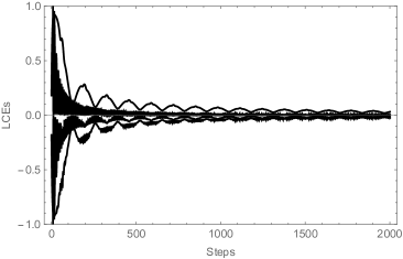
Figure 10: Convergency plots of the four Lyapunov exponents (LCEs) in the case of a string with $r_{0}=1.1$, $\mu=0$ (top panel) and $\mu=0.6$ (bottom panel), and $2\times 10^{3}$ time steps.

Focusing on the system with $r_{0}=1.1$, we have evaluated the convergency plots of the four Lyapunov coefficients, one for each direction of the phase space, varying $\mu$ from $\mu=0$ to $\mu=1.2$. The cases $\mu=0$ and $\mu=0.6$ are displayed in Fig. 10, the other cases are similar. The largest Lyapunov exponent behaves as an exponentially decreasing oscillating function, which can be extrapolated to large number of time steps as shown in Fig. 11.

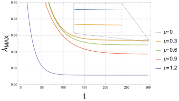
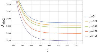
Figure 11: Fit of the largest Lyapunov coefficient $\lambda_{MAX}$ for $r_{0}=1.1$ (top) and $r_{0}=5$ (bottom), varying $\mu$. The local maxima of plots as in Fig. 10 are fitted.

The values resulting from the fit decrease as $\mu$ increases: the effect of the chemical potential is to soften the dependence on the initial conditions, making the string less chaotic.

To investigate the behaviour for different $r_{0}$, we have computed the Lyapunov coefficients for $r_{0}=5$, away from the horizon, and $\mu$ up to $\mu=1.2$. The convergency plots show a rapid convergence of all Lyapunov coefficients towards zero. The result of the fit for large time steps, for different values of $\mu$ is in the same Fig. 11.

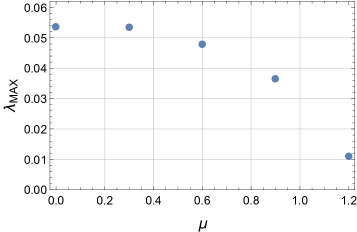
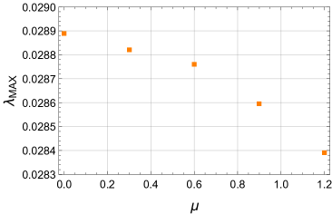
Figure 12: Largest Lyapunov exponent $\lambda_{MAX}$ vs $\mu$, for the tip position $r_{0}=1.1$ (top) and $r_{0}=5$ (bottom).

To summarize, the Poincaré plots show that chaos is produced in the proximity of the BH horizon, and that the dynamics of the string is less chaotic as the chemical potential increases. This is confirmed by the behavior of the largest Lyapunov coefficient, shown in Fig. 12. In all cases the bound Eq. (1) is satisfied: for example, for a system with $r_{0}=1.1$ and $\mu=0.6$ we have $\lambda\simeq(2.7\times 10^{-2})\times 2\pi T_{H}$, close to the value computed for $\mu=0$ in Hashimoto et al. (2018). There are no indications of a relaxed bound as foreseen by Eq. (2).

V Geometry with a dilaton

It is interesting to study a different background, a modification of the AdS-RN with the introduction of a warp factor, used to implement a confining mechanism in holographic models of QCD breaking the conformal invariance Karch et al. (2006). The line element is defined as

$$ds^{2}=e^{-\frac{c^{2}}{r^{2}}}\left(-r^{2}f\left(r\right)dt^{2}+r^{2}d{\bar{x}}^{2}+\frac{1}{r^{2}f(r)}dr^{2}\right),$$

(47)

with the same metric function $f(r)$ in Eq. (4). The Hawking temperature is in Eq. (5) and does not depend on the dilaton parameter $c$. The warp factor mainly affects the IR small $r$ region, and the geometry becomes asymptotically $AdS_{5}$ in the UV $r\to\infty$ region. Introducing a dilaton factor has been used, in a bottom-up approach, to study features of the QCD phenomenology at finite temperature and baryon density, namely the behaviour of the quark and gluon condensates increasing $T$ and $\mu$, the phase diagram, and the in-medium broadening of the spectral functions of two-point correlators Colangelo et al. (2011, 2012a, 2012b, 2013).

The analysis for a time-dependent perturbation of the static string in this background can be carried out following the previously adopted procedure. For the square string in the background (47), the Lyapunov exponent computed at ${\cal O}(L^{2})$ reads:

$$\lambda=2\pi T_{H}\left(1-\frac{L^{2}}{2}\pi T_{H}r_{H}\left(1+\frac{c^{2}}{r_{H}^{2}}\right)\right)\,.$$ (48)

This expression fulfils the bound (1).

To study the dependence of chaos on the dilaton parameter $c$, we inspect the Poincarè plots and compute the Lyapunov exponents. The Poincarè section for $r_{H}=1$, $r_{0}=1.1$, $\mu=0$ and $c=1$ is shown in Fig. 13.

     

Figure 13: Top: Poincaré section for the perturbed string in the background geometry with warp factor (47), for $r_{0}=1.1$, $\mu=0$ and parameter of the dilaton $c=1$, energy $E=1\times 10^{-5}$ and $8\times 10^{3}$ time steps (left plot). The right plot enlarges the left one in the small $\tilde{c}_{0}$, $\dot{\tilde{c}}_{0}$ region. The bottom panels correspond to $c=2$.

For small values of $\tilde{c}_{0}$, $\dot{\tilde{c}}_{0}$ the section shows patterns hinting for a less chaotic system as the constant $c$ increases. This is confirmed by the Poincarè plot for $c=2$, which shows regular orbits also in the phase space region of small $\tilde{c}_{0}$ and $\dot{\tilde{c}}_{0}$. Therefore, increasing the dilaton parameter $c$ the system is less chaotic. It can also be inferred from Fig. 14, where the Lyapunov coefficient for the string with $r_{H}=1$, $r_{0}=1.1$, $\mu=0$ and a few values of $c$ is drawn: the exponent monotonically decreases vs $c$.

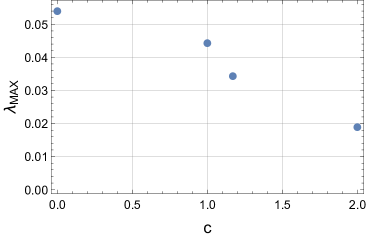
Figure 14: Largest Lyapunov exponent for $r_{0}=1.1$ and $\mu=0$, increasing the dilaton constant $c$.

VI Conclusions

The investigation of a holographic dual of the heavy quark-antiquark system confirms the bounds (1) also in the case of finite baryonic chemical potential. With increasing $\mu$ the system is less chaotic. This agrees with the conclusion obtained considering the charged particle motion in the RN AdS background, for which a reduction of the chaotic behaviour is observed increasing the chemical potential Ageev and Aref’eva (2019). Decrease in chaoticity is also observed for a thermal background involving a dilaton warp factor.

Even though our study is limited to small perturbations of the static string configuration, it seems unlikely that the analysis of large fluctuations would lead to different results: In the case $\mu=0$ the numerical computation of large string fluctuations around the static configuration confirmed the results obtained for small perturbations Hashimoto et al. (2018). This induces us to conclude that the bound (1) continues to hold in the case of finite chemical potential.

A possible extension of our analysis concerns the interplay between chaos and time-dependent background geometry, namely the hydrodynamic metric worked out in Chesler and Yaffe (2009, 2010); Bellantuono et al. (2015, 2017). It would be interesting to establish the existence of a bound analogous to Eq. (1) also in these cases.

Acknowledgements. We thank F. Giannuzzi, A. Mirizzi and S. Nicotri for discussions. This study has been carried out within the INFN project (Iniziativa Specifica) QFT-HEP.

Appendix A Computation of the Lyapunov exponents

To compute the Lyapunov exponents we use a method that can be applied to any n-dimensional dynamical system defined by the equation

$$\dot{x}=F(x)$$ (A.1)

where $\dot{x}=dx/dt$ Sandri (1996). In our case we have a 4-d Hamiltonian dynamical system, with the Hamilton equations obtained from the Legendre transformation of Eq. (46). The point $x(t)$ in the phase space is represented by the variables $\tilde{c}_{0}(t)$, $\tilde{c}_{1}(t)$ and their conjugates momenta. The Lyapunov coefficients, describing the exponential rate growth of the distance between two initially near trajectories, are given by

$$\lambda(x_{0},u_{0}) = \lim_{t\rightarrow\infty}\frac{1}{t}\ln\frac{||u_{t}||}{||u_{0}||}$$ (A.2)

$$= \lim_{t\rightarrow\infty}\frac{1}{t}\ln||D_{x_{0}}f^{t}(x_{0})\cdot u_{0}||.$$

In (A.2) $||u_{0}||$ is the length of the vector representing the initial perturbation between two near trajectories, $u_{t}$ is its evolution at time $t$, and the second equality is obtained from the truncation

$$u_{t}=f^{t}(x_{0}+u_{0})-f^{t}(x_{0})=D_{x_{0}}f^{t}(x_{0})\cdot u_{0},$$ (A.3)

where $f^{t}(x_{0})$ is the solution of Eq. (A.1) with initial condition $x_{0}$. This vector satisfies the so-called variational equation:

$$\dot{\Phi}_{t}(x_{0}) = D_{x}F(f^{t}(x_{0}))\cdot\Phi_{t}(x_{0}),$$

$$\Phi_{0}(x_{0}) = I,$$ (A.4)

where $\Phi_{t}(x_{0})=D_{x_{0}}f^{t}(x_{0})$.

To compute the Lyapunov exponents both Eqs. (A.1) and (A.4) must be solved, namely using a Runge-Kutta method fixing a time step size $s$ and iterated $K$ times in the time interval $T$.

From Eq. (A.2) the largest Lyapunov coefficient (denoted as LCE of order $1$) is obtained. It is useful to generalize the definition for LCEs of order $p$, describing the mean rate growth of a $p$-dimensional volume in the tangent space to the trajectory. They are defined by

$$\lambda^{p}(x_{0},U_{0})=\lim_{t\rightarrow\infty}\frac{1}{t}\ln||\text{Vol}^{p}(D_{x_{0}}f^{t}(U_{0}))||,\,\,\,\,$$ (A.5)

where $U_{0}$ is an initial parallelepiped identified by the initial conditions of the near $p+1$ trajectories. It is always possible to find $p$ linearly independent vectors such that

$$\lambda^{p}(x_{0},U_{0})=\lambda_{1}+\lambda_{2}+\dots+\lambda_{p}.$$ (A.6)

Therefore, each LCE of order $p$ is given by the sum of the $p$ largest LCEs of order 1. For $p=n$ we obtain the mean exponential rate of growth of the phase space volume, given by the sum of the whole spectrum of LCEs. This property can be used to implement an algorithm to evaluate convergency plots of the spectrum of the Lyapunov exponents. The algorithm makes use of the Gram-Schmidt procedure to generate a set of orthonormal vectors. Given an $n$-dimensional solid $U_{0}$ identified by $n$-vectors $\{u_{1},\dots,u_{n}\}$ we have

$$\text{Vol}\{u_{1},\dots,u_{n}\}=||w_{1}||\dots||w_{n}||,$$ (A.7)

where the $w$ vectors are the orthonormal vectors obtained by the Gram-Schmidt procedure on the $u$ vectors. Hence, starting from an initial condition $x_{0}$ in the phase space and an $n\times n$ matrix, that is the initial condition $U_{0}=\{u^{0}_{1},\dots,u^{0}_{n}\}$ for Eq. (A.4), we integrate the system of equations (A.1) and (A.4). After each iteration, the evolution of the tangent vectors is obtained: $U_{1}$ for the first iteration, and so on. The new vectors must be orthogonalized at each iteration. During the $k$-th step the $n$-dimensional volume increase by a factor $||w^{k}_{1}||\dots||w^{k}_{n}||$, where $\{w^{k}_{1},\dots,w^{k}_{n}\}$ is the set of orthogonal vectors calculated from $U_{k}$. From Eq. (A.5) we have for $p=n$:

$$\lambda^{n}(x_{0},U_{0})=\lim_{k\rightarrow\infty}\frac{1}{kT}\sum_{i=1}^{k}\ln(||w^{i}_{1}||\dots||w^{i}_{n}||).\,\,\,\,\,\,\,\,\,\,\,$$ (A.8)

Subtracting $\lambda^{n-1}$ and using the property in Eq. (A.6), we obtain the $n$-th LCE of order $1$:

$$\lambda_{n}=\lim_{k\rightarrow\infty}\frac{1}{kT}\sum_{i=1}^{k}\ln||w^{i}_{n}||.$$ (A.9)

The procedure allows to compute the whole spectrum of the Lyapunov exponents for the total number of steps $K$ reasonably large:

$$\lambda_{1} \sim\frac{1}{KT}\sum_{i=1}^{K}\ln||w^{i}_{1}||,$$ (A.10)

$$\dots,$$

$$\lambda_{n} \sim\frac{1}{KT}\sum_{i=1}^{K}\ln||w^{i}_{n}||.$$

References

- Maldacena et al. (2016) J. Maldacena, S. H. Shenker, and D. Stanford, JHEP 08, 106 (2016), arXiv:1503.01409 [hep-th] .
- Sekino and Susskind (2008) Y. Sekino and L. Susskind, JHEP 10, 065 (2008), arXiv:0808.2096 [hep-th] .
- Susskind (2011) L. Susskind, “Addendum to Fast Scramblers,” (2011), arXiv:1101.6048 [hep-th] .
- Shenker and Stanford (2014) S. H. Shenker and D. Stanford, JHEP 03, 067 (2014), arXiv:1306.0622 [hep-th] .
- Shenker and Stanford (2015) S. H. Shenker and D. Stanford, JHEP 05, 132 (2015), arXiv:1412.6087 [hep-th] .
- Kitaev (2014) A. Kitaev, talk given at the Breakthrough Prize Fundamental Physics Symposium, Kavli Institute for Theoretical Physics, Nov. 10, 2014. Stanford SITP seminars, November 11 and December 18 (2014).
- Polchinski (2015) J. Polchinski, (2015), arXiv:1505.08108 [hep-th] .
- Susskind (2018) L. Susskind, (2018), arXiv:1802.01198 [hep-th] .
- Brown et al. (2018) A. R. Brown, H. Gharibyan, A. Streicher, L. Susskind, L. Thorlacius, and Y. Zhao, Phys. Rev. D 98, 126016 (2018), arXiv:1804.04156 [hep-th] .
- Halder (2019) I. Halder, (2019), arXiv:1908.05281 [hep-th] .
- Maldacena (1998) J. M. Maldacena, Phys. Rev. Lett. 80, 4859 (1998), arXiv:hep-th/9803002 .
- Witten (1998) E. Witten, Adv. Theor. Math. Phys. 2, 253 (1998), arXiv:hep-th/9802150 [hep-th] .
- Gubser et al. (1998) S. Gubser, I. R. Klebanov, and A. M. Polyakov, Phys. Lett. B 428, 105 (1998), arXiv:hep-th/9802109 .
- de Boer et al. (2018) J. de Boer, E. Llabrés, J. F. Pedraza, and D. Vegh, Phys. Rev. Lett. 120, 201604 (2018), arXiv:1709.01052 [hep-th] .
- Dalui et al. (2019) S. Dalui, B. R. Majhi, and P. Mishra, Phys. Lett. B 788, 486 (2019), arXiv:1803.06527 [gr-qc] .
- Avramis et al. (2007) S. D. Avramis, K. Sfetsos, and K. Siampos, Nucl. Phys. B 769, 44 (2007), arXiv:hep-th/0612139 .
- Avramis et al. (2008) S. D. Avramis, K. Sfetsos, and K. Siampos, Nucl. Phys. B 793, 1 (2008), arXiv:0706.2655 [hep-th] .
- Arias and Silva (2010) R. E. Arias and G. A. Silva, JHEP 01, 023 (2010), arXiv:0911.0662 [hep-th] .
- Nunez et al. (2010) C. Nunez, M. Piai, and A. Rago, Phys. Rev. D 81, 086001 (2010), arXiv:0909.0748 [hep-th] .
- Hashimoto et al. (2018) K. Hashimoto, K. Murata, and N. Tanahashi, Phys. Rev. D 98, 086007 (2018), arXiv:1803.06756 [hep-th] .
- Ishii et al. (2017) T. Ishii, K. Murata, and K. Yoshida, Phys. Rev. D 95, 066019 (2017), arXiv:1610.05833 [hep-th] .
- Akutagawa et al. (2019) T. Akutagawa, K. Hashimoto, K. Murata, and T. Ota, Phys. Rev. D 100, 046009 (2019), arXiv:1903.04718 [hep-th] .
- Lee et al. (2009) B.-H. Lee, C. Park, and S.-J. Sin, JHEP 07, 087 (2009), arXiv:0905.2800 [hep-th] .
- Colangelo et al. (2011) P. Colangelo, F. Giannuzzi, and S. Nicotri, Phys. Rev. D 83, 035015 (2011), arXiv:1008.3116 [hep-ph] .
- Sandri (1996) M. Sandri, Mathematica Journal 6, 78 (1996).
- Karch et al. (2006) A. Karch, E. Katz, D. T. Son, and M. A. Stephanov, Phys. Rev. D74, 015005 (2006), arXiv:hep-ph/0602229 [hep-ph] .
- Colangelo et al. (2012a) P. Colangelo, F. Giannuzzi, S. Nicotri, and V. Tangorra, Eur. Phys. J. C 72, 2096 (2012a), arXiv:1112.4402 [hep-ph] .
- Colangelo et al. (2012b) P. Colangelo, F. Giannuzzi, and S. Nicotri, JHEP 05, 076 (2012b), arXiv:1201.1564 [hep-ph] .
- Colangelo et al. (2013) P. Colangelo, F. Giannuzzi, S. Nicotri, and F. Zuo, Phys. Rev. D 88, 115011 (2013), arXiv:1308.0489 [hep-ph] .
- Ageev and Aref’eva (2019) D. S. Ageev and I. Y. Aref’eva, JHEP 01, 100 (2019), arXiv:1806.05574 [hep-th] .
- Chesler and Yaffe (2009) P. M. Chesler and L. G. Yaffe, Phys. Rev. Lett. 102, 211601 (2009), arXiv:0812.2053 [hep-th] .
- Chesler and Yaffe (2010) P. M. Chesler and L. G. Yaffe, Phys. Rev. D 82, 026006 (2010), arXiv:0906.4426 [hep-th] .
- Bellantuono et al. (2015) L. Bellantuono, P. Colangelo, F. De Fazio, and F. Giannuzzi, JHEP 07, 053 (2015), arXiv:1503.01977 [hep-ph] .
- Bellantuono et al. (2017) L. Bellantuono, P. Colangelo, F. De Fazio, F. Giannuzzi, and S. Nicotri, Phys. Rev. D 96, 034031 (2017), arXiv:1706.04809 [hep-ph] .