Towards a QMC-based density functional including finite-range effects:
excitation modes of a ³⁹K quantum droplet

Abstract

Some discrepancies between experimental results on quantum droplets made of a mixture of ³⁹K atoms in different hyperfine states and their analysis within extended Gross-Pitaevskii theory (which incorporates beyond mean-field corrections) have been recently solved by introducing finite-range effects into the theory. Here, we study the influence of these effects on the monopole and quadrupole excitation spectrum of extremely dilute quantum droplets using a density functional built from first-principles quantum Monte Carlo calculations, which can be easily introduced in the existing Gross-Pitaevskii numerical solvers. Our results show differences of up to $20\%$ with those obtained within the extended Gross-Pitaevskii theory, likely providing another way to observe finite-range effects in mixed quantum droplets by measuring their lowest excitation frequencies.

I Introduction

Ultracold gases serve as a unique platform for understanding quantum many-body physics Bloch et al. (2008). This notoriously hard problem is often reduced to the effective single-particle picture when the interactions are very weak and the density is very low Pethick and Smith (2008); Pitaevskii and Stringari (2016). Because of its simplicity and predictive power, the mean field approach has become a standard (or a first starting point) to study the properties of ultracold gases.

The accuracy of mean-field theories to address dilute quantum gases is expectable, as nearly all experiments are performed at very low values of the gas parameter $\rho a^{3}$, $\rho$ being the atom number density and $a$ the s-wave scattering length describing the interparticle interactions. This allows for a perturbative approach à la Bogoliubov Bogoliubov (1947), where static and dynamic properties are well described by the Gross-Pitaevskii equation. However, as the density and/or the interaction strength increases, the system becomes more correlated and out of the range of applicability of perturbation theories. It is a priori difficult to know when the perturbative approach is no longer valid. Thus, it is essential to supplement the theory with developments Cikojević et al. (2018, 2019); Parisi and Giorgini (2020); Parisi et al. (2019); Staudinger et al. (2018); Petrov and Astrakharchik (2016); Bombin et al. (2017); Ancilotto et al. (2018a); Hu and Liu (2020a, b); Ota and Astrakharchik (2020) aiming at verifying the range of applicability of the mean-field approach and disclosing the role played by higher-order effects.

A promising system for investigating quantum many-body effects, going beyond mean-field theory, is the self-bound Bose-Bose mixture first proposed by Petrov Petrov (2015). In this mixture, with repulsive intraspecies and attractive interspecies short-range interactions, the unstable attractive mean-field energy is balanced out by a repulsive beyond mean-field term (the Lee-Huang-Yang (LHY) term) Lee et al. (1957), resulting in a liquid droplet resembling the well-known ⁴He droplets Barranco et al. (2006), but with a far smaller density. So far, a Bose-Bose droplet state has been observed in a mixture of two ³⁹K hyperfine states Cabrera et al. (2018); Semeghini et al. (2018); Cheiney et al. (2018), and in an heterogeneous mixture of ⁴¹K-⁸⁷Rb atoms D’Errico et al. (2019).

In the first experimental observation Cabrera et al. (2018), discernible differences were observed between the experiment and the results of the mean-field (MF) theory extended with an LHY term. Quite recently, it has been reported Cikojević et al. (2020) that the agreement between theory and experiment improves notably when finite-range effects are properly taken into account. For the particular mixture of two hyperfine states of ³⁹K atoms, we know two scattering parameters in each of the interaction channels Tanzi et al. (2018), the s-wave scattering length $a$ and the effective range $r^{\rm eff}$, which are the first two coefficients in the expansion of the s-wave phase shift in the scattering between two atoms Newton (2013)

$$k\cot\delta(k)=-\dfrac{1}{a}+\dfrac{1}{2}r^{\rm eff}k^{2}+\mathcal{O}(k^{4}).$$ (1)

The non-zero (in fact quite large) effective ranges open a promising new regime in quantum mixtures which go beyond the usual mean-field theory corrected with the LHY term (MF+LHY) Tononi (2019); Tononi et al. (2018); Salasnich (2017). A large effective range means that the interaction between atoms is far from the contact Dirac $\delta$-interaction usually employed for dilute Bose gases.

In a previous work Cikojević et al. (2020), some of us have performed diffusion Monte Carlo (DMC) calculations Boronat and Casulleras (1994); Giorgini et al. (1999) using model potentials that reproduce both scattering parameters, obtaining the equation of state for a ³⁹K mixture in the homogeneous liquid phase. We concluded that one could reproduce the critical atom number determined in the experiment Cabrera et al. (2018) only for the model potentials which incorporate the correct effective range. This critical number is a static property of the quantum droplet at equilibrium. Besides a good knowledge of the equilibrium properties of a quantum many-body system, determining the excitation spectrum is essential to unveil its microscopic structure.

In the present work, we present a study of the monopole and quadrupole excitation spectrum of a ³⁹K quantum droplet using the QMC functional introduced in Ref. Cikojević et al. (2020), which correctly describes the inner part of large drops, constituting an extension to the MF+LHY theory. The excitation spectrum of these droplets has already been calculated within the MF+LHY approach Petrov (2015); Jørgensen et al. (2018). Our goal is to make visible the appearance of any beyond-LHY effect arising from the inclusion of the effective range in the interaction potentials.

This paper is organized as follows. We build in Sec. II the QMC density functional, in the local density approximation (LDA), and compare it with the MF+LHY approach, which can be expressed in a similar form. In Sec. III, we give details on the application of the density functional method, static and dynamic, to the obtainment of the ground state and excitation spectrum of quantum droplets. In Sec. IV, we report the results of the monopole and quadrupole frequencies obtained with the QMC functional and compare them with the MF+LHY predictions. Finally, a summary and outlook are presented in Sec. V.

II The QMC Density Functional

We shall consider ³⁹K mixtures at the optimal relative atom concentration yielded by the mean-field theory, namely $N_{1}/N_{2}=\sqrt{a_{22}/a_{11}}$ Petrov (2015). For these mixtures, we have shown that the energy per atom in the QMC approach can be accurately written as Cikojević et al. (2020)

$$\dfrac{E}{N}=\alpha\rho+\beta\rho^{\gamma}\ ,$$ (2)

where $\rho$ is the total atom number density. The parameters $\alpha$, $\beta$, and $\gamma$ have been determined by fits to the DMC results for the model potentials satisfying the s-wave scattering length and effective range, given in Table 1. Parameters appearing in Eq. (2) are collected in Table 2, for three values of the magnetic field ($B$). The QMC approach does not yield a universal expression for $E/N$, as it depends on the value of the applied $B$. For the optimal concentration, the MF+LHY energy per particle can be cast in a similar expression

$$\dfrac{E/N}{|E_{0}|/N}=-3\left(\dfrac{\rho}{\rho_{0}}\right)+2\left(\dfrac{\rho}{\rho_{0}}\right)^{3/2}\ ,$$ (3)

where $E_{0}/N$ and $\rho_{0}$ are the energy per atom and atom density at equilibrium,

$$E_{0}/N=\dfrac{25\pi^{2}\hbar^{2}|a_{12}+\sqrt{a_{11}a_{22}}|^{3}}{768ma_{22}a_{11}\left(\sqrt{a_{11}}+\sqrt{a_{22}}\right)^{6}}$$ (4)

and

$$\rho_{0}=\dfrac{25\pi}{1024a_{11}^{3}}\dfrac{\left(a_{12}/a_{11}+\sqrt{a_{22}/a_{11}}\right)^{2}}{\left(a_{22}/a_{11}\right)^{3/2}\left(1+\sqrt{a_{22}/a_{11}}\right)^{4}}\ .$$ (5)

In Eqs. (4) and (5), $m$ is the mass of a ³⁹K atom and $a_{ij}$ are the three different s-wave scattering lengths. MF+LHY theory is thus universal if it is expressed in terms of $\rho_{0}$ and $E_{0}$. According to this theory, the droplet properties do not change separately on $N$ and $a_{ij}$ but rather combined through

$$\dfrac{N}{\tilde{N}}=\dfrac{3\sqrt{6}}{5\pi^{2}}\dfrac{\left(1+\sqrt{a_{22}/a_{11}}\right)^{5}}{\left|a_{12}/a_{11}+\sqrt{a_{22}/a_{11}}\right|^{5/2}}\ ,$$ (6)

where $\tilde{N}$ is a dimensionless parameter Petrov (2015). Additionally, the healing length corresponding to the mixture is

$$\dfrac{\xi}{a_{11}}=\dfrac{8\sqrt{6}}{5\pi}\sqrt{\dfrac{a_{22}}{a_{11}}}\dfrac{(1+\sqrt{a_{22}/a_{11}})^{3}}{\left|a_{12}/a_{11}+\sqrt{a_{22}/a_{11}}\right|^{3/2}}\ .$$ (7)

Table 1: Scattering parameters, i.e. s-wave scattering length $a$ and effective range $r^{\rm eff}$ (in units of Bohr radius $a_{0}$) as a function of $B$ Roy et al. (2013).

$B({\rm G})$	$a_{11}(a_{0})$	$r_{11}^{\rm eff}(a_{0})$	$a_{22}(a_{0})$	$r_{22}^{\rm eff}(a_{0})$	$a_{12}(a_{0})$	$r_{12}^{\rm eff}(a_{0})$
56.230	63.648	-1158.872	34.587	578.412	-53.435	1021.186
56.453	70.119	-1150.858	34.136	599.143	-53.333	1023.351
56.639	76.448	-1142.642	33.767	616.806	-53.247	1025.593

Table 2: Parameters of the QMC energy per atom calculated at several magnetic fields $B$, assuming $\rho_{1}/\rho_{2}=\sqrt{a_{22}/a_{11}}$, satisfying the s-wave scattering length $a$ and effective range $r^{\rm eff}$ given in Table 1. $\alpha$ is in $\hbar^{2}a_{11}^{2}/(2m)$ units, $\beta$ is in $\hbar^{2}a_{11}^{3\gamma-2}/(2m)$ units, $m$ being the mass of a ³⁹K atom, and $\gamma$ is dimensionless.

$B({\rm G})$	$\alpha$	$\beta$	$\gamma$
56.230	-0.812	5.974	1.276
56.453	-0.423	8.550	1.373
56.639	-0.203	12.152	1.440

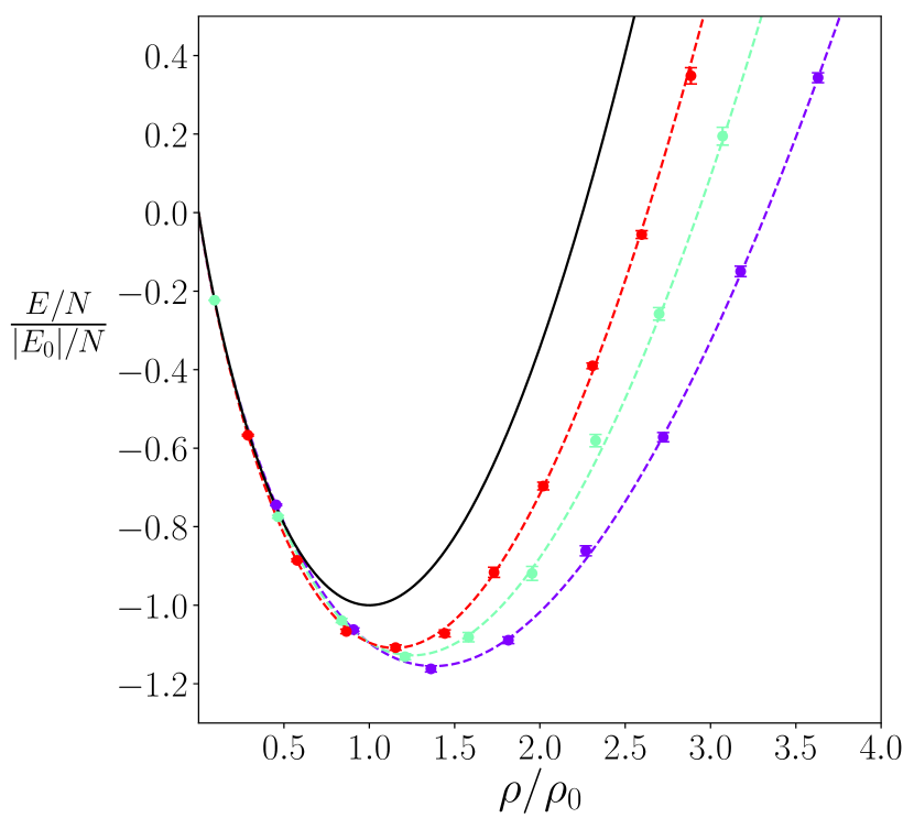
Figure 1: DMC energy per particle as a function of the density. From bottom (blue dots) to top (red dots), the results correspond to magnetic fields $B$=56.23, 56.453 and 56.639 G. Calculations were performed for the mean-field optimal ratio $\rho_{2}/\rho_{1}=\sqrt{{a_{11}/a_{22}}}$. The energy per atom and atom density are normalized to the $|E_{0}|/N$ and $\rho_{0}$ MF+LHY values obtained from Eqs. (4) and (5), respectively. The dashed lines are fits in the form $E/N=\alpha\rho+\beta\rho^{\gamma}$. The black solid line corresponds to the MF+LHY theory, Eq. (3).

The energy per atom Eq. (2) allows one to readily introduce, within LDA, a density functional whose interacting part is

$$\mathcal{E}_{\rm int}=\rho\frac{E}{N}=\alpha\rho^{2}+\beta\rho^{\gamma+1}\ .$$ (8)

A similar expression holds in the MF+LHY approach. In the homogeneous phase, one may easily obtain the pressure

$$p(\rho)=\rho^{2}\dfrac{\partial}{\partial\rho}\left(\dfrac{E}{N}\right)=\alpha\rho^{2}+\beta\gamma\rho^{\gamma+1}$$ (9)

and incompressibility

$$\kappa(\rho)=\rho\frac{\partial p}{\partial\rho},$$ (10)

which can be written as

$$\kappa(\rho)=\rho^{2}\frac{\partial^{2}\mathcal{E}_{\rm int}}{\partial\rho^{2}}=\rho^{2}\left\{2\frac{\partial}{\partial\rho}\left(\frac{E}{N}\right)+\rho\frac{\partial^{2}}{\partial\rho^{2}}\left(\frac{E}{N}\right)\right\}.$$ (11)

Figure 1 shows the DMC energy per atom as a function of the density for selected values of the magnetic field, together with the result for the MF+LHY theory. It is worth noticing the rather different equations of state yielded by the QMC functional and MF+LHY approaches. The QMC approach yields a substantially larger equilibrium density and more binding. The QMC incompressibility is also larger, as can be seen in Fig. 2; at first sight, this seems to be in contradiction with the results in Fig. 1, which clearly indicate that the curvature of the $E/N$ vs $\rho$ curve at equilibrium ($\partial(E/N)/\partial\rho=0$ point) is smaller for the QMC functionals than for the MF+LHY approach. However, this is compensated by the larger QMC value of the atom density at equilibrium, see Eq. (11) and Fig. 3, where we show the ratio of QMC and MF+LHY equilibrium densities. Besides its importance for a quantitative description of the monopole droplet oscillations addressed here, inaccurate incompressibility may affect the description of processes where the liquid-like properties of quantum droplets play a substantial role, as e.g. droplet-droplet collisions Ferioli et al. (2019).

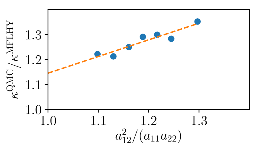
Figure 2: DMC over MF+LHY incompressibility ratio at equilibrium for the magnetic fields considered in Ref. Cikojević et al. (2020). The dashed line is a linear fit to the points.

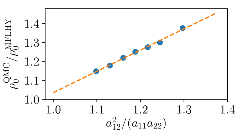
Figure 3: DMC over MF+LHY equilibrium density ratio for the magnetic fields considered in Ref. Cikojević et al. (2020). The dashed line is a linear fit to the points.

Table 3: Surface tension of a ³⁹K Bose-Bose mixture at the MF+LHY optimal mixture composition in $10^{-8}\times\hbar^{2}/(ma_{11}^{4})$ units.

$B({\rm G})$	$\sigma_{\rm MF+LHY}$	$\sigma_{\rm QMC}$
56.230	35.1	48.8
56.453	9.31	12.2
56.639	1.21	1.46

Another fundamental property of the liquid is the surface tension $\sigma$ of the free-surface. Remarkably, for simple functionals as the QMC and MF+LHY ones discussed in this work, its value can be obtained by simple quadrature Stringari and Treiner (1987)

$$\sigma=2\int_{0}^{\rho_{0}}d\rho\left[\left(\dfrac{\hbar^{2}}{8m}\right)\left(\alpha\rho+\beta\rho^{\gamma}-\mu\right)\right]^{1/2},$$ (12)

where $\mu$ is the chemical potential evaluated at the equilibrium density. The surface tension of several QMC functionals, i.e. functionals corresponding to different magnetic fields, is given in Table 3. As can be seen, QMC functionals yield consistently higher values of the surface tension than the MF+LHY approach. Within MF+LHY, the surface tension can be written in terms of the equilibrium density (5) and healing length (7), $\sigma_{\rm MF+LHY}=3(1+\sqrt{3})\rho_{0}\hbar^{2}/(35m\xi)$ Petrov (2015).

III The LDA-DFT approach

III.1 Statics

Once $\mathcal{E}_{\rm int}[\rho]$ has been obtained, we have used density functional theory (DFT) to address the static and dynamic properties of ³⁹K droplets similarly as for superfluid ⁴He droplets Ancilotto et al. (2017). Within DFT, the energy of the quantum droplet at the optimal composition mixture is written as a functional of the atom density $\rho({\mathbf{r}})$ as

$$E[\rho]=T[\rho]+E_{c}[\rho]=\frac{\hbar^{2}}{2m}\int d{\mathbf{r}}|\nabla\Psi({\mathbf{r}})|^{2}+\int d{\mathbf{r}}\,{\cal E}_{\rm int}[\rho],$$ (13)

where the first term is the kinetic energy, and the effective wavefunction $\Psi({\mathbf{r}})$ of the droplet is related to the atom density as $\rho({\mathbf{r}})=|\Psi({\mathbf{r}})|^{2}$. The equilibrium configuration is obtained by solving the Euler-Lagrange equation arising from the functional minimization of Eq. (13)

$$\left\{-\frac{\hbar^{2}}{2m}\nabla^{2}+\frac{\partial{\cal E}_{int}}{\partial\rho}\right\}\Psi\equiv{\cal H}[\rho]\,\Psi=\mu\Psi,$$ (14)

where $\mu$ is the chemical potential corresponding to the number of ³⁹K atoms in the droplet, $N=\int d{\bf r}|\Psi({\bf r})|^{2}$.

The time-dependent version of Eq. (14) is obtained minimizing the action and adopts the form

$$i\hbar\frac{\partial}{\partial t}\Psi({\mathbf{r}},t)={\cal H}[\rho]\,\Psi({\mathbf{r}},t).$$ (15)

We have implemented a three-dimensional numerical solver based on the Trotter decomposition of the time-evolution operator with second-order accuracy in the time-step $\Delta t$  Chin et al. (2009)

$$e^{-i{\cal H}\Delta t}=e^{-i\Delta tV({\bm{R}}^{\prime})/2}e^{-i\Delta tK}e^{-i\Delta tV({\bm{R}})/2}+\mathcal{O}(\Delta t^{3})\ ,$$ (16)

with $K$ and $V$ being the kinetic and interaction terms in Eq. (14). Within this scheme, it is possible to obtain both the ground state and the dynamical evolution. Indeed, reformulating the problem via a Wick rotation $t=-i\tau$, the propagation of a wavefunction in imaginary time $\tau$ leads to the ground-state equilibrium solution.

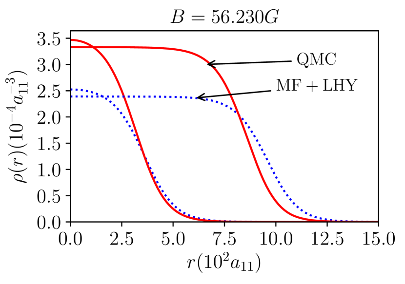
Figure 4: Density profiles of two ³⁹K quantum droplets corresponding to a small $(\tilde{N}-\tilde{N}_{c})^{1/4}=3$, and to a large droplet $(\tilde{N}-\tilde{N}_{c})^{1/4}=6$, where $\tilde{N}_{c}=18.65$ is the critical number below which the droplet becomes unstable within the MF+LHY theory Petrov (2015). Solid lines, QMC functional; dotted lines, MF+LHY approach.

Figure 4 shows the density profile of two droplets, one corresponding to a small gaussian-like droplet and the other to a large saturated one. They have been obtained within the QMC ($B=56.230$ G) functional and MF+LHY methods. The sizeable difference between the profiles yielded by both approaches reflects the different value of their equilibrium densities, see Fig. 3.

III.2 Real-time dynamics and excitation spectrum

The multipole excitation spectrum of a quantum droplet can be obtained e.g. by solving the equations obtained linearizing Eq. (15) Dalfovo et al. (1999); Petrov (2015); Baillie et al. (2017). We have used an equivalent method based on the Fourier analysis of the real-time oscillatory response of the droplet to an appropriated external field Stringari and Vautherin (1979); Pi et al. (1986). The method, which we outline now, bears clear similarities with the experimental procedure to access to some excited states of confined Bose-Einstein condensates (BEC) Jin et al. (1996); Altmeyer et al. (2007).

A droplet at the equilibrium, whose ground-state effective wavefunction $\Psi({\mathbf{r}})$ is obtained by solving the DFT Eq. (14), is displaced from it by the action of a static external one-body field $Q$ whose intensity is controlled by a parameter $\lambda$. The new equilibrium wavefunction $\Psi^{\prime}({\mathbf{r}})$ is determined by solving Eq. (14) for the constrained Hamiltonian ${\cal H}^{\prime}$

$${\cal H}\rightarrow{\cal H}^{\prime}={\cal H}+\lambda Q.$$ (17)

If $\lambda$ is small enough so that $\lambda Q$ is a perturbation and linear response theory applies, switching off $Q$ and letting $\Psi^{\prime}({\mathbf{r}})$ evolve in time according to Eq. (15), $\langle Q(t)\rangle$ will oscillate around the equilibrium value $Q_{eq}=\langle\Psi({\mathbf{r}})|Q|\Psi({\mathbf{r}})\rangle$. Fourier analyzing $\langle Q(t)\rangle$, one gets the non-normalized strength function corresponding to the excitation operator $Q$, which displays peaks at the frequency values corresponding to the excitation modes of the droplet. Specific values of $\lambda$ that we use are in the range from $\lambda=10^{-13}$ to $10^{-15}$ for the monopole modes, and $\lambda=10^{-15}$ to $10^{-17}$ for the quadropole modes, with $\lambda$ being measured in $\hbar^{2}/(2ma_{11}^{4})$ units, and the smaller values corresponding to larger magnetic fields, i.e. less correlated drops.

IV Results

We have used as excitation fields the monopole $Q_{0}$ and quadrupole $Q_{2}$ operators

$$Q_{\rm 0} = \sum_{i}^{N}r_{i}^{2}$$ (18)

$$Q_{\rm 2} = \sum_{i}^{N}\left(r_{i}^{2}-3z_{i}^{2}\right)$$ (19)

which allows one to obtain the $\ell=0$ and 2 multipole strengths. The $\ell=0$ case corresponds to pure radial oscillations of the droplet and for this reason it is called “breathing” mode. In a pure hydrodynamical approach, its frequency is determined by the incompressibility of the liquid and the radius of the droplet Bohigas et al. (1979); Pitaevskii and Stringari (2016).

We have propagated the excited state $\Psi^{\prime}({\mathbf{r}})$ for a very long period of time, storing $\langle Q(t)\rangle$ and Fourier analyzing it. Fig. 5 (left) shows $\langle Q_{0}(t)\rangle$ for ³⁹K quantum droplets of different sizes. We choose the same scale of particle numbers (x-axis) as in Ref. Petrov (2015), as the monopole frequency $\omega_{0}$ close to the instability point $\tilde{N}_{c}=18.65$ is directly proportional to $(\tilde{N}-\tilde{N}_{c})^{1/4}$ Petrov (2015). Whereas a harmonic behavior is clearly visible for the largest droplets, as corresponding to a single-mode excitation, for small droplets the radial oscillations are damped and display different oscillatory behaviors (beats), anticipating the presence of several modes in the monopole strength, as the Fourier analysis of the signal unveils.

Figure 5 (right) displays the monopole strength function in logarithmic scale as a function of the excitation frequency. The solid vertical line represents the frequency $|\mu|/\hbar$ corresponding to the atom emission threshold, i.e. the absolute value of the atom chemical potential, $|\mu|$. It can be seen that for $(\tilde{N}-18.65)^{1/4}=5.1$ the strength is in the continuum frequency region above $|\mu|/\hbar$. Hence, self-bound small ³⁹K droplets, monopolarly excited, have excited states (resonances) that may decay by atom emission Petrov (2015); Ferioli et al. (2020). This decay does not imply that the droplet breaks apart; it just loses the energy deposited into it by emitting a number of atoms, in a way similar to the decay of some states appearing in the atomic nucleus, the so-called “giant resonances” Bohigas et al. (1979). We want to stress that the multipole strength is not normalized, as it depends on the value of the arbitrary small parameter $\lambda$. However, the relative intensity of the peaks for a given droplet is properly accounted for in this approach.

A similar analysis for the quadrupole mode is presented in Fig. 6. In this case, we have found a more harmonic behavior for $\langle Q_{2}(t)\rangle$, and therefore the quadrupole strength function is dominated by one single peak.

Figures 5 and 6 show an interesting evolution of the strength function from the continuum to the discrete part of the frequency spectrum as the number of atoms in the droplet increases. For small $N$ values, but still corresponding to self-bound quantum droplets, the spectrum is dominated by a broad resonance that may decay by atom emission. The $\langle Q(t)\rangle$ oscillations are damped, and when several resonances are present (monopole case), distinct beats appear in the oscillations.

This remarkable evolution of the monopole and quadrupole spectrum has also been found for ³He and ⁴He droplets Serra et al. (1991); Barranco and Hernández (1994). In the ⁴He case, it has been experimentally confirmed by detecting “magic” atom numbers in the size distribution of ⁴He droplets which correspond to especially stable droplets Brühl et al. (2004). The magic numbers occur at the threshold sizes for which the excitation modes of the droplet, as calculated by the diffusion Monte Carlo method, are stabilized when they pass below the atom emission energy. This constituted the first experimental confirmation for the energy levels of ⁴He droplets. On the other hand, in confined BECs, the energy of the breathing mode is obtained by direct analysis of the radial oscillations of the atom cloud Pitaevskii and Stringari (2016).

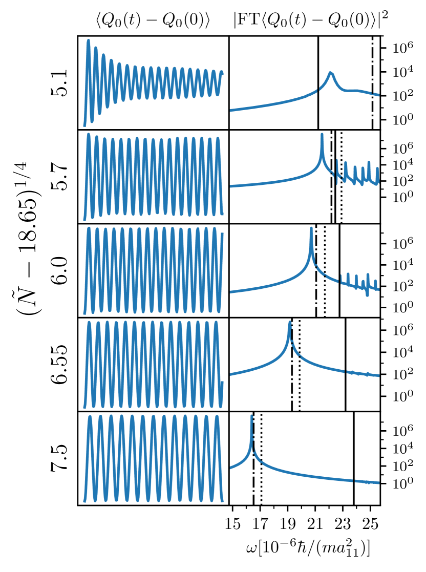
Figure 5: Time evolution of the monopole moment $\langle Q_{0}(t)\rangle$ and strength function (right) for ³⁹K quantum droplets of different sizes obtained using the QMC functional at $B=56.230$ G. In the right panels, the vertical solid line corresponds to the frequency $|\mu|/\hbar$ corresponding to the atom emission energy $|\mu|$, and the dotted and dash-dotted lines to the $E_{3}/\hbar$ and $E_{1}/\hbar$ frequencies, obtained by the sum rules in Eq. (23) and (20), respectively.

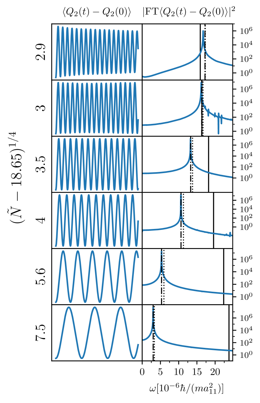
Figure 6: Time evolution of the quadrupole moment $\langle Q_{2}(t)\rangle$ and strength function (right) for ³⁹K quantum droplets of different sizes obtained using the QMC functional at $B=56.230$ G. In the right panels, the vertical solid line corresponds to the frequency $|\mu|/\hbar$ corresponding to the atom emission energy $|\mu|$, and the dotted and dash-dotted lines to the $E_{3}/\hbar$ and $E_{1}/\hbar$ frequencies, obtained by the sum rules in Eq. (24) and (21), respectively.

We show in Fig. 7 the breathing and quadrupole frequencies, corresponding to the more intense peaks, as a function of the number of atoms obtained with the QMC functional and the MF+LHY approach. For the latter, our results are in full agreement with those reported by Petrov using the Bovoliubov-de Gennes method Petrov (2015), which is fully equivalent to ours. The results are plotted in the universal units of the MF+LHY theory. We find that the QMC functional predicts systematically larger monopole and quadrupole frequencies in all the range of particle numbers we have studied. Additionally, as we change the magnetic field, i.e. the scattering parameters, QMC predictions do not fall on the same curve, meaning that the QMC functional breaks the MF+LHY universality.

When the multipole strength is concentrated in a single narrow peak, it is possible to estimate the peak frequency using the sum rules approach Bohigas et al. (1979); Pitaevskii and Stringari (2016). Sum rules are energy moments of the strength function that, for some excitation operators, can be written as compact expressions involving expectation values on the ground state configuration. For the multipole operators considered here, two such sum rules are the linear-energy $m_{1}$ and cubic-energy $m_{3}$ sum rules. The inverse-energy sum rule $m_{-1}$ can be obtained from a constrained calculation involving the Hamiltonian ${\cal H}^{\prime}$ of Eq. (17). Once determined, these three sum rules may be used to define two average energies $E_{1}=\sqrt{m_{1}/m_{-1}}$ and $E_{3}=\sqrt{m_{3}/m_{1}}$ expecting, bona fide, that they are good estimates of the peak energy.

For the monopole and quadrupole modes, the $E_{1}$ energies are Bohigas et al. (1979)

$$E_{1}(\ell=0)=\sqrt{-\dfrac{4\hbar^{2}}{m}\,\dfrac{\left<r^{2}\right>}{\left(\partial\left<Q_{0}\right>/\partial\lambda\right)\rvert_{\lambda=0}}}$$ (20)

and

$$E_{1}(\ell=2)=\sqrt{-\dfrac{8\hbar^{2}}{m}\,\dfrac{\left<r^{2}\right>}{\left(\partial\left<Q_{2}\right>/\partial\lambda\right)\rvert_{\lambda=0}}}\;,$$ (21)

with $\lambda$ being the parameter in the constrained Hamiltonian ${\cal H}^{\prime}$, Eq.(17), and $\left<r^{2}\right>=\displaystyle\int d{\bm{r}}\rho(r)r^{2}/N$ evaluated at $\lambda=0$. The frequencies corresponding to these energies are drawn in Figs. 5 and 6 as vertical dash-dotted lines. Except for small droplets, for which the monopole strength is very fragmented, one can see that they are good estimates of the peak frequency.

Closed expressions for the $E_{3}$ averages can be easiliy obtained for the monopole and the quadrupole modes Bohigas et al. (1979); Pitaevskii and Stringari (2016). For the sake of completeness, we present the result obtained for the QMC functional.

Defining

$$E_{\alpha} = \alpha\int d\mathbf{r}\rho^{2}(\mathbf{r})$$

$$E_{\beta} = \beta\int d\mathbf{r}\rho^{\gamma+1}(\mathbf{r})$$

$$\langle T\rangle = \frac{\hbar^{2}}{2m}\int d{\mathbf{r}}|\nabla\Psi({\mathbf{r}})|^{2}\;,$$ (22)

where $\Psi({\mathbf{r}})$ and $\rho(\mathbf{r})$ are those of the equilibrium configuration, we have

$$E_{3}(\ell=0)=\left[\frac{\hbar^{2}}{Nm\langle r^{2}\rangle}\right]^{1/2}[4\langle T\rangle+9(E_{\alpha}+\gamma^{2}E_{\beta})]^{1/2}$$ (23)

$$E_{3}(\ell=2)=\left[\frac{\hbar^{2}}{Nm\langle r^{2}\rangle}\right]^{1/2}[4\langle T\rangle]^{1/2}\;.$$ (24)

We have $E_{3}(\ell=2)<E_{3}(\ell=0)$. The $\omega_{3}=E_{3}/\hbar$ frequencies are shown in Figs. 5 and 6 as vertical dotted lines. It can be seen that even when the strength is concentrated in a single peak, $\omega_{3}$ is a worse estimate of the peak frequency than $\omega_{1}=E_{1}/\hbar$. This is likely so because $m_{3}$ gets contributions from the high energy part of the spectrum. At variance, since contributions to $m_{-1}$ mainly come from the low energy part of the spectrum, $\omega_{1}$ is better suited for estimating the peak frequency.

The relative differences between the MF+LHY theory and the QMC functional for monopole and quadrupole frequencies are presented in Fig. 8. As the magnetic field increases, the droplet is more correlated and differences of even $20\%$ can be observed.

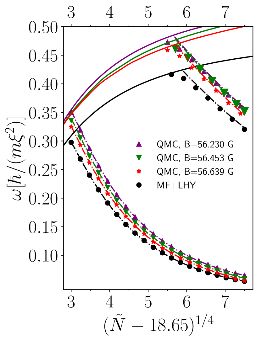
Figure 7: Breathing (upper points) and quadrupole (lower points) frequencies as a function of the total atom number in units of $\tilde{N}$. Points are the results obtained from QMC and MF+LHY TDDFT calculations, and dashed lines are the $E_{1}/\hbar$ frequencies from the sum-rule approach (Eqs. (20) and (21)). Full lines represent the frequency corresponding to the absolute value of the droplet chemical potential $|\mu|$, corresponding to the legend from top to bottom

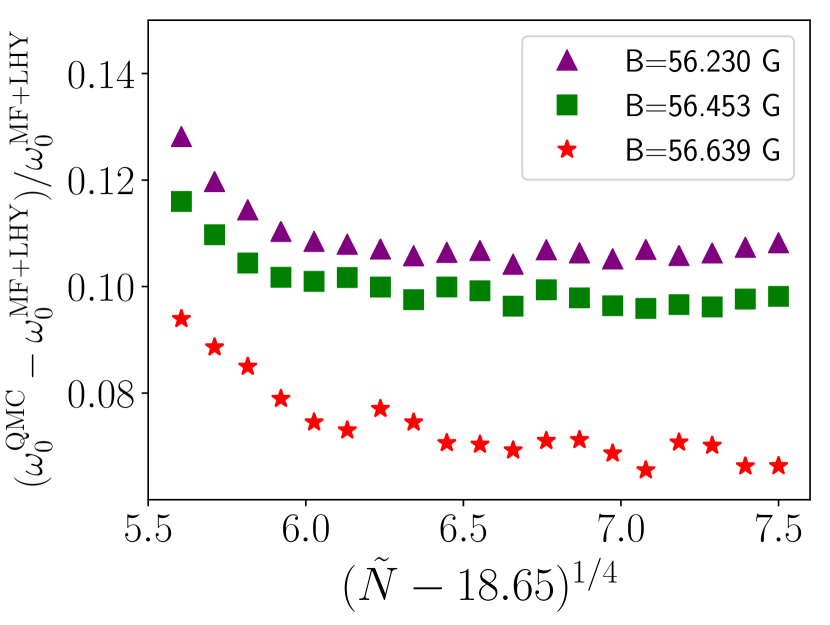
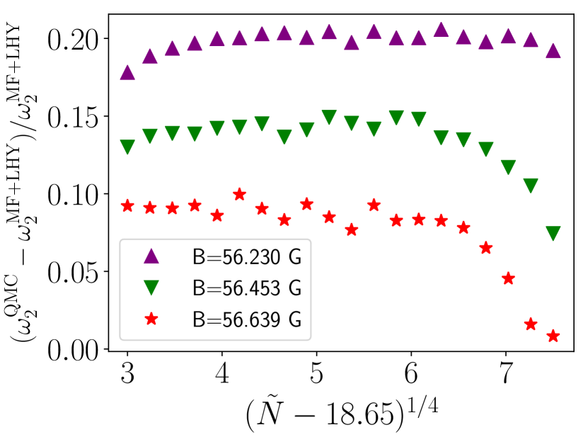
Figure 8: Relative frequency difference between QMC and MF+LHY TDDFT calculations for quadrupole (bottom figure) and monopole modes (top figure) as a function of the total atom number in units of $\tilde{N}$.

We finally compare in more detail the frequencies obtained with the QMC and MF+LHY functionals at $B=56.230$ G for $\tilde{N}=100$ and $\tilde{N}=1010$, which correspond to $N=7\times 10^{4}$ and $N=7.1\times 10^{5}$, respectively. Although it might require rather large droplets to observe neat breathing oscillations, systems with $\tilde{N}>100$, for which clean quadrupole modes show up (see Fig. 7), are already accessible in experiments Cabrera et al. (2018); Semeghini et al. (2018); Ferioli et al. (2019); D’Errico et al. (2019). For $N=7\times 10^{4}$, the quadrupole frequencies are $\omega_{2}^{\rm QMC}=2323\,{\rm Hz}$ and $\omega_{2}^{\rm MF+LHY}=1972\,{\rm Hz}$, i.e. oscillation periods $\tau_{2}^{\rm QMC}=2.70\,{\rm ms}$ and $\tau_{2}^{\rm MF+LHY}=3.19\,{\rm ms}$. A similar comparison can be made for the monopole frequency; for $N=7.1\times 10^{5}$, the frequencies are $\omega_{0}^{\rm QMC}=3114\,{\rm Hz}$ and $\omega_{0}^{\rm MF+LHY}=2755\,{\rm Hz}$, and the oscillation periods are $\tau_{0}^{\rm QMC}=2.02\,{\rm ms}$, and $\tau_{0}^{\rm MF+LHY}=2.28\,{\rm ms}$. In Fig. (9), we report our results for the breathing and quadrupole modes in not-reduced units to facilitate future comparisons with experiments.

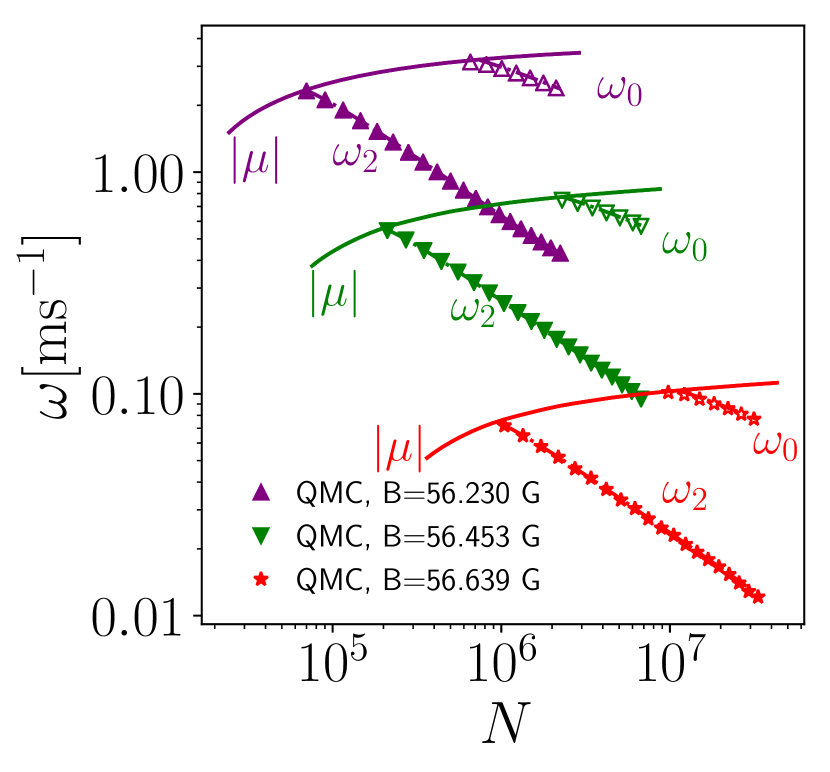
Figure 9: Predictions of the frequency corresponding to the absolute value of the chemical potential $|\mu|$, breathing frequency $\omega_{0}$ and quadropole frequency $\omega_{2}$ as a function of total atom number, using the QMC functionals. Dashed lines are $\omega_{1}=E_{1}/\hbar$ frequencies.

V Summary and outlook

Using a new QMC-based density functional which properly incorporates finite-range effects, we have determined the monopole and quadrupole excitation modes of ³⁹K quantum droplets at the optimal MF+LHY mixture composition. Comparing with the results obtained within the MF+LHY approach, we have found that finite-range effects have a detectable influence on the excitation spectrum, whose study may thus be a promising way to explore physics beyond the LHY correction.

We have shown that introducing the QMC functional into the usual DFT methodology can easily be done, as only minor changes need to be made in the (many) existing Gross-Pitaevskii numerical solvers Antoine and Duboscq (2015); Wittek and Calderaro (2015); Schloss and O’Riordan (2018). This opens the door to using better functionals –based on including quantum effects beyond mean-field– in the current applications of the extended Gross-Pitaevskii approach Astrakharchik and Malomed (2018); Ferioli et al. (2019).

The significant difference between the predictions of QMC and MF+LHY functionals for the excitation spectrum indicates that finite-range effects could show up in other dynamical problems as well. In particular, in droplet-droplet collisions Ferioli et al. (2019), where the actual value of the incompressibility might play a relevant role. A reliable functional might also be useful to study quantum droplet aspects that are currently under study for superfluid ⁴He droplets, as the appearance of quantum turbulence and of bulk and surface vorticity in droplets merging; the equilibrium phase diagram of rotating quantum droplets Ancilotto et al. (2018b); Escartín et al. (2019); O’Connell et al. (2020), and the merging of vortex-hosting quantum droplets. These aspects are at present under investigation. Further improvements in the building of a more accurate QMC functional should consider the inclusion of surface tension effects others that those arising from the quantum kinetic energy term Marín et al. (2005).