KMT-2019-BLG-2073: Fourth Free-Floating-Planet Candidate with $\theta_{\rm E}<10\,\mu{\rm as}$

Abstract

We analyze the very short Einstein timescale ($t_{\rm E}\simeq 7\,{\rm hr}$) event KMT-2019-BLG-2073. Making use of the pronounced finite-source effects generated by the clump-giant source, we measure the Einstein radius $\theta_{\rm E}\simeq 4.8\,\mu{\rm as}$, and so infer a mass $M=59\,M_{\oplus}(\pi_{\rm rel}/16\,\mu{\rm as})^{-1}$, where $\pi_{\rm rel}$ is the lens-source relative parallax. We find no significant evidence for a host of this planetary mass object, though one could be present at sufficiently wide separation. If so, it would be detectable after about 10 years. This is the fourth isolated microlens with a measured Einstein radius $\theta_{\rm E}<10\,\mu{\rm as}$, which we argue is a useful threshold for a “likely free-floating planet (FFP)” candidate. We outline a new approach to constructing a homogeneous sample of giant-star finite-source/point-lens (FSPL) events, within which the subsample of FFP candidates can be statistically analyzed. We illustrate this approach using 2019 KMTNet data and show that there appears to be a large $\theta_{\rm E}$ gap between the two FFP candidates and the 11 other FSPL events. We argue that such sharp features are more identifiable in a sample selected on $\theta_{\rm E}$ compared to the traditional approach of identifying candidates based on short $t_{\rm E}$.

1 Introduction

Characterizing the free-floating planet (FFP) population is the first step in understanding their origins. FFP candidates were originally identified from their short Einstein timescales,

$$t_{\rm E}\equiv{\theta_{\rm E}\over\mu_{\rm rel}};\qquad\theta_{\rm E}\equiv\sqrt{\kappa M\pi_{\rm rel}};\qquad\kappa\equiv{4G\over c^{2}{\rm AU}}\simeq 8.1\,{{\rm mas}\over M_{\odot}},$$ (1)

where $\theta_{\rm E}$ is the Einstein radius, $M$ is the mass of the lens, and $(\pi_{\rm rel},{\mbox{\boldmath$\mu$}}_{\rm rel})$ are the lens-source relative (parallax, proper motion). Sumi et al. (2011) found evidence for a population of low-mass objects from a bump in the timescale distribution at $t_{\rm E}\sim 1\,$day, corresponding to roughly Jupiter mass objects, from their analysis of two years of data from the MOA-II survey. A subsequent analysis of substantially more data from the OGLE-IV survey by Mróz et al. (2017) concluded that there was no such excess of $t_{\rm E}\sim 1\,$day events, but they did find an excess of shorter, $t_{\rm E}\sim 0.2\,$day, events. According to the $t_{\rm E}\propto M^{1/2}$ scaling of Equation (1), this would correspond to roughly Neptune-mass planets.

However, it is difficult to make inferences about the mass of any particular microlens based on the Einstein timescale alone, because this quantity depends on $\pi_{\rm rel}$ and $\mu_{\rm rel}$ as well as the lens mass. That is, at fixed $t_{\rm E}$, the mass scales as $M\propto\mu_{\rm rel}^{2}/\pi_{\rm rel}$ as a function of these unknown quantities. In particular, $\mu_{\rm rel}$ can easily vary by a factor $\sim 5$ for typical lenses, making inferences about individual objects very uncertain. Moreover, in contrast to bound planets with luminous hosts, there is no hope of measuring $\mu_{\rm rel}$ from subsequent high resolution observations for FFPs. Hence, one must adopt a statistical approach to derive conclusions about a putative population that generates excess events as a function of timescale.

A substantial step forward was taken by Mróz et al. (2018, 2019, 2020) when they measured the angular Einstein radii of four short $t_{\rm E}$ events, including three with $\theta_{\rm E}<10\,\mu{\rm as}$, namely OGLE-2012-BLG-1323, OGLE-2019-BLG-0551, and OGLE-2016-BLG-1540, with corresponding Einstein radii $\theta_{\rm E}=(2.37,4.35,9.2)\,\mu{\rm as}$. These measurements were made thanks to the fact that, in each case, the lens transited the source, giving rise to “finite source effects”, i.e., deviations from a standard Paczyński (1986) light curve. These $\theta_{\rm E}$ measurements partially break the three-way degeneracy in Equation (1) by removing $\mu_{\rm rel}$ as an unknown. Hence, for these three lenses, the mass can be estimated

$$M={\theta_{\rm E}^{2}\over\kappa\pi_{\rm rel}}\rightarrow(14,48,217)M_{\oplus}\biggl{(}{\pi_{\rm rel}\over 16\,\mu{\rm as}}\biggr{)}^{-1},$$ (2)

where we have scaled to a typical value of $\pi_{\rm rel}$ for lenses in the Galactic bulge. If the lenses lay in the Galactic disk, the mass estimates would be lower.

The scaling in Equation (2) illustrates that “$\theta_{\rm E}<10\,\mu{\rm as}$” is a qualitative indicator of “good FFP candidate”. That is, at this boundary, a lens would have to have $\pi_{\rm rel}<1\,\mu{\rm as}$ in order to be in the formal brown-dwarf regime, $M>13\,M_{\rm jup}$. Of course, such events (with lens-source distances $D_{LS}\lesssim 10\,$pc) can happen, but they are extremely rare. Thus, the appearance of three FSPL events in the regime $\theta_{\rm E}<10\,\mu{\rm as}$ is strong evidence of a population of FFPs (or wide-orbit planets for which the host does not give rise to any signal in the event).

All three of the sources are giant stars, with angular source radii $\theta_{*}=(11.9,19.5,15.8)\,\mu{\rm as}$. If the sources lie in the bulge at $D_{s}\sim 8\,{\rm kpc}$ (as they almost certainly do based on their kinematics and the relative probability of their being lensed), then these correspond to physical source radii $R_{*}\sim(20,33,27)\,R_{\odot}$. This is not accidental. Accurate measurement of finite-source effects requires many points over the source crossing time, $t_{*}=\theta_{*}/\mu_{\rm rel}$, and the chance of obtaining many measurements is enhanced when $\theta_{*}$ is large. In fact, the sources in these three events are exceptionally large, even for giants.

Here, we report on the discovery of a fourth FFP candidate that satisfies the criterion $\theta_{\rm E}<10\,\mu{\rm as}$, KMT-2019-BLG-2073, with $\theta_{\rm E}=4.8\,\mu{\rm as}$. Like the previous three candidates, the lens magnifies a giant star in the Galactic bulge, in this case with $\theta_{*}=\,5.4\,\mu{\rm as}$.

This discovery prompts us to map out a strategy and carry out the preliminary work for a statistical study of FFP candidates that have $\theta_{\rm E}$ measurements. Such a study, based on $\theta_{\rm E}$, has three major advantages over previous efforts using the $t_{\rm E}$ distribution to characterize the FFP population.

First, as mentioned above it is subject to significantly less ambiguity in the mass of candidates. For a study based on $t_{\rm E}$, the underlying mass distribution will still be convolved with the $\mu_{\rm rel}$ distribution. By contrast, one based on $\theta_{\rm E}$ is independent of the $\mu_{\rm rel}$ distribution.

Second, a distribution based on $\theta_{\rm E}$ will have an intrinsically higher proportion of FFP candidates compared to one based on $t_{\rm E}$. As pointed out by Gould & Yee (2012) in another context, the intrinsic rate of point-lens events that display finite-source effects by any class of objects scales directly with the number density of this class of objects (assuming that all classes of lenses have the same kinematic and physical distribution). That is, the cross section in the rate equation for all events is $2\theta_{\rm E}$ (which scales $\theta_{\rm E}\propto M^{1/2}$), while the cross section in the rate equation for finite-source events is $2\theta_{*}$, which has no mass dependence. Thus, low-mass objects, planets in particular, are favored relative to the general rate by a factor $(M_{\rm planet}/M_{\rm star})^{-1/2}=100[(M_{\rm planet}/M_{\rm Neptune})/(M_{\rm star}/0.5\,M_{\odot})]^{-1/2}$.

Third, the relevant timescale of a search for FSPL events is relatively independent of the lens mass, or more precisely, of the direct observable, $\theta_{\rm E}$. The detection and characterization of an event requires that the relevant timescale be longer than the interval between observations, with the characterization improving with increasing timescale. For FFP events, $t_{\rm E}$ becomes comparable to the cadence of microlensing surveys. So, for a $t_{\rm E}$-based search, it becomes increasingly difficult to detect events as the mass (and so $t_{\rm E}$) decreases. By contrast, an FSPL-based search relies only on $t_{*}$, which is independent of mass and is the lower-limit on the half-width duration of an FSPL event. For example, the Einstein timescale of OGLE-2016-BLG-1928 was only $t_{\rm E}\approx 0.0288\ \mathrm{days}$ whereas the event itself lasted for an order magnitude longer due to finite source effects (Mróz et al., 2020). Hence, to a certain limit (see Section 6), it is no more difficult to detect and characterize small $\theta_{\rm E}$ events than larger ones. As a result, the selection function for a $\theta_{\rm E}$-based study of the FFP population is much simpler than for a $t_{\rm E}$-based study.

Finally, the fact that the known FSPL FFP candidates all have giant sources, leads us to consider a $\theta_{\rm E}$ search restricted to such sources. This empirical observation results, in part, from the fact that the rate at which finite source effects occur is proportional to $\theta_{*}$. Hence, one advantage of focusing on giant sources is that they have a higher proportion of FSPL events relative to smaller sources. However, restricting the search to giant sources also has a number of other practical implications, which we discuss in more detail in Section 6. But first, we turn our attention to KMT-2019-BLG-2073, the inspiration for this search.

2 Observations

KMT-2019-BLG-2073, at (RA, Decl.)_J2000 = (17:49:53.08, $-29$:35:17.30) [$(l,b)=(-0.07,-1.13)$] was announced by the Korea Microlensing Telescope Network (KMTNet, Kim et al. 2016) AlertFinder system (Kim et al., 2018b) as “clear microlensing” at UT 04:41 on 14 August 2019 (HJD^′ = HJD - 2450000 = 8709.70). KMTNet is comprised of three identical 1.6m telescopes with $(2^{\circ}\times 2^{\circ})$ cameras at three sites, Siding Spring Observatory, Australia (KMTA), Cerro Tololo Inter-American Observatory, Chile (KMTC), and South African Astronomical Observatory, South Africa (KMTS). The event lies in the overlap region of KMT fields BLG02 and BLG42, with a combined $I$-band cadence of $\Gamma=4\,{\rm hr}^{-1}$, with every tenth such exposure complemented by one in the $V$ band.

The event, which had an effective duration of only about one day, was essentially over at the time of the alert. Moreover, the first pipeline pySIS light curve (Albrow et al., 2009) was not posted to the KMTNet webpage until about five hours later due to a backlog of newly alerted events. Hence, no followup observations were possible.

Although many dozens of events, including other FSPL events, were actively modeled in real time during the 2019 season by up to a dozen modelers, this event was not. However, the online light curve showed clear deviations that are indicative of finite-source effects in an $A_{\rm max}\sim 2$ event on a cataloged source with dereddened apparent magnitude $I_{0}=14.38$, implying that $\rho\sim\sqrt{A_{\rm max}^{2}-1}/2\sim 1$, and hence $\theta_{\rm E}\sim\theta_{*}\sim 6\,\mu{\rm as}$ (assuming, as proves to be the case, that the source color is similar to the clump). That is, even in the real-time data, this was a very plausible FFP candidate. While this is only one case, it may indicate that there are other FFP candidates that are not being recognized from pipeline data using current human-review and machine-review techniques.

The event was first noticed as a potential FFP candidate in February 2020, during a routine inspection of all events found by the KMTNet EventFinder (Kim et al., 2018a), which included the rediscovery of KMT-2019-BLG-2073. The data were then rereduced using a tender loving care (TLC) implementation of the same pySIS algorithm (Albrow et al., 2009), which is a specific variant of difference image analysis (DIA, Tomaney & Crotts 1996; Alard & Lupton 1998).

3 Light Curve Analysis

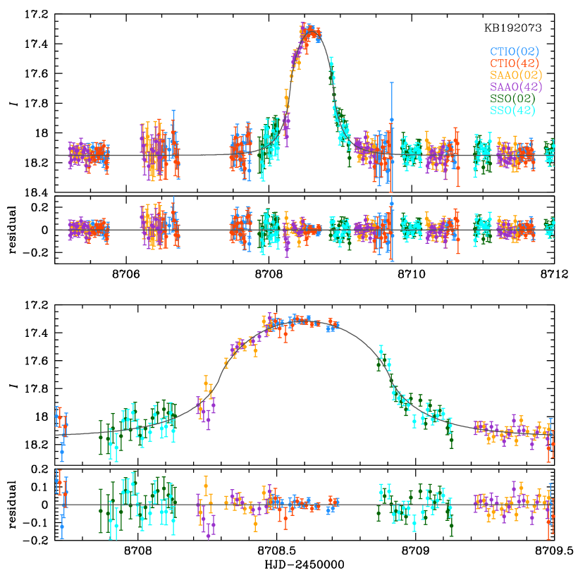
Figure 1: Light curve and model for KMT-2019-BLG-2073, which was observed continuously (weather permitting) at a cadence of $\Gamma=4\,{\rm hr}^{-1}$ from three KMTNet observatories (KMTA, KMTC,KMTS) in two overlapping fields (BLG02, BLG42). The upper panel shows a five-day interval containing the brief event, while the lower panel shows a zoom. In fact the Einstein radius crossing time is only $t_{\rm E}\simeq 0.31$ days, but the event is stretched by pronounced finite-source effects, which enable a measurement of the Einstein radius: $\theta_{\rm E}=4.8\pm 0.2\,\mu{\rm as}$. This implies a lens mass of $M=59\,M_{\oplus}(\pi_{\rm rel}/16\,\mu{\rm as})^{-1}$ where $\pi_{\rm rel}$ is the lens-source relative parallax. This planetary lens has no known host. Each panel also shows residuals.

The light curve appears to be a featureless, symmetric, short-duration bump that is qualitatively consistent with single-lens/single-source (1L1S) microlensing. As mentioned in Section 2, it shows strong deviations from a simple Paczyński (1986) fit, whose geometry is characterized by three parameters $(t_{0},u_{0},t_{\rm E})$, i.e., the time of peak magnification, the impact parameter (scaled to $\theta_{\rm E}$), and the Einstein timescale. These deviations are well explained by adding $\rho=\theta_{*}/\theta_{\rm E}$ as a fourth parameter. In addition, there are two parameters $(f_{s},f_{b})_{i}$ for each observatory $i$ that represent the source and blended flux, respectively. See Figure 1. In deriving this fit, we adopt a linear limb-darkening parameter $\Gamma=0.53$ based on the source typing (clump giant) given in Section 4.

Table 1 shows the results of two fits to the data, one with a free blending parameter $f_{b}$ and the other with fixed $f_{b}=0$. These results show that the free fit is consistent with $f_{b}=0$ at $1\,\sigma$. As discussed by Mróz et al. (2020), the blending fractions of $\eta=f_{b}/f_{\rm base}$ of (apparently) clump-giant sources are bimodal between values close to 0 and 1. Because the result is consistent with $\eta=0$, we will eventually adopt the fixed $f_{b}=0$ solution. Nevertheless, in order to better understand the implications of this choice, we first carefully examine the free-blending solution.

As shown in Table 1, for the free-blending fit, the errors in $t_{\rm E}$ and $\rho$ are 10% and 12%, respectively. However, these are highly anti-correlated, so that the source crossing time $t_{*}\equiv\rho t_{\rm E}$ is measured to better than 4%. The fractional error in $f_{s}$ is even larger, 22%. However, we also show in Table 1, the normalized surface brightness,

$$\hat{S}\equiv{f_{s}\over\rho^{2}}=\pi\theta_{\rm E}^{2}{f_{s}\over\pi\theta_{*}^{2}},$$ (3)

which, like $t_{*}$, has a much smaller fraction error than either of the factors that enter it, i.e., $\sigma(\ln\hat{S})=5\%$. This parameter combination is motivated by the argument of Mróz et al. (2020), who showed that in the limit of $\rho\gg 1$, $\theta_{\rm E}=\theta_{*}/\rho$ is much better determined than either $\theta_{*}$ or $\rho$. The underlying physical reason is that the excess flux due to a lens acting on a very large ($\rightarrow\infty$) source of uniform surface brightness $S$, is just $\Delta F=2\pi\theta_{\rm E}^{2}S$. Hence, if the source color (and so surface brightness) is considered known, then the empirically observed excess flux directly gives the Einstein radius $\theta_{\rm E}$, even if $f_{s}$ (and therefore $\theta_{*}$) and $\rho$ are poorly measured.

In the present case, we are not in the limit $\rho\gg 1$, but the same argument applies reasonably well. That is, if we assume that the source color is known, then $\theta_{*}$ scales with $\sqrt{f_{s}}$ via,

$$\theta_{*}=\sqrt{f_{s}\over f_{s,\rm fid}}\theta_{*,\rm fid},$$ (4)

where $\theta_{*,\rm fid}$ is the value of $\theta_{*}$ at some arbitrarily chosen value of $f_{s,\rm fid}$. Then, from the measurement of $\hat{S}$ (Equation (3)),

$$\theta_{\rm E}={\theta_{*}\over\rho}={\theta_{*,\rm fid}\over\sqrt{f_{s,\rm fid}}}{\sqrt{f_{s}}\over\rho}={\theta_{*,\rm fid}\over\sqrt{f_{s,\rm fid}}}\hat{S}.$$ (5)

The source flux $f_{s}$ is consistent with the baseline flux $f_{\rm base}\equiv f_{s}+f_{b}$ at $\sim 0.4\,\sigma$ (keeping in mind that the errors in $f_{s}$ and $f_{b}$ are almost perfectly anti-correlated). Given that the source lies in or near the clump, it is therefore quite plausible that $f_{s}$ is essentially equal to $f_{\rm base}$, and that the apparent difference is due to modest statistical errors. As we have just shown, this would make essentially no difference for the $\theta_{\rm E}$ determination, which is of primary interest. However, it would affect the proper-motion estimate, which is also of importance. That is, $\mu_{\rm rel}=\theta_{\rm E}/t_{\rm E}=(\theta_{\rm E}/t_{*})\rho$. Because $\theta_{\rm E}$ and $t_{*}$ are nearly invariant, $\mu_{\rm rel}\propto\rho$. Thus, the principal difference between the $f_{b}=0$ and free $f_{b}$ solutions is that that latter have an additional fractional error in $\mu_{\rm rel}$ equal to that of $\rho$, i.e., $\sim 12\%$. As stated above, we adopt the $f_{b}=0$ solution because of the low prior probability of intermediate blending parameter $\eta$. Nevertheless, for applications that depend sensitively on the proper motion (e.g., delay time until future high-resolution imaging), this potential source of proper-motion uncertainty should be given due weight.

4 Color Magnitude Diagram

4.1 Overview

For essentially all microlensing events, the main goal of the color-magnitude diagram (CMD) analysis is to measure $\theta_{*}$ and so $\theta_{\rm E}=\theta_{*}/\rho$ and $\mu_{\rm rel}=\theta_{\rm E}/t_{\rm E}$. This is also true in the present case, but with somewhat different emphasis. First, the $\theta_{\rm E}$ measurement is of overarching importance. Second, in contrast to typical events, this measurement depends almost entirely on the source color (see Equation (5) and Table 1). Third, this source color cannot be reliably measured from the light curve. Thus, most of this section is focused on quantifying the uncertainty of the source color and the impact of this uncertainty on $\theta_{\rm E}$ (and also $\mu_{\rm rel}$). However, in order not to distract the reader with the details of this investigation, we note at the outset that Equation (6), below, gives our best estimate of the value and statistical error in $\theta_{\rm E}$, and that the probability of significant systematic deviation from this result is small.

4.2 Source Color Not Measured From Event

In order to estimate $\theta_{\rm E}$, we find the source’s position relative to the clump on the CMD (Yoo et al., 2004). Normally, the source color would be derived from observations of the event in two different bands, either by fitting both light curves to the same model or by regression. However, this is not possible in the present case. Despite the brevity of the event, there are four $V$-band measurements over the peak from KMTC. However, the extinction (estimated below at $A_{I}\sim 3.7$) and intrinsically red source imply that the $V$-band difference fluxes at peak correspond to a roughly $V\sim 22$ “difference star”. This was too faint for the observations to yield a measurement of useful precision.

4.3 Analysis Assuming That Source = “Baseline Object”

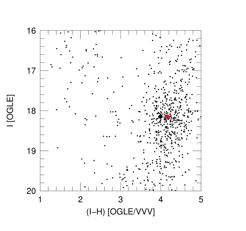
Figure 2: Calibrated $I$ vs $(I-H)$ CMD for KMT-2019-BLG-2073 derived by matching OGLE-III $I$ and VVV $H$ photometry. The black point shows the position of the “baseline object” derived from these catalogs, while the red point shows the clump centroid. We derive the source radius $\theta_{*}$ under the assumption that it is unblended (source = baseline) and under the assumption that it is blended. In either case, $\theta_{*}\sim 5\,\mu{\rm as}$, implying that the Einstein radius is $\theta_{\rm E}\sim 5\,\mu{\rm as}$ as well.

Instead, we evaluate the color of the “baseline object” using archival $I$-band photometry from the OGLE-III survey (Szymański et al., 2011) matched to archival $H$-band photometry from the VVV survey (Minniti et al., 2017) to make a first estimate of the source color. See Figure 2.

There are two reasons why this approach is appropriate. First, we find that the source position, as determined from astrometry on the difference images from the peak night at KMTC, is aligned within 0.063 pixels (25 mas) of position of the baseline object on the reference image. Hence, if any star other than the source contributes significantly to the baseline object, it must be very closely aligned with the source. While this could certainly be the case for a star associated with the event (i.e., a companion to the source or a host of the lens), it is very improbable for a random interloper. That is, the surface density of stars that are, e.g., 10% as bright as a clump giant, is low, so that the probability of one falling within a few tens of mas of a randomly chosen location is extremely low.

Second, the flux parameters shown in Table 1 for free blending imply that most of the baseline-object flux is due to the source, and the baseline flux is consistent with all being due to the source.

Hence we adopt this $f_{b}=0$ assumption to make our first estimate for the source color and magnitude. According to Figure 2, the baseline object (and hence source, under this hypothesis) is separated from the clump by $\Delta[(I-H),I]=(-0.16,0.00)\pm(0.02,0.03)$. Using the dereddened clump position $[(V-I),I]_{\rm clump,0}=(1.06,14.45)$ (Bensby et al., 2013; Nataf et al., 2013) and the color-color relations of Bessell & Brett (1988), this implies $\Delta[(V-I),I]=(-0.12,0.00)\pm(0.02,0.03)$ and so $[(V-I),I]_{s,0}=(0.94,14.45)\pm(0.02,0.03)$. Then, again using the color-color relations of Bessell & Brett (1988) as well as the color/surface-brightness relations of Kervella et al. (2004), we obtain,

$$\theta_{*}=5.43\pm 0.17\,\mu{\rm as};\quad\theta_{\rm E}=4.77\pm 0.19\,\mu{\rm as};\quad\mu_{\rm rel}=6.41\pm 0.24\,{\rm mas}\,{\rm yr}^{-1};\quad(f_{b}=0),$$ (6)

where we have employed the “$f_{b}=0$” solution from Table 1, as is appropriate for these assumptions.

4.4 Possibility That Source $\not=$ “Baseline Object”

We now consider the possibility that some of the baseline flux is due to another star, i.e., other than the microlensed source. As we noted above, the close astrometric alignment of the source with the baseline object argues against significant light coming from an ambient star. It is also unlikely that substantial additional light is contributed by a companion to the source because it would be subject to the same heavy extinction as the source. Moreover, the main possibility would be a subgiant companion because giant companions would be extraordinarily rare and main-sequence companions would contribute hardly any light. In this context, we note that the subgiant would contribute a modest amount of flux, which would be of similar color to the baseline object. Hence, by the argument given in Section 3, the Einstein-radius estimate would be essentially the same as the $\theta_{\rm E}=4.8\,\mu{\rm as}$ estimate given in Equation (6), while the proper motion $\mu_{\rm rel}\propto\rho$ would be lower by of order 15%. Because this solution is qualitatively the same for $\mu_{\rm rel}$ and quantitatively nearly identical for $\theta_{\rm E}$, we do not pursue it in detail.

Instead, we examine the possibility that significant blended light comes from a (putative) host of the lens. We will derive constraints on this scenario in Section 5, but for present purposes, we simply note that if a host lay more than a few mas away, it would not have any perceptible impact on the light curve, and if it were less than 50 mas, it would not violate the astrometric constraints. Thus, this possibility cannot be ruled out based on existing observations.

However, if the putative host lay behind the majority of the dust, it would face the same arguments as were given above for a companion to the source. On the other hand, if the lens were relatively nearby to the Sun, it could contribute substantial light both because of its proximity and because it was less extincted than the source. In this case, it could also contribute significant $V$-band light, which would render the source redder than the baseline object.

From the standpoint of exploring a range of possibilities, this is the main feature of interest because, according to the argument of Mróz et al. (2020), only a change in the source color can alter the estimate of $\theta_{\rm E}$. To be concrete, we assume that $-8\%\pm 22\%$ of the $I$-band light is due to the blend (see Table 1) and that the source color is that of the clump, $(V-I)_{0}=1.06\pm 0.10$, which is the most likely color in this region of the CMD. This could in principle be achieved if the lens (and so lens companion) lay in theforeground, i.e., in front of a substantial fraction of the dust, and so were $\Delta(V-I)\sim-1\,$mag bluer than the source. In any case, it is highly unlikely that the source can be substantially redder than this range because this would put it in a highly underpopulated region of the CMD.

From Equation (5), $\theta_{\rm E}$ is the product of two terms, the first depending only on the source color and second being $\hat{S}$. The mean value of the latter does not change for free blending, although its uncertainty becomes larger, i.e., 5%. When the color is increased from $(V-I)_{0}=0.94$ to $1.06\pm 0.10$, this increases the color term in Equation (5) by $14\%\pm 11\%$. Hence, under the assumption that the relatively blue color (for a clump star) of the baseline object is due to “contamination” by the host of the lens (or a companion of the host), $\theta_{\rm E}$ would be larger by $20\%\pm 12\%$, i.e., $5.72\pm 0.57\,\mu{\rm as}$. In addition, if, e.g., 10% of the $I$-band flux were due to the putative host system, then the proper-motion estimate would be reduced by 5% relative to Equation (6).

We conclude that Equation (6) gives the best estimate of $\theta_{\rm E}$ and $\mu_{\rm rel}$, but even if the baseline object includes substantial blue light due to a putative host of the lens that lies in front of much of the dust, the estimates of $\theta_{\rm E}$ and $\mu_{\rm rel}$ do not qualitatively change.

4.5 Comparison of KMT-2019-BLG-2073 and OGLE-2019-BLG-0551

Finally, it is worthwhile to compare how the parameter estimates of KMT-2019-BLG-2073 and OGLE-2019-BLG-0551 (Mróz et al., 2020) are affected by the introduction of free-blending. For OGLE-2019-BLG-0551, the color was measured directly from the light curve. Therefore, the assumption of fixed color, employed by Mróz et al. (2020) in their derivation of the invariance of $\theta_{\rm E}$, was fully justified. On the other hand, the light curve provided only very weak constraints on $f_{s}$ (equivalently, $I_{s}$). Therefore, in their Table 1, $\theta_{\rm E}$ is nearly identical between the two models, whereas $\mu_{\rm rel}\propto\sqrt{f_{s}}$ is much smaller for the free-blend case. In addition, the fact that the measured color of the event was the same as the color of the baseline object provided strong evidence of low blending (although this was not explicitly used in the mathematical analysis).

By contrast, for KMT-2019-BLG-2073, $f_{s}$ is well-measured (and is close to $f_{\rm base}$), while there is no measurement of the source color per se (only of the baseline object). Hence, the Mróz et al. (2020) argument for invariance of $\theta_{\rm E}$ cannot be used directly, but must be generalized to Equation (5), which includes a color term. The color (and hence color term) is constrained partly by the morphology of the CMD and partly by the fact that $f_{s}$ is measured from the event to be similar to $f_{\rm base}$. As a result, the difference in the values of $\theta_{\rm E}$ are larger for KMT-2019-BLG-2073 than OGLE-2019-BLG-0551, while those of $\mu_{\rm rel}$ are smaller.

5 Search for a Host

Based on its light curve, KMT-2019-BLG-2073 appears to be an isolated lens of very low mass, i.e., an FFP candidate. However, if it were orbiting a star at sufficiently wide separation, then this host would leave only a weak trace of its existence, or perhaps no trace at all. In this section, we search for such weak traces and characterize the separations that we are able to probe.

In our search, we consider models with seven parameters $(t_{0},u_{0},t_{\rm E},\rho,s,q,\alpha)$. The first four are similar to our 1L1S search, except that $(u_{0},t_{\rm E},\rho)$ are all normalized to the Einstein radius of the combined (binary) lens, which is larger than the FFP Einstein ring by a factor $\sqrt{q+1}$, where $q>1$ is the host/planet mass ratio. Then $s$ is the projected host-planet separation scaled to the host+planet Einstein radius, and $\alpha$ is the angle of the lens-source trajectory relative to the host-planet axis. We place the planetary caustic at the center of our coordinate system, so that $u_{0}\simeq 0$ and $t_{0}$ is similar to the value listed in Table 1. We initially conduct a grid search with $(s,q)$ held fixed and with $\alpha$ seeded at six positions drawn from the unit circle. We include two years (2018+2019) of data in order to suppress false signals due to low-level source variability of the giant source. See Mróz et al. (2020) for an alternate approach.

We find no 2L1S models with significant $\chi^{2}$ improvement. More specifically, after seeding a new fit that is free in all seven parameters with the best grid point, we find a shallow minimum at $(s,q,\alpha)=(53,246,12.5^{\circ})$, with $\Delta\chi^{2}=-6.20$ relative to the FSPL ($f_{b}=0$) fit for the same two-year data set and for four additional degrees of freedom $(s,q,\alpha,f_{b})$. Even if one were to assume perfect Gaussian statistics (which is certainly not permissible for microlensing data), this would have a significance $p=(1+\Delta\chi^{2}/2)\exp(-\Delta\chi^{2}/2)=18\%$, which is not significant.

Given that there is no significant evidence for the host in the microlensing light curve, we work to place limits on possible hosts by applying the Gaudi & Sackett (2000) method to the full 2018-2019 KMT light curves. As we show below, this method yields overly strong constraints on hosts because of low-level variability of the source. Nevertheless it yields important insights into the real limits, which then serve to guide an analytic estimate of the limits. We implement this method by conducting a three-dimensional (3-D) $(s,q,\alpha)$ grid search in order to put upper limits on the presence of a host. We again seed the remaining parameters at the FSPL values from Table 1, The grid is equally spaced in $\log q$ over $1<q<10^{6}$, equally spaced in $\log s$ over $1<s<100$, and uniformly spaced in $\alpha$ in $10^{\circ}$ steps.

We find that the constraints derived from this approach are too strong, due to low-level variability of the source. For example, the model $(s,q,\alpha)=(10,100,90^{\circ})$ is nominally excluded at $\Delta\chi^{2}=14$ with $\Delta\chi^{2}=10$ coming from the 2018 baseline year. However, close inspection of the 2L1S and 1L1S models shows that they only differ by $7\times 10^{-5}$ mag during 2018. There are about $N=6000$ points in 2018, with overall median error $\sigma=0.032$ mag. Hence, the baseline can only be measured to a precision $\sigma/\sqrt{N}=4\times 10^{-4}$ mag, so it is clearly impossible to distinguish these two solutions using these data. The reason for the formally high $\Delta\chi^{2}$ is that the data are about 0.01 mag higher than either model (due to source variability). This is a standard systematic effect, which improperly augments the $\chi^{2}$ difference by a factor $2\times(0.01)/(7\times 10^{-5})\sim 300$. Hence, we cannot blindly apply this approach.

However, studying the models that are generated by this approach, we find that for each $(s,q)$ in the regime $q>10$, the $\alpha=90^{\circ}$ model is the most weakly constrained. For all of these models, the constraints come from a long low-amplitude “bump”, which is not seen in the data. When $\alpha=90^{\circ}$, this bump has equal amplitude on either side of the planetary spike. At any other $\alpha$ it is higher on one side or the other, which only increases its tension with the data. Therefore, we can restrict attention to the 2-D parameter space $(s,q,\alpha=90^{\circ})$. We also note that between the two potential features that are due to a distant host, i.e., the long bump and the small caustic at the position of the planet, only the first induces significant changes in the lightcurve.

In this $\alpha=90^{\circ}$ geometry and for $s\gg 1$, the separation of the source and host is given by $u=\sqrt{s^{2}+(t-t0)^{2}/qt_{\rm E}^{2}}$ where $t_{\rm E}=0.27\,$days is the Einstein timescale of the FFP solution. And the excess magnification due to the distant host is well approximated by $\Delta A=2/u^{4}$. Hence, the FWHM of the bump is given by $\Delta t_{\rm FWHM}=2(\sqrt{2^{1/2}-1}s\sqrt{q}t_{\rm E}=1.3s\sqrt{q}t_{\rm E}$. That is,

$$\Delta t_{\rm FWHM}=78(s/7)\sqrt{q/1000}\,{\rm day}.$$ (7)

Hence, for $q<1000$, both the bump and the adjacent baseline are contained within the 2019 data, which is relatively unaffected by the long term variability. Taking account of the analytic form of the bump and the photometric errors, we find that for a given $q$ in this regime, $s$ is constrained to be

$$s>7\biggl{(}{q\over 1000}\biggr{)}^{1/8};\qquad 1<\log q<3.3$$ (8)

On the other hand for $q>10000$, the bump extends over most of the 2019 season. We must therefore rely on the 2018 baseline measurement, which can only be constrained to within 0.01 mag due to source variability. This implies that the limit is $s>3.3$. That is, for this limiting value $u=s-1/s\sim 3$ so that $A-1=0.017$, which can clearly be distinguished from the baseline, even with the uncertainty due to variability. That is,

$$s>3.3\qquad\log q>4.0$$ (9)

Finally, in the intermediate regime, as $q$ rises, the limiting value of $s$ must fall $s\propto q^{1/2}$ in order to keep the bump confined to the 2019 season (according to Equation (7)),

$$s>7.6\biggl{(}{q\over 2000}\biggr{)}^{-1/2};\qquad 3.3<\log q<4.0.$$ (10)

Finally, we note that in the regime $q<10$ (which would correspond to an exotic FFP planet-moon scenario) the caustic plays a dominant role and rules out all $s$ in the ranges considered above.

To gain intuition about the physical implications of these constraints, we consider two test cases. Suppose that the lens corresponds to a Jupiter-mass planet. Then, a $1\,M_{\odot}$ host would have $q=10^{3}$. The physical Einstein radius for such a system is given by

$$r_{\rm E}=\frac{\theta_{\rm E,p}D_{\rm L}}{q}$$ (11)

where $\theta_{\rm E,p}$ is the angular Einstein radius of the planet, which is $4.8\mu$as in this case. Equation (2) gives $\pi_{\rm rel}=2.8\ \mu$as and $D_{\rm L}=7.8\$ kpc (for $D_{\rm S}=8$ kpc). Equation (8) indicates a limit of $s>7$, which corresponds to a limit of $a_{\perp}=sr_{\rm E}>8.3$ au. Alternatively, consider the case of a Neptune mass ratio $q=2\times 10^{4}$ and an $0.3\,M_{\odot}$ host. In that case, the limit is given by Equation (9), so $s>3.3$ or $a_{\perp}>7.1$ au. While these constraints are significant, they would not rule out, e.g., a Neptune analog. We discuss how to place additional constraints on the presence (or absence) of a host star in Section 7.2.

6 Outline of Statistical Approach to Isolated-Lens Finite-Source Events

The detection of two isolated lenses with FFP-class ($\theta_{\rm E}<10\mu{\rm as}$) Einstein radii in 2019 suggests that a statistically meaningful number of such lenses could exist in four years of KMTNet survey data. This motivates us to develop a statistical procedure that can guide future searches, including both archival and prospective data. Here we present the motivations for our approach, describe a specific implementation, and then apply this implementation to the 2019 KMT database.

We strongly emphasize that even though this implementation will yield a statistically well-defined sample, the 2019 sample alone absolutely cannot be used to derive statistical inferences about FFPs. This is because, as stated above, we were motivated to undertake this study due to the detection of two FFP-class events. Hence our study is, by definition, critically impacted by publication bias. Nevertheless, because the sample is statistically well-defined, it will allow us to address possible issues in the construction of a larger, unbiased, statistical sample.

Thus, the primary purpose of this work is to establish the methodology for carrying out a statistical study of FFP candidates using the $\theta_{\rm E}$ distribution. In future work (e.g. KB172820 in Ryu et al., 2021), we will extend this procedure to the full (unbiased) sample of KMTNet events from which statistical conclusions can be drawn.

6.1 Motivation

Our basic goal is to assemble a homogeneous and complete sample of 1L1S events with secure finite source effects, i.e., FSPL events, in order to characterize the population of FFPs. As mentioned in Section 1, the focus on FSPL events has several major advantages over trying to characterize the population based on $t_{\rm E}$ alone. If, for the moment, we identify such events as those with $z_{0}\equiv u_{0}/\rho\leq 1$, then their underlying cross section is $2\theta_{*}$, independent of the mass, distance, or transverse velocity of the lens. Hence, (under the assumption that the distance and proper-motion distributions of the lenses is independent of the lens mass $M$), each subclass of lenses (classified by, e.g., their mass) will contribute to this homogeneous sample in direct proportion to their number density. This is an advantage over the $t_{\rm E}$ distribution, to which lenses contribute in proportion both to their number density and to (the square-root of) their mass.

The second advantage is that, for each member of the sample, the measurement of $\theta_{\rm E}$ will imply a probability distribution for the lens mass that is directly related to the Galactic-model distribution of lens-source relative parallax, $\pi_{\rm rel}$,

$$M={\theta_{\rm E}^{2}\over\kappa\pi_{\rm rel}}.$$ (12)

Thus a $\theta_{\rm E}$-based sample is subject to much less uncertainty than a $t_{\rm E}$-based sample, for which $M\propto\mu_{\rm rel}^{2}/\pi_{\rm rel}$. Furthermore, there does not appear to be a large population of free-floating Jupiters, but rather the FFP population, should it exist, must peak at lower masses. Hence, because the distribution of $\pi_{\rm rel}^{-1}$ is relatively compact, while the peaks of the planetary and stellar mass functions are separated by several orders of magnitude, the observed distribution of $\theta_{\rm E}^{2}$ should also be bimodal and thus, can directly constrain the relative frequency of stars and FFPs.

However, the key to being able to make a statistical statement lies in having a well-defined and statistically robust sample of events with $\theta_{\rm E}$ measurements. As usual, the devil is in the details of the selection function. For “complete selection”, all of the specified class of FSPL events must be identified as microlensing candidates (not necessarily immediately identified as FSPL events), and must be closely examined with high-quality reductions for the solid detection of finite-source effects. That is, they must be selected independent of $\theta_{\rm E}$, or at least with smoothly varying and reasonably well known selection as a function of $\theta_{\rm E}$.

6.1.1 Advantages of Giant Sources

These goals are strongly aided by restricting the investigation to giant-star sources. There are a number of reasons for this.

First, the fraction of events with underlying (not necessarily detected) finite-source effects is directly proportional to $\theta_{*}$, which is of order 10 times larger for giants than dwarfs. Thus, it is more efficient to search for FSPL events with giant sources.

Second, the machine classification of source-star characteristics is much more accurate for giant sources because they are typically much less blended. The first implication of this is that it is easier to create a well-defined sample of giant sources. In addition, for lower-mass lenses, for which FSPL events are typically fainter at peak, so that the true position centroid of dwarf sources is much less likely to be recovered by automated means. Because the accuracy of the centroid affects the quality of the photometry, finite-source event candidates can be more reliably identified for giant sources.

Third, because giant sources are brighter, they tend to have higher-precision photometry simply due to improved photon noise. As just mentioned, better photometry improves the detectability (and characterization) of finite-source effects.

Fourth, the number of giant-source events is an order of magnitude smaller, which makes for a more tractable sample. In addition, it is more likely to be complete than a larger sample. For example, considering dwarf-source events creates an order of magnitude more work in careful vetting of candidates, while we expect a smaller fraction of them to exhibit finite source effects, and thus increases the chance that a significant fraction of the finite-source events will be missed.

Fifth, because giant sources have a larger $\theta_{*}$, they also have a longer $t_{*}$ at fixed $\mu_{\rm rel}$, which has a number of consequences. First, the longer duration means that more observations are taken that characterize the event at fixed cadence. This makes the giant source, FSPL events both better characterized and easier to detect than either dwarf source FSPL or FFP-candidate PSPL events. By contrast, $t_{*}\sim 1\,$hr for dwarf stars, whereas the cadence of the survey fields ranges from $4\,{\rm hr}^{-1}$ to $1\,{\rm day}^{-1}$ or less. As a consequence, the data probing the finite-source effects are many times fewer (and often completely absent) for dwarf sources.

The second, third, and fourth points all make the selection function simpler and also easier to accurately model for giant sources compared to dwarfs.

6.1.2 Limits of Giant Sources

The fundamental limit of a giant-source FSPL-based search for FFPs is that at sufficiently small masses, the ratio $\rho\equiv\theta_{*}/\theta_{\rm E}$ rises well above unity, which has two major consequences.

First, when $\rho>1$, the excess magnification (Maeder, 1973; Riffeser et al., 2006; Agol, 2003),

$$A-1=\sqrt{1+{4\over\rho^{2}}}-1,$$ (13)

scales as

$$A-1=\rightarrow{2\over\rho^{2}}={2\kappa\pi_{\rm rel}\over\theta_{*}^{2}}M.$$ (14)

Thus, the photometric and systematic noise and/or the level of source variability (as well as the larger $\theta_{*}$) set the fundamental limit on the mass that can be detected.

Second, the events may no longer look like standard Paczyński (1986) light curves. Hence, they may be missed by an event-detection algorithm designed to detect Paczyński (1986) curves, such as the one used in the standard KMTNet pipeline. While this practical problem of recognition can be ameliorated because it is known, it will need to be studied in detail (see also Section 6.2.2).

Finally, we note that because giant sources are bright, it will be difficult to impossible to detect excess light due to a dwarf host star (should one exist) while the source and lens are still super-posed. While this difficulty can be overcome simply by waiting for the lens and source to separate sufficiently far that they can be resolved, the wait time can be quite long. See Section 7.

Hence, while dwarf sources do have some advantages, including sensitivity to FFPs of substantially smaller $\theta_{\rm E}$ (and so mass $M$), it is premature to include them in an initial investigation, i.e., before giant-source events have been thoroughly investigated. Thus, our overall approach is to identify giant-source-star candidates automatically, and then to vet these by detailed individual investigation.

6.2 Specific Implementation

We present a specific implementation of a FSPL search of giant sources based on KMTNet data. In principle, the same general principles outlined in Section 6.1 could be applied to more complex data sets, involving, for example, several microlensing surveys. However, this would significantly increase the complexity of the search process, as well as modeling the selection function. Nevertheless, such an approach could be adopted at a later time.

Each event is selected for further investigation based on the four catalog parameters: $I_{s}$, $u_{0}$, $t_{\rm E}$ and $A_{I}$. The first three are the source magnitude, the impact parameter and the Einstein timescale, all derived from the pipeline PSPL fit. The last is the $I$-band extinction, which is estimated as $A_{I}=7A_{K}$ where $A_{K}$ comes from Gonzalez et al. (2012). We determine $I_{s}=28-2.5\log(f_{s})$, where $f_{s}$ is the source flux in KMTC instrumental (ADU) units. We find from extended practice that this is roughly calibrated, within about 0.1 mag. For the case of catalog values $u_{0}<0.001$, we adopt $u_{0}=0.001$. Our selection is based on two criteria, which we first list and then motivate:

1. (1) $I_{s,0}<16$; $I_{s,0}\equiv I_{s}-A_{I}$

2. (2) $\mu_{\rm thresh}>1\,{\rm mas}\,{\rm yr}^{-1}$;  $\mu_{\rm thresh}\equiv\theta_{*,\rm est}/t_{\rm eff}$;  $\theta_{*,\rm est}\equiv 3\times 10^{(16-I_{s,0})/5}\,\mu{\rm as}$,

where $t_{\rm eff}\equiv u_{0}t_{\rm E}$.

Criterion (1) is simply that the source is a giant (i.e., it has reached the base of the giant branch in its evolution, which is roughly 1.5 mag below the clump). In principle, stars satisfying this criterion could be foreground main-sequence stars. However, if so, these would be eliminated at a later stage.

Criterion (2) is more complex. The overall goal is to eliminate the great majority of giant-source events from consideration, while still preserving essentially all those with FSPL effects and proper motions $\mu_{\rm rel}\gtrsim 1\,{\rm mas}\,{\rm yr}^{-1}$. Because a very small fraction of microlensing events have $\mu_{\rm rel}<1\,{\rm mas}\,{\rm yr}^{-1}$, the overwhelming majority of FSPL events will survive Criterion (2). Specifically, the underlying idea is that $\mu_{\rm thresh}$ would be the estimated lens-source relative proper motion for the case $z_{0}\equiv u_{0}/\rho=1$. We note first that $\mu=\theta_{*}/t_{*}=\theta_{*}(u_{0}/\rho)/(u_{0}t_{\rm E})=z_{0}\theta_{*}/t_{\rm eff}$. Therefore, $\mu=z_{0}\mu_{\rm thresh}(\theta_{*}/\theta_{*,\rm est})$. Hence, if finite source effects are detectable, then $z_{0}\lesssim 1$, and thus events that fail Criterion (2) would have $\mu\lesssim(\theta_{*}/\theta_{*,\rm est})\,{\rm mas}\,{\rm yr}^{-1}$. The estimate of $\theta_{*}$ is based on the assumption that the source has approximately the color of the clump. If this is approximately correct, then any event with detectable finite source effects that failed criterion (2) would have proper motion $\mu\lesssim 1\,{\rm mas}\,{\rm yr}^{-1}$. Such events are very rare. For a very small fraction of sources, the source may prove to be substantially redder than the clump, in which case, it could be, e.g., that $\theta_{*}\sim 2\theta_{*,\rm est}$. Then some events with proper motions as high as $\mu\sim 2\,{\rm mas}\,{\rm yr}^{-1}$ could be eliminated automatically, i.e., prior to human review. These are also relatively rare. In any event, this is a well defined, objective criterion. Hence it eliminates events in a deterministic way that can be modeled, if necessary. The purpose of this criterion is to avoid detailed investigations of events with very low probability of having detectable finite-source effects. We will examine the efficacy of the “$1\,{\rm mas}\,{\rm yr}^{-1}$” boundary on selection in Section 6.3. Finally, as noted above, the fact that events with $z_{0}\lesssim 1$ will generally have detectable finite-source effects implies that events with $\mu_{\rm rel}\lesssim\mu_{\rm thresh}$ will have such effects. This means that events with $\mu_{\rm thresh}\gtrsim 7\,{\rm mas}\,{\rm yr}^{-1}$ are excellent FSPL candidates because most microlensing events have proper motions below this threshold. We will specifically test this idea in Section 6.3.

After an event is selected, it is fit both with (FSPL) and without (PSPL) finite-source effects using the final pipeline pySIS reductions, and the $\Delta\chi^{2}=\chi^{2}({\rm PSPL})-\chi^{2}({\rm FSPL})$ is noted. If $\Delta\chi^{2}>15$, then it is accepted as a FSPL event, and if $\Delta\chi^{2}<3$, then it is rejected. For the remaining few cases, we made TLC re-reductions. Reanalysis then decisively resolved into FSPL ($\Delta\chi^{2}>20$) or PSPL ($\Delta\chi^{2}<3$) for all of these events.

6.2.1 AlertFinder and EventFinder Events

We begin by considering all KMT events discovered during the 2019 season, either by the KMT AlertFinder (Kim et al., 2018b) in real time or the KMT EventFinder (Kim et al., 2018a) in post-season analysis. Comparison of these two samples shows that 581 AlertFinder events were not recovered by the EventFinder. While many of these were spurious or very low-quality events, many others are clearly real, and therefore were missed either because they were excluded by the automatic selection of candidates or were misclassified as “not microlensing” by the operator.

6.2.2 Supplemental Search

To test for (and possibly find) additional FSPL giant-star events that were missed by both AlertFinder and EventFinder, we conduct an additional search based on a modified version of EventFinder. Although, we will apply this search to the 2019 sample, we did not expect (and do not find, see below) many new FSPL events in the 2019 data. Rather, this supplemental search was created in the context of the long term goal of creating a homogeneous sample from four years of survey data, for which the original search algorithms evolved over time.

Hence, in order to both motivate and explain this search, we very briefly review the key features of EventFinder and its evolution. All light curves are modeled by a grid of several thousand 2-parameter ($t_{0},t_{\rm eff}$) Gould (1996) models that are restricted to a $|t-t_{0}|<5\,t_{\rm eff}$ baseline. The $\Delta\chi^{2}$ difference between this fit and a constant model is noted, and the model with the highest such $\Delta\chi^{2}$ is selected for this event. If this model survives the elimination of the highest $\Delta\chi^{2}$ point from each observatory, and if it exceeds a certain threshold $\Delta\chi^{2}_{\rm gould}>\Delta\chi^{2}_{\rm gould,min}$, it is written to a file.

Before discussing how this file is further processed, it is important to note that beginning “halfway” through the 2017 EventFinder analysis, this procedure was modified to add a second step. Events that pass the $\Delta\chi^{2}_{\rm gould}$threshold are fitted to a 3-parameter Paczyński (1986) model, and must similarly exceed a $\Delta\chi^{2}_{\rm paczynski}>\Delta\chi^{2}_{\rm paczynski,min}$ threshold. At first sight this seems more restrictive, but for 2015-2017a, $\Delta\chi^{2}_{\rm gould,min}=1000$, whereas for 2017b-2019, $\Delta\chi^{2}_{\rm gould,min}=400$ and $\Delta\chi^{2}_{\rm paczynski,min}=500$. The additional Paczyński test had the effect of finding lower-signal events while at the same time eliminating a much larger fraction of low-signal spurious candidates that would have required manual rejection by the operator. This also enabled the search to include events with effective timescales $t_{\rm eff}\geq(3/4)^{4}(=0.3164)\,$days, whereas the previous approach was limited to $t_{\rm eff}\geq 1.0\,$day.

The next step is to group similar candidates (as determined by their values of $t_{0}$, $t_{\rm eff}$ and angular position) into groups by a friends-of-friends algorithm. Only the “group leader” (as determined by $\Delta\chi^{2}$) is further considered. This “group leader” is first vetted against a list of known variables and artifacts, and, if it passes, it is shown to the operator.

For the modified EventFinder, we first restrict attention to potential giant sources, defined by $I_{\rm cat}-A_{I}<16.2$, where $I_{\rm cat}$ is the input-catalog “$I$-band” magnitude. Wherever possible, the input catalog is derived from the OGLE-III star catalog (Szymański et al., 2011), which is on the standard Cousins system. Nearly all the remaining catalog entries (about 40%) are derived from the Schlafly et al. (2018) catalog based on DECam data. For these cases, $I_{\rm cat}$ is the catalog value of the SDSS $i$ magnitude. This value is similar to Cousins $I$ for low- or moderately-extincted red giants, but is a few tenths higher (“fainter”) for heavily extincted giants because the SDSS $i$ bandpass is bluer than Cousins $I$. Hence, this could in principle reject some sources that have $I<16$. However, we will show in Section 6.3 that this is a small effect.

Finally, a small fraction of catalog entries that lie in regions not covered by either the OGLE-III or DECam catalogs derive from DoPhot (Schechter et al., 1993) photometry of KMT images. This photometry is aligned to the OGLE-III catalog to within about 0.1 mag and so is on the Cousins scale.

In addition to restricting the catalog stars to giants, we also restrict the models to those with effective timescales of $t_{\rm eff}<5\,$days. This is a conservative cut because most longer $t_{\rm eff}$ events would be rejected by Criterion (2) above. Moreover, those giant-source events that fail this criterion would be very obvious candidates in the regular EventFinder search and so would be unlikely to be missed.

The giant catalog stars selected in this way are then subjected to a Gould (1996) search with $\Delta\chi^{2}_{\rm gould,min}=1000$ and are not subjected to further Paczyński (1986) vetting. In this sense, the search resembles those from 2015-2017a. This feature will eventually enable reasonably homogeneous integration of 2016-2017a EventFinder searches into a full statistical search at a later time. However, in contrast to these early searches, it is carried out for effective timescales $t_{\rm eff}\geq 0.3164\,$days rather than 1.0 day.

Finally, to enhance the operator’s ability to spot non-standard events, in particular those with very large finite-source effects, each event is displayed with three fitting panels (for “$u_{0}=0$”, “$u_{0}=1$”, and “Pacyński” fits) rather than one panel (for best of “$u_{0}=0$” and “$u_{0}=1$” fits). Such multiple displays would be of little benefit for relatively long events that roughly approximate a Paczyński (1986) model. However, for short events that are dominated by non-standard features, and possibly short-lived deviations due to systematics, the three displays can be quite different.

For 2019 data, one does not expect to find many new FSPL events from this additional search. In particular, most of the 2019 season data have already been searched twice, with AlertFinder and EventFinder, providing some protection against problems and operator error in either search. However, when the FFP study is extended to earlier years, we expect that it may find some very short events, including perhaps FFP candidates that were missed previously due to the higher $t_{\rm eff}$ threshold, as well as events like OGLE-2019-BLG-0551 that was missed by the normal EventFinder search in 2019, even though it was found in a separate (AlertFinder) search.

In fact, this supplemental 2019 giant-source EventFinder search finds a total of 254 candidates of which 18 are “new” (i.e., not found in the regular EventFinder or AlertFinder searches). Applying Criteria (1) and (2) to these 18 “new” events yields one candidate for further consideration, which proves not to exhibit finite source effects. This candidate is designated KBS0111, where “S” stands for “supplemental”. This confirms our general expectation, above, that the supplemental search would not yield many additional finite-source events for 2019.

On the other hand, when we apply Criteria (1) and (2) to the remaining sample of $(254-18=236)$ events, we find that we recover 27 of the 40 candidates found by EventFinder + AlertFinder, including 11 of the 13 with detectable finite-source effects (see Section 6.3). These 11 include both FFP candidates (OGLE-2019-BLG-0551 and KMT-2019-BLG-2073). The two finite-source events that were not found in the supplemental search both failed the $t_{\rm eff}<5\,$day criterion, which was included because these are expected to easily be found by EventFinder. In addition, it recovered two events that were not selected based the EventFinder and/or AlertFinder detections, due to incorrect pipeline PSPL fits. Neither of these have detectable finite-source effects. This shows that the supplemental search is a powerful check, which will be important for the analysis of previous years when AlertFinder was either not operating, or operating in very restricted mode.

It is also true that for 2019, there could be EventFinder events with $400<\Delta\chi^{2}_{\rm gould}<1000$. In Section 6.3, we will show that this is a minor effect. The decision on how to handle such events must be made when a rigorous multi-season analysis is carried out. For the present, we include events that are identified in any of the three searches.

6.3 Application to KMTNet 2019 Season

6.3.1 Final Sample

For its 2019 season, KMTNet found more than 3300 candidate microlensing events, from which we eventually identified 13 giant-source FSPL events, i.e., smaller by a factor 250. Here, we describe this down-selection in detail. We emphasize that machine selection (using Criteria (1) and (2)) reduced the original sample by a factor 60, which is what made detailed human review of the remaining sample feasible.

Machine application of Criteria (1) and (2) to the three searches (EventFinder, AlertFinder, and supplemental) yielded a list of a total of 56 potential candidates. Of these, 10 were eliminated by visual inspection. Two (KB192781, KB192863) had saturated photometry and so could not be analyzed, while the reductions were poor and unrecoverable for one other (KB190578). Rereduced data showed that two (KB192222, KB193100) of the 10 are not microlensing. Three (KB191841, KB192322, KB191420) have insufficient data near peak to be analyzed for finite-source effects (the last because it occurred at the end of the season). One (KB192530) appears to be a highly-extincted giant in the automated search but is actually a foreground dwarf. And one (KB193100) is a potentially interesting microlensed variable, but cannot be analyzed in the present context.

We further eliminate three events that are double-lens/single-source (2L1S), or possibly 1L2S, rather than 1L1S. KMT-2019-BLG-2084 may actually be a “buried planet” event (like MOA-2007-BLG-400, Dong et al. 2009), although there is another $q\sim 1$ solution. It is currently under investigation (Zang et al., in prep). OGLE-2019-BLG-0304 (KMT-2019-BLG-2583) has a low-amplitude second “bump” about 70 days after the main peak, which is almost certainly due to a second lens or possibly second source. MOA-2019-BLG-256 (KMT-2019-BLG-1241) is a binary lens, very likely composed of two brown dwarfs (Han et al., 2020).

This leaves 43 events, which we show in Table 2 ranked inversely by the selection parameter, $\mu_{\rm thresh}$. The table contains the four input parameters $(u_{0},t_{\rm E},I_{s},A_{I})$ from the KMT web-based catalog, the derived parameters $(I_{s,0},\mu_{\rm thresh})$, the value of $\chi^{2}_{\rm gould}$ from the EventFinder program, and a field indicating whether or not the normalized source size, $\rho$, could be measured (i.e., measurable finite-source effects). It also contains the discovery name of the event as well as the KMT name, which are the same for 25 out of the 43 events.

The ordering of the table shows that $\mu_{\rm thresh}$ is a powerful method of identifying FSPL candidates. Detailed analysis of individual events shows that all of the first nine ($\mu_{\rm thresh}>6.8\,{\rm mas}\,{\rm yr}^{-1}$) have $\rho$ measurements, none of the final 15 ($\mu_{\rm thresh}<1.64\,{\rm mas}\,{\rm yr}^{-1}$) have them, and four of the 19 in between these limits have $\rho$ measurements. The fact that there is only one $\rho$ measurement for $\mu_{\rm thresh}<2.3\,{\rm mas}\,{\rm yr}^{-1}$ and none below $1.64\,{\rm mas}\,{\rm yr}^{-1}$ strongly suggests that very few FSPL events are lost by Criterion (2).

Another notable feature of Table 2 is that there are only three events with $\Delta\chi^{2}_{\rm gould}<1000$, namely KMT-2019-BLG-2528, KMT-2019-BLG-1477, and KMT-2019-BLG-2220. The first of these is a special case. The event is almost completely confined to the month of “pre-season data”, which were taken for a subset of western fields, only by KMTC, and only in $I$-band. This means, first, that the same event occurring slightly later would have had $\Delta\chi^{2}_{\rm gould}>1000$ simply because there would have been data from all observatories. And second, the color estimate (hence the estimate of $\theta_{*}$) is more uncertain than most other events because the color is not measured from magnified data. Neither of the other two events have measurable $\rho$, nor are they expected to given that $\mu_{\rm thresh}\leq 1.12\,{\rm mas}\,{\rm yr}^{-1}$ in both cases. Thus, the threshold of $\Delta\chi^{2}_{\rm gould,min}=1000$ seems generally sensible, although it would be valuable to test its role in a larger data set.

Table 3 gives the FSPL fit parameters for 11 of these 13 events. For the two FFP candidates, OGLE-2019-BLG-0551 (KMT-2019-BLG-0519) and KMT-2019-BLG-2073, these parameters are given in Mróz et al. (2020) and Table 1 of the current paper, respectively.

Table 4 gives the values of $(\theta_{*},\theta_{\rm E},\mu_{\rm rel},\mu_{\rm thresh},z_{0})$, which can all be inferred from Tables 2 and 3, together with the dereddened CMD values $[(V-I),I]_{s,0}$ that are given in Table 4. These CMD values are mostly derived by the standard approach that is described in Section 4, but using KMT $V$ and $I$ magnified data. The exceptions are described in the comments on individual events in Section 6.4.

By construction, we expect $\mu_{\rm rel}\lesssim\mu_{\rm thresh}$, and this relation holds generally, except for OGLE-2019-BLG-0551 and KMT-2019-BLG-1143. These outliers are explained by being exceptionally red sources, which causes the magnitude-only machine determination of $\theta_{*,\rm est}$ to be underestimated. However, in these two cases, the excess is modest: $\mu_{\rm rel}/\mu_{\rm thresh}=1.21$ and 1.23, respectively. Recall from Table 2 that there were no events with detectable finite-source effects with $\mu_{\rm thresh}/\mu_{\rm limit}<1.64$, where $\mu_{\rm limit}=1\,{\rm mas}\,{\rm yr}^{-1}$ was the selection limit. This comparison again emphasizes the generally conservative character of Criterion (2).

6.3.2 Sanity Checks

Understanding the selection function (or detection efficiency) to events is critical for statistical characterization of the FFP mass function based on any sample. As argued in Sections 1 and 6.1, one of the major advantages of a $\theta_{\rm E}$-based characterization is that the selection function is largely independent of lens mass. By contrast, the selection function for a $t_{\rm E}$-based characterization is strongly dependent on mass, and so requires detailed injection-recovery tests in order to reconstruct the underlying distribution. Of course, the selection function of any search may be affected by unanticipated effects, although those will only affect our characterization of the FFP population if those effects depend on the lens mass.

Thus, we now examine several statistical characterizations of this sample, with the aim of probing for “irregularities” in the selection function, whether anticipated or unanticipated. For example, the first investigation examines the cumulative distribution of the impact parameter $u_{0}$ relative to the normalized source size $\rho$, which one expects to be uniform. But other investigations are more open ended.

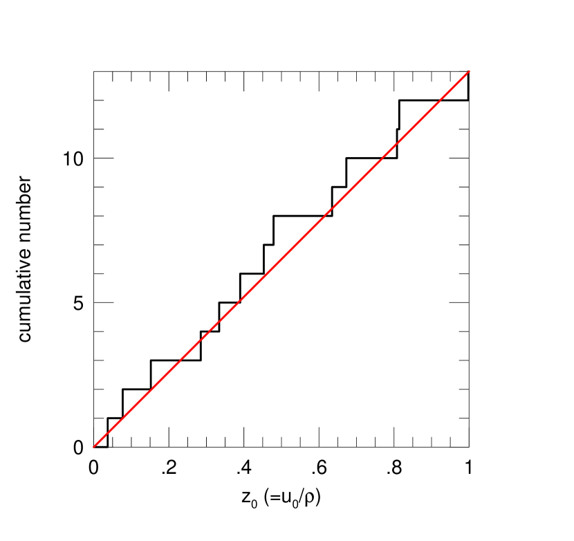
Figure 3: The cumulative distribution of $z_{0}\equiv u_{0}/\rho$ is quite consistent with a straight line, which would be the expected behavior for a sample without selection biases, In principle, it could be more difficult to detect finite-source effects for $z_{0}\simeq 1$ than lower values because the duration of these effects is shorter. However, this effect, if present, does not have a noticeable impact.

Figure 3 shows the cumulative distribution of $z_{0}\equiv u_{0}/\rho$. Under the assumption that there is no selection bias over the range $0\leq z_{0}\leq 1$, this should be a straight line. One may expect that it is more difficult to detect finite-source effects for $z_{0}\sim 1$, which would result in a deficit at these values, causing the cumulative distribution to flatten. This is because $z_{0}\sim 1$ events would seem to suffer deviations from a standard Paczyński (1986) curve for a shorter time, which would both increase the chance that these effects will be entirely missed due to gaps in the data, and reduce the statistical significance of detections to the extent that the data do capture this region. Contrary to this naive expectation, the cumulative distribution seen in Figure 3 is consistent with being uniform over $0<z<1$.

The cause of this robustness may be that finite-source deviations are actually relatively pronounced for $z\equiv u/\rho\gtrsim 1$. In the high magnification limit (which generally applies to most of the events in this sample), one finds using the hexadecapole approximation (Pejcha & Heyrovský, 2009; Gould, 2008) that the fractional change in magnification tends toward

$${\delta A\over A}\rightarrow{1-(1/5)\Gamma\over 8z^{2}}+{1-(11/35)\Gamma\over(64/3)z^{4}};\qquad(z>1),$$ (15)

where $\Gamma$ is the limb-darkening coefficient (see Section 4). Equation (15) actually works quite well almost to $z\rightarrow 1$ (Figure 3 from Chung et al. 2017). Hence, it shows that, e.g., at $z=\sqrt{2}$, the deviation is about $\delta A/A\sim 6.6\%$. Thus, for $z_{0}=1$, the deviations induced by finite-source effects remain at of order this level for $\sim 2t_{*}$. Giant-star events have two advantages in this regard. First, of course, $2t_{*}$ is longer for these events, typically 5 hours or more. However, there is also a second, more subtle effect. In events for which the lens does not actually transit the source, $\rho$ is highly degenerate with $u_{0}$, and for most high-magnification events, $u_{0}$ is degenerate with $t_{\rm E}$ and other parameters. Disentangling these degeneracies requires high quality data near baseline, i.e., $A\sim$ few. However, if the source is very faint, then the photometric errors near baseline are large compared to $(A-1)f_{s}$. But for giant sources, these fractional errors are much smaller unless the giant happens to be highly extincted. In brief, Figure 3 suggests that there is no strong bias against detection of finite-source effects at $z_{0}\sim 1$, and theoretical considerations tend to support this suggestion.

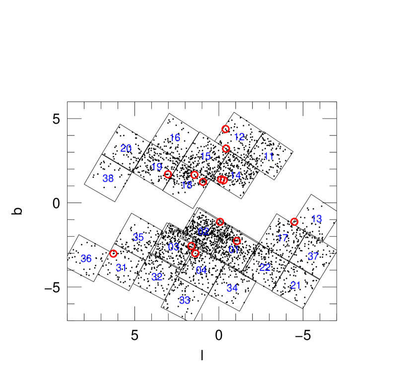
Figure 4: The distribution of 2019 KMT FSPL events (red) in Galactic coordinates compared to corresponding distribution of EventFinder events (black). The FSPL events may appear to “avoid” areas of high event concentration. However, while Figure 5 confirms this impression, it also shows that this feature is not statistically significant. The black squares outline the KMT fields, which are labeled with blue field numbers. Note that to avoid clutter, fields BLG41, BLG42, and BLG43 are shown, but not labeled. As shown, they lie toward slightly higher $b$ and lower $l$ compared to the corresponding fields BLG01, BLG02, and BLG03.

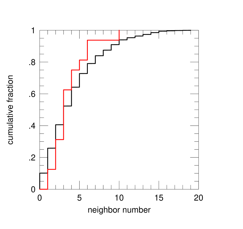
Figure 5: Cumulative distributions of 2019 FSPL events (red) compared to 2019 EventFinder events (black), ranked by number of EventFinder neighbors within $10^{\prime}$ (roughly the size of the red circles in Figure 4). While there is a higher fraction of higher-neighbor-number 2019 EventFinder events (in accord with the visual impression from Figure 4), this is not statistically significant.

Figure 4 shows the distribution of 2019 FSPL events in Galactic coordinates compared to 2019 EventFinder events. By eye, the FSPL events appear perhaps to avoid high-concentration areas of the EventFinder distribution. Figure 5 confirms that a larger fraction of EventFinder events have large numbers of near neighbors, but at the same time shows that this effect is not statistically significant.

Figure 4 also shows that there are more FSPL events in the northern bulge (7) than the southern bulge (6), despite the fact that only about 25% of KMT observations are toward the northern bulge. This is somewhat surprising but is also not statistically significant. First, we expect that detection of finite-source effects in giant-star events should be substantially less frequent in fields with nominal cadences $\Gamma\geq 1\,{\rm hr}^{-1}$ than those with $\Gamma\leq 0.4\,{\rm hr}^{-1}$, because the former are well sampled over the peak while the latter are relatively poorly sampled, given that typical giant-star $t_{*}\sim 7\,$hr. And indeed, there are only three of 13 events in the latter category (in fields BLG12, BLG13, and BLG31). All of the remaining 10 lie in the eight $\Gamma\geq 1\,{\rm hr}^{-1}$ fields that are grouped closest to the Galactic center, i.e., BLG01/41, BLG02/42, BLG03/43 and BLG04 in the south and BLG14, BLG15, BLG18, and BLG19 in the north. There are four events in the first group and six in the second, which is not significantly different. Thus there is no evidence for unexplained structure in the on-sky distribution of FSPL events.

Tables 2 and 4 show two different estimates of the dereddened source magnitude $I_{s,0}$. The first, $I_{s,0,\rm web}=I_{s,\rm web}-A_{I,\rm gonzalez}$ is derived from the pipeline-PSPL-fit source flux and the cataloged extinction estimate derived from Gonzalez et al. (2012). The second, from the CMD analysis, $I_{s,0,\rm cmd}=(I_{s}-I_{\rm cl})_{\rm dophot}+I_{\rm cl,0,nataf}$, is derived by adding the offset of the source relative to the clump in a DoPhot-based CMD to the dereddened magnitude of the clump from Table 1 of Nataf et al. (2013). Comparison shows that $I_{s,0,\rm web}$ is systematically fainter than $I_{s,0,\rm cmd}$, and that the scatter in these offsets is significantly larger than the absolute error in the $I_{s,0,\rm cmd}$ estimate, which is typically $\sigma(I_{s,0,\rm cmd})\lesssim 0.07\,$mag. That is, the statistical properties of the $I_{s,0}$ estimates used for event selection are significantly different than the true values. In order to understand the potential impact of this difference, it is first necessary to identify its origin.

With this aim, we define

$$X\equiv I_{s,0,\rm cmd}-I_{s,0,\rm web};\qquad Z\equiv I_{s,\rm best-fit-pys}-I_{s,\rm pipeline-pys}\qquad Y\equiv X-Z.$$ (16)

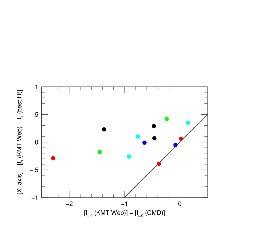
Figure 6: The abscissa “X-axis” shows the difference between the estimates of the dereddened source magnitude $I_{s,0}$ from the candidate selection process (KMT Web) and from the final (CMD) analysis. The ordinate shows the component of this difference that is due to everything except the difference between the pipeline-PSPL modeling of the event (without finite-source effects) and the human-supervised modeling with finite-source effects. The X-axis distribution displays large scatter and is strongly asymmetric. The Y-axis distribution has much smaller scatter and is symmetric about zero. This shows that essentially all of the systematic offset and most of the scatter is due to the pipeline-PSPL-modeling error, $Z=X-Y$. The values of $Z$ can be judged for individual points by noting their horizontal distance to the black diagonal line.

That is, $X$ is the difference in $I_{s,0}$ estimates, $Z$ is the portion of this difference that is due to a wrong pipeline-PSPL model, and $Y$ is the portion that is due to everything else. We will examine this “everything else” in detail below. But first we note that Figure 6, shows that “everything else” has essentially zero mean offset $\langle Y\rangle=0.03\pm 0.07$ and relatively small scatter, $\sigma(Y)=0.25$. This means that most of the scatter and all of the systematic offset of $X$ in Figure 6 is due to incorrect pipeline-PSPL modeling of the light curve. We will show that most of the scatter from “everything else” is due to the extinction estimate and the approximate calibration of KMT online photometry, both of which impact $I_{s,0,\rm web};$ rather than $I_{s,0,\rm cmd}$.

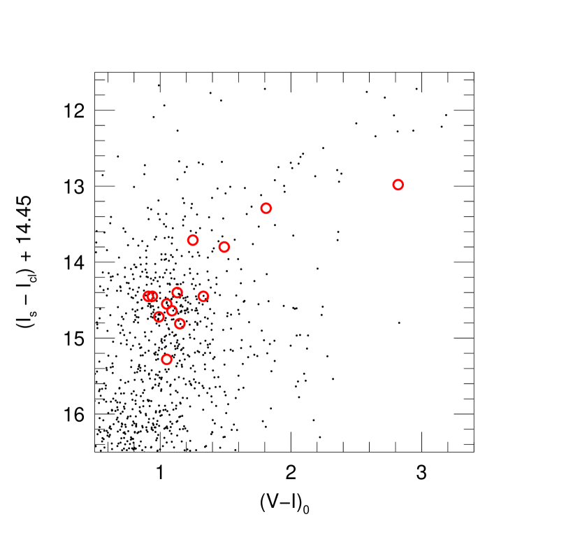
Figure 7: Location of each of the 13 FSPL events relative to the clump projected onto the dereddened CMD of KMT-2019-BLG-2555. As expected, the FSPL events generally trace the giant branch and red clump, but weighted toward brighter (so bigger, i.e., higher cross section) stars.

Therefore, the main consequence of the broad and asymmetric distribution of $X$ is that it affects selection. In particular, it removes of order a third of all candidates $16>I_{s,0,\rm true}>15$, as well as a few that are brighter, via Criterion (1). The unwanted rejection of potential candidates will, of course, adversely affect the size of the sample, but it will not in itself affect its statistical character. Each giant, regardless of how it is selected, should be equally sensitive to isolated lenses, regardless of their mass. The exception would be if the pipeline-PSPL modeling errors were more severe for low-mass events, so that more were artificially driven over the selection boundary by this effect. We see no evidence of this in our very small sample of two FFP candidates. But even if there were such an effect, its overall impact would be small because the affected region of the CMD $16>I_{s,0,\rm true}>15$ generates relatively few FSPL events, as we discuss in relation to Figure 7, below. And, as just mentioned, only about 1/3 of these are inadvertently eliminated.

We now turn to a more detailed investigation of the various independent terms grouped under $Y$, i.e., “everything else”. Rearranging terms in the equation $Y=X-Z$, we obtain

$$Y=[I_{s,\rm machine-pys}-I_{s,0,\rm web}]-[I_{s,\rm best-fit-pys}-I_{s,0,\rm cmd}].$$ (17)

Then, after several substitutions, this can be evaluated as,

$$Y=[A_{I,\rm gonzalez}-A_{I,\rm true}]-[{\rm Zpt}_{\rm pysis}-{\rm Zpt}_{\rm true}]+\delta_{\rm centroid}+[I_{\rm cl,0,nataf}-I_{\rm cl,0,true}]+\delta_{\rm pys-dop}.$$ (18)

These five terms are the error in $A_{I,\rm gonzalez}$ relative to the true value, the error in the adopted KMT pySIS zero point ($I=28$) relative to the true value, the error in fitting the clump centroid in the CMD, the error in that $I_{\rm cl,0}$ relative to the true value, and the offset between DoPhot and pySIS source-flux fit values relative to the true value (established by, e.g., field star comparison). The last is typically $<0.01$ mag and can be ignored. Apart from some unknown systematic offset, the penultimate term is also small because the intrinsic variation over the bar is smooth and the values in Nataf et al. (2013) Table 1 are established by averaging many measurements. The third term varies depending on the density of the clump but is typically 0.05 mag. The second term has two principal components: (1) the source counts for a star of fixed magnitude vary smoothly over the KMT field, with an effective dispersion of 0.05 mag, due to the optics, and (2) the transparency of the images chosen for the template of a given event can vary. We estimate the total dispersion of this term as 0.07 mag. Before examining the first term in detail, we note that given the total observed dispersion, $\sigma(Y)=0.25\,$mag, and our estimates of the other four terms, this leaves a dispersion of 0.23 mag for the first term. Several effects contribute. The first is the measurement error in the underlying Gonzalez et al. (2012) catalog, which includes errors in estimating the mean $A_{K}$ over the ($2^{\prime}\times 2^{\prime}$) grid point that is cataloged in the KMT database. The second is the difference between this true mean value and the actual value at the location of the event due both to smooth variation of $A_{K}$ and patchy extinction. The third is the difference between $A_{I}$ and our adopted universal estimate of this as $A_{I}=7A_{K}$. These effects can very plausibly account for the $0.2\,$mag “observed dispersion” that was estimated above. In principle, each of the first, second, and fourth terms could contain a systematic offset. However, if such systematic offsets are present, they happily cancel to within $\sim 0.06\,$mag.

The points in Figure 6 are color-coded according to $z_{0}\equiv u_{0}/\rho$. One may generally expect that the pipeline-PSPL fitting program will be “confused” by strong finite source effects ($z\lesssim 0.5$) because it does not contain $\rho$ as a fitting parameter. Indeed the three most severe outliers at the left all lie in this regime: KMT-2019-BLG-2555 ($z=0.334$), OGLE-2019-BLG-0953 ($z=0.479$), and KMT-2019-BLG-1143 ($z=0.077$). However, there are many other events with similar $z_{0}$ that suffer much smaller (or essentially no) pipeline-PSPL modeling problems. With one exception, we are not able to trace additional factors that distinguish the outliers from the others.

The exception is KMT-2019-BLG-2555. EventFinder assigned a catalog star to this event that was 4 mag fainter than the nearest catalog star (and actual source) of the event, which confused the pipeline-PSPL fit.

Figure 7 shows the positions of all the FSPL source stars relative to the clump centroid compared to the dereddened CMD of KMT-2019-BLG-2555. This event was chosen for the comparison due to its relatively densely populated CMD, although it does suffer relatively high extinction, $A_{I}=3.71$. Of course, this dereddening applies only to stars that lie behind the full column of dust seen toward the clump, but these account for the overwhelming majority of the field stars that lie in the part of the CMD that is displayed. Figure 7 shows that 12 of the 13 FSPL sources closely follow the track of red giants and clump giant stars from the CMD. Eight of these 12 are tightly grouped in the clump, which displays a strong overdensity in the field star distribution. One lies on the lower giant branch, below the clump: KMT-2019-BLG-0313. This event is projected close to the edge of a small dark cloud, so its position on the CMD was estimated using a special procedure. See Section 6.4.3. And three of the 12 lie on the upper giant branch. This distribution is qualitatively consistent with expectations. The clump stars are somewhat more numerous than the lower giant branch stars, and they are further favored both by their higher cross section and the fact that (based on the analysis of Figure 6) we expect the selection process to eliminate about a third of the FSPL events with $16>I_{s,0,\rm true}>15$. Similarly, the upper giant branch is substantially more thinly populated than the clump but is favored by higher cross section. There is also one “outlier”: KMT-2019-BLG-1143 at the extreme right. It lies about 0.75 mag below the roughly horizontal track of upper giant branch field stars. This could be explained either by the source being exceptionally metal rich or by it being $\sim 3\,{\rm kpc}$ behind the mean distance to the Galactic bar, either in the far disk or in the distant part of the bar itself. We further remark on this event in the notes on individual events, Section 6.4.5.

6.3.3 Distribution of $\theta_{\rm E}$

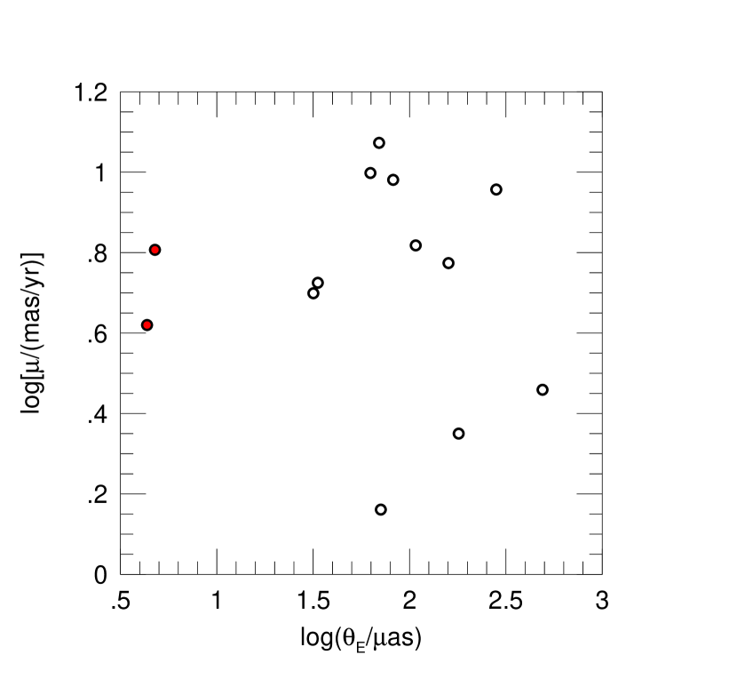
Figure 8: Plot of lens-source relative proper motion $\mu$ versus Einstein radius $\theta_{\rm E}$ for 13 FSPL giant source events from 2019. The median proper motion is $\mu_{\rm med}=5.9\,{\rm mas}\,{\rm yr}^{-1}$, which is typical of microlensing events with measured $\mu$. The two FFP candidates (red) have proper motions straddling the median, i.e., 4.2 and 6.4 ${\rm mas}\,{\rm yr}^{-1}$. The two FFP candidates lie well separated from the rest of the giant-star FSPL event in $\theta_{\rm E}$, which are otherwise evenly distributed in $\log\theta_{\rm E}$.

Figure 8 is a scatter plot of Einstein radius $\theta_{\rm E}$ versus lens-source relative proper motion $\mu$. The median proper motion is $\mu_{\rm med}=5.9\,{\rm mas}\,{\rm yr}^{-1}$, which is typical of microlensing events with measured $\mu$. Leaving aside the two events at the left edge of the distribution, the remaining 11 events have Einstein radii in the range $31\lesssim\theta_{\rm E}/\mu{\rm as}\lesssim 490$. That is, if all had the same $\pi_{\rm rel}$, then these lenses would span a factor $(490/31)^{2}=250$ in mass. For example, for $\pi_{\rm rel}=16\,\mu{\rm as}$, this mass range would be: $7.7\,M_{\rm jup}$ to $1.8\,M_{\odot}$. Of course, not all the lenses have the same $\pi_{\rm rel}$, but this simple calculation suggests that these FSPL events span a wide range of stellar and brown-dwarf masses. The two low-$\theta_{\rm E}$ events are FFP candidates.

6.4 Notes on Individual Events

6.4.1 OGLE-2019-BLG-1182

There are Spitzer data for this event, so it may ultimately yield an isolated-object mass measurement. However, the Spitzer data begin 3.53 days after $t_{0,\oplus}$, i.e., at $u_{\oplus}=1.13$ for this short $t_{\rm E}=3.13\,$day event. Hence, it is possible that the Spitzer parallax will only yield a relatively large circular-arc constraint in the ${\mbox{\boldmath$\pi$}}_{\rm E}$ plane (Gould, 2019).

6.4.2 KMT-2019-BLG-2800

There are no magnified $V$-band points for this short ($t_{\rm E}=2.14\,$day) event. However, the fit to DoPhot (Schechter et al., 1993) reductions shows that it is consistent with zero blending, so that the color can be estimated from the baseline object. We identify the baseline object on a $[Z-K,K]$ VVV (Minniti et al., 2017) CMD, from which we determine that it lies $\Delta(Z-K)=0.18$ mag redward of clump. Using an $(IZK)$ color-color diagram, we determine that this corresponds to $\Delta(I-K)=0.23$, and then using Bessell & Brett (1988), that this implies $\Delta(V-I)=0.27$. The resulting $\theta_{*}=8.1\,\mu{\rm as}$ leads to a relatively high lens-source relative proper motion, $\mu_{\rm rel}=11.8\,{\rm mas}\,{\rm yr}^{-1}$. However, this is less surprising after considering that the Gaia baseline-object proper motion is ${\mbox{\boldmath$\mu$}}_{\rm base}(N,E)=(-10.28,-4.72)\pm(0.32,0.39)\,{\rm mas}\,{\rm yr}^{-1}$. Given the low/zero blending, this measurement can be taken as a proxy for ${\mbox{\boldmath$\mu$}}_{s}$.

6.4.3 KMT-2019-BLG-0313

In the finding chart, this event is seen to lie near the edge of a small dark cloud, perhaps one of a string of such clouds that extends south-west to north-east, diagonally through the field. The cloud is far too small to form a CMD of stars of similar extinction, which is the normal basis of the Yoo et al. (2004) technique. Instead, we form such a CMD from the larger field and then project the source along the reddening vector, using a slope $R_{VI}=dI/d(V-I)=1.37$ until it hits the lower giant branch at $[(V-I),M_{I}]=(1.05,0.71)$.

6.4.4 KMT-2019-BLG-2528

This event is almost entirely contained in “pre-season” data taken at the end of the night, only from KMTC and only in $I$-band. This observing program was motivated to constrain the parallax measurement of KMT-2018-BLG-1292 (Ryu et al., 2019a), but was carried out in all western KMTNet fields. Hence, the source color cannot be measured from the light curve.

Unfortunately, the fit to DoPhot (Schechter et al., 1993) reductions shows that the source is blended, so we cannot simply derive the color from that of the baseline object. However, it is still the case that $\eta=f_{b}/f_{\rm base}=0.166$ is relatively small. We therefore begin with a modified version of this approach (see Section 6.4.2).

First, we find that the baseline object lies $\Delta(Z-K)=0.49$ redward of the clump. If we assume that the blend has the same color as the baseline object (which is extremely red) then we obtain from the $IZK$ color-color diagram that $\Delta(I-K)=0.62$. Then, following the same procedures as above, we derive $(V-I)_{\rm base,0}=1.69$, and so $(V-I)_{s,0}=1.69$.

However, because the blend is 1.75 mag fainter in $I$ than the source, hence $I_{0}\sim 14.88$, it most likely is a clump star or a first ascent giant just below the clump, and hence would have $(V-I)_{0,b}\sim 1.04$ and thus $\Delta(I-K)_{0,b}=-0.03$ relative to the clump. Then, instead of the blend accounting for 16.6% of the $K$ band light of the baseline object, it would account for only 9.9%. Thus, the source would be redder yet by $\delta(I-K)=0.08$ mag, implying $(V-I)_{s,0}=1.81$. Finally, conceivably, the blended light could be due to an extreme foreground object (e.g., the lens) in which case it would account for a tiny fraction of the $K$-band flux from the baseline object, and so $(V-I)_{s,0}\sim 1.9$. We finally adopt $(V-I)_{s,0}=1.81$, recognizing that there is some additional uncertainty in the color for this event. However, this added uncertainty has no material impact on the scientific conclusions in the current context.

6.4.5 KMT-2019-BLG-1143

This event has a complex discovery history and also posed some challenges in measuring the source color. The event designation KMT-2019-BLG-1143 derives from an alert posted to the KMT web page on 6 June (HJD${}^{\prime}=8640.66$) as “probable” microlensing, when the event was at magnification $A=14.6$, corresponding to an $I=14.4$ “difference star”. This is surprisingly late. Moreover, the subsequent DIA light curve used to classify alerts did not seem to confirm the microlensing interpretation, and it was reclassified as “not-ulens”. Then the same event was apparently “rediscovered” by EventFinder, with the DIA light curve tracing a very well defined and obvious microlensing event.

This puzzling discrepancy was resolved as follows. The EventFinder catalog star lies $3.5^{\prime\prime}$ roughly north of the AlertFinder catalog star. The AlertFinder program actually triggered on the former on 26 March, i.e., 72 days earlier, when the $(A-1)=0.22$ magnification produced a difference star of $I=18.9$. The candidate was then “misclassified” as a variable, and was thus not shown to the operator again as it further evolved. Then, as the event neared peak, it became so bright that the excess flux inside the more southerly catalog-star aperture rose sufficiently to trigger a human review. Finally, after the “rediscovery”, the program that cross matches AlertFinder and EventFinder discoveries identified them as the same event. Note that even if the KMT-2019-BLG-1143 had not been “rediscovered” by EventFinder, it would have been recognized as having the wrong coordinate centroid, which would have been corrected, in the end-of-year re-reductions. Unfortunately, in 2019 there was not sufficient computing power to properly re-centroid already discovered events contemporaneously with other real-time tasks. Otherwise, the event would have almost certainly been chosen as a Spitzer target.

The DoPhot fit shows that the source is blended with another much-bluer star that is $\Delta I=1.36\pm 0.07$ mag fainter. The blended star is well localized to lie in the clump, but the source $V$-band flux is not reliably measured. We therefore adopt a similar approach as for KMT-2019-BLG-2528 (Section 6.4.4), with two adjustments. First, we assume that the blend is a clump giant rather than considering a range of possibilities. Second, we adopt the 2MASS measurement $K=10.375$ in place of the VVV measurement $K=10.963$ because the latter is saturated. We then find that the source lies $\Delta(Z-K)=1.07$ mag redward of clump, which we transform to to $\Delta(I-K)=1.40$, and finally $\Delta(V-I)=1.76$. Because the source is an M giant, we use the M-giant color/surface-brightness relation of Groenewegen (2004) to evaluate $\theta_{*}$.

We note that KMT-2019-BLG-1143, which has the largest Einstein radius of the sample, $\theta_{\rm E}=489\,\mu{\rm as}$, also has a well-measured annual microlensing parallax, ${\mbox{\boldmath$\pi$}}_{\rm E}(N,E)=(0.146,0.278)$. Together these yield a lens mass $M=\theta_{\rm E}/\kappa\pi_{\rm E}=0.19\,M_{\odot}$ and relative parallax $\pi_{\rm rel}=0.154\,{\rm mas}$. Assuming that the source is in the bulge at $\pi_{s}=0.12\,{\rm mas}$, the lens distance is then $D_{L}=3.7\,{\rm kpc}.$

7 Discussion

7.1 Fourth FSPL FFP Candidate with $\theta_{\rm E}<10\,\mu{\rm as}$

KMT-2019-BLG-2073 is the fourth FFP candidate with measured $\theta_{\rm E}<10\,\mu{\rm as}$. The previous three had 3-4 year intervals between them: OGLE-2012-BLG-1323 (Mróz et al., 2019), OGLE-2016-BLG-1540 (Mróz et al., 2018), and OGLE-2019-BLG-0551 (Mróz et al., 2020). The discovery of KMT-2019-BLG-2073 in the same year as OGLE-2019-BLG-0551 (Mróz et al., 2020) may be just due to chance, but it could also reflect improved sensitivity of the KMT selection procedures to short FSPL events (e.g., searches for events with $t_{\rm eff}<1\,$day). KMT-2019-BLG-2073 was found independently by the AlertFinder in real time, and by the EventFinder in post-season analysis. The AlertFinder was in full operation for the first time in 2019. (In 2018, it essentially operated only in the northern bulge and only for about half the season). The EventFinder found it as a $t_{\rm eff}=0.42\,$day event. In 2016, the search was conducted only for $t_{\rm eff}\geq 1\,$day, and this remained so for 60% of sources in 2017. Hence, it is possible that FFP candidate events remain undiscovered in the database of KMT light curves.

7.2 Future Adaptive Optics Search for Host

A key open question for KMT-2019-BLG-2073 is whether or not the lens is indeed a free-floating planet rather than a planet on a wide orbit. In Section 5, we discussed the limits on a possible host star that can be inferred from the microlensing light curve alone. A more powerful test is to image the system directly to search for light from a host star. Due to the brightness of the source star, this is only really feasible by waiting for the lens and source to separate, so that light from the lens can be resolved.

Because the source is a bright giant $(J,H,K)_{s}=(15.28,14.16,13.72)$, a high contrast-ratio sensitivity is required to detect even the brightest putative host, i.e. a main-sequence star in the Galactic bulge. For example, for a Sun-like host in the bulge, the extincted apparent magnitudes would be, $(J,H,K)_{\rm sun-like}\simeq(19.7,18.7,18.3)$, and it would therefore have contrast ratios $\Delta(J,H,K)=(4.4,4.5,4.6)$ magnitudes.

As a point of comparison, Bowler et al. (2015) achieved contrast ratios of $\Delta K=5$ magnitudes for several of their targets at separations of $\Delta\theta=100\,$mas using a coronagraph on Keck. This comparison immediately raises three issues. First, at its measured lens-source relative proper motion $\mu_{\rm rel}=6.4\,{\rm mas}\,{\rm yr}^{-1}$, the system will not reach 100 mas separation until 2035. Second, at $K_{s}=13.7$, the source star is too faint for the Keck coronagraph. While conventional adaptive optics (AO) observations would be possible, their contrast performance is inferior to that of coronagraphs. Third, Bowler et al. (2015) found that the next significant improvement in contrast ratio came at $\Delta\theta=300\,$mas, where it increased to about $\Delta K=11$ magnitudes. See their Figure 3.

This comparison makes it clear that very little can be accomplished with current instruments for many decades. Long before this time, next-generation extremely large telescopes (ELTs) will come on line. Because planet imaging is a major driver for these projects, it is likely that they will mount coronagraphs. To be specific, we will consider that these are operational in 2032, i.e., when $\Delta\theta=83\,$mas. Scaling to the experience of Bowler et al. (2015), we estimate that the 39m European ELT (EELT) will achieve $\Delta K=11$ mag of contrast at $\Delta\theta=300/3.9=77\,$mas. That is, it could probe for putative bulge hosts down to $K=24.7$, i.e., $M_{K}=9.7$, which is below the bottom of the main sequence. While, as mentioned above, the source star is too faint for the Keck coronagraph, the magnitude limit for an EELT coronagraph should increase by $5\log(39/10)=3.0\,$mag, even without further improvements in instrument design. Thus it is plausible that an EELT coronagraph could probe for hosts down to the bottom of the main sequence.

We note that several other FFP candidates have favorable characteristics for EELT observation, including OGLE-2012-BLG-1323, KMT-2017-BLG-2820, OGLE-2016-BLG-1928, and OGLE-2016-BLG-1540, which will have separations of $\Delta\theta=112\,$mas, 128 mas, 138 mas, and 168 mas, respectively.

7.3 Future FFP Statistical Studies

In Section 6, we have presented a detailed outline of a statistical approach to measuring the relative frequency of FFP’s compared to stars and brown dwarfs. Our approach has two main features. First, it uses the $\theta_{\rm E}$ distribution, which is a more robust measure of lens mass than the $t_{\rm E}$ distribution. Second, we focus on events with giant sources, which are more likely to yield the finite source effects needed to measure $\theta_{\rm E}$ and have a number of other practical advantages (described in Section 6).

We apply this method to the 2019 season as a case study to identify and explore any unexpected challenges in this approach, we derived a sample of 43 giant-source events from the KMT event database, which was based on the union of events found by the AlertFinder and the EventFinder, together with a supplemental search using a version EventFinder that was tuned to giant source-star events with finite-source effects. We found that 13 were FSPL events, implying that they yielded measurements of $\rho$ and so $\theta_{*}$, $\theta_{\rm E}$, and $\mu$. We found a factor six gap in $\theta_{\rm E}$ between the two FFP candidates and the 11 other events. The cumulative distribution of the latter (Figure 9) is consistent with being linear in $\log\theta_{\rm E}$. That is, $dN/d\log\theta_{\rm E}\sim\,$const.

We emphasized at the outset (and we repeat here) that no scientific conclusions about FFPs can be drawn from this sample because it was motivated by an apparently “large number” (i.e., 2) of FFPs during the 2019 season, and so suffers from publication bias. In addition, to draw statistical conclusions about FFPs, one would have to study the selection function of low-$\theta_{\rm E}$ events in the underlying KMT database. As $\theta_{\rm E}$ is reduced, an FSPL light curve will become dominated by finite source effects rather than the Paczyński curve. Thus, the EventFinder and AlertFinder algorithms (built for PSPL curves) will eventually fail to identify the events as potential microlensing. And, even before that happens, the operator may fail to correctly classify the event as microlensing. Application of this approach to the full KMTNet sample and more detailed characterization of the selection function (e.g., through an injection-recovery test) will be the subject of future work, which is already underway (e.g., Ryu et al., 2021).

However, neither of these concerns weighs heavily for the sample of larger $\theta_{\rm E}$ events. Of these 11 events with FSPL effects, all were found by the EventFinder, and all but three (KMT-2019-BLG-2528, KMT-2019-BLG-2800, and KMT-2019-BLG-2555) were found by the AlertFinder. The first of these occurred in “pre-season” data, long before the AlertFinder started 2019 operations. The second peaked at HJD${}^{\prime}=8759$, i.e., Oct 2, and so 27 days after the AlertFinder had ceased operations. The third event peaked at HJD${}^{\prime}=8581$, i.e., Apr 7. This was 11 days after the AlertFinder began 2019 operations, so this event should have been found. Nevertheless, the failure rate for these events, which are typically both bright and relatively high-magnification is low. So the chance they would be missed by both search algorithms, or lie in the fraction of the season where they were only searched by EventFinder and missed, is also low. Furthermore all of the FSPL events were rediscovered by the special supplemental search that we carried out, except for the two that were excluded from this search because they had $t_{\rm eff}>5\,$ days (and so were expected to be easily detected in the regular searches). The first concern (publication bias) also does not apply to this subsample of 11: almost nothing was known about the subsample prior to undertaking this investigation.

We prefer to wait for a larger, multi-season sample of the higher-$\theta_{\rm E}$ events before undertaking a systematic investigation. However, here we would like to point out two robust features of the 2019 sample. First the fact that the $\theta_{\rm E}$ distribution is approximately uniform in $\log\theta_{\rm E}$ implies that lens mass distribution is consistent with being uniform in $\log M$. As we have emphasized, the event rate for FSPL events is directly proportional to their frequency. Hence, future statistical studies on a larger sample could probe this mass function.

Second, the paucity of lenses with $\theta_{\rm E}\lesssim 30\,\mu{\rm as}$ appears to be real. The first two events above this gap (KMT-2019-BLG-0703 and KMT-2019-BLG-2555) are bright, relatively high-magnification events that were easily selected for inspection by the EventFinder algorithm, and easily recognizable as microlensing in the completed-event visual inspection. Events like these are not likely to escape detection. Hence, this gap in the $\theta_{\rm E}$ distribution could reflect a dip in the mass function of isolated objects. A larger statistical sample will clarify this. Even better would be to directly measure masses for FFPs from a combination of $\theta_{\rm E}$ from finite source effects and $\pi_{\rm E}$ from satellite parallaxes (Gould et al., 2021). The experience gained now from FSPL searches is essential to planning such endeavors.

7.4 FFPs or Wide-Orbit Planets?

The main caveat with searches for microlensing FFPs is that, generally, one cannot be certain from the microlensing light curve alone that a planetary-mass lens is truly isolated. There are several ways to investigate whether or not the planetary-mass lens population is free-floating as opposed to having host stars at large separations (Ryu et al., 2021, also discuss this issue in detail). First, one can investigate the continuum of planets with increasing $s$ (e.g., Poleski et al., 2018, 2020) to see if this population is consistent with being an extension of the known population of bound planets. Second, the situation should be much clearer for the FFP candidate population probed by Roman (Johnson et al., 2020), because Roman will have FFP events with dwarf sources and will often have a sufficiently high-resolution to resolve out unrelated blends. Hence, Roman FFP candidates will either have detections of excess light due to a host star or much stronger limits on such light.

Third, the FFP candidates identified from ground-based FSPL events can be followed up using high-resolution imaging to search for host stars, as discussed in Section 7.2 for KMT-2019-BLG-2073. Because $\mu_{\rm rel}$ is directly measured for FSPL events, the separation between the lens and source can be predicted as a function of time. Hence, once enough time has passed, high-resolution imaging can be used to search for the flux from a host star. This ability to search for host stars is another major advantage of a $\theta_{\rm E}$-based study over one based on $t_{\rm E}$ (for which $\mu_{\rm rel}$ is unknown, so it can be difficult or impossible to definitively associate or exclude a given source with the event).

There are two caveats. First, the larger the separation of the lens and source, the more likely it is for an unrelated star to lie at the expected separation from the source. Second, if the planet is on a very wide (e.g., 1000 au) orbit, the host star will be sufficiently displaced from the lens to distort the measurement.

However, both of those caveats can be overcome simply by taking two epochs of high-resolution imaging. This will show that the magnitude of the proper motion matches that expected from the microlensing light curve. Furthermore, as discussed in Ryu et al. (2021) it can distinguish between planets in Kepler-like ($\sim 100$ au) and Oort-like ($\sim 1000$ au) orbits because while the magnitude of the host proper motion will be correct, the direction will be displaced from the direction of the source in proportion to the semi-major axis (see also Gould, 2016).

Table 1: Mean parameters for 1L1S models

Parameters	1L1S	1L1S ($f_{B}$=0)
$\chi^{2}/\rm{dof}$	4548.957/4549	4549.197/4549
$t_{0}$ $(\rm{HJD}^{\prime})$	8708.598 $\pm$ 0.005	8708.599 $\pm$ 0.004
$u_{0}$	0.241 $\pm$ 0.170	0.163 $\pm$ 0.103
$t_{\rm E}$ $(\rm{days})$	0.267 $\pm$ 0.026	0.272 $\pm$ 0.007
$\rho$	1.184 $\pm$ 0.142	1.138 $\pm$ 0.012
$f_{S}({\rm KMTC})$	0.947 $\pm$ 0.196	0.873 $\pm$ 0.001
$f_{B}({\rm KMTC})$	-0.073 $\pm$ 0.196	-
$t_{*}$ $(\rm{days})$	0.313 $\pm$ 0.011	0.310 $\pm$ 0.005
$\hat{S}$	0.673 $\pm$ 0.035	0.674 $\pm$ 0.014

Note. — $t_{*}\equiv\rho t_{\rm E}$ and $\hat{S}\equiv f_{S}/\rho^{2}$are derived quantities and are not fitted independently. All fluxes are on an 18th magnitude scale, e.g., $I_{S}=18-2.5\,\log(f_{S})$.

Table 2: Events selected for investigation

KMT Name	Name	$\mu_{\rm thresh}$	$\rho$ meas?	$u_{0}$	$t_{\rm E}$	$I_{s}$	$A_{I}$	$I_{s,0}$	$\Delta\chi^{2}$
KB191820	OB191182	24.23	Yes	0.024	3.38	16.17	1.44	14.73	11187
KB192800	KB192800	19.13	Yes	0.048	2.22	16.69	2.04	14.65	9392
KB191653	KB191653	16.50	Yes	0.012	9.22	17.41	2.52	14.89	3690
KB190313	KB190313	15.52	Yes	0.032	2.65	19.97	4.37	15.60	5305
KB190703	KB190703	15.28	Yes	0.035	3.32	17.78	2.83	14.95	12738
KB190853	OB190726	12.66	Yes	0.013	11.72	17.05	2.28	14.77	13201
KB192073	KB192073	11.17	Yes	0.324	0.50	18.68	3.77	14.91	2663
KB192528	KB192528	8.40	Yes	0.022	14.55	17.31	3.26	14.05	973
KB192555	KB192555	6.89	Yes	0.014	11.35	19.71	3.71	16.00	2450
KBS0111	KBS0111	6.10	No	0.088	2.96	21.52	6.33	15.19	1754
KB190352	KB190352	5.47	No	0.044	8.13	17.96	3.22	14.74	4276
KB192291	OB191408	5.43	No	0.109	2.03	17.86	2.06	15.80	1581
KB191335	KB191335	5.23	No	0.024	14.01	17.65	2.68	14.97	6777
KB191054	KB191054	4.89	No	0.017	16.28	19.78	4.24	15.54	4690
KB190061	OB190204	4.32	No	0.053	5.62	16.97	1.32	15.65	7140
KB192255	OB191415	3.54	No	0.166	6.35	15.00	1.66	13.34	17362
KB190519	OB190551	3.46	Yes	0.817	1.30	14.55	1.18	13.37	2180
KB192368	MB19006	3.05	No	0.087	12.68	15.19	1.63	13.56	23787
KB192542	OB191459	2.87	No	0.279	2.41	17.76	2.99	14.77	9479
KB191315	OB190953	2.86	Yes	0.005	78.29	19.36	3.41	15.95	2876
KB191143	KB191143	2.34	Yes	0.005	200.00	18.86	4.51	14.35	12675
KB191053	KB191053	2.29	No	0.493	5.03	16.84	4.41	12.43	14007
KB190289	KB190289	2.24	No	0.047	34.47	16.79	3.39	13.40	7111
KB190141	OB190171	1.82	No	0.025	36.56	18.22	3.13	15.09	14683
KB190863	KB190863	1.81	No	0.083	18.75	16.96	3.01	13.95	13343
KB192376	OB190382	1.80	No	0.388	2.94	16.22	1.58	14.64	2689
KB191039	OB190791	1.73	No	0.366	2.00	17.84	2.15	15.69	25760
KB190527	KB190527	1.65	Yes	0.033	26.73	18.66	3.28	15.38	4147
KB190007	OB190140	1.63	No	0.240	9.95	15.95	2.71	13.24	32049
KB190732	OB190698	1.62	No	0.275	3.99	16.27	1.32	14.95	20609
KB191030	KB191030	1.54	No	0.154	9.27	17.07	2.58	14.49	25535
KB192074	KB192074	1.49	No	0.067	18.14	18.45	3.54	14.91	11579
KB190125	OB190268	1.42	No	0.964	1.08	17.02	1.67	15.35	2568
KB192422	OB191462	1.30	No	0.181	9.10	18.87	4.33	14.54	23921
KB192297	KB192297	1.27	No	0.406	4.37	20.00	5.57	14.43	2810
KB192115	OB191307	1.25	No	0.045	23.81	16.98	1.41	15.57	4363
KB190424	KB190424	1.21	No	0.210	5.27	18.94	3.37	15.57	6724
KB191477	KB191477	1.12	No	0.289	3.84	20.46	4.73	15.73	689
KB190607	KB190607	1.11	No	0.057	30.01	16.63	1.83	14.80	11080
KB191677	KB191677	1.08	No	0.127	11.65	20.66	5.49	15.17	4728
KB190788	KB190788	1.06	No	0.209	7.90	19.03	4.04	14.99	8886
KB192263	OB191413	1.02	No	0.821	4.76	14.63	1.43	13.20	114120
KB192220	KB192220	1.01	No	0.783	3.85	19.99	6.22	13.77	642

Note. — Event names are abbreviations for, e.g., KMT-2019-BLG-1820, OGLE-2019-BLG-1182, and MOA-2019-BLG-006. In ”KBS0111”, ”S” indicates this event was identified in the ”Supplemental” search described in Section 6.2.2.

Table 3: Microlens Parameters for FSPL giant-star events

Name	KMT Name	$t_{0}$	$u_{0}$	$t_{\rm E}$	$\rho$	$f_{s,\rm KMTC}$
OB191182	KB191820	8695.82629	0.01998	3.129	0.07013	5.5886
	(errors)	0.00045	0.00088	0.014	0.00046	0.0384
KB192800	KB192800	8758.89773	0.04534	2.146	0.11617	3.3195
	(errors)	0.00364	0.01025	0.055	0.00352	0.1647
KB191653	KB191653	8684.67492	0.00232	5.975	0.06227	3.4576
	(errors)	0.00097	0.00000	0.044	0.00056	0.0323
KB190313	KB190313	8578.79642	0.06479	2.018	0.08018	0.2269
	(errors)	0.00083	0.00744	0.139	0.00699	0.0707
KB190703	KB190703	8613.40361	0.07759	2.312	0.17115	2.2435
	(errors)	0.00088	0.00333	0.028	0.00240	0.0446
OB190726	KB190853	8639.12940	-0.01649	11.315	0.02025	2.4698
	(errors)	0.00032	0.00009	0.032	0.00011	0.0084
KB192528	KB192528	8525.27942	0.07814	9.788	0.12306	3.4655
	(errors)	0.00544	0.00337	0.181	0.00239	0.0979
KB192555	KB192555	8581.05635	0.10038	2.302	0.30019	2.2663
	(errors)	0.00160	0.01421	0.059	0.00969	0.1087
OB190953	KB191315	8662.12889	-0.01594	29.253	0.03330	0.9185
	(errors)	0.00191	0.00076	1.035	0.00123	0.0361
KB191143	KB191143	8644.90325	0.00668	62.192	0.06143	1.9834
	(errors)	0.00145	0.00052	0.329	0.00035	0.0124
KB190527	KB190527	8620.78990	0.07092	17.955	0.07107	0.9385
	(errors)	0.00343	0.00178	0.234	0.00246	0.0170

Note. — Event names are abbreviations for, e.g., KMT-2019-BLG-1820. Fluxes are in units of $I=18$ system. For KB192073, see Table 1. For OB190551 (=KB190519), see Mróz et al. (2020).

Table 4: CMD and Derived Parameters for FSPL giant-star events

Name	KMT Name	RA	Dec	$(V-I)_{0}$	$I_{0}$	$\theta_{*}$	$\theta_{\rm E}$	$\mu_{\rm rel}$	$\mu_{\rm thresh}$	$z=u_{0}/\rho$
OB191182	KB191820	18:00:41.45	-29:15:42.80	1.15	14.75	5.86	82.19	9.58	24.23	0.285
KB192800	KB192800	18:11:24.09	-25:01:07.25	1.33	14.27	8.08	69.54	11.84	19.13	0.390
KB191653	KB191653	17:32:12.87	-27:35:16.91	1.13	14.42	6.58	107.60	6.58	16.50	0.037
KB190313	KB190313	17:42:38.85	-26:50:16.33	1.05	15.22	4.30	62.68	9.95	15.52	0.808
KB190703	KB190703	17:46:11.29	-25:28:43.72	0.91	14.35	5.42	31.69	5.00	15.28	0.453
OB190726	KB190853	17:51:43.04	-31:08:50.89	1.09	14.69	5.71	281.97	9.06	12.66	0.814
KB192073	KB192073	17:49:53.08	-29:35:17.30	0.94	14.45	5.43	4.77	6.41	11.17	0.152
KB192528	KB192528	17:39:03.05	-33:20:43.91	1.81	13.13	19.59	159.27	5.94	8.40	0.635
KB192555	KB192555	17:39:54.97	-28:19:46.74	1.25	13.71	10.04	33.44	5.31	6.89	0.334
OB190551	KB190519	17:59:28.75	-28:50:25.80	1.49	12.61	19.50	4.35	4.17	3.46	0.673
OB190953	KB191315	17:43:02.79	-27:29:12.26	1.05	14.50	5.99	179.88	2.24	2.86	0.479
KB191143	KB191143	17:39:43.02	-28:28:40.94	2.82	12.98	30.10	489.43	2.88	2.34	0.077
KB190527	KB190527	17:27:54.38	-26:55:30.22	0.99	14.74	5.05	71.03	1.45	1.65	0.998

Note. — Event names are abbreviations for, e.g., KMT-2019-BLG-1820, OGLE-2019-BLG-1182, and MOA-2019-BLG-006

Figure 9: Cumulative distribution of log Einstein radii $\log\theta_{\rm E}$ for 13 giant-star FSPL events from 2019. The cumulative distribution is consistent with linear for $\theta_{\rm E}\gtrsim 30\,\mu{\rm as}$, i.e., a flat differential distribution. Because $M=0.0069\,M_{\odot}(\theta_{\rm E}/30\,\mu{\rm as})^{2}/(\pi_{\rm rel}/16\,\mu{\rm as})$ this uniform-in-log distribution corresponds to a wide range of stellar and brown dwarf masses. The sudden plateau below $\theta_{\rm E}<30\,\mu{\rm as}$, may reflect a real absence of lower-mass objects. However, the apparent excess events (within this “desert”) at $\theta_{\rm E}\sim 5\,\mu{\rm as}$ cannot be used to make inferences about FFPs, due to publication bias.

References

- Agol (2003) Agol, E., 2003, ApJ, 594, 449
- Alard & Lupton (1998) Alard, C. & Lupton, R.H.,1998, ApJ, 503, 325
- Albrow et al. (2009) Albrow, M. D., Horne, K., Bramich, D. M., et al. 2009, MNRAS, 397, 2099
- Bennett et al. (2020) Bennett, D. P., Bhattacharya, A., Beaulieu, J. P., et al. 2020, AJ, 159, 68
- Bensby et al. (2013) Bensby, T. Yee, J.C., Feltzing, S. et al. 2013, A&A, 549A, 147
- Bessell & Brett (1988) Bessell, M.S., & Brett, J.M. 1988, PASP, 100, 1134
- Bowler et al. (2015) Bowler, B. P., Liu, M. C., Shkolnik, E. L., Tamura, M. 2015, ApJS, 216, 7
- Chung et al. (2017) Chung, S.-J., Zhu, W., Udalski, A., 2017, ApJ, 838, 154
- Dong et al. (2009) Dong, S., Bond, I.A., Gould, A., et al. 2009, ApJ, 695, 970
- Gonzalez et al. (2012) Gonzalez, O. A., Rejkuba, M., Zoccali, M., et al. 2012, A&A, 543, A13
- Gould (1996) Gould, A. 1996, ApJ, 470, 201
- Gould (2008) Gould, A. 2008, ApJ, 681, 1593
- Gould (2016) Gould, A. 2016, JKAS, 49, 123
- Gould (2019) Gould, A. 2019, JKAS, 52, 121
- Gould et al. (2021) Gould, A., Zang W., Mao, S., Dong, S. 2021, RAA, in press
- Gould & Yee (2012) Gould, A. & Yee, J.C. 2012, ApJ, 755, L17
- Groenewegen (2004) Groenewegen, M.A.T., 2004, MNRAS, 353, 903
- Han et al. (2020) Han, C., Lee, C.-U., et al. 2020, AJ, 159, 134
- Hirao et al. (2020) Hirao, Y., Bennett, D.P., Ryu, Y.-H., et al., 2020, in press
- Johnson et al. (2020) Johnson, S.A., Penny, M., Gaudi, B.S., et al. 2020, AJ, 160, 123
- Kervella et al. (2004) Kervella, P., Thévenin, F., Di Folco, E., & Ségransan, D. 2004, A&A, 426, 297
- Kim et al. (2016) Kim, S.-L., Lee, C.-U., Park, B.-G., et al. 2016, JKAS, 49, 37
- Kim et al. (2018a) Kim, D.-J., Kim, H.-W., Hwang, K.-H., et al., 2018a, AJ, 155, 76
- Kim et al. (2018b) Kim, D.-J., Hwang, K.-H., Shvartzvald, et al. 2018b, arXiv:1806.07545
- Maeder (1973) Maeder, A., 1973, A&A, 26, 215
- Minniti et al. (2017) Minniti, D., Lucas, P., VVV Team, 2017, yCAT 2348, 0
- Mróz et al. (2017) Mróz, P., Udalski, A., Skowron, J., et al. 2017, Nature, 548, 183
- Mróz et al. (2018) Mróz, P., Ryu, Y.-H., Skowron, J., et al. 2018, AJ, 155, 121
- Mróz et al. (2019) Mróz, P., Udalski, A., Bennett, D.P.., et al. 2019, A&A, 622, A201
- Mróz et al. (2020) Mróz, P., Poleski, R., Han, C., et al. 2020, AJ, 159, 262
- Nataf et al. (2013) Nataf, D.M., Gould, A., Fouqué, P. et al. 2013, ApJ, 769, 88
- Paczyński (1986) Paczyński, B. 1986, ApJ, 304, 1
- Pejcha & Heyrovský (2009) Pejcha, O., & Heyrovský, D. 2009, ApJ, 690, 1772
- Poleski et al. (2018) Poleski, R., Gaudi, B.S., Udalski, A. et al. 2018, AJ, 156, 104
- Poleski et al. (2020) Poleski, R., et al., 2020, in prep
- Riffeser et al. (2006) Riffeser, A., Fliri, J., Seitz, S., & Bender, R. 2006, ApJS, 163, 225
- Ryu et al. (2019a) Ryu, Y.-H., Navarro, M.G., Gould, A. et al. 2019, AJ, 159, 58
- Ryu et al. (2021) Ryu, Y.-H., Mróz, P., Gould, A. et al. 2021, AJ, 161, 126
- Schechter et al. (1993) Schechter, P.L., Mateo, M., & Saha, A. 1993, PASP, 105, 1342
- Schlafly et al. (2018) Schlafly, E.F., Green, G.M., Lang, D. et al. 2018, ApJS, 234, 39
- Sumi et al. (2011) Sumi, T., Kamiya, K., Bennett, D. P., et al. 2011, Nature, 473, 349
- Szymański et al. (2011) Szymański, M.K., Udalski, A., Soszyński, I., et al. 2011, Acta Astron., 61, 83
- Tomaney & Crotts (1996) Tomaney, A.B. & Crotts, A.P.S. 1996, AU, 112, 2872
- Yoo et al. (2004) Yoo, J., DePoy, D.L., Gal-Yam, A. et al. 2004, ApJ, 603, 139