MULTIVARIATE SIGNAL DENOISING BASED ON GENERIC MULTIVARIATE DETRENDED FLUCTUATION ANALYSIS

Abstract

We propose a novel multivariate signal denoising method that performs long-range correlation analysis of multiple modes in input data by considering inherent inter-channel dependencies of the data. That is achieved through a novel and generic multivariate extension of detrended fluctuation analysis (DFA) method - another contribution of this paper. Specifically, our proposed denoising method first obtains data driven multiscale signal representation using multivariate variational mode decomposition (MVMD) method. Then, the proposed generic multivariate DFA is used to reject the predominantly noisy modes based on their randomness scores. Finally, the denoised signal is reconstructed by summing the remaining modes albeit after the removal of the noise traces using the principal component analysis (PCA).

Index Terms—  Multivariate signals, Detrended fluctuation Analysis, Multivariate variational mode decomposition.

1 Introduction

Multi-sensor systems have found widespread use in many applications including medical diagnosis, health monitoring, weather forecasting etc. Within these systems, a network of synchronized sensors is used to record signals originating from physical system(s) resulting in interdependent multichannel observations. Those observations, denoted by $\boldsymbol{x}_{i}\in\mathcal{R}^{m}$, are modelled as a combination of the desired signal $\boldsymbol{s}_{i}\in\mathcal{R}^{m}$ and the unwanted noise $\boldsymbol{\psi}_{i}=\mathcal{R}^{m}$, as follows

$$\boldsymbol{x}_{i}=\boldsymbol{s}_{i}+\boldsymbol{\psi}_{i},\ \ \forall\ \ i=1,\ldots,N.$$ (1)

Estimation of true multivariate signal $\boldsymbol{s}_{i}$ from raw signal recordings $\boldsymbol{x}_{i}$ is a problem of considerable interest. To solve this problem, most of the existing algorithms are direct multichannel extensions of the popular multiscale approaches that have worked extremely well on univariate (single-channel) data. For instance, the sparsity of discrete wavelet transform (DWT) is exploited to reject noise via a multichannel expansion of the universal threshold [1]. Similarly, multiscale denoising approaches for multivariate data that are based on synchrosqueezed wavelet transform [2], multivariate empirical mode decomposition (MEMD) [3, 4] and translation invariant DWT aided by Mahalanobis distance measure [5], are extensions of [6, 7, 8, 9] respectively. Moreover, variational mode decomposition (VMD) algorithm [10] and its multivariate extension [11] have been employed for denoising [12, 13, 14]. In [12], detrended fluctuation analysis (DFA) [15] has been used to identify and reject the signal modes with predominant noise by estimating their long-range correlations.

In its original form, DFA only caters for single-channel time series data. While its multichannel extension exists [16], it processes each data channel in isolation thereby ignoring inter-channel correlations within multivariate data. To that end, we first develop a novel and generic multichannel extension of DFA, termed GMDFA in the sequel, that fully incorporates inter-channel correlations within data using Mahalanobis distance. Then, using that extension, we present a novel multichannel multiscale denoising method that first uses MVMD to decompose a multivariate data into multiple frequency modes; and then identifies (and rejects) the noisy modes using GMDFA. The efficacy of the proposed approach is demonstrated on a variety of real multichannel signals.

2 Detrended Fluctuation Analysis

The detrended fluctuation analysis (DFA) is widely used to estimate the extent of long-range correlations in a nonstationary time series. The main advantage of using DFA is that it circumvents the artefacts of nonstationarity (e.g., local trend, noise etc.,) which cause spurious scores in the otherwise used Hurst exponent method [15]. Specifically, DFA estimates a power law scaling exponent by observing natural variability of signal fluctuations around its local trend at different time scales. As a result, intrinsic fluctuations of a time series are extracted by detrending the slowly oscillating background that causes spurious scores [15] as described below:

Given a time series $x_{i},\ \forall\ i=1,...,N$; its normalized cumulative sum is obtained as follows: $\small{y_{i}=\frac{1}{N}\sum_{i=1}^{N}(x_{i}-\overline{x})}$, where $\overline{x}$ denotes the signal mean. The resulting profile $y_{i}$ is then divided into $N_{s}=N/s$ segments of equal length $s$ from both ends. Next, least squares polynomial fitting approach is employed on the resulting segments to estimate the local trend, denoted by $\tilde{y}_{i}$. Finally, a root mean squared (RMS) function $F(s)$ of detrended fluctuations $y_{i}-\tilde{y}_{i}$ is obtained as

$$\small{F(s)=\sqrt{\frac{1}{2N_{s}}\sum_{v=1}^{2N_{s}}\left(\frac{1}{s}\sum_{i=1}^{s}\left(y_{i}-\tilde{y}_{i}\right)^{2}\right)}.}$$ (2)

Note from (2) that $F(s)$ is the root mean of local (segment) variances that is expected to increase with increase in the time scale $s$. This increase in $F(s)$, when described using the power law relation of the time scale $s$ reflects on the long range correlations of a time series [17]. Specifically, the scale exponent $\alpha$ indicates long-range correlations if $\alpha>0.5$; while the cases of $\alpha=0.5$ and $\alpha<0.5$ suggest no-correlations and short-range correlations, respectively. Furthermore, $\alpha$ informs about the degree of smoothness of a time series, i.e., a higher value $\alpha$ indicates the presence of slow fluctuations while a lower $\alpha$ hints at rapid fluctuations [18]. The resulting insight gained through DFA renders it suitable in many signal processing related applications involving signal analysis [19] and denoising [12].

A multichannel DFA is presented in [16] using a straightforward multichannel generalization of (2) which is given by

$$\small{F_{m}^{{}^{\prime}}(s)=\sqrt{\frac{1}{2N_{s}}\sum_{v=1}^{2N_{s}}\Big{(}\frac{1}{s}\sum_{i=1}^{s}\sum_{n=1}^{m}\left(y_{i_{n}}-\tilde{y}_{i_{n}}\right)^{2}\Big{)}},}$$ (3)

where $y_{i_{n}}$ and $\tilde{y}_{i_{n}}$ respectively denote the profile and polynomial fit for the $n$th channel. Observe from (3) that the Euclidean norm of each $m$-variate error observation is used to formulate a multichannel fluctuation function $F_{m}^{{}^{\prime}}(s)$ in [16] which completely disregards the cross-channel correlations in the data and leads to spurious long range correlation scores.

3 Proposed Methodology

This section outlines our proposed multiscale multivariate signal denoising method. For this purpose, we first describe the proposed generic multichannel extension of DFA that underpins our denoising framework.

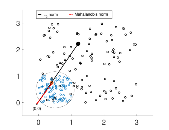
Fig. 1: Relocation of a set of points in 2D space (black circles) to another set (blue circles) through Mahalanobis distance norm. The black line shows the standard euclidean norm of a single point in 2D; the red line shows the corresponding Mahalanobis norm of the same point, which is more accurate since it considers cross-correlations and is robust to variance bias across the channels of multivariate data.

3.1 A Generic Multichannel Extension of DFA

To address the aforementioned weakness in the existing DFA in [14], we propose a novel multichannel extension of the DFA method that considers cross-correlations via Mahalanobis distance (MD) measure and may be seen as a generalization of [16]. The steps involved in the proposed Generic Multichannel DFA, termed GMDFA, are given below:

Given a multivariate time series $\boldsymbol{x}_{i}\ \forall\ i=1,...,N$, where $\boldsymbol{x}_{i}=[x_{i_{1}},\ldots,x_{i_{m}}]^{T}\in\mathcal{R}^{m}$ represents an $m$-variate observation at time index $i$, the cumulative sum $\boldsymbol{y}_{i}$ is computed via

$$\small{\boldsymbol{y}_{i}=\frac{1}{N}\sum_{i=1}^{N}(\boldsymbol{x}_{i}-\boldsymbol{\overline{x}}),}\vspace{-2mm}$$ (4)

where $\boldsymbol{\overline{x}}=\frac{1}{N}\sum_{i=1}^{N}\boldsymbol{x}_{i}$ denotes the multichannel mean.

Next, the signal $\boldsymbol{y}_{i}=y_{i_{n}}\}_{n=1}^{m}$ for all $i=1,\ldots,N$, is divided in $2N_{s}$ spatial segments by cutting it into $N_{s}=N/s$ segments of equal lengths starting from both ends of the series. Then, the local trend $\tilde{\boldsymbol{y}}_{i}=\tilde{y}_{i_{n}}\}_{n=1}^{m}$ is estimated based on the quadratic polynomial fit of each channel

$$\tilde{y}_{i_{n}}=a_{n}\cdot i^{2}+b_{n}\cdot i+c_{n},\ \ \ \ i=1,\cdots,s,$$ (5)

where $a_{n},b_{n},c_{n}$ denote the coefficients required for the least square fit $\tilde{y}_{i_{n}}\sim y_{i_{n}}$. Here, quadratic polynomial is used to estimate the slowly varying background trend. We next provide the mathematical definition of Mahalanobis norm which forms the basis of our proposed method.

Definition 1 (Mahalanobis norm)

Let $\Sigma$ denote a symmetric and positive definite covariance matrix of vector observations $\boldsymbol{z}_{i}\}_{i=1}^{N}$, we define the Mahalanobis norm $\|\boldsymbol{z}_{i}\|_{\Sigma}=\sqrt{\boldsymbol{z}_{i}^{T}\Sigma^{-1}\boldsymbol{z}_{i}}$ that satisfies the following properties of a norm on that vector space $\mathcal{Z}$, i.e.,

1. $\|\boldsymbol{z}\|_{\Sigma}>0\ \forall\ \boldsymbol{z}\neq\boldsymbol{0}$;

2. $\|\boldsymbol{z}\|_{\Sigma}=0$ iff $\boldsymbol{z}=\boldsymbol{0}$;

3. $\|a\boldsymbol{z}\|_{\Sigma}=|a|\cdot\|\boldsymbol{z}\|_{\Sigma}$ for a scalar $a$;

4. $\|\boldsymbol{z}_{1}+\boldsymbol{z}_{2}\|_{\Sigma}\leq\|\boldsymbol{z}_{1}\|_{\Sigma}+\|\boldsymbol{z}_{2}\|_{\Sigma}$.

where the vectors $\boldsymbol{z}$, $\boldsymbol{z}_{1}$ and $\boldsymbol{z}_{2}$ belong to the space $\mathcal{Z}$.

Remark 1

Mahalanobis norm $\|\boldsymbol{z}_{i}\|_{\Sigma}$ is a generalized multivariate norm because (a) it considers cross channel dependencies which are completely ignored within the $L_{2}$ norm; and (b) it performs variance normalization to remove variance bias across the channels (as depicted in Fig 1).

That can be observed from the following two cases of uncorrelated multivariate data where $\|\boldsymbol{z}_{i}\|_{\Sigma}$ reduces to a form of $\|\boldsymbol{z}_{i}\|_{2}$. Firstly, when $\tiny{\Sigma=I_{m\times m}}$ that denotes an identity matrix, $\|\boldsymbol{z}_{i}\|_{\Sigma}$ is given by

$$\small{\|\boldsymbol{z}_{i}\|_{\tiny{\Sigma=I_{m\times m}}}=\sqrt{\boldsymbol{z}_{i}^{T}I_{m\times m}^{-1}\boldsymbol{z}_{i}}=\sqrt{\boldsymbol{z}_{i}^{T}\boldsymbol{z}_{i}}=\|\boldsymbol{z}_{i}\|_{2}}.\vspace{-1mm}$$ (6)

Secondly, when $\Sigma=\boldsymbol{\sigma}^{T}I_{m\times m}$ is a diagonal matrix where the vector $\boldsymbol{\sigma}=[\sigma_{1},\sigma_{2},\ldots,\sigma_{m}]^{T}$ contains channel variances, $\|\boldsymbol{z}_{i}\|_{\Sigma}$ is given by

$$\small{\|\boldsymbol{z}_{i}\|_{\tiny{\Sigma=\boldsymbol{\sigma}^{T}I_{m\times m}}}=\sqrt{\left(\frac{z_{i_{1}}}{\sigma_{1}}\right)^{2}+\ldots+\left(\frac{z_{i_{m}}}{\sigma_{m}}\right)^{2}}=\|\overline{\boldsymbol{z}}_{i}\|_{2}},\vspace{-1mm}$$ (7)

where $\boldsymbol{z}_{i}=[z_{i_{1}},\ldots,z_{i_{m}}]^{T}$ and $\overline{\boldsymbol{z}}_{i}=[\frac{z_{i_{1}}}{\sigma_{1}},\ldots,\frac{z_{i_{m}}}{\sigma_{m}}]^{T}$.

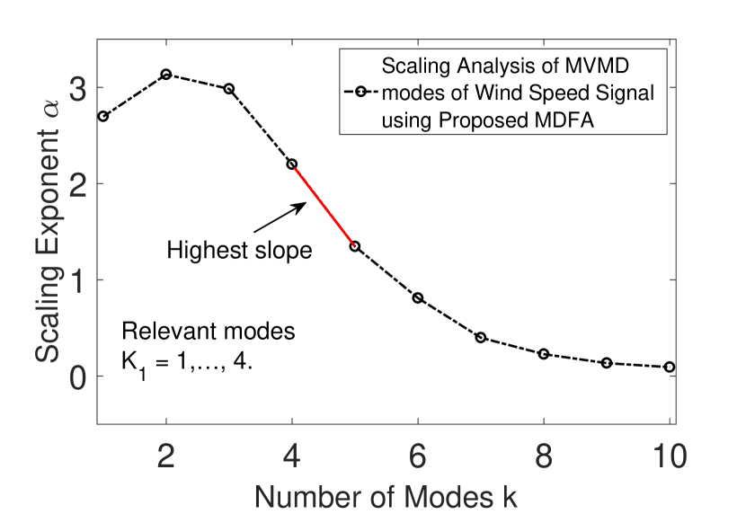
Fig. 2: Plot of scaling exponents $\alpha_{k}$, computed using proposed GMDFA, for MVMD modes of noisy Wind signal at $10$ dB.

Finally, in the case of correlated multivariate data, Mahalanobis norm essentially computes the $L_{2}$ norm by un-correlating the variance normalized vector observations as depicted in Fig. 1. For a special case of bivariate data, $\|\boldsymbol{z}_{i}\|_{\Sigma}$ can be rewritten as

$$\small{\|\boldsymbol{z}_{i}\|_{\Sigma}=\frac{1}{\sqrt{1-\rho^{2}}}\sqrt{\|\overline{\boldsymbol{z}}_{i}\|_{2}^{2}-\frac{2\rho z_{i_{1}}z_{i_{2}}}{\sigma_{1}\sigma_{2}}}},\vspace{-2mm}$$ (8)

where $\rho$ denotes correlation coefficient and $\Sigma=\tiny{\begin{pmatrix}\sigma_{1}^{2}&\rho\sigma_{1}\sigma_{2}\\ \rho\sigma_{1}\sigma_{2}&\sigma_{2}^{2}\end{pmatrix}}$.

Based on remark 1, we utilize the generic (Mahalanobis) norm $\|\boldsymbol{y}_{i}-\tilde{\boldsymbol{y}}_{i}\|_{\Sigma}$ to formulate a purely multivariate fluctuation function $F_{m}^{\Sigma}(s)$ within MDFA, that is,

$$\small{F_{m}^{\Sigma}(s)=\sqrt{\frac{1}{2sN_{s}}\sum_{v=1}^{2N_{s}}\sum_{i=vs+1}^{(v+1)s}\left(\boldsymbol{y}_{i}-\tilde{\boldsymbol{y}}_{i}\right)^{T}\Sigma^{-1}\left(\boldsymbol{y}_{i}-\tilde{\boldsymbol{y}}_{i}\right)}},$$ (9)

where covariance matrix $\Sigma$ characterizes the interchannel dependencies within the detrend (or fluctuations) $\boldsymbol{y}_{i}-\tilde{\boldsymbol{y}}_{i}$.

It is clear that (3) becomes a special case of (9) for identity covariance matrix, i.e., uncorrelated input multichannel data. For more interesting cases involving multichannel data that exhibit cross-channel correlations, (9) provides more informative fluctuation scores.

In order to perform multichannel scaling analysis in (9), $F_{m}^{\Sigma}(s)$ is computed for varying time scales where generally the range $s=4,\ldots,16$ is used [17]. Finally, a scaling exponent $\alpha$ is computed using power law representation of $F_{m}^{\Sigma}(s)$

$$\vspace{-2mm}F_{m}^{\Sigma}(s)=s^{\alpha}.$$ (10)

In practice, $\alpha$ is calculated based on the slope of the plot between $lnF_{m}^{\Sigma}(s)$ and $ln\ s$ because $log_{s}F_{m}^{\Sigma}(s)=\frac{lnF_{m}^{\Sigma}(s)}{ln\ s}$, where $ln$ denotes the natural logarithm operator.

3.2 Multiavriate Denoising Using MVMD and GMDFA

Here, we present a multivariate signal denoising method that applies the proposed GMDFA on the data-driven modes of noisy signal obtained from MVMD, as discussed below:

3.2.1 Multiscale decomposition using MVMD

Multivariate VMD [11] is a generic multichannel extension of the VMD algorithm that decomposes a multivariate signal $\boldsymbol{x}_{i}\in\mathcal{R}^{m}$ into $K$ number of predefined multivariate modulated oscillations $\boldsymbol{u}_{k,i}\in\mathcal{R}^{m}$ which are based on a common frequency component across all channels.

$$\small{\boldsymbol{x}_{i_{n}}=\sum_{k=1}^{K}\boldsymbol{u}_{k,i_{n}}}.$$ (11)

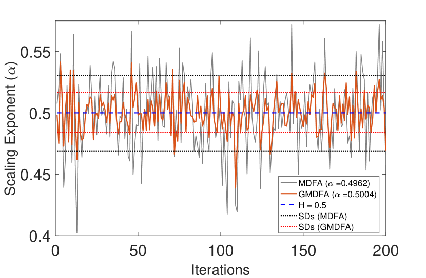
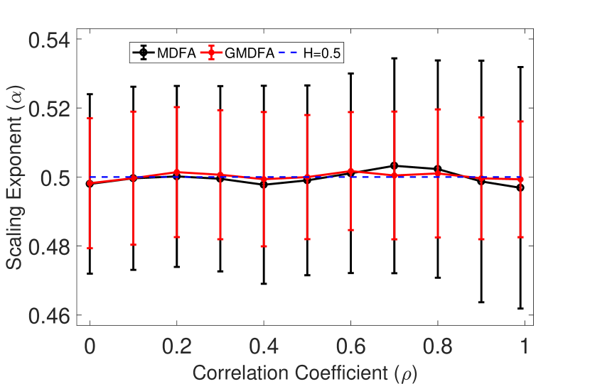
Fig. 3: Numerical simulations on bivariate white gaussian noise (wGn) for estimation of the Hurst exponent $H=0.5$ using MDFA [16] and GMDFA at varying degrees of cross-correlation.

Within our proposed denoising approach, firstly MVMD is used to decompose a noisy multivariate signal $\boldsymbol{x}_{i}$ into an ensemble of $K$ multichannel BLIMFs $\boldsymbol{u}_{k,i}$ which comprise of modulated multivariate oscillations of a common frequency component. Among those, initial BLIMFs contain low frequency (or smooth) oscillations whereas the latter BLIMFs mostly comprise of high frequency fluctuations. This representation can be mathematically written as

$$\small{\boldsymbol{x}_{i}=\sum_{k=1}^{K}\boldsymbol{u}_{k,i}=\sum_{k=1}^{K_{1}}\boldsymbol{u}_{k,i}+\sum_{k=K_{1}+1}^{K}\boldsymbol{u}_{k,i}},\ \forall\ i=1,\ldots,N,\vspace{-2mm}$$ (12)

where $\{\boldsymbol{u}_{k,i}\}_{k=1}^{K_{1}}$ denotes the set of initial BLIMFs containing majority of (true) signal and $\{\boldsymbol{u}_{k,i}\}_{k=K_{1}+1}^{K}$ denotes the BLIMFs with predominant noise. Next, MDFA is used to detect the predominant noise modes, i.e., $K_{1}$.

3.2.2 Rejection of predominantly noisy BLIMFs using MDFA

The proposed GMDFA is used to identify and discard predominantly noisy BLIMFs based on (a) their higher frequency content and (b) absence of long-range auto-correlations. In this regard, the comparative analysis of the scaling exponents $\alpha_{k}$, computed for each BLIMF $\boldsymbol{u}_{k,i}$ using (12), is performed. Understandably, $\alpha_{k}$ should decrease for every higher order BLIMF of the MVMD owing to the presence of increasingly high frequency fluctuations and decreasing long-range correlations; that is evident from Fig. 2 that plots $\alpha_{k}$ for MVMD modes of a noisy trivariate wind signal.

Let $\beta_{k}$ denote the slope of the line connecting the exponents $\alpha_{k}$ and $\alpha_{k+1}$ for two consecutive modes, i.e.,

$$\small{\beta_{k}=|\alpha_{k+1}-\alpha_{k}|}.\vspace{-2mm}$$ (13)

Then, $\beta_{k}$ quantifies the amount of change in the frequency of the fluctuations (or decrease in long-range correlations) when moving one mode to the other. That means, highest slope suggests maximum increase in frequency or maximum decrease in long-range correlations, i.e., largest increase in noise content. Consequently, the first mode after the highest slope, i.e., $\boldsymbol{u}_{K_{1}+1}$, marks the beginning of predominantly noisy modes where $K_{1}$ may be computed as follows

$$\small{K_{1}=\mathop{\text{argmax}}_{k}\{\beta_{1},\ldots,\beta_{K}\}}.\vspace{-1mm}$$ (14)

Subsequently, the modes $\{\boldsymbol{u}_{k,i}\}_{k=K_{1}+1}^{K}$ are rejected as noise.

3.2.3 Reconstruction

The remaining multichannel BLIMFs $\{\boldsymbol{u}_{k,i}\}_{k=1}^{K_{1}}$, corresponding to relevant signal, may contain traces of noise which are removed by applying principal component analysis (PCA) separately on each multichannel mode, as suggested in [20]. Following the application of PCA [21], the denoised multivariate signal is obtained based on the post-processed selected relevant modes $\{\breve{\boldsymbol{u}}_{k,i}\}_{k=1}^{K_{1}}$, as follows

$$\small{\hat{\boldsymbol{s}}_{i}=\sum_{k=1}^{K_{1}}\breve{\boldsymbol{u}}_{k,i}\ \ \ \forall\ \ i=1,\ldots,N,}\vspace{-1mm}$$ (15)

where $\hat{\boldsymbol{s}}_{i}$ denotes the denoised multivariate signal.

Table 1: Input versus output SNR values of various comparative multivariate signal denoising methods on real signals.

Avg. In. SNR	-2	2	6	10	-2	2	6	10	-2	2	6	10
Test Signal	Bi. Sofar Signal				Tri. Wind Signal				Qd. Synthetic Signal
MWD      bal.	6.86	11.11	14.56	18.66	9.13	11.25	12.07	12.99	6.69	10.33	13.62	17.05
unbal.	6.50	10.93	14.58	18.27	8.86	10.71	11.89	12.77	6.55	10.23	13.80	16.75
MWSD     bal.	1.86	2.93	3.65	4.28	0.28	0.75	0.94	1.01	3.76	5.06	5.64	5.90
unbal.	1.51	2.52	3.42	4.05	0.18	0.70	0.89	0.99	3.06	4.35	5.42	5.73
MMD      bal.	7.54	12.20	15.46	18.94	7.33	10.57	13.35	16.50	7.22	10.58	13.89	17.12
unbal.	8.05	11.72	15.03	18.91	7.54	10.61	13.56	16.26	7.78	10.47	13.75	16.92
MDD      bal.	8.39	12.65	16.27	20.22	8.49	11.69	15.26	16.95	8.20	11.83	14.24	16.76
unbal.	8.56	12.02	16.50	19.38	8.33	11.64	14.61	16.84	8.31	11.42	14.09	15.80

4 Results and Discussion

Before demonstrating the prowess of our denoising approach, we first verify the accuracy of the proposed GMDFA in estimating the true Hurst exponent of a cross-correlated bivariate data set. The input data consisted of a long (length=$2^{16}$) bivariate wGn signal for varying cross-correlation coefficient $\rho$ values. We show our results in Fig. 3; the sub figure on the left side shows estimated $\alpha_{k}$ values obtained in the first 200 iterations using both MDFA and GMDFA for a specific value of $\rho=0.5$; the subfigure on the right shows estimated scaling exponents in the form of an error bar plot, for different correlation coefficients ranging from $0\ -\ 1$. The GMDFA provided more accurate estimates of the Hurst exponent that also exhibited lower variances across a wide range of correlation coefficients.

Next, we evaluate the performance of the proposed multivariate denoising method using DFA, termed MDD in the sequel, against the established state of the art methods which include multivariate wavelet denoising (MWD) [20], multivariate synchrosqueezing wavelet denoising (MWSD) [2] and multivariate denoising based on Mahalanobis distance (MMD) [4]. The input datasets used in our experiments include bivariate Sofar signal [22], a trivariate wind speed signal and a quadrivariate synthetic signal composed of Blocks, Bumps, Doppler and Heavy-Sine signals. These datasets were corrupted using multivariate additive wGn and were subsequently denoised using the comparative methods. The quality of the denoised signal is measured through the signal to noise ratio (SNR) and visual interpretation. The open source code of the MATLAB based implementation of the proposed MDD method is available online [23].

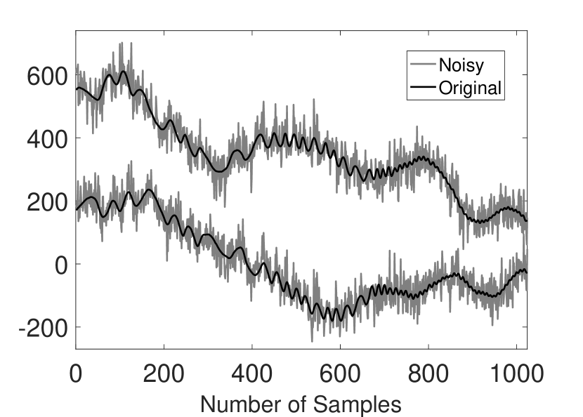
(a) Noisy at 10 dB

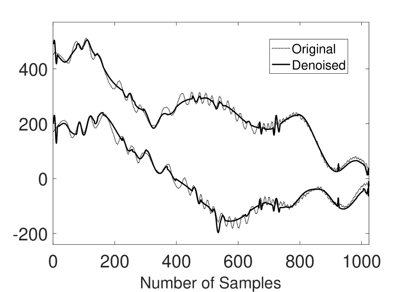
(b) MMD

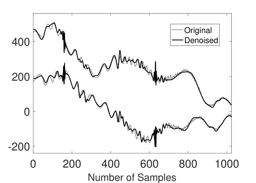
(c) MWD

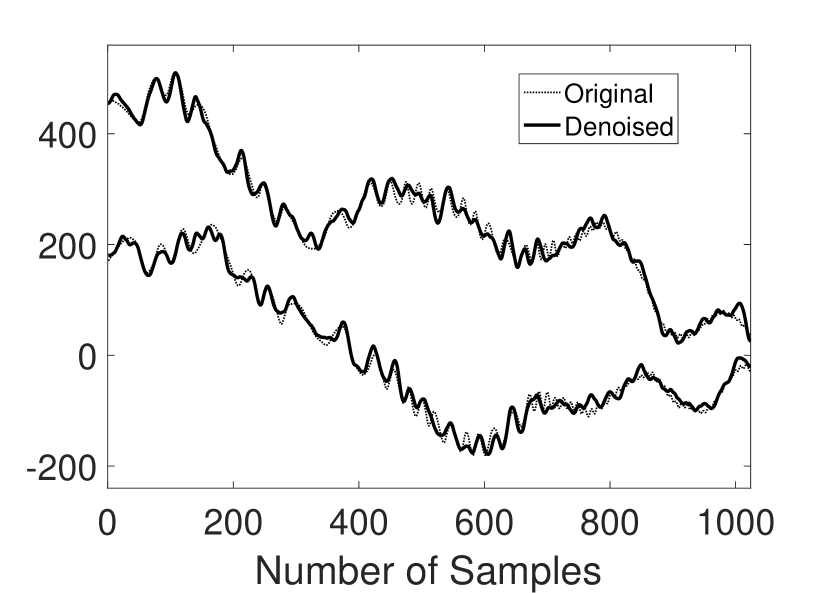
(d) Prop. MDD

Fig. 4: Comparison of visual denoising results of the proposed MDD method against the state of the art methods for real Sofar signal at input SNR $=10$ dB.

Table 1 reports average output SNRs for $J=20$ realizations from the comparative methods for all the input datasets (described above) at input SNR $=-2,2,6$ and $10$ dB. At each input noise level, we consider balanced noise (i.e., same input SNRs for all channels) and unbalanced noise cases (i.e., different input SNRs across different channels). To accentuate the best performing method, highest output SNRs are highlighted in bold for each input SNR. Observe that in most cases, the proposed MDD method yields highest output SNRs demonstrating the effectiveness of our method. Occasionally, at higher output SNRs, MMD outperforms our MDD method while MWD - generally regarded as a benchmark in multichannel signal denoising - remains competitive as well.

Finally, we inspect the visual quality of the reconstructed signal by displaying the denoised Sofar signals in Fig. 4 along with the noisy version at input SNR $=10$ dB. For meaningful qualitative analysis, we plotted original signal (shown using dotted line) in the background of the denoised signals (shown using solid line) in each case. Evidently, proposed MDD method yields best estimate of the original signal since it can estimate subtle details along with the slow variations, see Fig. 4 (d). On the contrary, MMD and MWD not only miss important signal details but also yield artifacts.

5 Conclusion

We have proposed a novel multivariate signal denoising method that is based on multiscale data representation and statistical signal properties. A novel and generic multichannel extension of detrended fluctuation analysis (DFA) underpins our denoising method which has been shown to outperform existing approaches owing to the full utilization of interchannel correlations within input data through utilization of Mahalanobis distance measure.

References

- [1] David L Donoho, Iain M Johnstone, Gérard Kerkyacharian, and Dominique Picard, “Wavelet shrinkage: asymptopia?,” Journal of the Royal Statistical Society. Series B (Methodological), pp. 301–369, 1995.
- [2] Alireza Ahrabian and Danilo P Mandic, “A class of multivariate denoising algorithms based on synchrosqueezing.,” IEEE Trans. Signal Processing, vol. 63, no. 9, pp. 2196–2208, 2015.
- [3] Huan Hao, HL Wang, and NU Rehman, “A joint framework for multivariate signal denoising using multivariate empirical mode decomposition,” Signal Processing, vol. 135, pp. 263–273, 2017.
- [4] Naveed ur Rehman, Bushra Khan, and Khuram Naveed, “Data-driven multivariate signal denoising using mahalanobis distance,” IEEE Signal Processing Letters, vol. 26, no. 9, pp. 1408–1412, 2019.
- [5] Khuram Naveed and Naveed ur Rehman, “Wavelet based multivariate signal denoising using mahalanobis distance and edf statistics,” IEEE Transactions on Signal Processing, vol. 68, pp. 5997–6010, 2020.
- [6] Sylvain Meignen, Thomas Oberlin, and Stephen McLaughlin, “A new algorithm for multicomponent signals analysis based on synchrosqueezing: With an application to signal sampling and denoising,” IEEE transactions on Signal Processing, vol. 60, no. 11, pp. 5787–5798, 2012.
- [7] Yannis Kopsinis and Stephen McLaughlin, “Development of emd-based denoising methods inspired by wavelet thresholding,” IEEE Transactions on signal Processing, vol. 57, no. 4, pp. 1351–1362, 2009.
- [8] Naveed ur Rehman, Syed Zain Abbas, Anum Asif, Anum Javed, Khuram Naveed, and Danilo P Mandic, “Translation invariant multi-scale signal denoising based on goodness-of-fit tests,” Signal Processing, vol. 131, pp. 220–234, 2017.
- [9] Naveed ur Rehman, Khuram Naveed, Shoaib Ehsan, and Klaus McDonald-Maier, “Multi-scale image denoising based on goodness of fit (gof) tests,” in 2016 24th European Signal Processing Conference (EUSIPCO). IEEE, 2016, pp. 1548–1552.
- [10] Konstantin Dragomiretskiy and Dominique Zosso, “Variational mode decomposition,” IEEE transactions on signal processing, vol. 62, no. 3, pp. 531–544, 2014.
- [11] Naveed ur Rehman and Hania Aftab, “Multivariate variational mode decomposition,” IEEE Transactions on Signal Processing, vol. 67, no. 23, pp. 6039–6052, 2019.
- [12] Yuanyuan Liu, Gongliu Yang, Ming Li, and Hongliang Yin, “Variational mode decomposition denoising combined the detrended fluctuation analysis,” Signal Processing, vol. 125, pp. 349–364, 2016.
- [13] Khuram Naveed, Muhammad Tahir Akhtar, Muhammad Faisal Siddiqui, and Naveed ur Rehman, “A statistical approach to signal denoising based on data-driven multiscale representation,” Digital Signal Processing, vol. 108, pp. 102896, 2021.
- [14] Peipei Cao, Huali Wang, and Kaijie Zhou, “Multichannel signal denoising using multivariate variational mode decomposition with subspace projection,” IEEE Access, vol. 8, pp. 74039–74047, 2020.
- [15] C-K Peng, Sergey V Buldyrev, Shlomo Havlin, Michael Simons, H Eugene Stanley, and Ary L Goldberger, “Mosaic organization of dna nucleotides,” Physical review e, vol. 49, no. 2, pp. 1685, 1994.
- [16] Hui Xiong and Pengjian Shang, “Detrended fluctuation analysis of multivariate time series,” Communications in Nonlinear Science and Numerical Simulation, vol. 42, pp. 12–21, 2017.
- [17] Jan W Kantelhardt, Eva Koscielny-Bunde, Henio HA Rego, Shlomo Havlin, and Armin Bunde, “Detecting long-range correlations with detrended fluctuation analysis,” Physica A: Statistical Mechanics and its Applications, vol. 295, no. 3-4, pp. 441–454, 2001.
- [18] Ahmet Mert and Aydin Akan, “Detrended fluctuation thresholding for empirical mode decomposition based denoising,” Digital Signal Processing, vol. 32, pp. 48–56, 2014.
- [19] Samuel Leistedt, Martine Dumont, J-P Lanquart, Fabrice Jurysta, and Paul Linkowski, “Characterization of the sleep eeg in acutely depressed men using detrended fluctuation analysis,” Clinical neurophysiology, vol. 118, no. 4, pp. 940–950, 2007.
- [20] Mina Aminghafari, Nathalie Cheze, and Jean-Michel Poggi, “Multivariate denoising using wavelets and principal component analysis,” Computational Statistics & Data Analysis, vol. 50, no. 9, pp. 2381–2398, 2006.
- [21] Dimitris Karlis, Gilbert Saporta, and Antonis Spinakis, “A simple rule for the selection of principal components,” Communications in Statistics-Theory and Methods, vol. 32, no. 3, pp. 643–666, 2003.
- [22] PL Richardson, JF Price, D Walsh, L Armi, and M Schröder, “Tracking three meddies with sofar floats,” Journal of Physical Oceanography, vol. 19, no. 3, pp. 371–383, 1989.
- [23] K Naveed, “Multivariate signal denoising using generic multichannel dfa,” 2020, [Online], Matlab Central File Exchange, vol. https://www.mathworks.com/matlabcentral/fileexchange/78062-multivariate-signal-denoising-using-generic-multichannel-dfa.