BUNET: Blind Medical Image Segmentation Based on Secure UNET

Abstract

The strict security requirements placed on medical records by various privacy regulations become major obstacles in the age of big data. To ensure efficient machine learning as a service schemes while protecting data confidentiality, in this work, we propose blind UNET (BUNET), a secure protocol that implements privacy-preserving medical image segmentation based on the UNET architecture. In BUNET, we efficiently utilize cryptographic primitives such as homomorphic encryption and garbled circuits (GC) to design a complete secure protocol for the UNET neural architecture. In addition, we perform extensive architectural search in reducing the computational bottleneck of GC-based secure activation protocols with high-dimensional input data. In the experiment, we thoroughly examine the parameter space of our protocol, and show that we can achieve up to 14x inference time reduction compared to the-state-of-the-art secure inference technique on a baseline architecture with negligible accuracy degradation.

1 Introduction

The use of neural-network (NN) based machine learning (ML) algorithms in aiding medical diagnosis, especially in the field of medical image computing, appears to be extremely successful in terms of its prediction accuracy. However, the security regulations over medical records contradicts the use of big data in the age of ML. Highly sensitive patient records are protected under the Health Insurance Portability and Accountability Act (HIPAA), where strong protection measures need to be taken over all of the electronic Protected Health Information (ePHI) possessed by a patient. In particular, access controls and client-side encryption are mandated for the distribution of all ePHI records over public networks [14, 12]. In addition, while qualified professionals are allowed to handle ePHI, the data exposure is required to be kept minimal [10, 13], i.e., just enough to accomplish the necessary professional judgements.

A central question to the real-world deployment of NN-based ML techniques in medical image processing is how the related data transfer and computations can be handled securely and efficiently. Previous security measures on medical data generally involved physical means (e.g., physically disconnected from the internet), and these techniques clearly cannot benefit from the large-scale distributed computing networks available for solving ML tasks. Recent advances in cryptography and multi-party secure computing seek alternatives to address the security concerns. In particular, the concept of secure inference (SI) is proposed, where Alice as a client wishes to inference on some of her inputs with the machine learning models provided by the server, called Bob. The security requirement is that no one, including Bob, learns anything about the inputs from Alice, while Alice also learns nothing about the models from Bob. Over the past few years, prior arts on SI flourished [17, 18, 24, 15, 22, 6], where secure protocols targeted on general learning problems were proposed. In addition, we also observe protocol- and system-level optimizations [22, 2] on SI. Unfortunately, most existing works mentioned above do not have a clear application in mind. Thus, the utilized network architectures and datasets (e.g., MNIST, CIFAR-10) are usually generic, without immediate practical implications.

In this work, we propose BUNET, a secure protocol for the UNET architecture [23] that enables input-hiding segmentation on medical images. In the proposed protocol, we use a combination of cryptographic building blocks to ensure that client-side encryption is enforced on all data related to the patients, and that practical inference time can also be achieved. As a result, medical institutions can take advantage of third-party machine learning service providers without violating privacy regulations. The main contributions of this work are summarized as follows.

• Privacy-Preserving Image Segmentation: To the best of our knowledge, we are the first to propose a secure protocol for image segmentation.

• Architectural Exploration for Secure UNET: We perform a search on the possible alternative UNET architectures to reduce the amount of computations (in terms of cryptographic realizations) in SI.

• Thorough Empirical Evaluations: By performing architectural-protocol co-design, we achieved 8x–14x inference time reduction with negligible accuracy degradation.

2 Preliminaries

2.1 Cryptographic Primitives

In this work, we mainly consider the four types of cryptographic primitives: a packed additive homomorphic encryption (PAHE) scheme based on the ring learning with errors (RLWE) problem [4, 11, 5, 8], additive secret sharing (ASS) [9], garbled circuits (GC) [26], and multiplication triples (MT) [1, 16]. In what follows, we provide a brief overview for each primitive.

PAHE: A PAHE is a cryptosystem, where the encryption ($\operatorname{\mathsf{Enc}}$) and decryption ($\operatorname{\mathsf{Dec}}$) functions act as group (additive) homomorphisms between the plaintext and ciphertext spaces. Except for the normal $\operatorname{\mathsf{Enc}}$ and $\operatorname{\mathsf{Dec}}$, a PAHE scheme is equipped with the following three abstract operators. We use $[{\bf{x}}]$ to denote the encrypted ciphertext of ${\bf{x}}\in{\mathbb{Z}}^{n}$, and $n\in{\mathbb{Z}}$ the maximum number of plaintext integers that can be held in a single ciphertext.

• Homomorphic addition $(\boxplus)$: for ${\bf{x}},{\bf{y}}\in{\mathbb{Z}}^{n}$, $\operatorname{\mathsf{Dec}}([{\bf{x}}]\boxplus[{\bf{y}}])={\bf{x}}+{\bf{y}}$. Note we can also perform homomorphic subtraction $\boxminus$, where $\operatorname{\mathsf{Dec}}([{\bf{x}}]\boxminus[{\bf{y}}])={\bf{x}}-{\bf{y}}$.

• Homomorphic Hadamard product $(\boxcircle)$: for ${\bf{x}},{\bf{y}}\in{\mathbb{Z}}^{n}$, $\operatorname{\mathsf{Dec}}([{\bf{x}}]\boxcircle{\bf{y}})={\bf{x}}\circ{\bf{y}}$, where $\circ$ is the element-wise multiplication operator.

• Homomorphic rotation $({\mathsf{rot}})$: for ${\bf{x}}\in{\mathbb{Z}}^{n}$, let ${\bf{x}}=(x_{0},x_{1},\cdots,x_{n-1})$, ${\mathsf{rot}}([{\bf{x}}],k)=(x_{k},x_{k+1},\cdots,x_{n-1},x_{0},\cdots,x_{k-1})$ for $k\in\{0,\cdots,n-1\}$.

ASS and Homomorphic Secret Sharing: A two-party ASS scheme consists of two operators, $(\mathsf{Share},\mathsf{Rec})$, and some prime modulus $p_{\rm A}\in{\mathbb{Z}}$. Each operator takes two inputs, where we have ${\bf{s}}_{A}=\mathsf{Share}({\bf{x}},{\bf{s}}_{B})=({\bf{x}}-{\bf{s}}_{B})\bmod{p_{\rm A}}$ and ${\bf{x}}=\mathsf{Rec}({\bf{s}}_{A},{\bf{s}}_{B})=({\bf{s}}_{A}+{\bf{s}}_{B})\bmod{p_{\rm A}}$. In [15], homomorphic secret sharing (HSS) is adopted, where ASS operates over an encrypted ${\bf{x}}$. For HSS, we have that

$$[{\bf{s}}_{A}] =\mathsf{Share}([{\bf{x}}],{\bf{s}}_{B})=([{\bf{x}}]\boxminus{\bf{s}}_{B})\bmod{p_{\rm A}}\text{, and }$$ (1)

$$[{\bf{x}}] =\mathsf{Rec}([{\bf{s}}_{A}],{\bf{s}}_{B})=({\bf{s}}_{A}\boxplus{\bf{s}}_{B})\bmod{p_{\rm A}}.$$ (2)

GC: GC can be considered as a more general form of HE. In particular, the circuit garbler, Alice, “encrypts” some function $f$ along with her input $x$ to Bob, the circuit evaluator. Bob evaluates $f(x,y)$ using his encrypted input $y$ that is received from Alice obliviously, and obtains the encrypted outputs. Alice and Bob jointly “decrypt” the output of the function $f(x,y)$ and one of the two parties learns the result.

MT: Beaver’s MT [1] is a technique that performs multiplication on a pair of secret-shared vectors ${\bf{x}}=\mathsf{Rec}({\bf{s}}_{A,x},{\bf{s}}_{B,x})$ and ${\bf{y}}=\mathsf{Rec}({\bf{s}}_{A,y}+{\bf{s}}_{B,y})$ between Alice and Bob. Here, we take computations performed by Alice as an example, and only note that the exact same procedure is also executed by Bob on his shares of secrets. To compute ${\bf{x}}\circ{\bf{y}}$, Alice and Bob first pre-share a set of respective multiplication triples $({\bf{a}}_{A},{\bf{b}}_{A},{\bf{c}}_{A})$ and $({\bf{a}}_{B},{\bf{b}}_{B},{\bf{c}}_{B})$, where we have $\mathsf{Rec}({\bf{a}}_{A},{\bf{a}}_{B})\circ\mathsf{Rec}({\bf{b}}_{A},{\bf{b}}_{B})=\mathsf{Rec}({\bf{c}}_{A},{\bf{c}}_{B})$. Alice locally calculates ${\bf{d}}_{A}={\bf{s}}_{A,x}\circ{\bf{a}}_{A}\bmod{p_{\rm A}},{\bf{e}}_{A}={\bf{b}}_{A}\circ{\bf{s}}_{A,y}\bmod{p_{\rm A}}$. Then, Alice and Bob publish their results ${\bf{d}}_{A},{\bf{d}}_{B}$ and ${\bf{e}}_{A},{\bf{e}}_{B}$. Finally, Alice obtains

$${\bf{g}}_{A}=\big{(}{\bf{c}}_{A}+({\bf{e}}\circ{\bf{s}}_{A,0,i})+({\bf{d}}\circ{\bf{s}}_{A,1,i})-{\bf{d}}\circ{\bf{e}}\big{)}\bmod{p_{\rm A}},$$ (3)

where ${\bf{d}}=\mathsf{Rec}({\bf{d}}_{A},{\bf{d}}_{B})$ and similarly for ${\bf{e}}$. MT guarantees that $\mathsf{Rec}({\bf{g}}_{A},{\bf{g}}_{B})={\bf{x}}\circ{\bf{y}}$, where ${\bf{g}}_{B}$ is the MT results computed by Bob.

2.2 Related Works on Secure Neural Network Inference

While a limited number of pioneering works have been proposed for secure inference and training with neural networks [17, 18, 24, 15], it was not until recently that such protocols carried practical significance. For example, in [17], an inference with a single CIFAR-10 image takes more than 500 seconds to complete. Using the same neural architecture, the performance was improved to less than 8 seconds in one of the most recent arts on SI, ENSEI [15]. Unfortunately, as shown in Section 4, without UNET-specific optimizations and protocol designs, existing approaches carry significant performance overhead, especially on the 3D images (e.g., CT scans) used in medical applications. Hence, in this work, we establish our protocol based on the ENSEI construction, and explore UNET-specific optimizations and cryptographic protocol designs to improve the practicality of secure inference in medical segmentation.

3 Secure UNET for Blind Segmentation

3.1 BUNET: The Protocol

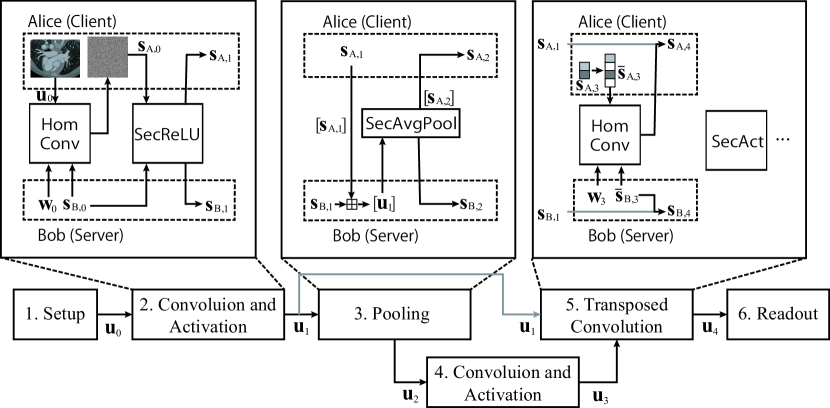
Figure 1: The overview of the BUNET protocol.

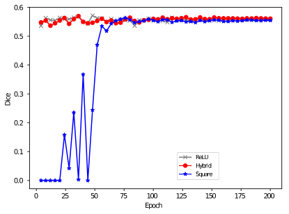
Figure 3: The learning curve for different neural architectures over 200 epoches. It can be observed that the neural architecture with all-square activation encounters some difficulties initially, but successfully proceeded learning later on.

Fig. 3 shows an example of the BUNET protocol structured as an UNET architecture, where the input image goes through four steps. The operators used in each step will be discussed in detail later in Section 3.2.

• Setup: As our protocol takes both 2D and 3D images as inputs, the input image is of dimension $\dim(U)=c\times w\times h\times d$ ($d=1$ for 2D inputs). Alice first raster-scans her input image into a one-dimensional vector ${\bf{u}}$ of length $\ell=c\cdot w\cdot h\cdot d$. Bob does a similar transformation on his filter weights to obtain the one-dimensional vector ${\bf{w}}$. We use ${\bf{u}}_{0}$ to denote the input from Alice at the $0$-th layer, and ${\bf{w}}_{0}$ for that of Bob.

• Convolution and Activation: We conduct a standard (input-hiding) convolution on the input image with activation functions followed. For each convolution layer with activation, we run

  $${\bf{v}}_{0}=\operatorname{\mathsf{HomConv}}({\bf{u}}_{0},{\bf{w}}_{0}),\text{ and }{\bf{u}}_{1}=f_{a}({\bf{v}}_{0})=\operatorname{\mathsf{SecAct}}({\bf{v}}_{0}).$$ (4)

  for some weight vector ${\bf{w}}_{0}$. Here, $f_{a}$ is some abstract activation function (e.g., ReLU or square activation). The output ${\bf{u}}_{1}=f_{a}({\bf{v}}_{0})$ will become the input to the next layer. We point out that the activation function has a significant impact on both the accuracy and the inference time of UNET. Therefore, we propose a hybrid UNET architecture, where both ReLU and square activations are used. Here, the security guarantee is that Alice obtains no knowledge on ${\bf{w}}_{0}$, and Bob knows nothing about ${\bf{u}}_{0}$ and ${\bf{v}}_{0}$ after the protocol execution.

• Pooling: While the standard UNET architecture employs max pooling [23] as the downsampling method, in the experiment, we show a large performance difference between max pooling and average pooling protocols, due to the change of underlying protocol. We also demonstrate in Table 4 that the two pooling methods result in marginal accuracy differences. Hence, we modified the UNET architecture to employ only average pooling. Consequently, the proposed protocol executes ${\bf{u}}_{2}=\operatorname{\mathsf{SecAvgPool}}({\bf{u}}_{1})$. For an input of length $\ell$ and pooling size $\zeta_{p}=z_{w,p}\times z_{h,p}\times z_{d,p}$, the pooled output have a dimension of $\ell/\zeta_{p}$.

• Bottom-Level Convolution and Activation: Here, Step 2 is repeated, and we get ${\bf{u}}_{3}$ as output. Note that the input and output dimension is reduced by Step 3, so Step 4 is computationally lighter than Step 2.

• Transposed Convolution and Concatenation: While the arithmetic procedures for transposed convolution is essentially the same as a normal convolution, protocol-level modifications are required for the image concatenation and padding operations. Concretely, after obtaining input from the previous layer, e.g., ${\bf{u}}_{3}$, Alice needs to zero-pad ${\bf{u}}_{3}$ in an interleaving manner, according to some stride size $\zeta_{t}=z_{w,t}\times z_{h,t}\times z_{d,t}$. The padded result, ${\overline{{\bf{u}}}}_{3}$, will have a length of $\ell\cdot\zeta_{t}/\zeta_{p}$. Subsequently, Alice uses ${\overline{{\bf{u}}}}_{3}$ as input to execute the following protocols.

  $${\bf{v}}_{4}=\operatorname{\mathsf{HomConv}}({\overline{{\bf{u}}}}_{3},{\bf{w}}_{3}),\text{ and }{\bf{u}}_{4}={\bf{v}}_{4}||{\bf{u}}_{1}.$$ (5)

  One subtlety is that, the output from the $1$-st layer, ${\bf{u}}_{1}$, needs to be concatenated with the output from the transposed convolution layer for the rest of the normal convolutions. However, ${\bf{u}}_{1}$ and ${\bf{v}}_{4}$ will actually be encrypted under different keys. Thus, both results need to be decrypted and concatenated by Alice. The concatenated result, ${\bf{v}}_{1}||{\bf{u}}_{4}$, will become the inputs to later layers.

• Readout: Here, we applies the $\operatorname{\mathsf{SecArgmax}}$ function over the label dimensions. It is noted that, since the ${\mathsf{Softmax}}$ operator is monotonic and is only required in the learning process, we avoid using a separate protocol for ${\mathsf{Softmax}}$, and directly perform a secure ${\mathsf{Argmax}}$. Since the $\mathsf{Argmax}$ function is a pixel-wise comparison function across the label dimension, it can be implemented using a simple GC protocol similar to the secure ReLU protocol, and we omit a formal presentation.

3.1.1 Threat Model and Security

The threat model for BUNET is that both Bob and Alice are semi-honest, in the sense that both parties follow the protocol prescribed above (e.g., encrypting real data with $\operatorname{\mathsf{Enc}}$, etc.), but want to learn as much information as possible from the other party. Our protocol guarantees that Alice learns only the segmentation results, while Bob learns nothing about the inputs from Alice.

The security of the proposed protocol can be easily reduced to that of existing works [15, 3], where any attack against BUNET will result in a non-negligible advantage against the ENSEI [3] and Gazelle [15] protocols.

3.2 The Cryptographic Building Blocks

Here, we discuss each of the cryptographic primitives used in the previous section in details.

$\operatorname{\mathsf{HomConv}}$: The $\operatorname{\mathsf{HomConv}}$ operator obliviously convolve two vectors ${\bf{u}}$ and ${\bf{w}}$. A very recent work [3] discovered that, instead of the complex rotate-and-accumulate approach proposed by previous works [15], homomorphic convolution can be performed in the frequency domain, where the only computation needed in the homomorphic domain is the $\boxcircle$ (homomorphic Hadamard product) operator. Therefore, the homomorphic convolution protocol proceeds as follows.

• First, Alice performs an integer discrete Fourier transform (DFT) (i.e., number theoretic transform in [3]) on ${\bf{u}}$ and obtain its frequency-domain representation, ${\hat{{\bf{u}}}}$. She simply encrypts this input array into a ciphertext $[{\hat{{\bf{u}}}}]$ (when $\ell>n$, the vector is encrypted into multiple ciphertexts) by running $[{\hat{{\bf{u}}}}]=\operatorname{\mathsf{Enc}}_{{\mathcal{K}}}({\hat{{\bf{u}}}})$, where ${\mathcal{K}}$ is the encryption key. The resulting ciphertext is transferred to Bob.

• Before receiving any input from Alice, Bob applies DFT on his filter weights to obtain ${\hat{{\bf{w}}}}$. In this process, the size of the filter will be padded to be $\ell$. Upon receiving the inputs $[{\hat{{\bf{u}}}}]$ from Alice, Bob computes

  $$[{\hat{{\bf{v}}}}]=[{\hat{{\bf{u}}}}\circ{\hat{{\bf{w}}}}]=[{\hat{{\bf{u}}}}]\boxcircle{\hat{{\bf{w}}}}$$ (6)

  for all ciphertexts ${\hat{{\bf{u}}}}$.

• Finally, since ${\hat{{\bf{v}}}}$ contains information of the weights from Bob, Bob applies HSS as $[{\hat{{\bf{s}}}}_{A}]=\mathsf{Share}([{\hat{{\bf{v}}}}],{\hat{{\bf{s}}}}_{B})$. Bob keeps ${\hat{{\bf{s}}}}_{B}$ and returns $[{\hat{{\bf{s}}}}_{A}]$ to Alice, where Alice decrypts and obtain ${\hat{{\bf{s}}}}_{A}$. Both Alice and Bob run inverse DFT on their shares of secrets (i.e., ${\hat{{\bf{s}}}}_{A}$ and ${\hat{{\bf{s}}}}_{B}$) and obtain ${\bf{s}}_{A}$ and ${\bf{s}}_{B}$, respectively, completing the protocol.

$\operatorname{\mathsf{SecAct}}$: The $\operatorname{\mathsf{SecAct}}$ protocols are summarized as follows.

• ReLU: We follow the construction in [15] based on the GC protocol. Alice first garbles the circuit with her share of secret ${\bf{s}}_{A}$. The garbled circuit obliviously computes the following function

  $${\bf{v}}=\mathsf{Rec}({\bf{s}}_{A},{\bf{s}}_{B}),{\text{ and }}{\overline{{\bf{s}}}}_{A}=\mathsf{Share}(\mathsf{ReLU}({\bf{v}}),{\overline{{\bf{s}}}}_{B})$$ (7)

  where ${\overline{{\bf{s}}}}_{B}$ is a freshly generated share of secret from Bob. After protocol execution, Alice obtains ${\overline{{\bf{s}}}}_{A}$, which contains $\mathsf{ReLU}({\bf{v}})$ in an oblivious manner.

• Square: Since the square activation (i.e., $y=x^{2}$) is essentially evaluating a polynomial over the inputs, the computationally-light MT can be used instead of GC. To use MT, we first share the secret ${\bf{v}}$ twice among Alice and Bob. Then, the MT protocol outlined in Section 2.1 can be executed, where both ${\bf{x}}$ and ${\bf{y}}$ equal ${\bf{v}}$. After the protocol execution, Alice and Bob respectively obtain ${\bf{g}}_{A}$ and ${\bf{g}}_{B}$ where $\mathsf{Rec}({\bf{g}}_{A},{\bf{g}}_{B})={\bf{v}}^{2}$. The main observation here is that, all computations are coefficient-wise multiplications and additions over $\lg{p_{\rm A}}$-bit integers. As a result, MT-based square activation is much faster than GC-based ReLU activation.

$\mathsf{SecPool}$: As mentioned above, two types of secure pooling can be implemented, the $\mathsf{SecMaxPool}$ and the $\operatorname{\mathsf{SecAvgPool}}$ operator. In [15], it is shown that max-pooling can be implemented using the GC protocol as in Eq. (7), where we replace the $\mathsf{ReLU}$ operator with the $\mathsf{MaxPool}$ operator. Meanwhile, for secure average pooling, we can use a simple protocol that is purely based on PAHE. Specifically, we can compute the window-wise sum of some vector ${\bf{v}}$ by calculating $\operatorname{\mathsf{SecAvgPool}}({\bf{v}})=\sum_{i=0}^{\zeta_{p}-1}{\mathsf{rot}}([{\bf{v}}],i)$, where $\zeta_{p}$ is the pooling window size. Since both homomorphic rotations and additions are light operations compared to GC, $\operatorname{\mathsf{SecAvgPool}}$ is much faster than $\mathsf{SecMaxPool}$.

4 Accuracy Experiments and Protocol Instantiation

4.1 Experiment Setup

Due to the lack of immediate existing works, we compare BUNET with the standard UNET architecture implemented by the ENSEI [3] protocol, which is the best performing protocol on secure multi-class inference. Here, the standard UNET architecture only utilizes max-pooling for pooling layers, and ReLU for activation layers. We denote this architecture as the baseline architecture. As shown in the appendix, the baseline architecture consists 19 convolution layers including three transposed convolution layers, 14 activation layers, three average pooling layers, and a readout layer implementing the $\operatorname{\mathsf{SecArgmax}}$ function.

Our experiments are conducted on three datasets, GM [21], EM [7], and HVSMR [20]. Due to the space constraint, we only present the accuracy and performance results on the EM (two dimensional) and HVSMR (three dimensional) datasets (GM will be added to the appendix).

The cryptographic performance is characterized on an Intel i5-9400 2.9 GHz CPU, and the accuracy results are obtained with an NVIDIA P100 GPU. The adopted PAHE library is SEAL version 3.3.0 [25] (we set $q,p$ to be 60-bit and 20-bit integers, respectively, and $n=2048$, ensuring a 128-bit security) and MT/GC protocols are implemented using LowGear provided by MP-SPDZ [16, 19].

4.2 Accuracy and Performance Results

Table 1: The Dice Accuracy on the HVSMR Dataset for Different Neural Architectures

	ReLU+Max	ReLU	ReLU+Max	ReLU	Hybrid	Square
	Float	Float	32-bit (Baseline)	16-bit	20-bit	16-bit
HVSMR Myo. Dice	0.74$\pm 0.04$	0.73$\pm 0.04$	0.73$\pm 0.05$	0.73$\pm 0.05$	0.71$\pm 0.05$	0.52$\pm 0.14$
HVSMR BP Dice	0.87$\pm 0.04$	0.87$\pm 0.04$	0.87$\pm 0.04$	0.87$\pm 0.04$	0.86$\pm 0.05$	0.83$\pm 0.05$
HVSMR Time (s)	-	-	42616	14205	3054.2	1118.2
EM Dice	0.9405	-	0.9411	0.9398	0.9385	0.8767
EM Time (s)	-	-	8838.1	2968.6	1077.9	227.16

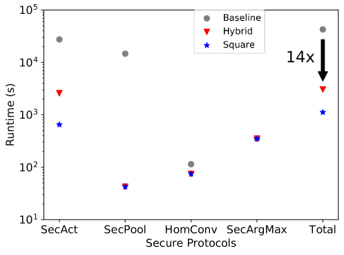
Figure 2: Runtime distribution for different cryptographic building blocks in a single run of secure segmentation.

Table 2: Number of Activation Functions per Layer Batch

1st	2nd	3rd	4th	5th	6th	7th
33554432	8388608	2097152	524288	2097152	8388608	33554432

In this section, we explore how the neural architecture of 3D-UNET impact on the segmentation performance. In particular, it is important to see if the the proposed architectural modifications for UNET result in satisfactory prediction accuracy while accelerating the network inference time. We downsampled the images in the HVSMR [20] dataset to a dimension of $64\times 64\times 64$ containing three class labels, i.e., background, myocardium (myo.) and blood pool (BP). The images in the EM dataset has $200\times 200$ input for binary segmentation. Table 4 summarizes the dice scores and runtime under various architectural settings (HVSMR with 10-fold cross validation). Here, the pooling function is average pooling unless otherwise stated. Hybrid refers to the neural architecture where the first and the last layer batches use square activation, while all other layer batches adopt ReLU activation. Here, a layer batch denotes two convolution and activation layers with the same output feature dimensions and channels. We have three main observations. First, the use of average pooling instead of max pooling results in negligible accuracy degradation, on a level that can likely be compensated by parameter tuning. Second, the UNET architecture is robust in low-quantization environment, where we see little accuracy difference between floating point, 32-bit and 16-bit quantization factors, especially on the EM dataset. Lastly, replacing all ReLU activations with squares results in significant accuracy degradation for the segmentation of myocardium. However, the BP prediction can be acceptable for a quick run of cheap evaluations, and the hybrid architecture successfully achieves a good balance between accuracy and performance.

We record the total runtime for a single blind image segmentation with respect to different 3-D UNET architectures. In Table 2 and Fig. 2, we illustrate the per-layer-batch number of neuron activations and the runtime distribution for different secure protocols in BUNET. As expected, the first and last two layers contain the most amount of activations, and replacing the GC-based heavy ReLU activation with square activation results in an immediate 5x total runtime reduction. In addition, it is observed that the runtime for ReLU activation functions dominate the total runtime across architectures, while square activation is as light as a frequency-domain homomorphic convolution operation.

Compared to the baseline 32-bit ReLU architecture, we obtain 8x–14x runtime reduction with the reasonably accurate Hybrid architecture, and up to 39x reduction with the cheapest (all-square) UNET implementation on EM. Finally, we note that most NN operations can be parallelized as well as the cryptographic building blocks. Therefore, since our performance is recorded on a single-thread CPU, we expect further runtime reduction for BUNET on parallel computing architectures.

5 Conclusion

In this work, we propose BUNET to perform blind medical image segmentation on encrypted medical images. The observation we make is that protocol and network designs need to be jointly performed to achieve the best accuracy-performance trade-off. By designing UNET-specific protocols and optimizing the UNET architecture, we show that up to 8x–14x inference time reduction can be achieved with negligible accuracy degradation on several medical datasets.

Appendix for BUNET: Blind Medical Image Segmentation Based on Secure UNET

Song Bian Xiaowei Xu Weiwen Jiang Yiyu Shi Takashi Sato

6 Additional Experiment Results for EM/GM datasets

Table 3: The Dice Accuracy and Runtime for the GM Dataset for Different Neural Architectures. Note that since we have the same architecture and input dimensions for GM and EM, the runtime for the secure inference protocol is the same.

	ReLU+Max	ReLU	ReLU+Max	ReLU	Hybrid	Square
	Float	Float	32-bit (Baseline)	16-bit	16-bit	16-bit
GM Dice	0.5632	-	0.5581	0.5577	0.5607	0.5546
GM Time (s)	-	-	8838.1	2968.6	1077.9	227.16

7 Detailed Network Architecture

Table 4: The neural architecture for the 3-D UNET used in HVSMR dataset. The input is of dimension $1\times 64\times 64\times 64=64^{3}$ where $1$ denotes a single channel. For EM and GM, we replace the input dimension $64^{3}$ with $200^{2}$, and the filter dimensions are kept the same. Here, Quant. and Quantization indicate a quantization layer that quantize all the outputs from the previous operation (e.g., convolution or square activation). Meanwhile, Norm. denotes a normalization layer.

Layer Batch	Layer Type	Input Dim.	Filter Dim.	Output Dim.
1	Convolution+Quant.	$1\times 64^{3}$	$64\times 3^{3}$	$64\times 64^{3}$
1	Activation+Norm.	$64\times 64^{3}$	-	$64\times 64^{3}$
1	Quantization	$64\times 64^{3}$	-	$64\times 64^{3}$
1	Convolution+Quant.	$64\times 64^{3}$	$64\times 3^{3}$	$64\times 64^{3}$
1	Activation+Norm.	$64\times 64^{3}$	-	$64\times 64^{3}$
1	Quantization	$64\times 64^{3}$	-	$64\times 64^{3}$
1	Pooling	$64\times 64^{3}$	$2^{3}$	$64\times 32^{3}$
2	Convolution+Quant.	$64\times 32^{3}$	$128\times 3^{3}$	$128\times 32^{3}$
2	Activation+Norm.	$128\times 32^{3}$	-	$128\times 32^{3}$
2	Quantization	$128\times 32^{3}$	-	$128\times 32^{3}$
2	Convolution+Quant.	$128\times 32^{3}$	$128\times 3^{3}$	$128\times 32^{3}$
2	Activation+Norm.	$128\times 32^{3}$	-	$128\times 32^{3}$
2	Quantization	$128\times 32^{3}$	-	$128\times 32^{3}$
2	Pooling	$128\times 32^{3}$	$2^{3}$	$128\times 16^{3}$
3	Convolution+Quant.	$128\times 16^{3}$	$256\times 3^{3}$	$256\times 16^{3}$
3	Activation+Norm.	$256\times 16^{3}$	-	$256\times 16^{3}$
3	Quantization	$256\times 16^{3}$	-	$256\times 16^{3}$
3	Convolution+Quant.	$256\times 16^{3}$	$256\times 3^{3}$	$256\times 16^{3}$
3	Activation+Norm.	$256\times 16^{3}$	-	$256\times 16^{3}$
3	Quantization	$256\times 16^{3}$	-	$256\times 16^{3}$
3	Pooling	$256\times 16^{3}$	$2^{3}$	$256\times 8^{3}$
4	Convolution+Quant.	$256\times 8^{3}$	$512\times 3^{3}$	$512\times 8^{3}$
4	Activation+Norm.	$512\times 8^{3}$	-	$512\times 8^{3}$
4	Quantization	$512\times 8^{3}$	-	$512\times 8^{3}$
4	Convolution+Quant.	$512\times 8^{3}$	$512\times 3^{3}$	$512\times 8^{3}$
4	Activation+Norm.	$512\times 8^{3}$	-	$512\times 8^{3}$
4	Quantization	$512\times 8^{3}$	-	$512\times 8^{3}$
4	Transposed Convolution+Quant.	$512\times 8^{3}$	$256\times 2^{3}$	$256\times 16^{3}$
5	Convolution+Quant.	$512\times 16^{3}$	$256\times 3^{3}$	$256\times 16^{3}$
5	Activation+Norm.	$256\times 16^{3}$	-	$256\times 16^{3}$
5	Quantization	$256\times 16^{3}$	-	$256\times 16^{3}$
5	Convolution+Quant.	$256\times 16^{3}$	$256\times 3^{3}$	$256\times 16^{3}$
5	Activation+Norm.	$256\times 16^{3}$	-	$256\times 16^{3}$
5	Quantization	$256\times 16^{3}$	-	$256\times 16^{3}$
5	Transposed Convolution+Quant.	$256\times 16^{3}$	$128\times 2^{3}$	$128\times 32^{3}$
6	Convolution+Quant.	$256\times 32^{3}$	$128\times 3^{3}$	$128\times 32^{3}$
6	Activation+Norm.	$128\times 32^{3}$	-	$128\times 32^{3}$
6	Quantization	$128\times 32^{3}$	-	$128\times 32^{3}$
6	Convolution+Quant.	$128\times 32^{3}$	$128\times 3^{3}$	$128\times 32^{3}$
6	Activation+Norm.	$128\times 32^{3}$	-	$128\times 32^{3}$
6	Quantization	$128\times 32^{3}$	-	$128\times 32^{3}$
6	Transposed Convolution+Quant.	$128\times 32^{3}$	$64\times 2^{3}$	$64\times 64^{3}$
7	Convolution+Quant.	$128\times 64^{3}$	$64\times 3^{3}$	$64\times 64^{3}$
7	Activation+Norm.	$64\times 64^{3}$	-	$64\times 64^{3}$
7	Quantization	$64\times 64^{3}$	-	$64\times 64^{3}$
7	Convolution+Quant.	$64\times 64^{3}$	$64\times 3^{3}$	$64\times 64^{3}$
7	Activation+Norm.	$64\times 64^{3}$	-	$64\times 64^{3}$
7	Quantization	$64\times 64^{3}$	-	$64\times 64^{3}$
8	Convolution	$64\times 64^{3}$	$3\times 3^{3}$	$3\times 64^{3}$
9	Argmax	$3\times 64^{3}$	-	$1\times 64^{3}$

References

- [1] Beaver, D.: Efficient multiparty protocols using circuit randomization. In: Annual International Cryptology Conference. pp. 420–432. Springer (1991)
- [2] Bian, S., Jiang, W., Lu, Q., Shi, Y., Sato, T.: NASS: Optimizing secure inference via neural architecture search. arXiv preprint arXiv:2001.11854 (2020)
- [3] Bian, S., Wang, T., Hiromoto, M., Shi, Y., Sato, T.: ENSEI: Efficient secure inference via frequency-domain homomorphic convolution for privacy-preserving visual recognition (2020)
- [4] Brakerski, Z.: Fully homomorphic encryption without modulus switching from classical GapSVP. In: Advances in Cryptology–CRYPTO 2012, pp. 868–886. Springer (2012)
- [5] Brakerski, Z., Gentry, C., Vaikuntanathan, V.: (Leveled) fully homomorphic encryption without bootstrapping. ACM Transactions on Computation Theory (TOCT) 6(3), 13 (2014)
- [6] Brutzkus, A., Gilad-Bachrach, R., Elisha, O.: Low latency privacy preserving inference. In: International Conference on Machine Learning. pp. 812–821 (2019)
- [7] Cardona, A., Saalfeld, S., Preibisch, S., Schmid, B., Cheng, A., Pulokas, J., Tomancak, P., Hartenstein, V.: An integrated micro-and macroarchitectural analysis of the drosophila brain by computer-assisted serial section electron microscopy. PLoS biology 8(10) (2010)
- [8] Cheon, J.H., Kim, A., Kim, M., Song, Y.: Homomorphic encryption for arithmetic of approximate numbers. In: International Conference on the Theory and Application of Cryptology and Information Security. pp. 409–437. Springer (2017)
- [9] Damgård, I., Nielsen, J.B., Polychroniadou, A., Raskin, M.: On the communication required for unconditionally secure multiplication. In: Annual International Cryptology Conference. pp. 459–488. Springer (2016)
- [10] Drolet, B.C., Marwaha, J.S., Hyatt, B., Blazar, P.E., Lifchez, S.D.: Electronic communication of protected health information: privacy, security, and hipaa compliance. The Journal of hand surgery 42(6), 411–416 (2017)
- [11] Fan, J., Vercauteren, F.: Somewhat practical fully homomorphic encryption. IACR Cryptology ePrint Archive 2012, 144 (2012)
- [12] HHS.gov: https://www.hhs.gov/hipaa/for-professionals/privacy/laws-regulations/index.html (2009), accessed: 2020-03-04
- [13] HHS.gov: https://www.hhs.gov/hipaa/for-professionals/privacy/guidance/minimum-necessary-requirement/index.html (2009), accessed: 2020-03-04
- [14] Hoffman, S., Podgurski, A.: Securing the hipaa security rule. Journal of Internet Law, Spring pp. 06–26 (2007)
- [15] Juvekar, C., et al.: Gazelle: A low latency framework for secure neural network inference. arXiv preprint arXiv:1801.05507 (2018)
- [16] Keller, M., Pastro, V., Rotaru, D.: Overdrive: making spdz great again. In: Annual International Conference on the Theory and Applications of Cryptographic Techniques. pp. 158–189. Springer (2018)
- [17] Liu, J., et al.: Oblivious neural network predictions via MinioNN transformations. In: Proc. of ACM SIGSAC Conference on Computer and Communications Security. pp. 619–631. ACM (2017)
- [18] Mohassel, P., et al.: Secureml: A system for scalable privacy-preserving machine learning. In: Proc. of Security and Privacy (SP). pp. 19–38. IEEE (2017)
- [19] MP-SPDZ: https://github.com/data61/MP-SPDZ/ (2018), accessed: 2020-03-10
- [20] Pace, D.F., Dalca, A.V., Geva, T., Powell, A.J., Moghari, M.H., Golland, P.: Interactive whole-heart segmentation in congenital heart disease. In: International Conference on Medical Image Computing and Computer-Assisted Intervention. pp. 80–88. Springer (2015)
- [21] Prados, F., Ashburner, J., Blaiotta, C., Brosch, T., Carballido-Gamio, J., Cardoso, M.J., Conrad, B.N., Datta, E., Dávid, G., De Leener, B., et al.: Spinal cord grey matter segmentation challenge. Neuroimage 152, 312–329 (2017)
- [22] Riazi, M.S., Samragh, M., Chen, H., Laine, K., Lauter, K.E., Koushanfar, F.: Xonn: Xnor-based oblivious deep neural network inference. IACR Cryptology ePrint Archive 2019, 171 (2019)
- [23] Ronneberger, O., Fischer, P., Brox, T.: U-net: Convolutional networks for biomedical image segmentation. In: International Conference on Medical image computing and computer-assisted intervention. pp. 234–241. Springer (2015)
- [24] Rouhani, B.D., et al.: Deepsecure: Scalable provably-secure deep learning. In: Proc. of DAC. pp. 1–6. IEEE (2018)
- [25] Microsoft SEAL (release 3.3). https://github.com/Microsoft/SEAL (June 2019), microsoft Research, Redmond, WA.
- [26] Yao, A.C.: Protocols for secure computations. In: Foundations of Computer Science, 1982. SFCS’08. 23rd Annual Symposium on. pp. 160–164. IEEE (1982)