Goal-oriented anisotropic $hp$-adaptive discontinuous Galerkin method for the Euler equations

Abstract

We deal with the numerical solution of the compressible Euler equations with the aid of the discontinuous Galerkin (DG) method with focus on the goal-oriented error estimates and adaptivity. We analyze the adjoint consistency of the DG scheme where the dual problem is not formulated by the differentiation of the DG form and the target functional but using a suitable linearization of the nonlinear forms. Further, we present the goal-oriented anisotropic $hp$-mesh adaptation technique for the Euler equations. The theoretical results are supported by numerical experiments.

1 Introduction

The motion of inviscid compressible fluids is described by the Euler equations whose efficient numerical solution is still a challenging problem. Among the prominent methods belongs the discontinuous Galerkin method (DGM) which exhibits an efficient technique for the numerical solution of various partial differential equations (PDEs). This paper looks into the solution of the Euler equations by DGM with focus on the goal-oriented (or output-based) error estimators and the mesh adaptivity. The aim is the approximation of a quantity of interest (e.g., the aerodynamics coefficients) given by a target functional depending on the solution of the problem considered.

The framework of the goal-oriented error estimates is already very-well established approach namely for linear PDEs, cf. surveys in RannacherBook ; BeckerRannacher01 ; GileSuli02 . This technique is based on the formulation of an adjoint problem whose solution appears as a weight of the primal residuals. For a nonlinear PDE (and a nonlinear target functional), the corresponding adjoint problem has to be derived for a linearized primal problem. The linearization is carried out by a differentiation of the primal formulation with respect to its approximate solution, see RannacherBook ; BeckerRannacher01 ; GileSuli02 for a general framework and, e.g., Hartmann2006Derivation ; HH06:SIPG2 ; LoseilleDervieuxAlauzet_JCP10 ; ceze:2013aniso ; BalanWoopenMay16 for applications of this approach to compressible flow problems. A comprehensive review of goal-oriented error estimates and mesh adaptation in computational fluid dynamics is given in FidkowskiDarmofal_AIAA11 .

Let ${a_{h}}$ be a semi-linear form representing the discretization of the given (nonliner) PDE, then the approximate solution ${{u}_{h}}\in V_{h}$ is defined by

$${a_{h}}({{u}_{h}},\varphi_{h})=0\qquad\forall\varphi_{h}\in V_{h},$$ (1)

where $V_{h}$ is a finite element space. Further, let $J$ be the target functional defining the quantity of interest $J(u)$ where $u$ is the exact solution. In order to estimate the error $J(u)-J({{u}_{h}})$, we introduce the adjoint (or dual) problem

$${a_{h}^{\prime}}[{{u}_{h}}](\psi_{h},{{z}_{h}})={J^{\prime}}[{{u}_{h}}](\psi_{h})\qquad\forall\psi_{h}\in V_{h},$$ (2)

where ${a_{h}^{\prime}}[{{u}_{h}}](\cdot,\cdot)$ and ${J^{\prime}}[{{u}_{h}}](\cdot)$ denote the Fréchet derivatives of ${a_{h}}$ and $J$ at ${{u}_{h}}$, respectively, and ${{z}_{h}}$ is the approximate solution of the adjoint problem. The form ${a_{h}^{\prime}}[{{u}_{h}}](\cdot,\cdot)$ represents the Jacobian corresponding to the nonlinear algebraic system (1) and it is also employed for the iterative solution of (1) by the Newton method. However, the evaluation of ${a_{h}^{\prime}}$ requires a differentiation of ${a_{h}}$ which is a little laborious and moreover a differentiable numerical flux is required. Otherwise, an approximation, e.g., by finite differences has to be employed, cf. Hartmann2005Role .

The key properties in goal-oriented error estimates are the consistency and the adjoint consistency of the numerical scheme which means that identities (1) and (2) are valid also for the exact solutions $u$ and $z$ of the primal and adjoint problems, respectively. It was demonstrated in Harriman2004importance that the lack of the adjoint consistency leads to the decrease of the rate of convergence. In Hartmann2007Adjoint the detailed analysis of the adjoint consistency of the DGM for the compressible Euler and the Navier-Stokes equations was presented. It was shown that the realization of the boundary conditions have to be carefully chosen and, in some cases, the target functional $J$ has to be adopted to the numerical discretization.

In st_estims_NS ; stdgm_est , we developed an implicit discretization of the Euler and Navier-Stokes equations by DGM where the arising nonlinear system is solved by an iterative method. Instead of the Jacobian ${a_{h}^{\prime}}$, we employed a suitable consistent linearization ${a_{h}^{\scriptscriptstyle\mathrm{L}}}$ of the form ${a_{h}}$. The algebraic representation of ${a_{h}^{\scriptscriptstyle\mathrm{L}}}$ is called the flux matrix, its sparsity is the same as the Jacobian and this approach does not require the differentiability of the numerical fluxes. Therefore, there is a natural question if it is possible to replace ${a_{h}^{\prime}}$ in (2) by ${a_{h}^{\scriptscriptstyle\mathrm{L}}}$ too. Particularly, if the use of ${a_{h}^{\scriptscriptstyle\mathrm{L}}}$ in (2) still preserves the adjoint consistency of the numerical scheme. The positive answer would justify the use of other iterative schemes (except the Newton method) in the goal-oriented computations.

In this paper we analyze the aforementioned method using the linearized form ${a_{h}^{\scriptscriptstyle\mathrm{L}}}$ instead of Jacobian for the compressible Euler equations. The core of the adjoint consistency is the appropriate treatment of boundary conditions and the setting of the adjoint problem. We consider here two ways of the realization of the impermeable boundary condition, the first one is the same as in Hartmann2007Adjoint and the second one is based on the mirror operator as in, e.g., bas-reb-JCP ; harthou2 . Each of these treatments requires a different modification of the target functional.

The next novelty is this paper is the goal-oriented anisotropic $hp$-mesh adaptation technique for the Euler equations. The $h$-variant of this approach (usually for $p=1$ only) was treated in many papers, e.g., VendittiDarmofal_JCP02 ; VendittiDarmofal_JCP03 ; LoseilleDervieuxAlauzet_JCP10 ; Fidkowski11 ; YanoDarmofal12 . In DWR_AMA ; ESCO-18 , we employed some ideas of these papers and developed the $hp$-variant for linear problems. Here, we present its extension to the Euler equations which is relatively straightforward. A different type of anisotropic $hp$-adaptation method was published recently in RanMayDol-JCP20 following some ideas from BalanWoopenMay16 . Let us also mention papers HartmanLeicht ; ceze:2013aniso dealing with anisotropic mesh adaptation for structured (quadrilateral) grids.

The contents of the rest of the paper is the following. In Section 2, we briefly recall the Euler equations with several important properties. In Section 3, we define the quantities of interest (drag, lift and momentum coefficients) and the corresponding continuous adjoint problems. Further, Section 4 contains the discontinuous Galerkin discretization of the Euler equations with focus on the treatment of boundary conditions. Section 5 contains the iterative solver for the primal problem and the definition of the corresponding adjoint problem. Moreover, we prove here the adjoint consistency of the method which is the main theoretical results of this paper. Furthermore, in Section 6, we present the resulting goal-oriented error estimates and the anisotropic $hp$-mesh adaptation algorithm. Finally, numerical experiments supporting the adjoint consistency and the performance of the mesh adaptive algorithm are presented in Section 7. The summary of the results is given in Section 8. For simplicity, in the whole paper, we restrict ourselves to the case $d=2$ but the the majority of actions below can be easily generalized also to $d=3$.

2 Inviscid compressible flow model

We recall the Euler equations describing the steady-state flow of inviscid compressible fluids together with several useful relations which are employed in the definition of the numerical scheme and the setting of the adjoint problem.

2.1 Euler equations

Let ${\Omega}\subset\mathbb{R}^{2}$ be a bounded domain with its boundary ${\Gamma}$ occupied by an inviscid compressible fluid. The steady-state flow is described by the Euler equation written as

$$\sum_{s=1}^{2}\frac{\partial{\bm{f}}_{s}(\bm{w})}{\partial x_{s}}=0,$$ (3)

where $\bm{w}=(w_{1},w_{2},w_{3},w_{4})^{\mkern-1.5mu\mathsf{T}}=(\rho,\rho v_{1},\rho v_{2},E)^{\mkern-1.5mu\mathsf{T}}$ is the state vector and

$${\bm{f}}_{1}(\bm{w}) =\left(\rho v_{1},\ \rho v_{1}^{2}+\mathrm{p},\ \rho v_{1}v_{2},\ (E+\mathrm{p})v_{1}\right)^{\mkern-1.5mu\mathsf{T}},$$ (4)

$${\bm{f}}_{2}(\bm{w}) =\left(\rho v_{2},\ \rho v_{1}v_{2},\ \rho v_{2}^{2}+\mathrm{p},\ (E+\mathrm{p})v_{2}\right)^{\mkern-1.5mu\mathsf{T}}$$

are the inviscid fluxes. We use the standard notation: $\rho$ - density, $\mathrm{p}$ - pressure (symbol $p$ denotes the degree of polynomial approximation), $E$ - total energy, $\bm{v}=(v_{1},v_{2})$ - velocity vector with its components and the superscript ${}^{\mkern-1.5mu\mathsf{T}}$ denotes the transpose of a matrix or a vector.

To the above system, we add the thermodynamical relations defining the pressure $\mathrm{p}=(\gamma-1)(E-\rho|\bm{v}|^{2}/2),$ and the total energy $E=\rho(c_{v}\theta+|\bm{v}|^{2}/2)$, where $\theta$ - absolute temperature, $c_{v}>0$ - specific heat at constant volume, and $\gamma>1$ - Poisson adiabatic constant. Finally, the speed of sound $a$ and the Mach number $M$ are given by $a=\sqrt{\gamma\mathrm{p}/\rho}$ and $M=|\bm{v}|/{a}$, respectively.

Furthermore, we define the space of physically admissible state-vectors $\bm{w}=(w_{1},\ldots,w_{4})^{\mkern-1.5mu\mathsf{T}}$ such that their density and pressure are positive, i.e.,

$${\mathcal{D}}:=\Big{\{}\bm{w}\in\mathbb{R}^{4};\ w_{1}=\rho>0,\ w_{4}-\tfrac{1}{2w_{1}}(w_{2}^{2}+w_{3}^{2})=\mathrm{p}/(\gamma-1)>0\Big{\}}.$$ (5)

Obviously, ${\bm{f}}_{s}\in[C^{1}({\mathcal{D}})]^{4}$, $s=1,2$. Moreover, we introduce the spaces of vector-valed functions

$${{\bm{H}}} :=[H^{1}({\Omega})]^{4},\qquad{\bm{V}}:=\{\bm{w}\in{{\bm{H}}};\ \bm{w}(x)\in{\mathcal{D}}\ \mbox{a.e. }x\in{\Omega}\},$$ (6)

where $H^{1}({\Omega})$ is the usual Sobolev space of functions having square integrable first weak derivatives.

The equations (3) are accompanied by suitable boundary conditions written formally in the form ${\mathscr{B}}(\bm{w})=0$ on ${\Gamma}$. They are discussed in Section 2.3.

2.2 Useful relations

We introduce several properties of the inviscid fluxes (4). For details, we refer, e.g., to (DGM-book, , Chapter 8). Let $\mathbb{A}_{s}(\bm{w}):=\frac{\mathrm{D}{\bm{f}}_{s}(\bm{w})}{\mathrm{D}\bm{w}}$ be the $4\times 4$ Jacobi matrix of the mapping ${\bm{f}}_{s}$, $s=1,2$. Then

$${\bm{f}}_{s}(\bm{w})=\mathbb{A}_{s}(\bm{w})\bm{w},\quad s=1,2,\ \bm{w}\in{\mathcal{D}}.$$ (7)

Furthermore, let $\bm{n}\in\mathrm{B}_{1}:=\{\bm{n}\in\mathbb{R}^{2};\,|\bm{n}|=1\}$ be a unit vector, then we define the flux of the state vector $\bm{w}$ in the direction $\bm{n}$ by

$$\bm{P}(\bm{w},\bm{n}) :=\sum_{s=1}^{2}{\bm{f}}_{s}(\bm{w})n_{s}=\left(\begin{array}[]{c}\rho\bm{v}\cdot\bm{n}\\ \rho v_{1}\bm{v}\cdot\bm{n}+\mathrm{p}n_{1}\\ \rho v_{2}\bm{v}\cdot\bm{n}+\mathrm{p}n_{2}\\ (E+\mathrm{p})\bm{v}\cdot\bm{n}\\ \end{array}\right).$$ (12)

Obviously, the Jacobi matrix $\frac{\mathrm{D}\bm{P}(\bm{w},\bm{n})}{\mathrm{D}\bm{w}}$ can be expressed in the form

$$\mathbb{P}(\bm{w},\bm{n}):=\frac{\mathrm{D}\bm{P}(\bm{w},\bm{n})}{\mathrm{D}\bm{w}}=\sum_{s=1}^{2}\frac{\mathrm{D}{\bm{f}}_{s}(\bm{w})}{\mathrm{D}\bm{w}}n_{s}=\sum_{s=1}^{2}\mathbb{A}_{s}(\bm{w})n_{s}.$$ (13)

Similarly, as in (7), we have

$$\bm{P}(\bm{w},\bm{n})=\mathbb{P}(\bm{w},\bm{n})\bm{w}\qquad\forall\bm{w}\in{\mathcal{D}}\ \forall\bm{n}\in\mathrm{B}_{1}.$$ (14)

Further, matrix $\mathbb{P}$ is diagonalizable, hence $\mathbb{P}=\mathbb{T}^{-1}\mathbb{L}\mathbb{T}$, $\mathbb{L}=\mathrm{diag}(\lambda_{1},\dots,\lambda_{4})$. We introduce its positive and negative parts $\mathbb{P}^{+}$ and $\mathbb{P}^{-}$, respectively, by

$$\mathbb{P}^{\pm}=\mathbb{T}^{-1}\mathbb{L}^{\pm}\mathbb{T},\ \mathbb{L}=\mathrm{diag}(\lambda_{1}^{\pm},\dots,\lambda_{4}^{\pm}),\ \lambda^{+}=\max(\lambda,0),\,\lambda^{-}=\min(\lambda,0).$$ (15)

Obviously, $\mathbb{P}=\mathbb{P}^{+}+\mathbb{P}^{-}$.

2.3 Boundary conditions

In order to specify the boundary conditions we decompose the boundary ${\Gamma}$ into two disjoint parts: the impermeable walls ${\Gamma_{\mathrm{W}}}$ and inlet/outlet ${\Gamma_{\mathrm{IO}}}$ such that $\overline{{\Gamma}}=\overline{{\Gamma_{\mathrm{W}}}}\cup\overline{{\Gamma_{\mathrm{IO}}}}$. In the rest of this paper, the symbol $\bm{n}=(n_{1},n_{2})$ denotes the unit outer normal either to the domain boundary ${\Gamma}$ or to the boundary of a mesh element.

On ${\Gamma_{\mathrm{W}}}$, we prescribe the impermeability condition $\bm{v}\cdot\bm{n}=0$, hence we put

$${\mathscr{B}}(\bm{w}):=w_{2}n_{1}+w_{3}n_{2}=0\qquad\mbox{ on }{\Gamma_{\mathrm{W}}}.$$ (16)

On ${\Gamma_{\mathrm{IO}}}$, the number of prescribed boundary conditions depends on the flow regime (subsonic/supersonic inlet/outlet) and it is equal to the number of incoming characteristics of the linearized problem, e.g., cf. FEI2 . We define the boundary operator ${\mathscr{B}}$ and prescribe boundary conditions by

$${\mathscr{B}}(\bm{w}):=\mathbb{P}^{-}(\bm{w},\bm{n})(\bm{w}-\bm{w}_{\mathrm{BC}})\qquad\mbox{ on }{\Gamma_{\mathrm{IO}}},$$ (17)

where $\mathbb{P}^{-}$ is given by (15) and $\bm{w}_{\mathrm{BC}}$ is the prescribed state vector, e.g., from the far-field boundary conditions.

3 Quantity of interest and continuous adjoint problem

The most interesting target quantities in inviscid compressible flows are the drag (${c_{\mathrm{D}}}$), lift (${c_{\mathrm{L}}}$) and momentum (${c_{\mathrm{M}}}$) coefficients. In this section we introduce the target functional $J$ representing either of these coefficients in a unified way.

3.1 Quantity of interest

Similarly as in Hartmann2007Adjoint , we define the target functional by the integral identities

$$J(\bm{w})=\int_{{\Gamma_{\mathrm{W}}}}\mathrm{p}\,\bm{n}\cdot{\bm{\vartheta}}\,{\,\mathrm{d}S}=\int_{{\Gamma_{\mathrm{W}}}}\bm{\mathrm{p}}_{\bm{n}}\cdot\tilde{\bm{\vartheta}}\,{\,\mathrm{d}S}=\int_{{\Gamma_{\mathrm{W}}}}j(\bm{w})\,{\,\mathrm{d}S},$$ (18)

where $\mathrm{p}$ is the pressure, $\bm{n}=(n_{1},n_{2})$ is unit outer normal to ${\Gamma_{\mathrm{W}}}$,

$$\bm{\mathrm{p}}_{\bm{n}}=\mathrm{p}\,(0,n_{1},n_{2},0)^{\mkern-1.5mu\mathsf{T}},$$ (19)

${\bm{\vartheta}}=(\vartheta_{1},\vartheta_{2})^{\mkern-1.5mu\mathsf{T}}$ is a given vector in $\mathbb{R}^{2}$ (cf. hereafter), $\tilde{\bm{\vartheta}}=(0,\vartheta_{1},\vartheta_{2},0)^{\mkern-1.5mu\mathsf{T}}$ is its extension to $\mathbb{R}^{4}$ and consequently $j(\bm{w}):=\bm{\mathrm{p}}_{\bm{n}}\cdot\tilde{\bm{\vartheta}}$.

The vector ${\bm{\vartheta}}$ is given for the drag and lift coefficients by

$${\bm{\vartheta}}_{\mathrm{D}}=\frac{1}{C_{\infty}}(\cos(\alpha),\sin(\alpha))^{\mkern-1.5mu\mathsf{T}}\quad\text{ and }\quad{\bm{\vartheta}}_{\mathrm{L}}=\frac{1}{C_{\infty}}(-\sin(\alpha),\cos(\alpha))^{\mkern-1.5mu\mathsf{T}},$$ (20)

respectively, where $\alpha$ denotes the angle of attack of the flow, $C_{\infty}\!=\!\frac{1}{2}\rho_{\infty}|\bm{v}_{\infty}|^{2}L$, $\rho_{\infty}$ and $\bm{v}_{\infty}$ are the far-field density and velocity, respectively and $L$ is the reference length. Therefore, we can write

$${c_{\mathrm{D}}}=\int_{{\Gamma_{\mathrm{W}}}}\bm{\mathrm{p}}_{\bm{n}}\cdot\tilde{\bm{\vartheta}}_{\mathrm{D}}\,{\,\mathrm{d}S},\qquad{c_{\mathrm{L}}}=\int_{{\Gamma_{\mathrm{W}}}}\bm{\mathrm{p}}_{\bm{n}}\cdot\tilde{\bm{\vartheta}}_{\mathrm{L}}\,{\,\mathrm{d}S}.$$ (21)

The coefficient of momentum is defined as

$${c_{\mathrm{M}}}=\frac{1}{C_{\infty}L}\int_{{\Gamma_{\mathrm{W}}}}\mathrm{p}(x-x_{\rm ref})\times(\mathbb{Q}(\alpha)\bm{n})\,{\,\mathrm{d}S},$$ (22)

where $x_{\rm ref}\in{\Omega}$ is the moment reference point, $\mathbb{Q}(\alpha)$ is the rotation matrix trough the angle $\alpha$ in the counterclockwise direction and $x\times y=x_{1}y_{2}-x_{2}y_{1}$, $x,y\in\mathbb{R}^{2}$. In order to obtain the form of the target functional (18), we use the relation $(x-x_{\rm ref})\times(\mathbb{Q}(\alpha)\bm{n})=(x-x_{\rm ref})\mathbb{G}(\mathbb{Q}(\alpha)\bm{n})$, where $\mathbb{G}=\left((0,1)^{\mkern-1.5mu\mathsf{T}},(-1,0)^{\mkern-1.5mu\mathsf{T}}\right)$. Hence, for the momentum coefficient, we employ in (18)

$${\bm{\vartheta}}_{\mathrm{M}}:=\frac{1}{C_{\infty}L_{\rm ref}}((x-x_{\rm ref})\mathbb{G}\mathbb{Q}(\alpha))^{\mkern-1.5mu\mathsf{T}}\quad\Rightarrow\quad{c_{\mathrm{M}}}=\int_{{\Gamma_{\mathrm{W}}}}\bm{\mathrm{p}}_{\bm{n}}\cdot\tilde{\bm{\vartheta}}_{\mathrm{M}}\,{\,\mathrm{d}S}.$$ (23)

Further we define the Fréchet directional derivative of the target functional $J$ at $\bm{w}\in{\bm{V}}$ in the direction $\bm{\varphi}\in{{\bm{H}}}$ given by

$${J^{\prime}}[\bm{w}](\bm{\varphi})=\int_{{\Gamma_{\mathrm{W}}}}j^{\prime}(\bm{w})\cdot\bm{\varphi}\,{\,\mathrm{d}S},$$ (24)

where $j^{\prime}(\bm{w})\in{{\bm{H}}}$ and $j^{\prime}(\bm{w})\cdot\bm{\varphi}=\lim_{t\to 0}\tfrac{1}{t}(j(\bm{w}+t\bm{\varphi})-j(\bm{w}))$, $\bm{\varphi}\in{{\bm{H}}}$.

The differentiation of pressure $\mathrm{p}=(\gamma-1)(E-\rho|\bm{v}|^{2}/2)$ with respect to $\bm{w}$ gives

$$\frac{D\mathrm{p}}{D\bm{w}}=(\gamma-1)\begin{pmatrix}\frac{1}{2}|\bm{v}|^{2},-v_{1},-v_{2},1\end{pmatrix}^{\mkern-1.5mu\mathsf{T}}$$ (25)

and hence the Jacobi matrix of the vector $\bm{\mathrm{p}}_{\bm{n}}$ (cf. (19)) equals

$$\mathbb{P}_{W}(\bm{w},\bm{n}):=\frac{D\bm{\mathrm{p}}_{\bm{n}}}{D\bm{w}}=\tilde{\bm{n}}\otimes\frac{D\mathrm{p}}{D\bm{w}}=(\gamma-1)\left(\begin{array}[]{cccc}0&0&0&0\\ |\bm{v}|^{2}\,n_{1}/2&\ -v_{1}n_{1}&\ -v_{2}n_{1}&\ n_{1}\\ |\bm{v}|^{2}\,n_{2}/2&\ -v_{1}n_{2}&\ -v_{2}n_{2}&\ n_{2}\\ 0&0&0&0\\ \end{array}\right),$$

where $\tilde{\bm{n}}=(0,n_{1},n_{2},0)^{\mkern-1.5mu\mathsf{T}}$ is the extension of $\bm{n}=(n_{1},n_{2})^{\mkern-1.5mu\mathsf{T}}$ and $\otimes$ denotes the vector outer product. Altogether we get $j^{\prime}(\bm{w})=\mathbb{P}_{W}(\bm{w},\bm{n})^{\mkern-1.5mu\mathsf{T}}\tilde{\bm{\vartheta}}$ and

$${J^{\prime}}[\bm{w}](\bm{\varphi})=\int_{{\Gamma_{\mathrm{W}}}}\tilde{\bm{\vartheta}}^{\mkern-1.5mu\mathsf{T}}\,\mathbb{P}_{W}(\bm{w},\bm{n})\bm{\varphi}\,{\,\mathrm{d}S},\quad\bm{w}\in{\bm{V}},\ \bm{\varphi}\in{{\bm{H}}}.$$ (26)

Let us present several relations between the introduced terms.

Lemma 1

Let $\bm{w}\in{\mathcal{D}}$, $\bm{\varphi}\in\mathbb{R}^{4}$, $\bm{n}=(n_{1},n_{2})^{\mkern-1.5mu\mathsf{T}}$ and $\tilde{\bm{n}}=(0,n_{1},n_{2},0)^{\mkern-1.5mu\mathsf{T}}$, then

$$\mathbb{P}^{\mkern-1.5mu\mathsf{T}}_{W}(\bm{w},\bm{n})\bm{\varphi}=\frac{D\mathrm{p}(\bm{w})}{D\bm{w}}\left(\tilde{\bm{n}}\cdot\bm{\varphi}\right),$$ (27a)

$$\bm{\mathrm{p}}_{\bm{n}}=\mathbb{P}_{W}(\bm{w},\bm{n})\bm{w},\quad\mbox{ where}\quad\bm{\mathrm{p}}_{\bm{n}}=\bm{\mathrm{p}}_{\bm{n}}(\bm{w}),$$ (27b)

$$J(\bm{w})={J^{\prime}}[\bm{w}](\bm{w}).$$ (27c)

Proof

The statement (27a) follows directly from the definition of matrix multiplication if we realize that $\mathbb{P}^{\mkern-1.5mu\mathsf{T}}_{W}(\bm{w},\bm{n})=\frac{D\mathrm{p}(\bm{w})}{D\bm{w}}\otimes(0,n_{1},n_{2},0)^{\mkern-1.5mu\mathsf{T}}$.

In order to prove (27b), we can write

$$\mathbb{P}_{W}(\bm{w},\bm{n})\bm{w}=(\gamma-1)r(\bm{w})(0,n_{1},n_{2},0)^{\mkern-1.5mu\mathsf{T}},$$

where

$$r(\bm{w}) =\tfrac{1}{2}|\bm{v}|^{2}w_{1}-v_{1}w_{2}-v_{2}w_{3}+w_{4}$$

$$=\tfrac{1}{2}|\bm{v}|^{2}\rho-v_{1}^{2}\rho-v_{2}^{2}\rho+E=E-\tfrac{1}{2}\rho|\bm{v}|^{2}={\mathrm{p}(\bm{w})}/{(\gamma-1)}.$$

The statement (27c) follows from the definition (18) of the target functional $J$, its derivative (26) and (27b). ∎

Lemma 2

Let $\tilde{\bm{w}},\bm{w}\in{\bm{V}}$ satisfy the impermeability condition (16), then

$$\mathbb{P}(\tilde{\bm{w}},\bm{n})\bm{w}=\mathbb{P}_{W}(\tilde{\bm{w}},\bm{n})\bm{w}\quad\text{ on }{\Gamma_{\mathrm{W}}},$$ (28a)

$$\bm{P}(\bm{w},\bm{n})\cdot\tilde{\bm{\vartheta}}=\mathrm{p}\bm{n}\cdot{\bm{\vartheta}}\quad\text{ on }{\Gamma_{\mathrm{W}}},$$ (28b)

where ${\bm{\vartheta}}=(\vartheta_{1},\vartheta_{2})^{\mkern-1.5mu\mathsf{T}}$, $\tilde{\bm{\vartheta}}=(0,\vartheta_{1},\vartheta_{2},0)^{\mkern-1.5mu\mathsf{T}}$, $\vartheta_{1},\vartheta_{2}\in\mathbb{R}$.

Proof

Equality (28a) can be derived by a direct computation, cf. (DGM-book, , Section 8.3.1.1). Furthermore, (28b) follows from identities (14), (28a), (27b) and (19) as

$$\bm{P}(\bm{w},\bm{n})\cdot\tilde{\bm{\vartheta}}=\mathbb{P}(\bm{w},\bm{n})\bm{w}\cdot\tilde{\bm{\vartheta}}=\mathbb{P}_{W}(\bm{w},\bm{n})\bm{w}\cdot\tilde{\bm{\vartheta}}=\bm{\mathrm{p}}_{\bm{n}}\cdot\tilde{\bm{\vartheta}}=\mathrm{p}\bm{n}\cdot{\bm{\vartheta}}.\hskip 28.45274pt\qed$$

3.2 Formulation of the continuous adjoint problem

The continuous adjoint problem to (3) was derived, e.g., in Hartmann2007Adjoint but without the treatment of the inlet/outlet boundary conditions. For completeness, we briefly derive the weak as well as strong variant of the adjoint problem following the approach from Giles1997Adjoint and Hartmann2007Adjoint . We multiply (3) by $\bm{z}\in{{\bm{H}}}$, integrate by parts and finally differentiate at $\bm{w}$ which leads to

$$\int_{{\Gamma}}\sum_{s=1}^{2}n_{s}{\bm{f}}^{\prime}_{s}[\bm{w}](\bm{\varphi})\cdot\bm{z}\,{\,\mathrm{d}S} -\int_{{\Omega}}\sum_{s=1}^{2}{\bm{f}}^{\prime}_{s}[\bm{w}](\bm{\varphi})\cdot\frac{\partial\bm{z}}{\partial x_{s}}\,\mathrm{d}x=0\quad\forall\bm{\varphi}\in\bm{\tilde{V}}.$$ (29)

Here ${\bm{f}}^{\prime}_{s}[\bm{w}](\bm{\varphi})$ denotes the Fréchet derivative of ${\bm{f}}_{s}$ at $\bm{w}\in{\mathcal{D}}$ along the direction $\bm{\varphi}\in\bm{\tilde{V}}$, where $\bm{\tilde{V}}$ is the subspace of ${\bm{V}}$ (cf. (6)) whose functions satisfy the boundary conditions (16)–(17), see Lu2005posteriori for details. Namely we put

$$\bm{\tilde{V}}:=\{\bm{\varphi}\in{\bm{V}}:\,\varphi_{2}n_{1}+\varphi_{3}n_{2}=0\text{ on }{\Gamma_{\mathrm{W}}},\ \mathbb{P}^{-}(\bm{w},\bm{n})\bm{\varphi}=0\text{ on }{\Gamma_{\mathrm{IO}}}\}.$$ (30)

The Fréchet derivative of ${\bm{f}}_{s}$ satisfies ${\bm{f}}^{\prime}_{s}[\bm{w}](\bm{\varphi})=\frac{\mathrm{D}{\bm{f}}_{s}(\bm{w})}{\mathrm{D}\bm{w}}\bm{\varphi}=\mathbb{A}_{s}(\bm{w})\bm{\varphi}$, $s=1,2$. Due to (7) and (13) we have

$$\int_{{\Gamma}}\sum_{s=1}^{2}n_{s}{\bm{f}}^{\prime}_{s}[\bm{w}](\bm{\varphi})\cdot\bm{z}\,{\,\mathrm{d}S}=\int_{{\Gamma}}\bm{z}^{\mkern-1.5mu\mathsf{T}}\mathbb{P}(\bm{w},\bm{n})\bm{\varphi}\,{\,\mathrm{d}S}$$ (31)

and hence, in virtue of (2) and (29), we define the variational formulation of the continuous adjoint problem.

Definition 1

Function $\bm{z}\in{{\bm{H}}}$ is the weak solution of the adjoint problem to (3) if it satisfies

$$\int_{{\Gamma}}\bm{z}^{\mkern-1.5mu\mathsf{T}}\mathbb{P}(\bm{w},\bm{n})\bm{\varphi}\,{\,\mathrm{d}S}-\int_{{\Omega}}\sum_{s=1}^{2}\frac{\partial\bm{z}^{\mkern-1.5mu\mathsf{T}}}{\partial x_{s}}\mathbb{A}_{s}(\bm{w})\bm{\varphi}\,\mathrm{d}x={J^{\prime}}[\bm{w}](\bm{\varphi})\quad\forall\bm{\varphi}\in\bm{\tilde{V}}.$$ (32)

Further, we rearrange this expression individually on ${\Gamma_{\mathrm{W}}}$ and ${\Gamma_{\mathrm{IO}}}$. Since $\bm{\varphi}\in\bm{\tilde{V}}$, we have $\mathbb{P}^{-}(\bm{w},\bm{n})\bm{\varphi}=0$ on ${\Gamma_{\mathrm{IO}}}$. Then due to (13) it holds

$$\int_{{\Gamma_{\mathrm{IO}}}}\bm{z}^{\mkern-1.5mu\mathsf{T}}\mathbb{P}(\bm{w},\bm{n})\bm{\varphi}\,{\,\mathrm{d}S}=\int_{{\Gamma_{\mathrm{IO}}}}\bm{z}^{\mkern-1.5mu\mathsf{T}}\mathbb{P}^{+}(\bm{w},\bm{n})\bm{\varphi}\,{\,\mathrm{d}S}.$$ (33)

Similarly, $\bm{\varphi}\in\bm{\tilde{V}}$ implies that $n_{1}\varphi_{2}+n_{2}\varphi_{3}=0$ on ${\Gamma_{\mathrm{W}}}$. Functions $\bm{w}$ and $\bm{\varphi}$ satisfy the assumption of Lemma 2, hence we may use (28a) which leads to

$$\int_{\Gamma_{W}}\bm{z}^{\mkern-1.5mu\mathsf{T}}\mathbb{P}(\bm{w},\bm{n})\bm{\varphi}\,{\,\mathrm{d}S}=\int_{\Gamma_{W}}\bm{z}^{\mkern-1.5mu\mathsf{T}}\mathbb{P}_{W}(\bm{w},\bm{n})\bm{\varphi}\,{\,\mathrm{d}S}.$$ (34)

Inserting (33) and (34) in (32) and employing (26), we have

$$\int_{{\Gamma_{\mathrm{IO}}}}\bm{z}^{\mkern-1.5mu\mathsf{T}}\mathbb{P}^{+}(\bm{w},\bm{n})\bm{\varphi}\,{\,\mathrm{d}S} +\int_{\Gamma_{W}}\bm{z}^{\mkern-1.5mu\mathsf{T}}\mathbb{P}_{W}(\bm{w},\bm{n})\bm{\varphi}\,{\,\mathrm{d}S}-\int_{{\Omega}}\sum_{s=1}^{2}\frac{\partial\bm{z}^{\mkern-1.5mu\mathsf{T}}}{\partial x_{s}}\mathbb{A}_{s}(\bm{w})\bm{\varphi}\,\mathrm{d}x$$

$$=\int_{{\Gamma_{\mathrm{W}}}}\tilde{\bm{\vartheta}}^{\mkern-1.5mu\mathsf{T}}\,\mathbb{P}_{W}(\bm{w},\bm{n})\bm{\varphi}\,{\,\mathrm{d}S}\qquad\forall\bm{\varphi}\in\bm{\tilde{V}}.$$ (35)

Using (27a), we arrange the integrands of integrals over ${\Gamma_{\mathrm{W}}}$ in (3.2) by

$$\mathbb{P}^{\mkern-1.5mu\mathsf{T}}_{W}(\bm{w},\bm{n})\bm{z}=\frac{D\mathrm{p}(\bm{w})}{D\bm{w}}(0,n_{1},n_{2},0)\cdot\bm{z},\qquad\mathbb{P}^{\mkern-1.5mu\mathsf{T}}_{W}(\bm{w},\bm{n})\tilde{\bm{\vartheta}}=\frac{D\mathrm{p}(\bm{w})}{D\bm{w}}\bm{n}\cdot{\bm{\vartheta}}.$$

Then the equality of the both integrals over ${\Gamma_{\mathrm{W}}}$ leads to a boundary condition

$$n_{1}z_{2}+n_{2}z_{3}=\bm{n}\cdot{\bm{\vartheta}}\qquad\text{on }{\Gamma_{\mathrm{W}}}.$$ (36)

Therefore, we can write the equation (32) in the strong form.

Definition 2

We say that function $\bm{z}\in C^{1}(\bar{{\Omega}})$ is the solution of the adjoint problem to (3) for the given $\bm{w}\in{\bm{V}}$ if it satisfies

$$-\sum_{s=1}^{2}(\mathbb{A}_{s}(\bm{w}))^{\mkern-1.5mu\mathsf{T}}\frac{\partial\bm{z}}{\partial x_{s}}=0 \text{ in }{\Omega},$$ (37)

with the boundary conditions

$$\big{(}\mathbb{P}^{+}(\bm{w},\bm{n})\big{)}^{\mkern-1.5mu\mathsf{T}}\bm{z}=0\text{ on }{\Gamma_{\mathrm{IO}}},\qquad n_{1}z_{2}+n_{2}z_{3}=\bm{n}\cdot{\bm{\vartheta}}\text{ on }{\Gamma_{\mathrm{W}}}.$$ (38)

Obviously, if $\bm{z}$ is the solution in the sense of Definition 2, then it fulfils the weak form of the adjoint problem (32).

4 Discontinuous Galerkin discretization

In this section, we recall the discontinuous Galerkin (DG) discretization of the Euler equations (3). Let ${\mathcal{T}}_{h}=\{K\}$ be a mesh covering $\bar{{\Omega}}$ consisting of non-overlapping elements $K\in{\mathcal{T}}_{h}$. We introduce the broken Sobolev space of vector-valued functions

$${\bm{H}^{1}_{h}}:=\{{\boldsymbol{\varphi}}\in[L^{2}({\Omega})]^{4};\ {\boldsymbol{\varphi}}|_{K}\in[H^{1}(K)]^{4}\ \forall K\in{\mathcal{T}}_{h}\}.$$ (39)

Moreover, we define the interior and exterior traces of $\bm{w}\in{\bm{H}^{1}_{h}}$ on $\partial K$, $K\in{\mathcal{T}}_{h}$ by symbols $\bm{w}_{\partial K}^{(+)}$ and $\bm{w}_{\partial K}^{(-)}$, respectively, where

$$\bm{w}_{\partial K}^{(\pm)}(x)=\lim_{\varepsilon\to 0^{+}}\bm{w}(x\mp\varepsilon\bm{n}),\quad x\in\partial K$$ (40)

and $\bm{n}$ denotes the unit outer normal to $\partial K$. Further, we denote the mean value and the jump of $\bm{w}\in{\bm{H}^{1}_{h}}$ on $\partial K\not\subset{\Gamma}$ by

$$\{\!\!\{\bm{w}\}\!\!\}_{\partial K}=(\bm{w}_{\partial K}^{(+)}+\bm{w}_{\partial K}^{(-)})/2\qquad\mbox{and}\qquad[\![\bm{w}]\!]_{\partial K}=\bm{w}_{\partial K}^{(+)}-\bm{w}_{\partial K}^{(-)},$$ (41)

respectively. For $\partial K\subset{\Gamma}$, we put $\{\!\!\{\bm{w}\}\!\!\}_{\partial K}=\bm{w}_{\partial K}^{(+)}$. In the following, we omit the subscript _∂K for simplicity and write $\{\!\!\{\cdot\}\!\!\}$ and $[\![\cdot]\!]$ only.

Finally, similarly as (5)–(6), we define the space of piece-wise regular admissible physical state vectors

$${\bm{V}_{h}}:=\{\bm{w}\in{\bm{H}^{1}_{h}};\ \bm{w}(x)\in{\mathcal{D}}\ \mbox{a.e. }x\in{\Omega}\}.$$ (42)

4.1 Approximate solution

The DG approximate solution of (3) is sought in a finite-dimensional subspace of ${\bm{H}^{1}_{h}}$ which consists of piecewise polynomial functions. We denote the local polynomial degree $p_{K}\in\mathbb{N}$ for each $K\in\mathcal{T}_{h}$ and we introduce ${\texttt{p}}:=\{p_{K};K\in\mathcal{T}_{h}\}.$ Over the triangulation $\mathcal{T}_{h}$ we define the space of vector-valued discontinuous piecewise polynomial functions

$${{\bm{S}}_{h}^{{\texttt{p}}}} =\{{\boldsymbol{\varphi}}_{h}\in[L^{2}(\Omega)]^{4};\varphi_{h}|_{K}\in[P^{p_{K}}(K)]^{4}\ {\forall\,}K\in\mathcal{T}_{h}\},$$ (43)

$${{\bm{S}}_{h}^{{\texttt{p}}+1}} =\{{\boldsymbol{\varphi}}_{h}\in[L^{2}(\Omega)]^{4};\varphi_{h}|_{K}\in[P^{p_{K}+1}(K)]^{4}\ {\forall\,}K\in\mathcal{T}_{h}\},$$

Multiplying (3) by $\bm{\varphi}\in{\bm{H}^{1}_{h}},$ integrating over ${\Omega}$ and applying the Green theorem separately on each element $K\in\mathcal{T}_{h}$ and using (7)–(12), we get

$$-\sum_{K\in\mathcal{T}_{h}}\int_{K}\sum_{s=1}^{2}\mathbb{A}(\bm{w})\bm{w}\cdot\frac{\partial{\boldsymbol{\varphi}}}{\partial x_{s}}{\,\mathrm{d}x} +\sum_{K\in\mathcal{T}_{h}}\int_{\partial K}\bm{P}(\bm{w},\bm{n})\cdot{\boldsymbol{\varphi}}{\,\mathrm{d}S}=0.$$ (44)

The boundary integrals are approximated by a numerical flux $\mathbf{H}:{\mathcal{D}}\times{\mathcal{D}}\times\mathrm{B}_{1}\to\mathbb{R}^{4}$

$$\int_{\partial K}\bm{P}(\bm{w},\bm{n})\cdot{\boldsymbol{\varphi}}\,{\,\mathrm{d}S}\approx\int_{\partial K}\mathbf{H}(\bm{w}^{\scriptscriptstyle(+)},\bm{w}^{\scriptscriptstyle(-)},\bm{n})\cdot{\boldsymbol{\varphi}}\,{\,\mathrm{d}S}.$$ (45)

We assume that the numerical flux is locally Lipschitz continuous and

$$\mbox{ {consistent}:}\quad\mathbf{H}(\bm{w},\bm{w},\bm{n})=\bm{P}(\bm{w},\bm{n}),\quad\bm{w}\in{\mathcal{D}},\ \bm{n}\in\mathrm{B}_{1},$$ (46)

$$\mbox{{conservative}:}\quad\mathbf{H}(\bm{w}_{1},\bm{w}_{2},\bm{n})=-\mathbf{H}(\bm{w}_{2},\bm{w}_{1},-\bm{n}),\ \ \bm{w}_{1},\bm{w}_{2}\in{\mathcal{D}},\ \bm{n}\in\mathrm{B}_{1}.$$

Definition 3

We say that a function $\bm{w}_{h}\in{{\bm{S}}_{h}^{{\texttt{p}}}}$ is the approximate DG solution of the Euler equations (3), if

$${\bm{a}_{h}}(\bm{w}_{h},{\boldsymbol{\varphi}}_{h})=0\qquad\forall{\boldsymbol{\varphi}}_{h}\in{{\bm{S}}_{h}^{{\texttt{p}}}},$$ (47)

where

$${\bm{a}_{h}}(\bm{w}_{h},{\boldsymbol{\varphi}}) :=-\sum_{K\in\mathcal{T}_{h}}\int_{K}\sum_{s=1}^{2}(\mathbb{A}_{s}(\bm{w}_{h})\bm{w}_{h})\cdot\frac{\partial{\boldsymbol{\varphi}}}{\partial x_{s}}\,\mathrm{d}x$$ (48)

$$+\sum_{K\in\mathcal{T}_{h}}\int_{\partial K}\mathbf{H}(\bm{w}_{h}^{\scriptscriptstyle(+)},\bm{w}_{h}^{\scriptscriptstyle(-)},\bm{n})\cdot{\boldsymbol{\varphi}}\,{\,\mathrm{d}S}\qquad\bm{w}_{h}\in{\bm{V}_{h}},{\boldsymbol{\varphi}}\in{\bm{H}^{1}_{h}}.$$

We employ the Vijayasundaram numerical flux Vijaya since it can be easily linearized and applied to the setting of the discrete adjoint problem. Then the numerical flux on $\partial K$ is given by

$${\mathbf{H}_{\mathrm{VS}}}(\bm{w}_{h}^{\scriptscriptstyle(+)},\bm{w}_{h}^{\scriptscriptstyle(-)},\bm{n})=\mathbb{P}^{+}\left(\{\!\!\{\bm{w}_{h}\}\!\!\},\bm{n}\right)\bm{w}_{h}^{\scriptscriptstyle(+)}+\mathbb{P}^{-}\left(\{\!\!\{\bm{w}_{h}\}\!\!\},\bm{n}\right)\bm{w}_{h}^{\scriptscriptstyle(-)},$$ (49)

where $\mathbb{P}^{\pm}$ are the positive and negative parts of $\mathbb{P}$ given by (15) and $\{\!\!\{\cdot\}\!\!\}$ is the means value given by (41). The numerical flux through the boundary ${\Gamma}$ is treated in the next section. The following manipulations can be simply adopt to, e.g., the Lax-Friedrichs numerical flux.

4.2 Boundary conditions

We discuss two ways of the realization of the impermeable boundary condition (16) written as $\bm{v}\cdot\bm{n}=0$ on ${\Gamma_{\mathrm{W}}}$. The first one is based on the direct use of the impermeability condition in the physical flux $\bm{P}(\bm{w},\bm{n})$ (Hartmann2007Adjoint ) and the second applies the so-called mirror operator to the state $\bm{w}$ (e.g., bas-reb-JCP ; harthou2 ). Further, we recall the treatment of the input/output boundary conditions. Later we show that all treatments enable deriving the primal as well as adjoint consistent discretizations.

4.2.1 Impermeability condition using the boundary value operator

We introduce the boundary value operator, see Hartmann2015Generalized , $\bm{u}_{\Gamma}:{\mathcal{D}}\to{\mathcal{D}}$ on ${\Gamma_{\mathrm{W}}}$ such that $\bm{u}_{\Gamma}(\bm{w}_{h})$ fulfils the boundary condition (16), i.e., ${\mathscr{B}}(\bm{u}_{\Gamma}(\bm{w}_{h}))=0$, and further $\bm{u}_{\Gamma}(\bm{w})=\bm{w}$ for any $\bm{w}$ satisfying ${\mathscr{B}}(\bm{w})=0$. Hence, we define $\bm{u}_{\Gamma}$ by

$$\bm{u}_{\Gamma}(\bm{w}):=\mathbb{U}_{\Gamma}\bm{w}=\begin{pmatrix}1&0&0&0\\ 0&1-n_{1}^{2}&-n_{1}n_{2}&0\\ 0&-n_{1}n_{2}&1-n_{2}^{2}&0\\ 0&0&0&1\end{pmatrix}\bm{w}\qquad\text{ on }{\Gamma_{\mathrm{W}}},$$ (50)

where $(n_{1},n_{2})$ are components of the unit outer normal $\bm{n}$ to ${\Gamma_{\mathrm{W}}}$. Such choice originates in the substracting of the normal component of the velocity, i.e., $\bm{v}$ is replaced by $\bm{v}-(\bm{n}\cdot\bm{v})\bm{n}$. That also obviously guarantees meeting the boundary condition (16).

Then since $\bm{u}_{\Gamma}(\bm{w}_{h})\cdot\bm{n}=0,$ we define the numerical flux on ${\Gamma_{\mathrm{W}}}$ by

$${\mathbf{H}_{{\Gamma}_{\mathrm{W}}}^{1}}(\bm{w}^{\scriptscriptstyle(+)},\bm{n}):=\sum_{s=1}^{2}{\bm{f}}_{s}(\bm{u}_{\Gamma}(\bm{w}^{\scriptscriptstyle(+)}))n_{s}.$$ (51)

Moreover, due to (12), (19) and (27b), we obtain

$${\mathbf{H}_{{\Gamma}_{\mathrm{W}}}^{1}}(\bm{w}^{\scriptscriptstyle(+)},\bm{n}) =\bm{\mathrm{p}}_{\bm{n}}(\bm{u}_{\Gamma}(\bm{w}^{\scriptscriptstyle(+)}))=\mathbb{P}_{W}(\bm{u}_{\Gamma}(\bm{w}^{\scriptscriptstyle(+)}),\bm{n})\bm{u}_{\Gamma}(\bm{w}^{\scriptscriptstyle(+)}).$$ (52)

4.2.2 Impermeability condition using the mirror operator

We define the mirror operator ${\bm{m}_{\Gamma}}:{\mathcal{D}}\to{\mathcal{D}}$ such that the density, energy and the tangential component of velocity of ${\bm{m}_{\Gamma}}(\bm{w})$ are the same as of $\bm{w}$ and the normal component of velocity has the opposite sign. Then $\bm{v}$ is replaced by $\bm{v}-2(\bm{n}\cdot\bm{v})\bm{n}$ and we put

$${\bm{m}_{\Gamma}}(\bm{w})=\mathbb{M}_{\Gamma}\bm{w}:=\begin{pmatrix}1&0&0&0\\ 0&1-2n_{1}^{2}&-2n_{1}n_{2}&0\\ 0&-2n_{1}n_{2}&1-2n_{2}^{2}&0\\ 0&0&0&1\end{pmatrix}\bm{w},$$ (53)

where $(n_{1},n_{2})$ are components of the unit outer normal $\bm{n}$ to ${\Gamma_{\mathrm{W}}}$. Obviously, (50) and (53) imply ${\bm{m}_{\Gamma}}(\bm{w})=2\bm{u}_{\Gamma}(\bm{w})-\bm{w}$.

Now we set the numerical flux ${\mathbf{H}_{{\Gamma}_{\mathrm{W}}}^{2}}$ on ${\Gamma_{\mathrm{W}}}$ as the Vijayasundaram numerical flux (49) with $\bm{w}^{\scriptscriptstyle(-)}={\bm{m}_{\Gamma}}(\bm{w}^{\scriptscriptstyle(+)}),$ i.e.,

$${\mathbf{H}_{{\Gamma}_{\mathrm{W}}}^{2}}(\bm{w}^{\scriptscriptstyle(+)},\bm{n}):={\mathbf{H}_{\mathrm{VS}}}(\bm{w}^{\scriptscriptstyle(+)},{\bm{m}_{\Gamma}}(\bm{w}^{\scriptscriptstyle(+)}),\bm{n}),$$ (54)

where the expression $\{\!\!\{\bm{w}\}\!\!\}$ which appears in the definition of ${\mathbf{H}_{\mathrm{VS}}}$ is defined as $\{\!\!\{\bm{w}\}\!\!\}=\tfrac{1}{2}(\bm{w}^{\scriptscriptstyle(+)}+{\bm{m}_{\Gamma}}(\bm{w}^{\scriptscriptstyle(+)}))=\bm{u}_{\Gamma}(\bm{w}^{\scriptscriptstyle(+)})$ on ${\Gamma_{\mathrm{W}}}.$

Remark 1

Using (52), (28a), identity $\mathbb{M}_{\Gamma}\mathbb{U}_{\Gamma}=\mathbb{U}_{\Gamma}$, (50) and (53), we have

$${\mathbf{H}_{{\Gamma}_{\mathrm{W}}}^{1}}(\bm{w}^{\scriptscriptstyle(+)},\bm{n}) =\mathbb{P}_{W}(\bm{u}_{\Gamma}(\bm{w}^{\scriptscriptstyle(+)}))\mathbb{U}_{\Gamma}\bm{w}^{\scriptscriptstyle(+)}=\mathbb{P}(\bm{u}_{\Gamma}(\bm{w}^{\scriptscriptstyle(+)}))\mathbb{U}_{\Gamma}\bm{w}^{\scriptscriptstyle(+)}$$

$$=(\mathbb{P}^{+}(\bm{u}_{\Gamma}(\bm{w}^{\scriptscriptstyle(+)}))+\mathbb{P}^{-}(\bm{u}_{\Gamma}(\bm{w}^{\scriptscriptstyle(+)}))\mathbb{M}_{\Gamma})\mathbb{U}_{\Gamma}\bm{w}^{\scriptscriptstyle(+)}$$

$$={\mathbf{H}_{\mathrm{VS}}}(\mathbb{U}_{\Gamma}\bm{w}^{\scriptscriptstyle(+)},{\bm{m}_{\Gamma}}(\mathbb{U}_{\Gamma}\bm{w}^{\scriptscriptstyle(+)}),\bm{n}).$$ (55)

Lemma 3

Boundary numerical fluxes ${\mathbf{H}_{{\Gamma}_{\mathrm{W}}}^{1}}$ and ${\mathbf{H}_{{\Gamma}_{\mathrm{W}}}^{2}}$ given by (51) and (54), respectively, are consistent with the boundary condition (16), i.e.,

$$\mbox{if }\bm{w}\in{\mathcal{D}}\mbox{ satisfy }\eqref{eul:BCw}\ \Rightarrow\ {\mathbf{H}_{{\Gamma}_{\mathrm{W}}}^{i}}(\bm{w}^{\scriptscriptstyle(+)},\bm{n})=\bm{P}(\bm{w},\bm{n})\mbox{ on }{\Gamma_{\mathrm{W}}},$$ (56)

where $i=1,2$ and $\bm{P}$ is the physical flux (12).

Proof

The consistency of ${\mathbf{H}_{{\Gamma}_{\mathrm{W}}}^{i}}$, $i=1,2$ follows from the consistency of the boundary values operators $\bm{u}_{\Gamma}$ and ${\bm{m}_{\Gamma}}$ which means that $\bm{u}_{\Gamma}(\bm{w})=\bm{w}$ and ${\bm{m}_{\Gamma}}(\bm{w})=\bm{w}$ for $\bm{w}$ satisfying (16) on ${\Gamma_{\mathrm{W}}}$. ∎

4.2.3 Boundary conditions on the inlet/outlet

We describe the realization of the inlet/outlet boundary condition (17). For simplicity, we restrict to the flow around an isolated profile where the state vector $\bm{w}_{\mathrm{BC}}=\bm{w}_{\infty}$ stands for the free-stream free flow. We define the vector $\bm{w}_{h}^{\scriptscriptstyle(-)}$ as the solution of the local linearized Riemann problem with states $\bm{w}_{h}^{\scriptscriptstyle(+)}$ and $\bm{w}_{\mathrm{BC}}$, whose solution can be written as

$$\bm{u}_{\mathrm{RP}}(\bm{w}_{h}^{\scriptscriptstyle(+)},\bm{w}_{\mathrm{BC}})=\mathbb{P}^{+}(\bm{w}_{h}^{\scriptscriptstyle(+)},\bm{n})\bm{w}_{h}^{\scriptscriptstyle(+)}+\mathbb{P}^{-}(\bm{w}_{h}^{\scriptscriptstyle(+)},\bm{n})\bm{w}_{\mathrm{BC}},$$ (57)

where $\bm{n}$ is unit outer normal to ${\Gamma_{\mathrm{IO}}}$ and $\mathbb{P}^{\pm}$ are given by (15). We refer to, e.g., feikuc2007 or (DGM-book, , Chapter 8). Finally, we put $\bm{w}_{h}^{\scriptscriptstyle(-)}:=\bm{u}_{\mathrm{RP}}(\bm{w}_{h}^{\scriptscriptstyle(+)},\bm{w}_{\mathrm{BC}})$ and

$${\mathbf{H}_{{\Gamma}_{\mathrm{IO}}}}(\bm{w}_{h}^{\scriptscriptstyle(+)},\bm{n}):={\mathbf{H}_{\mathrm{VS}}}(\bm{w}_{h}^{\scriptscriptstyle(+)},\bm{u}_{\mathrm{RP}}(\bm{w}_{h}^{\scriptscriptstyle(+)},\bm{w}_{\rm BC}),\bm{n}),$$ (58)

where we set $\{\!\!\{\bm{w}_{h}\}\!\!\}:=\bm{w}_{h}^{\scriptscriptstyle(+)}$ for any $\bm{w}_{h}\in{\bm{H}^{1}_{h}}$ on ${\Gamma_{\mathrm{IO}}}$ in (49).

Lemma 4

The numerical flux ${\mathbf{H}_{{\Gamma}_{\mathrm{IO}}}}$ given by (58) is consistent with (17), i.e.,

$$\mbox{if }\bm{w}\in{\mathcal{D}}\mbox{ satisfy }\eqref{eul:BCio}\ \Rightarrow\ {\mathbf{H}_{{\Gamma}_{\mathrm{IO}}}}(\bm{w}^{\scriptscriptstyle(+)},\bm{n})=\bm{P}(\bm{w},\bm{n})\mbox{ on }{\Gamma_{\mathrm{IO}}}.$$ (59)

Proof

If $\bm{w}$ fulfils (17) then $\mathbb{P}^{-}(\bm{w}^{\scriptscriptstyle(+)},\bm{n})\bm{w}^{\scriptscriptstyle(+)}=\mathbb{P}^{-}(\bm{w}^{\scriptscriptstyle(+)},\bm{n})\bm{w}_{\mathrm{BC}}$ and

$$\bm{u}_{\mathrm{RP}}(\bm{w}^{\scriptscriptstyle(+)},\bm{w}_{\mathrm{BC}})=\mathbb{P}^{+}(\bm{w}^{\scriptscriptstyle(+)},\bm{n})\bm{w}^{\scriptscriptstyle(+)}+\mathbb{P}^{-}(\bm{w}^{\scriptscriptstyle(+)},\bm{n})\bm{w}^{\scriptscriptstyle(+)}=\mathbb{P}(\bm{w}^{\scriptscriptstyle(+)},\bm{n})\bm{w}^{\scriptscriptstyle(+)},$$

which together with (14) implies (59). ∎

In the following the symbol ${\mathbf{H}_{{\Gamma}}}$ stands either for ${\mathbf{H}_{{\Gamma}_{\mathrm{W}}}^{i}}$, $i=1,2$ or ${\mathbf{H}_{{\Gamma}_{\mathrm{IO}}}}$. In the context is clear which numerical flux is used.

4.3 Primal consistency

In this section, we prove the consistency of the DG discretization, i.e., if $\bm{w}$ is the smooth solution of (3) then it fulfils the identity (47) with (48) and the corresponding boundary numerical fluxes (51), (54) and (58). We define the primal residual of problem (47) by

$$r_{h}({\bm{w}_{h}})(\bm{\varphi}):=-{\bm{a}_{h}}(\bm{w}_{h},\bm{\varphi}),\qquad\bm{w}_{h}\in{\bm{V}_{h}},\bm{\varphi}\in{\bm{H}^{1}_{h}}.$$ (60)

Integrating (48) by parts on each $K\in{\mathcal{T}}_{h}$ and using (7)–(12), we get

$$r_{h}({\bm{w}_{h}})({\boldsymbol{\varphi}}_{h}):= -\sum_{K\in\mathcal{T}_{h}}\left(\int_{K}\sum_{s=1}^{2}\frac{\partial{\bm{f}}_{s}(\bm{w}_{h})}{\partial x_{s}}\cdot{\boldsymbol{\varphi}}_{h}\,\mathrm{d}x\right.$$ (61)

$$\left.+\int_{\partial K\backslash{\Gamma}}\left(\bm{P}(\bm{w}_{h}^{\scriptscriptstyle(+)},\bm{n})-\mathbf{H}(\bm{w}_{h}^{\scriptscriptstyle(+)},\bm{w}_{h}^{\scriptscriptstyle(-)},\bm{n})\right)\cdot{\boldsymbol{\varphi}}_{h}^{\scriptscriptstyle(+)}\,{\,\mathrm{d}S}\right.$$

$$\left.+\int_{\partial K\cap{\Gamma}}\left(\bm{P}(\bm{w}_{h}^{\scriptscriptstyle(+)},\bm{n})-{\mathbf{H}_{{\Gamma}}}(\bm{w}_{h}^{\scriptscriptstyle(+)},\bm{n})\right)\cdot{\boldsymbol{\varphi}}_{h}\,{\,\mathrm{d}S}\right).$$

Due to (14), (57)–(58), the integrand of the last term of (61) on ${\Gamma_{\mathrm{IO}}}$ reads,

$$\bm{P}(\bm{w}_{h}^{\scriptscriptstyle(+)},\bm{n})-{\mathbf{H}_{{\Gamma}}}(\bm{w}_{h}^{\scriptscriptstyle(+)},\bm{n})$$ (62)

$$= \mathbb{P}(\bm{w}_{h}^{\scriptscriptstyle(+)},\bm{n})\bm{w}_{h}^{\scriptscriptstyle(+)}-\mathbb{P}^{+}(\bm{w}_{h}^{\scriptscriptstyle(+)},\bm{n})\bm{w}_{h}^{\scriptscriptstyle(+)}-\mathbb{P}^{-}(\bm{w}_{h}^{\scriptscriptstyle(+)},\bm{n})\bm{u}_{\mathrm{RP}}(\bm{w}_{h}^{\scriptscriptstyle(+)},\bm{w}_{\mathrm{BC}})$$

$$= \mathbb{P}^{-}(\bm{w}_{h}^{\scriptscriptstyle(+)},\bm{n})(\bm{w}_{h}^{\scriptscriptstyle(+)}-\bm{u}_{\mathrm{RP}}(\bm{w}_{h}^{\scriptscriptstyle(+)},\bm{w}_{\mathrm{BC}})).$$

Based on (61)–(62), we define for any $K\in\mathcal{T}_{h}$ the element primal residuals

$$\bm{R}_{K}({\bm{w}_{h}}) :=-\sum_{s=1}^{2}\frac{\partial}{\partial x_{s}}{\bm{f}}_{s}({\bm{w}_{h}})=-\sum_{s=1}^{2}\mathbb{A}_{s}({\bm{w}_{h}})\frac{\partial{\bm{w}_{h}}}{\partial x_{s}}\qquad\text{in }K,$$ (63)

$$\bm{r}_{K}({\bm{w}_{h}}) :=\begin{cases}\bm{P}(\bm{w}_{h}^{\scriptscriptstyle(+)},\bm{n})-\mathbf{H}(\bm{w}_{h}^{\scriptscriptstyle(+)},\bm{w}_{h}^{\scriptscriptstyle(-)},\bm{n})\qquad&\text{on }\partial K\backslash{\Gamma},\\ \vskip 2.0pt\cr\mathbb{P}^{-}(\bm{w}_{h}^{\scriptscriptstyle(+)},\bm{n})\left(\bm{w}_{h}^{\scriptscriptstyle(+)}-\bm{u}_{\mathrm{RP}}(\bm{w}_{h}^{\scriptscriptstyle(+)},\bm{w}_{\mathrm{BC}})\right)\qquad&\text{on }\partial K\cap{\Gamma_{\mathrm{IO}}},\\ \vskip 2.0pt\cr\bm{P}(\bm{w}_{h}^{\scriptscriptstyle(+)},\bm{n})-{\mathbf{H}_{{\Gamma}_{\mathrm{W}}}}(\bm{w}_{h}^{\scriptscriptstyle(+)},\bm{n})\qquad&\text{on }\partial K\cap{\Gamma_{\mathrm{W}}},\\ \end{cases}$$

where the term ${\mathbf{H}_{{\Gamma}_{\mathrm{W}}}}(\bm{w}_{h}^{\scriptscriptstyle(+)},\bm{n})$ stands for either

$$\mathbb{P}_{W}(\bm{u}_{\Gamma}(\bm{w}_{h}^{\scriptscriptstyle(+)}),\bm{n})\bm{u}_{\Gamma}(\bm{w}_{h}^{\scriptscriptstyle(+)})\quad\text{or}\quad{\mathbf{H}_{\mathrm{VS}}}(\bm{w}_{h}^{\scriptscriptstyle(+)},{\bm{m}_{\Gamma}}(\bm{w}_{h}^{\scriptscriptstyle(+)}),\bm{n}),$$

depending on whether ${\mathbf{H}_{{\Gamma}_{\mathrm{W}}}^{1}}$ or ${\mathbf{H}_{{\Gamma}_{\mathrm{W}}}^{2}}$ is used, cf. (51) and (54), respectively.

Employing (63) in (61) we obtain the residual form of the problem (47): find ${\bm{w}_{h}}\in{{\bm{S}}_{h}^{{\texttt{p}}}}$ such that

$$r_{h}({\bm{w}_{h}})({\boldsymbol{\varphi}}_{h})=\sum_{K\in\mathcal{T}_{h}}\left(\int_{K}\bm{R}_{K}({\bm{w}_{h}})\cdot{\boldsymbol{\varphi}}_{h}\,\mathrm{d}x+\int_{\partial K}\bm{r}_{K}({\bm{w}_{h}})\cdot{\boldsymbol{\varphi}}_{h}^{\scriptscriptstyle(+)}\,{\,\mathrm{d}S}\right)=0$$ (64)

holds for any ${\boldsymbol{\varphi}}_{h}\in{{\bm{S}}_{h}^{{\texttt{p}}}}$. The previous derivation leads to the following result.

Theorem 4.1

Let the numerical fluxes $\mathbf{H}$ and ${\mathbf{H}_{{\Gamma}}}$ used on inner and boundary edges be consistent (cf. (46), (56) and (59)), then the discretization (47) is consistent, i.e., if $\bm{w}\in{\bm{V}}$ is the exact solution of (3) then it also nullifies the discrete formulation (47):

$$r_{h}(\bm{w})({\boldsymbol{\varphi}})=0\qquad\forall{\boldsymbol{\varphi}}\in{\bm{H}^{1}_{h}}.$$ (65)

5 Discrete adjoint problem and the adjoint consistency

The discrete problem (47) exhibits the system of nonlinear algebraic equations which has to be solved iteratively. The popular Newton method (treated, e.g., in bas-reb-JCP ; BR-2DGM ; HH06:SIPG1 ) requires the evaluation of the Jacobi matrix. However, the terms corresponding to the numerical Vijayasundaram fluxes (49) are not continuously differentiable and then a regularization would be required. Therefore we do not compute the derivative ${a_{h}^{\prime}}[{{u}_{h}}](\cdot,\cdot)$ precisely, but instead we approximate it by the linearized form

$${a_{h}^{\prime}}[\bm{w}_{h}](\cdot,\cdot)\approx{\bm{a}_{h}^{\scriptscriptstyle\mathrm{L}}}(\bm{w}_{h},\cdot,\cdot),$$ (66)

which we employed in impl_eu ; st_estims_NS ; stdgm_est . However, in these papers, we considered a different treatment of wall boundary conditions, which leads to a non-adjoint consistent discretization. In the following, we present a modified linearization of type (66) which is adjoint consistent.

5.1 Linearization of the form ${\bm{a}_{h}}$

The semilinear form (48) can be written as

$${\bm{a}_{h}}(\bm{w}_{h},{\boldsymbol{\varphi}_{h}})= -\sum_{K\in\mathcal{T}_{h}}\int_{K}\sum_{s=1}^{2}(\mathbb{A}_{s}(\bm{w}_{h})\bm{w}_{h})\cdot\frac{\partial{\boldsymbol{\varphi}_{h}}}{\partial x_{s}}\,\mathrm{d}x (=:{\zeta_{1}}(\bm{w}_{h},{\boldsymbol{\varphi}_{h}}))$$ (67)

$$+\sum_{K\in\mathcal{T}_{h}}\int_{\partial K\backslash{\Gamma}}\mathbf{H}(\bm{w}_{h}^{\scriptscriptstyle(+)},\bm{w}_{h}^{\scriptscriptstyle(-)},\bm{n})\cdot{\boldsymbol{\varphi}_{h}}\,{\,\mathrm{d}S} (=:{\zeta_{2}}(\bm{w}_{h},{\boldsymbol{\varphi}_{h}}))$$

$$+\sum_{K\in\mathcal{T}_{h}}\int_{\partial K\cap{\Gamma_{\mathrm{W}}}}{\mathbf{H}_{{\Gamma}_{\mathrm{W}}}^{i}}(\bm{w}_{h}^{\scriptscriptstyle(+)},\bm{n})\cdot{\boldsymbol{\varphi}_{h}}\,{\,\mathrm{d}S} (=:{\zeta_{3}}(\bm{w}_{h},{\boldsymbol{\varphi}_{h}}))$$

$$+\sum_{K\in\mathcal{T}_{h}}\int_{\partial K\cap{\Gamma_{\mathrm{IO}}}}{\mathbf{H}_{{\Gamma}_{\mathrm{IO}}}}(\bm{w}_{h}^{\scriptscriptstyle(+)},\bm{n})\cdot{\boldsymbol{\varphi}_{h}}\,{\,\mathrm{d}S} (=:{\zeta_{4}}(\bm{w}_{h},{\boldsymbol{\varphi}_{h}}))$$

with $i=1,2$. We linearize each of the four terms ${\zeta_{1}},\ldots,{\zeta_{4}}$ individually.

For the first one we define the linearized form ${\zeta_{1}^{\rm{L}}}:{\bm{V}_{h}}\times{\bm{H}^{1}_{h}}\times{\bm{H}^{1}_{h}}\to\mathbb{R}$ by

$${\zeta_{1}^{\rm{L}}}(\bar{\bm{w}}_{h},\bm{w}_{h},{\boldsymbol{\varphi}}_{h})=-\sum_{K\in\mathcal{T}_{h}}\int_{K}\sum_{s=1}^{2}\mathbb{A}_{s}(\bar{\bm{w}}_{h})\bm{w}_{h}\cdot\frac{\partial{\boldsymbol{\varphi}}}{\partial x_{s}}\,\mathrm{d}x.$$ (68)

Employing (7) we have ${\zeta_{1}^{\rm{L}}}(\bm{w}_{h},\bm{w}_{h},{\boldsymbol{\varphi}}_{h})={\zeta_{1}}(\bm{w}_{h},{\boldsymbol{\varphi}}_{h})\ \forall\bm{w}_{h}\in{\bm{V}_{h}}\,\forall{\boldsymbol{\varphi}}_{h}\in{\bm{H}^{1}_{h}}$ and obviously ${\zeta_{1}^{\rm{L}}}$ is linear with respect to its second and third arguments.

For linearization of the term ${\zeta_{2}}$ we exploit the definition of the Vijayasundaram numerical fluxes (49). Since every inner edge in the triangulation appears twice in the sum we reorganize the summation. Using the notation (41), the linearized form ${\zeta_{2}^{\rm{L}}}:{\bm{V}_{h}}\times{\bm{H}^{1}_{h}}\times{\bm{H}^{1}_{h}}\to\mathbb{R}$ reads

$${\zeta_{2}^{\rm{L}}}(\bar{\bm{w}}_{h},\bm{w}_{h},{\boldsymbol{\varphi}}_{h}) =\sum_{K\in\mathcal{T}_{h}}\int_{\partial K\backslash{\Gamma}}\big{[}\mathbb{P}^{+}\big{(}\{\!\!\{\bar{\bm{w}}_{h}\}\!\!\}_{\Gamma},\bm{n}\big{)}\bm{w}_{h}^{\scriptscriptstyle(+)}$$ (69)

$$\qquad\qquad\qquad+\mathbb{P}^{-}\big{(}\{\!\!\{\bar{\bm{w}}_{h}\}\!\!\}_{\Gamma},\bm{n}\big{)}\bm{w}_{h}^{\scriptscriptstyle(-)}\big{]}\cdot{\boldsymbol{\varphi}}_{h}^{\scriptscriptstyle(+)}\,{\,\mathrm{d}S}$$

$$=\sum_{K\in\mathcal{T}_{h}}\int_{\partial K\backslash{\Gamma}}\mathbb{P}^{+}\left(\{\!\!\{\bar{\bm{w}}_{h}\}\!\!\}_{\Gamma},\bm{n}\right)\bm{w}_{h}^{\scriptscriptstyle(+)}\cdot[\![{\boldsymbol{\varphi}}_{h}]\!]_{K}\,{\,\mathrm{d}S}.$$

Obviously ${\zeta_{2}^{\rm{L}}}(\bm{w}_{h},\bm{w}_{h},{\boldsymbol{\varphi}}_{h})={\zeta_{2}}(\bm{w}_{h},{\boldsymbol{\varphi}}_{h})\ \forall\bm{w}_{h}\in{\bm{V}_{h}}\,\forall{\boldsymbol{\varphi}}_{h}\in{\bm{H}^{1}_{h}}$ and ${\zeta_{2}^{\rm{L}}}$ is linear with respect to its second and third arguments.

Regarding the term ${\zeta_{3}}$ we have to proceed separately for each of the approaches ${\mathbf{H}_{{\Gamma}_{\mathrm{W}}}^{i}},\,i=1,2$. Based on the definition (51) of ${\mathbf{H}_{{\Gamma}_{\mathrm{W}}}^{1}}$ we may introduce its linearization in the following form

$${\mathbf{H}_{{\Gamma}_{\mathrm{W}}}^{\mathrm{1,L}}}(\bar{\bm{w}},\bm{w},\bm{n})=\mathbb{P}_{W}(\bm{u}_{\Gamma}(\bar{\bm{w}}),\bm{n})\mathbb{U}_{\Gamma}\bm{w},\quad\bar{\bm{w}},\bm{w}\in{\mathcal{D}}.$$ (70)

The linearization of ${\mathbf{H}_{{\Gamma}_{\mathrm{W}}}^{2}}$ is done similarly to (69). Since $\frac{\bm{w}+{\bm{m}_{\Gamma}}(\bm{w})}{2}=\bm{u}_{\Gamma}(\bm{w})$, in virtue of (54) and (49), we get

$${\mathbf{H}_{{\Gamma}_{\mathrm{W}}}^{\mathrm{2,L}}}(\bar{\bm{w}},\bm{w},\bm{n})=\left(\mathbb{P}^{+}\left(\bm{u}_{\Gamma}(\bar{\bm{w}}),\bm{n}\right)+\mathbb{P}^{-}\left(\bm{u}_{\Gamma}(\bar{\bm{w}}),\bm{n}\right)\mathbb{M}_{\Gamma}\right)\bm{w}^{\scriptscriptstyle(+)}.$$ (71)

Employing the linearized forms (70) and (71), we set

$${\zeta_{3}^{i,\rm{L}}}(\bar{\bm{w}}_{h},\bm{w}_{h},{\boldsymbol{\varphi}}_{h}) =\sum_{K\in\mathcal{T}_{h}}\int_{\partial K\cap{\Gamma_{\mathrm{W}}}}{\mathbf{H}_{{\Gamma}_{\mathrm{W}}}^{\mathrm{i,L}}}(\bar{\bm{w}}_{h},\bm{w}_{h},\bm{n})\cdot{\boldsymbol{\varphi}}_{h}\,{\,\mathrm{d}S}$$ (72)

$$=\sum_{K\in\mathcal{T}_{h}}\int_{\partial K\cap{\Gamma_{\mathrm{W}}}}{\boldsymbol{\varphi}}^{\mkern-1.5mu\mathsf{T}}_{h}\mathbb{H}_{\mathrm{W}}^{\mathrm{i,L}}(\bar{\bm{w}}_{h},\bm{n})\bm{w}_{h}\,{\,\mathrm{d}S},$$

where $i=1,2$ and the matrix $\mathbb{H}_{\mathrm{W}}^{\mathrm{i,L}}(\bar{\bm{w}}_{h},\bm{n})$ corresponds to one of the matrices in (70) and (71), i.e.,

$$\mathbb{H}_{\mathrm{W}}^{\mathrm{1,L}}(\bar{\bm{w}}_{h},\bm{n}) =\mathbb{P}_{W}(\bm{u}_{\Gamma}(\bar{\bm{w}}),\bm{n})\mathbb{U}_{\Gamma},$$ (73)

$$\mathbb{H}_{\mathrm{W}}^{\mathrm{2,L}}(\bar{\bm{w}}_{h},\bm{n}) =\mathbb{P}^{+}\left(\bm{u}_{\Gamma}(\bar{\bm{w}}),\bm{n}\right)+\mathbb{P}^{-}\left(\bm{u}_{\Gamma}(\bar{\bm{w}}),\bm{n}\right)\mathbb{M}_{\Gamma}.$$ (74)

By exploring the definitions of ${\mathbf{H}_{{\Gamma}_{\mathrm{W}}}^{\mathrm{i,L}}},\,i=1,2$ we get that both ${\zeta_{3}^{i,\rm{L}}}$ are linear with respect to the second and third argument and they meet the consistency property ${\zeta_{3}^{i,\rm{L}}}(\bm{w}_{h},\bm{w}_{h},{\boldsymbol{\varphi}}_{h})={\zeta_{3}^{i}}(\bm{w}_{h},{\boldsymbol{\varphi}}_{h})\ \forall\bm{w}_{h}\in{\bm{V}_{h}}\,\forall{\boldsymbol{\varphi}}_{h}\in{\bm{H}^{1}_{h}}.$

At last, ${\zeta_{4}}$ is approximated with the aid of the forms

$${\zeta_{4}^{\rm{L}}}(\bar{\bm{w}}_{h},\bm{w}_{h},{\boldsymbol{\varphi}}_{h})=\sum_{K\in\mathcal{T}_{h}}\int_{\partial K\cap{\Gamma_{\mathrm{IO}}}}\left(\mathbb{P}^{+}(\bar{\bm{w}}_{h}^{\scriptscriptstyle(+)},\bm{n})\bm{w}_{h}^{\scriptscriptstyle(+)}\right)\cdot{\boldsymbol{\varphi}}_{h}\,{\,\mathrm{d}S},$$ (75)

and

$${\tilde{\bm{a}}_{h}}(\bar{\bm{w}}_{h},{\boldsymbol{\varphi}}_{h})=-\sum_{K\in\mathcal{T}_{h}}\int_{\partial K\cap{\Gamma_{\mathrm{IO}}}}\left(\mathbb{P}^{-}(\bar{\bm{w}}_{h}^{\scriptscriptstyle(+)},\bm{n})\bar{\bm{w}}_{h}^{\scriptscriptstyle(-)}\right)\cdot{\boldsymbol{\varphi}}_{h}\,{\,\mathrm{d}S},$$ (76)

where $\bar{\bm{w}}_{h}^{\scriptscriptstyle(-)}=\bm{u}_{\mathrm{RP}}(\bar{\bm{w}}_{h}^{\scriptscriptstyle(+)},\bm{w}_{\mathrm{BC}})$, cf. (57). Let us underline that in the arguments of $\mathbb{P}^{\pm}$ we use just $\bar{\bm{w}}_{h}^{\scriptscriptstyle(+)}$ and not the mean value of the left- and right-hand side state vectors as in (49). Moreover, if $\mbox{supp}\,{\boldsymbol{\varphi}}_{h}\cap({\Gamma_{\mathrm{IO}}})=\emptyset$, then ${\tilde{\bm{a}}_{h}}(\bar{\bm{w}}_{h},{\boldsymbol{\varphi}}_{h})=0$.

Obviously, due to (75) and (76), we have

$${\zeta_{4}^{\rm{L}}}(\bm{w}_{h},\bm{w}_{h},{\boldsymbol{\varphi}}_{h})-{\tilde{\bm{a}}_{h}}(\bm{w}_{h},{\boldsymbol{\varphi}}_{h})={\zeta_{4}}(\bm{w}_{h},{\boldsymbol{\varphi}}_{h})\qquad\forall\bm{w}_{h}\in{\bm{V}_{h}}\,\forall{\boldsymbol{\varphi}}_{h}\in{\bm{H}^{1}_{h}}.$$ (77)

Taking together all the previously defined linearizations, we set

$${\bm{a}_{h}^{\scriptscriptstyle\mathrm{L}}}(\bar{\bm{w}}_{h},\bm{w}_{h},{\boldsymbol{\varphi}}_{h})=\sum_{i=1}^{4}{\zeta_{i}^{\rm{L}}}(\bar{\bm{w}}_{h},\bm{w}_{h},{\boldsymbol{\varphi}}_{h}),\qquad\bar{\bm{w}}_{h},\bm{w}_{h}\in{\bm{V}_{h}}\,\forall{\boldsymbol{\varphi}}_{h}\in{\bm{H}^{1}_{h}}$$ (78)

and we get the consistency relation

$${\bm{a}_{h}}(\bm{w}_{h},{\boldsymbol{\varphi}}_{h})={\bm{a}_{h}^{\scriptscriptstyle\mathrm{L}}}(\bm{w}_{h},\bm{w}_{h},{\boldsymbol{\varphi}}_{h})-{\tilde{\bm{a}}_{h}}(\bm{w}_{h},{\boldsymbol{\varphi}}_{h})\qquad\forall\bm{w}_{h}\in{\bm{V}_{h}}\,\forall{\boldsymbol{\varphi}}_{h}\in{\bm{H}^{1}_{h}}.$$ (79)

Finally, we introduce the iterative process for the solution of (47). Let $\bm{w}_{h}^{0}\in{{\bm{S}}_{h}^{{\texttt{p}}}}$ be an initial approximation, we define the sequence $\bm{w}_{h}^{k}\in{{\bm{S}}_{h}^{{\texttt{p}}}},\ k=1,2,\dots$ such that

$$\bm{w}_{h}^{k+1}:=\bm{w}_{h}^{k}+\delta\bm{d}_{h}^{k},\quad k=0,1,\dots$$ (80a)

$$\mbox{where }\bm{d}_{h}^{k}\in{{\bm{S}}_{h}^{{\texttt{p}}}}\mbox{ solves }\quad{\bm{a}_{h}^{\scriptscriptstyle\mathrm{L}}}(\bm{w}_{h}^{k},\bm{d}_{h}^{k},{\boldsymbol{\varphi}}_{h})=-{\bm{a}_{h}}(\bm{w}_{h}^{k},{\boldsymbol{\varphi}}_{h})\quad\forall{\boldsymbol{\varphi}}_{h}\in{{\bm{S}}_{h}^{{\texttt{p}}}},$$ (80b)

and $\delta\in(0,1]$ is the damping factor improving the global convergence. The identity (80b) exhibits a linear algebraic system which is solved iteratively by, e.g., GMRES method with block ILU(0) preconditioner, see stdgm_est for details. For $\delta=1$, the iterative process (80) is equivalent to

$${\bm{a}_{h}^{\scriptscriptstyle\mathrm{L}}}(\bm{w}_{h}^{k},\bm{w}_{h}^{k+1},{\boldsymbol{\varphi}}_{h})={\tilde{\bm{a}}_{h}}(\bm{w}_{h}^{k},{\boldsymbol{\varphi}}_{h})\quad\forall{\boldsymbol{\varphi}}_{h}\in{{\bm{S}}_{h}^{{\texttt{p}}}},\ k=0,1,\dots.$$

5.2 Discrete adjoint problem and adjoint consistency

In this section we introduce the discrete adjoint problem based on the linearization of the form ${\bm{a}_{h}}$ given by (78). Further, the adjoint consistency of the discretization is studied.

In order to obtain an adjoint consistent scheme, we modify the target functional $J$ from (18) as generally mentioned in the introduction. For the functional given by (18) we set

$$J_{h}(\bm{w}_{h})=\int_{{\Gamma_{\mathrm{W}}}}{\mathbf{H}_{{\Gamma}_{\mathrm{W}}}^{i}}(\bm{w}_{h}^{\scriptscriptstyle(+)},\bm{n})\cdot\tilde{\bm{\vartheta}}\,{\,\mathrm{d}S},\quad i=1,2,$$ (81)

where ${\mathbf{H}_{{\Gamma}_{\mathrm{W}}}^{1}}$ and ${\mathbf{H}_{{\Gamma}_{\mathrm{W}}}^{2}}$ are given by (51) and (54), respectively, and $\tilde{\bm{\vartheta}}=(0,\vartheta_{1},\vartheta_{2},0)^{\mkern-1.5mu\mathsf{T}}$ on ${\Gamma_{\mathrm{W}}}$ with ${\bm{\vartheta}}$ chosen either by (20) or (23). Obviously, if $\bm{w}$ is the exact solution of (3) then, due to (56) and (28b), we have

$${\mathbf{H}_{{\Gamma}_{\mathrm{W}}}^{i}}(\bm{w}^{\scriptscriptstyle(+)},\bm{n})\cdot\tilde{\bm{\vartheta}}=\mathrm{p}(\bm{w})\bm{n}\cdot{\bm{\vartheta}},\quad i=1,2.$$ (82)

By comparison of the definitions (18) and (81), we observe that

$$J_{h}(\bm{w})=J(\bm{w}),$$ (83)

which means that the particular modification $J_{h}$ is consistent with $J$. Further, using the linearization of the numerical fluxes (70) and (71), we introduce the linearization of the discrete functional

$$J_{h}^{\mathrm{L}}(\bm{w}_{h},{\boldsymbol{\varphi}_{h}}) =\int_{{\Gamma_{\mathrm{W}}}}{\mathbf{H}_{{\Gamma}_{\mathrm{W}}}^{\mathrm{i,L}}}(\bm{w}_{h},{\boldsymbol{\varphi}_{h}},\bm{n})\cdot\tilde{\bm{\vartheta}}\,{\,\mathrm{d}S}$$ (84)

$$=\int_{{\Gamma_{\mathrm{W}}}}{\boldsymbol{\varphi}_{h}^{\mkern-1.5mu\mathsf{T}}}\Big{(}\mathbb{H}_{\mathrm{W}}^{\mathrm{i,L}}(\bm{w}_{h}^{\scriptscriptstyle(+)},\bm{n}))\Big{)}^{\mkern-1.5mu\mathsf{T}}\tilde{\bm{\vartheta}}\,{\,\mathrm{d}S},\quad i=1,2,$$

where $\mathbb{H}_{\mathrm{W}}^{\mathrm{i,L}},\ i=1,2$ are given by (73)–(74).

Finally we introduce the discrete adjoint problem.

Definition 4

We say that ${\bm{z}_{h}}\in{{\bm{S}}_{h}^{{\texttt{p}}}}$ is the discrete adjoint solution if it satisfies

$${\bm{a}_{h}^{\scriptscriptstyle\mathrm{L}}}(\bm{w}_{h},{\boldsymbol{\varphi}}_{h},{\bm{z}_{h}})=J_{h}^{\mathrm{L}}(\bm{w}_{h},{\boldsymbol{\varphi}}_{h})\qquad\forall{\boldsymbol{\varphi}}_{h}\in{{\bm{S}}_{h}^{{\texttt{p}}}},$$ (85)

where ${\bm{a}_{h}^{\scriptscriptstyle\mathrm{L}}}$ and $J_{h}^{\mathrm{L}}$ are given by (78) and (84), respectively. Further we define the adjoint residual

$$r_{h}^{*}({\bm{w}_{h}},{\bm{z}_{h}})({\boldsymbol{\varphi}}_{h}):=J_{h}^{\mathrm{L}}(\bm{w}_{h},{\boldsymbol{\varphi}}_{h})-{\bm{a}_{h}^{\scriptscriptstyle\mathrm{L}}}(\bm{w}_{h},{\boldsymbol{\varphi}}_{h},{\bm{z}_{h}}),\ \bm{w}_{h}\in{\bm{V}_{h}},\,{\boldsymbol{\varphi}}_{h},{\bm{z}_{h}}\in{\bm{H}^{1}_{h}}.$$ (86)

Theorem 5.1

Let ${\mathbf{H}_{\mathrm{VS}}}$ be the Vijayasundaram numerical flux. Let $J_{h}$ be the modified target functional defined in (81). Then the discretization (47) is adjoint consistent, i.e., the exact solution $\bm{w}$ of the flow equations (3) and its adjoint counter-part $\bm{z},$ solving the continuous adjoint problem (32), satisfy

$$r_{h}^{*}(\bm{w},\bm{z})({\boldsymbol{\varphi}})=0\qquad\forall{\boldsymbol{\varphi}}\in\bm{\tilde{V}}.$$ (87)

Proof

Similarly as the residual formulation of the primal problem (64), we introduce, using (86), the residual formulation of the discrete problem (85) by

$$r_{h}^{*}({\bm{w}_{h}},{\bm{z}_{h}})({\boldsymbol{\varphi}}_{h})$$ (88)

$$= \sum_{K\in\mathcal{T}_{h}}\int_{K}\bm{R}^{*}_{K}({\bm{w}_{h}},{\bm{z}_{h}})\cdot{\boldsymbol{\varphi}}_{h}\,\mathrm{d}x+\int_{\partial K}\bm{r}^{*}_{K}({\bm{w}_{h}},{\bm{z}_{h}})\cdot{\boldsymbol{\varphi}}_{h}^{\scriptscriptstyle(+)}\,{\,\mathrm{d}S}=0\quad\forall{\boldsymbol{\varphi}}_{h}\in{{\bm{S}}_{h}^{{\texttt{p}}}},$$

where the volume and edge residual terms are defined by

$$\bm{R}^{*}_{K}({\bm{w}_{h}},{\bm{z}_{h}}) =\sum_{s=1}^{2}\mathbb{A}_{s}^{\mkern-1.5mu\mathsf{T}}(\bm{w}_{h})\frac{\partial{\bm{z}_{h}}}{\partial x_{s}}\qquad\text{in }K,$$ (89)

$$\bm{r}^{*}_{K}({\bm{w}_{h}},{\bm{z}_{h}}) =\begin{cases}-\mathbb{P}^{+}(\{\!\!\{{\bm{w}_{h}}\}\!\!\},\bm{n})^{\mkern-1.5mu\mathsf{T}}[\![{\bm{z}_{h}}]\!]\qquad&\text{on }\partial K\backslash{\Gamma},\\ \vskip 2.0pt\cr-\mathbb{P}^{+}(\bm{w}_{h}^{\scriptscriptstyle(+)},\bm{n})^{\mkern-1.5mu\mathsf{T}}{\bm{z}_{h}}\qquad&\text{on }\partial K\cap{\Gamma_{\mathrm{IO}}},\\ \vskip 2.0pt\cr(\mathbb{H}_{\mathrm{W}}^{\mathrm{i,L}}(\bm{w}_{h}^{\scriptscriptstyle(+)},\bm{n}))^{\mkern-1.5mu\mathsf{T}}(\tilde{\bm{\vartheta}}-{\bm{z}_{h}}),\ i=1,2&\text{on }\partial K\cap\Gamma_{W},\end{cases}$$ (90)

which follows from the definitions of ${\zeta_{i}^{\rm{L}}},i=1,\ldots,4$ in (68), (69), (72), (75) and the definition of the linearization of the modified target functional (84).

Employing (88) – (90), we rewrite the left-hand side of (87) to

$$\sum_{K\in\mathcal{T}_{h}}\int_{K}\bm{R}^{*}_{K}(\bm{w},\bm{z})\cdot{\boldsymbol{\varphi}}\,\mathrm{d}x+\int_{\partial K}\bm{r}^{*}_{K}(\bm{w},\bm{z})\cdot{\boldsymbol{\varphi}}^{\scriptscriptstyle(+)}\,{\,\mathrm{d}S}\qquad\forall{\boldsymbol{\varphi}}\in\bm{\tilde{V}}.$$ (91)

Reminding the strong formulation of the continuous adjoint problem (37) we see that $\bm{R}^{*}_{K}(\bm{w},\bm{z})=0$ for any $K\in\mathcal{T}_{h}.$ Further, due to the assumed smoothness of the adjoint solution $\bm{z}$ we also have $\bm{r}^{*}_{K}(\bm{w},\bm{z})=0$ on $\partial K\backslash{\Gamma}.$

The residuals on the boundary ${\Gamma}$ are examinated separately. If the numerical flux ${\mathbf{H}_{{\Gamma}_{\mathrm{W}}}^{1}}$ given by (51) is used on ${\Gamma_{\mathrm{W}}}$, we exploit that $\bm{u}_{\Gamma}(\bm{w})=\bm{w}$ for the exact solution and $\bm{u}_{\Gamma}$ given by (50). Recalling (73) and (27a), we get

$$\bm{r}^{*}_{K}(\bm{w},\bm{z}) =\left(\mathbb{H}_{\mathrm{W}}^{\mathrm{1,L}}(\bm{w},\bm{n})\right)^{\mkern-1.5mu\mathsf{T}}(\tilde{\bm{\vartheta}}-\bm{z})=\mathbb{U}_{\Gamma}^{\mkern-1.5mu\mathsf{T}}\mathbb{P}^{\mkern-1.5mu\mathsf{T}}_{W}(\bm{u}_{\Gamma}(\bm{w}),\bm{n})(\tilde{\bm{\vartheta}}-\bm{z})$$ (92)

$$=\mathbb{U}_{\Gamma}^{\mkern-1.5mu\mathsf{T}}\frac{D\mathrm{p}(\bm{w})}{D\bm{w}}(0,n_{1},n_{2},0)^{\mkern-1.5mu\mathsf{T}}\cdot\left(\tilde{\bm{\vartheta}}-\bm{z}\right)$$

$$=\mathbb{U}_{\Gamma}^{\mkern-1.5mu\mathsf{T}}\frac{D\mathrm{p}(\bm{w})}{D\bm{w}}\left(\bm{n}\cdot{\bm{\vartheta}}-(n_{1}z_{2}+n_{2}z_{3})\right)=0,$$

since the adjoint solution $\bm{z}$ satisfies the boundary condition (38).

If the numerical flux ${\mathbf{H}_{{\Gamma}_{\mathrm{W}}}^{2}}$ given by (54) is used on ${\Gamma_{\mathrm{W}}}$ then using (74), we have

$$\int_{\partial K\cap{\Gamma_{\mathrm{W}}}}\bm{r}^{*}_{K}(\bm{w},\bm{z}){\boldsymbol{\varphi}}\,{\,\mathrm{d}S}=\int_{\partial K\cap{\Gamma_{\mathrm{W}}}}\big{(}\mathbb{H}_{\mathrm{W}}^{\mathrm{2,L}}(\bm{w},\bm{n})\big{)}^{\mkern-1.5mu\mathsf{T}}(\tilde{\bm{\vartheta}}-\bm{z}){\boldsymbol{\varphi}}\,{\,\mathrm{d}S}$$ (93)

$$=\int_{\partial K\cap{\Gamma_{\mathrm{W}}}}(\tilde{\bm{\vartheta}}-\bm{z})^{\mkern-1.5mu\mathsf{T}}\big{(}\mathbb{P}^{+}(\bm{u}_{\Gamma}(\bm{w}),\bm{n})+\mathbb{P}^{-}(\bm{u}_{\Gamma}(\bm{w}),\bm{n})\mathbb{M}_{\Gamma}\big{)}{\boldsymbol{\varphi}}\,{\,\mathrm{d}S}.$$

Since ${\boldsymbol{\varphi}}\in\bm{\tilde{V}}$, cf. (30), it holds $n_{1}{\boldsymbol{\varphi}}_{2}+n_{2}{\boldsymbol{\varphi}}_{3}=0$ and hence $\mathbb{M}_{\Gamma}{\boldsymbol{\varphi}}={\boldsymbol{\varphi}}$. Further, the exact solution $\bm{w}$ satisfies $\bm{v}\cdot\bm{n}=0$ then $\bm{u}_{\Gamma}(\bm{w})=\bm{w}$ and together with relation $\mathbb{P}=\mathbb{P}^{+}+\mathbb{P}^{-}$ and (28a), we obtain from (93) that

$$\int_{\partial K\cap{\Gamma_{\mathrm{W}}}}\bm{r}^{*}_{K}(\bm{w},\bm{z})\,{\,\mathrm{d}S}= \int_{\partial K\cap{\Gamma_{\mathrm{W}}}}(\tilde{\bm{\vartheta}}-\bm{z})^{\mkern-1.5mu\mathsf{T}}\mathbb{P}(\bm{w},\bm{n}){\boldsymbol{\varphi}}\,{\,\mathrm{d}S}$$ (94)

$$= \int_{\partial K\cap{\Gamma_{\mathrm{W}}}}(\tilde{\bm{\vartheta}}-\bm{z})^{\mkern-1.5mu\mathsf{T}}\mathbb{P}_{W}(\bm{w},\bm{n}){\boldsymbol{\varphi}}\,{\,\mathrm{d}S}$$

$$= \int_{\partial K\cap{\Gamma_{\mathrm{W}}}}{\boldsymbol{\varphi}}^{\mkern-1.5mu\mathsf{T}}\mathbb{P}_{W}^{\mkern-1.5mu\mathsf{T}}(\bm{w},\bm{n})(\tilde{\bm{\vartheta}}-\bm{z})\,{\,\mathrm{d}S}=0,$$

where the last equality follows from the same manipulations as in (92).

Finally, $\bm{r}^{*}_{K}(\bm{w},\bm{z})=0$ on ${\Gamma_{\mathrm{IO}}}$ since $\bm{z}$ fulfils condition (38). ∎

Remark 2

Theorem 5.1 asserts the adjoint consistency of both treatments of impermeable boundary conditions presented in Sections 4.2.1 and 4.2.2. On the other hand, the discussion at the end of (Hartmann2007Adjoint, , Section 5) implies that the treatment of the impermeability condition using the mirror operator (sf. Section 4.2.2) is not adjoint consistent. However, it is not in a contradiction with our results since we employ a different definition of the modified functional $J_{h}$ in (81) for the “mirror” boundary conditions.

Remark 3

Let us shortly discuss the pertinence of the discretization (85) of the adjoint problem (37)–(38). The discrete formulation (85) is based on linearization rather than on proper differentiation of the nonlinear discrete problem (47) like it is usually done, cf. Hartmann2015Generalized or Hartmann2006Derivation . On the other hand, the omitted terms contain derivatives of the numerical fluxes (49) which lack the required smoothness to be differentiated exactly. In Hartmann2005Role these terms are approximated by finite differences for Lax-Friedrichs and Vijayasundaram numerical fluxes. We note that omitting those terms does not cause any source of inconsistency into the discrete problem and from point of view it nicely corresponds to the continuous formulation of the adjoint problem (37), and hence the discretization (85) seems as a quite reasonable DG discretization of problem (37)–(38).

6 Error estimates and mesh adaptivity

6.1 Goal-oriented error estimates

As mentioned above, the adjoint problem is defined usually using the derivatives of the discrete form ${a_{h}^{\prime}}[\bm{w}_{h}]$ and the target functional ${J^{\prime}}[\bm{w}_{h}]$. Then it can be proved that the error of the quantity of interest is given by (see, e.g., RannacherBook ; BeckerRannacher01 )

$$J(\bm{w})-J(\bm{w}_{h})=\frac{1}{2}r_{h}({\bm{w}_{h}})(\bm{z}-{\boldsymbol{\varphi}}_{h})+\frac{1}{2}r_{h}^{*}({\bm{w}_{h}},{\bm{z}_{h}})(\bm{w}-{\boldsymbol{\psi}}_{h})+\mathcal{R}_{h}^{(3)},$$ (95)

where ${\boldsymbol{\varphi}}_{h},{\boldsymbol{\psi}}_{h}\in{{\bm{S}}_{h}^{{\texttt{p}}}}$ are arbitrary, $r_{h}({\bm{w}_{h}})(\cdot)$ and $r_{h}^{*}({\bm{w}_{h}},{\bm{z}_{h}})(\cdot)$ are the residuals of the primal and adjoint problems similar to (64) and (86), respectively, and $\mathcal{R}_{h}^{(3)}=O((\bm{w}-\bm{w}_{h})^{3})$ is a higher order term which is neglected.

In the presented formulation of the adjoint problem (85), we replaced the derivatives ${\bm{a}_{h}^{\prime}}[\cdot]$ and ${J^{\prime}}[\cdot]$ by the linearizations ${\bm{a}_{h}^{\scriptscriptstyle\mathrm{L}}}$ and $J_{h}^{\mathrm{L}}$ given by (84) and (78), respectively. That may lead to additional errors, but we omit them in the error estimates similarly as the term $\mathcal{R}_{h}^{(3)}$ is usually omitted even for exactly differentiated schemes. The numerical experiments, presented in Section 7, indicate that this source of errors does not notably change the estimates (compared to results published for similar numerical experiments, in Hartmann2007Adjoint , Hartmann2015Generalized ).

The error identity (95) contains the exact primal and adjoint solutions $\bm{w}$ and $\bm{z}$ which have to be replaced by some computable higher-order approximations denoted here $\bm{w}_{h}^{+}$ and $\bm{z}_{h}^{+}$, respectively. Those can be computed either globally – on a finer mesh and/or using polynomials of higher degree, or with local reconstructions. Here, we are using the latter case, see Section 6.2. Then we define the approximation of the error of the quantity of interest by

$$J(\bm{w})-J(\bm{w}_{h}) \approx\eta^{\rm I}({\bm{w}_{h}},{\bm{z}_{h}})$$ (96)

$$:=\tfrac{1}{2}\left(r_{h}({\bm{w}_{h}})(\bm{z}_{h}^{+}-\Pi\bm{z}_{h}^{+})+r_{h}^{*}({\bm{w}_{h}},{\bm{z}_{h}})(\bm{w}_{h}^{+}-\Pi\bm{w}_{h}^{+})\right),$$

where $\Pi:[L^{2}({\Omega})]^{m}\to{{\bm{S}}_{h}^{{\texttt{p}}}}$ denotes an arbitrary projection on ${{\bm{S}}_{h}^{{\texttt{p}}}}.$

For the purpose of mesh adaptation, we rewrite estimate (96) element-wise

$$\eta^{\rm I}({\bm{w}_{h}},{\bm{z}_{h}})=\sum_{K\in\mathcal{T}_{h}}\eta^{\rm I}_{K},$$ (97)

where

$$\eta^{\rm I}_{K}=\tfrac{1}{2}\left(r_{h}({\bm{w}_{h}})((\bm{z}_{h}^{+}-\Pi\bm{z}_{h}^{+})\,\chi_{K})+r_{h}^{*}({\bm{w}_{h}},{\bm{z}_{h}})((\bm{w}_{h}^{+}-\Pi\bm{z}_{h}^{+})\,\chi_{K})\right).$$ (98)

Here, $\chi_{K}$ denotes the characteristic functions of the mesh element $K\in{\mathcal{T}}_{h}$. For the mesh adaptation, the values $|\eta^{\rm I}_{K}|$, $K\in{\mathcal{T}}_{h}$ are used. It would be possible to replace $\eta^{\rm I}$ by the sum of the absolute values of the local indicators $\sum_{K\in{\mathcal{T}}_{h}}|\eta^{\rm I}_{K}|$. However, this estimate leads usually to a needless overestimation of the true error $|J(\bm{w})-J(\bm{w}_{h})|$. Finally, let us note that we neglect the errors arising from the solution of nonlinear algebraic systems by an iterative solver. These additional source of errors will be treated in a separate paper.

6.2 Reconstruction based on solving local nonlinear problems

The higher-order approximation $\bm{w}_{h}^{+}$ and $\bm{z}_{h}^{+}$ appearing (96)–(98) are obtained using a reconstruction ${\mathscr{R}}:{{\bm{S}}_{h}^{{\texttt{p}}}}\to{{\bm{S}}_{h}^{{\texttt{p}}+1}}$, cf. (43), as $\bm{w}_{h}^{+}={\mathscr{R}}(\bm{w}_{h})$ and $\bm{z}_{h}^{+}={\mathscr{R}}({{z}_{h}})$. The operator ${\mathscr{R}}$ is defined by a solution of local problems. This technique was derived in ESCO-18 for a linear scalar problem and it can be applied to the reconstruction of the adjoint discrete solution ${{z}_{h}}$ since the adjoint problem is linear. The situation is a bit different for the reconstruction of $\bm{w}_{h}$ due to the nonlinearity of the problem (47).

Similarly to ESCO-18 , for each $K\in\mathcal{T}_{h},$ we prescribe $\bm{w}_{K}^{+}:{\Omega}\to\mathbb{R}^{4}$ satisfying:

(i) $$\quad\bm{w}_{K}^{+}|_{K^{\prime}}:=\bm{w}_{h}|_{K^{\prime}}\mbox{ for all }K^{\prime}\in{\mathcal{T}}_{h},\ K^{\prime}\not=K,$$ (99a)

(ii) $$\quad\bm{w}_{K}^{+}|_{K}\in[P^{p_{K}+1}(K)]^{4},$$ (99b)

(iii) $$\quad{\bm{a}_{h}}(\bm{w}_{K}^{+},{\boldsymbol{\varphi}}_{h})=0\quad\forall{\boldsymbol{\varphi}}_{h}\in[P^{p_{K}+1}(K)]^{4},$$ (99c)

where ${\bm{a}_{h}}$ is the form given by (48). Finally, we define $\bm{w}_{h}^{+}\in{{\bm{S}}_{h}^{{\texttt{p}}+1}}$ by $\bm{w}_{h}^{+}|_{K}:=\bm{w}_{K}^{+}\quad\forall K\in{\mathcal{T}}_{h}.$ The problem (99c) is nonlinear we calculate the reconstruction $\bm{w}_{K}^{+}$ iteratively similarly as the global problem mentioned in (80). For completeness, let us mention that $\bm{z}_{h}^{+}$ is defined similarly as $\bm{w}_{h}^{+}$ in (99) where we replace (99c) by ${\bm{a}_{h}^{\scriptscriptstyle\mathrm{L}}}(\bm{w}_{h},{\boldsymbol{\psi}}_{h},\bm{z}_{K}^{+})=J_{h}^{\mathrm{L}}(\bm{w}_{h},{\boldsymbol{\psi}}_{h})$ $\forall{\boldsymbol{\psi}}_{h}\in[P^{p_{K}+1}(K)]^{4}$, cf. (85).

6.3 Adjoint weighted residual error estimate

In order to proceed to the goal-oriented mesh adaptation, we estimate the residuals $r_{h}({\bm{w}_{h}})(\cdot)$ and $r_{h}^{*}({\bm{w}_{h}},{\bm{z}_{h}})(\cdot)$ of the primal problem (47) and adjoint problem (85), respectively. Employing the integration by parts like in (61) and (64) the element-wise primal residual can be further estimated by

$$r_{h}({\bm{w}_{h}})({\boldsymbol{\varphi}}) =\sum_{K\in\mathcal{T}_{h}}\bigg{(}\int_{K}\bm{R}_{K}({\bm{w}_{h}})\cdot{\boldsymbol{\varphi}}\,\mathrm{d}x+\int_{\partial K}\bm{r}_{K}({\bm{w}_{h}})\cdot{\boldsymbol{\varphi}}^{\scriptscriptstyle(+)}\,{\,\mathrm{d}S}\bigg{)}$$ (100)

$$\leq\sum_{K\in\mathcal{T}_{h}}\bigg{(}\sum_{i=1}^{4}R^{i}_{K,V}\left\|{\boldsymbol{\varphi}}^{i}\right\|_{K}+R^{i}_{K,B}\left\|{\boldsymbol{\varphi}}^{i}\right\|_{\partial K}\bigg{)},$$

where $R^{i}_{K,V}:=\|\bm{R}^{i}_{K}({\bm{w}_{h}})\|_{K}$, $R^{i}_{K,B}:=\|\bm{r}^{i}_{K}({\bm{w}_{h}})\|_{\partial K}$, the terms $\bm{R}^{i}_{K}({\bm{w}_{h}})$ and $\bm{r}^{i}_{K}({\bm{w}_{h}})$ denote the $i$-th component, $i=1,\ldots,4,$ of the local residual terms given by (63) and ${\boldsymbol{\varphi}}^{i}$ denotes the $i$-th component of the vector function ${\boldsymbol{\varphi}}.$

Similarly, we may proceed for the adjoint residual

$$r_{h}^{*}({\bm{w}_{h}},{\bm{z}_{h}})({\boldsymbol{\varphi}}) =\sum_{K\in\mathcal{T}_{h}}\left(\int_{K}\bm{R}^{*}_{K}({\bm{w}_{h}},{\bm{z}_{h}})\cdot{\boldsymbol{\varphi}}\,\mathrm{d}x+\int_{\partial K}\bm{r}^{*}_{K}({\bm{w}_{h}},{\bm{z}_{h}})\cdot{\boldsymbol{\varphi}}^{\scriptscriptstyle(+)}\,{\,\mathrm{d}S}\right)$$

$$\leq\sum_{K\in\mathcal{T}_{h}}\left(\sum_{i=1}^{4}R_{K,V}^{*,i}\left\|{\boldsymbol{\varphi}}^{i}\right\|_{K}+R_{K,B}^{*,i}\left\|{\boldsymbol{\varphi}}^{i}\right\|_{\partial K}\right)$$ (101)

where $R_{K,V}^{*,i}:=\|\bm{R}^{*,i}_{K}({\bm{w}_{h}},{\bm{z}_{h}})\|_{K}$, $R_{K,B}^{*,i}:=\|\bm{r}^{*,i}_{K}({\bm{w}_{h}},{\bm{z}_{h}})\|_{\partial K}$ and the terms $\bm{R}^{*,i}_{K}({\bm{w}_{h}},{\bm{z}_{h}})$ and $\bm{r}^{*,i}_{K}({\bm{w}_{h}},{\bm{z}_{h}})$ are the the $i$-th components, $i=1,\ldots,4,$ of the local residual terms given (89) and (90). Altogether, we obtain

$$|\eta^{\rm I}({\bm{w}_{h}},{\bm{z}_{h}})|\leq\eta^{\rm I\!I}({\bm{w}_{h}},{\bm{z}_{h}}),\qquad\eta^{\rm I\!I}({\bm{w}_{h}},{\bm{z}_{h}})=\sum_{K\in\mathcal{T}_{h}}\eta^{\rm I\!I}_{K},$$ (102)

where

$$\eta^{\rm I\!I}_{K}=\frac{1}{2}\Big{(}\sum\nolimits_{i=1}^{4} \,R^{i}_{K,V}\left\|(\bm{z}_{h}^{+}-\Pi\bm{z}_{h}^{+})^{i}\right\|_{K}+R^{i}_{K,B}\left\|(\bm{z}_{h}^{+}-\Pi\bm{z}_{h}^{+})^{i}\right\|_{\partial K}$$ (103)

$$+R_{K,V}^{*,i}\left\|(\bm{w}_{h}^{+}-\Pi\bm{w}_{h}^{+})^{i}\right\|_{K}+R_{K,B}^{*,i}\left\|(\bm{w}_{h}^{+}-\Pi\bm{w}_{h}^{+})^{i}\right\|_{\partial K}\Big{)}.$$

The terms including $\bm{z}_{h}^{+}-\Pi\bm{z}_{h}^{+}$ and $\bm{w}_{h}^{+}-\Pi\bm{w}_{h}^{+}$ are called weights and the estimates shaped like (102) are usually referred as dual weighted residual error estimate, cf. RannacherBook .

6.4 Goal-oriented anisotropic error estimates

The form of the local error estimate $\eta^{\rm I\!I}_{K}$ given by (103) can be directly used for the recently proposed goal-oriented anisotropic $hp$-mesh adaptation in DWR_AMA ; ESCO-18 for scalar linear convection-diffusion problems. In DWR_AMA , we derived goal-oriented error estimates including the anisotropy of mesh elements and proposed $h$-adaptive mesh algorithm. Further, in ESCO-18 , we extended this technique to the $hp$-variant. These estimates can be written in an abstract way as

$$\eta^{\rm I\!I}_{K}\leq\eta^{\rm I\!I\!I}_{K}:={\boldsymbol{G}}\left(R_{K,V},R_{K,B},R_{K,V}^{*},R_{K,B}^{*},u_{h}^{+},\bm{z}_{h}^{+};\nu_{K},\sigma_{K},\phi_{K},p_{K}\right),$$ (104)

where ${\boldsymbol{G}}$ is a function, $R_{K,V}$, $R_{K,B}$, $R_{K,V}^{*}$, $R_{K,B}^{*}$ are the primal and adjoint residuals analogous to those ones in (100) and (6.3). Moreover, $u_{h}^{+}$ and $\bm{z}_{h}^{+}$ are the reconstructed higher-order approximations of the primal and adjoint solutions, respectively. Moreover, parameters $\nu_{K}$, $\sigma_{K}$ and $\phi_{K}$ denote the size (area), aspect ratio and orientation of an anisotropic element $K\in{\mathcal{T}}_{h}$, respectively, and $p_{K}$ is the corresponding polynomial approximation degree. The explicit dependence of ${\boldsymbol{G}}$ on the shape of a grid triangle) (parameters $\nu_{K}$, $\sigma_{K}$, $\phi_{K}$) is the key results for the anisotropic mesh adaptation. Using the estimate (104), we developed an algorithm which locally optimizes $\sigma_{K}$ and $\phi_{K}$ while $\nu_{K}$ and $p_{K}$ are fixed such that the density of degrees of freedom is constant. Hence, for each $K\in{\mathcal{T}}_{h}$ we have to minimize a functional of two variables.

The extension of this $hp$-mesh adaptation algorithm to the system of the compressible Euler equations is relatively straightforward. Only difference is that the right-hand side of (104) contains the residuals for all component of $\bm{w}$ and $z$, i.e., 16 terms altogether. Hence, the form of ${\boldsymbol{G}}$ is more complicated, however the minimizing algorithm from DWR_AMA ; ESCO-18 works with a minor modification. The whole adaptive computational process is written in Algorithm 1. All technical details are in DWR_AMA ; ESCO-18 . In comparison to recently published anisotropic $hp$-mesh adaptation algorithm in RanMayDol-JCP20 , estimate (104) does not employ the Lipschitz continuity of convective fluxes.

1:  let ${\mathcal{T}}_{h,0}$ be the initial (coarse) mesh and ${\bm{S}}_{h,0}^{\texttt{p}}$ be the corresponding DG space

2:  for $m=0,1,\dots$ do

3:     solve problems (47) and (85) with outputs $\bm{w}_{h,m},\bm{z}_{h,m}\in{\bm{S}}_{h,m}^{\texttt{p}}$

4:     set reconstructions $\bm{w}_{h,m}^{+},\bm{z}_{h,m}^{+}\in{\bm{S}}_{h,m}^{{\texttt{p}}+1}$ using (99)

5:     evaluate $\eta^{\rm I}(\bm{w}_{h,m},\bm{z}_{h,m})$ and $\eta^{\rm I}_{K},\ K\in{\mathcal{T}}_{h,m}$ using (97) and (98)

6:     if $\eta^{\rm I}\leq\mathrm{TOL}$ then

7:        STOP the computation

8:     else

9:        using $\eta^{\rm I}_{K}$, propose a new size of $K\in{\mathcal{T}}_{h,m}$

10:        using $\eta^{\rm I\!I\!I}_{K}$, optimize the shape of $K$ and polynomial degree $p_{K}$ for $K\in{\mathcal{T}}_{h,m}$

11:        generate new mesh ${\mathcal{T}}_{h,m+1}$ and DG space ${\bm{S}}_{h,m+1}^{\texttt{p}}$

12:     end if

113:  end for

Algorithm 1 Goal-oriented anisotropic $hp$-mesh adaptive algorithm

7 Numerical experiments

In this section we present several experiments which support the theoretical results presented in previous sections. First we show that the adjoint problem (85) produces a smooth adjoint solution which justifies the adjoint consistency. Furthermore, we demonstrate the performance of the anisotropic $hp$-mesh adaptation Algorithm 1, namely the convergence of the error $J(\bm{w})-J(\bm{w}_{h})$ and its estimates $\eta^{\rm I}$, $\eta^{\rm I\!I}$ with respect to the number of degrees of freedom (${\mathrm{DoF}}={\rm dim}{{\bm{S}}_{h}^{{\texttt{p}}}}$). We consider several subsonic and transonic flows around NACA0012 profile characterized by the far-field Mach number ${M_{\infty}}$ and the angle of attack $\alpha$.

7.1 Adjoint consistency of the DG discretization

The goal of this section is show that the treatments of the impermeable boundary conditions on ${\Gamma_{\mathrm{W}}}$ by ${\mathbf{H}_{{\Gamma}_{\mathrm{W}}}^{1}}$ and ${\mathbf{H}_{{\Gamma}_{\mathrm{W}}}^{2}}$ from (51) and (54), respectively, together with the consistent modification of $J_{h}$ by (81) produce a smooth approximate adjoint solution ${\bm{z}_{h}}$ which supports the adjoint consistency (87) proved in Theorem 5.1.

We consider the flow with the inlet Mach number ${M_{\infty}}=0.5$ and the angle of attack $\alpha=0\degree$. The quantity of interest is the drag coefficient defined by (21). We employ a fixed triangular mesh, initially refined in the vicinity of the profile, which is shown in Figure 1 together with the isolines of density obtained by $P_{3}$ polynomial approximation.

Figure 2 compares the isolines of all components of the solution of the discrete adjoint problem (85) using the numerical flux ${\mathbf{H}_{{\Gamma}_{\mathrm{W}}}^{2}}$ given by (54) accompanied with the modified target functional (81) and with the original target functional (18) employing the proper differentiation given by (26).

We see that while the adjoint consistent discretization leads to a smooth solution ${\bm{z}_{h}}$, the inconsistent one contains non-physical oscillations. These results justify that the discrete adjoint problem (85) is well-posed. Furthermore, the discretization using the numerical flux ${\mathbf{H}_{{\Gamma}_{\mathrm{W}}}^{1}}$ given by (51) leads to very similar results so we do not show them. Finally, we note that our results are in agreement with (Hartmann2015Generalized, , Section 6.1) where a similar example is presented, but with proper differentiation of the form ${\bm{a}_{h}}.$

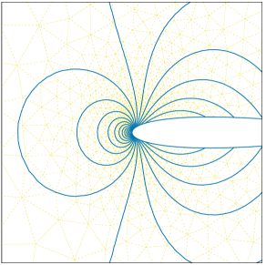
Figure 1: Subsonic inviscid flow around the NACA 0012 profile (${M_{\infty}}=0.5$, $\alpha=0\degree$): the computational mesh in the vicinity of the profile (left) and the isolines of the first component of ${\bm{w}_{h}}$ (right).

$z_{h}^{1}$                        $z_{h}^{2}$                        $z_{h}^{3}$                        $z_{h}^{4}$

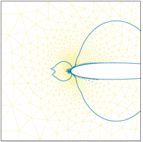
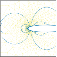
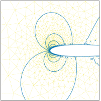
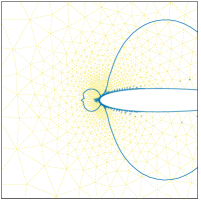
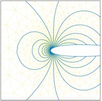
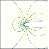
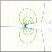
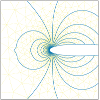
Figure 2: Subsonic inviscid flow around the NACA 0012 profile (${M_{\infty}}=0.5$, $\alpha=0\degree$), $J=$ drag coeff.: inconsistent (top) and consistent (bottom) discretization, the components of the discrete adjoint solutions ${\bm{z}_{h}}=(z_{h}^{1},z_{h}^{2},z_{h}^{3},z_{h}^{4})$ are shown.

7.2 Subsonic flows

In the following examples, we demonstrate the performance of the anisotropic mesh adaptive Algorithm 1, from Section 6.4, namely its $h$- and $hp$-variants.

7.2.1 Symmetric subsonic flow

We consider again the flow with ${M_{\infty}}=0.5$, $\alpha=0\degree$ and the target functional $J(\bm{w})$ is the drag coefficient according to (21). The exact value of the drag coefficient is $c_{D}=0$. Figure 3 shows the decrease of the error of the target quantity $J_{h}(\bm{w}_{h})-J(\bm{w})=J_{h}(\bm{w}_{h})$ and the corresponding estimates $\eta^{\rm I}$ and $\eta^{\rm I\!I}$ (cf. (96) and (102)) w. r. t. ${\mathrm{DoF}}$ for the $h$- (with $p=2$) and $hp$-version of the mesh adaptive algorithm. We observe that both $\eta^{\rm I}$ and $\eta^{\rm I\!I}$ approximate the true error quite accurately although $\eta^{\rm I}$ underestimates the error slightly. We see that the $hp$-version is superior to the $h$-version, as expected. Moreover, for the $hp$-variant, the error starts to stagnate at the level approximately 5E-07. We discuss this effect in Section 7.2.2, where it is better to observe.

Figure 4 shows the details of the $hp$-meshes of the anisotropic $hp$-adaptation after the 5th and 13th (the last) levels of adaptation. There is a strong $h$-refinement in the vicinity of the trailing edge due to the singularity, and outside of this small region, the strong $p$-adaptation is performed since the solution is sufficiently smooth.

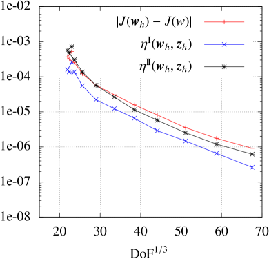
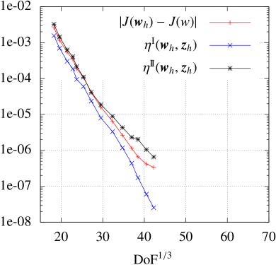
Figure 3: Subsonic inviscid flow around the NACA 0012 profile (${M_{\infty}}=0.5$, $\alpha=0\degree$), $J=$ drag coeff.: decrease of the error $J(\bm{w})-J({\bm{w}_{h}})$ and the goal-oriented error estimates $\eta^{\rm I}$ and $\eta^{\rm I\!I}$ with respect to the cube root of DOF for the $h$-refinement using $p=2$ DG approximations (left) and the $hp$-version (right).

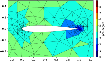
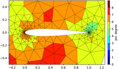
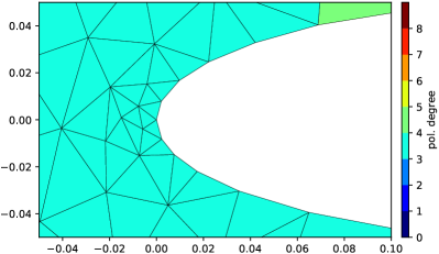
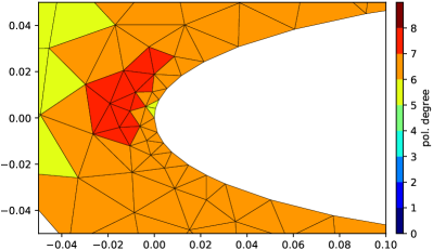
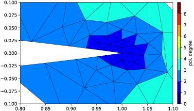
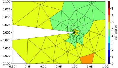
Figure 4: Subsonic inviscid flow around the NACA 0012 profile (${M_{\infty}}=0.5$, $\alpha=0\degree$), $J=$ drag coeff.: local polynomial degrees after the 5th (left) and 13th (right) levels of the anisotropic $hp$-mesh adaptation, the whole profile (top) and zooms of the leading (middle) and trailing (bottom) edge of the profile.

7.2.2 Non-symmetric subsonic flow

We consider the flow with ${M_{\infty}}=0.5$ and $\alpha=1.25\degree$ and the target functional is the drag as well as lift coefficients. Whereas the exact value of $c_{D}$ is again zero, the exact value of the lift coefficient has to be computed experimentally. We use the reference value of $c_{L}^{\mathrm{ref}}=1.757\cdot 10^{-1}\pm 10^{-4}$ achieved by the $hp$-adaptive algorithm.

Figure 5 shows the decrease of the error of the drag coefficient and their estimates w. r. t. ${\mathrm{DoF}}$. We observe that whereas both estimates are decreasing, the exact error stagnates at the level slightly below 1E-4. It means that the drag coefficient does not converge to the exact value $J(\bm{w})=0$ but to a positive value $c_{D}^{*}$. This effect was investigated in details in VassbergJameson_JA10 using several codes with a strong global refinement. Each of the tested code gave a small positive limit value $c_{D}^{*}$ (obtained by the Richardson extrapolation). Figure 5 shows also the quantity $|J(\bm{w}_{h})-c_{D}^{*}|$ with $c_{D}^{*}=6.8\cdot 10^{-5}$ which already converges as expected.

Furthermore, Figure 6 shows the decrease of the error of the lift coefficient and their estimates w. r. t. ${\mathrm{DoF}}$. We see that the error estimates work worse than in the previous case – $\eta^{\rm I}$ underestimates the error and, quite the other way, $\eta^{\rm I\!I}$ overestimates it almost ten times. This may be caused by the weaker regularity of the adjoint solution for the lift coefficient. In order to support this conjecture, we present Figure 7, which compares the first component of the adjoint solutions ${\bm{z}_{h}}$ and the corresponding $hp$-meshes for the drag coefficient and lift coefficients. These results indicate that

• the adjoint problem for the drag coefficient is quite smooth and then $p_{K}$ are high for $K$ in the surrounding of the profile ${\Gamma_{\mathrm{W}}}$,

• the adjoint problem for the lift coefficient has less regularity due to “boundary layers” along the profile and consequently, the strong $h$-refinement with low polynomial degree $p_{K}$ is presented for $K$ close to ${\Gamma_{\mathrm{W}}}$.

We remark that in the majority of articles on goal-oriented error estimates for the Euler equations, e.g., Hartmann2005Role ; Hartmann2006Derivation ; Hartmann2007Adjoint ; Hartmann2015Generalized , the numerical experiments are performed only for the drag coefficient. We have found only one experiment with the lift coefficient in Sharbatdar2018Mesh for the transonic flow around the NACA 0012 profile.

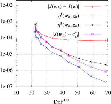
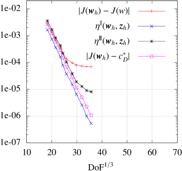
Figure 5: Subsonic inviscid flow around the NACA 0012 profile (${M_{\infty}}=0.5$, $\alpha=1.25\degree$), $J=$ drag coeff.: decrease of the error $J(\bm{w})-J({\bm{w}_{h}})$ and the goal-oriented error estimates $\eta^{\rm I}$ and $\eta^{\rm I\!I}$ with respect to the cube root of ${\mathrm{DoF}}$ the $h$-refinement using $p=2$ DG approximations (left) and the $hp$-version (right).

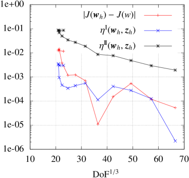
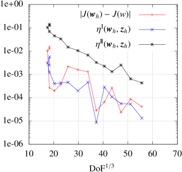
Figure 6: Subsonic inviscid flow around the NACA 0012 profile (${M_{\infty}}=0.5$, $\alpha=1.25\degree$), $J=$ lift coeff.: decrease of the error $J(\bm{w})-J({\bm{w}_{h}})$ and the goal-oriented error estimates $\eta^{\rm I}$ and $\eta^{\rm I\!I}$ with respect to the cube root of ${\mathrm{DoF}}$ the $h$-refinement using $p=2$ DG approximations (left) and the $hp$-version (right).

drag coefficient

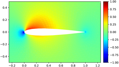
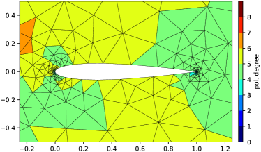
lift coefficient

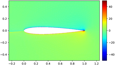
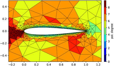
Figure 7: Subsonic inviscid flow around the NACA 0012 profile (${M_{\infty}}=0.5$, $\alpha=1.25\degree$): the first component of the discrete adjoint solution (left) on the final $hp-$mesh (right) for $J$ equal to the drag (top) and lift (bottom) coefficients.

7.3 Transonic flow

We consider the flow with ${M_{\infty}}=0.8$ and $\alpha=1.25\degree$ which leads to two shock waves. We apply the shock-capturing technique based on the artificial viscosity whose amount is given by the jump indicator, see (DGM-book, , Section 8.5) or feikuc2007 . The target functional $J$ is both drag and lift coefficients, the reference values $c_{D}^{\mathrm{ref}}=2.135\times 10^{-2}$ and $c_{L}^{\mathrm{ref}}=3.33\times 10^{-1}$ were computed by the $hp$-anisotropic adaptation method.

Figure 8 shows the decrease of the error of the target quantity and the error estimates $\eta^{\rm I}$ and $\eta^{\rm I\!I}$ w. r. t. ${\mathrm{DoF}}$. For both target functionals, $\eta^{\rm I}$ underestimates and $\eta^{\rm I\!I}$ overestimates the true error by a factor at most $10$. We suppose that such overestimation is caused by the high-order reconstruction from Section 6.2, which is not sufficiently accurate for problems having discontinuous solution. Moreover, Figure 9 shows the final $hp$-grids and the corresponding distribution of the Mach number and the first component of the adjoint solution. A strong $h$-refinement with low polynomial approximation degrees along both shock waves is observed. A sharp capturing of both waves are easily to see.

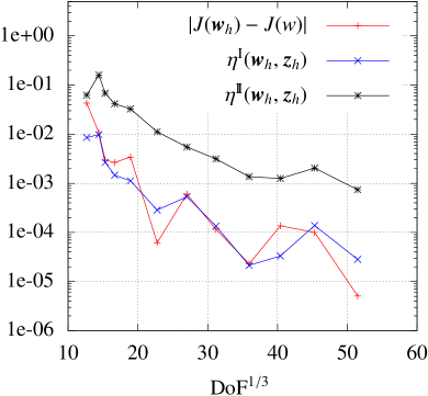
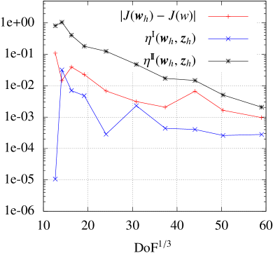
Figure 8: Transonic inviscid flow around the NACA 0012 profile (${M_{\infty}}=0.8$, $\alpha=1.25\degree$): decrease of the error $J(\bm{w})-J({\bm{w}_{h}})$ and the goal-oriented error estimates $\eta^{\rm I}$ and $\eta^{\rm I\!I}$ for $J$ equal to the drag (left) and lift (right) coefficients w.r.t. the cube root of DOF.

$J(u)$=drag coefficient                            $J(u)$=lift coefficient

$hp$-mesh

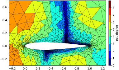
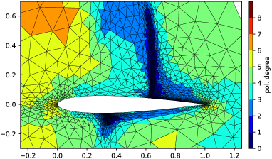
Mach number

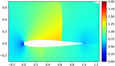
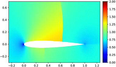
first component of ${\bm{z}_{h}}$

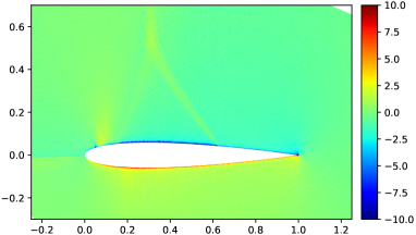
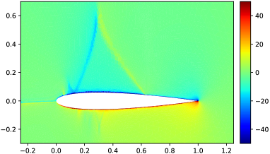
Figure 9: Transonic inviscid flow around the NACA 0012 profile (${M_{\infty}}=0.8$, $\alpha=1.25\degree$): $J$ equal to the drag (left) and lift (right) coefficients using the $hp$-anisotropic refinement.

8 Conclusion

We presented the goal-oriented adaptive discontinuous Galerkin method for the numerical solution of the Euler equations. The DG discretization leads to the system of nonlinear algebraic equations which are solved iteratively by an iterative solver based on a suitable linearization of the numerical scheme. This linearization is employed for the definition of the adjoint problem. The careful treatment of the impermeable wall condition and the modification of target functional admit the adjoint consistent discretization, which was proved analytically and supported by numerical experiments. Therefore, iterative solvers not-based on the proper differentiation can be used in the goal-oriented computations.

Furthermore, we extended the goal-oriented anisotropic $hp$-mesh adaptive technique from DWR_AMA ; ESCO-18 to the Euler equations. We presented numerical examples of subsonic as well as transonic flows demonstrating the computational performance of this adaptive method. Although we observed the exponential convergence of the error only for some numerical examples, the potential of the $hp$-adaptive technique is obvious.

Conflict of interest

The authors declare that they have no conflict of interest.

References

• (1) Balan, A., Woopen, M., May, G.: Adjoint-based $hp$-adaptivity on anisotropic meshes for high-order compressible flow simulations. Comput. Fluids 139, 47 – 67 (2016)
• (2) Bangerth, W., Rannacher, R.: Adaptive Finite Element Methods for Differential Equations. Lectures in Mathematics. ETH Zürich. Birkhäuser Verlag (2003)
• (3) Bartoš, O., Dolejší, V., May, G., , Rangarajan, A., Roskovec, F.: Goal-oriented anisotropic $hp$-mesh optimization technique for linear convection-diffusion-reaction problem. Comput. Math. Appl. 78(9), 2973–2993 (2019)
• (4) Bassi, F., Rebay, S.: High-order accurate discontinuous finite element solution of the 2D Euler equations. J. Comput. Phys. 138, 251–285 (1997)
• (5) Bassi, F., Rebay, S.: Numerical evaluation of two discontinuous Galerkin methods for the compressible Navier–Stokes equations. Int. J. Numer. Methods Fluids 40, 197–207 (2002)
• (6) Becker, R., Rannacher, R.: An optimal control approach to a-posteriori error estimation in finite element methods. Acta Numerica 10, 1–102 (2001)
• (7) Ceze, M., Fidkowski, K.J.: Anisotropic $hp$-adaptation framework for functional prediction. AIAA Journal 51(2), 492–509 (2012)
• (8) Dolejší, V.: A design of residual error estimates for a high order BDF-DGFE method applied to compressible flows. Int. J. Numer. Methods Fluids 73(6), 523–559 (2013)
• (9) Dolejší, V., Feistauer, M.: Semi-implicit discontinuous Galerkin finite element method for the numerical solution of inviscid compressible flow. J. Comput. Phys. 198(2), 727–746 (2004)
• (10) Dolejší, V., Feistauer, M.: Discontinuous Galerkin Method – Analysis and Applications to Compressible Flow. Springer Series in Computational Mathematics 48. Springer, Cham (2015)
• (11) Dolejší, V., May, G., Rangarajan, A., Roskovec, F.: A goal-oriented high-order anisotropic mesh adaptation using discontinuous Galerkin method for linear convection-diffusion-reaction problems. SIAM Journal on Scientific Computing 41(3), A1899–A1922 (2019)
• (12) Dolejší, V., Roskovec, F., Vlasák, M.: Residual based error estimates for the space-time discontinuous Galerkin method applied to the compressible flows. Comput. Fluids 117, 304–324 (2015)
• (13) Feistauer, M., Felcman, J., Straškraba, I.: Mathematical and Computational Methods for Compressible Flow. Clarendon Press, Oxford (2003)
• (14) Feistauer, M., Kučera, V.: On a robust discontinuous Galerkin technique for the solution of compressible flow. J. Comput. Phys. 224, 208–221 (2007)
• (15) Fidkowski, K., Darmofal, D.: Review of output-based error estimation and mesh adaptation in computational fluid dynamics. AIAA Journal 49(4), 673–694 (2011)
• (16) Fidkowski, K.J., Luo, Y.: Output-based space-time mesh adaptation for the compressible Navier-Stokes equations. J. Comput. Phys. 230(14), 5753–5773 (2011)
• (17) Giles, M., Pierce, N.: Adjoint equations in CFD - Duality, boundary conditions and solution behaviour. In: 13th Computational Fluid Dynamics Conference. American Institute of Aeronautics and Astronautics (1997)
• (18) Giles, M., Süli, E.: Adjoint methods for PDEs: a posteriori error analysis and postprocessing by duality. Acta Numerica 11, 145–236 (2002)
• (19) Harriman, K., Gavaghan, D.J., Suli, E.: The importance of adjoint consistency in the approximation of linear functionals using the discontinuous Galerkin finite element method. Tech. rep., Oxford University Computing Laboratory (2004)
• (20) Hartmann, R.: The Role of the Jacobian in the Adaptive Discontinuous Galerkin Method for the Compressible Euler Equations. Springer Berlin Heidelberg, Berlin, Heidelberg (2005)
• (21) Hartmann, R.: Derivation of an adjoint consistent discontinuous Galerkin discretization of the compressible Euler equations. In: G. Lube, G. Papin (Eds): International Conference on Boundary and Interior layers (2006)
• (22) Hartmann, R.: Adjoint Consistency Analysis of Discontinuous Galerkin Discretizations. SIAM J. Numer. Anal. 45(6), 2671–2696 (2007)
• (23) Hartmann, R., Houston, P.: Adaptive discontinuous Galerkin finite element methods for the compressible Euler equations. J. Comput. Phys. 183(2), 508–532 (2002)
• (24) Hartmann, R., Houston, P.: Symmetric interior penalty DG methods for the compressible Navier-Stokes equations I: Method formulation. Int. J. Numer. Anal. Model. 1, 1–20 (2006)
• (25) Hartmann, R., Houston, P.: Symmetric interior penalty DG methods for the compressible Navier-Stokes equations II: Goal-oriented a posteriori error estimation. Int. J. Numer. Anal. Model. 3, 141–162 (2006)
• (26) Hartmann, R., Leicht, T.: Generalized adjoint consistent treatment of wall boundary conditions for compressible flows. Journal of Computational Physics 300, 754–778 (2015)
• (27) Leicht, T., Hartmann, R.: Anisotropic mesh refinement for discontinuous Galerkin methods in two-dimensional aerodynamic flow simulations. Int. J. Numer. Methods Fluids 56(11), 2111–2138 (2008)
• (28) Loseille, A., Dervieux, A., Alauzet, F.: Fully anisotropic goal-oriented mesh adaptation for 3D steady Euler equations. J. Comput. Phys. 229(8), 2866–2897 (2010)
• (29) Lu, J.: An a posteriori control framework for adaptive precision optimization using discontinuous galerkin finite element method. Ph.D. thesis, M.I.T. (2005)
• (30) Rangarajan, A., May, G., Dolejsi, V.: Adjoint-based anisotropic $hp$-adaptation for discontinuous galerkin methods using a continuous mesh model. Journal of Computational Physics 409, 109321 (2020)
• (31) Sharbatdar, M., Ollivier-Gooch, C.: Mesh adaptation using ${C}^{1}$ interpolation of the solution in an unstructured finite volume solver. International Journal for Numerical Methods in Fluids 86(10), 637–654 (2018)
• (32) Vassberg, J.C., Jameson, A.: In pursuit of grid convergence for two-dimensional euler solutions. Journal of Aircraft 47(4), 1152–1166 (2010)
• (33) Venditti, D., Darmofal, D.: Grid adaptation for functional outputs: Application to two-dimensional inviscid flows. J. Comput. Phys. 176(1), 40–69 (2002)
• (34) Venditti, D., Darmofal, D.: Anisotropic grid adaptation for functional outputs: Application to two-dimensional viscous flows. J. Comput. Phys. 187(1), 22–46 (2003)
• (35) Vijayasundaram, G.: Transonic flow simulation using upstream centered scheme of Godunov type in finite elements. J. Comput. Phys. 63, 416–433 (1986)
• (36) Yano, M., Darmofal, D.L.: An optimization-based framework for anisotropic simplex mesh adaptation. J. Comput. Phys. 231(22), 7626–7649 (2012)