Programming by Rewards

Abstract.

We formalize and study “programming by rewards” (PBR), a new approach for specifying and synthesizing subroutines for optimizing some quantitative metric such as performance, resource utilization, or correctness over a benchmark. A PBR specification consists of (1) input features $\mathbf{x}$, and (2) a reward function $r$, modeled as a black-box component (which we can only run), that assigns a reward for each execution. The goal of the synthesizer is to synthesize a decision function $f$ which transforms the features to a decision value for the black-box component so as to maximize the expected reward $E[r\circ f(\mathbf{x})]$ for executing decisions $f(\mathbf{x})$ for various values of $\mathbf{x}$.

We consider a space of decision functions in a DSL of loop-free if-then-else programs, which can branch on linear functions of the input features in a tree-structure and compute a linear function of the inputs in the leaves of the tree. We find that this DSL captures decision functions that are manually written in practice by programmers. Our technical contribution is the use of continuous-optimization techniques to perform synthesis of such decision functions as if-then-else programs. We also show that the framework is theoretically-founded —in cases when the rewards satisfy nice properties, the synthesized code is optimal in a precise sense.

PBR hits a sweet-spot between program synthesis techniques that require the entire system $r\circ f$ as a white-box, and reinforcement learning (RL) techniques that treat the entire system $r\circ f$ as a black-box. PBR takes a middle path treating $f$ as a white-box, thereby exploiting the structure of $f$ to get better accuracy and faster convergence, and treating $r$ as a black-box, thereby scaling to large real-world systems. Our algorithms are provably more accurate and sample efficient than existing synthesis-based and reinforcement learning-based techniques under certain assumptions.

We have leveraged PBR to synthesize non-trivial decision functions related to search and ranking heuristics in the PROSE codebase (an industrial strength program synthesis framework) and achieve competitive results to manually written procedures over multiple man years of tuning. We present empirical evaluation against other baseline techniques over real-world case studies (including PROSE) as well on simple synthetic benchmarks.

1. Introduction

Consider the following scenario, which routinely arises while writing software. A developer wants to write a sub-routine to decide how to set some threshold parameter, such as timeout value, before executing a software component (say a database system or a networking system). First, they may not apriori know what the threshold needs to be for a particular input — because fundamentally there may not be any ”right” threshold for a given input, but it may depend on the myriad program variables in complex ways that eventually affects the execution of the software. Suppose the developer makes a decision to set the threshold to some value $\tau$. After the component finishes executing, the developer may be able to measure some non-functional metric such as latency or throughput or resource utilization to get feedback on whether the threshold $\tau$ was a ”good” or ”bad” choice. Such feedback can be given as a ”reward” (using the terminology of reinforcement learning) to improve future choices for the threshold $\tau$.

The performance and functionality of large scale software is dependent on many such thresholds, which we call as decision values or more succinctly, decisions. Typically, decisions are tuned to suitable values depending on the variables that represent the state of the program (such as size of internal queues) as well as the state of the environment (such as number of requests received per second), and the number of such dependencies can be very large, or ”high-dimensional”, to use terminology of machine learning. Often, such decisions are set in the code, using custom logic, as shown in the example code in Figure 1. We call functions with such custom logic as decision functions. Decision functions also generalize configuration files (see Figure 1 (left)), which is often part of large code-bases. Each line in the configuration file can be thought of as trivial decision functions that return constant values as decisions.

We propose a new framework, Programming by Rewards, abbreviated as PBR, for automatically synthesizing and tuning decision functions in standard settings. A PBR specification consists of

1. The input features $x$, with their data types, and the decision type. For example, in Figure 1, for the decision function ScoreLinesMap the input features are selection and lines, both having type double, and the decision type is also double, which is the return type of the method.

2. A reward function $r$, modeled as a black-box component, that consumes the output of the decision function, executes an arbitrarily complicated software module, and assigns a reward value for the execution of the black-box software module with the provided decision value. For example, in Figure 1, the black-box is the PROSE engine (PROSE, 2015) which takes the return values of ScoreLinesMap and other such decision functions as decision values, and executes a complicated program synthesis engine, and assigns a reward like total execution time or accuracy of the synthesized program. Other examples of black-box engines could be communications software such as Skype or Zoom, or database engines such as SQLServer, where the reward value can be proportional to latency seen by the end-user or a combination of total execution time.

The framework relies on suitable programmer-defined rewards that indicate how well the decision value returned by the decision function eventually affects the success of the overarching software itself, represented by the the reward function $r$. We formalize the problem of synthesizing decision functions given only execution (or invocation) access to the reward function $r$. Furthermore, in practice, due to changes in the environment (such as load on the system), two invocations of the black-box with the same decision value can result in different reward values. Hence, $r$ need not be deterministic. We optimize the expected value of the reward (see Definition 3 in Section 2), while allowing for randomness inside the reward function.

Prior work in this area follows one of the three approaches:

1. In the rule-based approach, which is widely used by practitioners, the programmer writes decision functions using custom code, which has domain-specific logic to compute decision values in terms of input features. For example, the decision function  ScoreLinesMap shown in Figure 1 uses three manually chosen parameter values minscore,alpha and beta, to compute one decision value as a function of the input features sel and lines, which is returned by the function. The programmer can tweak the custom code based on a few observed rewards, but in general, setting a larger number of parameters manually can lead to significantly sub-optimal rewards. Further, the decision function  ScoreLinesMap and the parameter values do not adapt automatically as the environment of the software changes, which is undesirable.

2. In the sketch-based synthesis approach, the idea is to specify the decision function as a template with “holes”. For example, in the decision function ScoreLinesMap shown in Figure 1, the programmer can leave the values of the parameters minScore, alpha and beta as holes and leave it to the synthesis engine to synthesize values for these holes such that a quantitative specification that optimizes the reward value is satisfied. Though Sketching has been primarily used with correctness specifications (which are Boolean) (Bodik and Solar-Lezama, 2006), prior work has explored sketching to optimize quantitative specifications such as reward values (Chaudhuri et al., 2014). In this setting, the entire software $r\circ f$ is required to be white-box for program synthesis to work, which makes the approach challenging to scale.

3. In the reinforcement learning approach, the decision function is learned automatically using an ML formulation, which is trained from traces of executions of the code so as to optimize the expected value of the rewards (Agarwal et al., 2016; Sutton and Barto, 2011). This approach has attracted much attention recently due to increasing popularity of machine learning. In this setting, the entire software $r\circ f$ is treated as a black-box, and the algorithms to learn $f$ need a large number of samples to learn when the number of features and parameters are large.

PBR hits a sweet-spot between program synthesis and reinforcement learning approaches mentioned above. PBR takes a middle path, treating the decision code $f$ as a white-box, thereby exploiting the structure of $f$ to get better accuracy and faster convergence, and treating $r$ as a black-box, thereby scaling to real-world systems. We consider a space of decision functions in a DSL of loop-free if-then-else programs, which can branch on the input features in a tree-structure and compute a linear function of the inputs in the leaves of the tree. We find that this DSL captures decision functions that are manually written in practice by programmers.

Our methods work in both the offline and online settings. In the offline setting we have access to all the executions and reward values apriori. In the online setting, a reward is assigned online in response to a decision value, and PBR uses the reward to improve the decision function. In practical large-scale systems, online setting is more practical and general, so we mostly focus on this setting from algorithm development viewpoint. Our most substantial case study (Section  5.2) is also in the context of black-box reward functions in an online setting. However, we also compare with baselines (especially based on sketch-based synthesis methods) having offline access all the data, and having white-box access to the reward functions (Section  5.3).

Our key technical contribution is the use of continuous-optimization techniques, specifically gradient descent, to perform synthesis of decision functions such as if-then-else programs, with small update and sample complexity, i.e., the execution time as well as the number of black-box reward executions required by our techniques are relatively small. However, there are several challenges in applying gradient descent techniques in PBR setting. First, we only have restricted access to the reward function $r$ so computing gradient itself is challenging. Furthermore, the general decision tree functions are non-smooth, piece-wise linear functions which are challenging to capture with continuous optimization methods.

In this work, we make two-fold contributions on this front. First, we build upon well-established approach in the optimization literature, that gradient based methods allow inexact, noisy but unbiased gradient estimates, which can be obtained by invoking reward function $r$ on random perturbation of decision values. However, such methods can lead to large sample complexity (i.e. number of executions of $r$) if we have a large number of parameters. If the decision function is a linear function or if it is an if-then-else program with small number of decision values, then we can provide significantly more efficient gradient estimation methods. Formally, let $d$ be the number of parameters in the system, and let $m$ be the number of decisions made in the system. Our core result is that we can automatically synthesize decision functions if they are loop-free and use linear operators. Specifically, even though there may be many parameters in the system ($d\gg m$), we design ML algorithms with complexity proportional to $m$ rather than $d$. Since $m$ is typically much smaller than $d$, our approach has significant advantages over existing approaches, whose complexity scales with $d$. As an example, the decision function ScoreLinesMap (in Figure 1) is a linear model with $m=1$ and $d=3$. The decision function IsLikelyDataRatio (in Figure 1) can be encoded as a decision tree model with (on the order of) 10 parameters representing the weights and predicates in a shallow tree. In this case, we have a decision tree with $d\sim 10$ and $m=1$. In this work, we propose novel ML algorithms whose complexity depends on $m$ rather than $d$ for linear models and decision trees. Furthermore, for certain cases, we provide rigorous bounds on the efficiency of the proposed methods.

Second, we show how decision trees can be modeled using a continuous shallow network model under structural constraints, which enables usage of standard gradient descent type of methods for learning the parameters of decision trees with only black-box reward $r$ (see Section 4.3).

Finally, we conduct extensive experiments to validate that our PBR based methods can indeed be used to efficiently synthesize programs in real-world codebases using only black-box reward function (Section 5.2). In particular, for $\mathsf{PROSE}$ (PROSE, 2015), which is a complicated system with nearly 70 ranking related heuristics fine-tuned over several years, our method can synthesize all the heuristics while achieving competitive accuracy to hand-tuned systems, after training for a few days and after only about 250 calls to the reward function; in $\mathsf{PROSE}$ each reward function call requires synthesizing programs for about $740$ benchmarks and then computing their accuracy, thus highlighting the need to optimize sample complexity of PBR methods. Furthermore, we show that standard reinforcement style learning methods when used in completely black-box manner indeed suffer from poorer sample complexity in such problems (Section 5.4). Finally, we observe that even when we provide existing sketch based methods–either using CEGIS (Counterexample Based Inductive Synthesis) on top of SAT (Bodik and Solar-Lezama, 2006) or numerical methods (Chaudhuri et al., 2014)–with whitebox access to the entire reward function and also provide apriori access to all the execution traces (i.e. offline data), their computational and sample complexity is significantly higher than our techniques (Section 5.3).

In summary, the paper makes the following contributions:

1. We observe Imp (Definition 1) to be rich language that accurately models typical decision functions in practice and also identify some important sub-classes of Imp.

2. We formalize Programming by Rewards (PBR) with Imp DSL and also present an equivalent formalism as that of learning decision trees with black-box rewards.

3. We present novel algorithms for learning decision tree as well as linear models with rewards and provide rigorous guarantees for the latter.

4. We present strong empirical validation of our approach on an industrial strength codebase, demonstrating both sample and computational efficiency.

Paper Organization: Section 2 formally specifies the PBR problem, provides the DSL that we consider and motivates it using existing work and inspection of a few real-world codebases. Then in Section 3, we provide overview of how we set up the problem as a decision-tree learning problem and set up the key metrics to be considered while designing the algorithms. In Section 4 we provide specific PBR algorithms for three different DSLs and in certain cases, provide rigorous guarantees. In Section 5 we provide empirical evaluation of our method and compare it against relevant sketching and reinforcement learning based baselines. In Section 6, we survey related work, and finally conclude with Section 7.

⬇

[Resource1]

RefreshInterval=00:01:00

PriorityHighUnderloaded=97

PriorityHighOverloaded=98

PriorityLowUnderloaded=88

PriorityLowOverloaded=90

...

[Resource2]

RefreshInterval=00:01:00

PriorityHighUnderloaded=80

PriorityHighOverloaded=90

...

⬇

double ScoreLinesMap(double sel, double lines) {

double minScore = 100.0;

double alpha = 1.0; double beta = 1.0;

return alpha * sel + beta * lines + minScore * 20;

}

bool IsLikelyDataRatio(int dataCount, int totalCount) {

if (totalCount < 10) return dataCount >= 6;

if (totalCount < 20) return dataCount >= 15;

if (totalCount < 50) return dataCount >= 30;

return dataCount / (double) totalCount >= 0.6;

}

Figure 1. (left) A configuration file is a common coding pattern for hard-coding constants/settings in software, and (right) Implementations of a rule for scoring programs, and a control logic for determining the value of a boolean state variable; both part of the widely-deployed program synthesis SDK, $\mathsf{PROSE}$ (PROSE, 2015).

2. Problem Formulation

This section formally introduces Programming by Rewards (PBR) problem for synthesizing decision functions. We start by motivating and defining the class of decision functions considered in this work. We set up the PBR problem with an example, and discuss how it relates to the standard sketch-based synthesis problem. Next, we give an equivalent formulation of the problem using decision trees. This lets us formulate the problem as a learning problem which can leverage continuous-optimization based techniques and provide significantly more efficient algorithms.

2.1. Decision functions in real-world software

We motivate our approach by showing various examples of decision functions that are currently written manually by programmers. We performed extensive studies of such decision functions in two domains:

• Efficient search. There are many problem domains where we need to search through the space of solutions in a combinatorial space. This includes SAT and SMT solvers, as well as program verification and synthesis engines. Software written for such domains often involve several heuristic decisions made in the code. Figure 2 shows a snippet of a hybrid branching heuristic implemented in the MapleGlucose SAT solver (Liang et al., 2016). We notice the rather obscure choice of constants and thresholds in the conditionals as part of the heuristic.

  ⬇

  bool Solver::search(int nof_conflicts)

  {

  ...

  for (;;) {

  ...

  if (S > 0.06)

  S -= 0.000001;

  if(conflicts % 5000 == 0 && var_decay < 0.95)

  var_decay += 0.01;

  ...

  }

  }

  Figure 2. Code snippet from MapleGlucose SAT solver (Liang et al., 2016) that implements a hybrid LRB-VSIDS branching heuristic in the search procedure.

• Ranking heuristics. Program synthesis and in particular programming-by-example engines, e.g., PROSE (which has found adoption in multiple mass-market products), need to deal with ambiguity in the user’s intent expressed using a few input-output examples. This is done by carefully implementing ranking heuristics to select an intended program from among the many that satisfy the few input-output examples provided by the user. A significant fraction of developer time is spent on hand-crafting these heuristics for each new domain where PROSE is applied. Each new domain is characterized by a different DSL, and the nature of the DSL and the programs we seek determines which production rules we want to favor, which is in turn determined by the decision functions. We study decision functions from PROSE, which is an industrial strength program synthesis system. The example decision functions in Figure 1 is from real-world ingestion software built on top of PROSE. The function implements a heuristic for deciding header to data ratio in the input file; the examples in Figures 6 and 15 are ranking heuristics for example-based string transformations widely used inside a mass-market spreadsheet product. We observe that these decision functions either involve simple (linear) operations on the input variables, or compute decisions based simple branching decisions on the input variables.

• Real-time services. Large-scale services for workload management and scheduling, cloud database management servers (AzureSQL), etc. often have configuration settings and parameters to ensure optimal performance of the service in terms of latency, efficiency and cost. Often, these settings are defined in one-size-fits-all manner relying on wisdom-of-the-crowd or other heuristics. Figure 1 (left) shows the configuration snippet from a real-time scheduling service that is part of a mass-market commercial software system. These are the simplest type of decision functions, i.e. constants that one need to set optimally in a dynamic fashion to account for the continuously-changing system.

We observe that the decision function instances cited above, and more generally arising in these software domains, have the following characteristics:

1. Operations are restricted to linear combinations of program variables; however, the parameters in the operation can be real numbers (expressed using floating point or decimal notation).

2. There are nested if-then-else conditions, but the conditions are also expressible by linear combinations of input variables.

3. There are no loops.

This observation lets us define the following language that contains commonly-arising decision functions. Variants of this language have been used in program synthesis and in sketching (Chaudhuri et al., 2014; Bornholt et al., 2016).

2.2. A DSL for decision functions

Definition 1 (Language Imp).

We consider the language Imp of programs with imperative updates and if-then-else statements without loops. Programs in Imp operate over real valued variables; in particular, Imp allows linear transformations over the input variables $x\in\mathbb{R}$ in both conditionals as well as assignments to local variables $o\in\mathbb{R}$. The function returns a tuple of local variables as decision values.

$$P ::= S;\textbf{{return}}\ (o_{1},o_{2},\ldots,o_{m})$$

$$S ::= o=E$$

$$\big{|}~{}\textbf{{if}}~{}(E>0)~{}\textbf{{then}}~{}S_{1}~{}\textbf{{else}}~{}S_{2}$$

$$\big{|}~{}S_{1};S_{2}$$

$$E ::= W_{1}\cdot x_{1}+W_{2}\cdot x_{2}+\cdots+W_{p}\cdot x_{p}+W_{p+1}$$

$$W ::= \mathbf{K}~{}\big{|}~{}??$$

where $\mathbf{K}$ is a numerical constant in $\mathbb{R}$, and ”??” denotes a hole.

Given the definition above, we can define decision functions formally as programs in Imp  that take $p$ program variables as input and return $m$ decision values as output. It is easy to see that the functions in Figure 1 are in Imp, with $p=2$ and $m=1$. Furthermore, we observe that in some of the real-world settings, the decision functions that programmers write (including some of the aforementioned examples) do not require the full expressiveness of Imp, but can be even more concisely specified (as presented below) — this facilitates provably-efficient algorithms in such settings (Section 4).

Definition 2 (Languages Linear and Const).

1. $\textsc{Linear}\subset\textsc{Imp}$ consists of linear functions with no if-then-else branches; e.g. Figure 1 (right), Figures 6 and 15.
2. $\textsc{Const}\subset\textsc{Linear}$ consists of constants, the most basic form of decisions, $W_{1}=W_{2}=\dots=W_{p}=0$ in Linear; e.g. Figure 1 (left).

2.3. PBR formulation

Let $f\in\textsc{Imp}$ denote a decision function. In our PBR setup, the decision given by $f$ is fed into a black-box program (software) in some arbitrary language $\mathcal{L}$ (typically much more complex than Imp); we have no knowledge of $\mathcal{L}$. Let us denote by $r$, a reward metric that quantifies some aspect of executing the software using the decisions given by $f$. The reward may be assigned a value, which depends not only on correctness of the execution but also on nonfunctional aspects such as performance, latency, throughput of resource utilization. Formally, $r:f\mapsto\mathbb{R}$. The following example illustrates this set up.

Example 0.

⬇

int ParseAndProcessFile(string fileName)

{

string contents = read(fileName);

int[2] counts = getCounts(contents);

if (PBR.DecisionFunction(PBRID_IsLikelyDataRatio, count[0], count[1]))

preProcess(fileName);

parseFile(FileName);

return (processFile(fileName));

}

void main()

{

double successes = 0.0;

StopWatch sw = new StopWatch();

sw.Start();

foreach (string fileName in Config.Benchmarks):

successes += ParseAndProcessFile(fileName) > 0 ? 1: 0;

sw.Stop();

double reward = (success/Config.Benchmarks.Length) - (sw.ElapsedMilliseconds/1000);

PBR.AssignReward(reward);

}

Figure 3. A C# program that uses the PBR system to automatically learn a decision function in the place of the manually written function IsLikelyDataRatio from Figure 1.

Consider the program shown in Figure 3. Here, we show how to use the PBR system to automatically learn a decision function in place of the manually written function IsLikelyDataRatio from Figure 1. The decision function learned by the PBR system is identified by a unique identifier PBRID_IsLikelyDataRatio for the function in the PBR.DecisionFunction method. For each file, the function determines if we need to invoke an expensive pre-processing method before parsing the file. A reward metric for the execution, which could potentially have multiple invocations of many decision functions, is assigned using the PBR.AssignReward method.

In this example, we have a single instance of a decision function invoked multiple times, once for each file. The reward takes into account both the effectiveness of processing, which is the number of files processed successfully, and the efficiency of processing as measured by the time taken for processing all the files. Ideally, we want to balance the goals of successfully processing the files with spending less time on pre-processing. The goal of the PBR system is to learn a decision function which maximizes the expected reward.

With this notation, we formally state the Programming By Rewards (PBR) problem.

Definition 3 (Programming By Rewards (PBR)).

Given a specification consisting of:

1. The input variables $\mathbf{x}\in\mathbb{R}^{p}$ to the decision function $f:\mathbb{R}^{p}\to\mathbb{R}^{m}$, with their data types, and the decision type,

2. Query-access to a black-box reward function $r:\mathbb{R}^{m}\to\mathbb{R}$, which assigns a reward value for the execution of the software with the provided decision values of $f$,

the goal of PBR is to synthesize an optimal $f\in\emph{{Imp}}$ such that:

$$f\in\arg\max_{f\in\emph{{Imp}}}~{}~{}\mathbb{E}[r(f)],$$

where $\mathbb{E}$ denotes the expectation with respect to the randomness in $r$.

That is, the programmer provides input variables and reward function $r$, and expects a PBR system to synthesize the program from the Implanguage (or a subset of Impdiscussed in next section). Note that, our methods allow programmers to provide a sketch of the program from Imp, and in general, that would lead to more efficiency. But as not providing any sketch is the extreme version of this problem, we focus on it from our algorithmic development point of view, and leave further experiments on completing partial sketches via rewards for future work.

We remark that the black-box reward functions $r$ can be expensive to execute (or even disruptive, in settings where the learning needs to happen in an online fashion in real-world deployments). Hence, the complexity of any algorithm to the PBR problem needs to be stated in terms of the total number of queries made to the reward function to learn a ”sufficiently good” solution—we refer to this as the sample complexity.

The PBR problem can, in principle, be phrased as a program synthesis problem with the language Imp being used to specify a sketch representing the space of programs we need to search for synthesizing decision functions. However, such an approach runs into many difficulties. The parameters we want to determine range over real values, which do not work well with enumerative search or symbolic methods using SMT solvers. Further, the outputs of decision functions routinely feed into modules with millions of lines of code. The reward function $r$ can be quantitative and the reward values can arrive much later in execution after many large modules are executed with the decision values. Consequently, if we want to model PBR using sketching, the whole program (which includes methods such as preProcess and parseFile in the example above) need to be modeled as a white-box. Moreover, it is unclear as to how concepts such as execution time can be modeled using sketching.

Aforementioned aspects distinguish our problem formulation from the standard sketch-based synthesis formulations. In particular, sketching techniques that take in boolean (Bodik and Solar-Lezama, 2006) or quantitative specification (Chaudhuri et al., 2014), require complete knowledge of the program that contains the holes, and white-box access to some functional form of the reward function (which also needs to satisfy some constraints, and can not be arbitrary). Consequently, many practical instances of PBR can not be posed as sketches.

3. Equivalence to Decision Tree Learning

We observe that the IMP programs are a form of decision trees with linear comparisons in nodes and linear computations in leaves. Below, we establish the PBR learning problem as that of learning optimal decision trees in presence of a black-box reward function, and then describe algorithms for the latter. This allows us to make use of an elegant notation for describing our algorithms as well as makes our algorithms relevant to a broader community.

For ease of exposition, we will consider $m=1$ case below (i.e. the decision function returns only one value); it is straight-forward to extend to the general setting.

Definition 4 (Decision Trees).

A binary decision tree of height $h$ represents a piece-wise linear function $f_{T}(\mathbf{x};\mathbf{W},\bm{\Theta}):\mathbb{R}^{p}\to\mathbb{R}$ parameterized by (a) weights $\mathbf{W}=\{\mathbf{w}_{ij}\in\mathbb{R}^{p},b_{ij}\in\mathbb{R}\}$, with $\mathbf{w}_{ij}$ at $(i,j)$th node ($j$th node at depth $i$) computing decisions of the form $\langle\mathbf{w}_{ij},\mathbf{x}\rangle+b_{ij}>0$, and (b) $\bm{\Theta}=\{\bm{\theta}_{j}\in\mathbb{R}^{p}\}$, with parameters $\bm{\theta}_{j}\in\mathbb{R}^{p}$ that encode a linear model at each leaf node. The computational semantics of the function $f_{T}$ is as follows: An input $\mathbf{x}\in\mathbb{R}^{p}$ traverses a unique root-to-leaf path in the tree, based on the results of the binary decisions at each height, with the convention that the left branch is taken if the decision at the node is satisfied, or the right branch otherwise. The output of the decision tree is $\bm{\theta}_{*}\cdot\mathbf{x}$, where $*$ is the leaf node reached by $\mathbf{x}$ and $\cdot$ denotes the dot product.

Remark 1.

The standard ”regression tree” (decision tree for real-valued predictions) of height $h$ is a piece-wise constant function, i.e., $f_{T}$ realizes at most $2^{h}$ unique values (one per leaf node). We consider a more general and expressive tree, that represents a piece-wise linear function, as defined above.

Remark 2.

The above definition of decision tree can be extended to the general $m$ setting, by allowing the leaf node parameters to be $\bm{\theta}_{j}\in\mathbb{R}^{m\times p}$; $\mathbf{W}$ remains the same as above.

⬇

double throttle(double latency, double load, double min)

{

double rate = 1.0;

if (latency < 5) return load;

if (load > 100)

rate = 0.5;

if (load * rate < min) return min;

return load * rate;

}

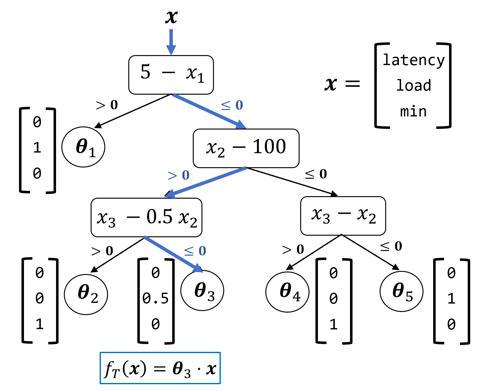
Figure 4. (left) Example decision function in Imp, and (right) its equivalent binary decision tree with linear models in the leaf nodes.

Figure 4 illustrates such a decision tree of height 3 computing a decision function. We note the computational semantics of a decision tree is identical to that of if-then-else programs in Imp. Below, we make this observation precise.

Lemma 1.

For every program $f\in\emph{{Imp}}$ defined over $p$ variables, there is a decision tree $f_{T}$, as given in Definition 4 that behaves identical to $f$ on every input $\mathbf{x}\in\mathbb{R}^{p}$. In other words, for every $f\in\emph{{Imp}}$, there is $f_{T}$ such that $f=f_{T}$.

In the worst case, a sequence of $h$ conditionals in Imp can result in a complete tree of depth $h$ and size $2^{h}$. However, in practice, we find that our algorithms tend to learn sparse (i.e. with many empty nodes that can be pruned) trees. Also, the sample complexity of our algorithms depend only on $m$ and not on the size of the tree. For these reasons, we do not worry about the exponential blow-up, which can happen in the worst case when representing Imp programs as decision trees.

The converse of the above lemma also holds, which means we can convert any $f_{T}$ into an appropriate Imp program.

Lemma 2.

For every tree $f_{T}$, there is $f\in\emph{{Imp}}$ that computes the same function as $f_{T}$. Synthesizing the program $f$ given $f_{T}$ can be done in time proportional to the total number of nodes (which is at most $2^{h+1}$ for a tree of height $h$) in the tree corresponding to $f_{T}$.

3.1. Learning overview

In light of the equivalence between trees and Imp, we can pose the reward-guided synthesis problem in Definition 3 as one of learning optimal decision trees, i.e. learning a tree $f_{T}$ that maximizes the expected reward $\mathbb{E}[r(f_{T})]$.

Definition 5 (PBR via Tree Learning).

Given a specification consisting of:

1. The input features $\mathbf{x}^{(t)},1\leq t\leq T$ to the decision tree model $f_{T}$,

2. Query-access to reward function $r$, which returns a scalar reward value $r(f_{T}(\mathbf{x}^{(t)}))$ for decision values $f_{T}(\mathbf{x}^{(t)})$,

the goal of PBR can be re-stated as learning optimal decision tree model $f_{T}$ parameters, i.e.,

$$\mathbf{W}^{*},\bm{\Theta}^{*}\in\arg\max_{\mathbf{W},\bm{\Theta}}~{}~{}\mathbb{E}\bigg{[}\frac{1}{T}\sum_{t}r(f_{T}(\mathbf{x}^{(t)};\mathbf{W},\bm{\Theta}))\bigg{]},$$

where $\mathbb{E}$ denotes the expectation with respect to any randomness in $r$ and features $\mathbf{x}^{(t)}$. Note that once we have the optimal tree model, we can synthesize the corresponding program in Imp by Lemma 2.

Following the machine learning convention, the observed variable values $\mathbf{x}\in\mathbb{R}^{p}$ are referred to as ”features” or ”context”.

The above given reformulation casts the PBR problem as that of learning parameters of the decision tree with a black box access to the reward function $r$. Note that as defined, formulation covers a wide range of settings, e.g., offline setting where all input features $\mathbf{x}^{(t)}$ are available apriori, or synthesis setting where we can design synthetic features $\mathbf{x}^{(t)}$ learn a decision tree. However, in this work, we mainly focus on the more general and practical setting of online learning that we describe below.

For ease, we will drop the subscript in decision tree $f_{T}$ and refer to the tree model by $f$, which also stands for the Imp program it represents. We parameterize the model $f$ by a vector $\mathbf{w}\in\mathbb{R}^{d}$, where $d$ is the total number of parameters, and we write $f(\mathbf{x};\mathbf{w})$ for $\mathbf{x}\in\mathbb{R}^{p}$. For example, in case of decision tree model in Definition 4, $\mathbf{w}$ is simply the parameters $\mathbf{W},\bm{\Theta}$ vectorized, and $d$ here is the total number of parameters in $\mathbf{W}$ and $\bm{\Theta}$. Note that $d\gg p$ in general; in case of tree of height $h$, $d$ can be as large as $(p+1)\cdot 2^{h+1}$, corresponding to $p$ linear weights and a bias at each node in the tree including the leaf nodes (Definition 4).

The learning problem proceeds in rounds, and in each round we observe features $\mathbf{x}^{(t)}$ and are required to output decision values $\mathbf{a}^{(t)}=f(\mathbf{x};\mathbf{w})$ which is then consumed by a black-box to output the reward value $r^{(t)}(\mathbf{w})$. The weights $\mathbf{w}$ can then be modified based on the latest reward value. In this setting, the learning algorithm for $\mathsf{PBR}$ is an instantiation of Algorithm 1.

Now the goal of this learning problem is to learn a model parameterized by $\mathbf{w}$ so that the total rewards are maximized. However, as $\mathbf{w}$ themselves are updated after each round, we use the standard regret notion to study different algorithms. Regret of an algorithm is the loss in reward when compared to the best solution “hindsight”, i.e., $\max_{\mathbf{w}}\ \ \sum_{t=1}^{T}r^{(t)}(\mathbf{w})$. Hence, the goal is to minimize the regret of the algorithm defined as:

(1) $$R_{T}:=\ \ \max_{\mathbf{a}}\frac{1}{T}\sum_{t=1}^{T}r(\mathbf{a})-\frac{1}{T}\mathbb{E}\bigg{[}\sum_{t=1}^{T}r(\mathbf{a}^{(t)})\bigg{]},$$

where the expectation $\mathbb{E}[.]$ is with respect to any randomness in the algorithm and in the reward $r$. Note that the notion of regret is general, and supports offline setting where all $\mathbf{x}^{(t)}$’s are given apriori and the goal is to find $\mathbf{w}$ that maximizes the cumulative reward function. Ideally, the regret for an algorithm should decrease significantly with larger $T$, i.e., as we observe more rounds and samples, the reward of the algorithm should be similar to the reward of an optimal model. The rate of decrease of regret determines the sample complexity of the method, as introduced in Section 2.

Besides sample complexity, another important metric for a learning/synthesis algorithm that proceeds in rounds to update the weights is that of update complexity, which denotes the time complexity of the UpdateModel step of the algorithm. This determines the efficiency of learning and in turn synthesis. The time complexity of synthesis is proportional to the sum of update complexity and the expected time required to query the reward function once.

In practice, sample complexity is a more critical metric as each call of the reward function requires running the entire system which can be quite expensive. In next section, we present algorithms that are efficient in terms of the sample complexity and update complexity if the reward function satisfies certain assumptions.

Algorithm 1 Learning in $\mathsf{PBR}$

1:procedure LearnInRounds

2:     Initialize the model parameters $\mathbf{w}^{(0)}\in\mathbb{R}^{d}$, choose $\delta>0$, and learning rate $\eta$

3:     for $t=0,1,2,\dots$ do

4:         Observe features (i.e. variable arguments) $\mathbf{x}^{(t)}:=[x_{1},x_{2},\dots,x_{p}]$

5:         Compute decisions $\mathbf{a}^{(t)}:=f\big{(}\mathbf{x}^{(t)};\mathbf{w}^{(t)}\big{)}$

6:         Query reward $r^{(t)}:=r(\mathbf{a}^{(t)})$

7:         Update $\mathbf{w}^{(t+1)}$ = UpdateModel($\mathbf{x}^{(t)},r^{(t)},\delta,\eta)$      

4. Learning Algorithms

In this section, we present learning algorithms for the three types of decision functions introduced in Section 2: constants, linear models and decision trees corresponding to languages Const, Linear and Imp respectively. That is, we instantiate Algorithm 1 for PBR when restricted to the above mentioned languages and also in certain cases, present regret bounds.
Notation. In the following, bold small letters $\mathbf{u},\mathbf{a}$, etc denote vectors. The subscript $u_{i}$ denotes the entry at the $i$th index of vector $\mathbf{u}$. The norm of a vector is defined as $\|\mathbf{u}\|_{2}=\sqrt{\sum_{i}u_{i}^{2}}$. In all the cases, the dimensionality of the vector will be clear from the context.

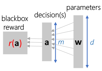
Figure 5. The black-box reward $r$ modeled as $r(\mathbf{a})$ where $\mathbf{a}=f(\mathbf{x};\mathbf{w})\in\mathbb{R}^{m}$ but $\mathbf{w}\in\mathbb{R}^{d}$; in practice, $d\gg m$.

4.1. Intuition behind the Algorithms

The key challenge with the problem is black-box access to the reward function, which disallows standard white-box optimization methods like gradient-descent. However, over the years, optimization literature has shown that for maximizing a given reward function, we do not require the exact gradient. Instead, as long as we can compute an unbiased estimate of the gradient, we can still allow strong optimization methods. Several existing methods show that we can estimate unbiased gradient of a function by only black-box queries of the function at random points (Flaxman et al., 2005; Ghadimi and Lan, 2013; Shamir, 2017).

Our key insight is that we can produce more accurate estimates of the gradients by exploiting the structure of the sketch, i.e. of the function to be learned. Recall that, we get reward $r(\mathbf{a})$ for action/decision-values $\mathbf{a}\in\mathbb{R}^{m}$, where $\mathbf{a}=f(\mathbf{x};\mathbf{w})$ for some sketch function $f$ (like linear function or decision-tree function) parameterized by weights $\mathbf{w}$ of dimension $d$ and the input features $\mathbf{x}$ are of dimension $p$. Now, if we use standard gradient estimates w.r.t. $\mathbf{w}$ then the error depends on the dimensionality $d$ of $\mathbf{w}$ due to random perturbation in each coordinate.

However, as the black-box acts only on $m$-dimensional decision values $\mathbf{a}$, we can use chain-rule and the fact that we know sketch function $f$ completely to produce a significantly more accurate estimate of the gradient that is dependent only on dimensionality of $m$ of decision-values. In several real-world codebases we observe that $m\ll d$, and hence this technique is significantly more accurate.

If the decision function is a tree, then there are additional challenges due to non-smooth and piece-wise linear nature of such functions. We propose a differentiable and shallow neural network model, and show that under some structural constraints, it implicitly represents decision trees. Then, we learn the parameters of the shallow neural network using gradient descent, with the perturbation trick. We also show that the framework is theoretically-founded —in cases when the rewards satisfy nice properties, the parameters learnt, and in turn the synthesized code, is optimal in a precise sense.

4.2. Learning constants ($f\in\textsc{Const}$)

We first consider synthesis with Const language, which reduces to learning a set of constants, without any features. That is, in this case, the decision values given by the synthesized program ($\mathbf{a}$) are just the model parameters, i.e., $\mathbf{a}=\mathbf{w}$, and hence $m=d$. See Figure 1 (left) for an example of such a sketch.

For Const language the problem reduces to the standard online learning with bandit feedback problem, which can be solved using a randomized gradient descent algorithm proposed by (Flaxman et al., 2005) (see Algorithm 2). Note that line $3$ of the algorithm first estimates the gradient at $\mathbf{a}^{(t)}$ by using random perturbation $\mathbf{u}$ and then performs standard gradient ascent (because we are maximizing reward) over $\mathbf{a}$ using the estimated gradient. Also, while Algorithm 2 mostly follows template of Algorithm 1, there is a minor difference which is that the reward function is not queried at the predicted decision value $\mathbf{a}^{(t)}$, instead it is queried at a perturbation of $\mathbf{a}^{(t)}$.

Algorithm 2 Learning constants

1:procedure UpdateConstantModel (Input: $\mathbf{x}^{(t)}$, $\eta$, $\delta$)

2:     Sample $\mathbf{u}$ uniformly from $\{\mathbf{u}\ |\ \|\mathbf{u}\|_{2}=1\}$

3:     $\mathbf{a}^{(t+1)}=\mathbf{a}^{(t)}+\eta\frac{1}{\delta}r(\mathbf{a}^{(t)}+\delta\mathbf{u})\mathbf{u}$

Note that in this language, there is no input context/features $\mathbf{x}$, hence $p=0$. Also, the number of decision values is same as the number of parameters $d$. It is easy to see that the update complexity of the method is only $O(d)$. Below we formally state the sample complexity as well under certain assumptions that we define first.

Definition 6 (Concavity).

The reward function $r$ is said to be concave if, for all $\mathbf{a},\mathbf{a}^{\prime}\in\mathbb{R}^{m}$ and $\lambda\in[0,1]$,

$$r\big{(}\lambda\mathbf{a}+(1-\lambda)\mathbf{a}^{\prime}\big{)}\geq\lambda r(\mathbf{a})+(1-\lambda)r(\mathbf{a}^{\prime})\ .$$

Definition 7 (Lipschitz-continuity).

The reward function $r$ is said to be $L$-Lipschitz continuous if for all $\mathbf{a},\mathbf{a}^{\prime}\in\mathbb{R}^{m}$,

$$|r(\mathbf{a})-r(\mathbf{a}^{\prime})|\leq L\|\mathbf{a}-\mathbf{a}^{\prime}\|_{2}\ .$$

Theorem 1 ((Flaxman et al., 2005)).

Assume the reward function $r$ is concave (Definition 6) and Lipschitz continuous (Definition 7). At the end of $T$ rounds, Algorithm 2 satisfies:

$$R_{T}\leq C\cdot\frac{m}{T^{1/4}}\ ,$$

where $C>0$ is a global constant.

That is, to ensure $R_{T}\leq\epsilon$, the sample complexity of the algorithm is $O(m^{4}/\epsilon^{4})$. The above bound can be further improved in settings (e.g. offline) where it is possible to obtain reward $r(\mathbf{a})$ at two different $\mathbf{a}$ values. In that case, the gradient estimator in Step 4 of Algorithm 2 can be replaced with:

(2) $$\mathbf{a}^{(t+1)}=\mathbf{a}^{(t)}+\eta\frac{1}{\delta}(r(\mathbf{a}^{(t)}+\delta\mathbf{u})-r(\mathbf{a}^{(t)}-\delta\mathbf{u}))\mathbf{u}.$$

And the bound can be improved (Shamir, 2017) as stated below.

Theorem 2 ((Shamir, 2017)).

Assume the reward function $r$ is concave (Definition 6) and Lipschitz continuous (Definition 7). At the end of $T$ rounds, Algorithm 2, with the “two-point” gradient estimator (2) in Step 4, satisfies:

$$R_{T}\leq C\cdot\frac{m}{T^{1/2}}\ ,$$

where $C>0$ is a global constant.

That is, in the offline setting, the rate of convergence wrt $T$ improves significantly which is critical for deployment of such solutions as the reward computation in general is expensive. Furthermore, note that both the regret bounds suffer from a linear dependence on the number of constants to learn ($d=m$) which is tight as the method is required to explore $r(\mathbf{a})$ in all the $m$ coordinates to accurately estimate the gradient. So, if in the extreme case, if every parameter to tune in the system is treated as individual constants, irrespective of the decision outcome’s structure, then $m=d$ which is expensive; typically number of outcomes $m$ is an order of magnitude smaller than the number of parameters $d$. The next two sub-sections discuss how one can exploit additional structure in certain templates, when applicable, to reduce the dependence on $d$.

4.3. Learning linear models ($f\in\textsc{Linear}$)

Now let us consider the problem of synthesizing programs from the Linearlanguage, where the decisions $\mathbf{a}$ are fixed to be a linear function of some observed features $\mathbf{x}$. That is, $\mathbf{a}=f(\mathbf{x};\mathbf{w})$ where $f$ is a fixed linear function and $\mathbf{x}$ are the observed features/context. Note that unlike in Section 4.2 where $\mathbf{a}$ were fixed to be constant despite changing context of the system ($\mathbf{x}$), in this case, we allow $\mathbf{a}$ to change as a linear function of the features $\mathbf{x}$.

Following the online setting described in Section 2, we observe features $\mathbf{x}^{(t)}\in\mathbb{R}^{p}$ in the $t$-th round and provide decision values $\mathbf{a}^{(t)}\in\mathbb{R}^{m}$ given by $\mathbf{a}^{(t)}=\mathbf{w}^{(t)}\mathbf{x}^{(t)}$ where $\mathbf{w}^{(t)}\in\mathbb{R}^{m\times p}$. The black-box system $B$ then provides reward $r^{(t)}(\mathbf{a}^{(t)})$ for the predicted $\mathbf{a}^{(t)}$, and the parameters $\mathbf{w}$ are then updated based on the reward. Thus the regret is defined for this problem as:

(3) $$R_{T}:=\ \ \max_{\mathbf{w}}\frac{1}{T}\sum_{t=1}^{T}r\big{(}f(\mathbf{x};\mathbf{w})\big{)}-\frac{1}{T}\mathbb{E}\bigg{[}\sum_{t=1}^{T}r\big{(}f(\mathbf{x};\mathbf{w}^{(t)})\big{)}\bigg{]}.$$

Note that in this case, the number of parameters $d=m\times p$ which can be very large as in typical systems, we would require several features to capture the context of the system. This is illustrated in Figure 5. If we treat $\mathbf{w}$ as constants to be learned and apply Algorithm 2 with rewards $\widetilde{r}(\mathbf{w}^{(t)})=r(\mathbf{w}^{(t)}\mathbf{x}^{(t)})$, the regret for such a method would scale as $d/T^{1/4}=m\cdot p/T^{1/4}$. On the other hand, $m$ which is the total number of decisions $\mathbf{a}$ to be estimated tends to be significantly smaller (typically $<\sim 10$). So the question is if we can devise an algorithm that scales better with $d$ when $m\ll d$.

Algorithm 3 Learning linear models

1:procedure UpdateLinearModel (Input: $\mathbf{x}^{(t)}$, $\eta$, $\delta$)

2:     Define $\mathbf{a}^{(t)}:=\mathbf{w}^{(t)}\mathbf{x}^{(t)}\in\mathbb{R}^{m}$, where $\mathbf{x}^{(t)}\in\mathbb{R}^{p}$ and $\mathbf{w}^{(t)}\in\mathbb{R}^{m\times p}$

3:     Sample $\mathbf{u}\in\mathbb{R}^{m}$ uniformly from $\{\mathbf{u}\ |\ \|\mathbf{u}\|_{2}=1\}$

4:     $\mathbf{w}^{(t+1)}=\mathbf{w}^{(t)}+\eta\frac{m}{\delta}r(\mathbf{a}^{(t)}+\delta u)\mathbf{u}\cdot(\mathbf{x}^{(t)})^{\text{T}}$

We exploit the linear structure of the template to significantly reduce the regret and hence the number of samples required to obtain good estimate of $\mathbf{a}$. We make the following simple observation: $\nabla_{\mathbf{w}}r(\mathbf{x}^{(t)}\mathbf{w})=\mathbf{x}^{(t)}(\nabla_{\mathbf{a}}r(\mathbf{a}))^{\text{T}}$ where $\mathbf{a}:=\mathbf{w}\mathbf{x}^{(t)}$ and $(b)^{\text{T}}$ is the transpose of $b$. Hence, the gradient wrt $\mathbf{w}$ has a special form that requires estimating only a $m$ dimensional vector $\nabla_{\mathbf{a}}r(\mathbf{a})$ instead of a $m\times p$-dimensional matrix. This leads to significantly cheaper gradient estimation step, implying a tighter regret bound and sample complexity that we discuss below. Also, note that the update complexity of the method is $O(mp)$, which is optimal.

Our novel algorithm for updating $\mathbf{w}$ is given in Algorithm 3 and the regret of the algorithm is given by:

Theorem 3.

Let $r$ be concave and Lipschitz continuous. Then the regret defined in Equation 3 for Algorithm 3 can be bounded as:

$$R_{T}=\max_{\mathbf{w}}\frac{1}{T}\sum_{t=1}^{T}r\big{(}\mathbf{w}\mathbf{x}^{(t)}\big{)}-\frac{1}{T}\mathbb{E}\bigg{[}\sum_{t=1}^{T}r\big{(}\mathbf{w}^{(t)}\mathbf{x}^{(t)}\big{)}\bigg{]}\leq O\bigg{(}\frac{m}{T^{1/4}}\cdot\sqrt{\max_{t}\|\mathbf{x}^{(t)}\|_{2}}\bigg{)}\ .$$

The above regret bound implies sample complexity bound of $O(m/\epsilon^{4})$ to ensure regret of $\epsilon$. The proof of the theorem relies on Lemma 3.1 of (Flaxman et al., 2005); but the key observation we make is that the norm of the noise in the gradient in Step 5 of Algorithm 3 is bounded by $O(m)$ rather than $O(d)$, if we appropriately choose $\delta$ and $\eta$ at line 4. See Appendix B for details. Note that the above regret bound is dependent only on $m$ and is completely independent of $d$ given $m$. Dependence on $d$ (through $p$) can creep through $\|\mathbf{x}^{(t)}\|_{2}$ but several practical problems tend to have small $\|\mathbf{x}^{(t)}\|_{2}$ and in general such a bound is considered to be “dimension independent”. In contrast, the regret of Algorithm 2 is bound to suffer a linear dependence on $d=mp$. This implies significantly smaller regret for Algorithm 3 for $m\ll d$ which is a typical case in practical applications. Finally, similar to the previous section, in the offline deployment setting with two-point feedback, the regret bound decreases at $T^{-1/2}$ rate.

4.4. Learning tree models ($f\in\textsc{Imp}$)

In this section, we discuss our method for synthesizing a program from the general Imp language. As discussed in Section 2, the problem is equivalent to that of learning a general decision tree with rewards, which is a challenging problem and has been relatively unexplored in both machine learning and programming languages literature.

Recall that the decisions $\mathbf{a}$ are fixed to be a function $f$ of the context ($\mathbf{x}\in\mathbb{R}^{p}$), where $f$ is a tree structured function, i.e., $\mathbf{a}=f(\mathbf{x};\mathbf{w})$ with $f$ being a decision tree parameterized by $\mathbf{w}$.

As in Algorithm 1, the learner would observe $\mathbf{x}^{(t)}$ in the $t$-th round, propose $\mathbf{w}^{(t)}$ to predict decisions $\mathbf{a}^{(t)}$, receive reward $r(\mathbf{a}^{(t)})$ and the goal is to optimize the reward. If we ignore the tree structure of $\mathbf{a}$ and treat $\mathbf{w}$ as the parameters to be learned using constant template and apply Algorithm 2, it would lead to poor regret and hence many rounds for learning a good solution (as discussed in linear templates). The reason is that the size of $\mathbf{w}$ typically increases exponentially with the height of the tree, which implies that the regret bound of Section 4.2 would also increase exponentially with the height of the tree.

Instead, we use the following observation, that we exploited in the previous section as well (for simplicity we provide this observation when $a\in\mathbb{R}$ is a scalar):

$$\nabla_{\mathbf{w}}r(f(\mathbf{x}^{(t)};\mathbf{w}^{(t)}))=r^{\prime}(a^{(t)})\nabla_{\mathbf{w}}f(\mathbf{x}^{(t)};\mathbf{w}^{(t)}),$$

where $\nabla_{\mathbf{w}}r(f(\mathbf{x}^{(t)};\mathbf{w}^{(t)}))$ is the derivative of $r(\cdot)$ wrt $\mathbf{w}$, evaluated at $\mathbf{w}^{(t)}$. Now, $r^{\prime}(a)$ is the first derivative of $r$ evaluated at $a^{(t)}=f(\mathbf{x}^{(t)};\mathbf{w}^{(t)})$ and $\nabla_{\mathbf{w}}f(\cdot)$ is the derivative of $f(\cdot)$ wrt $\mathbf{w}$.

Note that we do not know function $r$ and can only receive feedback $r(\mathbf{a}^{(t)})$, so $r^{\prime}$ would be computed using the standard perturbation based technique (see Algorithm 2). However, as we know function $f$, we can evaluate $\nabla_{\mathbf{w}}f(\cdot)$ accurately assuming $f$ represents a differentiable tree function. Together, this can significantly reduce the number of prediction-reward feedback loops for learning the template, even though the number of parameters $\mathbf{w}$ can be very large — as $r^{\prime}$ is a one-dimensional quantity (and in general $m$ dimensional where $\mathbf{a}\in\mathbb{R}^{m}$) and only very few random perturbations are required for its accurate estimation. The key challenge here is that the algorithm requires computing gradient of $f(\cdot)$ wrt $\mathbf{w}$ which in general is a challenging task due to the discrete structure of trees. In this work, we develop a novel differentiable model for trees.

4.4.1. Decision Trees as Shallow Nets

The core idea of our approach and the motivation are as follows. Learning decision tree models is intractable in general, and is hard even for well-behaved known reward functions, because: (a) it is highly non-smooth and (b) the function class is piecewise-constant (or piecewise-linear). Existing approaches typically try to solve the problem greedily (Carreira-Perpinán and Tavallali, 2018) or try to come up with a smooth relaxation or upper bound of the loss function (Norouzi et al., 2015). A major shortcoming of these techniques is that they are tied to a specific loss (reward) function or type of decisions made and therefore do not extend to more general settings.

Our non-greedy approach uses a differentiable and shallow neural network model for learning decision trees and works with any general loss/reward function. Moreover, we can formally show that the neural network architecture under some structural constraints is equivalent for decision trees, thus allowing gradient based training methods for learning tree parameters. We refer to this model as EntropyNet, denoted by $f_{\emph{{Net}}}$. The details of this approach are given in Appendix A.

Algorithm 4 Learning trees in $\mathsf{PBR}$

1:procedure LearnInRounds (Input: $h$)

2:     Initialize EntropyNet $f_{\emph{{Net}}}$ parameters (vectorized) $\widetilde{\mathbf{w}}^{(0)}\in\mathbb{R}^{d}$ for the given height $h$

3:     Choose $\delta>0$, and learning rate $\eta$

4:     for $t=0,1,2,\dots$ do

5:         Observe features $\mathbf{x}^{(t)}:=[x_{1},x_{2},\dots,x_{p}]$

6:         Define $a^{(t)}:=f_{\emph{{Net}}}(\mathbf{x}^{(t)},\mathbf{w}^{(t)})\in\mathbb{R}$, where $\mathbf{x}^{(t)}\in\mathbb{R}^{p}$ are input features

7:         Sample $u\in\mathbb{R}$ uniformly from $\{-1,1\}$

8:         Update $\widetilde{\mathbf{w}}^{(t+1)}=\widetilde{\mathbf{w}}^{(t)}+\frac{\eta}{\delta}r(a^{(t)}+\delta u)u\cdot\nabla_{\widetilde{\mathbf{w}}}f_{\emph{{Net}}}(\mathbf{x}^{(t)},\widetilde{\mathbf{w}}^{(t)})$      

9:     return Tree model (Definition 4) $\mathbf{W},\bm{\Theta}=\textsc{InferTree}(\widetilde{\mathbf{w}},h)$ (Algorithm 5 in Appendix B)

Algorithm. We provide the pseudo-code for learning trees, for the case when $a\in\mathbb{R}$, in Algorithm 4 (which also subsumes the basic skeleton in Algorithm 1) but it can be easily extended to the general decision functions in Imp (that return $m$ values instead of 1). Note that the algorithm learns parameters for the equivalent function $f_{\emph{{Net}}}$ and eventually returns the intended decision tree function (which can be easily inferred given $f_{\emph{{Net}}}$ via InferTree procedure stated in the Appendix B). While intuitively exploiting the tree structure should lead to significantly smaller regret bound, it is difficult to provide a rigorous analysis of the same. Due to tree structure $f(\cdot)$ being a non-convex function, the standard online learning techniques (Flaxman et al., 2005) do not apply in this case. While certain novel techniques like (Agarwal et al., 2019) have been designed for non-convex optimization, we leave further investigation into the regret bound and hence the sample complexity of this method for future work.

4.5. PBR usage in practice

Here we briefly discuss how our PBR method can be applied in real-world codebases. At a high level, the programmer must first decide the set of decision values that are critical to the performance of the system, and also figure out the context/features important for setting the decision values. Then, the programmer sets up a reward function based on critical metrics that needs to be optimized. Finally, the programmer can either specify the language (Const, Linear, Imp) from which a program should be synthesized. Our tool takes care of storing the feature values and the corresponding reward functions, and learning the appropriate decision function. See Appendix D for more details about the front-end that enables using our PBR method easier for developers. Note that our exposition focus only on setting where programmer does not provide any partial sketch; further empirical validation of our methods in partial sketching settings is left for future work.

While our sample complexity bounds hold only for Lipschitz continuous and concave functions, in practice the functions might have discontinuities. However, we observe empirically that our method is indeed able to learn effective function/sketch parameters. We attribute this to the fact that in practice, the reward function would have a few points of discontinuities (Chaudhuri et al., 2012), thus the sample complexity is small in large portions of the parameter space. Furthermore, perhaps the first order or second order optima (instead of global optima) are also reasonably good solutions, which can be ensured by techniques similar to our method (Agarwal et al., 2019). We leave rigorous analysis of practical reward functions and our methods in those settings to future work.

5. Implementation and Evaluation

In this section, we discuss implementation and present empirical evaluation of our algorithms. Our algorithms for the $\mathsf{PBR}$ framework operate in both online and offline settings requiring only black-box access to the reward function, and the key benefit of our algorithms is in settings where the structure of the decision function/sketch (linear or tree) can be exploited. We design evaluation studies that bring out some of these aspects and merits under different settings. In particular, we seek answers to the following questions.

1. In practice, how well do our algorithms help learn decision functions in codebases with complex reward functions? In this study, we apply our algorithms to synthesize search and ranking heuristics in the widely-used (PROSE, 2015) codebase for synthesizing data formatting programs in the FlashFill DSL.

2. How do our (black-box) $\mathsf{PBR}$ algorithms compare with white-box synthesis techniques? As it is difficult to construct strong real-world examples of white-box reward functions, we consider somewhat artificial programs proposed by prior work (Chaudhuri et al., 2014), where the entire system, including reward function, is available as a white-box, and the reward function can be invoked as many times as desired. In this artificial setting, we compare our approach with  $\mathsf{Sketch}$ (Bodik and Solar-Lezama, 2006), which uses SAT solvers to synthesize integer valued parameters, and  Fermat (Chaudhuri et al., 2014), which synthesizes continuous valued parameters using numerical methods.

3. Does exploiting structure in the decision functions really help? Here, we want to compare our algorithms that exploit the decision function structure presented in Section 4 against treating the synthesis as a sketch with missing numerical parameters, which can be addressed using black-box reinforcement learning style methods.

Evaluation settings and baselines. We work with both online (where we need to take decisions at every round) and offline settings, and black-box rewards. We evaluate and compare  $\mathsf{PBR}$ algorithms with different baselines, each applicable only to certain settings unlike our algorithms (and therefore selectively used for comparison in the aforementioned three studies as applicable): (1) general-purpose (evolutionary) optimization algorithms in the popular open-source $\mathsf{Nevergrad}$ platform (Rapin and Teytaud, 2018), which is also applicable to black-box, offline and continuous parameter settings; and (2) the multi-arm bandit formulation (Bietti et al., 2018) that is currently used in the popular $\mathsf{DecisionService}$ (Agarwal et al., 2016), an enterprise-scale reinforcement learning framework, that works in black-box and online learning settings, but is restricted to discrete parameters/decisions (such as recommending ads or news articles to users); and (3) the $\mathsf{Sketch}$ synthesis tool (Bodik and Solar-Lezama, 2006) which is applicable to white-box and offline settings, and can synthesize integer-valued parameters; and (4) the Fermat tool (Chaudhuri et al., 2014), which is also applicable to white-box, offline settings, and can synthesize continuous-valued parameters.

5.1. Implementation

We have implemented the PBR framework (PBR.DecisionFunction and PBR.AssignReward API introduced in Section 2), and the learning algorithms presented in Section 4 as a utility library (with support for C# and Python languages) for software developers. Our implementation also provides flexibility and customization capabilities to the developer in terms of explicitly providing domain knowledge (for example, the developer can suggest one of Imp, Const or Linear to synthesize an appropriate decision function) and ability to inspect and debug the synthesized code for the decision function (instead of working with the tree or linear model as a black-box). Details of the API are given in Appendix D. All experiments are conducted on a standard desktop machine with 16GB RAM, 2GHz processor and 4 cores.

5.2. How well do our algorithms help learn decision functions in real codebases with complex reward functions?

PROSE (PROSE, 2015) is a well-known framework for programming by examples (PBE). It has been instrumental in developing software for many practical applications around data ingestion (Raza and Gulwani, 2018; Iyer et al., 2019), formatting, spreadsheet processing (Gulwani, 2011), web extraction, program repair and transformation (Le et al., 2017; Rolim et al., 2017), and more. PROSE provides a meta-framework (Polozov and Gulwani, 2015) for (a) defining a domain-specific language (DSL) for programs of interest, (b) synthesizing programs from a given input-output specification in a divide-and-conquer fashion, (c) pruning the search space, and (d) ranking the (sub)programs to narrow down to one or a few programs intended by the user. Often, software applications built over the PROSE engine require coming up with their own DSL (e.g. spreadsheet processing vs web extraction) and ranking function.

Several critical decision making points exist in the resulting software; in particular, developers write several complex heuristics for determining how to score different operators in the DSL and ranking the sub-programs that these operators compose, and in turn, for choosing the “best programs” capturing the user intent with very few input-output examples. There is a growing line of research in the intersection of programming languages and AI (Gulwani and Jain, 2017). In this study, we consider the popular spreadsheet processing application DSL (Gulwani, 2011) that has been commercially deployed (PCWorld, 2012). The corresponding ranker (available here (PROSE, 2015), details are provided in (Natarajan et al., 2019)) has several heuristic rules, each implemented as a function involving multiple hard-coded constants and features. For instance, the RegexPair rule shown in Figure 6 has three hard-coded constants.

⬇

public double RegexPair(double bias_RegexPair, double score_RegexPair_r, double score_RegexPair_r2) {

return -0.205*bias_RegexPair +

1*score_RegexPair_r + 1*score_RegexPair_r2;

}

Figure 6. The RegexPair heuristic in $\mathsf{PROSE}$ (PROSE, 2015; Natarajan et al., 2019) with parameters of interest highlighted.

We consider the problem of learning these typically hand-tuned parameters to improve the performance of PROSE as measured on a set of curated benchmark tasks (Natarajan et al., 2019). Here, the reward function is defined as the fraction of tasks for which the software synthesizes a correct program for. This reward function is highly discontinuous and complicated, and computing the function involves running the entire software with complex recursive algorithms interleaving synthesis and ranking. But, we know that the constants in the ranking functions (e.g., Figure 6) heavily influence the performance of PROSE on most of the tasks, and thus, the reward. Note that evaluating the reward function is expensive in terms of time — a single evaluation takes nearly 10 minutes. So we evaluate algorithms based on the number of reward computations (sample complexity) as well as the time taken to converge to a good solution (i.e. one that achieves good performance on the benchmark).

Recall that due to black-box nature of the reward function, existing sketch methods that require whitebox access do not apply (Bodik and Solar-Lezama, 2006; Chaudhuri et al., 2014). Instead, we compare our method against a multi-arm bandit method (UCB, as implemented in the open-source framework SMPyBandits (Besson, 2018))– a popular reinforcement learning style method. However, UCB requires discretization of the real-valued parameters into a small number of actions, which means that the number of actions grows exponentially with the number of parameters and can be tricky when tuning parameter values of high precision. In this case, we discretize each parameter value into 9 bins around 0 (which is a good initial solution). This implies that just for one of the heuristics (RegexPair mentioned above), the total number of actions (from which UCB chooses one set of decision-value/action) turn out to be $729$. So, to ensure applicability of the UCB method, we initially focus only on learning one heuristic function in PROSE codebase.

Figure 7 (a) shows the comparison of $\mathsf{PBR}$ and UCB algorithms for learning the three parameters associated with the RegexPair function (Figure 6). We observe that (a) $\mathsf{PBR}$ quickly ramps up the reward in about 50 queries (in about 6 hours), whereas the UCB algorithm spends a lot of time and queries performing “explore-exploit” of multiple independent actions, without gaining enough confidence on any particular action. Even if we reduce the action space of UCB to 125 actions (i.e. discretize each parameter into 5 bins instead of 9), the performance of UCB is still significantly worse than $\mathsf{PBR}$ as observed from Figure 16 (in Appendix C). The observations are similar in Figure 7 (b) that shows a comparison for synthesizing the FormatDateTimeRange function (Figure 15 in Appendix C) which has a larger number of parameters to learn.

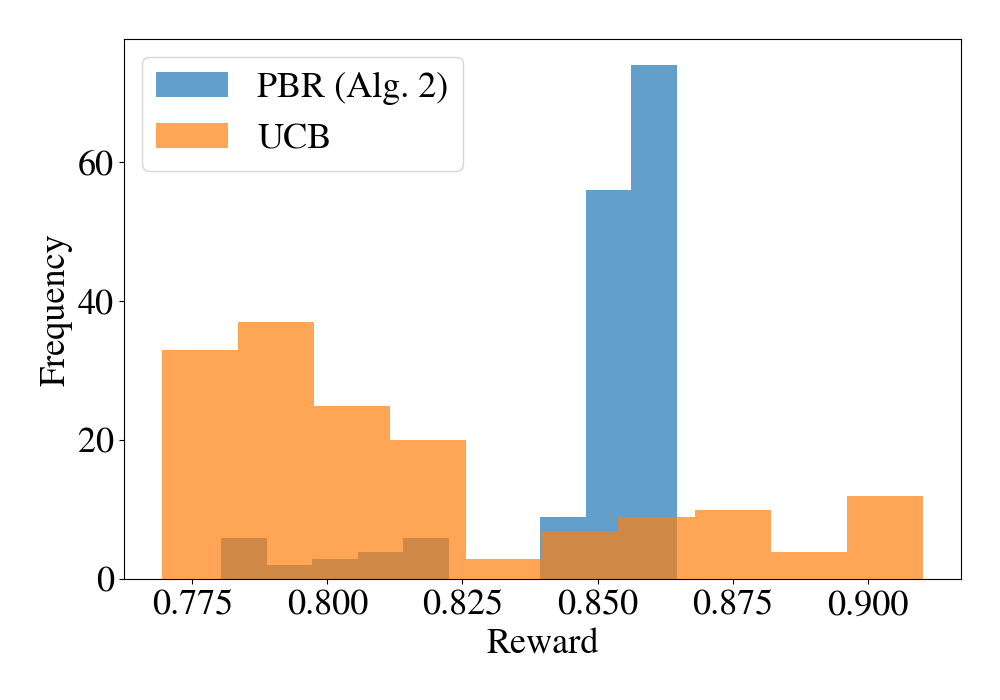
Figure 17. Distribution of rewards received by $\mathsf{PBR}$ and UCB when tuning RegexPair parameters (Figure 6), corresponding to the result in Figure 7 (a).

An important aspect of evaluation of parameter learning is how often the software or the system that is tuned is exposed to “bad” rewards. We find that $\mathsf{PBR}$ spends much smaller fraction of time with low rewards as against UCB (Figures 17 and 18 in Appendix C).

Deployment. Next, we deployed our $\mathsf{PBR}$ framework to jointly learn the parameters ($d=490$) for all the ranking heuristics/decisions ($m=70$) in the $\mathsf{PROSE}$ codebase for spreadsheet processing DSL. At convergence (after nearly 100 hours, 250 queries), we observed that the parameters learnt by $\mathsf{PBR}$ improved the correctness of the system by nearly 8% compared to the state-of-the-art results (Natarajan et al., 2019) on the benchmark consisting of 740 tasks. In particular, with the learnt parameters, $\mathsf{PROSE}$ system achieved an accuracy of 668/740 compared to 606/740 obtained by (Natarajan et al., 2019), and 703/740 obtained by domain experts over multiple years by hand-tuning heuristics in the PROSE codebase today. A key factor for success of $\mathsf{PBR}$ here is that it optimizes for the metric of interest directly, in contrast to the ML approach in (Natarajan et al., 2019). Finally, note that we couldn’t apply UCB method for learning all the $70$ decision functions as it requires discretization of the entire decision-value space which leads to exponential blow-up.

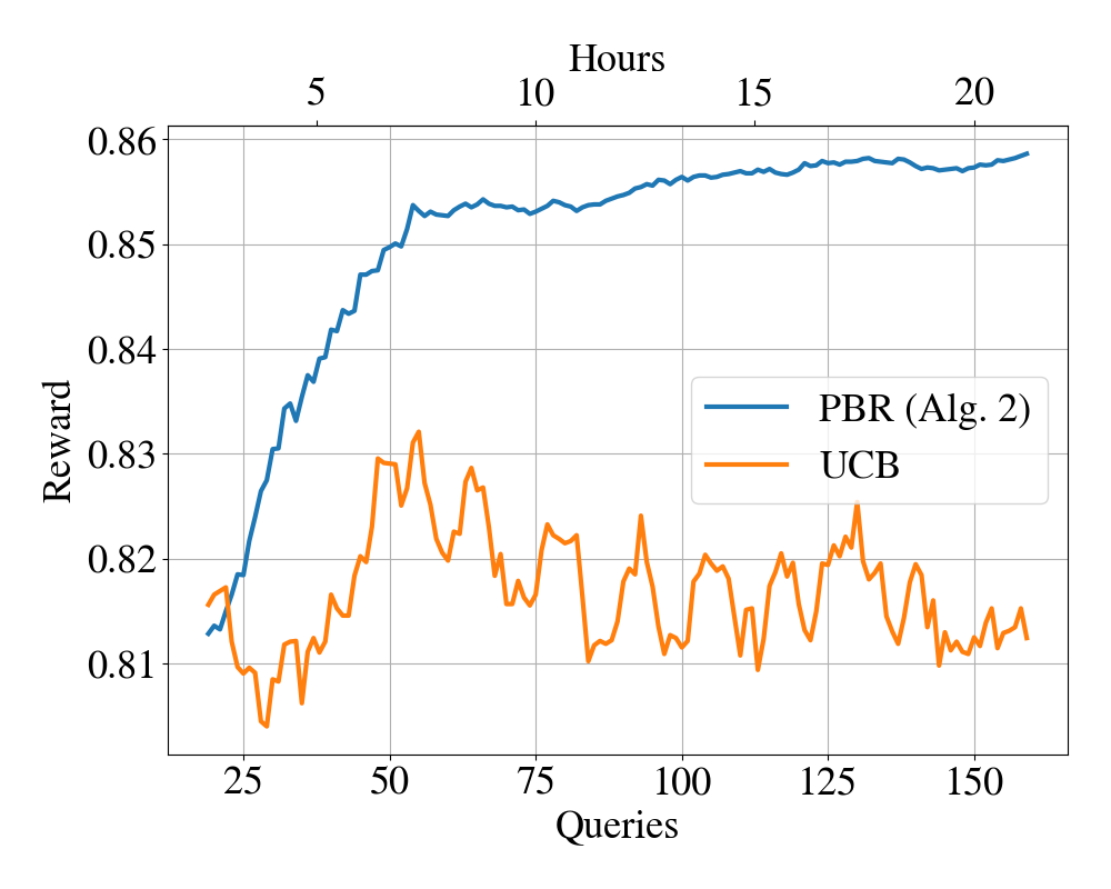
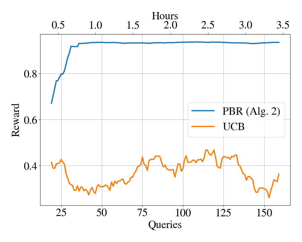
(a)	(b)

Figure 7. (Smoothed) Reward over time wrt number of calls to reward oracle to learn different functions in $\mathsf{PROSE}$. For the multi-arm bandit formulation (UCB), we discretize each parameter before execution. (a): Learning RegexPair with $3$ parameters (Figure 6). For UCB, we discretize each parameter into $9$ values resulting in $9*9*9=729$ actions. The sample complexity of UCB is quite high and the solution it obtains is relatively poor even after nearly 1 day. (b) Learning FormatDateTimeRange with $10$ parameters (Figure 15 in Appendix C). For UCB, we discretize each parameter into $5$ values resulting in $5^{10}\sim 9$ million actions.

5.3. How do our algorithms compare with white-box synthesis techniques?

Here we compare $\mathsf{PBR}$ to program synthesis techniques such as  $\mathsf{Sketch}$ (Bodik and Solar-Lezama, 2006), which synthesizes parameter values for integer holes using CEGIS techniques implemented on top of SAT/SMT solvers, and Fermat (Chaudhuri et al., 2014), which synthesizes continuous-valued parameters using numerical methods. We also compare with a optimization algorithm implemented in the open-source $\mathsf{Nevergrad}$ platform (Rapin and Teytaud, 2018). Specifically, we use TBPSA, an evolutionary algorithm that can perform well in continuous, stochastic settings (T. Cazenave, 2019). While our methods allow for realstic settings of online and blackbox rewards, but to ensure fair comparison against existing methods, we restrict this set of experiment to restricted and artificial contexts where we have white-box access to the entire system, including the reward function, and the reward function can be invoked as many times as desired.

First, we generate problems of the following type, where the goal is to learn a Linear decision function $f(\cdot;\mathbf{w})$, with integral $\mathbf{w}\in\mathbb{Z}^{d}$, such that the following expected reward is maximized:

(4) $$\max_{\mathbf{w}\in\mathbb{Z}^{d}}\mathbb{E}[r\big{(}\mathbf{w}\cdot\mathbf{x}\big{)}],$$

where the expectation is with respect to randomness in the features $\mathbf{x}$ and the reward $r(.)$ is set to be negative of loss $\ell$ (minimizing the loss is equivalent to maximizing the reward), defined below:

(5) $$\ell_{\text{sq}}(y):=\big{(}y-y^{*}\big{)}^{2},\text{ or }\ell_{\text{abs}}(y):=\big{|}y-y^{*}\big{|}.$$

The values $y^{*}$ are chosen to be such that $y^{*}=\mathbf{w}^{*}\cdot\mathbf{x}$ for some fixed $\mathbf{w}^{*}\in[0,1,2,\dots,10]^{d}$ which is the optimal solution to the problem (4). We assume a uniform distribution over $n$ features $\mathbf{x}$ to compute the expectation in  (4). We fix $n=2d$ in all cases (which is sufficient for learning).

The $\mathsf{Sketch}$ implementation is given in Figure 19 (Appendix C.2). For $\mathsf{PBR}$, we use Algorithm 3 (fixing $\delta=0.5$ and $\eta=2\times 10^{-3}$) meant for Linear decision functions.

Remark 3.

We restrict the search space for $\mathsf{Sketch}$ further by ensuring that $\mathbf{w}^{*}$ values are non-negative (requirement of the tool), small and bounded; we explicitly add these bound constraints in the  $\mathsf{Sketch}$ problem specification. See the assertion in Figure 19. Furthermore, in all the experiments, we work with 4-bit integers for holes, which we know is sufficient, using the flag bnd-cbits in the $\mathsf{Sketch}$ tool. Using larger-sized integers will only increase the computation time.

We create multiple problem sets varying number of parameters $d$ in Equation (4). To account for randomness in algorithms as well as in problem sets themselves, we repeat each experiment 10 times and report (a) accuracy, i.e. how often does the method solve the problem (4) exactly, and (b) mean and standard deviation of time taken to solve. Results are presented in Table 1, for the two loss functions given in (5). It is clear that the search algorithm of sketching takes prohibitively long time, and fails to solve the problem even for small values of $d$ within the budget of 1 hour (and in many cases, we find that the tool prematurely fails well before the timeout despite multiple restarts with random seeds). In case of squared loss $\ell_{\text{sq}}$, sketching totally fails because it involves using multiplication circuits in the back-end SAT problem. Our algorithm solves every problem instance (as guaranteed by Theorem 3). Even the general-purpose, continuous, black-box optimization algorithm of $\mathsf{Nevergrad}$ fails to compute the exact solution in most of the cases within 1 hour. The progress of $\mathsf{Nevergrad}$ and $\mathsf{PBR}$ algorithms against # reward queries is shown in Figure 8.

Table 1. Comparison of techniques on parameter learning problem in Equation (4), for the two losses defined in Equation (5), for increasing number of parameters (holes) $d$. The implementation of $\mathsf{Sketch}$ is given in Figure 19. For each $d$, we create 10 problem sets and report the mean and the standard deviation of the time taken (in seconds) to solve the problems. The number of cases successfully solved out of 10 is indicated in parentheses. Timeout is set to 1 hour.

$d$	$\ell_{\text{abs}}$			$\ell_{\text{sq}}$
	$\mathsf{Sketch}$	$\mathsf{PBR}$ (Alg. 3)	$\mathsf{Nevergrad}$	$\mathsf{Sketch}$	$\mathsf{PBR}$ (Alg. 3)	$\mathsf{Nevergrad}$
2	0.49 $\pm$ 0.04 (10)	0.04 $\pm$ 0.01 (10)	298.66 $\pm$ 555.73 (5)	70.8 $\pm$ 73.95 (10)	0.01 $\pm$ 0.00 (10)	0.41 $\pm$ 0.15 (3)
4	9.65 $\pm$ 7.72 (10)	0.04 $\pm$ 0.01 (10)	- (0)	- (0)	0.01 $\pm$ 0.00 (10)	- (0)
6	582.1 $\pm$ 425.0 (5)	0.07 $\pm$ 0.03 (10)	- (0)	- (0)	0.01 $\pm$ 0.00 (10)	- (0)
8	- (0)	0.06 $\pm$ 0.02 (10)	- (0)	- (0)	0.02 $\pm$ 0.01 (10)	- (0)

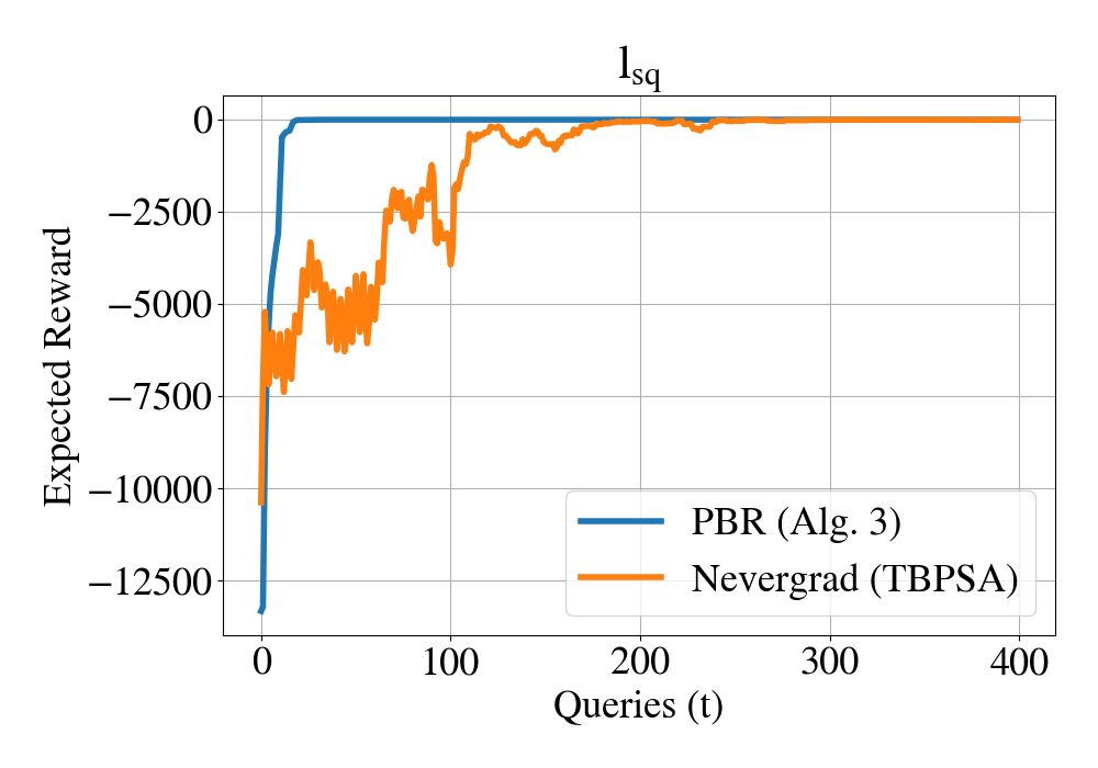
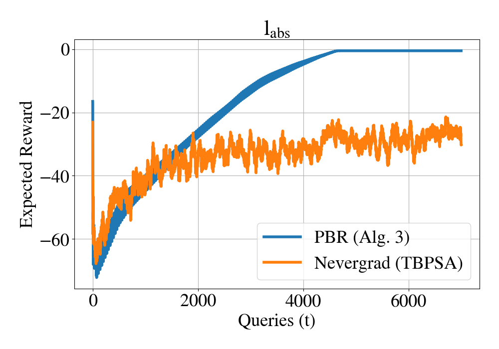
(a) Squared loss $\ell_{\text{sq}}$	(b) Abs. deviation loss $\ell_{\text{abs}}$

Figure 8. Expected reward (in problem (4)) vs. number of queries to reward $r$ for loss functions in Equation (5).

We tried to relax the sketch specification to not require exact solution to problem (4) but approximate to a small additive error; however, the sketch tool still fails (See Appendix C.2).

⬇

1double Thermostat(double lin, double ltarget) {

2 double h = ??(0, 10); double tOn = ltarget + ??(-10,0);

3 double tOff = ltarget + ??(0, 10); bool isOn = false; double K = 0.1;

4 assert(tOn < tOff; 0.9); assert(h > 0; 0.9); assert(h < 20; 0.9);

5 for (int i=0; i<40; i = i + 1) {

6 if (isOn) {

7 curL = curL + (h - K * (curL - lin)); if (curL > tOff) isOn = false;

8 } else {

9 curL = curL - K * (curL - lin); if (curL < tOn) isOn = true;

10 }

11 assert(curL < 120; 0.9);

12 }

13 return abs(curL - ltarget);

14}

Figure 9. Thermostat sketch.

Next, we compare $\mathsf{PBR}$ with the Fermat tool (Chaudhuri et al., 2014) for numerical parameter synthesis with quantitative as well as boolean specification, on the synthesis benchmarks studied in (Chaudhuri et al., 2014). In particular, their technique has white-box access to the cost function that is part of the sketch. The input to Fermat is (1) a sketch implementing a cost function that returns a real value, with some holes for constants (that need to be learned) and probabilistic assertions, and (2) a distribution of the input values. The goal is to learn values for the constants minimizing: (a) the probability that the assertions fail, and (b) the expected value of the function (which computes some notion of error).

Figure 9 shows example of such a function sketch; the Thermostat function takes two probabilistic inputs (lin and ltarget), has three holes at lines 2-4 ($\texttt{??}(c_{1},c_{2})$ denotes a hole with additional insight that the parameter is likely to lie in the interval $[c_{1},c_{2}]$ (Chaudhuri et al., 2014)), contains four assertions at lines 6, 7 and 16, and returns a double value representing the error. Given the distribution of the input variables, the goal is to find the values for the three constants, such that probability for assertions failing and the expected error are minimized.

Setting up the problem in $\mathsf{PBR}$. We model this setting in $\mathsf{PBR}$, using Algorithm 2, as follows. We generate $n=10,000$ inputs for the cost function by sampling the input distribution. We define the loss as the squared error (the value returned by the sketch cost function) plus a very high additive cost for any assertion violation (we use 1000), and set the reward $r$ to negative of this loss. We consider Algorithm 2 converged when there is no improvement in the reward for 100 iterations. Following the experiment in Chaudhuri et al. (2014), we run both Fermat and $\mathsf{PBR}$ 80 times per problem, varying the initial random seed where the search starts.

Table 2. Comparison of $\mathsf{PBR}$ with Fermat on two synthesis tasks from (Chaudhuri et al., 2014).

Benchmark	Time (minutes)		# iterations		Error
	Fermat	$\mathsf{PBR}$ (Alg. 2)	Fermat	$\mathsf{PBR}$ (Alg. 2)	Fermat	$\mathsf{PBR}$ (Alg. 2)
Thermostat	119.29 $\pm$ 98.07	5.15 $\pm$ 3.62	2999.43 $\pm$ 91.93	781.11 $\pm$ 546.42	4.61 $\pm$ 2.32	2.74 $\pm$ 0.71
Aircraft	333.57 $\pm$ 4.53	6.66 $\pm$ 1.98	4232.59 $\pm$ 313.65	994.50 $\pm$ 273.29	18.09 $\pm$ 2.89	25.22 $\pm$ 1.56

Results. We compare the tools on two problems from Chaudhuri et al. (2014): Thermostat (in Figure 9) and Aircraft (details in Appendix C.3). We look at the time taken and the number of reward queries required for the algorithms to converge to some good solution, the mean error over all 80 runs (the error of a run is expected error over all inputs). The results are given in Table 2. We observe that Fermat (a) takes much longer time to converge than $\mathsf{PBR}$, and (b) uses many more reward queries to converge. Our algorithm outperforms Fermat in the Thermostat sketch in terms of the quality of the constants learnt, but is worse in the Aircraft sketch. On the other hand, Fermat requires white-box access to the code, and its applicability is very limited.

5.4. Does exploiting structure in the decision functions really help?

We now present examples to show that our algorithms can indeed exploit structure in decision functions, in order to learn a good solution to the synthesis problem with small number of queries to the reward function $r$, even though the number of parameters $d$ may be very large. For the case of Linear decision functions, Theorem 3 provides a theoretical guarantee for how exploiting the linear structure helps in terms of sample complexity. On the contrary, for decision trees (i.e. general Imp decisions), such a rigorous analysis is difficult. To this end, we consider three different  Imp decision function instances, and empirically evaluate the tree learning Algorithm 4 against posing the tree learning problems as sketches, treating every numerical parameter in the tree as a hole, and applying the Algorithm 2 that disregards any structure.

First, we consider an Imp decision function that has the Xor structure, modeled on two features distributed as given in Figure 21 (in Appendix C). Next, we consider a more complex hypothetical tuning problem Slates, where we wish to learn a piece-wise constant threshold function based on the values of two observed features, that decides what the threshold for the input should be (these type of heuristics are common in systems). In the setup, we have 6 different possible thresholds that depend on the features as shown in Figure 22 in Appendix C. In both the cases, the reward is negative of squared loss $\ell_{\text{sq}}$ defined in Equation (5) between the actual and predicted value. Figure 10 compares the performance of learning constants directly vs. exploiting the tree structure to learn the decisions. In both cases, we observe that indeed exploiting structure helps converge to a significantly better solution using much fewer reward queries. The height of the tree learnt in Xor is 2, hence we learn $d=13$ parameters using both algorithms. For Slates we learn a tree of height 3, where $d=29$. However, in both problems, the sample complexity of Algorithm 4 is proportional to $m=1$ since only one decision is made.

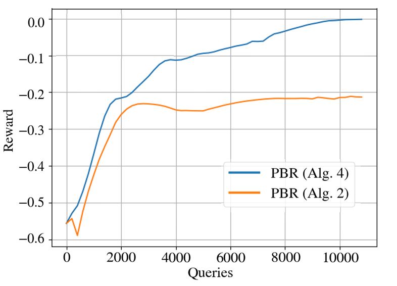
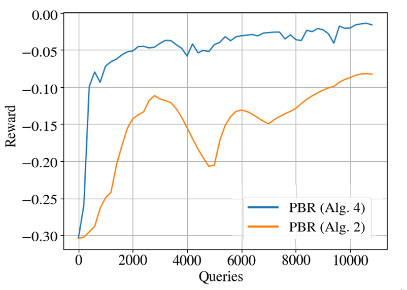
Figure 10. Reward vs number of queries to reward $r$ for learning two different tree decision functions using Algorithm 4 and Algorithm 2. (a): (Xor in Figure 21) The learnt decision function is given in Figure 23 (Appendix C); (b): (Slates in Figure 22) The learnt decision function is given in Figure 24 (Appendix C).

Next, we consider the Parrot synthesis benchmark studied by Bornholt et al. (2016); Esmaeilzadeh et al. (2012), where the goal is to learn a piece-wise polynomial approximation for the complex function in Figure 11(a) (which is more efficient to execute than the trigonometric functions). Here, we compute 16 features $\{x^{i}\cdot y^{j}\}$ for $0\leq i,j\leq 3$ based on the input $x$ and $y$ to the function that needs to be approximated. The feature distribution is uniform over $100$ pairs $(x_{i},y_{i})$ sampled from the range $[-1,1]\times[-1,1]$. We then learn a decision tree of height $h=4$ using the same $\ell_{\text{sq}}$ loss as in the above instances. We also learn the $d$ tree parameters treating them as constants, where $d=(2^{h+1}-1)*16=496$. Figure 11(b) shows expected reward against the number of queries for the two algorithms. Again, we observe that exploiting structure results in the algorithm converging to much better rewards quicker. Additionally, we observe $33\%$ and $212\%$ median percent (relative) approximation error, for Algorithm 4 and Algorithm 2, respectively.

⬇

float inversek2j(float x,float y) {

float th2 = acos(((x*x) + (y*y) - 0.5) /

0.5);

return asin((y*(0.5 + 0.5*cos(th2)) -

0.5*x*sin(th2)) /

(x*x + y*y));

}

(a)

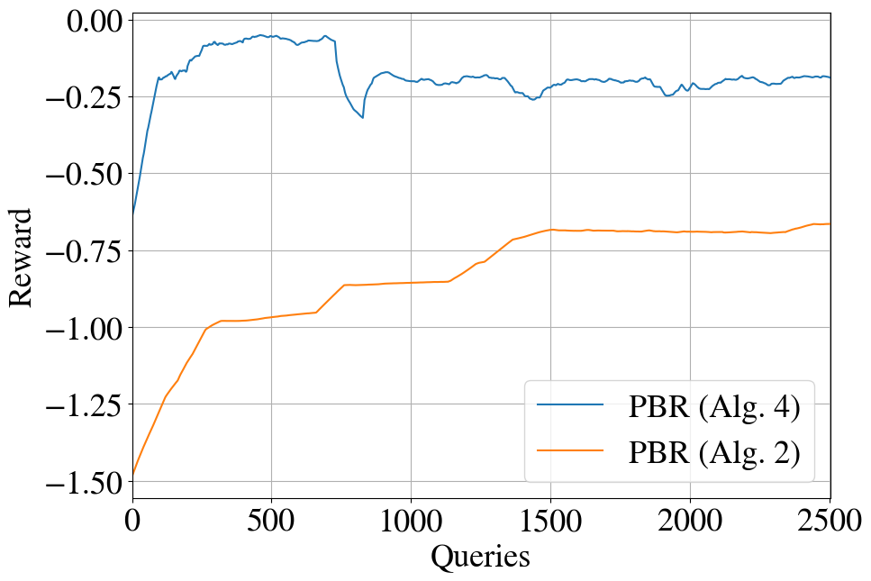
(b)

Figure 11. (a) The function to approximate from the Parrot benchmark. (b) The rewards obtained for learning the function approximations using tree model (Alg. 4) and constants (Alg. 2).

6. Related Work

A/B and Multiworld Testing. A/B testing methodology is commonly used in many disciplines and domains (medicine, especially) for understanding the effects of treatments in a controlled setting. It has been increasingly adopted in understanding the effects of parameters in systems and software (Kohavi and Longbotham, 2017; Johari et al., 2017). Performing randomized experiments on real systems, gathering data from control and treatment groups, analyzing how the parameters affect the metrics of interest, and making decisions can be disruptive, laborious, and prohibitively expensive in terms of time (especially when the number of parameters is large and continuous-valued). Multiworld testing (MWT) significantly improves upon A/B testing methodology by reusing data and context collected from a deployed system to estimate the outcome of many A/B tests without running separate tests for each; however, it still does not scale well with respect to number of parameters. The state-of-the-art MWT framework known as $\mathsf{DecisionService}$ (Agarwal et al., 2016), and is primarily intended for making a single categorical decision (such as recommending ads or news articles to users), using contextual bandit algorithms (Bietti et al., 2018). As we demonstrated in Section 5.2, the multi-arm bandit algorithms scale poorly when the multi-dimensional action space is discretized. There is recent work on extending the techniques to continuous-valued parameters (Krishnamurthy et al., 2019) and multiple parameters. However, these algorithms are yet to be incorporated into tools for efficient parameter tuning.

Reinforcement Learning (RL) is a popular and widely-used approach (Sutton and Barto, 2011) for online learning of actions/decisions in order to maximize some long-term reward. $\mathsf{SmartChoices}$ by Google (Carbune et al., 2019) is a recent example of an RL-based framework, which is primarily intended for tuning parameters in software. Similar to $\mathsf{PBR}$, their interface is developer-friendly and intuitive. Since they rely on standard RL techniques and complex neural network models, the sample complexity and reward computations required are generally high and the framework forgoes interpretability which is a key differentiating aspect in our work. Another recent line of RL research involves learning interpretable policies (as programs) (Verma et al., 2019; Verma et al., 2018) that exploit gradient-based techniques for finding a policy that optimizes some expected reward function and combinatorial search techniques for inferring the program corresponding to the policy.

Configuration Optimization in Software. An important line of related work in empirical software engineering involves automatic parameter tuning and large-scale configuration optimization (Sayyad et al., 2013; Siegmund et al., 2015; Guo et al., 2018; Kaltenecker et al., 2019; Bao et al., 2019). Our work chiefly differs from a majority of approaches in this line of work in that (a) we focus on synthesizing interpretable code for computing decisions, via learning parameters, in software, and (b) our algorithms work with arbitrary and complex reward functions in practice. In contrast, for example,  Siegmund et al. (2015) is much more restrictive in applicability — they assume a certain functional form of cost function/rewards, whereas our $\mathsf{PBR}$  framework supports non-functional developer-defined rewards. Pure ML based techniques such as (Bao et al., 2019) use rather complex neural network models to determine optimal parameters/decisions given certain workload to the system; whereas we focus on synthesizing interpretable decisions (i.e. how the decision is made given the workload) by observing and exploiting the structure in heuristics written by programmers.

Program Synthesis, Sketching. Automatic synthesis of interpretable programs from specification, such as input-output examples (Gulwani, 2011; Gulwani and Jain, 2017; Padhi et al., 2017; Polozov and Gulwani, 2015; Gulwani et al., 2019), or sketches (partial programs) (Bornholt et al., 2016; Chaudhuri et al., 2014; Solar-Lezama et al., 2006) is a flourishing line of research. Data extraction/formatting applications significantly benefit from these techniques (Iyer et al., 2019). Of particular relevance is the work by Chaudhuri et al. (2014) and by (Bornholt et al., 2016) that involves optimizing quantitative specification (reward/cost function) besides satisfying boolean specification. However, unlike $\mathsf{PBR}$, these approaches need white-box access to reward function and are often limited in the type of reward functions they can handle (as discussed in Section 5.3). In particular, the synthesis framework of (Bornholt et al., 2016) needs defining careful metasketch specification (with additional information about the cost function like the gradient) for efficient synthesis, otherwise it reduces to the standard sketching problem.

Differentiable programming is a related field in that it studies programs that are end-to-end differentiable, and therefore can be optimized via automatic differentiation techniques. An example of such a class of differentiable programs are the neural networks and several tools exist to learn these models (e.g. TensorFlow (Abadi et al., 2015)). However, these models are not interpretable and require a lot of training data. Developing general purpose differentiable languages, and techniques to train such models with smaller amounts of training data are open areas of research.

7. Conclusion and Future Work

We formalized a novel problem – Programming By Rewards (PBR) – where the goal is to synthesize decision functions from an imperative language that optimize programmer-specified reward metrics. Our technical contribution is the use of continuous optimization methods to perform this synthesis with low sample complexity and low update complexity. Section 5.2 showed that the approach is able to efficiently synthesize decision functions in the PROSE code base (an industrial-strength program synthesis engine) with only $\approx 250$ reward function calls and is competitive with respect to hand-tuned heuristics developed over many man-years, and outperforms prior approaches designed specifically to tune these heuristics.

We see several directions for future work. First, our current implementation of PBR accepts user guidance at a very coarse granularity –the user can say that the function is a constant, linear function or decision tree. While this has been sufficient for the case studies we have done so far, we believe that we can further improve the sample complexity if the user can give us a sketch of the tree they expect to synthesize and initial values of parameters they expect. We plan to pursue this direction both in terms of theoretical guarantees as well as empirically, with case studies. Next, while Theorem 3 gives a precise bound for Algorithm 3 in the context of learning linear functions, a corresponding bound for learning trees is still open. Finally, as stated in Section 4.5, while PBR works well in practice for the case studies we have tried, even when the reward functions are not continuous, we would like to understand the nature of reward functions that arise in practice and characterize formally the assumptions under which PBR is guaranteed to work.

Appendix A Appendix to Section 4: Learning Decision Trees

In this section, we will give the neural network architecture and observe that, under some structural constraints, it implicitly represents decision trees. This equivalence forms the basis of implementing Algorithm 4 efficiently in practice, which will be discussed subsequently.

Given a decision tree $f(.;\mathbf{W},\bm{\Theta})$ of height $h$, we want to be able to capture the sequence of binary tests performed at the nodes of the tree along a root-to-leaf path. It is challenging and non-trivial to formulate the navigation function that encodes sequential decision making. A simple and key observation is that we can encode the tree paths via a three-layer neural network, which is referred to as EntropyNet (the term was coined in  (Sethi, 1990)), in a way that the network computes the same function as the decision tree $f$.

Figure 12 gives an illustration of EntropyNet. Informally, the first layer of the neural network encodes all the decisions (binary tests) made in the tree; thus it has a total of $2^{h}-1$ neurons ($=$ number of internal nodes of a complete binary tree of height $h$). The second layer encodes the And of the decisions capturing the root-to-leaf paths; it has two neurons per leaf, where one neuron is to encode the path and the other neuron is to encode the linear model $\bm{\theta}$ in the leaf node. The final layer encodes the output of the tree. The activation functions of the neurons are chosen suitably so that there is a one-to-one mapping between root-to-leaf paths and the set of neurons that fire in the network for any given input example (see highlighted path and neurons in Figure 12). We give this construction precisely in Definition 8. In the following, we give the construction of EntropyNet precisely. Assume without loss of generality that the tree is a complete binary tree (otherwise, we can extend the tree with $\langle\mathbf{0},\mathbf{x}\rangle\geq 0$ nodes, and appropriately shift the leaves down to make it a complete binary tree).

Definition 8 (EntropyNet).

Let $\mathbbm{1}_{\ell}$ denote the path indicator function for a decision tree of height $h$ defined as $\mathbbm{1}_{\ell}(i,j)=1$ if $(i,j)$th node lies in the path leading from the root to the $\ell$th leaf node, for $\ell=\{0,1,\dots,2^{h}-1\}$. For each non-root $(i,j)$th node in the tree, define $g_{ij}=+1$ if the node is the left child of its parent node, $g_{ij}=-1$ otherwise. The EntropyNet architecture takes as input $\mathbf{x}\in\mathbb{R}^{p}$ and comprises:
(1) The “predicate layer” with $2^{h}-1$ neurons corresponding to the internal nodes of the tree. Let $\widetilde{\mathbf{w}}_{ij}^{(1)}\in\mathbb{R}^{p}$ denote the weights of the $(i,j)$th neuron in this layer corresponding to the $(i,j)$th internal node. Set the activation function as:

$$z^{(1)}_{ij}=\texttt{sign}(\widetilde{\mathbf{w}}_{ij}^{(1)}\cdot\mathbf{x}+b_{ij})\ .$$

Let $\mathbf{z}^{(1)}\in\{+1,-1\}^{2^{h}-1}$ denote the vector-valued output from this layer.
(2) The “leaf layer” has two parallel sets of neurons, each with $2^{h}$ neurons corresponding to the leaves of the tree:

1. for the first set, let $\widetilde{\mathbf{w}}^{(2,1)}_{k}\in\mathbb{R}^{2^{h}-1}$ denote the weights of the $k$th neuron in this set (corresponding to the $k$th leaf node). For $i=\{0,1,\dots,h-1\},j\in\{0,1,\dots,2^{i}-1\},$ set:

   $$\widetilde{\mathbf{w}}^{(2,1)}_{k}(2^{i}+j-1)=\sum_{j^{\prime}\in\{0,1,\dots,2^{i+1}-1\}}g_{i+1,j^{\prime}}\ .\ \mathbbm{1}_{k}(i+1,j^{\prime}),$$

   and set the activation function of the neuron to:

   (6) $$z^{(2,1)}_{k}=\max(\widetilde{\mathbf{w}}_{k}\cdot\mathbf{z}^{(1)}-h+\epsilon,0),$$

   for some $\epsilon>0$. Let $\mathbf{z}^{(2,1)}\in\mathbb{R}_{+}^{2^{h}}$ denote the vector-valued output from this layer.

2. for the second set, let $\widetilde{\mathbf{w}}^{(2,2)}_{k}\in\mathbb{R}^{p}$ denote the weights of the $k$th neuron in this set (corresponding to the $k$th leaf node), where each neuron is connected to the $p$ input variables. Set the activation function as:

   $$z^{(2,2)}_{k}=\widetilde{\mathbf{w}}^{(2,2)}_{k}\cdot\mathbf{x}+b^{\prime}_{k}\ .$$

   Let $\mathbf{z}^{(2,2)}\in\mathbb{R}^{2^{h}-1}$ denote the vector-valued output from this layer.

(3) The output layer has one neuron whose output is set to the following non-linear activation:

$$z^{(3)}=\frac{1}{\epsilon}(\mathbf{z}^{(2,1)}\cdot\mathbf{z}^{(2,2)})\in\mathbb{R}.$$

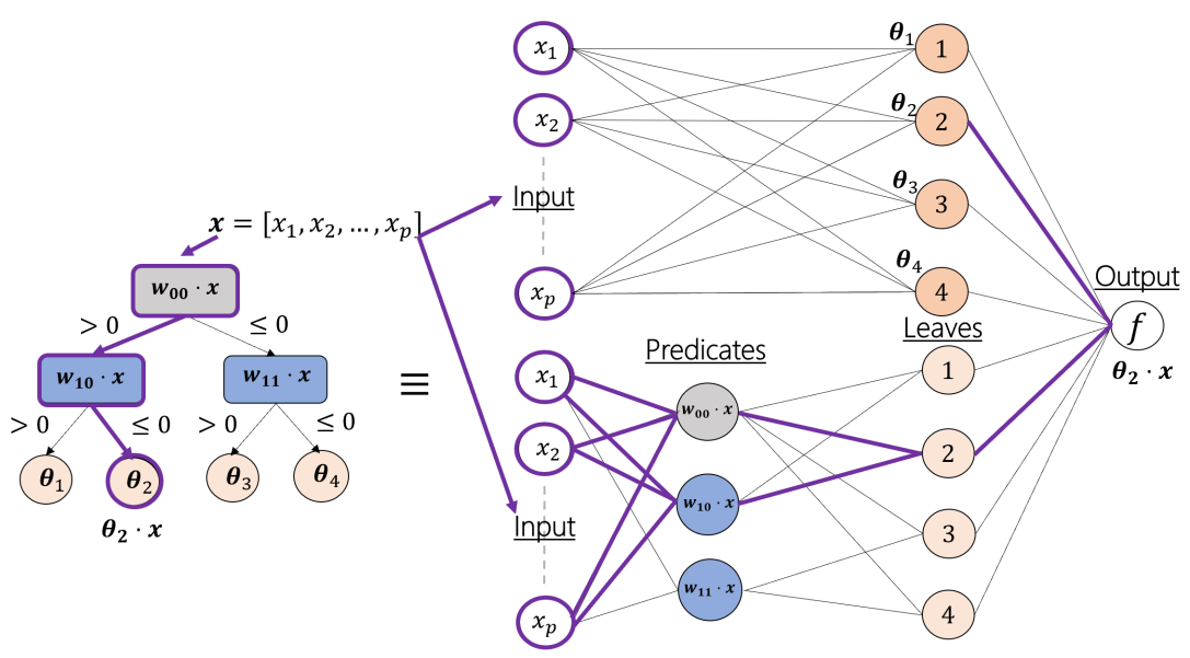
Figure 12. On the left is a decision tree of height 2. On the right is the equivalent EntropyNet with activation functions and weights as per the description in Definition 8. The path highlighted on the tree traversed by a given input example $\mathbf{x}$ has a one-to-one correspondence to a set of neurons that fire in the EntropyNet.

Next, we formally show that the EntropyNet architecture encodes the decision tree computation exactly.

Lemma 3 (Every Decision Tree is an EntropyNet).

For any given decision tree $f_{T}(.;\mathbf{W},\bm{\Theta})$ (in Definition 4), there is an EntropyNet architecture described in Definition 8 with a particular choice of model parameters, say $\widetilde{\mathbf{W}}$, that computes the same function as the tree. Let $f_{\emph{{Net}}}(.;\widetilde{\mathbf{W}})$ denote the function computed by the EntropyNet. We have,

$$f_{T}(\mathbf{x};\mathbf{W},\bm{\Theta})=f_{\emph{{Net}}}(\mathbf{x};\widetilde{\mathbf{W}}),\forall\mathbf{x}\in\mathbb{R}^{p}.$$

Not only is every decision tree encoded by some EntropyNet, but the vice versa also holds. Thus, the class of entropy nets and the class of decision trees (and therefore  Imp, from Lemmas 1 and 2) are identical.

Lemma 4 (Every EntropyNet is a Decision Tree).

For every neural network with 3 layers, with constraints on the weights and activations as described in Definition 8, there is a corresponding decision tree which represents the same function.

A.1. Updating $f_{\emph{{Net}}}$ model

Computing the gradient in the update Step 5 of Algorithm 4, with $f_{\emph{{Net}}}$ in lieu of $f$ given the equivalence above, and ensuring that the updates maintain a valid decision tree, is still challenging for the following reasons.

1. The activation function in the first (predicate) layer given in Definition 8 (1) is the sign function, which is discontinuous and non-differentiable. We need a relaxation of the activation function to allow learning.

2. The structural constraints on the weights of the leaf neurons given in Definition 8 (2) impose that the weights be integral, and in particular, $\{1,-1\}$-valued (see Figure 12). This is an inviolable constraint, to ensure that the root-to-leaf paths are preserved in the learned neural network model.

3. Finally, we need only one of the leaf neurons to fire in the leaf layer – this is ensured in Definition 8 (3), by the activation that thresholds the output at $h$. This essentially implements the AND of the predicates, which theoretically holds only when we use sign function in the predicate layer. Thus this requirement is at odds with any relaxation that we might want to use to mitigate the first challenge.

We address these challenges as follows:
(I) First, we relax the sign function using a scaled sigmoid function as the activation function for the predicate layer. In particular, for appropriately chosen $s>0$, we define:

$$\sigma_{s}(a):=\frac{1}{1+\exp(-s\ .\ a)},~{}\text{and}$$

(7) $$z^{(1)}_{ij}=2\sigma_{s}(\langle\widetilde{\mathbf{w}}_{ij}^{(1)},\mathbf{x}\rangle+b_{ij})-1.$$

Note that for sufficiently large $s$, the above activation behaves like the sign function. In practice, selecting $s$ can be tricky. If we choose $s$ very large, then it will be hard for the optimization to proceed and it will likely get stuck in a poor solution. On the other hand, using a small $s$ will lead to violation of constraints as discussed in challenge (3) above.

Even though the optimization tends to converge to a good $\widetilde{\mathbf{W}}$ with a small $s$ (when the model is effectively a neural network), the resulting decision tree model $\mathbf{W},\bm{\Theta}$ after conversion can be quite poor. On the other hand, we also observe that it is important for $s$ to be not too large (when the model is effectively a decision tree), otherwise the optimization cannot proceed. This motivates us to devise a careful scheduling of choices of $s$ from smaller values to larger values, letting the activation function approach the sign function, moving gradually from the space of neural networks to decision trees in the process.

(II) Second, we satisfy the integral constraints on the weights of the leaf neurons by simply anchoring the weights during training. Note that the number of non-zero weights in the second layer of EntropyNet is only $h\ .2^{h}$, as against standard dense neural network which has $O(2^{2h})$ connections.

(III) The above two ideas by themselves still do not guarantee convergence of the optimization to a good decision tree solution. In fact, the third challenge remains unaddressed. In particular, when we start with a small $s$ in the sigmoid activation in the beginning of the training, there is no guarantee that any ReLU activated neuron in the third layer, given in Eqn. (6), will fire at all, if we set $\epsilon$ to be very small. On the other hand, if we set $\epsilon$ to be large, many neurons will fire, thus violating the basic property of a decision tree (each example traverses a unique root-to-leaf path). Therefore, we follow the opposite schedule for $\epsilon$; we start with a large $\epsilon$ ensuring that gradient information propagates through these neurons, and gradually decrease $\epsilon$.

Appendix B Proofs

B.1. Proof of Lemma 1

Consider the parse tree of a given decision function $f:\mathbb{R}^{p}\to\mathbb{R}^{m}$ shown below in Figure 13, denoted by $\mathcal{P}$, where each internal node in the tree corresponds to a non-terminal of type $E$ (expression) or $S$ (statement), and leaf nodes correspond to real numbers (i.e. choices for $W$ in the expansion of $E$). We start by constructing an equivalent parse tree $\mathcal{P}^{\prime}$ for $f$, by transforming $\mathcal{P}$ in way that ensures that the computational semantics of the program is preserved.

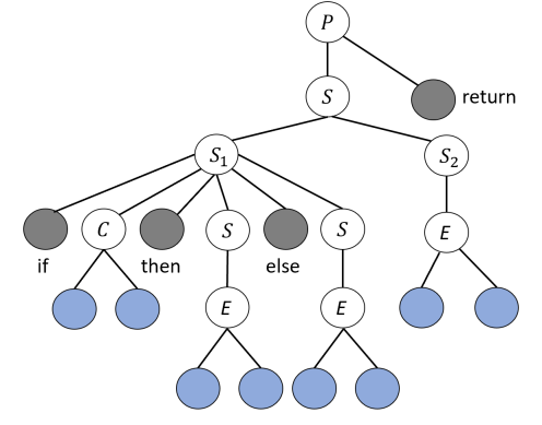
Figure 13. Parse tree for a decision function in Imp with $p=1$ (the blue terminal nodes correspond to choices for $W_{1}$ and $W_{2}$). The non-terminal $C$ is a short-hand for the conditional $E>0$.

The key transformation, called Expand, is as follows. For any internal node $S$ such that both of its children are of type $S$ (call them $S_{1}$ and $S_{2}$) (Figure 13 has one instance of this), let $\mathcal{P}_{S_{2}}$ denote the sub-tree of $\mathcal{P}$ rooted at $S_{2}$. Now, consider every root-to-leaf path in $\mathcal{P}_{S_{1}}$ starting from $S_{1}$ to the last internal node of type $S$. say $S^{\prime}$, along the path. We attach $\mathcal{P}_{S_{2}}$ as the second child of $S^{\prime}$ (note that $S^{\prime}$ has only child, because it is the last internal node). We now apply Expand to every such internal node $S$ such that both of its children are of type $S$. The resulting transformed parse tree $\mathcal{P}^{\prime}$ after applying Expand to the example in Figure 13 is shown in Figure 14.

Observe that $\mathcal{P}^{\prime}$ and $\mathcal{P}$ are equivalent, i.e. a) every assignment statement of type $o_{j}=E$ for some $1\leq j\leq m$ executed in $\mathcal{P}$, along any execution path of $f$, is also executed in $\mathcal{P}^{\prime}$, b) the order of the assignments is also identical (attaching as the right child in the above transform ensures this).

With this, we will now give a straight-forward construction of decision tree $f_{T}:\mathbb{R}^{p}\to\mathbb{R}^{m}$ (Definition 4) that computes the given decision function $f$. The root of the decision tree of $f_{T}$ corresponds to the first non-terminal $S$ in the parse-tree $\mathcal{P}^{\prime}$ (note that any program in Imp  has at least one non-terminal $S$ in its parse tree). For this single-node tree $f_{T}$ (as yet), initialize parameters $\bm{\Theta}=\{\bm{\theta}_{j}\}=\emptyset$. Now consider the sub-tree rooted at this $S$ in $\mathcal{P}^{\prime}$ referred to as $\mathcal{P}^{\prime}_{S}$. Note that there is no node in $\mathcal{P}^{\prime}$ both of whose children of type $S$. That leaves us with the following cases:

1. if the children node of $S$ in $\mathcal{P}^{\prime}_{S}$ correspond to if ($C$) then $S_{1}$ else $S_{2}$ then set the parameters $\mathbf{w}\in\mathbb{R}^{p+1}$ of the current root node of $f_{T}$ to the corresponding terminals in the conditional expression $C$. Then:
   a) create a left child to the current root in $f_{T}$, copy $\{\bm{\theta}_{j}\}$ of the current root node, make this the current root, and repeat step (1) with $S=S_{1}$.
   b) create a right child to the current root in $f_{T}$, copy $\{\bm{\theta}_{j}\}$ of the current root node, make this the current root, and repeat step (1) with $S=S_{2}$.

2. if the first (or only) child node of $S$ corresponds to assignment $o_{j}=E$, then set $\bm{\theta}_{j}\in\mathbb{R}^{p+1}$ of the current root node to the corresponding terminals in the expression $E$.

3. if the other child node of $S$ exists and is of type $S$ (call it $S^{\prime}$), then go to step (1) with $S=S^{\prime}$.

The height of the resulting tree $f_{T}$, say $h$, is proportional to the number of $S$ nodes in $\mathcal{P}^{\prime}$ that expand to a conditional statement (note that the height of the tree grows only in step (1) above). The size of $f_{T}$ is exponential in $h$.

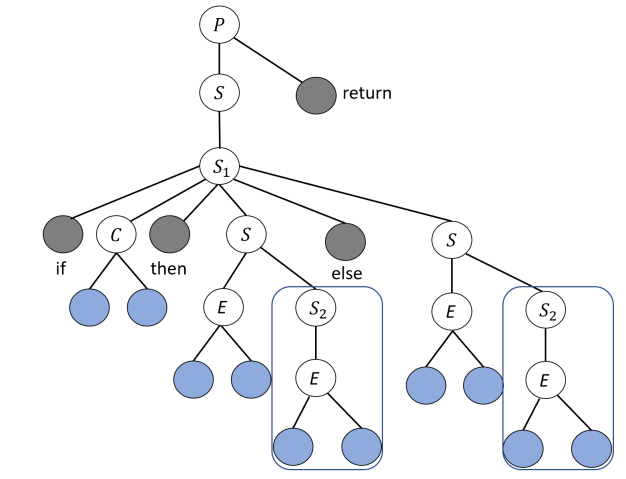
Figure 14. Applying Expand transform to the parse tree in Figure 13.

B.2. Proof of Lemma 2

This direction is straight-forward. We can synthesize the desired $f\in~{}\textsc{Imp}$ by doing a pre-order traversal of $f_{T}$. When we visit a leaf node, all the assignment statements of the form $o_{j}=E$ for $1\leq j\leq m$ will be synthesized corresponding to $\{\bm{\theta}_{j}\}$ parameters of the node.

B.3. Proof of Theorem 1

We refer the reader to the proof of Theorem 3.3 of Flaxman et al. (2005). Note that $n$ in their notation is the same as $T$ in ours.

B.4. Proof of Theorem 2

We appeal to the result in Corollary 2 of Shamir (2017), that uses the two-point gradient estimator given in (2), and matches the setting in our algorithm.

B.5. Proof of Theorem 3

We start by recalling a key lemma of (Flaxman et al., 2005) that uses the online gradient descent analysis by (Zinkevich, 2003) with unbiased random gradient estimates. We restate the result below for clarity, for the case when the reward is concave (the original result is stated for loss being convex). Let $\mathcal{B}_{d}(R)$ denote ball of radius $R$ in $\mathbb{R}^{d}$, and $\Pi_{S}(\mathbf{w})=\arg\min_{\mathbf{w}^{\prime}\in S}\|\mathbf{w}-\mathbf{w}^{\prime}\|$.

Lemma 5 (Lemma $3.1$, (Flaxman et al., 2005)).

Let $S\subset\mathcal{B}_{d}(R)\subset\mathbb{R}^{d}$ be a convex set, $c_{1},c_{2},\dots,c_{T}:S\mapsto\mathbb{R}$ be a sequence of concave, differentiable functions. Let $\mathbf{w}^{(1)},\mathbf{w}^{(2)},\dots,\mathbf{w}^{(T)}\in S$ be a sequence of predictions defined as $\mathbf{w}^{(1)}=0$ and $\mathbf{w}^{(t+1)}=\Pi_{S}(\mathbf{w}^{(t)}-\eta h^{(t)})$, where $\eta>0$, and $h^{(1)},h^{(2)},\dots,h^{(T)}$ are random variables such that $\mathbb{E}[h^{(t)}\big{|}\mathbf{w}^{(t)}]=c_{t}(\mathbf{w}^{(t)})$, and $\|h^{(t)}\|_{2}\leq G$, for some $G>0$ then, for $\eta=\frac{R}{G\sqrt{T}}$, the expected regret incurred by above prediction sequence is:

$$\max_{\mathbf{w}\in S}\sum_{t=1}^{T}c_{t}(\mathbf{w})-\mathbb{E}\bigg{[}\sum_{t=1}^{T}c_{t}(\mathbf{w}^{(t)})\bigg{]}\leq RG\sqrt{T}.$$

We need the following assumptions:
(1) reward function $r$ is bounded, i.e. $r:\mathbb{R}^{m}\mapsto[-C,C]$, for some numerical constant $C$.
(2) $r$ is concave in $\mathbf{w}\in\mathbb{R}^{m\times p}$ (note that $r(\mathbf{a})=r(\mathbf{w}\mathbf{x})$, where $\mathbf{w}\in\mathbb{R}^{m\times p}$ and $\mathbf{x}\in\mathbb{R}^{p}$).
(3) $\max_{t}\|\mathbf{x}^{(t)}\|_{2}\leq D$.

In the following, we will use the short-cut $\mathbf{a}=f(\mathbf{x};\mathbf{w})=\mathbf{w}\mathbf{x}$ and $\mathbf{a}^{(t)}=f(\mathbf{x}^{(t)};\mathbf{w}^{(t)})=\mathbf{w}^{(t)}\mathbf{x}^{(t)}$.

Also, in Algorithm 3, we work with parameters $\mathbf{w}\in\mathcal{W}=\mathcal{B}_{d}(mW)$, for some, possibly large number, $W$.

Let $\mathbf{U}$ denote the uniform distribution and $\mathcal{S}_{m}(1)$ denote the sphere in $\mathbb{R}^{m}$ of radius $1$. Now, define $\hat{r}:\mathbb{R}^{m}\mapsto[-C,C]$ such that $\hat{r}(\mathbf{a})=\mathbb{E}_{\mathbf{u}\sim\mathbf{U}(\mathcal{S}_{m}(1))}\big{[}r(\mathbf{a}+\delta\mathbf{u})\big{]}$, for any $\mathbf{a}\in\mathbb{R}^{m}$. Then applying the above Lemma 5 in the setting of Algorithm 3, on the concave function $\hat{r}$, with $h^{(t)}=\frac{m}{\delta}\big{(}r(\mathbf{a}^{(t)})\mathbf{u}\big{)}(\mathbf{x}^{(t)})^{\text{T}}$, and $\mathbf{u}\sim\mathbf{U}(\mathcal{S}_{m}(1))$ (note that this implies $\mathbb{E}[h^{(t)}\big{|}\mathbf{w}^{(t)}]=\nabla_{\mathbf{w}}\mathbb{E}_{\mathbf{u}}\big{[}r(\mathbf{a}^{(t)}+\delta\mathbf{u})\big{]}$, which can be seen from Lemma 2.1 of (Flaxman et al., 2005)), we get:

(8) $$\max_{\mathbf{w}\in\mathcal{W}}\sum_{t=1}^{T}\hat{r}(\mathbf{a})-\mathbb{E}\bigg{[}\sum_{t=1}^{T}\hat{r}(\mathbf{a}^{(t)})\bigg{]}\leq\frac{m^{2}WDC\sqrt{T}}{\delta},$$

as $\hat{r}(\cdot)$ is concave (in argument $\mathbf{w}\in\mathbb{R}^{m\times p}$) due to the assumption $(ii)$ above, and in this case $R\leq W$, and $\|h^{(t)}\|=\|\frac{m}{\delta}\big{(}{r(\mathbf{a}^{(t)})}\mathbf{u}\big{)}(\mathbf{x}^{(t)})^{\text{T}}\|\leq\frac{mDC}{\delta}$, so $G=\frac{mDC}{\delta}$ and hence we need to choose $\eta=\frac{W\delta}{DC\sqrt{T}}$.

Further since $r(\cdot)$ is assumed to be $L$-Lipschitz continuous (Definition 7), it follows from (8) that,

$$\max_{\mathbf{w}\in\mathcal{W}}\sum_{t=1}^{T}\big{(}r(\mathbf{a})-\delta L\big{)}-\mathbb{E}\bigg{[}\sum_{t=1}^{T}\big{(}r(\mathbf{a}^{(t)})+\delta L\big{)}\bigg{]}\leq\frac{m^{2}WDC\sqrt{T}}{\delta},$$

$$\implies \max_{\mathbf{w}\in\mathcal{W}}\sum_{t=1}^{T}r(\mathbf{a})-\mathbb{E}\bigg{[}\sum_{t=1}^{T}r(\mathbf{a}^{(t)})\bigg{]}\leq\frac{m^{2}WDC\sqrt{T}}{\delta}+2\delta LT$$

We want to minimize the RHS above with respect to $\delta$, which can be achieved by setting $\delta=m\Big{(}\frac{WDC}{2L\sqrt{T}}\Big{)}^{1/2}$. This finally gives:

$$R_{T}=\max_{\mathbf{w}\in\mathcal{W}}\frac{1}{T}\sum_{t=1}^{T}r(\mathbf{a})-\frac{1}{T}\mathbb{E}\bigg{[}\sum_{t=1}^{T}r(\mathbf{a}^{(t)})\bigg{]}\leq\frac{2m\sqrt{2WLDC}}{T^{1/4}},$$

which concludes the proof.

B.6. Proof of Lemma 3

In the EntropyNet architecture described in Definition 8, consider the path function $\mathbbm{1}_{\ell}$ and $g_{ij}$ corresponding to the given decision tree. For $i\in\{0,1,\dots,h-1\},j\in\{0,1,\dots,2^{i}-1\}$, set the predicate layer weights (Definition 8 (1)) as follows.

$$\widetilde{\mathbf{w}}^{(1)}_{ij}=\mathbf{w}_{ij},$$

where $\mathbf{w}_{ij}$ are the weights of the internal nodes of the given tree. In the activation function, choose $b_{ij}$ to be the corresponding biases of the nodes $\forall i,j$. Set the weights of the second set of neurons in the leaf layer (2) to the linear models in the tree:

$$\widetilde{\mathbf{w}}^{(2,2)}_{j}=\bm{\theta}_{j},$$

where $\bm{\theta}_{k}\in\mathbb{R}^{p}$ are the linear model coefficients in the $k$th leaf node; in the activation function, choose $b^{\prime}_{k}$ to be the bias in the corresponding linear model. By construction, the resulting $f_{\emph{{Net}}}$ computes the given tree function $f_{T}$, i.e. the weights chosen for the EntropyNet in the middle layer (Definition 8 (2 (a))) and the activation function ensure that for a path from root to some leaf node $j$, the one and only neuron that is activated (i.e. outputs $\epsilon$) in the leaf layer is the $j$th neuron (all other neurons output 0). The proof is complete.

B.7. Proof of Lemma 4

This holds by arguments similar to the proof of Lemma 3. The tree parameters corresponding to a given $f_{\emph{{Net}}}$ (and $h$ and $\epsilon$ in Definition 8) are precisely given in the following Algorithm 5. Note here $\mathbf{w}(p)$ denotes $p$th entry in the vector $\mathbf{w}$.

function InferTree($\widetilde{\mathbf{W}},h,\epsilon$)

1:     for $i\in\{0,1,\dots,h-1\}$ do // predicates at internal nodes $\mathbf{W}$

2:         for $j\in\{0,1,\dots,2^{i}-1\}$ do

3:              $\mathbf{w}_{ij}=[\widetilde{\mathbf{w}}^{(1)}_{ij}(0),\widetilde{\mathbf{w}}^{(1)}_{ij}(1),\dots,\widetilde{\mathbf{w}}^{(1)}_{ij}(p-1)]$

4:              $b_{ij}=\widetilde{\mathbf{w}}^{(1)}_{ij}(p)$               

5:     for $j\in\{0,1,\dots,2^{h}-1\}$ do // linear models at the leaves $\bm{\Theta}$

6:         $\bm{\theta}_{j}(k)=\widetilde{\mathbf{w}}^{(2,2)}_{j}(k)$, for $k\in\{0,1,\dots,p\}$

7:         $\bm{\theta}_{j}(p)=b^{\prime}_{j}$ (bias of the activation function, Definition 8 (2 b))      

8:     return $\mathbf{W}=\{\mathbf{w}_{ij},b_{ij}\},\bm{\Theta}=\{\bm{\theta}_{j}\}$

Algorithm 5 Inferring decision tree from EntropyNet

Appendix C Appendix to Section 5

C.1. PROSE details and additional results (for Section 5.2)

Here, we include additional results for the PROSE case study presented in the main text, Section 5.2, in Figures 16, 17 and 18. Figure 15 shows the FormatDateTimeRange heuristic that is part of $\mathsf{PROSE}$ (PROSE, 2015; Natarajan et al., 2019), with parameters of interest highlighted.

⬇

double FormatDateTimeRange(double base_SeparatorIsCommonDateTimeSeparator, ...) {

return -0.25*base_SeparatorIsCommonDateTimeSeparator +

0.07*base_SeparatorIsOnlySymbolsAndPunctuation +

-0.52*base_SeparatorIsOnlyWhitespace +

-0.12*base_SeparatorIsWrappedByWhitespace +

0.06*bias_FormatDateTimeRange +

1*score_FormatDateTimeRange_dtRoundingSpec +

1*score_FormatDateTimeRange_dtRoundingSpec2 +

1*score_FormatDateTimeRange_inputDateTime +

1*score_FormatDateTimeRange_outputDtFormat +

1*score_FormatDateTimeRange_s;

}

Figure 15. The FormatDateTimeRange heuristic in $\mathsf{PROSE}$ (PROSE, 2015; Natarajan et al., 2019) with parameters of interest highlighted.

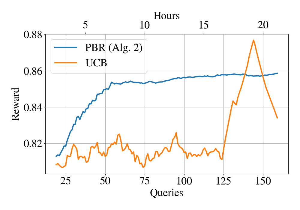
Figure 16. For the same setting as Figure 7, rewards obtained by $\mathsf{PBR}$ and UCB for tuning RegexPair with $3$ parameters (Figure 6); for the UCB algorithm, 3 parameters are discretized into $5*5*5=125$ actions.

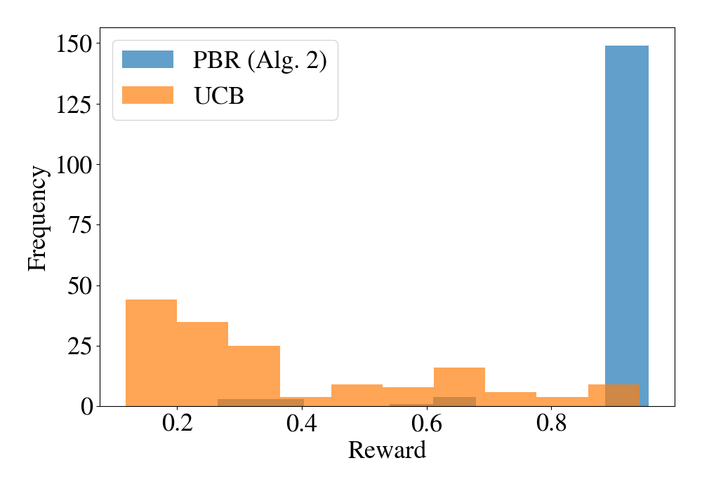
Figure 18. Distribution of rewards received by $\mathsf{PBR}$ and UCB when tuning FormatDateTimeRange (Figure 15) parameters, corresponding to the result shown in Figure 7 (b).

C.2. Sketch details (for Section 5.3)

Example code for $\mathsf{Sketch}$ specification given as input to the tool (Bodik and Solar-Lezama, 2006) is shown in Figure 19. We vary n, d, features, w_opt values in this code to produce the results presented in Section 5.3.

Relaxing Sketch specification. We know that there is a solution to problem (4) that achieves the objective value of 0. But, in some cases, it is still useful to fill the holes with values that yield a small enough objective value “close to” the optimal — i.e. fill the holes $\mathbf{w}$ so that $L(\mathbf{w})\leq L(\mathbf{w}^{*})+\epsilon=\epsilon$, where $L(\mathbf{w}):=\mathbb{E}[r\big{(}\mathbf{w}\cdot\mathbf{x}\big{)}]$. Thus we could relax the sketch specification, i.e. last line 5 of Figure 19, to assert (w[0] <= 10) & (w[1] <= 10) & (losses <= epsilon). As we increase $\epsilon$ away from 0, the search problem becomes easier, and therefore one expects to find some feasible solution, though it need not be optimal. Unfortunately, this intuition doesn’t hold for sketching — in some cases, it makes the computation even longer, because it takes more bits to encode the slackness constraint and ends up increasing the problem complexity. On the other hand, the algorithms used by $\mathsf{PBR}$ can yield a solution, close to the optimal, that improves with the time budget.

⬇

int sqloss (int score1, int score2) {

return (score1 - score2) * (score1 - score2);

}

int absloss (int score1, int score2) {

return score1 > score2 ? score1 - score2:

score2 - score1;

}

harness void paramSketch () {

int n = 2;

int d = 2;

int[n][d] features = {{-2,3}, {-3,-1}};

int[d] w_opt = {1,2};

int[d] w;

int losses = 0;

int[n] y;

for (int i=0; i < n; i++) {

y[i] = 0;

for (int j=0; j < d; j++) {

y[i] += w_opt[j] * features[i][j];

}

}

w[0] = ??;

w[1] = ??;

for (int i=0; i < n; i++) {

int score = 0;

for (int j=0; j < d; j++) {

score += w[j] * features[i][j];

}

losses += absloss(score, y[i]);

}

minimize (losses);

assert (w[0] <= 10) & (w[1] <= 10) & (losses == 0);

}

Figure 19. Example implementation of a sketch problem given to the $\mathsf{Sketch}$ tool (Bodik and Solar-Lezama, 2006) discussed in Section 5.3. Here, number of examples $n=2$ and number of holes to fill is $d=2$. The values for features are random integers sampled from the range [-10,10], and those for w_opt are random integers sampled from the range [0,10].

C.3. Fermat sketch (for Section 5.3)

In Section 5.3 (Figure 9) we have given the Thermostat sketch; Figure 20 shows the Aircraft sketch, the other function sketch discussed in Section 5.3. Both of the sketches originate from Chaudhuri et al. (2014), where they are also explained in more detail.

⬇

1double Aircraft(double v1, double v2) {

2 $\dots$

3 double criticalDist = ??(6, 9);

4 double safetyDist = 3.0;

5 double delay = ??(10, 15);

6 double delay2 = ??(9, 14);

7 assert(delay > 0.0; $\theta$);

8 assert(delay2 > 0.0; $\theta$);

9 assert(criticalDist > safetyDisty; $\theta$);

10 assert(criticalDist < 10; $\theta$);

11 for (int i=0; i<50; i=i+1) {

12 if (stage == CRUISE) {

13 move_straight(x1, y1, x2, y2, v1, v2);

14 if ($\delta$(x1, y1, x2, y2) < criticalDist) {

15 stage = LEFT;

16 assert(!haveLooped; $\theta$);

17 steps = 0;

18 }

19 }

20 if (stage == LEFT) {

21 move_left(x1, y1, x2, y2, v1, v2);

22 steps = steps + 1;

23 if (delay - steps < 0) {

24 stage = STRAIGHT;

25 steps = 0;

26 }

27 }

28 if (stage == STRAIGHT) {

29 move_straight(x1, y1, x2, y2, v1, v2);

30 steps = steps + 1;

31 if (delay - steps < 0) {

32 stage = RIGHT;

33 steps = 0;

34 }

35 }

36 if (stage == RIGHT) {

37 move_right(x1, y1, x2, y2, v1, v2);

38 steps = steps + 1;

39 if (delay - steps < 0) {

40 stage = CRUISE;

41 haveLooped = true;

42 }

43 }

44 assert($\delta$(x1, y1, x2, y2) < safetyDist; $\theta$);

45 }

46 return 2 * delay + delay2;

47}

Figure 20. Aircraft sketch (Chaudhuri et al., 2014).

C.4. Decision tree problems Xor and Slates (for Section 5.4)

The Xor problem instance discussed in the main paper is presented in Figure 21. Slates is a more complex hypothetical tuning problem, where we wish to learn a piece-wise constant threshold function based on the values of 2 features, to decide what the threshold for the input should be (these type of heuristics are common in systems); here, we have 6 different possible thresholds that depend on the 2 features as shown in Figure 22. The decision functions learnt by our Algorithm 4 for the Xor and the Slates problem instances are given in Figures 23 and 24.

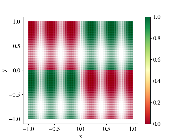
Figure 21. (Xor problem) Expected values as a function of the two features x and y is given by the XOR function, that can be modeled by a tree of height 2. Best viewed in color.

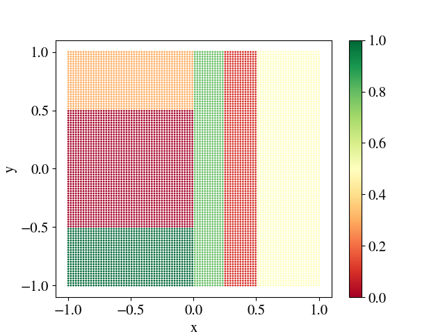
Figure 22. (Slates problem) Expected values (thresholds) as a function of the two features x and y is given by a piece-wise constant function, that can be modeled by a tree of height 3. Best viewed in color.

⬇

double XOR(double x1, double x2)

{

if (x2 <= -0.02)

if (x1 >= 0.04)

return 0;

else return 1;

else

if (x1 <= (-0.01 * x2 - 0.03))

return 0.03;

else return 0.98;

}

Figure 23. The tree heuristic learnt by $\mathsf{PBR}$ for the Xor problem in Figure 21.

⬇

double ThresholdMap(double x, double y) {

if (x >= -0.01*y)

if (x >= 0.25)

if (x >= 0.41) return 0.5;

else return 0.1;

else

return 0.81;

else

if (y >= -0.01*x - 0.41)

if (y >= 0.01*x + 0.43) return 0.3;

else return 0;

else

if (0.94*x >= 0.34*y + 2.58) return 0.47;

else return 1;

}

Figure 24. The tree heuristic learnt by $\mathsf{PBR}$ for deciding the threshold parameter described in Figure 22.

Appendix D Appendix: $\mathsf{PBR}$ Specification API

Here we give the details of the API we have built for developers to use $\mathsf{PBR}$ and our algorithms.
1. Creation. The Create API creates an instance of the synthesis/parameter learning problem for $\mathsf{PBR}$. This API allows several optional arguments that essentially helps the programmer encode domain knowledge for the problem:
(a) the name of the decision function to learn,
(b) optional features, which the programmer uses to model the decision as a function of the context,
(c) the model type (“template”) for computing decisions, as a function of feature values and parameter values (we currently support constant or linear model or decision tree as discussed in the main paper),
(d) optional initial values for the parameters, set to 0 by default
(e) optional constraints on the parameters to be tuned; the API supports range constraints (min and max), and type constraints (e.g., isInt is True if the parameters takes only integral values).

Constraints( double min, double max, bool isInt)

int Create( string param,

           double initValue = 0,

           Dictionary< string, Constraints> constraints = null,

           string[] features = null,

           enum template)

2. Connection. The Create API sets up a data store instance in the back-end for tuning the specified parameters, initializes the necessary background services to maintain/update this store. A unique identifier to this store instance is returned by the call to Create. The next step is to connect the client to this instance. The Connect API connects a parameter learning instance to a $\mathsf{PBR}$ object.

void Connect ( int problemId)
Note that if a store already exists (for the parameter(s) of interest), then the client can directly connect to the instance by referencing the unique identifier to the instance, because store instances are persistent. This also enables multiple clients (distributed spatially and/or temporally) to query the latest decisions for as well as give feedback to the same learning problem. The creation of a store instance can also be performed through a separate GUI or a plugin.

3. Prediction. This interface encapsulates PBR.DecisionFunction introduced in Example 2.1. With the Predict interface, the programmer can query the decision outcome using the learnt model. It takes the feature values as input from the context and returns the decision outcome:

(int, double) Predict ( Dictionary< string, double> features)

Internally, it works by (1) retrieving the current version of the learnt model and parameters as an expression tree, (2) converting the expression tree into a lambda expression, and (3) running the lambda expression using the given feature values as arguments. The lambda expression is cached in the client as as to perform further predictions without needing to contact the server. If the model is refreshed, then the cache is cleared in the client, and the subsequent call to Predict retrieves the updated expression from the model and recomputes the corresponding lambda expression. Note that Predict returns a pair of values – a unique identifier which identifies the particular invocation of Predict, and the predicted decision value.

If the client wishes to retrieve the expression tree to inspect the learnt model, it can use the GetExprTree API:

Expression<TDelegate> GetExprTree ( Dictionary< string, double> features)
4. Reward. This is the PBR.AssignReward interface introduced in Example 2.1, which allows the client to specify a reward and also associate it with a particular invocation of Predict (the default is the last invocation, as in Figure 3).

void AssignReward( int invocationId, double reward)
We note that a decision is associated with many parameters (from a linear model or decision tree) and the reward specified is associated with all of these parameter choices (see Figure 5). This aspect of $\mathsf{PBR}$ distinguishes it from other solutions like Decision Service (Agarwal et al., 2016) and $\mathsf{SmartChoices}$ (Carbune et al., 2019); they rely on providing explicit reward for each parameter and decision value, whereas we do not require that disambiguation — our problem formulation and learning enables working with a single reward (i.e. value of the key system level metric) for a decision (and can be generalized to set of decisions as well), and in turn tuning several parameters together.

5. Refresh. The Refresh API learns an updated model based on the data collected in the store instance, using the algorithms presented in Section 4: void Refresh()

The client can choose to perform either online learning or offline learning by how frequently it calls Refresh. Calling Refresh   say once a day, results in offline learning, and calling it every few minutes results in online learning. As a side-effect, Refresh clears the client side cache used by Predict, as discussed above.

References

- (1)
- Abadi et al. (2015) Martín Abadi, Ashish Agarwal, Paul Barham, Eugene Brevdo, Zhifeng Chen, Craig Citro, Greg S. Corrado, Andy Davis, Jeffrey Dean, Matthieu Devin, Sanjay Ghemawat, Ian Goodfellow, Andrew Harp, Geoffrey Irving, Michael Isard, Yangqing Jia, Rafal Jozefowicz, Lukasz Kaiser, Manjunath Kudlur, Josh Levenberg, Dandelion Mané, Rajat Monga, Sherry Moore, Derek Murray, Chris Olah, Mike Schuster, Jonathon Shlens, Benoit Steiner, Ilya Sutskever, Kunal Talwar, Paul Tucker, Vincent Vanhoucke, Vijay Vasudevan, Fernanda Viégas, Oriol Vinyals, Pete Warden, Martin Wattenberg, Martin Wicke, Yuan Yu, and Xiaoqiang Zheng. 2015. TensorFlow: Large-Scale Machine Learning on Heterogeneous Systems. https://www.tensorflow.org/
- Agarwal et al. (2016) Alekh Agarwal, Sarah Bird, Markus Cozowicz, Luong Hoang, John Langford, Stephen Lee, Jiaji Li, Dan Melamed, Gal Oshri, Oswaldo Ribas, et al. 2016. A multiworld testing decision service. arXiv preprint arXiv:1606.03966 7 (2016).
- Agarwal et al. (2019) Naman Agarwal, Alon Gonen, and Elad Hazan. 2019. Learning in Non-convex Games with an Optimization Oracle. In Conference on Learning Theory. 18–29.
- Bao et al. (2019) Liang Bao, Xin Liu, Fangzheng Wang, and Baoyin Fang. 2019. ACTGAN: automatic configuration tuning for software systems with generative adversarial networks. In 2019 34th IEEE/ACM International Conference on Automated Software Engineering (ASE). IEEE, 465–476.
- Besson (2018) Lilian Besson. 2018. SMPyBandits: an Open-Source Research Framework for Single and Multi-Players Multi-Arms Bandits (MAB) Algorithms in Python. Online at: github.com/SMPyBandits/SMPyBandits. https://github.com/SMPyBandits/SMPyBandits/ Code at https://github.com/SMPyBandits/SMPyBandits/, documentation at https://smpybandits.github.io/.
- Bietti et al. (2018) Alberto Bietti, Alekh Agarwal, and John Langford. 2018. A contextual bandit bake-off. arXiv preprint arXiv:1802.04064 (2018).
- Bodik and Solar-Lezama (2006) Ras Bodik and Armando Solar-Lezama. 2006. SKETCH synthesis tool (commitid: 26040ed). (2006). https://bitbucket.org/gatoatigrado/sketch-frontend/wiki/Home
- Bornholt et al. (2016) James Bornholt, Emina Torlak, Dan Grossman, and Luis Ceze. 2016. Optimizing synthesis with metasketches. In Proceedings of the 43rd Annual ACM SIGPLAN-SIGACT Symposium on Principles of Programming Languages. 775–788.
- Carbune et al. (2019) Victor Carbune, Thierry Coppey, Alexander Daryin, Thomas Deselaers, Nikhil Sarda, and Jay Yagnik. 2019. SmartChoices: Hybridizing Programming and Machine Learning. ICML Workshop RL4RealLife (2019).
- Carreira-Perpinán and Tavallali (2018) Miguel A Carreira-Perpinán and Pooya Tavallali. 2018. Alternating optimization of decision trees, with application to learning sparse oblique trees. In Advances in Neural Information Processing Systems. 1211–1221.
- Chaudhuri et al. (2014) Swarat Chaudhuri, Martin Clochard, and Armando Solar-Lezama. 2014. Bridging boolean and quantitative synthesis using smoothed proof search. In Proceedings of the 41st ACM SIGPLAN-SIGACT Symposium on Principles of Programming Languages. 207–220.
- Chaudhuri et al. (2012) Swarat Chaudhuri, Sumit Gulwani, and Roberto Lublinerman. 2012. Continuity and robustness of programs. Commun. ACM 55, 8 (2012), 107–115.
- Esmaeilzadeh et al. (2012) H. Esmaeilzadeh, A. Sampson, L. Ceze, and D. Burger. 2012. Neural Acceleration for General-Purpose Approximate Programs. In 2012 45th Annual IEEE/ACM International Symposium on Microarchitecture. 449–460.
- Flaxman et al. (2005) Abraham D Flaxman, Adam Tauman Kalai, and H Brendan McMahan. 2005. Online convex optimization in the bandit setting: gradient descent without a gradient. In Proceedings of the sixteenth annual ACM-SIAM Symposium on Discrete Algorithms. 385–394.
- Ghadimi and Lan (2013) Saeed Ghadimi and Guanghui Lan. 2013. Stochastic first-and zeroth-order methods for nonconvex stochastic programming. SIAM Journal on Optimization 23, 4 (2013), 2341–2368.
- Gulwani (2011) Sumit Gulwani. 2011. Automating string processing in spreadsheets using input-output examples. In ACM SIGPLAN Notices, Vol. 46. ACM, 317–330.
- Gulwani and Jain (2017) Sumit Gulwani and Prateek Jain. 2017. Programming by Examples: PL meets ML. In Asian Symposium on Programming Languages and Systems. Springer, 3–20.
- Gulwani et al. (2019) Sumit Gulwani, Kunal Pathak, Arjun Radhakrishna, Ashish Tiwari, and Abhishek Udupa. 2019. Quantitative Programming by Examples. arXiv preprint arXiv:1909.05964 (2019).
- Guo et al. (2018) Jianmei Guo, Dingyu Yang, Norbert Siegmund, Sven Apel, Atrisha Sarkar, Pavel Valov, Krzysztof Czarnecki, Andrzej Wasowski, and Huiqun Yu. 2018. Data-efficient performance learning for configurable systems. Empirical Software Engineering 23, 3 (2018), 1826–1867.
- Iyer et al. (2019) Arun Iyer, Manohar Jonnalagedda, Suresh Parthasarathy, Arjun Radhakrishna, and Sriram K Rajamani. 2019. Synthesis and machine learning for heterogeneous extraction. In Proceedings of the 40th ACM SIGPLAN Conference on Programming Language Design and Implementation. 301–315.
- Johari et al. (2017) Ramesh Johari, Pete Koomen, Leonid Pekelis, and David Walsh. 2017. Peeking at a/b tests: Why it matters, and what to do about it. In Proceedings of the 23rd ACM SIGKDD International Conference on Knowledge Discovery and Data Mining. 1517–1525.
- Kaltenecker et al. (2019) Christian Kaltenecker, Alexander Grebhahn, Norbert Siegmund, Jianmei Guo, and Sven Apel. 2019. Distance-based sampling of software configuration spaces. In 2019 IEEE/ACM 41st International Conference on Software Engineering (ICSE). IEEE, 1084–1094.
- Kohavi and Longbotham (2017) Ron Kohavi and Roger Longbotham. 2017. Online Controlled Experiments and A/B Testing. Encyclopedia of machine learning and data mining 7, 8 (2017), 922–929.
- Krishnamurthy et al. (2019) Akshay Krishnamurthy, John Langford, Aleksandrs Slivkins, and Chicheng Zhang. 2019. Contextual bandits with continuous actions: Smoothing, zooming, and adapting. In Conference on Learning Theory. 2025–2027.
- Le et al. (2017) Xuan-Bach D Le, Duc-Hiep Chu, David Lo, Claire Le Goues, and Willem Visser. 2017. S3: syntax-and semantic-guided repair synthesis via programming by examples. In Proceedings of the 2017 11th Joint Meeting on Foundations of Software Engineering. ACM, 593–604.
- Liang et al. (2016) Jia Hui Liang, Vijay Ganesh, Krzysztof Czarnecki, and Pascal Poupart. 2016. MapleGlucose and MapleCMS. SAT COMPETITION 2016 (2016), 50.
- Natarajan et al. (2019) Nagarajan Natarajan, Danny Simmons, Naren Datha, Prateek Jain, and Sumit Gulwani. 2019. Learning Natural Programs from a Few Examples in Real-Time. In Proceedings of Machine Learning Research (Proceedings of Machine Learning Research), Kamalika Chaudhuri and Masashi Sugiyama (Eds.), Vol. 89. PMLR, 1714–1722. http://proceedings.mlr.press/v89/natarajan19a.html
- Norouzi et al. (2015) Mohammad Norouzi, Maxwell Collins, Matthew A Johnson, David J Fleet, and Pushmeet Kohli. 2015. Efficient non-greedy optimization of decision trees. In Advances in Neural Information Processing Systems. 1729–1737.
- Padhi et al. (2017) Saswat Padhi, Prateek Jain, Daniel Perelman, Oleksandr Polozov, Sumit Gulwani, and Todd Millstein. 2017. FlashProfile: Interactive Synthesis of Syntactic Profiles. arXiv preprint arXiv:1709.05725 (2017).
- PCWorld (2012) PCWorld. 2012. Microsoft Office 2013 Preview: Hands On. https://www.pcworld.com/article/259260/microsoft_office_2013_customer_preview_first_impressions.html
- Polozov and Gulwani (2015) Oleksandr Polozov and Sumit Gulwani. 2015. Flashmeta: A framework for inductive program synthesis. ACM SIGPLAN Notices 50, 10 (2015), 107–126.
- PROSE (2015) PROSE. 2015. Program synthesis from input-output examples (PROSE). Microsoft SDK (2015). https://microsoft.github.io/prose
- Rapin and Teytaud (2018) J. Rapin and O. Teytaud. 2018. Nevergrad - A gradient-free optimization platform. https://GitHub.com/FacebookResearch/Nevergrad.
- Raza and Gulwani (2018) Mohammad Raza and Sumit Gulwani. 2018. Disjunctive Program Synthesis: a Robust Approach to Programming by Example. Appearing in AAAI (2018).
- Rolim et al. (2017) Reudismam Rolim, Gustavo Soares, Loris D’Antoni, Oleksandr Polozov, Sumit Gulwani, Rohit Gheyi, Ryo Suzuki, and Björn Hartmann. 2017. Learning syntactic program transformations from examples. In Proceedings of the 39th International Conference on Software Engineering. IEEE Press, 404–415.
- Sayyad et al. (2013) Abdel Salam Sayyad, Joseph Ingram, Tim Menzies, and Hany Ammar. 2013. Scalable product line configuration: A straw to break the camel’s back. In 2013 28th IEEE/ACM International Conference on Automated Software Engineering (ASE). IEEE, 465–474.
- Sethi (1990) Ishwar Krishnan Sethi. 1990. Entropy nets: from decision trees to neural networks. Proc. IEEE 78, 10 (1990), 1605–1613.
- Shamir (2017) Ohad Shamir. 2017. An optimal algorithm for bandit and zero-order convex optimization with two-point feedback. The Journal of Machine Learning Research 18, 1 (2017), 1703–1713.
- Siegmund et al. (2015) Norbert Siegmund, Alexander Grebhahn, Sven Apel, and Christian Kästner. 2015. Performance-influence models for highly configurable systems. In Proceedings of the 2015 10th Joint Meeting on Foundations of Software Engineering. 284–294.
- Solar-Lezama et al. (2006) Armando Solar-Lezama, Liviu Tancau, Rastislav Bodik, Sanjit Seshia, and Vijay Saraswat. 2006. Combinatorial sketching for finite programs. In Proceedings of the 12th international conference on Architectural support for programming languages and operating systems. 404–415.
- Sutton and Barto (2011) Richard S Sutton and Andrew G Barto. 2011. Reinforcement learning: An introduction. (2011).
- T. Cazenave (2019) J. Rapin O. Teytaud T. Cazenave, M. Oquab. 2019. Parallel Noisy Optimization in Front of Simulators: Optimism, Pessimism, Repetitions Population Control. In proceedings of CEC 2019 workshops. https://www.lamsade.dauphine.fr/~cazenave/papers/games_cec.pdf
- Verma et al. (2019) Abhinav Verma, Hoang Le, Yisong Yue, and Swarat Chaudhuri. 2019. Imitation-projected programmatic reinforcement learning. In Advances in Neural Information Processing Systems. 15752–15763.
- Verma et al. (2018) Abhinav Verma, Vijayaraghavan Murali, Rishabh Singh, Pushmeet Kohli, and Swarat Chaudhuri. 2018. Programmatically Interpretable Reinforcement Learning. In International Conference on Machine Learning. 5045–5054.
- Zinkevich (2003) Martin Zinkevich. 2003. Online convex programming and generalized infinitesimal gradient ascent. In Proceedings of the 20th international conference on machine learning (icml-03). 928–936.