Early stopping and polynomial smoothing in regression with reproducing kernels

Abstract

In this paper, we study the problem of early stopping for iterative learning algorithms in a reproducing kernel Hilbert space (RKHS) in the nonparametric regression framework. In particular, we work with the gradient descent and (iterative) kernel ridge regression algorithms. We present a data-driven rule to perform early stopping without a validation set that is based on the so-called minimum discrepancy principle. This method enjoys only one assumption on the regression function: it belongs to a reproducing kernel Hilbert space (RKHS). The proposed rule is proved to be minimax-optimal over different types of kernel spaces, including finite-rank and Sobolev smoothness classes. The proof is derived from the fixed-point analysis of the localized Rademacher complexities, which is a standard technique for obtaining optimal rates in the nonparametric regression literature. In addition to that, we present simulation results on artificial datasets that show the comparable performance of the designed rule with respect to other stopping rules such as the one determined by $V-$fold cross-validation.

1 Introduction

The present paper is concerned with nonparametric regression by means of a reproducing kernel Hilbert space (RKHS) associated with a reproducing kernel [Aro50, Wah90, SS01, Gu13]. There is a large amount of literature on the application of kernel machines in many areas of science and engineering [SS01, SC+04, Zha+07], which is out of the main scope of the paper.

A family of linear estimators called spectral filter estimators [EHN96, YRC07, BPR07, Bal+12] can be seen as particular instances of iterative learning algorithms. This family includes two famous examples: gradient descent and iterative (Tikhonov) ridge regression. In several papers, it was observed empirically and proved theoretically that these two algorithms are closely related [FP04, YRC07, RWY14, Ang+15, AZT18]. For example, [AZT18] showed that in the linear regression model under the calibration $t=1/\lambda$, where $t$ is the time parameter in gradient descent and $\lambda$ the tuning parameter in ridge regression, the risk error of gradient descent could not be much higher than that of ridge regression. This gives some intuition of why the idea of implicit regularization could work.

Early stopping rule (ESR) is a form of regularization based on choosing when to stop an iterative algorithm based on some design criterion. Its main idea is lowering the computational complexity of an iterative algorithm while preserving its statistical optimality. This approach is quite old and initially was developed for Landweber iterations to solve ill-posed matrix problems in the 1970s [Wah87, EHN96]. The next wave of interest in this topic was in the 1990s and has been applied to neural network parameters learning with (stochastic) gradient descent [Pre98, CLG01]. For instance, [Pre98] suggested some heuristics, that rely on monitoring at the same time the train and validation errors for stopping the learning process, and gave some consistent simulation findings. Nevertheless, until the 2000s, there was a lack of theoretical understanding of this phenomenon. Recent papers provided some insights for the connection between early stopping and boosting methods [BY03, ZY+05, BT07, WYW17], gradient descent, and Tikhonov regularization in a reproducing kernel Hilbert space (RKHS) [YRC07, BPR07, RWY14]. For instance, [BY03] established the first optimal in-sample convergence rate of $L^{2}$-boosting with early stopping. Raskutti et al. [RWY14] provided a result on a stopping rule that achieves the minimax-optimal rate for kernelized gradient descent and ridge regression over different smoothness classes. This work established an important connection between the localized Radamacher complexities [BBM+05, Kol+06, Wai19], that characterizes the size of the explored function space, and early stopping. The main drawback of the result is that one needs to know the RKHS-norm of the regression function or its tight upper bound in order to apply this early stopping rule in practice. Besides that, this rule is design-dependent, which limits its practical application as well. In the subsequent work, [WYW17] showed how to control early stopping optimality via the localized Gaussian complexities in RKHS for different boosting algorithms ($L^{2}$-boosting, LogitBoost, and AdaBoost). Another theoretical result for a not data-driven ESR was built by [BK16], where the authors proved a minimax-optimal (in the ${L}_{2}(\mathbb{P}_{X})$ out-of-sample norm) stopping rule for conjugate gradient descent in the nonparametric regression setting. [Ang+15] proposed a different approach, where the authors focused on both time/memory computational savings combining early stopping with Nystrom subsampling technique.

Some stopping rules, that (potentially) could be applied in practice, were provided by [BHR16, BHR+18] and [Sta19], and were based on the so-called minimum discrepancy principle [EHN96, Han10, BM12, BK16]. This principle consists of monitoring the empirical risk and determining the first iteration at which a given learning algorithm starts to fit the noise. In the papers mentioned, the authors considered spectral filter estimators such as gradient descent, Tikhonov (ridge) regularization, and spectral cut-off regression for the linear Gaussian sequence model, and derived several oracle-type inequalities for the proposed ESR. The main deficiency of the works [BHR16, BHR+18, Sta19] is that the authors dealt only with the linear Gaussian sequence model, and the minimax optimality result was restricted to the spectral cut-off estimator. It is worth to mention that [Sta19] introduced the so-called polynomial smoothing strategy to achieve optimality of the minimum discrepancy principle ESR over Sobolev balls for the spectral cut-off estimator. More recently, [CW20] studied a minimum discrepancy principle stopping rule and its modified (they called it smoothed as well) version, where they provided the range of values of the regression function regularity, for which these stopping rules are optimal for different spectral filter estimators in RKHS.

Contribution. Hence, to the best of our knowledge, there is no fully data-driven stopping rule for gradient descent or ridge regression in RKHS that does not use a validation set, does not depend on the parameters of the model such as the RKHS-norm of the regression function, and explains why it is statistically optimal. In our paper, we combine techniques from [RWY14], [BHR16], and [Sta19] to construct such an ESR. Our analysis is based on the bias and variance trade-off of an estimator, and we try to catch the iteration of their intersection by means of the minimum discrepancy principle [BM12, BHR16, CW20] and the localized Rademacher complexities [Men02, BBM+05, Kol+06, Wai19]. In particular, for the kernels with infinite rank, we propose to use a special technique [BM12, Sta19] for the empirical risk in order to reduce its variance. Further, we introduce new notions of smoothed empirical Rademacher complexity and smoothed critical radius to achieve minimax optimality bounds for the functional estimator based on the proposed rule. This can be done by solving the associated fixed-point equation. It implies that the bounds in our analysis cannot be improved (up to numeric constants). It is important to note that in the present paper, we establish an important connection between a smoothed version of the statistical dimension of $n$-dimensional kernel matrix, introduced by [YPW17] for randomized projections in kernel ridge regression, with early stopping (see Section 4.3 for more details). We show also how to estimate the variance $\sigma^{2}$ of the model, specifically, for the class of polynomial eigenvalue decay kernels. In the meanwhile, we provide experimental results on artificial data indicating the consistent performance of the proposed rules.

Outline of the paper. The organization of the paper is as follows. In Section 2, we introduce the background on nonparametric regression and reproducing kernel Hilbert space. There, we explain the updates of two spectral filter iterative algorithms: gradient descent and (iterative) kernel ridge regression, that will be studied. In Section 3, we clarify how to compute our first early stopping rule for finite-rank kernels and provide an oracle-type inequality (Theorem 3.1) and an upper bound for the risk error of this stopping rule with fixed covariates (Corollary 3.2). After that, we present a similar upper bound for the risk error with random covariates (Theorem 3.4) that is proved to be minimax-rate optimal. By contrast, Section 4 is devoted to the development of a new stopping rule for infinite-rank kernels based on the polynomial smoothing [BM12, Sta19] strategy. There, Theorem 4.1 shows, under some quite general assumptions on the eigenvalues of the kernel matrix, a high probability upper bound for the performance of this stopping rule measured in the $L_{2}(\mathbb{P}_{n})$ in-sample norm. In particular, this upper bound leads to minimax optimality over Sobolev smoothness classes. In Section 5, we compare our stopping rules to other rules, such as methods using hold-out data and $V-$fold cross-validation. After that, we propose using a strategy for the estimation of the variance $\sigma^{2}$ of the regression model. Section 6 summarizes the content of the paper and describes some perspectives. Supplementary and more technical proofs are deferred to Appendix.

2 Nonparametric regression and reproducing kernel framework

2.1 Probabilistic model and notation

The context of the present work is that of nonparametric regression, where an i.i.d. sample $\{(x_{i},y_{i}),\ i=1,\ldots,n\}$ of cardinality $n$ is given, with $x_{i}\in\mathcal{X}\ (\textnormal{feature space})$ and $\ y_{i}\in\mathbb{R}$. The goal is to estimate the regression function $f^{*}:\mathcal{X}\to\mathbb{R}$ from the model

$$y_{i}=f^{*}(x_{i})+\overline{\varepsilon}_{i},\qquad i=1,\ldots,n,$$ (1)

where the error variables $\overline{\varepsilon}_{i}$ are i.i.d. zero-mean Gaussian random variables $\mathcal{N}(0,\sigma^{2})$, with $\sigma>0$. In all what follows (except for Section 5, where results of empirical experiments are reported), the values of $\sigma^{2}$ is assumed to be known as in [RWY14] and [WYW17].

Along the paper, calculations are mainly derived in the fixed-design context, where the $\{x_{i}\}_{i=1}^{n}$ are assumed to be fixed, and only the error variables $\{\overline{\varepsilon}_{i}\}_{i=1}^{n}$ are random. In this context, the performance of any estimator $\widehat{f}$ of the regression function $f^{*}$ is measured in terms of the so-called empirical norm, that is, the $L_{2}(\mathbb{P}_{n})$-norm defined by

$$\lVert\widehat{f}-f^{*}\rVert_{n}^{2}\coloneqq\frac{1}{n}\sum_{i=1}^{n}\Big{[}\widehat{f}(x_{i})-f^{*}(x_{i})\Big{]}^{2},$$

where $\lVert h\rVert_{n}\coloneqq\sqrt{1/n\sum_{i=1}^{n}h(x_{i})^{2}}$ for any bounded function $h$ over $\mathcal{X}$, and $\langle\cdot,\cdot\rangle_{n}$ denotes the related inner-product defined by $\langle h_{1},h_{2}\rangle_{n}\coloneqq 1/n\sum_{i=1}^{n}h_{1}(x_{i})h_{2}(x_{i})$ for any functions $h_{1}$ and $h_{2}$ bounded over $\mathcal{X}$. In this context, $\mathbb{P}_{\varepsilon}$ and $\mathbb{E}_{\varepsilon}$ denote the probability and expectation, respectively, with respect to the $\{\overline{\varepsilon}_{i}\}_{i=1}^{n}$.

By contrast, Section 3.1.2 discusses some extensions of the previous results to the random design context, where both the covariates $\{x_{i}\}_{i=1}^{n}$ and the responses $\{y_{i}\}_{i=1}^{n}$ are random variables. In this random design context, the performance of an estimator $\widehat{f}$ of $f^{*}$ is measured in terms of the $L_{2}(\mathbb{P}_{X})$-norm defined by

$$\lVert\widehat{f}-f^{*}\rVert_{2}^{2}\coloneqq\mathbb{E}_{X}\Big{[}(\widehat{f}(X)-f^{*}(X))^{2}\Big{]},$$

where $\mathbb{P}_{X}$ denotes the probability distribution of the $\{x_{i}\}_{i=1}^{n}$. In what follows, $\mathbb{P}$ and $\mathbb{E}$, respectively, state for the probability and expectation with respect to the couples $\{(x_{i},y_{i})\}_{i=1}^{n}$.

Notation.

Throughout the paper, $\lVert\cdot\rVert$ and $\langle\cdot,\cdot\rangle$ are the usual Euclidean norm and inner product in $\mathbb{R}^{n}$. We shall write $a_{n}\lesssim b_{n}$ whenever $a_{n}\leq Cb_{n}$ for some numeric constant $C>0$ for all $n\geq 1$. $a_{n}\gtrsim b_{n}$ whenever $a_{n}\geq Cb_{n}$ for some numeric constant $C>0$ for all $n\geq 1$. Similarly, $a_{n}\asymp b_{n}$ means $a_{n}\lesssim b_{n}$ and $b_{n}\gtrsim a_{n}$. $\left[M\right]\equiv\{1,\ldots,M\}$ for any $M\in\mathbb{N}$. For $a\geq 0$, we denote by $\left\lfloor a\right\rfloor$ the largest natural number that is smaller than or equal to $a$. We denote by $\left\lceil a\right\rceil$ the smallest natural number that is greater than or equal to $a$. Throughout the paper, we use the notation $c,c_{1},C,\widetilde{c},\widetilde{C},\ldots$ to show that numeric constants $c,c_{1},C,\widetilde{c},\widetilde{C},\ldots$ do not depend on the parameters considered. Their values may change from line to line.

2.2 Statistical model and assumptions

2.2.1 Reproducing Kernel Hilbert Space (RKHS)

Let us start by introducing a reproducing kernel Hilbert space (RKHS) denoted by $\mathcal{H}$ [Aro50, BT11]. Such a RKHS $\mathcal{H}$ is a class of functions associated with a reproducing kernel $\mathbb{K}:\mathcal{X}^{2}\to\mathbb{R}$ and endowed with an inner-product denoted by $\langle\cdot,\cdot\rangle_{\mathcal{H}}$, and satisfying $\langle\mathbb{K}(\cdot,x),\mathbb{K}(\cdot,y)\rangle_{\mathcal{H}}=\mathbb{K}(x,y)$ for all $x,y\in\mathcal{X}$. Each function within $\mathcal{H}$ admits a representation as an element of $L_{2}(\mathbb{P}_{X})$, which justifies the slight abuse when writing $\mathcal{H}\subset L_{2}(\mathbb{P}_{X})$ (see [CS02] and [CW20, Assumption 3]).

Assuming the RKHS $\mathcal{H}$ is separable, Mercer’s theorem [SS01] guarantees that the kernel can be expanded as

$$\mathbb{K}(x,x^{\prime})=\sum_{k=1}^{\infty}\mu_{k}\phi_{k}(x)\phi_{k}(x^{\prime}),\quad\forall x,x^{\prime}\in\mathcal{X},$$

where $\mu_{1}\geq\mu_{2}\geq...\geq 0$ and $\{\phi_{k}\}_{k=1}^{\infty}$ are, respectively, the eigenvalues and corresponding eigenfunctions of the kernel integral operator $T_{k}$, which is given by

$$T_{k}(f)(x)=\int_{\mathcal{X}}\mathbb{K}(x,u)f(u)d\mathbb{P}_{X}(u),\quad\forall f\in\mathcal{H},\ x\in\mathcal{X}.$$ (2)

It is then known that the family $\{\phi_{k}\}_{k=1}^{\infty}$ is an orthonormal basis of $L_{2}(\mathbb{P}_{X})$, while $\{\sqrt{\mu_{k}}\phi_{k}\}_{k=1}^{\infty}$ is an orthonormal basis of $\mathcal{H}$. Then, any function $f\in\mathcal{H}\subset L_{2}(\mathbb{P}_{X})$ can be expanded as

$$f=\sum_{k=1}^{\infty}\sqrt{\mu_{k}}\theta_{k}\phi_{k},$$

where the coefficients $\{\theta_{k}\}_{k=1}^{\infty}$ are given by

$$\theta_{k}=\langle f,\sqrt{\mu_{k}}\phi_{k}\rangle_{\mathcal{H}}=\frac{1}{\sqrt{\mu_{k}}}\langle f,\phi_{k}\rangle_{L_{2}(\mathbb{P}_{X})}=\int_{\mathcal{X}}\frac{f(x)\phi_{k}(x)}{\sqrt{\mu_{k}}}d\mathbb{P}_{X}(x).$$ (3)

Therefore, each functions $f,g\in\mathcal{H}$ can be represented by the respective sequences $\{a_{k}\}_{k=1}^{\infty},\{b_{k}\}_{k=1}^{\infty}\in\ell_{2}(\mathbb{N})$ such that

$$f=\sum_{k=1}^{+\infty}a_{k}\phi_{k},\quad\mbox{and}\quad g=\sum_{k=1}^{+\infty}b_{k}\phi_{k},$$

with the inner-product in the Hilbert space $\mathcal{H}$ given by

$$\langle f,g\rangle_{\mathcal{H}}=\sum_{k=1}^{\infty}\frac{a_{k}b_{k}}{\mu_{k}}.$$

This leads to the following representation of $\mathcal{H}$ as an ellipsoid

$$\mathcal{H}=\left\{f=\sum_{k=1}^{+\infty}a_{k}\phi_{k},\quad\sum_{k=1}^{+\infty}a_{k}^{2}<+\infty,\mbox{ and }\sum_{k=1}^{+\infty}\frac{a_{k}^{2}}{\mu_{k}}<+\infty\right\}.$$

2.2.2 Main assumptions

From the initial model given by Eq. (1), we make the following assumption.

Assumption 1 (Statistical model).

Let $\mathbb{K}(\cdot,\cdot)$ denote a reproducing kernel as defined above, and $\mathcal{H}$ is the induced separable RKHS. Then, there exists a constant $R>0$ such that the $n$-sample $(x_{1},y_{1}),\ldots,(x_{n},y_{n})\in\mathcal{X}^{n}\times\mathbb{R}^{n}$ satisfies the statistical model

$$y_{i}=f^{*}(x_{i})+\overline{\varepsilon}_{i},\quad\mbox{with}\quad f^{*}\in\mathbb{B}_{\mathcal{H}}(R)=\{f\in\mathcal{H}:\lVert f\rVert_{\mathcal{H}}\leq R\},$$ (4)

where the $\{\overline{\varepsilon}_{i}\}_{i=1}^{n}$ are i.i.d. Gaussian random variables with $\mathbb{E}[\overline{\varepsilon}_{i}\mid x_{i}]=0$ and $\mathbb{V}[\overline{\varepsilon}_{i}\mid x_{i}]=\sigma^{2}$.

The model from Assumption 1 can be vectorized as

$$Y=[y_{1},...,y_{n}]^{\top}=F^{*}+\overline{\varepsilon}\in\mathbb{R}^{n},$$ (5)

where $F^{*}=[f^{*}(x_{1}),\ldots,f^{*}(x_{n})]^{\top}$ and $\overline{\varepsilon}=[\overline{\varepsilon}_{1},\ldots,\overline{\varepsilon}_{n}]^{\top}$, which turns to be useful all along the paper. Let us emphasize that Assumption 4 encapsulates a (mild) smoothness assumption about $f^{*}$ encoded by the specification of the reproducing kernel $\mathbb{K}(\cdot,\cdot)$. For instance, this affects the convergence rates one can achieve [RWY12]. More precisely, from the kernel operator $T_{k}$ (2), that is self-adjoint and trace-class, the smoothness of $f^{*}$ can be quantified by means of a so-called source condition expressed as

$$f^{*}=T_{k}^{s}u\ \ \ \textnormal{ with }\ \ \ u\in L_{2}(\mathbb{P}_{X}),\ \lVert u\rVert_{2}\leq\rho,$$ (6)

where $s>0$ and $\rho>0$ are constants. For instance, assuming $s\geq\frac{1}{2}$ is equivalent to requiring $f^{*}\in\mathcal{H}$. See also [CW20, Assumption 3] for a deeper discussion about the source condition.

Examples of celebrated reproducing kernels that are used in practice include the Gaussian RBF kernel [ACH19, Section 3.2], the Sobolev kernel [RWY14], polynomial kernels of degree $d$ [YPW17], …For more examples, see [Wah90, SS01, Gar08].

In the present paper, we make a boundness assumption on the reproducing kernel $\mathbb{K}(\cdot,\cdot)$.

Assumption 2.

Let us assume that the reproducing kernel $\mathbb{K}(\cdot,\cdot)$ is uniformly bounded on its support, meaning that there exists a constant $B>0$ such that

$$\underset{x\in\mathcal{X}}{\sup}\Big{[}\mathbb{K}(x,x)\Big{]}=\underset{x\in\mathcal{X}}{\sup}||\mathbb{K}(\cdot,x)||_{\mathcal{H}}^{2}\leq B.$$

Moreover in what follows, we assume that $B=1$ without loss of generality.

Assumption 2 holds for many kernels. On the one hand, it is fulfilled with an unbounded domain $\mathcal{X}$ with a bounded kernel (e.g., Gaussian, Laplace kernels). On the other hand, it amounts to assume the domain $\mathcal{X}$ is bounded with an unbounded kernel such as the polynomial or Sobolev kernels [SS01]. Let us also mention that Assumptions 1 and 2 (combined with the reproducing property) imply that $f^{*}$ is uniformly bounded since

$$\lVert f^{*}\rVert_{\infty}=\underset{x\in\mathcal{X}}{\sup}\left|\langle f^{*},\mathbb{K}(\cdot,x)\rangle_{\mathcal{H}}\right|\leq\lVert f^{*}\rVert_{\mathcal{H}}\underset{x\in\mathcal{X}}{\sup}\lVert\mathbb{K}(\cdot,x)\rVert_{\mathcal{H}}\leq R.$$ (7)

Considering now the Gram matrix $K=\{\mathbb{K}(x_{i},x_{j})\}_{1\leq i,j\leq n}$, the related normalized Gram matrix $K_{n}=\{\mathbb{K}(x_{i},x_{j})/n\}_{1\leq i,j\leq n}$ turns out to be symmetric and positive semidefinite. This entails the existence of the empirical eigenvalues $\widehat{\mu}_{1},\ldots,\widehat{\mu}_{n}$ (respectively, the eigenvectors $\widehat{u}_{1},\ldots,\widehat{u}_{n}$) such that $K_{n}\widehat{u}_{i}=\widehat{\mu}_{i}\cdot\widehat{u}_{i}$ for all $i\in[n]$. Let us further assume that the rank of $K_{n}$ satisfies $\text{rk}(K_{n})=r\leq n$ with

$$\widehat{\mu}_{1}\geq\widehat{\mu}_{2}\geq\ldots\geq\widehat{\mu}_{r}>0=\widehat{\mu}_{r+1}=\ldots=\widehat{\mu}_{n}=0.$$

Remark that Assumption 2 implies $0\leq\max(\widehat{\mu}_{1},\mu_{1})\leq 1$.

For technical convenience, it turns out to be useful rephrasing the model (5) by using the SVD of the normalized Gram matrix $K_{n}$. This leads to the new (rotated) model

$$Z_{i}=\langle\widehat{u}_{i},Y\rangle=G_{i}^{*}+\varepsilon_{i},\quad i=1,\ldots,n,$$ (8)

where $G_{i}^{*}=\langle\widehat{u}_{i},F^{*}\rangle$, and $\varepsilon_{i}=\langle\widehat{u}_{i},\overline{\varepsilon}\rangle$ is a zero-mean Gaussian random variable with the variance $\sigma^{2}$.

2.3 Spectral filter algorithms

Spectral filter algorithms were first introduced for solving ill-posed inverse problems with deterministic noise [EHN96]. Among others, one typical example of such an algorithm is the gradient descent algorithm (that is named as well as $L^{2}$-boosting [BY03]). They were more recently brought to the supervised learning community, for instance, by [Cap06, BPR07, YRC07, Ger+08]. For estimating the vector $F^{*}$ from Eq. (5) in the fixed-design context, such a spectral filter estimator is a linear estimator, which can be expressed as

$$F^{\lambda}\coloneqq\left(f^{\lambda}(x_{1}),\ldots,f^{\lambda}(x_{n})\right)^{\top}=g_{\lambda}(K_{n})K_{n}Y,$$ (9)

where $g_{\lambda}:\ [0,1]\to\mathbb{R}$ is called the spectral filter function and is defined as follows.

Definition 2.1 (see, e.g., [Ger+08]).

$\lambda\mapsto g_{\lambda}$ is called the admissible spectral filter function if it is continuous, non-increasing, and obeys the next four conditions:

1. There exists $\overline{B}>0$ such that $\underset{0<\xi\leq 1}{\sup}|g_{\lambda}(\xi)|\leq\frac{\overline{B}}{\lambda},\quad\forall\lambda\in[0,\infty)$.

2. For all $\xi\in(0,1]$, $\underset{\lambda\to 0}{\lim}[\xi g_{\lambda}(\xi)]=1$.

3. There exists $\overline{D}>0$ such that $\underset{0<\xi\leq 1}{\sup}|\xi g_{\lambda}(\xi)|\leq\overline{D},\quad\forall\lambda\in[0,\infty)$.

4. There exists $\bar{\nu}>0$ called the qualification of $g_{\lambda}$ and a constant $C_{\nu}>0$ independent of $\lambda$ such that

   $$\underset{0<\xi\leq 1}{\sup}|1-\xi g_{\lambda}(\xi)|\xi^{\nu}\leq C_{\nu}\lambda^{\nu},\ \ \forall\ 0<\nu\leq\bar{\nu}.$$ (10)

The choice $g_{\lambda}(\xi)=\frac{1}{\xi+\lambda}$, which corresponds to the kernel ridge estimator with regularization parameter $\lambda>0$, is an admissible spectral filter function with $\overline{B}=\overline{D}=1$, where qualification Ineq. (10) holds with $C_{\nu}=1$ for $0<\nu\leq 1=\bar{\nu}$ (see [BHR16, CW20] for other possible choices).

From the model expressed in the empirical eigenvectors basis (8), the resulting spectral filter estimator (9) can be expressed as

$$G^{\lambda_{t}}_{i}=\langle\widehat{u}_{i},F^{\lambda_{t}}\rangle=\gamma_{i}^{(t)}Z_{i},\quad\forall i=1,\ldots,n,$$ (11)

where $t\mapsto\lambda_{t}>0$ is a decreasing function mapping $t$ to a regularization parameter value at time $t$, and $t\mapsto\gamma_{i}^{(t)}$ is defined by

$$\gamma_{i}^{(t)}=\widehat{\mu}_{i}g_{\lambda_{t}}(\widehat{\mu}_{i}),\quad\forall i=1,\ldots,n.$$

From Definition 2.1, it can be proved that $\gamma_{i}^{(t)}$ is a non-decreasing function of $t$, $\gamma_{i}^{(0)}=0$, and $\underset{t\to\infty}{\lim}\gamma_{i}^{(t)}=1$. Moreover, $\widehat{\mu}_{i}=0$ implies $\gamma_{i}^{(t)}=0$, as it is the case for the kernels with a finite rank, that is, when $\mathrm{rk}(K_{n})=r<n$.

Thanks to the remark above, we define the following convenient notations $f^{t}\coloneqq f^{\lambda_{t}}$ (for the functions) and $F^{t}\coloneqq F^{\lambda_{t}}$ (for the vectors), with a continuous iteration (time) $t>0$.

In what follows, we introduce an assumption on $\gamma_{i}^{(t)}$ function that will play a crucial role in our analysis.

Assumption 3.

$$c\min\{1,\eta t\widehat{\mu}_{i}\}\leq\gamma_{i}^{(t)}\leq\min\{1,\eta t\widehat{\mu}_{i}\},\quad i=1,\ldots,n$$

for some positive constants $c\in(0,1)$ and $\eta>0$.

Let us mention two famous examples of spectral filter estimators that satisfy Assumption 3 with $c=1/2$ (see Lemma A.2 in Appendix). These examples will be further studied in the present paper.

• Gradient descent (GD) with a constant step-size $0<\eta<1/\widehat{\mu}_{1}$:

  $$\gamma_{i}^{(t)}=1-(1-\eta\widehat{\mu}_{i})^{t},\quad\forall t>0,\ \forall i=1,\ldots,n.$$ (12)

  Note that GD satisfies the qualification condition (10) with arbitrary $\bar{\nu}>0$ (see, e.g., [BPR07] for more discussion on the qualification). The constant step-size $\eta$ can be replaced by any non-increasing sequence $\{\eta^{t}\}_{t=0}^{+\infty}$ satisfying [RWY14]

  • $(\widehat{\mu}_{1})^{-1}\geq\eta^{t}\geq\eta^{t+1}\geq\dots$, for $t=0,1,\ldots$,

  • $\sum_{s=0}^{t-1}\eta^{t}\to+\infty$ as $t\to+\infty$.

• Kernel ridge regression (KRR) with the regularization parameter $\lambda_{t}=1/(\eta t)$ with $\eta>0$:

  $$\gamma_{i}^{(t)}=\frac{\widehat{\mu}_{i}}{\widehat{\mu}_{i}+\lambda_{t}},\quad\forall t>0,\ \forall i=1,\ldots,n.$$ (13)

  The linear parameterization $\lambda=1/(\eta t)$ is chosen for theoretical convenience and could be replaced by any alternative choice, such as the exponential parameterization $\lambda=1/(e^{\eta t}-1)$.

We refer interested readers, for instance, to [RWY14, Sections 4.1 and 4.4] for the derivation of the $\gamma_{i}^{(t)}$ expressions. The expressions of the two above examples have been derived from $F^{0}=[f^{0}(x_{1}),\ldots,f^{0}(x_{n})]^{\top}=[0,\ldots,0]^{\top}$ as an initialization condition without loss of generality.

2.4 Reference stopping rule and oracle-type inequality

From a set of iterations $t\in\mathcal{T}=\{0,\ldots,T\}$ for an iterative learning algorithm (like the spectral filter described in Section 2.3), the present goal is to design $\widehat{t}=\widehat{t}(\{x_{i},y_{i}\}_{i=1}^{n})$ from the data $\{x_{i},y_{i}\}_{i=1}^{n}$ such that the functional estimator $f^{\widehat{t}}$ is as close as possible to the optimal one among $\mathcal{T}.$

Numerous classical model selection procedures for choosing $\widehat{t}$ already exist, e.g. the (generalized) cross validation [Wah77], AIC and BIC criteria [Sch+78, Aka98], the unbiased risk estimation [Cav+02], or Lepski’s balancing principle [MP03]. Their main drawback in the present context is that they require the practitioner to calculate all the estimators $\{f^{t},\ t\in\mathcal{T}\}$ in a first step, and then choose the optimal estimator among the candidates in a second step, which can be high computationally demanding.

By contrast, early stopping is a less time-consuming approach. It is based on observing one estimator at each iteration $t\in\mathcal{T}$ and deciding to stop the learning process according to some criterion. Its aim is to reduce the computational cost induced by this selection procedure while preserving the statistical optimality properties of the output estimator.

The prediction error (risk) of an estimator $f^{t}$ at iteration $t$ is split into a bias and a variance term [RWY14] as

$$R(t)=\mathbb{E}_{\varepsilon}\lVert f^{t}-f^{*}\rVert_{n}^{2}=\lVert\mathbb{E}_{\varepsilon}f^{t}-f^{*}\rVert_{n}^{2}+\mathbb{E}_{\varepsilon}\lVert f^{t}-\mathbb{E}_{\varepsilon}f^{t}\rVert_{n}^{2}=B^{2}(t)+V(t)$$

with

$$B^{2}(t)=\frac{1}{n}\sum_{i=1}^{n}(1-\gamma_{i}^{(t)})^{2}(G_{i}^{*})^{2},\ \ \ \ \ \ V(t)=\frac{\sigma^{2}}{n}\sum_{i=1}^{n}(\gamma_{i}^{(t)})^{2}.$$ (14)

From the properties of Definition 2.1, the bias term is a non-increasing function of $t$ converging to zero, while the variance term is a non-decreasing function of $t$ converging to $\frac{r\sigma^{2}}{n}$ ($\mathrm{rk}(K_{n})=r$). Since minimizing the risk as a function of $t$ cannot be achieved, the empirical risk $R_{t}$ (that measures the size of the residuals) is introduced with the notation of Eq. (8).

$$R_{t}=\frac{1}{n}\sum_{i=1}^{n}(1-\gamma_{i}^{(t)})^{2}Z_{i}^{2}=\frac{1}{n}\sum_{i=1}^{r}(1-\gamma_{i}^{(t)})^{2}Z_{i}^{2}+\frac{1}{n}\sum_{i=r+1}^{n}Z_{i}^{2},$$ (15)

This is a non-increasing function of $t$, which measures how well an estimator $f^{t}$ fits the data (or equivalently, how much information is still contained within the residuals).

An illustration of the typical behavior of the risk, empirical risk, bias, and variance is displayed by Figure 1. The risk achieves its (global) minimum at $t\approx 1000$. Making additional iterations will eventually lead to waste the computational resources and worsen the statistical performance, which empirically justifies the need for a data-driven early stopping rule.

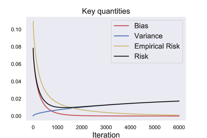
Figure 1: Bias, variance, risk, and empirical risk behavior.

Let us now introduce our ”reference stopping rule”. This stopping rule balances the bias and variance described above, which is a common strategy for model selection in the nonparametric statistics literature, since it usually yields a minimax-optimal estimator (see, e.g., [Tsy08]). This reference stopping rule is defined as the first time the bias term becomes smaller than or equal to the variance term, that is,

$$t^{b}=\inf\{t>0\ |\ B^{2}(t)\leq V(t)\}.$$ (16)

This is a purely theoretical stopping rule since it strongly depends on unknown quantities. However, its main interest lies in the way it compares with the global optimum performance, that is, with the oracle performance. This is the purpose of the next lemma.

Lemma 2.1.

Under the monotonicity of the bias and variance terms,

$$\mathbb{E}_{\varepsilon}\lVert f^{t^{b}}-f^{*}\rVert_{n}^{2}\leq 2\ \underset{t>0}{\inf}\Big{[}\mathbb{E}_{\varepsilon}\lVert f^{t}-f^{*}\rVert_{n}^{2}\Big{]}.$$

Proof of Lemma 2.1.

The proof is quite simple and can be deduced from [BHR16, p.8]. For any $t>0$,

$$B^{2}(t)+V(t)\geq\min\{B^{2}(t^{b}),V(t^{b})\}=\frac{1}{2}\Big{[}B^{2}(t^{b})+V(t^{b})\Big{]}=\frac{1}{2}\mathbb{E}_{\varepsilon}\lVert f^{t^{b}}-f^{*}\rVert_{n}^{2}.$$

To finish the proof, it is sufficient to take $t=\underset{t>0}{\textnormal{argmin}}\Big{[}\mathbb{E}_{\varepsilon}\lVert f^{t}-f^{*}\rVert_{n}^{2}\Big{]}.$ ∎

This lemma provides a fundamental result that guarantees the optimality of $t^{b}$ for any iterative estimator, for which the bias is a non-increasing function of $t$, and the variance is a non-decreasing function of $t$. It also implies that the risk of any spectral filter estimator computed at $t^{b}$ cannot be higher than two times the risk of the oracle rule. This is the main reason for considering $t^{b}$ as a reference stopping rule in our analysis. It is also worth mentioning that even if we knew $B^{2}(t)$ for all $t\leq t_{1}$ for some $t_{1}>0$, the bias could still suddenly drop after at time $t_{2}>t_{1}$. Stopping at $t_{1}$ could then result in a much worse performance than stopping at time $t_{2}$, where the bias term is zero. This remark suggests that recovering the oracle performance cannot be achieved in full generality in the present framework, where one has access to a limited number of ”observations” of the risk curve. This is why the balancing stopping rule $t^{b}$ plays the role of a reference stopping rule since its performance can nevertheless be linked with the one of the oracle stopping rule.

Our main concern is formulating a data-driven stopping rule (a mapping from the data $\{(x_{i},y_{i})\}_{i=1}^{n}$ to a positive time $\widehat{t}$) so that the prediction errors $\mathbb{E}_{\varepsilon}\lVert f^{\widehat{t}}-f^{*}\rVert_{n}^{2}$ or, equivalently, $\mathbb{E}\lVert f^{\widehat{t}}-f^{*}\rVert_{2}^{2}$ are as small as possible. A classical tool commonly used in model selection for quantifying the performance of a procedure is the oracle-type inequality [Cav+02, Kol+06, Tsy08, Wai19]. In the fixed design context, an oracle inequality (in expectation) can be formulated as follows

$$\mathbb{E}_{\varepsilon}\lVert f^{\widehat{t}}-f^{*}\rVert_{n}^{2}\leq C_{n}\underset{t\in\mathcal{T}}{\inf}\Big{[}\mathbb{E}_{\varepsilon}\lVert f^{t}-f^{*}\rVert_{n}^{2}\Big{]}+r_{n},$$ (17)

where the constant $C_{n}\geq 1$ in the right-hand side can depend on various parameters of the problem (except $f^{*}$). The main term $\underset{t\in\mathcal{T}}{\inf}\Big{[}\mathbb{E}_{\varepsilon}\lVert f^{t}-f^{*}\rVert_{n}^{2}\Big{]}$ is the best possible performance any estimator among $\{f^{t},\ t\in\mathcal{T}\}$ can achieve. Ideally, for the oracle inequality to be meaningful, the last term $r_{n}$ in the right-hand side should be negligible compared to the oracle performance.

2.5 Localized empirical Rademacher complexity

The analysis of the forthcoming early stopping rules involves the use of a model complexity measure known as the localized empirical Rademacher complexity [BBM+05, Kol+06, Wai19].

Definition 2.2.

For any given $\epsilon>0$ and a function class $\mathcal{F}$, consider the localized empirical Rademacher complexity

$$\widehat{\mathcal{R}}_{n}(\epsilon,\mathcal{F})=\mathbb{E}_{\mathbf{r}}\left[\underset{\underset{\lVert f\rVert_{n}\leq\epsilon R}{f\in\mathcal{F}}}{\textnormal{sup}}\left|\frac{1}{n}\sum_{i=1}^{n}\mathbf{r}_{i}f(x_{i})\right|\right],$$ (18)

where $\{\mathbf{r}_{i}\}_{i=1}^{n}$ are i.i.d. Rademacher variables ($\{-1,+1\}$-random variables with equal probability $\frac{1}{2}$).

Usually, the localized empirical Rademacher complexity is defined for $R=1$, but due to the scaling factor of $\lVert f^{*}\rVert_{\mathcal{H}}$, one needs to consider the radius $\epsilon R$ within the supremum.

Along the analysis, more explicit lower and upper bounds on the above local empirical Rademacher complexity have to be derived. This is the purpose of introducing the so-called kernel complexity function [Men02, Men03] that is proved to be of the same size (up to numeric constants) as the localized empirical Rademacher complexity of $\mathcal{F}=\mathbb{B}_{\mathcal{H}}(R)$, that is,

$$\widehat{\mathcal{R}}_{n}(\epsilon,\mathcal{H})=R\Big{[}\frac{1}{n}\sum_{j=1}^{r}\textnormal{min}\{\epsilon^{2},\widehat{\mu}_{j}\}\Big{]}^{1/2}.$$ (19)

It corresponds to a rescaled sum of the empirical eigenvalues truncated at $\epsilon^{2}$.

For a given RKHS $\mathcal{H}$ and noise level $\sigma$, let us finally define the empirical critical radius $\widehat{\epsilon}_{n}$ as the smallest positive value $\epsilon$ such that

$$\frac{\widehat{R}_{n}(\epsilon,\mathcal{H})}{\epsilon R}\leq\frac{2\epsilon R}{\sigma}.$$ (20)

There is an extensive literature on the empirical critical equation and related empirical critical radius [Men02, BBM+05, RWY14], and it is out of the scope of the present paper providing an exhaustive review on this topic. Nevertheless, it has been proved that $\widehat{\epsilon}_{n}$ does always exist and is unique. Constant $2$ in Ineq. (20) is for theoretical convenience only.

3 Data-driven early stopping rule and minimum discrepancy principle

Let us start by recalling that the expression of the empirical risk in Eq. (15) gives that the empirical risk is a non-increasing function of $t$ (as illustrated by Fig. 1 as well). This is consistent with the intuition that the amount of available information within the residuals decreases as the number of iterations grows. If there exists an iteration $t$ such that $f^{t}\approx f^{*}$, then the empirical risk is approximately equal to $\sigma^{2}$ (level of noise), that is,

$$\mathbb{E}_{\varepsilon}R_{t}=\mathbb{E}_{\varepsilon}\Big{[}\lVert F^{t}-Y\rVert_{n}^{2}\Big{]}\approx\mathbb{E}_{\varepsilon}\Big{[}\lVert F^{*}-Y\rVert_{n}^{2}\Big{]}=\mathbb{E}_{\varepsilon}\Big{[}\lVert\varepsilon\rVert_{n}^{2}\Big{]}=\sigma^{2}.$$ (21)

Additional iterations would result in fitting to the noise (overfitting). Introducing, moreover, the reduced empirical risk $\widetilde{R}_{t},\ t>0,$ and recalling that $r$ denotes the rank of the Gram matrix, it comes

$$\mathbb{E}_{\varepsilon}R_{t}=\mathbb{E}_{\varepsilon}\Big{[}\frac{1}{n}\sum_{i=1}^{n}(1-\gamma_{i}^{(t)})^{2}Z_{i}^{2}\Big{]}=\mathbb{E}_{\varepsilon}\underbrace{\Big{[}\frac{1}{n}\sum_{i=1}^{r}(1-\gamma_{i}^{(t)})^{2}Z_{i}^{2}\Big{]}}_{\coloneqq\widetilde{R}_{t}}+\frac{n-r}{n}\sigma^{2}\overset{(\textnormal{i})}{\approx}\sigma^{2},$$ (22)

where $(\textnormal{i})$ is due to Eq. (21). This heuristic argument gives rise to a first deterministic stopping rule $t^{*}$ involving the reduced empirical risk and given by

$$t^{*}=\inf\left\{t>0\ |\ \mathbb{E}_{\varepsilon}\widetilde{R}_{t}\leq\frac{r\sigma^{2}}{n}\right\}.$$ (23)

Since $t^{*}$ is not achievable in practice, an estimator of $t^{*}$ is given by the data-driven stopping rule $\tau$ based on the so-called minimum discrepancy principle (MDP)

$$\tau=\inf\left\{t>0\ |\ \widetilde{R}_{t}\leq\frac{r\sigma^{2}}{n}\right\}.$$ (24)

The existing literature considering the MDP-based stopping rule usually defines $\tau$ by the event $\{R_{t}\leq\sigma^{2}\}$ [EHN96, Han10, BM12, BK16, BHR16, Sta19]. On the one hand, with a full-rank kernel ($r=n$), the reduced empirical risk $\widetilde{R}_{t}$ is equal to the classical empirical risk, leading then to the same stopping rule. On the other hand, with a finite-rank kernel ($r\ll n$), using the reduced empirical risk and the event $\{\widetilde{R}_{t}\leq\frac{r\sigma^{2}}{n}\}$ rather than the empirical risk and $\{R_{t}\leq\sigma^{2}\}$ should lead to a less variable stopping rule. From a practical perspective, the knowledge of the rank of the Gram matrix (which is exploited by the reduced empirical risk, unlike the classical empirical risk) avoids estimating the last $n-r$ components of the vector $G^{*}$, which are already known to be zero (see Appendix A for more details).

Intuitively, if the empirical risk is close to its expectation, then $\tau$ should be optimal in some sense. Therefore, the main analysis in the paper will concern quantifying how close $\tau$ and $t^{*}$ are to each other. It appeared in practice that, if the model is quite simple, e.g. the kernel is of finite rank or the variance $\sigma^{2}$ is low compared to the signal $f^{*}$, $\tau$ is close to $t^{*}$, and $\tau$ performs well. As soon as the model becomes complex, e.g. an infinite-rank kernel or the variance $\sigma^{2}$ is high compared to the signal $f^{*}$, $\tau$, as a random variable, has a high variance that should be reduced. Of course, the smoothness of the regression function should play a role too. This not rigorous statement will be further developed in Section 3.2.

3.1 Finite-rank kernels

3.1.1 Fixed-design framework

Let us start by discussing our results with the case of RKHS of finite-rank kernels with rank $r<n:\widehat{\mu}_{i}=0,\ i>r,$ and $\mu_{i}=0,\ i>r$. Examples that include these kernels are the linear kernel $\mathbb{K}(x_{1},x_{2})=x_{1}^{\top}x_{2}$ and the polynomial kernel of degree $d\in\mathbb{N}$ $\mathbb{K}(x_{1},x_{2})=(1+x_{1}^{\top}x_{2})^{d}$. It is easy to show that the polynomial kernel is of finite rank at most $d+1$, meaning that the kernel matrix $K_{n}$ has at most $\min\{d+1,n\}$ nonzero eigenvalues.

The following theorem applies to any functional sequence $\{f^{t}\}_{t=0}^{\infty}$ generated by (11) and initialized at $f^{0}=0$. The main part of the proof of this result consists of properly upper bounding $\mathbb{E}_{\varepsilon}|\mathbb{E}_{\varepsilon}\widetilde{R}_{t^{*}}-\widetilde{R}_{t^{*}}|$ and follows the same trend of Proposition 3.1 in [BHR16].

Theorem 3.1.

Under Assumptions 1 and 2, given the stopping rule (24),

$$\mathbb{E}_{\varepsilon}\lVert f^{\tau}-f^{*}\rVert_{n}^{2}\leq 2(1+\theta^{-1})\mathbb{E}_{\varepsilon}\lVert f^{t^{*}}-f^{*}\rVert_{n}^{2}+2(\sqrt{3}+\theta)\frac{\sqrt{r}\sigma^{2}}{n}$$ (25)

for any positive $\theta$.

Proof of Theorem 3.1.

In this proof, we will use the following inequalities: for any $a,b\geq 0,\ (a-b)^{2}\leq|a^{2}-b^{2}|$, and $2ab\leq\theta a^{2}+\frac{1}{\theta}b^{2}$ for $\forall\theta>0$.

Let us first prove the subsequent oracle-type inequality for the difference between $f^{\tau}$ and $f^{t^{*}}$. Consider

$$\lVert f^{t^{*}}-f^{\tau}\rVert_{n}^{2} =\frac{1}{n}\sum_{i=1}^{r}\Big{(}\gamma_{i}^{(t^{*})}-\gamma_{i}^{(\tau)}\Big{)}^{2}Z_{i}^{2}\leq\frac{1}{n}\sum_{i=1}^{r}|(1-\gamma_{i}^{(t^{*})})^{2}-(1-\gamma_{i}^{(\tau)})^{2}|Z_{i}^{2}$$

$$=(\widetilde{R}_{t^{*}}-\widetilde{R}_{\tau})\mathbb{I}\left\{\tau\geq t^{*}\right\}+(\widetilde{R}_{\tau}-\widetilde{R}_{t^{*}})\mathbb{I}\left\{\tau<t^{*}\right\}$$

$$\leq(\widetilde{R}_{t^{*}}-\mathbb{E}_{\varepsilon}\widetilde{R}_{t^{*}})\mathbb{I}\left\{\tau\geq t^{*}\right\}+(\mathbb{E}_{\varepsilon}\widetilde{R}_{t^{*}}-\widetilde{R}_{t^{*}})\mathbb{I}\left\{\tau<t^{*}\right\}$$

$$\leq|\widetilde{R}_{t^{*}}-\mathbb{E}_{\varepsilon}\widetilde{R}_{t^{*}}|.$$

From the definition of $\widetilde{R}_{t}$ (22), one notices that

$$|\widetilde{R}_{t^{*}}-\mathbb{E}_{\varepsilon}\widetilde{R}_{t^{*}}| =\left|\sum_{i=1}^{r}(1-\gamma_{i}^{(t^{*})})^{2}\Big{[}\frac{1}{n}(\varepsilon_{i}^{2}-\sigma^{2})+\frac{2}{n}\varepsilon_{i}G_{i}^{*}\Big{]}\right|.$$

From $\mathbb{E}_{\varepsilon}|X(\varepsilon)|\leq\sqrt{\text{var}_{\varepsilon}X(\varepsilon)}$ for $X(\varepsilon)$ centered and $\sqrt{a+b}\leq\sqrt{a}+\sqrt{b}$ for any $a,b\geq 0$, and $\mathbb{E}_{\varepsilon}\left(\varepsilon^{4}\right)\leq 3\sigma^{4}$, it comes

$$\mathbb{E}_{\varepsilon}|\widetilde{R}_{t^{*}}-\mathbb{E}_{\varepsilon}\widetilde{R}_{t^{*}}| \leq\sqrt{\frac{2\sigma^{2}}{n^{2}}\sum_{i=1}^{r}(1-\gamma_{i}^{(t^{*})})^{4}\left[\frac{3}{2}\sigma^{2}+2(G_{i}^{*})^{2}\right]}$$

$$\leq\sqrt{\frac{3\sigma^{4}}{n^{2}}\sum_{i=1}^{r}(1-\gamma_{i}^{(t^{*})})^{2}}+\sqrt{\frac{4\sigma^{2}}{n^{2}}\sum_{i=1}^{r}(1-\gamma_{i}^{(t^{*})})^{2}(G_{i}^{*})^{2}}$$

$$\leq\frac{\sqrt{3}\sigma^{2}\sqrt{r}}{n}+\theta\frac{\sigma^{2}}{n}+\theta^{-1}B^{2}(t^{*})$$

$$\leq\theta^{-1}B^{2}(t^{*})+(\sqrt{3}+\theta)\frac{\sqrt{r}\sigma^{2}}{n}.$$

Applying the inequalities $(a+b)^{2}\leq 2a^{2}+2b^{2}$ for any $a,b\geq 0$ and $B^{2}(t^{*})\leq\mathbb{E}_{\varepsilon}\lVert f^{t^{*}}-f^{*}\rVert_{n}^{2}$, we arrive at

$$\mathbb{E}_{\varepsilon}\lVert f^{\tau}-f^{*}\rVert_{n}^{2}$$

$$\leq 2\mathbb{E}_{\varepsilon}\lVert f^{t^{*}}-f^{*}\rVert_{n}^{2}+2\mathbb{E}_{\varepsilon}\lVert f^{\tau}-f^{t^{*}}\rVert_{n}^{2}$$

$$\leq 2(1+\theta^{-1})\mathbb{E}_{\varepsilon}\lVert f^{t^{*}}-f^{*}\rVert_{n}^{2}+2(\sqrt{3}+\theta)\frac{\sqrt{r}\sigma^{2}}{n}.$$

The claim is proved. ∎

First of all, it is worth noting that the risk of the estimator $f^{t^{*}}$ is proved to be optimal for gradient descent and kernel ridge regression no matter the kernel we use (see Appendix C for the proof), so it remains to focus on the remainder term on the right-hand side in Ineq. (25). Theorem 3.1 applies to any reproducing kernel, but one remarks that for infinite-rank kernels, $r=n$, and we achieve only the rate $\mathcal{O}(1/\sqrt{n})$. This rate is suboptimal since, for instance, RKHS with polynomial eigenvalue decay kernels (will be considered in the next subsection) has the minimax-optimal rate for the risk error of the order $\mathcal{O}(n^{-\frac{\beta}{\beta+1}})$, with $\beta>1$. Therefore, the oracle-type inequality (25) could be useful only for finite-rank kernels due to the fast $\mathcal{O}(\sqrt{r}/n)$ rate of the remainder term.

Notice that, in order to make artificially the term $\mathcal{O}(\frac{\sqrt{r}}{n})$ a remainder one (even for cases corresponding to infinite-rank kernels), [BHR16, BHR+18] introduced in the definitions of their stopping rules a restriction on the ”starting time” $t_{0}$. However, in the mentioned work, this restriction incurred the price of possibility to miss the designed time $\tau$. For instance, in [BHR16], the authors took $t_{0}$ as the first time at which the variance becomes of the order $\frac{\sqrt{r}\sigma^{2}}{n}(\sqrt{D}\delta^{2}$ in their notations). Besides that, [BHR+18] developed an additional procedure based on standard model selection criteria such as AIC-criterion for the spectral cut-off estimator to recover the ”missing” stopping rule and to achieve optimality over Sobolev-type ellipsoids. In our work, we removed such a strong assumption.

As a corollary of Theorem 3.1, one can prove that $f^{\tau}$ provides a minimax estimator of $f^{*}$ over the ball of radius $R$.

Corollary 3.2.

Under Assumptions 1, 2, 3, if a kernel has finite rank $r$, then

$$\mathbb{E}_{\varepsilon}\lVert f^{\tau}-f^{*}\rVert_{n}^{2}\leq c_{u}R^{2}\widehat{\epsilon}_{n}^{2},$$ (26)

where the constant $c_{u}$ is numeric.

Proof of Corollary 3.2.

From Theorem 3.1 and Lemma C.1 in Appendix,

$$\mathbb{E}_{\varepsilon}\lVert f^{\tau}-f^{*}\rVert_{n}^{2}\leq 16(1+\theta^{-1})R^{2}\widehat{\epsilon}_{n}^{2}+2(\sqrt{3}+\theta)\frac{\sqrt{r}\sigma^{2}}{n}.$$ (27)

Further, from Lemma A.4 in Appendix, $\widehat{\epsilon}_{n}^{2}=c\frac{r\sigma^{2}}{nR^{2}}$ with a positive numeric constant $c$, and it implies that

$$\mathbb{E}_{\varepsilon}\lVert f^{\tau}-f^{*}\rVert_{n}^{2}\leq\Big{[}16(1+\theta^{-1})+\frac{2(\sqrt{3}+\theta)}{c}\Big{]}R^{2}\widehat{\epsilon}_{n}^{2}.$$ (28)

∎

Note that the critical radius $\widehat{\epsilon}_{n}$ cannot be arbitrary small since it should satisfy Ineq. (20). As it will be clarified later, the squared empirical critical radius is essentially optimal.

3.1.2 Random-design framework

We would like to transfer the minimax optimality bound for the estimator $f^{\tau}$ from the empirical $L_{2}(\mathbb{P}_{n})$-norm to the $L_{2}(\mathbb{P}_{X})$ in-sample norm by means of the so-called localized population Rademacher complexity. This complexity measure became a standard tool in empirical processes and nonparametric regression [BBM+05, Kol+06, RWY14, Wai19].

For any kernel function class studied in the paper, we consider the localized Rademacher complexity that can be seen as a population counterpart of the empirical Rademacher complexity (19) introduced earlier:

$$\overline{\mathcal{R}}_{n}(\epsilon,\mathcal{H})=R\left[\frac{1}{n}\sum_{i=1}^{\infty}\min\{\mu_{i},\epsilon^{2}\}\right]^{1/2}.$$ (29)

Using the localized population Rademacher complexity, we define its population critical radius $\epsilon_{n}>0$ to be the smallest positive solution $\epsilon$ that satisfies the inequality

$$\frac{\overline{\mathcal{R}}_{n}(\epsilon,\mathcal{H})}{\epsilon R}\leq\frac{2\epsilon R}{\sigma}.$$ (30)

In contrast to the empirical critical radius $\widehat{\epsilon}_{n}$, this quantity is not data-dependent, since it is specified by the population eigenvalues of the kernel operator $T_{k}$ underlying the RKHS.

Recall the definition of the population critical radius (30), then the following result provides a fundamental lemma of the transfer between the $L_{2}(\mathbb{P}_{n})$ and $L_{2}(\mathbb{P}_{X})$ functional norms. In what follows, we assume that $\mathcal{H}$ is a star-shaped function class, meaning that for any $f\in\mathcal{H}$ and scalar $\omega\in[0,1],$ the function $\omega f$ belongs to $\mathcal{H}$. The assumption on $\mathcal{H}$ being star-shape holds if $f$ is assumed to lie in the $\mathcal{H}$-norm ball of an arbitrary finite radius.

Lemma 3.3.

[Wai19, Theorem 14.1] Assume a star-shaped kernel function class $\mathcal{H}$ and Assumption 2 of bounded kernel. Let $\epsilon_{n}$ be as in Ineq. (30), then for any $f\in\mathbb{B}_{\mathcal{H}}(cR)$, where $c>1$ is a numeric constant, and any $h\geq\epsilon_{n}$, one has

$$\left|\lVert f\rVert_{n}^{2}-\lVert f\rVert_{2}^{2}\right|\leq\frac{1}{2}\lVert f\rVert_{2}^{2}+c_{1}R^{2}h^{2}$$ (31)

with probability at least $1-c_{2}e^{-c_{3}\frac{nh^{2}R^{2}}{\sigma^{2}}}$, for some positive numeric constants $c_{1},c_{2}$, and $c_{3}$.

We deduce from Lemma 3.3 that with probability at least $1-c_{2}e^{-c_{3}\frac{nh^{2}R^{2}}{\sigma^{2}}}$,

$$\frac{1}{2}\lVert f\rVert_{2}^{2}-c_{1}R^{2}h^{2}\leq\lVert f\rVert_{n}^{2}\leq\frac{3}{2}\lVert f\rVert_{2}^{2}+c_{1}R^{2}h^{2}.$$

The previous lemma means the following. If we are able to proof that for some $t>0$, $\lVert f^{t}-f^{*}\rVert_{\mathcal{H}}^{2}\leq cR$ with high probability for a positive numeric constant $c$, then we can directly change the optimality result in terms of $\lVert f^{t}-f^{*}\rVert_{n}^{2}$ to the optimality result in terms of the $L_{2}(\mathbb{P}_{X})$-norm $\lVert f^{t}-f^{*}\rVert_{2}^{2}$, losing only $c_{1}R^{2}h^{2}\asymp R^{2}\epsilon_{n}^{2}$ by choosing $h=\epsilon_{n}$.

Equipped with the localized Rademacher complexity (29), we can state the optimality theorem for finite-rank kernels for any functional sequence $\{f^{t}\}_{t=0}^{\infty}$ generated by (11) and initialized at $f^{0}=0$.

Theorem 3.4.

Under Assumptions 1, 2, and 3, given the stopping rule (24), there is a numeric constant $\widetilde{c}_{u}$ so that for finite-rank kernels with rank $r$,

$$\mathbb{E}\lVert f^{\tau}-f^{*}\rVert_{2}^{2}\leq\widetilde{c}_{u}\frac{r\sigma^{2}}{n}.$$ (32)

Proof intuition. The full proof is deferred to Section F. Its main ingredient is Lemma H.2 in Appendix that states the following: $\lVert f^{t}\rVert_{\mathcal{H}}\leq\sqrt{7}R$ for any $t\leq\overline{t}_{\epsilon}$, where $\overline{t}_{\epsilon}=\inf\Big{\{}t>0\ |\ B^{2}(t)=\frac{\sigma^{2}}{2n}\sum_{i=1}^{r}\gamma_{i}^{(t)}\Big{\}}$, with high probability. With this argument, we can apply the triangular inequality and Lemma 3.3, if $\tau\leq\overline{t}_{\epsilon}$ w.h.p.

Remark.

Theorem 3.4 provides a rate for the $L_{2}(\mathbb{P}_{X})$-norm that matches up to a constant the minimax bound (see, e.g., [RWY12, Theorem 2(a)] with $s=d=1$), when $f^{*}$ belongs to the $\mathcal{H}$-norm ball of a fixed radius $R$, thus not improvable in general. A similar bound for finite-rank kernels was achieved in [RWY14, Corollary 4].

We summarize our findings in the following corollary.

Corollary 3.5.

Under Assumptions 1, 2, 3, and a finite-rank kernel, the early stopping rule $\tau$ satisfies

$$\mathbb{E}\lVert f^{\tau}-f^{*}\rVert_{2}^{2}\asymp\underset{\widehat{f}}{\inf}\underset{\lVert f^{*}\rVert_{\mathcal{H}}\leq R}{\sup}\mathbb{E}\lVert\widehat{f}-f^{*}\rVert_{2}^{2},$$ (33)

where the infimum is taken over all measurable functions of the input data.

3.2 Practical behavior of $\tau$ with infinite-rank kernels

A typical example of RKHS that produces a ”smooth” infinite-rank kernel is the $k^{\textnormal{th}}$-order Sobolev spaces for some fixed integer $k\geq 1$ with Lebesgue measure on a bounded domain. We consider Sobolev spaces that consist of functions that have $k^{\textnormal{th}}$-order weak derivatives $f^{(k)}$ being Lebesgue integrable and $f^{(0)}=f^{(1)}(0)=\ldots=f^{(k-1)}(0)=0$. It is worth to mention that for such classes, the eigenvalues of the Gram matrix $\widehat{\mu}_{i}\asymp i^{-\beta},\ i\in[r]$. Another example of kernel with this decay condition for the eigenvalues is the Laplace kernel $\mathbb{K}(x_{1},x_{2})=e^{-|x_{1}-x_{2}|},\ x_{1},x_{2}\in\mathbb{R}$ (see, [SS01] p.402).

Firstly, let us now illustrate the practical behavior of ESR (24) (its histogram) for gradient descent (11) with the step-size $\eta=1/(1.2\widehat{\mu}_{1})$ and one-dimensional Sobolev kernel $\mathbb{K}(x_{1},x_{2})=\min\{x_{1},x_{2}\}$ that generates the reproducing space

$$\mathcal{H}=\left\{f:[0,1]\to\mathbb{R}\ |\ f(0)=0,\int_{0}^{1}(f^{\prime}(x))^{2}dx<\infty\right\}.$$ (34)

We deal with the model (1) with two regression functions: a smooth piece-wise linear $f^{*}(x)=|x-1/2|-1/2$ and nonsmooth heavisine $f^{*}(x)=0.093\ [4\ \textnormal{sin}(4\pi x)-\textnormal{sign}(x-0.3)-\textnormal{sign}(0.72-x)]$ functions. The design points are random $x_{i}\overset{\textnormal{i.i.d.}}{\sim}\mathbb{U}[0,1]$. The number of observations is $n=200$. For both functions, $\lVert f^{*}\rVert_{n}\approx 0.28$, and we set up a middle difficulty noise level $\sigma=0.15$. The number of repetitions is $N=200$.

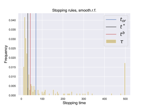
(a)

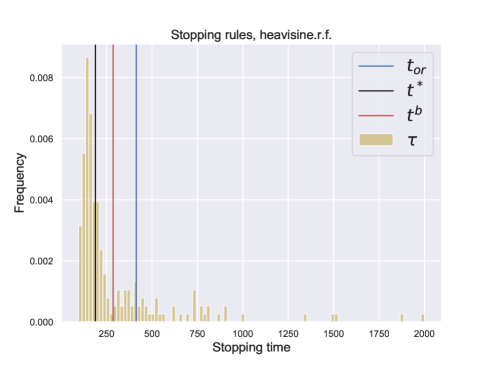
(b)

Figure 2: Histogram of $\tau$ vs $t^{b}$ vs $t^{*}$ vs $t_{\textnormal{or}}\coloneqq\underset{t>0}{\textnormal{argmin}}\Big{[}\mathbb{E}_{\varepsilon}\lVert f^{t}-f^{*}\rVert_{n}^{2}\Big{]}$ for kernel gradient descent with the step-size $\eta=1/(1.2\widehat{\mu}_{1})$ for the piece-wise linear $f^{*}(x)=|x-1/2|-1/2$ (panel (a)) and heavisine $f^{*}(x)=0.093\ [4\ \textnormal{sin}(4\pi x)-\textnormal{sign}(x-0.3)-\textnormal{sign}(0.72-x)]$ (panel (b)) regression functions, and the first-order Sobolev kernel $\mathbb{K}(x_{1},x_{2})=\min\{x_{1},x_{2}\}$.

In panel (a) of Figure 2, we detect that our stopping rule $\tau$ has a high variance. This could be explained by the variability of $\tau$ around its proxy version $t^{*}$ or by the variability of the empirical risk $R_{t}$ around its expectation at $t^{*}$. To understand this phenomenon, we move back to Theorem 3.1 and notice that the remainder term there vanishes at the fast rate $\mathcal{O}(\sqrt{r}/n)$ when the kernel rank is fixed. If the kernel is not of finite rank, as a consequence, the worst-case rate is $\mathcal{O}(1/\sqrt{n})$, and we could not guarantee that we get a true remainder term at the end. Thus, the high variance comes from a large remainder term. Moreover, it has been shown in [BHR+18] that the term $\mathcal{O}(\sqrt{r}/n)$ is unavoidable for the spectral cut-off algorithm (in their notation, it corresponds to $\sqrt{D}\delta^{2}$ where $\delta^{2}=\frac{\sigma^{2}}{n}$).

If we change the signal $f^{*}$ from the smooth to nonsmooth one, the regression function does not belong anymore to $\mathcal{H}$ defined in (34). In this case (panel (b) in Figure 2), the stopping rule $\tau$ performs much better than for the previous regression function. A conclusion one can make is that for smooth functions in $\mathcal{H}$, one needs to reduce the variance of the empirical risk. In order to do that and to get a stable early stopping rule that will be close to $t^{*}$, we propose using a special smoothing technique for the empirical risk.

4 Polynomial smoothing

As was mentioned earlier, the main issue of poor behavior of the stopping rule $\tau$ for ”smooth” infinite-rank kernels is the variability of the empirical risk around its expectation. We would like to reduce this variability. In order to grasp additional intuition of this variability, consider the expectation of the empirical risk $\mathbb{E}_{\varepsilon}R_{t}\approx\frac{1}{n}\sum_{i=1}^{r}(1-\gamma_{i}^{(t)})^{2}(G^{*}_{i})^{2}$ and the fact that there exist components $i\in[r]$ for which $(G^{*}_{i})^{2}\leq\varepsilon_{i}^{2}$, one can conclude that there is no hope to apply the early stopping $\tau$ with this type of kernels. That would be extremely difficult to recover the part of the regression function associated with these components since we observe pure noise. Our goal then is to reduce the number of these components and, by doing that, to reduce the variability of the empirical risk. A solution that we propose is to smooth the empirical risk by means of the eigenvalues of the normalized Gram matrix.

4.1 Polynomial smoothing and minimum discrepancy principle rule

We start by defining the squared $\alpha$-norm as $\lVert f\rVert_{n,\alpha}^{2}\coloneqq\langle K_{n}^{\alpha}F,F\rangle_{n}$ for all $F=\left[f(x_{1}),\ldots,f(x_{n})\right]^{\top}\in\mathbb{R}^{n}$ and $\alpha\in[0,1]$, from which we also introduce the smoothed risk, bias, and variance of a spectral filter estimator as

$$R_{\alpha}(t)=\mathbb{E}_{\varepsilon}\lVert f^{t}-f^{*}\rVert_{n,\alpha}^{2}=\lVert\mathbb{E}_{\varepsilon}f^{t}-f^{*}\rVert_{n,\alpha}^{2}+\mathbb{E}_{\varepsilon}\lVert f^{t}-\mathbb{E}_{\varepsilon}f^{t}\rVert_{n,\alpha}^{2}=B^{2}_{\alpha}(t)+V_{\alpha}(t),$$

with

$$B^{2}_{\alpha}(t)=\frac{1}{n}\sum_{i=1}^{r}\widehat{\mu}_{i}^{\alpha}(1-\gamma_{i}^{(t)})^{2}(G_{i}^{*})^{2},\ \ \ \ V_{\alpha}(t)=\frac{\sigma^{2}}{n}\sum_{i=1}^{r}\widehat{\mu}_{i}^{\alpha}(\gamma_{i}^{(t)})^{2}.$$ (35)

The smoothed empirical risk is

$$R_{\alpha,t}=\lVert F^{t}-Y\rVert_{n,\alpha}^{2}=\lVert G^{t}-Z\rVert_{n,\alpha}^{2}=\frac{1}{n}\sum_{i=1}^{r}\widehat{\mu}_{i}^{\alpha}(1-\gamma_{i}^{(t)})^{2}Z_{i}^{2},\quad\textnormal{ for }t>0.$$ (36)

Recall that the kernel is bounded by $B=1$, thus $\widehat{\mu}_{i}\leq 1$ for all $i=1,\ldots,r$, then the smoothed bias $B_{\alpha}^{2}(t)$ and smoothed variance $V_{\alpha}(t)$ are smaller their non-smoothed counterparts.

Analogously to the heuristic derivation leading to the stopping rule (24), the new stopping rule is based on the discrepancy principle applied to the $\alpha-$smoothed empirical risk, that is,

$$\tau_{\alpha}=\inf\left\{t>0\ |\ R_{\alpha,t}\leq\sigma^{2}\frac{\mathrm{tr}(K_{n}^{\alpha})}{n}\right\},$$ (37)

where $\sigma^{2}\mathrm{tr}(K_{n}^{\alpha})/n=\sigma^{2}\sum_{i=1}^{r}\widehat{\mu}_{i}^{\alpha}/n$ is the natural counterpart of $r\sigma^{2}/n$ in the case of a full-rank kernel and the $\alpha-$norm.

Since there is no straightforward connection between $\tau_{\alpha}$ and the former reference stopping rule $t^{b}=\inf\{t>0\ |\ B^{2}(t)\leq V(t)\}$, we need to introduce a new reference one for the theoretical analysis of the behavior of $\tau_{\alpha}$. We first define a new smoothed reference stopping rule (which balances between the smoothed bias and variance)

$$t^{b}_{\alpha}=\inf\left\{t>0\ |\ B^{2}_{\alpha}(t)\leq V_{\alpha}(t)\right\}$$ (38)

and also the analogue of (23) with the $\alpha-$norm:

$$t_{\alpha}^{*}=\inf\left\{t>0\ |\ \mathbb{E}_{\varepsilon}R_{\alpha,t}\leq\frac{\sigma^{2}}{n}\sum_{i=1}^{r}\widehat{\mu}_{i}^{\alpha}\right\}.$$ (39)

4.2 Related work

The idea of smoothing the empirical risk (the residuals) is not new in the literature. For instance, [BM10, BM12, BK16] discussed various smoothing strategies applied to (kernelized) conjugate gradient descent, and [CW20] considered spectral regularization with spectral filter estimators. More closely related to the present work, [Sta19] studied a statistical performance improvement allowed by polynomial smoothing of the residuals (as we do here) but restricted to the spectral cut-off estimator.

In [BM10, BM12], the authors considered the following statistical inverse problem: $z=Ax+\sigma\zeta$, where $A$ is a self-adjoint operator and $\zeta$ is Gaussian noise. In their case, for the purpose of achieving optimal rates, the usual discrepancy principle rule $\lVert Ax_{m}-z\rVert\leq\vartheta\delta$ ($m$ is an iteration number, $\vartheta$ is a parameter) was modified and took the form $\lVert\rho_{\lambda}(A)(Ax_{m}-z)\rVert\leq\vartheta\delta$, where $\rho_{\lambda}(t)=\frac{1}{\sqrt{t+\lambda}}$ and $\delta$ is the normalized variance of Gaussian noise.

In [BK16], the minimum discrepancy principle was modified to the following: each iteration $m$ of conjugate gradient descent was represented by a vector $\widehat{\alpha}_{m}=K_{n}^{\dagger}Y$, $K_{n}^{\dagger}$ is the pseudo-inverse of the normalized Gram matrix, and the learning process was stopped if $\lVert Y-K_{n}\widehat{\alpha}_{m}\rVert_{K_{n}}<\Omega$ for some positive $\Omega$, where $\lVert\alpha\rVert_{K_{n}}^{2}=\langle\alpha,K_{n}\alpha\rangle.$ Thus, this method corresponds (up to a threshold) to the stopping rule (37) with $\alpha=1.$

In the work [Sta19], the authors concentrated on the inverse problem $Y=A\xi+\delta W$ and its corresponding Gaussian vector observation model $Y_{i}=\tilde{\mu}_{i}\xi_{i}+\delta\varepsilon_{i},\ i\in[r]$, where $\{\tilde{\mu}_{i}\}_{i=1}^{r}$ are the singular values of the linear bounded operator $A$ and $\{\varepsilon_{i}\}_{i=1}^{r}$ are Gaussian noise variables. They recovered the signal $\{\xi_{i}\}_{i=1}^{r}$ by a cut-off estimator of the form $\widehat{\xi}_{i}^{(t)}=\mathbb{I}\{i\leq t\}\widetilde{\mu}_{i}^{-1}Y_{i},\ i\in[r]$. The discrepancy principle in this case was $\lVert(AA^{\top})^{\alpha/2}(Y-A\widehat{\xi}^{(t)})\rVert^{2}\leq\kappa$ for some positive $\kappa.$ They found out that, if the smoothing parameter $\alpha$ lies in the interval $[\frac{1}{4p},\frac{1}{2p})$, where $p$ is the polynomial decay of the singular values $\{\widetilde{\mu}_{i}\}_{i=1}^{r}$, then the cut-off estimator is adaptive to Sobolev ellipsoids. Therefore, our work could be considered as an extension of [Sta19] in order to generalize the polynomial smoothing strategy to more complex filter estimators such as gradient descent and (Tikhonov) ridge regression in the reproducing kernel framework.

4.3 Optimality result (fixed-design)

To take into account in our analysis the fact that we use the $\alpha-$norm, we define a modified version of the localized empirical Rademacher complexity that we call the smoothed empirical Rademacher complexity. The derivation of the next expression is deferred to Appendix G.

Definition 4.1.

The smoothed empirical Rademacher complexity of $\mathbb{B}_{\mathcal{H}}(R)$ is defined as

$$\widehat{\mathcal{R}}_{n,\alpha}(\epsilon,\mathcal{H})=R\sqrt{\frac{1}{n}\sum_{i=1}^{r}\widehat{\mu}_{i}^{\alpha}\min\{\widehat{\mu}_{i},\epsilon^{2}\}},$$ (40)

where $\alpha\in[0,1]$ and $\{\widehat{\mu}_{i}\}_{i=1}^{r}$ are the eigenvalues of the Gram matrix $K_{n}$.

This new definition leads to the next updated smoothed version of the critical inequality and its related empirical critical radius.

Definition 4.2.

Define the smoothed empirical critical radius $\widehat{\epsilon}_{n,\alpha}$ as the smallest positive solution $\epsilon>0$ to the following fixed-point inequality

$$\frac{\widehat{\mathcal{R}}_{n,\alpha}(\epsilon,\mathcal{H})}{\epsilon R}\leq\frac{2R}{\sigma}\epsilon^{1+\alpha}.$$ (41)

Appendix H establishes that the smoothed empirical critical radius $\widehat{\epsilon}_{n,\alpha}$ does exist, is unique and achieves the equality in Ineq. (41).

We pursue the analogy a bit further by defining the smoothed statistical dimension as

$$d_{n,\alpha}\coloneqq\min\Big{\{}j\in[r]:\widehat{\mu}_{j}\leq\widehat{\epsilon}_{n,\alpha}^{2}\Big{\}},$$ (42)

and $d_{n,\alpha}=r$ if no such index does exist. Combined with (40), this implies that

$$\widehat{\mathcal{R}}_{n,\alpha}^{2}(\widehat{\epsilon}_{n,\alpha},\mathcal{H})\geq\frac{\sum_{j=1}^{d_{n,\alpha}}\widehat{\mu}_{j}^{\alpha}}{n}R^{2}\widehat{\epsilon}_{n,\alpha}^{2},\quad\textnormal{ and }\quad\widehat{\epsilon}_{n,\alpha}^{2(1+\alpha)}\geq\frac{\sigma^{2}\sum_{j=1}^{d_{n,\alpha}}\widehat{\mu}_{j}^{\alpha}}{4R^{2}n},$$ (43)

where the second statement results from Ineq. (41). Let us emphasize that [YPW17] already introduced the so-called statistical dimension (corresponds to $\alpha=0$ in our notations). It appeared that the statistical dimension provides an upper bound on the minimax-optimal dimension of randomized projections for kernel ridge regression (see [YPW17, Theorem 2, Corollary 1]).

In our case, $d_{n,\alpha}$ can be seen as a ($\alpha$-smooth) version of the statistical dimension. One motivation is that this notion turns out to be useful in the derivation of minimax rates. In particular, this can be achieved by means of the following assumptions that involve this quantity.

Assumption 4.

There exists a numeric $\mathcal{A}>0$ such that for all $\alpha\in[0,1]$,

$$\sum_{i=d_{n,\alpha}+1}^{r}\widehat{\mu}_{i}\leq\mathcal{A}d_{n,\alpha}\widehat{\epsilon}_{n,\alpha}^{2}.$$ (44)

This assumption will further make the transfer from the smooth critical inequality (41) to its non-smooth version (20). Indeed, under Assumption 4, if $\epsilon$ satisfies Ineq. (41), then it satisfies Ineq. (20) as well, where constant $2$ on the right-hand side is replaced by $2\sqrt{1+\mathcal{A}}$. Although there are reproducing kernels for which Assumption 4 does not hold, for most of them it holds true [YPW17], including all the examples in the present paper. We detail one of them below.

Example 1 ($\beta$-polynomial eigenvalue decay).

Let us assume that the eigenvalues of the normalized Gram matrix satisfy that there exist numeric constants $0<c\leq C$ such that

$$ci^{-\beta}\leq\widehat{\mu}_{i}\leq Ci^{-\beta},\quad i=1,\ldots,r,$$ (45)

for some $\beta>1$. Instances of kernels in this class are mentioned at the beginning of Section 3.2. Then, Assumption 4 holds with $\mathcal{A}=\frac{C}{c}\frac{1}{\beta-1}$.

Another key property for the smoothing to yield optimal results is that the value of $\alpha$ has to be large enough to control the tail sum of the smoothed eigenvalues by the corresponding cumulative sum, which is the purpose of the assumption below.

Assumption 5.

There exists $\Upsilon=[\alpha_{0},1],\ \alpha_{0}\geq 0$, such that for all $\alpha\in\Upsilon$,

$$\sum_{i=d_{n,\alpha}+1}^{r}\widehat{\mu}_{i}^{2\alpha}\leq\mathcal{M}\sum_{i=1}^{d_{n,\alpha}}\widehat{\mu}_{i}^{2\alpha},$$ (46)

where $\mathcal{M}\geq 1$ denotes a numeric constant.

Let us remark that controlling the tail sum of the empirical eigenvalues has been already made, for example, by [Bar+20] (effective rank) and more recently by [CW20, Assumption 6]. Let us also mention that Assumption 5 does not imply Assumption 4 holds.

Let us enumerate several classical examples for which this assumption holds.

Example 2 ($\beta$-polynomial eigenvalue decay kernels (45)).

For the polynomial eigenvalue-decay kernels, Assumption 5 holds with

$$\mathcal{M}=2\Big{(}\frac{C}{c}\Big{)}^{2}\quad\textnormal{and}\quad 1\geq\alpha\geq\frac{1}{\beta+1}=\alpha_{0}.$$ (47)

Example 3 ($\gamma$-exponential eigenvalue-decay kernels).

Let us assume that the eigenvalues of the normalized Gram matrix satisfy that there exist numeric constants $0<c\leq C$ and a constant $\gamma>0$ such that

$$ce^{-i^{\gamma}}\leq\widehat{\mu}_{i}\leq Ce^{-i^{\gamma}}.$$

Instances of kernels within this class include the Gaussian kernel with respect to the Lebesgue measure on the real line (with $\gamma=2$) or on a compact domain (with $\gamma=1$) (up to $\log$ factor in the exponent). Then, Assumption 5 holds with

$$\mathcal{M}=\Big{(}\frac{C}{c}\Big{)}^{2}\frac{\int_{0}^{\infty}e^{-y^{\gamma}}dy}{\int_{(2\alpha_{0})^{1/\gamma}}^{2(2\alpha_{0})^{1/\gamma}}e^{-y^{\gamma}}dy}\quad\textnormal{and}\quad\alpha\in[\alpha_{0},1],\quad\mbox{for any}\quad\alpha_{0}\in(0,1).$$

For any reproducing kernel satisfying the above assumptions, the next theorem provides a high probability bound on the performance of $f^{\tau_{\alpha}}$ (measured in terms of the $L_{2}(\mathbb{P}_{n})$-norm), which depends on the smoothed empirical critical radius.

Theorem 4.1 (Upper bound).

Under Assumptions 1, 2, 3, 4, and 5, given the stopping rule (37),

$$\lVert f^{\tau_{\alpha}}-f^{*}\rVert_{n}^{2}\leq c_{u}R^{2}\widehat{\epsilon}_{n,\alpha}^{2}$$ (48)

with probability at least $1-5\exp\Big{[}-c_{1}\frac{R^{2}}{\sigma^{2}}n\widehat{\epsilon}_{n,\alpha}^{2(1+\alpha)}\Big{]}$ for some positive constants $c_{1}$ and $c_{u}$, where $c_{1}$ depends only on $\mathcal{M}$, $c_{u}$ depends only on $\mathcal{A}$.

Moreover,

$$\mathbb{E}_{\varepsilon}\lVert f^{\tau_{\alpha}}-f^{*}\rVert_{n}^{2}\leq CR^{2}\widehat{\epsilon}_{n,\alpha}^{2}+6\max\{\sigma^{2},R^{2}\}\exp\Big{[}-c_{3}\frac{R^{2}}{\sigma^{2}}n\widehat{\epsilon}_{n,\alpha}^{2(1+\alpha)}\Big{]},$$ (49)

for the constant $C$ only depending on $\mathcal{A}$, constant $c_{3}$ only depending on $\mathcal{M}$.

First of all, Theorem 4.1 is established in the fixed-design framework, and Ineq. (49) is a direct consequence of the high probability bound (48). The main message is that the final performance of the estimator $f^{\tau_{\alpha}}$ is controlled by the smoothed critical radius $\widehat{\epsilon}_{n,\alpha}$. From the existing literature on the empirical critical radius [RWY12, RWY14, YPW17, Wai19], it is already known that the non-smooth version $\widehat{\epsilon}_{n}^{2}$ is the typical quantity that leads to minimax rates in the RKHS (see also Theorem 4.2 below). In particular, tight upper bounds on $\widehat{\epsilon}_{n}^{2}$ can be computed from a priori information about the RKHS, e.g. the decay rate of the empirical/population eigenvalues. However, the behavior of $\widehat{\epsilon}_{n,\alpha}^{2}$ with respect to $n$ is likely to depend on $\alpha$, as emphasized by the notation. Intuitively, this suggests that there could exist a range of values of $\alpha$, for which $\widehat{\epsilon}_{n,\alpha}^{2}$ is of the same order as (or faster than) $\widehat{\epsilon}_{n}^{2}$, leading therefore to optimal rates. But there could also exist ranges of values of $\alpha$, where this does not hold true, leading to suboptimal rates.

Another striking aspect of Ineq. (49) is related to the additional terms involving the exponential function in Ineq. (49). As far as (48) is a statement with ”high probability”, this term is expected to converge to 0 at a rate depending on $n\widehat{\epsilon}_{n,\alpha}^{2}$. Therefore, the final convergence rate as well as the fact that this term is (or not) negligible will depend on $\alpha$.

Sketch of the proof of Theorem 4.1.

The complete proof is given in Appendix D and starts from splitting the risk error $\lVert f^{\tau_{\alpha}}-f^{*}\rVert_{n}^{2}$ into two parts:

$$2B^{2}(\tau_{\alpha})+2v(\tau_{\alpha}),$$ (50)

where $v(t)\coloneqq\frac{1}{n}\sum_{i=1}^{n}(\gamma_{i}^{(t)})^{2}\varepsilon_{i}^{2}$ is called the stochastic variance at iteration $t$.

The key ingredients of the proof are the next two deviation inequalities.

$$i)\ \mathbb{P}_{\varepsilon}\left(\tau_{\alpha}>\overline{t}_{\epsilon,\alpha}\right) \leq 2\ \exp\Big{[}-c_{1}\frac{R^{2}}{\sigma^{2}}n\widehat{\epsilon}_{n,\alpha}^{2(1+\alpha)}\Big{]},$$

$$ii)\ \mathbb{P}_{\varepsilon}\left(\tau_{\alpha}<\widetilde{t}_{\epsilon,\alpha}\right) \leq 2\ \exp\Big{[}-c_{2}\frac{R^{2}}{\sigma^{2}}n\widehat{\epsilon}_{n,\alpha}^{2(1+\alpha)}\Big{]},$$

where $\overline{t}_{\epsilon,\alpha}$ and $\widetilde{t}_{\epsilon,\alpha}$ are some properly chosen upper and lower bounds of $t_{\alpha}^{*}$.

Since it can be shown that $\eta\widetilde{t}_{\epsilon,\alpha}\asymp\eta\overline{t}_{\epsilon,\alpha}\asymp(\widehat{\epsilon}_{n,\alpha}^{2})^{-1}$, these two inequalities show that $\tau_{\alpha}$ stays of the optimal order $(\widehat{\epsilon}_{n,\alpha}^{2})^{-1}$ with high probability. After that, it is sufficient to upper bound each term in (50), and the claim follows.

∎

The purpose of the following result is to give more insight into the understanding of Theorem 4.1 regarding the influence of the different terms in the convergence rate.

Theorem 4.2 (Lower bound from Theorem 1 in [YPW17]).

If Assumption 4 holds with $\alpha=0$, then for any estimator $\widetilde{f}$ of $f^{*}\in\mathbb{B}_{\mathcal{H}}(R)$ satisfying the nonparametric model defined in Eq. (1), we get

$$\mathbb{E}_{\varepsilon}\lVert\widetilde{f}-f^{*}\rVert_{n}^{2}\geq c_{l}R^{2}\widehat{\epsilon}_{n}^{2},$$

for some positive numeric constant $c_{l}$ that only depends on $\mathcal{A}$ from Assumption 4.

Firstly, Theorem 4.2 has been proved in [YPW17] with $R=1$, and a simple rescaling argument provides the above statement, so we do not reproduce the proof here. Secondly, Theorem 4.2 applies to any kernel as long as Assumption 4 is fulfilled with $\alpha=0$, which is in particular true for the reproducing kernels from Theorem 4.1. Therefore, the fastest achievable rate by an estimator of $f^{*}$ is $\widehat{\epsilon}_{n}^{2}$. As a consequence, as far as there exist values of $\alpha$ such that $\widehat{\epsilon}_{n,\alpha}^{2}$ is at most as large as $\widehat{\epsilon}_{n}^{2}$, the estimator $f^{\tau_{\alpha}}$ is optimal.

4.4 Consequences for $\beta$-polynomial eigenvalue-decay kernels

The leading idea in the present section is identifying values of $\alpha$, for which the bound (48) from Theorem 4.1 scales as $R^{2}\widehat{\epsilon}_{n}^{2}$.

Let us recall the definition of a polynomial decay kernel from (45):

$$ci^{-\beta}\leq\widehat{\mu}_{i}\leq Ci^{-\beta},\ i\in[r],\ \ \textnormal{ for some }\beta>1\textnormal{ and numeric constants }c,C>0.$$

One typical example of the reproducing kernel satisfying this condition is the Sobolev kernel on $[0,1]\times[0,1]$ given by $\mathbb{K}(x,x^{\prime})=\min\{x,x^{\prime}\}$ with $\beta=2$ [RWY14]. The corresponding RKHS is the first-order Sobolev class, that is, the class of functions that are almost everywhere differentiable with the derivative in $L_{2}[0,1]$.

Lemma 4.3.

Assume there exists $\beta>1$ such that the $\beta$-polynomial decay assumption from (45) holds. Then there exist numeric constants $c_{1},c_{2}>0$ such that for $\alpha<1/\beta$, one has

$$c_{1}\widehat{\epsilon}_{n}^{2}\leq\widehat{\epsilon}_{n,\alpha}^{2}\leq c_{2}\widehat{\epsilon}_{n}^{2}\asymp\left[\frac{\sigma^{2}}{2R^{2}n}\right]^{\frac{\beta}{\beta+1}}.$$

The proof of Lemma 4.3, which can be derived from combining Lemmas A.4 and A.5 from Appendix A, is not reproduced here. Therefore, if $\alpha\beta<1$, then $\widehat{\epsilon}_{n,\alpha}^{2}\asymp\widehat{\epsilon}_{n}^{2}\asymp\left[\frac{\sigma^{2}}{2R^{2}n}\right]^{\frac{\beta}{\beta+1}}$. Let us now recall from (47) that Assumption 5 holds for $\alpha\geq(\beta+1)^{-1}$. All these arguments lead us to the next result, which establishes the minimax optimality of $\tau_{\alpha}$ with any kernel satisfying the $\beta$-polynomial eigenvalue-decay assumption, as long as $\alpha\in[\frac{1}{\beta+1},\frac{1}{\beta})$.

Corollary 4.4.

Under Assumptions 1, 2, 3, and the $\beta$-polynomial eigenvalue decay (45), for any $\alpha\in[\frac{1}{\beta+1},\frac{1}{\beta})$, the early stopping rule $\tau_{\alpha}$ satisfies

$$\mathbb{E}_{\varepsilon}\lVert f^{\tau_{\alpha}}-f^{*}\rVert_{n}^{2}\asymp\underset{\widehat{f}}{\inf}\underset{\lVert f^{*}\rVert_{\mathcal{H}}\leq R}{\sup}\mathbb{E}_{\varepsilon}\lVert\widehat{f}-f^{*}\rVert_{n}^{2},$$ (51)

where the infimum is taken over all measurable functions of the input data.

Corollary 4.4 establishes an optimality result in the fixed-design framework since as long as $(\beta+1)^{-1}\leq\alpha<\beta^{-1}$, the upper bound matches the lower bound up to multiplicative constants. Moreover, this property holds uniformly with respect to $\beta>1$ provided the value of $\alpha$ is chosen appropriately. An interesting feature of this bound is that the optimal value of $\alpha$ only depends on the (polynomial) decay rate of the empirical eigenvalues of the normalized Gram matrix. This suggests that any effective estimator of the unknown parameter $\beta$ could be plugged into the above (fixed-design) result and would lead to an optimal rate. Note that [Sta19] has recently emphasized a similar trade-off ($(\beta+1)^{-1}\leq\alpha<\beta^{-1}$) for the smoothing parameter $\alpha$ (polynomial smoothing), considering the spectral cut-off estimator in the Gaussian sequence model. Regarding convergence rates, Corollary 4.4 combined with Lemma 4.3 suggests that the convergence rate of the expected (fixed-design) risk is of the order $\mathcal{O}(n^{-\frac{\beta}{\beta+1}})$. This is the same as the already known one in nonparametric regression in the random design framework [Sto+85, RWY14], which is known to be minimax-optimal as long as $f^{*}$ belongs to the RKHS $\mathcal{H}$.

5 Empirical comparison with existing stopping rules

The present section aims at illustrating the practical behavior of several stopping rules discussed along the paper as well as making a comparison with existing alternative stopping rules.

5.1 Stopping rules involved

The empirical comparison is carried out between the stopping rules $\tau$ (24) and $\tau_{\alpha}$ with $\alpha\in[\frac{1}{\beta+1},\frac{1}{\beta})$ (37), and four alternative stopping rules that are briefly described in the what follows. For the sake of comparison, most of them correspond to early stopping rules already considered in [RWY14].

Hold-out stopping rule

We consider a procedure based on the hold-out idea [AC+10]. The data $\{(x_{i},y_{i})\}_{i=1}^{n}$ are split into two parts: the training sample $S_{\textnormal{train}}=(x_{\textnormal{train}},y_{\textnormal{train}})$ and the test sample $S_{\textnormal{test}}=(x_{\textnormal{test}},y_{\textnormal{test}})$ so that the training sample and test sample represent a half of the whole dataset. We train the learning algorithm for $t=0,1,\ldots$ and estimate the risk for each $t$ by $R_{\textnormal{ho}}(f^{t})=\frac{1}{n}\sum_{i\in S_{\textnormal{test}}}((\widehat{y}_{\textnormal{test}})_{i}-y_{i})^{2}$, where $(\widehat{y}_{\textnormal{test}})_{i}$ denotes the output of the algorithm trained at iteration $t$ on $S_{\textnormal{train}}$ and evaluated at the point $x_{i}$ of the test sample. The final stopping rule is defined as

$$\widehat{\textnormal{T}}_{\textnormal{HO}}=\textnormal{argmin}\Big{\{}t\in\mathbb{N}\ |\ R_{\textnormal{ho}}(f^{t+1})>R_{\textnormal{ho}}(f^{t})\Big{\}}-1.$$ (52)

Although it does not completely use the data for training (loss of information), the hold-out strategy has been proved to output minimax-optimal estimators in various contexts (see, for instance, [Cap06, CY10] with Sobolev spaces and $\beta\leq 2$).

V-fold stopping rule

The observations $\{(x_{i},y_{i})\}_{i=1}^{n}$ are randomly split into $V=4$ equal sized blocks. At each round (among the $V$ ones), $V-1$ blocks are devoted to training $S_{\textnormal{train}}=(x_{\textnormal{train}},y_{\textnormal{train}})$, and the remaining one serves for the test sample $S_{\textnormal{test}}=(x_{\textnormal{test}},y_{\textnormal{test}})$. At each iteration $t=0,1,\ldots$, the risk is estimated by $R_{\textnormal{VFCV}}(f^{t})=\frac{1}{V-1}\sum_{j=1}^{V-1}\frac{1}{n/V}\sum_{i\in S_{\textnormal{test}}(j)}((\widehat{y}_{\textnormal{test}})_{i}-y_{i})^{2}$, where $\widehat{y}_{\textnormal{test}}$ was described for the hold-out stopping rule. The final stopping rule is

$$\widehat{\textnormal{T}}_{\textnormal{VFCV}}=\textnormal{argmin}\big{\{}t\in\mathbb{N}\ |\ R_{\textnormal{VFCV}}(f^{t+1})>R_{\textnormal{VFCV}}(f^{t})\big{\}}-1.$$ (53)

V-fold cross validation is widely used in practice since, on the one hand, it is more computationally tractable than other splitting-based methods such as leave-one-out or leave-p-out (see the survey [AC+10]), and on the other hand, it enjoys a better statistical performance than the hold-out (lower variability).

Raskutti-Wainwright-Yu stopping rule (from [RWY14])

The use of this stopping rule heavily relies on the assumption that $\lVert f^{*}\rVert_{\mathcal{H}}^{2}$ is known, which is a strong requirement in practice. It controls the bias-variance trade-off by using upper bounds on the bias and variance terms. The latter involves the localized empirical Rademacher complexity $\widehat{\mathcal{R}}_{n}(\frac{1}{\sqrt{\eta t}},\mathcal{H})$. Similarly to $t^{b}$, it stops as soon as (upper bound of) the bias term becomes smaller than (upper bound on) the variance term, which leads to

$$\widehat{\textnormal{T}}_{\textnormal{RWY}}=\textnormal{argmin}\Big{\{}t\in\mathbb{N}\ |\ \widehat{\mathcal{R}}_{n}\Big{(}\frac{1}{\sqrt{\eta t}},\mathcal{H}\Big{)}>(2e\sigma\eta t)^{-1}\Big{\}}-1.$$ (54)

Theoretical minimum discrepancy-based stopping rule $t^{*}$

The fourth stopping rule is the one introduced in (23). It relies on the minimum discrepancy principle and involves the (theoretical) expected empirical risk $\mathbb{E}_{\varepsilon}R_{t}$:

$$t^{*}=\inf\left\{t>0\ |\ \mathbb{E}_{\varepsilon}R_{t}\leq\sigma^{2}\right\}.$$

This stopping rule is introduced for comparison purposes only since it cannot be computed in practice. This rule is proved to be optimal (see Appendix C) for any bounded reproducing kernel, so it could serve as a reference in the present empirical comparison.

Oracle stopping rule

The ”oracle” stopping rule defines the first time the risk curve starts to increase.

$$t_{\textnormal{or}}=\textnormal{argmin}\big{\{}t\in\mathbb{N}\ |\ \mathbb{E}_{\varepsilon}\lVert f^{t+1}-f^{*}\rVert_{n}^{2}>\mathbb{E}_{\varepsilon}\lVert f^{t}-f^{*}\rVert_{n}^{2}\big{\}}-1.$$ (55)

In situations where only one global minimum does exists for the risk, this rule coincides with the global minimum location. Its formulation reflects the realistic constraint that we do not have access to the whole risk curve (unlike in the classical model selection setup).

5.2 Simulation design

Artificial data are generated according to the regression model $y_{j}=f^{*}(x_{j})+\varepsilon_{j}$, $j=1,\ldots,n$, where $\varepsilon_{j}\overset{\textnormal{i.i.d.}}{\sim}\mathcal{N}(0,\sigma^{2})$ with the equidistant $x_{j}=j/n,\ j=1,\ldots,n$, and $\sigma=0.15$. The same experiments have been also carried out with $x_{i}\sim\mathbb{U}[0,1]$ (not reported here) without any change regarding the conclusions. The sample size $n$ varies from $40$ to $400$.

The gradient descent algorithm (11) has been used with the step-size $\eta=(1.2\,\widehat{\mu}_{1})^{-1}$ and initialization $F^{0}=[0,\ldots,0]^{\top}$.

The present comparison involves two regression functions with the same $L_{2}(\mathbb{P}_{n})$-norms of the signal $\lVert f^{*}\rVert_{n}\approx 0.28$: $(i)$ a piecewise linear function called ”smooth” $f^{*}(x)=|x-1/2|-1/2$, and $(ii)$ a ”sinus” $f^{*}(x)=0.9\ \textnormal{sin}(8\pi x)x^{2}$. An illustration of the corresponding curves is displayed in Figure 3.

To ease the comparison, the piecewise linear regression function was set up as in [RWY14, Figure 3].

The case of finite-rank kernels is addressed in Section 5.3.1 with the so-called polynomial kernel of degree $3$ defined by $\mathbb{K}(x_{1},x_{2})=(1+x_{1}^{\top}x_{2})^{3}$ on the unit square $[0,1]\times[0,1]$. By contrast, Section 5.3.2 tackles the polynomial decay kernels with the first-order Sobolev kernel $\mathbb{K}(x_{1},x_{2})=\min\{x_{1},x_{2}\}$ on the unit square $[0,1]\times[0,1]$.

The performance of the early stopping rules is measured in terms of the $L_{2}(\mathbb{P}_{n})$ squared norm $\lVert f^{t}-f^{*}\rVert_{n}^{2}$ averaged over $N=100$ independent trials.

For our simulations, we use a variance estimation method that is described in Section 5.4. This method is asymptotically unbiased, which is sufficient for our purposes.

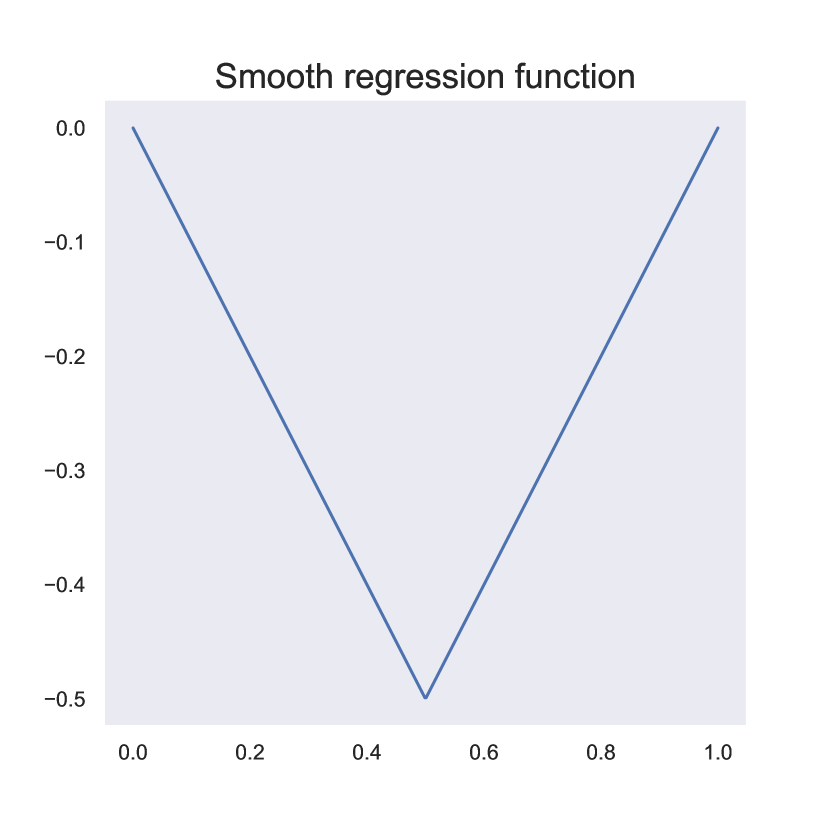
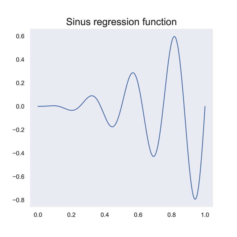
Figure 3: Smooth and sinus regression functions

5.3 Results of the simulation experiments

5.3.1 Finite-rank kernels

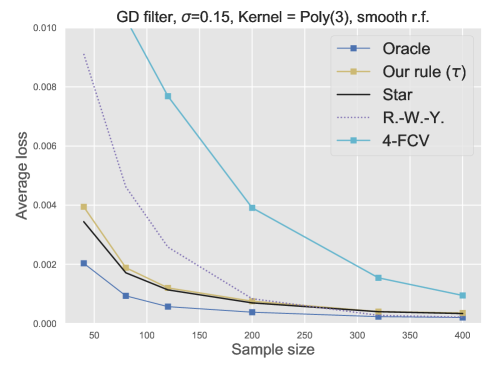
(a)

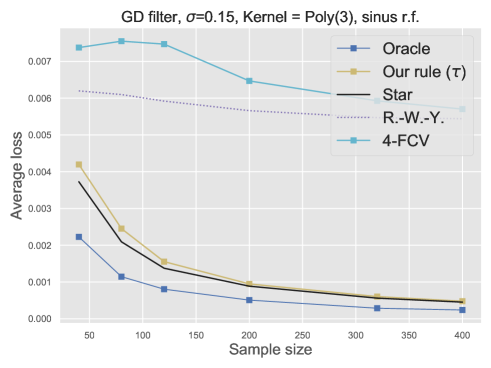
(b)

Figure 4: Kernel gradient descent with the step-size $\eta=1/(1.2\widehat{\mu}_{1})$ and polynomial kernel $\mathbb{K}(x_{1},x_{2})=(1+x_{1}^{\top}x_{2})^{3},\ x_{1},x_{2}\in[0,1]$, for the estimation of two noised regression functions from Figure 3: the smooth $f^{*}(x)=|x-1/2|-1/2$ for panel (a), and the ”sinus” $f^{*}(x)=0.9\ \textnormal{sin}(8\pi x)x^{2}$ for panel (b), with the equidistant covariates $x_{j}=j/n$. Each curve corresponds to the $L_{2}(\mathbb{P}_{n})$ squared norm error for the stopping rules (55), (23), (54), (53), (24) averaged over $100$ independent trials, versus the sample size $n=\{40,80,120,200,320,400\}$.

Figure 4 displays the (averaged) $L_{2}(\mathbb{P}_{n})$-norm error of the oracle stopping rule (55), our stopping rule $\tau$ (24), $t^{*}$ (23), minimax-optimal stopping rule $\widehat{\textnormal{T}}_{\textnormal{RWY}}$ (54), and $4$-fold cross validation stopping rule $\widehat{\textnormal{T}}_{\textnormal{VFCV}}$ (53) versus the sample size. Figure 4(a) shows the results for the piecewise linear regression function whereas Figure 4(b) corresponds to the ”sinus” regression function.

All the curves decrease as $n$ grows. From these graphs, the overall worst performance is achieved by $\widehat{\textnormal{T}}_{\textnormal{VFCV}}$, especially with a small sample size, which can be due to the additional randomness induced by the preliminary random splitting with $4-FCV$. By contrast, the minimum discrepancy-based stopping rules ($\tau$ and $t^{*}$) exhibit the best performances compared to the results of $\widehat{\textnormal{T}}_{\textnormal{VFCV}}$ and $\widehat{\textnormal{T}}_{\textnormal{RWY}}$. The averaged mean-squared error of $\tau$ is getting closer to the one of $t^{*}$ as the number of samples $n$ increases, which was expected from the theory and also intuitively, since $\tau$ has been introduced as an estimator of $t^{*}$. From Figure 4(a), $\widehat{\textnormal{T}}_{\textnormal{RWY}}$ is less accurate for small sample sizes, but improves a lot as $n$ grows up to achieving a performance similar to that of $\tau$. This can result from the fact that $\widehat{\textnormal{T}}_{\textnormal{RWY}}$ is built from upper bounds on the bias and variance terms, which are likely to be looser with a small sample size, but achieve an optimal convergence rate as $n$ increases. On Figure 4(b), the reason why $\tau$ exhibits (strongly) better results than $\widehat{\textnormal{T}}_{\textnormal{RWY}}$ owes to the main assumption on the regression function, namely that $\lVert f^{*}\rVert_{\mathcal{H}}\leq 1$. This could be violated for the ”sinus” function.

5.3.2 Polynomial eigenvalue decay kernels

Figure 5 displays the resulting (averaged over $100$ repetitions) $L_{2}(\mathbb{P}_{n})$-error of $\tau_{\alpha}$ (with $\alpha=\frac{1}{\beta+1}=0.33$) (37), $\widehat{\textnormal{T}}_{\textnormal{RWY}}$ (54), $t^{*}$ (23), and $\widehat{\textnormal{T}}_{\textnormal{HO}}$ (52) versus the sample size.

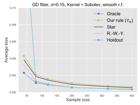
(a)

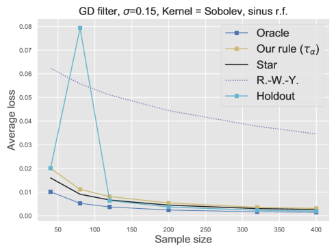
(b)

Figure 5: Kernel gradient descent (11) with the step-size $\eta=1/(1.2\widehat{\mu}_{1})$ and Sobolev kernel $\mathbb{K}(x_{1},x_{2})=\min\{x_{1},x_{2}\},\ x_{1},x_{2}\in[0,1]$ for the estimation of two noised regression functions from Figure 3: the smooth $f^{*}(x)=|x-1/2|-1/2$ for panel (a) and the ”sinus” $f^{*}(x)=0.9\ \textnormal{sin}(8\pi x)x^{2}$ for panel (b), with the equidistant covariates $x_{j}=j/n$. Each curve corresponds to the $L_{2}(\mathbb{P}_{n})$ squared norm error for the stopping rules (55), (23), (54), (52), (37) with $\alpha=0.33$, averaged over $100$ independent trials, versus the sample size $n=\{40,80,120,200,320,400\}$.

Figure 5(a) shows that all stopping rules seem to work equivalently well, although there is a slight advantage for $\widehat{\textnormal{T}}_{\textnormal{HO}}$ and $\widehat{\textnormal{T}}_{\textnormal{RWY}}$ compared to $t^{*}$ and $\tau_{\alpha}$. However, as $n$ grows to $n=400$, the performances of all stopping rules become very close to each other. Let us mention that the true value of $\beta$ is not known in these experiments. Therefore, the value $\frac{1}{\beta+1}=0.33$ has been estimated from the decay of the empirical eigenvalue of the normalized Gram matrix. This can explain why the performance of $\tau_{\alpha}$ remains worse than that of $\widehat{\textnormal{T}}_{\textnormal{RWY}}$.

The story described by Figure 5(b) is somewhat different. The first striking remark is that $\widehat{\textnormal{T}}_{\textnormal{RWY}}$ completely fails on this example, which still stems from the (unsatisfied) constraint on the $\mathcal{H}$-norm of $f^{*}$. However, the best performance is still achieved by the Hold-out stopping rule, although $\tau_{\alpha}$ and $t^{*}$ remain very close to the latter. The fact that $t^{*}$ remains close to the oracle stopping rule (without any need for smoothing) supports the idea that the minimum discrepancy is a reliable principle for designing an effective stopping rule. The deficiency of $\tau$ (by contrast to $\tau_{\alpha}$) then results from the variability of the empirical risk, which does not remain close enough to its expectation. This bad behavior is then balanced by introducing the polynomial smoothing at level $\alpha$ within the definition of $\tau_{\alpha}$, which enjoys close to optimal practical performances.

Let us also mention that $\widehat{\textnormal{T}}_{\textnormal{HO}}$ exhibit some variability, in particular, with small sample sizes as illustrated by Figures 5(a) and 5(b).

The overall conclusion is that the smoothed minimum discrepancy-based stopping rules $\tau_{\alpha}$ leads to almost optimal performances provided $\alpha=(\beta+1)^{-1}$, where $\beta$ quantifies the polynomial decay of the empirical eigenvalues of the normalized Gram matrix.

5.4 Estimation of variance and decay rate for polynomial eigenvalue decay kernels

The purpose of the present section is to describe two strategies for estimating: $(i)$ the decay rate of the empirical eigenvalues of the normalized Gram matrix, and $(ii)$ the variance parameter $\sigma^{2}$.

5.4.1 Polynomial decay parameter estimation

From the polynomial decay assumption (45), one easily derives upper and lower bounds for $\beta$ as

$$\frac{\log(\widehat{\mu}_{i}/\widehat{\mu}_{i+1})-\log(C/c)}{\log(1+1/i)}\leq\beta\leq\frac{\log(\widehat{\mu}_{i}/\widehat{\mu}_{i+1})+\log(C/c)}{\log(1+1/i)}.$$

The difference between these upper and lower bounds is equal to $\frac{2\log(C/c)}{\log(1+1/i)}$, which is minimized for $i=1$. Then the best precision on the estimated value of $\beta$ is reached with $i=1$, which yields the estimator

$$\widehat{\beta}=\frac{\log(\widehat{\mu}_{1}/\widehat{\mu}_{2})}{\log 2}.$$ (56)

Note that this estimator $\widehat{\beta}$ from (56) is not rigorously grounded but only serves as a rough choice in our simulation experiments (see Section  5.3).

5.4.2 Variance parameter estimation

There is a bunch of suggestions for variance estimation with linear smoothers; see, e.g., Section 5.6 in the book [Was06]. In our simulation experiments, two cases are distinguished: the situation where the reproducing kernel has finite rank $r$, and the situation where the empirical eigenvalues of the normalized Gram matrix exhibit a polynomial decay. In both cases, an asymptotically unbiased estimator of $\sigma^{2}$ is designed.

Finite-rank kernel.

With such a finite-rank kernel, the estimation of the noise is made from the coordinates $\{Z_{i}\}_{i=r+1}^{n}$ corresponding to the situation, where $G_{i}^{*}=0,\ i>r$ (see Lemma A.1 in Appendix A). Actually, these coordinates (which are pure noise) are exploited to build an easy-to-compute estimator of $\sigma^{2}$, that is,

$$\widehat{\sigma}^{2}=\frac{\sum_{i=n-r+1}^{n}Z_{i}^{2}}{n-r}.$$ (57)

Polynomial decay kernel.

If the empirical eigenvalues of $K_{n}$ satisfy the polynomial eigenvalue decay assumption (45), we suggest overly-smoothing the residuals by choosing $\alpha=1$, which intuitively results in reducing by a large amount the variability of the corresponding smoothed empirical risk around its expectation, that is, $\mathbb{E}_{\varepsilon}R_{1,t}\approx R_{1,t}$.

Therefore, the smoothed empirical risk can be approximated by $R_{1,t}\approx B_{1}^{2}(t)+\frac{\sigma^{2}}{n}\sum_{i=1}^{r}(1-\gamma_{i}^{(t)})^{2}$, and

$$\sigma^{2}\approx\frac{R_{1,t}-B_{1}^{2}(t)}{\frac{1}{n}\sum_{i=1}^{r}\widehat{\mu}_{i}(1-\gamma_{i}^{(t)})^{2}}.$$

Using furthermore that $B_{1}^{2}(t)\to 0$ as $t$ increases to $+\infty$, the final choice is

$$\widehat{\sigma}^{2}=\frac{R_{1,t}}{\frac{1}{n}\sum_{i=1}^{r}\widehat{\mu}_{i}(1-\gamma_{i}^{(t)})^{2}}.$$

Following the above heuristic argument, let us emphasize that $\widehat{\sigma}^{2}$ is likely to be an upper bound on the true variance $\sigma^{2}$ since the (non-negative) bias is lower bounded by 0. Nevertheless, the next result justifies this choice.

Lemma 5.1.

Under the polynomial eigenvalue decay assumption (45), any value of $t$ satisfying $t\cdot\eta\widehat{\epsilon}_{n}^{2}\to+\infty$ as $n\to+\infty$ yields that $\widehat{\sigma}^{2}=\frac{R_{1,t}}{\frac{1}{n}\sum_{i=1}^{r}\widehat{\mu}_{i}(1-\gamma_{i}^{(t)})^{2}}$ is an asymptotically unbiased estimator of $\sigma^{2}$.

A sketch of the proof of Lemma 5.1 is given in Appendix I. Based on this lemma, we suggest taking $t=T$, where $T$ is the maximum number of iterations allowed to execute due to computational constraints. Notice that as long as we access closed-form expressions of the estimator, there is no need to compute all estimators for $t$ between $1\leq t\leq T$. The final estimator of $\sigma^{2}$ used in the experiments of Section 5.3 is given by

$$\widehat{\sigma}^{2}=\frac{R_{1,T}}{\frac{1}{n}\sum_{i=1}^{r}\widehat{\mu}_{i}(1-\gamma_{i}^{(T)})^{2}}.$$ (58)

6 Conclusion

In this paper, we describe spectral filter estimators (gradient descent, kernel ridge regression) for the non-parametric regression function estimation in RKHS. Two new data-driven early stopping rules $\tau$ (24) and $\tau_{\alpha}$ (37) for these iterative algorithms are designed. In more detail, we show that for the infinite-rank reproducing kernels, $\tau$ has a high variance due to the variability of the empirical risk around its expectation, and we proposed a way to reduce this variability by means of smoothing the empirical $L_{2}(\mathbb{P}_{n})$-norm (and, as a consequence, the empirical risk) by the eigenvalues of the normalized kernel matrix. We demonstrate in Corollaries 3.5 and 4.4 that our stopping rules $\tau$ and $\tau_{\alpha}$ yield minimax-optimal rates, in particular, for finite-rank kernel classes and Sobolev spaces. It is worth to mention that computing our stopping rules (for a general reproducing kernel) requires only the estimation of the variance $\sigma^{2}$ and computing $(\widehat{\mu}_{1},\ldots,\widehat{\mu}_{r})$. Theoretical results are confirmed empirically: $\tau$ and $\tau_{\alpha}$ with the smoothing parameter $\alpha=\frac{1}{\beta+1}$, where $\beta$ is the polynomial decay rate of the eigenvalues of the normalized Gram matrix, perform favorably in comparison with stopping rules based on hold-out data and 4-fold cross-validation.

There are various open questions that could be tackled after our results. A deficiency of our strategy is that the construction of $\tau$ and $\tau_{\alpha}$ is based on the assumption that the regression function belongs to a known RKHS, which restricts (mildly) the smoothness of the regression function. We would like to understand how our results extend to other loss functions besides the squared loss (for example, in the classification framework), as it was done in [WYW17]. Another research direction could be to use early stopping with fast approximation techniques for kernels [Ang+15, RCR15] to avoid calculation of all eigenvalues of the normalized Gram matrix that can be prohibited for large-scale problems.

First, we provide a plan for Appendix to facilitate the reading.

In Appendix A, we state some results that are repeatedly used all along Appendix. Most of them are already known in the literature.

Appendix B establishes an upper bound on the $\alpha$-smoothed bias term and provides a deviation inequality for the variance term. These two results will be used throughout Appendix.

In Appendix C, we state an auxiliary lemma of minimax optimality of the stopping rule $t^{*}$ from Eq. (23). This lemma is used in the proof of Corollary 3.2.

The main goal of Appendix D is to provide auxiliary results for the proof of Theorem 4.1:

• Lemma D.1 $\longrightarrow$ decomposition of the risk error $\lVert f^{\tau_{\alpha}}-f^{*}\rVert_{n}^{2}$ that involves the following quantities:

  $$B^{2}(\tau_{\alpha})\textnormal{ and }v(\tau_{\alpha}),$$

  where $v(t)$ is the stochastic part of the variance at time $t$.

• Lemma D.2 $\longrightarrow$ the (right) deviation inequality for the stopping rule $\tau_{\alpha}$.

• Lemma D.3 $\longrightarrow$ the (left) deviation inequality for the stopping rule $\tau_{\alpha}$.

After that, Lemma D.2 and Lemma D.3 will be used in the following.

• Lemma D.4 will use Lemma D.2 to upper bound $v(\tau_{\alpha})$ with high probability.

• Lemma D.5 will use Lemma D.3 to upper bound $B^{2}(\tau_{\alpha})$ with high probability.

Further, we prove Theorem 4.1 in Appendix E by combining all the results from Appendix D.

In Appendix F, one can find the proof of Theorem 3.4. To be precise, in this proof, we can set $\alpha=0$ and use the same arguments as in Appendix E. This is the reason why Appendix F follows Appendix E.

Appendix G establishes an explicit expression for the smoothed Rademacher compexity $\widehat{R}_{n,\alpha}(\epsilon,\mathcal{H})$.

We collect all the remaining auxiliary lemmas in Appendix H. A sketch of the proof of Lemma 5.1 is in Appendix I.

Appendix A Useful results

In this section, we present several auxiliary lemmas that are repeatedly used along the paper.

The first one provides a result showing that we have some coordinates of $G^{*}$ equal to zero when we transform the initial model (5) to its rotated version (8).

Lemma A.1.

[RWY14, Section 4.1.1] If $f^{*}\in\mathcal{H}$ with a bounded kernel $\mathbb{K}$ and Gram matrix $K=\mathbb{K}(x_{i},x_{j}),\ i,j=1,\ldots,n$ such that $rk(K)=r\leq n$, then

$$G_{i}^{*}=\langle\widehat{u}_{i},F^{*}\rangle=0\text{ when }i>r.$$ (59)

The following auxiliary lemma plays a crucial role in all proofs. It provides a sharp control of the spectral filter function defined in (11).

Lemma A.2.

[RWY14, Lemmas 8 and Section 4.1.1] For any bounded kernel, with $\gamma_{i}^{(t)}$ corresponding to gradient descent or kernel ridge regression, for every $t>0$,

$$\frac{1}{2}\min\{1,\eta t\widehat{\mu}_{i}\}\leq\gamma_{i}^{(t)}\leq\min\{1,\eta t\widehat{\mu}_{i}\},\ \ i=1,\ldots,n,$$ (60)

$$\frac{1}{n}\sum_{i=1}^{r}\frac{(G_{i}^{*})^{2}}{\widehat{\mu}_{i}}\leq R^{2},\quad\textnormal{and}\quad B^{2}(t)\leq\frac{R^{2}}{\eta t}.$$ (61)

Lemma A.3 establishes the magnitude of the population critical radius $\epsilon_{n}$ for different kernel spaces.

Lemma A.3.

[RWY14, Section 4.3] Recall the definitions of the localized population Rademacher complexity (29) and its population critical radius $\epsilon_{n}$ (30), then

• for finite-rank kernels with rank $r$,

  $$\epsilon_{n}^{2}=c_{1}\frac{r\sigma^{2}}{nR^{2}},$$

  for a positive numeric constant $c_{1}>0$.

• for polynomial eigenvalue decay kernels $\mu_{i}\leq C_{\mu}i^{-\beta}$,

  $$\epsilon_{n}^{2}\asymp\left[\frac{\sigma^{2}}{2R^{2}n}\left[1+\sqrt{\frac{C_{\mu}}{\beta-1}}\right]^{2}\right]^{\frac{\beta}{\beta+1}}.$$ (62)

Lemma A.4 establishes the magnitude of the empirical critical radius $\widehat{\epsilon}_{n}$ for different kernel spaces.

Lemma A.4.

Recall the definitions of the empirical localized Rademacher complexity (19) and its critical radius (20). Then

• for finite-rank kernels with rank $r$,

  $$\widehat{\epsilon}_{n}^{2}=c\frac{\sigma^{2}r}{nR^{2}}\ \ \textnormal{ for a positive numeric constant }c.$$

• for polynomial eigenvalue decay kernels (45) with eigenvalue decay $\beta>1$,

  $$\widehat{\epsilon}_{n}^{2}\asymp\left[1+\sqrt{\frac{C}{\beta-1}}\right]^{\frac{2\beta}{\beta+1}}\left[\frac{\sigma^{2}}{2nR^{2}}\right]^{\frac{\beta}{\beta+1}}.$$

Proof of Lemma A.4.

The bounds for the finite-rank and polynomial-eigendecay kernels could be derived in the same manner as in the proof of Lemma A.3, using the upper bound on the eigenvalues $\widehat{\mu}_{i}\leq Ci^{-\beta},i=1,\ldots,r$. ∎

The following result shows the magnitude of the smoothed critical radius defined in Ineq. (41) for polynomial eigenvalue decay kernels.

Lemma A.5.

Under the assumption $\widehat{\mu}_{i}\leq Ci^{-\beta},\ i\in[r]$, for $\alpha\beta<1$, one has

$$\widehat{\epsilon}_{n,\alpha}^{2}\asymp\left[\sqrt{\frac{C^{\alpha}}{1-\alpha\beta}}+\sqrt{\frac{C^{1+\alpha}}{\beta(1+\alpha)-1}}\right]^{\frac{2\beta}{\beta+1}}\left[\frac{\sigma^{2}}{2R^{2}n}\right]^{\frac{\beta}{\beta+1}}.$$

Proof of Lemma A.5.

For every $M\in(0,r]$ and $\alpha\beta<1$, we have

$$\widehat{\mathcal{R}}_{n,\alpha}(\epsilon,\mathcal{H}) \leq R\sqrt{\frac{1}{n}}\sqrt{\sum_{j=1}^{r}\min\{Cj^{-\beta},\epsilon^{2}\}C^{\alpha}j^{-\beta\alpha}}$$

$$\leq R\sqrt{\frac{C^{\alpha}}{n}}\sqrt{\sum_{j=1}^{\left\lfloor M\right\rfloor}j^{-\beta\alpha}}\epsilon+R\sqrt{\frac{C^{1+\alpha}}{n}}\sqrt{\sum_{j=\left\lceil M\right\rceil}^{n}j^{-\beta-\beta\alpha}}$$

$$\leq R\sqrt{\frac{C^{\alpha}}{1-\alpha\beta}\frac{M^{1-\alpha\beta}}{n}}\epsilon+R\sqrt{\frac{C^{1+\alpha}}{n}}\sqrt{\frac{1}{\beta(1+\alpha)-1}\frac{1}{M^{\beta(1+\alpha)-1}}}.$$

Set $M=\epsilon^{-2/\beta}$ that implies $\sqrt{M^{1-\alpha\beta}}\epsilon=\epsilon^{1-\frac{1-\alpha\beta}{\beta}}$, and

$$\widehat{\mathcal{R}}_{n,\alpha}(\epsilon,\mathcal{H})\leq R\left[\sqrt{\frac{C^{\alpha}}{1-\alpha\beta}}+\sqrt{\frac{C^{1+\alpha}}{\beta(1+\alpha)-1}}\right]\epsilon^{1-\frac{1-\alpha\beta}{\beta}}\frac{1}{\sqrt{n}}.$$

Therefore, the smoothed critical inequality $\widehat{\mathcal{R}}_{n,\alpha}(\epsilon,\mathcal{H})\leq\frac{2R^{2}}{\sigma}\epsilon^{2+\alpha}$ is satisfied for

$$\widehat{\epsilon}_{n,\alpha}^{2}\asymp\left[\sqrt{\frac{C^{\alpha}}{1-\alpha\beta}}+\sqrt{\frac{C^{1+\alpha}}{\beta(1+\alpha)-1}}\right]^{\frac{2\beta}{\beta+1}}\left[\frac{\sigma^{2}}{2R^{2}n}\right]^{\frac{\beta}{\beta+1}}.$$

∎

In order to transfer the $L_{2}(\mathbb{P}_{n})$-norm into the $L_{2}(\mathbb{P}_{X})$-norm, we need to relate the empirical critical radius $\widehat{\epsilon}_{n}$ with its population counterpart $\epsilon_{n}$. It is achieved by the following result.

Lemma A.6.

There are numeric constants $c_{1},c_{2},c_{3},c_{4}>0$ such that $c_{1}\epsilon_{n}\leq\widehat{\epsilon}_{n}\leq c_{2}\epsilon_{n}$ with probability at least $1-c_{3}\exp\Big{(}-c_{4}\frac{R^{2}}{\sigma^{2}}n\epsilon_{n}^{2}\Big{)}$.

Sketch of the proof of Lemma A.6.

The claim follows from known results on empirical processes and RKHS (see, e.g., Theorem 14.1 and the discussion afterwards in [Wai19]). ∎

Appendix B Handling the smoothed bias and variance

B.1 Upper bound on the smoothed bias

The first lemma provides an upper bound on the smoothed bias term.

Lemma B.1.

Under Assumptions 1, 2,

$$B_{\alpha}^{2}(t)\leq\frac{R^{2}}{(\eta t)^{1+\alpha}},\quad\alpha\in[0,1].$$ (63)

Proof of Lemma B.1.

For any $t>0$,

$$B_{\alpha}^{2}(t)=\frac{1}{n}\sum_{i=1}^{r}\widehat{\mu}_{i}^{\alpha}(1-\gamma_{i}^{(t)})^{2}(G_{i}^{*})^{2} \leq\frac{1}{n}\sum_{i=1}^{r}\widehat{\mu}_{i}^{\alpha}(1-\gamma_{i}^{(t)})^{1+\alpha}(G_{i}^{*})^{2}$$

$$\overset{(\textnormal{i})}{\leq}\frac{1}{n(\eta t)^{1+\alpha}}\sum_{i=1}^{r}\frac{(G_{i}^{*})^{2}}{\widehat{\mu}_{i}}$$

$$\overset{(\textnormal{ii})}{\leq}\frac{R^{2}}{(\eta t)^{1+\alpha}}.$$

(i) is true thanks to the qualification condition (10) with $\overline{\nu}=1$, (ii) is due to the bounds in (61). ∎

B.2 Deviation inequality for the variance term

In this subsection, we recall one concentration result from [RWY14, Section 4.1.2].

For any $t>0$, define a matrix $Q_{t}\coloneqq\textnormal{diag}\{(\gamma_{j}^{(t)})^{2},\ j\in[r]\}$, then one concludes that $V(t)=\mathbb{E}_{\varepsilon}[v(t)]=\frac{\sigma^{2}}{n}\textnormal{tr}[Q_{t}]$. After that, since $\gamma_{i}^{(t)}\leq\min\{1,\eta t\widehat{\mu}_{i}\}$ for $i\in[r]$,

$$V(t)=\frac{\sigma^{2}}{n}\textnormal{tr}[Q_{t}]\leq\frac{\sigma^{2}}{n}\sum_{j=1}^{r}\min\{1,\eta t\widehat{\mu}_{i}\}=\frac{\sigma^{2}\eta t}{R^{2}}\widehat{\mathcal{R}}_{n}^{2}\left(\frac{1}{\sqrt{\eta t}},\mathcal{H}\right).$$ (64)

Consider a random variable of the form $\widetilde{Q}_{n}=\sum_{i,j=1}^{n}a_{ij}Z_{i}Z_{j}$, where $\{Z_{i}\}_{i=1}^{n}$ are zero-mean Gaussian r.v. with parameter $\sigma$. Then, [RV+13] proved that

$$\mathbb{P}_{\varepsilon}\left(|\widetilde{Q}_{n}-\mathbb{E}_{\varepsilon}[\widetilde{Q}_{n}]|\geq\delta\right)\leq 2\ \exp\left[-c\min\left\{\frac{\delta}{\sigma^{2}\lVert A\rVert_{\textnormal{op}}},\frac{\delta^{2}}{\sigma^{4}\lVert A\rVert_{F}^{2}}\right\}\right]\ \forall\delta>0,$$ (65)

where $\lVert A\rVert_{\textnormal{op}}$ and $\lVert A\rVert_{F}$ are the operator and Frobenius norms of the matrix $A=\{a_{ij}\}_{i,j=1}^{n}$, respectively.

By applying Ineq. (65) with $A=\frac{1}{n}Q_{t}$, $Z_{i}=\varepsilon_{i},\ i\in[r],$ it yields $\widetilde{Q}_{n}=v(t)$, and

$$\begin{split}\lVert A\rVert_{\textnormal{op}}&\leq\frac{1}{n},\\ \lVert A\rVert_{F}^{2}=\frac{1}{n^{2}}\textnormal{tr}[Q_{t}^{2}]&\leq\frac{1}{n^{2}}\textnormal{tr}[Q_{t}]\leq\frac{\eta t}{nR^{2}}\widehat{\mathcal{R}}_{n}^{2}\left(\frac{1}{\sqrt{\eta t}},\mathcal{H}\right).\end{split}$$ (66)

Consequently, for any $t>0$ and $\delta>0$, one gets

$$\mathbb{P}_{\varepsilon}\Big{(}|v(t)-V(t)|\geq\delta\Big{)}\leq 2\ \exp\left[-\frac{cn\delta}{\sigma^{2}}\min\left\{1,\frac{R^{2}\delta}{\sigma^{2}\eta t\widehat{\mathcal{R}}_{n}^{2}(\frac{1}{\sqrt{\eta t}},\mathcal{H})}\right\}\right].$$ (67)

Let us first transfer the critical inequality (20) from $\epsilon$ to $t$.

Definition B.1.

Set $\epsilon=\frac{1}{\sqrt{\eta t}}$ in (20), and let us define $\widehat{t}_{\epsilon}$ as the largest positive solution to the following fixed-point equation

$$\frac{\sigma^{2}\eta t}{R^{2}}\widehat{\mathcal{R}}_{n}^{2}\left(\frac{1}{\sqrt{\eta t}},\mathcal{H}\right)\leq\frac{4R^{2}}{\eta t}.$$ (68)

Note that in Lemma A.4, the empirical critical radius $\widehat{\epsilon}_{n}=\frac{1}{\sqrt{\eta\widehat{t}_{\epsilon}}}$, and such a point $\widehat{t}_{\epsilon}$ exists since $\widehat{\epsilon}_{n}$ exists and is unique [Men02, BBM+05, RWY14]. Moreover, $\widehat{t}_{\epsilon}$ provides the equality in Ineq. (68).

Appendix C Auxiliary lemma for finite-rank kernels

Remark that at $t=t^{*}:B^{2}(t)=\frac{2\sigma^{2}}{n}\sum_{i=1}^{r}\gamma_{i}^{(t)}-V(t)\geq\frac{\sigma^{2}}{n}\sum_{i=1}^{r}\gamma_{i}^{(t)}$. Thus, due to the construction of $\widehat{t}_{\epsilon}$ ( $\widehat{t}_{\epsilon}$ is the point of intersection of an upper bound on the bias and a lower bound on $\frac{\sigma^{2}}{2n}\sum_{i=1}^{r}\gamma_{i}^{(t)}$) and monotonicity (in $t$) of all the terms involved, we get $t^{*}\leq\widehat{t}_{\epsilon}$.

Lemma C.1.

Recall the definition of the stopping rule $t^{*}$ (23). Under Assumptions 1, 2, and 3, for the gradient descent/kernel ridge regression filter, the following holds for any reproducing kernel:

$$\mathbb{E}_{\varepsilon}\lVert f^{t^{*}}-f^{*}\rVert_{n}^{2}\leq 8R^{2}\widehat{\epsilon}_{n}^{2}.$$

Proof of Lemma C.1.

Let us define a proxy version of the variance term: $\widetilde{V}(t)\coloneqq\frac{\sigma^{2}}{n}\sum_{i=1}^{r}\gamma_{i}^{(t)}$. Moreover, for all $t>0$,

$$\mathbb{E}_{\varepsilon}R_{t}=B^{2}(t)+\frac{\sigma^{2}}{n}\sum_{i=1}^{n}(1-\gamma_{i}^{(t)})^{2}.$$ (69)

From the fact that $\mathbb{E}_{\varepsilon}R_{t^{*}}=\sigma^{2}$,

$$\mathbb{E}_{\varepsilon}\lVert f^{t^{*}}-f^{*}\rVert_{n}^{2}=B^{2}(t^{*})+V(t^{*})=2\widetilde{V}(t^{*}).$$ (70)

Therefore, in order to prove the lemma, our goal is to get an upper bound on $\widetilde{V}(t^{*})$.

Since the function $\eta t\widehat{\mathcal{R}}_{n}^{2}(\frac{1}{\sqrt{\eta t}},\mathcal{H})$ is monotonic in $t$ (see, for example, Lemma H.1), and $t^{*}\leq\widehat{t}_{\epsilon}$, we conclude that

$$\widetilde{V}(t^{*})\leq\frac{\sigma^{2}\eta t^{*}}{R^{2}}\widehat{\mathcal{R}}_{n}^{2}\left(\frac{1}{\sqrt{\eta t^{*}}},\mathcal{H}\right)\leq\frac{\sigma^{2}\eta\widehat{t}_{\epsilon}}{R^{2}}\widehat{\mathcal{R}}_{n}^{2}\left(\frac{1}{\sqrt{\eta\widehat{t}_{\epsilon}}},\mathcal{H}\right)=4R^{2}\widehat{\epsilon}_{n}^{2}.$$

∎

Appendix D Proofs for polynomial smoothing

In the proofs, we will need three additional definitions below.

Definition D.1.

In Definition 4.2, set $\epsilon=\frac{1}{\sqrt{\eta t}}$, then for any $\alpha\in[0,1]$, the smoothed critical inequality (41) is equivalent to

$$\frac{\sigma^{2}\eta t}{4}\widehat{\mathcal{R}}_{n,\alpha}^{2}\Big{(}\frac{1}{\sqrt{\eta t}},\mathcal{H}\Big{)}\leq\frac{R^{4}}{(\eta t)^{1+\alpha}}.$$ (71)

Due to Lemma H.1, the left-hand side of (71) is non-decreasing in $t$, and the right-hand side is non-increasing in $t$.

Definition D.2.

For any $\alpha\in[0,1]$, define the stopping rule $\widehat{t}_{\epsilon,\alpha}$ such that

$$\widehat{\epsilon}_{n,\alpha}^{2}=\frac{1}{\eta\widehat{t}_{\epsilon,\alpha}},$$ (72)

then Ineq. (71) becomes the equality at $t=\widehat{t}_{\epsilon,\alpha}$ thanks to the monotonicity and continuity of both terms in the inequality.

Further, we define the stopping rules $\widetilde{t}_{\epsilon,\alpha}$ and $\overline{t}_{\epsilon,\alpha}$ that will serve as a lower bound and an upper bound on $t_{\alpha}^{*}$ for all $\alpha\in[0,1]$.

Definition D.3.

Define the smoothed proxy variance $\widetilde{V}_{\alpha}(t)\coloneqq\frac{\sigma^{2}}{n}\sum_{i=1}^{r}\widehat{\mu}_{i}^{\alpha}\gamma_{i}^{(t)}$ and the following stopping rules

$$\begin{split}\overline{t}_{\epsilon,\alpha}&=\inf\big{\{}t>0\ |\ B_{\alpha}^{2}(t)=\frac{1}{2}\widetilde{V}_{\alpha}(t)\big{\}},\\ \widetilde{t}_{\epsilon,\alpha}&=\inf\big{\{}t>0\ |\ B_{\alpha}^{2}(t)=3\widetilde{V}_{\alpha}(t)\big{\}}.\end{split}$$ (73)

Notice that at $t=\widetilde{t}_{\epsilon,\alpha}$:

$$\frac{6R^{2}}{(\eta t)^{1+\alpha}}\geq\frac{R^{2}}{(\eta t)^{1+\alpha}}\geq B_{\alpha}^{2}(t)=3\widetilde{V}_{\alpha}(t)\geq\frac{3}{2}\frac{\sigma^{2}}{R^{2}}\eta t\widehat{\mathcal{R}}_{n,\alpha}^{2}\Big{(}\frac{1}{\sqrt{\eta t}},\mathcal{H}\Big{)}.$$

At $t=\overline{t}_{\epsilon,\alpha}$:

$$\frac{R^{2}}{(\eta t)^{1+\alpha}}\geq B_{\alpha}^{2}(t)=\frac{1}{2}\widetilde{V}_{\alpha}(t)\geq\frac{\sigma^{2}\eta t}{4R^{2}}\widehat{\mathcal{R}}_{n,\alpha}^{2}\Big{(}\frac{1}{\sqrt{\eta t}},\mathcal{H}\Big{)}.$$

Thus, $\widetilde{t}_{\epsilon,\alpha}$ and $\overline{t}_{\epsilon,\alpha}$ satisfy the smoothed critical inequality (71). Moreover, $\widehat{t}_{\epsilon,\alpha}$ is always greater than or equal to $\overline{t}_{\epsilon,\alpha}$ and $\widetilde{t}_{\epsilon,\alpha}$ since $\widehat{t}_{\epsilon,\alpha}$ is the largest value satisfying Ineq. (71). As a consequence of Lemma H.1, one has

$$\frac{1}{\eta\widetilde{t}_{\epsilon,\alpha}}\asymp\frac{1}{\eta\overline{t}_{\epsilon,\alpha}}\asymp\frac{1}{\eta\widehat{t}_{\epsilon,\alpha}}=\widehat{\epsilon}_{n,\alpha}^{2}.$$

Assume for simplicity that

$$\overline{\epsilon}_{n,\alpha}^{2} \coloneqq\frac{1}{\eta\overline{t}_{\epsilon,\alpha}}=c^{\prime}\frac{1}{\eta\widehat{t}_{\epsilon,\alpha}}=c^{\prime}\widehat{\epsilon}_{n,\alpha}^{2},$$

$$\widetilde{\epsilon}_{n,\alpha}^{2} \coloneqq\frac{1}{\eta\widetilde{t}_{\epsilon,\alpha}}=c^{\prime\prime}\frac{1}{\eta\widehat{t}_{\epsilon,\alpha}}=c^{\prime\prime}\widehat{\epsilon}_{n,\alpha}^{2}$$

for some positive numeric constants $c^{\prime},c^{\prime\prime}\geq 1$, due to the fact that $\widehat{t}_{\epsilon,\alpha}\geq\overline{t}_{\epsilon,\alpha}$ and $\widehat{t}_{\epsilon,\alpha}\geq\widetilde{t}_{\epsilon,\alpha}$.

The following lemma decomposes the risk error into several parts that will be further analyzed in subsequent Lemmas D.4, D.5.

Lemma D.1.

Recall the definition of $\tau_{\alpha}$ (37), then

$$\lVert f^{\tau_{\alpha}}-f^{*}\rVert_{n}^{2}\leq 2B^{2}(\tau_{\alpha})+2v(\tau_{\alpha}),$$

where $v(t)=\frac{1}{n}\sum_{i=1}^{n}(\gamma_{i}^{(t)})^{2}\varepsilon_{i}^{2},\ t>0$, is the stochastic part of the variance.

Proof of Lemma D.1.

Recall Definition 2.1 of the spectral filter function $g_{\lambda_{t}}(\xi)\equiv g_{t}(\xi).$

Let us define the noise vector $\varepsilon\coloneqq[\varepsilon_{1},...,\varepsilon_{n}]^{\top}$ and, for each $t>0$, two vectors that correspond to the bias and variance parts, respectively:

$$\tilde{b}^{2}(t) \coloneqq(g_{t}(K_{n})K_{n}-I_{n})F^{*},$$

$$\tilde{v}(t) \coloneqq g_{t}(K_{n})K_{n}\varepsilon.$$

This gives the following expressions for the stochastic part of the variance and bias:

$$v(t)=\langle\tilde{v}(t),\tilde{v}(t)\rangle_{n},\ \ B^{2}(t)=\langle\tilde{b}^{2}(t),\tilde{b}^{2}(t)\rangle_{n}.$$ (74)

General expression for the $L_{2}(\mathbb{P}_{n})$-norm error at $\tau_{\alpha}$ takes the form

$$\lVert f^{\tau_{\alpha}}-f^{*}\rVert_{n}^{2}=B^{2}(\tau_{\alpha})+v(\tau_{\alpha})+2\langle\tilde{b}^{2}(\tau_{\alpha}),\tilde{v}(\tau_{\alpha})\rangle_{n}.$$ (75)

Therefore, applying the inequality $2\left|\langle x,y\rangle_{n}\right|\leq\lVert x\rVert_{n}^{2}+\lVert y\rVert_{n}^{2}$ for any $x,y\in\mathbb{R}^{n}$, and (74), we obtain

$$\lVert f^{\tau_{\alpha}}-f^{*}\rVert_{n}^{2}\leq 2B^{2}(\tau_{\alpha})+2v(\tau_{\alpha}).$$ (76)

∎

D.1 Two deviation inequalities for $\tau_{\alpha}$

This is the first deviation inequality for $\tau_{\alpha}$ that will be further used in Lemma D.4 to control the variance term.

Lemma D.2.

Recall Definition D.3 of $\overline{t}_{\epsilon,\alpha}$, then under Assumptions 1, 2, 3, and 5,

$$\mathbb{P}_{\varepsilon}\Big{(}\tau_{\alpha}>\overline{t}_{\epsilon,\alpha}\Big{)}\leq 2\ \exp\left[-c_{1}\frac{R^{2}}{\sigma^{2}}n\widehat{\epsilon}_{n,\alpha}^{2(1+\alpha)}\right],$$

where a positive constant $c_{1}$ depends only on $\mathcal{M}$.

Proof of Lemma D.2.

Set $\kappa_{\alpha}\coloneqq\sigma^{2}\textnormal{tr}K_{n}^{\alpha}/n$, then due to the monotonicity of the smoothed empirical risk, for all $t\geq t_{\alpha}^{*}$,

$$\mathbb{P}_{\varepsilon}\left(\tau_{\alpha}>t\right)=\mathbb{P}_{\varepsilon}\left(R_{\alpha,t}-\mathbb{E}_{\varepsilon}R_{\alpha,t}>\kappa_{\alpha}-\mathbb{E}_{\varepsilon}R_{\alpha,t}\right).$$

Consider

$$R_{\alpha,t}-\mathbb{E}_{\varepsilon}R_{\alpha,t}=\underbrace{\frac{\sigma^{2}}{n}\sum_{i=1}^{r}\widehat{\mu}_{i}^{\alpha}(1-\gamma_{i}^{(t)})^{2}\left(\frac{\varepsilon_{i}^{2}}{\sigma^{2}}-1\right)}_{\Sigma_{1}}+\underbrace{\frac{2}{n}\sum_{i=1}^{r}\widehat{\mu}_{i}^{\alpha}(1-\gamma_{i}^{(t)})^{2}G_{i}^{*}\varepsilon_{i}}_{\Sigma_{2}}.$$ (77)

Define

$$\Delta_{t,\alpha}\coloneqq\kappa_{\alpha}-\mathbb{E}_{\varepsilon}R_{\alpha,t}=-B_{\alpha}^{2}(t)-V_{\alpha}(t)+2\widetilde{V}_{\alpha}(t),$$

where $\widetilde{V}_{\alpha}(t)=\frac{\sigma^{2}}{n}\sum_{i=1}^{r}\widehat{\mu}_{i}^{\alpha}\gamma_{i}^{(t)}$.

Further, set $t=\overline{t}_{\epsilon,\alpha}$, and recall that $\eta\overline{t}_{\epsilon,\alpha}=\frac{\eta\widehat{t}_{\epsilon,\alpha}}{c^{\prime}}$ for $c^{\prime}\geq 1$. This implies

$$\Delta_{\overline{t}_{\epsilon,\alpha},\alpha}\geq\frac{1}{2}\widetilde{V}_{\alpha}(\overline{t}_{\epsilon,\alpha}) \geq\frac{\sigma^{2}}{4n}\sum_{i=1}^{r}\widehat{\mu}_{i}^{\alpha}\min\left\{1,\frac{\eta\widehat{t}_{\epsilon,\alpha}}{c^{\prime}}\widehat{\mu}_{i}\right\}$$

$$=\frac{\sigma^{2}\eta\widehat{t}_{\epsilon,\alpha}}{4nc^{\prime}}\sum_{i=1}^{r}\widehat{\mu}_{i}^{\alpha}\min\left\{\frac{c^{\prime}}{\eta\widehat{t}_{\epsilon,\alpha}},\widehat{\mu}_{i}\right\}$$

$$\geq\frac{\sigma^{2}\eta\widehat{t}_{\epsilon,\alpha}}{4c^{\prime}R^{2}}\widehat{\mathcal{R}}_{n,\alpha}^{2}\left(\frac{1}{\sqrt{\eta\widehat{t}_{\epsilon,\alpha}}},\mathcal{H}\right)$$

$$=\frac{R^{2}}{c^{\prime}}\widehat{\epsilon}_{n,\alpha}^{2(1+\alpha)}.$$

Then, by standard concentration results on linear and quadratic sums of Gaussian random variables (see, e.g., [BHR16, Lemma 6.1]),

$$\mathbb{P}_{\varepsilon}\left(\Sigma_{1}>\frac{\Delta_{\overline{t}_{\epsilon,\alpha},\alpha}}{2}\right) \leq\exp\left[-\frac{\Delta_{\overline{t}_{\epsilon,\alpha},\alpha}^{2}}{16(\lVert a(\overline{t}_{\epsilon,\alpha})\rVert^{2}+\frac{\Delta_{\overline{t}_{\epsilon,\alpha},\alpha}}{2}\lVert a(\overline{t}_{\epsilon,\alpha})\rVert_{\infty})}\right],$$ (78)

$$\mathbb{P}_{\varepsilon}\left(\Sigma_{2}>\frac{\Delta_{\overline{t}_{\epsilon,\alpha},\alpha}}{2}\right) \leq\exp\left[-\frac{n\Delta_{\overline{t}_{\epsilon,\alpha},\alpha}^{2}}{32\sigma^{2}B_{\alpha}^{2}(\overline{t}_{\epsilon,\alpha})}\right],$$ (79)

where $a_{i}(\overline{t}_{\epsilon,\alpha})=\frac{\sigma^{2}}{n}\widehat{\mu}_{i}^{\alpha}(1-\gamma_{i}^{(\overline{t}_{\epsilon,\alpha})})^{2},\ i\in[r]$.

In what follows, we simplify the bounds above.

Firstly, recall that $B=1$, which implies $\widehat{\mu}_{1}\leq 1$, and $\lVert a(\overline{t}_{\epsilon,\alpha})\rVert_{\infty}=\underset{i\in[r]}{\max}|a_{i}(\overline{t}_{\epsilon,\alpha})|\leq\frac{\sigma^{2}}{n}$, and

$$\frac{1}{2}\Delta_{\overline{t}_{\epsilon,\alpha},\alpha}\leq\frac{3}{4}\widetilde{V}_{\alpha}(\overline{t}_{\epsilon,\alpha})\leq\frac{3}{4}\widetilde{V}_{\alpha}(\widehat{t}_{\epsilon,\alpha}) \leq\frac{3}{4R^{2}}\sigma^{2}\eta\widehat{t}_{\epsilon,\alpha}\widehat{\mathcal{R}}_{n,\alpha}^{2}\left(\frac{1}{\sqrt{\eta\widehat{t}_{\epsilon,\alpha}}},\mathcal{H}\right)$$

$$=3R^{2}\widehat{\epsilon}_{n,\alpha}^{2(1+\alpha)}.$$

Secondly, we will upper bound the Euclidean norm of $a(\overline{t}_{\epsilon,\alpha})$. Recall Assumption 5, the definition of the smoothed statistical dimension $d_{n,\alpha}=\min\{j\in[r]:\widehat{\mu}_{j}\leq\widehat{\epsilon}_{n,\alpha}^{2}\}$, and Ineq. (43): $\widehat{\epsilon}_{n,\alpha}^{2(1+\alpha)}\geq\frac{\sigma^{2}\sum_{i=1}^{d_{n,\alpha}}\widehat{\mu}_{i}^{\alpha}}{4R^{2}n}$, which implies

$$\lVert a(\overline{t}_{\epsilon,\alpha})\rVert^{2}=\frac{\sigma^{4}}{n^{2}}\sum_{i=1}^{r}\widehat{\mu}_{i}^{2\alpha}(1-\gamma_{i}^{(\overline{t}_{\epsilon,\alpha})})^{4} \leq\frac{\sigma^{4}}{n^{2}}\left[\sum_{i=1}^{d_{n,\alpha}}\widehat{\mu}_{i}^{\alpha}+\sum_{i=d_{n,\alpha}+1}^{r}\widehat{\mu}_{i}^{2\alpha}\right]$$

$$\leq\frac{\sigma^{4}}{n^{2}}\left[\frac{4nR^{2}\widehat{\epsilon}_{n,\alpha}^{2(1+\alpha)}}{\sigma^{2}}+\mathcal{M}\sum_{i=1}^{d_{n,\alpha}}\widehat{\mu}_{i}^{\alpha}\right]$$

$$\leq\frac{4\sigma^{2}}{n}\left(1+\mathcal{M}\right)R^{2}\widehat{\epsilon}_{n,\alpha}^{2(1+\alpha)}.$$

Finally, using the upper bound $B_{\alpha}^{2}(\overline{t}_{\epsilon,\alpha})\leq\frac{R^{2}}{(\eta\overline{t}_{\epsilon,\alpha})^{1+\alpha}}\leq R^{2}(c^{\prime})^{2}\widehat{\epsilon}_{n,\alpha}^{2(1+\alpha)}$ for all $\alpha\in[0,1]$, one gets

$$\mathbb{P}_{\varepsilon}\left(\tau_{\alpha}>\overline{t}_{\epsilon,\alpha}\right)\leq 2\ \exp\left[-c_{1}\frac{R^{2}}{\sigma^{2}}n\widehat{\epsilon}_{n,\alpha}^{2(1+\alpha)}\right],$$ (80)

for some positive numeric $c_{1}>0$ that depends only on $\mathcal{M}$.

∎

What follows is the second deviation inequality for $\tau_{\alpha}$ that will be further used in Lemma D.5 to control the bias term.

Lemma D.3.

Recall Definition D.3 of $\widetilde{t}_{\epsilon,\alpha}$, then under Assumptions 1, 2, 3, and 5,

$$\mathbb{P}_{\varepsilon}\left(\tau_{\alpha}<\widetilde{t}_{\epsilon,\alpha}\right)\leq 2\ \exp\left[-c_{2}\frac{R^{2}}{\sigma^{2}}n\widehat{\epsilon}_{n,\alpha}^{2(1+\alpha)}\right]$$ (81)

for a positive constant $c_{2}$ that depends only on $\mathcal{M}$.

Proof of Lemma D.3.

Set $\kappa_{\alpha}\coloneqq\sigma^{2}\textnormal{tr}K_{n}^{\alpha}/n$. Note that $\widetilde{t}_{\epsilon,\alpha}\leq t_{\alpha}^{*}$ by construction.

Further, for all $t\leq t_{\alpha}^{*}$, due to the monotonicity of the smoothed empirical risk,

$$\mathbb{P}_{\varepsilon}\Big{(}\tau_{\alpha}<t\Big{)} =\mathbb{P}_{\varepsilon}\Big{(}R_{\alpha,t}-\mathbb{E}_{\varepsilon}R_{\alpha,t}\leq-(\mathbb{E}_{\varepsilon}R_{\alpha,t}-\kappa_{\alpha})\Big{)}$$

$$\leq\mathbb{P}_{\varepsilon}\bigg{(}\underbrace{\frac{\sigma^{2}}{n}\sum_{i=1}^{r}\widehat{\mu}_{i}^{\alpha}(1-\gamma_{i}^{(t)})^{2}\Big{(}\frac{\varepsilon_{i}^{2}}{\sigma^{2}}-1\Big{)}}_{\Sigma_{1}}\leq-\frac{\mathbb{E}_{\varepsilon}R_{\alpha,t}-\kappa_{\alpha}}{2}\bigg{)}$$

$$+\mathbb{P}_{\varepsilon}\bigg{(}\underbrace{\frac{2}{n}\sum_{i=1}^{r}\widehat{\mu}_{i}^{\alpha}(1-\gamma_{i}^{(t)})^{2}G_{i}^{*}\varepsilon_{i}}_{\Sigma_{2}}\leq-\frac{\mathbb{E}_{\varepsilon}R_{\alpha,t}-\kappa_{\alpha}}{2}\bigg{)}.$$

Consider $\Delta_{t,\alpha}\coloneqq\mathbb{E}_{\varepsilon}R_{\alpha,t}-\kappa_{\alpha}=B_{\alpha}^{2}(t)+V_{\alpha}(t)-2\widetilde{V}_{\alpha}(t)$. At $t=\widetilde{t}_{\epsilon,\alpha}$, we have $B_{\alpha}^{2}(t)=3\widetilde{V}_{\alpha}(t)$, thus

$$\Delta_{\widetilde{t}_{\epsilon,\alpha},\alpha}\geq\widetilde{V}_{\alpha}(\widetilde{t}_{\epsilon,\alpha}).$$

Then, by standard concentration results on linear and quadratic sums of Gaussian random variables (see, e.g., [BHR16, Lemma 6.1]),

$$\begin{split}\mathbb{P}_{\varepsilon}\left(\Sigma_{1}\leq-\frac{\Delta_{\widetilde{t}_{\epsilon,\alpha},\alpha}}{2}\right)&\leq\exp\left[-\frac{\widetilde{V}_{\alpha}^{2}(\widetilde{t}_{\epsilon,\alpha})}{16\lVert a(\widetilde{t}_{\epsilon,\alpha})\rVert^{2}}\right],\\ \mathbb{P}_{\varepsilon}\left(\Sigma_{2}\leq-\frac{\Delta_{\widetilde{t}_{\epsilon,\alpha},\alpha}}{2}\right)&\leq\exp\left[-\frac{-n\widetilde{V}_{\alpha}^{2}(\widetilde{t}_{\epsilon,\alpha})}{32\sigma^{2}B_{\alpha}^{2}(\widetilde{t}_{\epsilon,\alpha})}\right],\end{split}$$ (82)

where $a_{i}(\widetilde{t}_{\epsilon,\alpha})=\frac{\sigma^{2}}{n}\widehat{\mu}_{i}^{\alpha}(1-\gamma_{i}^{(\widetilde{t}_{\epsilon,\alpha})}),\ i\in[r]$.

In what follows, we simplify the bounds above.

First, we deal with the Euclidean norm of $a_{i}(\widetilde{t}_{\epsilon,\alpha}),\ i\in[r]$. By $\widehat{\mu}_{1}\leq 1$ and Assumption 5 with Ineq. (43), it gives us

$$\begin{split}\lVert a(\widetilde{t}_{\epsilon,\alpha})\rVert^{2}=\frac{\sigma^{4}}{n^{2}}\sum_{i=1}^{r}\widehat{\mu}_{i}^{2\alpha}(1-\gamma_{i}^{(\widetilde{t}_{\epsilon,\alpha})})^{4}&\leq\frac{\sigma^{4}}{n^{2}}\left[\sum_{i=1}^{d_{n,\alpha}}\widehat{\mu}_{i}^{\alpha}+\sum_{i=d_{n,\alpha}+1}^{r}\widehat{\mu}_{i}^{2\alpha}\right]\\ &\leq\frac{4\sigma^{2}}{n}\left(1+\mathcal{M}\right)R^{2}\widehat{\epsilon}_{n,\alpha}^{2(1+\alpha)}.\end{split}$$ (83)

Recall that $\eta\widetilde{t}_{\epsilon,\alpha}=\frac{\eta\widehat{t}_{\epsilon,\alpha}}{c^{\prime\prime}}$ for $c^{\prime\prime}\geq 1$. Therefore, it is sufficient to lower bound $\widetilde{V}_{\alpha}(\widetilde{t}_{\epsilon,\alpha})$ as follows.

$$\widetilde{V}_{\alpha}(\widetilde{t}_{\epsilon,\alpha})\geq\frac{\sigma^{2}}{2n}\sum_{i=1}^{r}\widehat{\mu}_{i}^{\alpha}\min\{1,\frac{\eta\widehat{t}_{\epsilon,\alpha}}{c^{\prime\prime}}\widehat{\mu}_{i}\} =\frac{\sigma^{2}\eta\widehat{t}_{\epsilon,\alpha}}{2nc^{\prime\prime}}\sum_{i=1}^{r}\widehat{\mu}_{i}^{\alpha}\min\left\{\frac{c^{\prime\prime}}{\eta\widehat{t}_{\epsilon,\alpha}},\widehat{\mu}_{i}\right\}$$

$$\geq\frac{\sigma^{2}\eta\widehat{t}_{\epsilon,\alpha}}{2R^{2}c^{\prime\prime}}\widehat{\mathcal{R}}_{n,\alpha}^{2}\left(\frac{1}{\sqrt{\eta\widehat{t}_{\epsilon,\alpha}}},\mathcal{H}\right)$$

$$=\frac{2R^{2}}{c^{\prime\prime}}\widehat{\epsilon}_{n,\alpha}^{2(1+\alpha)}.$$

By using the bound $B_{\alpha}^{2}(\widetilde{t}_{\epsilon,\alpha})\leq\frac{R^{2}}{(\eta\widetilde{t}_{\epsilon,\alpha})^{1+\alpha}}\leq R^{2}(c^{\prime\prime})^{2}\widehat{\epsilon}_{n,\alpha}^{2(1+\alpha)}$ and inserting this expression with (83) into (82), we have

$$\mathbb{P}_{\varepsilon}\left(\tau_{\alpha}<\widetilde{t}_{\epsilon,\alpha}\right)\leq 2\ \exp\Big{[}-c_{2}\frac{R^{2}}{\sigma^{2}}n\widehat{\epsilon}_{n,\alpha}^{2(1+\alpha)}\Big{]},$$ (84)

where $c_{2}$ depends only on $\mathcal{M}$. ∎

D.2 Bounding the stochastic part of the variance term at $\tau_{\alpha}$

Lemma D.4.

Under Assumptions 1, 2, 3, 4, and 5, the stochastic part of the variance at $\tau_{\alpha}$ is bounded as follows.

$$v(\tau_{\alpha})\leq 8(1+\mathcal{A})R^{2}\widehat{\epsilon}_{n,\alpha}^{2}$$

with probability at least $1-3\exp\Big{[}-c_{1}n\frac{R^{2}}{\sigma^{2}}\widehat{\epsilon}_{n,\alpha}^{2(1+\alpha)}\Big{]}$, where a constant $c_{1}$ depends only on $\mathcal{M}$.

Proof of Lemma D.4.

Due to Lemma D.2,

$$\mathbb{P}_{\varepsilon}\left(\tau_{\alpha}>\overline{t}_{\epsilon,\alpha}\right)\leq 2\ \exp\Big{[}-c_{1}\frac{R^{2}}{\sigma^{2}}n\widehat{\epsilon}_{n,\alpha}^{2(1+\alpha)}\Big{]}.$$ (85)

Therefore, thanks to the monotonicity of $\gamma_{i}^{(t)}$ in $t$, with probability at least $1-2\ \exp\Big{[}-c_{1}\frac{R^{2}}{\sigma^{2}}n\widehat{\epsilon}_{n,\alpha}^{2(1+\alpha)}\Big{]}$,

$$v(\tau_{\alpha})\leq v(\overline{t}_{\epsilon,\alpha}).$$ (86)

After that, due to the concentration inequality (67),

$$\mathbb{P}_{\varepsilon}\Big{(}|v(\overline{t}_{\epsilon,\alpha})-V(\overline{t}_{\epsilon,\alpha})|\geq\delta\Big{)}\leq 2\ \exp\left[-\frac{cn\delta}{\sigma^{2}}\min\left\{1,\frac{R^{2}\delta}{\sigma^{2}\eta\overline{t}_{\epsilon,\alpha}\widehat{\mathcal{R}}_{n}^{2}(\frac{1}{\sqrt{\eta\overline{t}_{\epsilon,\alpha}}},\mathcal{H})}\right\}\right].$$

Now, by setting $\delta=\frac{\sigma^{2}\eta\widehat{t}_{\epsilon,\alpha}}{R^{2}}\widehat{\mathcal{R}}_{n}^{2}\Big{(}\frac{1}{\sqrt{\eta\widehat{t}_{\epsilon,\alpha}}},\mathcal{H}\Big{)}\geq\frac{\sigma^{2}\eta\widehat{t}_{\epsilon,\alpha}}{R^{2}}\widehat{\mathcal{R}}_{n,\alpha}^{2}\Big{(}\frac{1}{\sqrt{\eta\widehat{t}_{\epsilon,\alpha}}},\mathcal{H}\Big{)}$ and recalling Lemma H.3, it yields

$$\begin{split}v(\overline{t}_{\epsilon,\alpha})&\leq V(\overline{t}_{\epsilon,\alpha})+\delta\\ &\leq\widetilde{V}(\widehat{t}_{\epsilon,\alpha})+4(1+\mathcal{A})R^{2}\widehat{\epsilon}_{n,\alpha}^{2}\\ &\leq\frac{\sigma^{2}\eta\widehat{t}_{\epsilon,\alpha}}{R^{2}}\widehat{\mathcal{R}}_{n}^{2}\left(\frac{1}{\sqrt{\eta\widehat{t}_{\epsilon,\alpha}}},\mathcal{H}\right)+4(1+\mathcal{A})R^{2}\widehat{\epsilon}_{n,\alpha}^{2}\\ &\leq 8(1+\mathcal{A})R^{2}\widehat{\epsilon}_{n,\alpha}^{2}\end{split}$$ (87)

with probability at least $1-\exp\Big{[}-cn\frac{4R^{2}}{\sigma^{2}}\widehat{\epsilon}_{n,\alpha}^{2(1+\alpha)}\Big{]}$.

Combining all the pieces together, we get

$$v(\tau_{\alpha})\leq 8(1+\mathcal{A})R^{2}\widehat{\epsilon}_{n,\alpha}^{2}$$ (88)

with probability at least $1-3\exp\Big{[}-c_{1}n\frac{R^{2}}{\sigma^{2}}\widehat{\epsilon}_{n,\alpha}^{2(1+\alpha)}\Big{]}$.

∎

D.3 Bounding the bias term at $\tau_{\alpha}$

Lemma D.5.

Under Assumptions 1, 2, 3, and 5,

$$B^{2}(\tau_{\alpha})\leq c^{\prime\prime}R^{2}\widehat{\epsilon}_{n,\alpha}^{2}$$ (89)

with probability at least $1-2\exp\Big{[}-c_{2}\frac{R^{2}}{\sigma^{2}}n\widehat{\epsilon}_{n,\alpha}^{2(1+\alpha)}\Big{]}$ for a positive numeric constant $c^{\prime\prime}\geq 1$ and constant $c_{2}$ that depends only on $\mathcal{M}$.

Proof of Lemma D.5.

Due to Lemma D.3,

$$\mathbb{P}_{\varepsilon}\left(\tau_{\alpha}<\widetilde{t}_{\epsilon,\alpha}\right)\leq 2\ \exp\Big{[}-c_{2}\frac{R^{2}}{\sigma^{2}}n\widehat{\epsilon}_{n,\alpha}^{2(1+\alpha)}\Big{]}.$$ (90)

Therefore, thanks to the monotonicity of the bias term, with probability at least $1-2\ \exp\Big{[}-c_{2}\frac{R^{2}}{\sigma^{2}}n\widehat{\epsilon}_{n,\alpha}^{2(1+\alpha)}\Big{]}$,

$$B^{2}(\tau_{\alpha})\leq B^{2}(\widetilde{t}_{\epsilon,\alpha})\leq\frac{R^{2}}{\eta\widetilde{t}_{\epsilon,\alpha}}=c^{\prime\prime}R^{2}\widehat{\epsilon}_{n,\alpha}^{2}.$$ (91)

∎

Appendix E Proof of Theorem 4.1

From Lemmas D.1, D.4, and D.5, we get

$$\lVert f^{\tau_{\alpha}}-f^{*}\rVert_{n}^{2}\leq 2c^{\prime\prime}R^{2}\widehat{\epsilon}_{n,\alpha}^{2}+16(1+\mathcal{A})R^{2}\widehat{\epsilon}_{n,\alpha}^{2}$$ (92)

with probability at least $1-5\exp\Big{[}-c_{1}\frac{R^{2}}{\sigma^{2}}n\widehat{\epsilon}_{n,\alpha}^{2(1+\alpha)}\Big{]}$. Therefore,

$$\lVert f^{\tau_{\alpha}}-f^{*}\rVert_{n}^{2}\leq c_{u}R^{2}\widehat{\epsilon}_{n,\alpha}^{2}$$ (93)

with probability at least $1-5\exp\Big{[}-c_{1}\frac{R^{2}}{\sigma^{2}}n\widehat{\epsilon}_{n,\alpha}^{2(1+\alpha)}\Big{]}$, where $c_{1}$ depends only on $\mathcal{M}$, and $c_{u}$ is a positive constant that depends only on $\mathcal{A}$.

Moreover, by taking the expectation in Ineq. (76), it yields

$$\mathbb{E}_{\varepsilon}\lVert f^{\tau_{\alpha}}-f^{*}\rVert_{n}^{2}\leq 2\mathbb{E}_{\varepsilon}[B^{2}(\tau_{\alpha})]+2\mathbb{E}_{\varepsilon}[v(\tau_{\alpha})].$$

Let us upper bound $\mathbb{E}_{\varepsilon}\left[B^{2}(\tau_{\alpha})\right]$ and $\mathbb{E}_{\varepsilon}\left[v(\tau_{\alpha})\right]$. First, define $\widetilde{a}\coloneqq B^{2}(\widetilde{t}_{\epsilon,\alpha})$, thus

$$\begin{split}\mathbb{E}_{\varepsilon}\left[B^{2}(\tau_{\alpha})\right]&=\mathbb{P}_{\varepsilon}\Big{(}B^{2}(\tau_{\alpha})>\widetilde{a}\Big{)}\mathbb{E}_{\varepsilon}\Big{[}B^{2}(\tau_{\alpha})\mid B^{2}(\tau_{\alpha})>\widetilde{a}\Big{]}\\ &+\mathbb{P}_{\varepsilon}\Big{(}B^{2}(\tau_{\alpha})\leq\widetilde{a}\Big{)}\mathbb{E}_{\varepsilon}\Big{[}B^{2}(\tau_{\alpha})\mid B^{2}(\tau_{\alpha})\leq\widetilde{a}\Big{]}.\end{split}$$ (94)

Defining $\delta_{1}\coloneqq 2\ \exp\Big{[}-c_{2}\frac{R^{2}}{\sigma^{2}}n\widehat{\epsilon}_{n,\alpha}^{2(1+\alpha)}\Big{]}$ from Lemma D.5 and using the upper bound

$$B^{2}(t)\leq\lVert f^{*}\rVert_{n}^{2}=\frac{1}{n}\sum_{i=1}^{n}|f^{*}(x_{i})|^{2}=\frac{1}{n}\sum_{i=1}^{n}|\langle f^{*},\mathbb{K}(\cdot,x_{i})\rangle_{\mathcal{H}}|^{2}\leq R^{2}$$

for any $t>0$ gives the following.

$$\mathbb{E}_{\varepsilon}\left[B^{2}(\tau_{\alpha})\right]\leq R^{2}\delta_{1}+B^{2}(\widetilde{t}_{\epsilon,\alpha})\leq R^{2}\left(\delta_{1}+c^{\prime\prime}\widehat{\epsilon}_{n,\alpha}^{2}\right).$$ (95)

As for $\mathbb{E}_{\varepsilon}\left[v(\tau_{\alpha})\right]$,

$$\begin{split}\mathbb{E}_{\varepsilon}\left[v(\tau_{\alpha})\right]&=\mathbb{E}_{\varepsilon}\left[v(\tau_{\alpha})\mathbb{I}\left\{v(\tau_{\alpha})\leq 8(1+\mathcal{A})R^{2}\widehat{\epsilon}_{n,\alpha}^{2}\right\}\right]\\ &+\mathbb{E}_{\varepsilon}\left[v(\tau_{\alpha})\mathbb{I}\left\{v(\tau_{\alpha})>8(1+\mathcal{A})R^{2}\widehat{\epsilon}_{n,\alpha}^{2}\right\}\right],\end{split}$$ (96)

and due to Lemma D.4 and Cauchy-Schwarz inequality,

$$\mathbb{E}_{\varepsilon}\left[v(\tau_{\alpha})\right]\leq 8(1+\mathcal{A})R^{2}\widehat{\epsilon}_{n,\alpha}^{2}+\mathbb{E}_{\varepsilon}\Big{[}v(\tau_{\alpha})\mathbb{I}\Big{\{}v(\tau_{\alpha})>8(1+\mathcal{A})R^{2}\widehat{\epsilon}_{n,\alpha}^{2}\Big{\}}\Big{]}$$

$$\leq 8(1+\mathcal{A})R^{2}\widehat{\epsilon}_{n,\alpha}^{2}+\sqrt{\mathbb{E}_{\varepsilon}v^{2}(\tau_{\alpha})}\sqrt{\mathbb{E}_{\varepsilon}\left[\mathbb{I}\left\{v(\tau_{\alpha})>8(1+\mathcal{A})R^{2}\widehat{\epsilon}_{n,\alpha}^{2}\right\}\right]}.$$ (97)

Notice that $v^{2}(\tau_{\alpha})\leq\frac{1}{n^{2}}\Big{[}\sum_{i=1}^{r}\varepsilon_{i}^{2}\Big{]}^{2}$, and

$$\mathbb{E}_{\varepsilon}\left[v^{2}(\tau_{\alpha})\right]\leq\frac{1}{n^{2}}\Big{[}\sum_{i=1}^{r}\mathbb{E}_{\varepsilon}\varepsilon_{i}^{4}+2\sum_{i<j}\mathbb{E}_{\varepsilon}\Big{(}\varepsilon_{i}^{2}\varepsilon_{j}^{2}\Big{)}\Big{]}\leq\frac{3\sigma^{4}}{n^{2}}r^{2}\leq 3\sigma^{4}.$$ (98)

At the same time, thanks to Lemma D.4,

$$\mathbb{E}_{\varepsilon}\left[\mathbb{I}\left\{v(\tau_{\alpha})>8(1+\mathcal{A})R^{2}\widehat{\epsilon}_{n,\alpha}^{2}\right\}\right]\leq 3\exp\Big{[}-c_{1}n\frac{R^{2}}{\sigma^{2}}\widehat{\epsilon}_{n,\alpha}^{2(1+\alpha)}\Big{]}.$$

Thus, by inserting the last two inequalities into (97), it gives

$$\mathbb{E}_{\varepsilon}\left[v(\tau_{\alpha})\right]\leq 8(1+\mathcal{A})R^{2}\widehat{\epsilon}_{n,\alpha}^{2}+3\sigma^{2}\exp\Big{[}-c_{1}n\frac{R^{2}}{\sigma^{2}}\widehat{\epsilon}_{n,\alpha}^{2(1+\alpha)}\Big{]}.$$

Finally, summing up all the terms together,

$$\mathbb{E}_{\varepsilon}\lVert f^{\tau_{\alpha}}-f^{*}\rVert_{n}^{2} \leq\left[16(1+\mathcal{A})+2c^{\prime\prime}\right]R^{2}\widehat{\epsilon}_{n,\alpha}^{2}$$

$$+6\max\{\sigma^{2},R^{2}\}\exp\left[-c_{1}n\frac{R^{2}}{\sigma^{2}}\widehat{\epsilon}_{n,\alpha}^{2(1+\alpha)}\right],$$

where a constant $c_{1}$ depends only on $\mathcal{M}$, constant $c^{\prime\prime}$ is numeric.

Appendix F Proof of Theorem 3.4

Here, we prove Theorem 3.4 that shows a minimax-optimality result for the finite-rank kernels with rank $r$.

Let us proof that $\lVert f^{\tau}-f^{*}\rVert_{\mathcal{H}}^{2}$ is upper bounded with high probability by a constant depending only on $R$. If it is true, we are able to apply Lemma 3.3 to transfer the result of Corollary 3.2 to the $L_{2}(\mathbb{P}_{X})$-norm. In order to do that, it is sufficient to upper bound $\lVert f^{\tau}\rVert_{\mathcal{H}}^{2}$ because $\lVert f^{\tau}-f^{*}\rVert_{\mathcal{H}}^{2}\leq\lVert f^{\tau}\rVert_{\mathcal{H}}^{2}+R^{2}$.

We will use the definition of $\tau$ (24) with the threshold $\kappa\coloneqq\frac{r\sigma^{2}}{n}$ so that, due to the monotonicity of the ”reduced” empirical risk $\widetilde{R}_{t}$,

$$\mathbb{P}_{\varepsilon}\left(\tau>t\right)=\mathbb{P}_{\varepsilon}\Big{(}\widetilde{R}_{t}-\mathbb{E}_{\varepsilon}\widetilde{R}_{t}>\underbrace{\kappa-\mathbb{E}_{\varepsilon}\widetilde{R}_{t}}_{\Delta_{t}}\Big{)},$$

where

$$\Delta_{t}=-B^{2}(t)-V(t)+\underbrace{\frac{2\sigma^{2}}{n}\sum_{i=1}^{r}\gamma_{i}^{(t)}}_{2\widetilde{V}(t)}.$$ (99)

Assume that $\Delta_{t}\geq 0$. Remark that

$$\widetilde{R}_{t}-\mathbb{E}_{\varepsilon}\widetilde{R}_{t}=\underbrace{\frac{\sigma^{2}}{n}\sum_{i=1}^{r}(1-\gamma_{i}^{(t)})^{2}\left(\frac{\varepsilon_{i}^{2}}{\sigma^{2}}-1\right)}_{\Sigma_{1}}+\underbrace{\frac{2}{n}\sum_{i=1}^{r}(1-\gamma_{i}^{(t)})^{2}G_{i}^{*}\varepsilon_{i}}_{\Sigma_{2}}.$$ (100)

By applying [BHR16, Lemma 6.3] to $\Sigma_{1}$, it yields

$$\mathbb{P}_{\varepsilon}\left(\Sigma_{1}>\frac{\Delta_{t}}{2}\right)\leq\exp\left[\frac{-\Delta_{t}^{2}/4}{4(\lVert a(t)\rVert^{2}+\frac{\Delta_{t}}{2}\lVert a(t)\rVert_{\infty})}\right],$$ (101)

where $a_{i}(t)\coloneqq\frac{\sigma^{2}}{n}(1-\gamma_{i}^{(t)})^{2},\ i\in[r]$.

A standard concentration bound [Wai19, Proposition 2.5] for a sum of Gaussian variables $\Sigma_{2}$ gives us

$$\mathbb{P}_{\varepsilon}\left(\Sigma_{2}>\frac{\Delta_{t}}{2}\right)\leq\exp\left[-\frac{n\Delta_{t}^{2}}{32\sigma^{2}B^{2}(t)}\right].$$ (102)

First, define a stopping rule $\overline{t}_{\epsilon}$ as follows.

$$\overline{t}_{\epsilon}\coloneqq\inf\{t>0:B^{2}(t)=\frac{1}{2}\widetilde{V}(t)\}.$$ (103)

Note that $\overline{t}_{\epsilon}$ serves as an upper bound on $t^{*}$ and as a lower bound on $\widehat{t}_{\epsilon}$. Moreover, $\overline{t}_{\epsilon}$ satisfies the critical inequality (68). Therefore, due to Lemma H.1, there is a positive numeric constant $c^{\prime}\geq 1$ such that $\frac{1}{\eta\overline{t}_{\epsilon}}=c^{\prime}\frac{1}{\eta\widehat{t}_{\epsilon}}$.

In what follows, we simplify two high probability bounds (101) and (102) at $t=\overline{t}_{\epsilon}$.

Since from Lemma A.4, $\widehat{\epsilon}_{n}^{2}=c\frac{r\sigma^{2}}{nR^{2}}$, one can bound $\lVert a(\overline{t}_{\epsilon})\rVert^{2}$ as follows.

$$\lVert a(\overline{t}_{\epsilon})\rVert^{2}=\frac{\sigma^{4}}{n^{2}}\sum_{i=1}^{r}(1-\gamma_{i}^{(\overline{t}_{\epsilon})})^{4}\leq\frac{r\sigma^{4}}{n^{2}}=\frac{R^{2}\sigma^{2}\widehat{\epsilon}_{n}^{2}}{cn}.$$ (104)

Remark that in (101):

$$\lVert a(\overline{t}_{\epsilon})\rVert_{\infty}=\frac{\sigma^{2}}{n}\underset{i\in[r]}{\max}\Big{[}(1-\gamma_{i}^{(\overline{t}_{\epsilon})})\Big{]}\leq\frac{\sigma^{2}}{n},$$

and

$$\frac{\Delta_{\overline{t}_{\epsilon}}}{2}\leq\frac{3}{4}\widetilde{V}(\overline{t}_{\epsilon})\leq\frac{3}{4}\widetilde{V}(\widehat{t}_{\epsilon})\leq\frac{3}{4}\frac{\sigma^{2}}{R^{2}}\eta\widehat{t}_{\epsilon}\widehat{\mathcal{R}}_{n}^{2}\left(\frac{1}{\sqrt{\eta\widehat{t}_{\epsilon}}},\mathcal{H}\right)=3R^{2}\widehat{\epsilon}_{n}^{2}.$$

As for a lower bound on $\Delta_{\overline{t}_{\epsilon}}$,

$$\Delta_{\overline{t}_{\epsilon}}\geq\frac{1}{2}\widetilde{V}(\overline{t}_{\epsilon})\geq\frac{\sigma^{2}}{4n}\sum_{i=1}^{r}\min\left\{1,\frac{\eta\widehat{t}_{\epsilon}}{c^{\prime}}\widehat{\mu}_{i}\right\} =\frac{\sigma^{2}\eta\widehat{t}_{\epsilon}}{4nc^{\prime}}\sum_{i=1}^{r}\min\left\{\frac{c^{\prime}}{\eta\widehat{t}_{\epsilon}},\widehat{\mu}_{i}\right\}$$

$$\geq\frac{\sigma^{2}\eta\widehat{t}_{\epsilon}}{4R^{2}c^{\prime}}\widehat{\mathcal{R}}_{n}^{2}\left(\frac{1}{\sqrt{\eta\widehat{t}_{\epsilon}}},\mathcal{H}\right)$$

$$=\frac{R^{2}}{c^{\prime}}\widehat{\epsilon}_{n}^{2}.$$

By knowing that $B^{2}(\overline{t}_{\epsilon})\leq\frac{R^{2}}{\eta\overline{t}_{\epsilon}}=c^{\prime}R^{2}\widehat{\epsilon}_{n}^{2}$ and summing up bounds (101), (102) with $t=\overline{t}_{\epsilon}$, it yields the following.

$$\mathbb{P}_{\varepsilon}\left(\tau>\overline{t}_{\epsilon}\right)\leq 2\ \exp\bigg{[}-C\frac{R^{2}}{\sigma^{2}}n\widehat{\epsilon}_{n}^{2}\bigg{]},$$ (105)

where $C$ is a numeric constant.

From Lemma H.2, $\lVert f^{\overline{t}_{\epsilon}}\rVert_{\mathcal{H}}\leq\sqrt{7}R$ with probability at least $1-4\ \textnormal{exp}\Big{[}-c_{3}\frac{R^{2}}{\sigma^{2}}n\widehat{\epsilon}_{n}^{2}\Big{]}$ for some positive numeric constant $c_{3}$. Therefore, Ineq. (105) allows to say:

$$\lVert f^{\tau}\rVert_{\mathcal{H}}\leq\sqrt{7}R\textnormal{ with probability at least }1-6\ \exp\Big{[}-\tilde{c}_{3}\frac{R^{2}}{\sigma^{2}}n\widehat{\epsilon}_{n}^{2}\Big{]}\textnormal{ for a positive }\tilde{c}_{3}.$$

It implies that

$$\lVert f^{\tau}-f^{*}\rVert_{\mathcal{H}}\leq\lVert f^{\tau}\rVert_{\mathcal{H}}+\lVert f^{*}\rVert_{\mathcal{H}}\leq\left(1+\sqrt{7}\right)R$$

with the same probability.

Thus, according to Lemma 3.3, for some positive numeric constants $c_{1},\tilde{c}_{4},\tilde{c}_{5}:$

$$\lVert f^{\tau}-f^{*}\rVert_{2}^{2}\leq 2\lVert f^{\tau}-f^{*}\rVert_{n}^{2}+c_{1}R^{2}\epsilon_{n}^{2}$$

with probability (w.r.t. $\varepsilon$) at least $1-6\ \textnormal{exp}\Big{[}-\tilde{c}_{3}\frac{R^{2}}{\sigma^{2}}n\widehat{\epsilon}_{n}^{2}\Big{]}$ and with probability (w.r.t. $\{x_{i}\}_{i=1}^{n}$) at least $1-\tilde{c}_{4}\ \textnormal{exp}\Big{[}-\tilde{c}_{5}\frac{R^{2}}{\sigma^{2}}n\epsilon_{n}^{2}\Big{]}$.

Moreover, by following the same arguments (with $\alpha=0$) as in the proof of Theorem 4.1, Lemma A.6 yields

$$\lVert f^{\tau}-f^{*}\rVert_{n}^{2}\leq c_{u}R^{2}\widehat{\epsilon}_{n}^{2}\leq\widetilde{c}_{u}R^{2}\epsilon_{n}^{2}$$ (106)

with probability at least $1-c_{1}\exp\Big{[}-c_{2}\frac{R^{2}}{\sigma^{2}}n\epsilon_{n}^{2}\Big{]}$.

The last step consists of recalling $R^{2}\epsilon_{n}^{2}\lesssim\frac{r\sigma^{2}}{n}$ due to Lemma A.4.

Appendix G Derivation of the smoothed empirical kernel complexity

In this section, we will show that

$$\mathbb{E}_{\mathbf{r}}\left[\underset{\underset{\lVert f\rVert_{n,\alpha}\leq R\epsilon}{\lVert f\rVert_{\mathcal{H}}\leq R}}{\sup}\mid\frac{1}{n}\sum_{i=1}^{n}\widehat{\mu}_{i}^{\alpha}\mathbf{r}_{i}f(x_{i})\mid\right]\leq R\sqrt{\frac{2}{n}\sum_{i=1}^{r}\widehat{\mu}_{i}^{\alpha}\min\{\epsilon^{2},\widehat{\mu}_{i}\}},$$ (107)

where $\{\mathbf{r}_{i}\}_{i=1}^{n}\overset{i.i.d.}{\sim}\{-1,+1\}$ with probability $1/2$, $\widehat{\mu}_{1}\geq\widehat{\mu}_{2}\geq\ldots\geq\widehat{\mu}_{r}>0$. The derivation of this result is inspired by [Wai19, Lemma 13.22].

Define auxiliary random variables $\{\widetilde{\mathbf{r}}_{i}\}_{i=1}^{n}\overset{i.i.d.}{\sim}\{-\widehat{\mu}_{i}^{\alpha},\widehat{\mu}_{i}^{\alpha}\}$ with probability $1/2$ for $i\in[n]$.

To start with, we recall that $B=1$, thus $\widehat{\mu}_{1}\leq 1$.

Since $f\in\mathcal{H}$, without loss of generality, we are able to restrict ourselves to the functions that take the form

$$f(\cdot)=\frac{1}{\sqrt{n}}\sum_{i=1}^{n}\theta_{i}\mathbb{K}(\cdot,x_{i}),$$ (108)

for some vector $\theta\in\mathbb{R}^{n}$. The condition $\lVert f\rVert_{n,\alpha}\leq\epsilon R$ is equivalent to $\lVert K_{n}^{1+\frac{\alpha}{2}}\theta\rVert\leq\epsilon R$. At the same time, the condition $\lVert f\rVert_{\mathcal{H}}^{2}\leq R^{2}$ is equivalent to $\lVert f\rVert_{\mathcal{H}}^{2}=\theta^{\top}K_{n}\theta\leq R^{2}$. Therefore, the smoothed localized Rademacher complexity could be expressed as

$$\widehat{\mathcal{R}}_{n,\alpha}(\epsilon,\mathcal{H})=\frac{1}{\sqrt{n}}\mathbb{E}_{\widetilde{\mathbf{r}}}\left[\underset{\theta^{\top}K_{n}^{2+\alpha}\theta\leq\epsilon^{2}R^{2}}{\underset{\theta^{\top}K_{n}\theta\leq R^{2}}{\sup}}\mid\widetilde{\mathbf{r}}^{\top}K_{n}\theta\mid\right].$$ (109)

Recall the SVD decomposition $K_{n}=U\Lambda U^{\top}$, where $\Lambda=\textnormal{diag}\{\widehat{\mu}_{1},\ldots,\widehat{\mu}_{r},0,\ldots,0\}$. Therefore, if $\beta=K_{n}\theta$, after some algebra, Eq. (109) is equivalent to

$$\widehat{\mathcal{R}}_{n,\alpha}(\epsilon,\mathcal{H})=\frac{1}{\sqrt{n}}\mathbb{E}_{\widetilde{\mathbf{r}}}\Big{[}\underset{\beta\in\mathcal{D}}{\sup}\mid\widetilde{\mathbf{r}}^{\top}\beta\mid\Big{]},$$

where

$$\mathcal{D}\coloneqq\left\{\beta\in\mathbb{R}^{n}\mid\sum_{j=1}^{r}\widehat{\mu}_{j}^{\alpha}\beta_{j}^{2}\leq\epsilon^{2}R^{2},\sum_{j=1}^{r}\frac{\beta_{j}^{2}}{\widehat{\mu}_{j}}\leq R^{2}\right\}$$

Define the ellipsoid

$$\mathcal{E}\coloneqq\{\beta\in\mathbb{R}^{n}\mid\sum_{j=1}^{r}\eta_{j}\beta_{j}^{2}\leq 2R^{2}\},\ \ \ \textnormal{ where }\eta_{j}=\max\left\{\frac{\widehat{\mu}_{j}^{\alpha}}{\epsilon^{2}},\widehat{\mu}_{j}^{-1}\right\}.$$

Notice that

$$\max\left\{\frac{\widehat{\mu}_{i}^{\alpha}}{\epsilon^{2}},\widehat{\mu}_{i}^{-1}\right\}\leq\frac{\widehat{\mu}_{i}^{\alpha}}{\epsilon^{2}}+\frac{1}{\widehat{\mu}_{i}},\ i\in[r].$$ (110)

Thus, $\mathcal{D}\subset\mathcal{E}$ and by Hölder’s inequality,

$$\widehat{\mathcal{R}}_{n,\alpha}(\epsilon,\mathcal{H})\leq\frac{1}{\sqrt{n}}\mathbb{E}_{\widetilde{\mathbf{r}}}\Big{[}\underset{\beta\in\mathcal{E}}{\sup}\mid\langle\widetilde{\mathbf{r}},\beta\rangle\mid\Big{]}\leq R\sqrt{\frac{2}{n}}\mathbb{E}_{\widetilde{\mathbf{r}}}\sqrt{\sum_{i=1}^{r}\frac{\widetilde{\mathbf{r}}_{i}^{2}}{\eta_{i}}}.$$ (111)

By applying Jensen’s inequality, it gives us

$$\widehat{\mathcal{R}}_{n,\alpha}(\epsilon,\mathcal{H})\leq R\sqrt{\frac{2}{n}}\sqrt{\sum_{i=1}^{r}\frac{\mathbb{E}_{\widetilde{\mathbf{r}}}[\widetilde{\mathbf{r}}_{i}^{2}]}{\eta_{i}}}=R\sqrt{\frac{2}{n}}\sqrt{\sum_{i=1}^{r}\frac{\widehat{\mu}_{i}^{2\alpha}}{\eta_{i}}},$$ (112)

where $\frac{1}{\eta_{i}}=\min\{\widehat{\mu}_{i}^{-\alpha}\epsilon^{2},\widehat{\mu}_{i}\}\leq\widehat{\mu}_{i}^{-\alpha}\min\{\epsilon^{2},\widehat{\mu}_{i}\}$, which leads to the claim.

Appendix H Auxiliary results

Lemma H.1.

Under Assumptions 1 and 2, for any $\alpha\in[0,1]$, the function $\epsilon\mapsto\frac{\widehat{\mathcal{R}}_{n,\alpha}(\epsilon,\mathcal{H})}{\epsilon}$ is non-increasing (as a function of $\epsilon$) on the interval $(0,+\infty)$, and consequently, for any numeric constant $c>0$, the inequality

$$\frac{\widehat{\mathcal{R}}_{n,\alpha}(\epsilon,\mathcal{H})}{\epsilon}\leq c\frac{R^{2}}{\sigma}\epsilon^{1+\alpha}$$ (113)

has a smallest positive solution. In addition to that, $\widehat{\epsilon}_{n,\alpha}$ (41) exists and is unique.

Proof of Lemma H.1.

We will prove that $\widehat{\epsilon}_{n,\alpha}$ lies in the interval $(0,+\infty)$ and is unique. Recall the definition of $\widehat{\epsilon}_{n,\alpha}$:

$$\widehat{\epsilon}_{n,\alpha}=\textnormal{argmin}\left\{\epsilon>0\mid\sum_{i=1}^{r}\widehat{\mu}_{i}^{\alpha}\min\{1,\widehat{\mu}_{i}\epsilon^{-2}\}\leq\frac{4R^{4}n}{\sigma^{2}}\epsilon^{2+2\alpha}\right\}.$$

Note that $f(\epsilon)\coloneqq\sum_{i=1}^{r}\widehat{\mu}_{i}^{\alpha}\min\{1,\widehat{\mu}_{i}\epsilon^{-2}\}$ is non-increasing in $\epsilon$, whereas $g(\epsilon)\coloneqq\frac{4R^{4}n}{\sigma^{2}}\epsilon^{2+2\alpha}$ is increasing in $\epsilon$. For $\epsilon\to 0$: $g(\epsilon)=0<f(\epsilon)$, and for $\epsilon\to\infty$: $g(\epsilon)>f(\epsilon)$. It proves that $\widehat{\epsilon}_{n,\alpha}$ exists, and due to continuity of $\widehat{\mathcal{R}}_{n,\alpha}(\epsilon,\mathcal{H})$ w.r.t. $\epsilon$, $\widehat{\epsilon}_{n,\alpha}$ is unique and satisfies

$$\frac{1}{\epsilon}\widehat{\mathcal{R}}_{n,\alpha}(\epsilon,\mathcal{H})=\frac{2R^{2}}{\sigma}\epsilon^{1+\alpha}.$$

∎

The following result establishes a condition under which we can upper bound the $\mathcal{H}$-functional norm of $f^{t}$. This implies that the uniform norm of $f^{t}$ is upper bounded, and we are at the point to change the $L_{2}(\mathbb{P}_{n})$ and $L_{2}(\mathbb{P}_{X})$-norms with high probability due to Lemma 3.3. The proof of the lemma below is inspired by Lemma 9 in [RWY14].

Lemma H.2.

Recall Definition D.3 of $\overline{t}_{\epsilon,\alpha}$ and the discussion afterwards. Assume $\alpha\in[0,1]$, then there exists a universal constant $c>0$ such that for all $t\leq\overline{t}_{\epsilon,\alpha}:\ \lVert f^{t}\rVert_{\mathcal{H}}^{2}\leq 7R^{2}$ with probability at least $1-4\ \textnormal{exp}(-cn\widehat{\epsilon}_{n,\alpha}^{2}),$ where $\widehat{\epsilon}_{n,\alpha}$ is the smoothed empirical critical radius.

Proof of Lemma H.2.

For any $t>0$, let us write the following: $f^{t}$ lies in $\mathcal{H}$, therefore it can be decomposed via the eigenvectors $\{\phi_{k}\}_{k=1}^{\infty}$ of the kernel integral operator $T_{k}$ as

$$f^{t}=\sum_{k=1}^{\infty}\sqrt{\mu_{k}}a_{k}\phi_{k}\ \textnormal{ such that }\ \lVert f^{t}\rVert_{\mathcal{H}}^{2}=\sum_{k=1}^{\infty}a_{k}^{2}.$$ (114)

Consider the linear operator $\Phi_{X}:\ell^{2}(\mathbb{N})\to\mathbb{R}^{n}$ defined via $[\Phi_{X}]_{jk}=\phi_{j}(x_{k})$ and the diagonal operator $D:\ell^{2}(\mathbb{N})\to\ell^{2}(\mathbb{N})$ with $[D]_{jj}=\mu_{j}$ and $[D]_{jk}=0$ for $j\neq k$. Since $K_{n}=\frac{1}{n}\Phi_{X}D\Phi_{X}^{\top}$ and $a=\frac{1}{n}D^{\frac{1}{2}}\Phi_{X}^{\top}K_{n}^{-1}F^{t}$ (see [RWY14, Lemma 9] for the derivation), we deduce an explicit expression for the $\mathcal{H}$-norm of $f^{t}$

$$\lVert f^{t}\rVert_{\mathcal{H}}^{2}=\lVert a\rVert_{\ell^{2}(\mathbb{N})}^{2}=\frac{1}{n}[F^{t}]^{\top}K_{n}^{-1}F^{t}.$$

Recall the SVD decomposition $K_{n}=U\Lambda U^{\top}$ with $\Lambda=\text{diag}(\widehat{\mu}_{1},\ldots,\widehat{\mu}_{r})$, and $U^{\top}F^{t}=(I-S^{t})U^{\top}Y$, where $I-S^{t}=\text{diag}\{\gamma_{i}^{(t)},\ i\in[r]\}$. It gives the following:

$$\lVert f^{t}\rVert_{\mathcal{H}}^{2}=\frac{1}{n}Y^{\top}U(I-S^{t})^{2}\Lambda^{-1}U^{\top}Y =\underbrace{\frac{2}{n}\overline{\varepsilon}^{\top}U(I-S^{t})^{2}\Lambda^{-1}U^{\top}F^{*}}_{\mathcal{A}_{t}}$$

$$+\underbrace{\frac{1}{n}\overline{\varepsilon}^{\top}U(I-S^{t})^{2}\Lambda^{-1}U^{\top}\overline{\varepsilon}}_{\mathcal{B}_{t}}$$

$$+\underbrace{\frac{1}{n}[F^{*}]^{\top}U(I-S^{t})^{2}\Lambda^{-1}U^{\top}F^{*}}_{\mathcal{C}_{t}},$$

where $S^{t}=\textnormal{diag}\{1-\gamma_{i}^{(t)},\ i\in[r]\}$. Firstly, by using (61), $\mathcal{C}_{t}\leq R^{2}$ for any $t>0$.

Bounding $\mathcal{A}_{t}$. $\varepsilon=U^{\top}\overline{\varepsilon}$ is a zero-mean Gaussian vector with parameter $\sigma$, thus

$$\mathbb{P}_{\varepsilon}\left(|\mathcal{A}_{t}|\geq R^{2}\right)\leq 2\ \exp\Big{(}-\frac{n}{2\sigma^{2}\nu^{2}}\Big{)}\leq 2\ \exp\Big{(}-\frac{nR^{2}}{8\sigma^{2}\eta\overline{t}_{\epsilon,\alpha}}\Big{)}=2\ \exp\Big{(}-\frac{c^{\prime}R^{2}}{8\sigma^{2}}n\widehat{\epsilon}_{n,\alpha}^{2}\Big{)},$$

where the last inequality comes from

$$\nu^{2} =\frac{4}{nR^{4}}[F^{*}]^{\top}U(I-S^{t})^{4}\Lambda^{-2}U^{\top}F^{*}$$

$$\overset{(\textnormal{i})}{\leq}\frac{4}{nR^{4}}\sum_{i=1}^{r}\frac{(G_{i}^{*})^{2}}{\widehat{\mu}_{i}^{2}}\min\{1,\eta t\widehat{\mu}_{i}\}$$

$$\leq\frac{4\eta t}{nR^{4}}\sum_{i=1}^{r}\frac{(G_{i}^{*})^{2}}{\widehat{\mu}_{i}}$$

$$\overset{(\textnormal{ii})}{\leq}\frac{4\eta t}{R^{2}}.$$

$(\textnormal{i})$ is true since $(\gamma_{i}^{(t)})^{4}\leq\gamma_{i}^{(t)}\leq\min\{1,\eta t\widehat{\mu}_{i}\},\ i\in[r]$. The upper bound $(\textnormal{ii})$ was due to the bound (61).

Bounding $\mathcal{B}_{t}$:

$$\mathcal{B}_{t}=\frac{1}{n}\sum_{i=1}^{r}\frac{(\gamma_{i}^{(t)})^{2}}{\widehat{\mu}_{i}}\varepsilon_{i}^{2}.$$

Let us define a matrix $Q_{t}\coloneqq\text{diag}\{\frac{(\gamma_{i}^{(t)})^{2}}{\widehat{\mu}_{i}},\ i\in[r]\}$. Now we will bound the quadratic form $\mathcal{B}_{t}$ by utilizing the following concentration result [RV+13]: there is a universal constant $c>0$ such that

$$\mathbb{P}_{\varepsilon}\left(|\mathcal{B}_{t}-\mathbb{E}_{\varepsilon}\mathcal{B}_{t}|\geq R^{2}\right)\leq 2\ \exp\Big{[}-c\ \min\Big{(}\frac{nR^{2}}{\sigma^{2}}\lVert UQ_{t}U^{\top}\rVert_{\text{op}}^{-1},\frac{n^{2}R^{4}}{\sigma^{4}}\lVert UQ_{t}U^{\top}\rVert_{F}^{-2}\Big{)}\Big{]}.$$

In the following, we will bound $\mathbb{E}_{\varepsilon}\mathcal{B}_{t},\lVert UQ_{t}U^{\top}\rVert_{\text{op}}$, and $\lVert UQ_{t}U^{\top}\rVert_{F}.$
Bounding the mean $\mathbb{E}_{\varepsilon}\mathcal{B}_{t}=\frac{\sigma^{2}}{n}\sum_{i=1}^{r}\frac{(\gamma_{i}^{(t)})^{2}}{\widehat{\mu}_{i}}$. So using $\gamma_{i}^{(t)}\leq\min\{1,\eta t\widehat{\mu}_{i}\}$, we can write the following

$$\mathbb{E}_{\varepsilon}\mathcal{B}_{t} \leq\frac{\sigma^{2}}{n}\sum_{i=1}^{r}\widehat{\mu}_{i}^{\alpha}\frac{{\min}^{2}\{1,\eta\overline{t}_{\epsilon,\alpha}\widehat{\mu}_{i}\}}{\widehat{\mu}_{i}^{1+\alpha}}$$

$$\leq\frac{\sigma^{2}(\eta\overline{t}_{\epsilon,\alpha})^{2+\alpha}}{n}\sum_{i=1}^{r}\widehat{\mu}_{i}^{\alpha}\min\left\{\frac{1}{(\eta\overline{t}_{\epsilon,\alpha})(\eta\overline{t}_{\epsilon,\alpha}\widehat{\mu}_{i})^{1+\alpha}},(\eta\overline{t}_{\epsilon,\alpha}\widehat{\mu}_{i})^{1+\alpha}\widehat{\mu}_{i}\right\}$$

$$\leq\frac{\sigma^{2}}{R^{2}}(\eta\overline{t}_{\epsilon,\alpha})^{2+\alpha}\widehat{\mathcal{R}}_{n,\alpha}^{2}\Big{(}\frac{1}{\sqrt{\eta\overline{t}_{\epsilon,\alpha}}},\mathcal{H}\Big{)}\leq 4R^{2}.$$

Bounding the operator and Frobenius norms. For the normalized operator norm:

$$\frac{1}{n}\lVert UQ_{t}U^{\top}\rVert_{\textnormal{op}}=\frac{1}{n}\underset{j\in[r]}{\max}\Big{[}\frac{(\gamma_{j}^{(t)})^{2}}{\widehat{\mu}_{j}}\Big{]}\leq\frac{\eta\overline{t}_{\epsilon,\alpha}}{n}=\frac{1}{c^{\prime}n\widehat{\epsilon}_{n,\alpha}^{2}}.$$

As for the normalized Frobenius norm:

$$\frac{1}{n}\lVert UQ_{t}U^{\top}\rVert_{F}^{2}=\frac{1}{n}\sum_{i=1}^{r}\frac{(\gamma_{i}^{(t)})^{4}}{\widehat{\mu}_{i}^{2}} \leq\frac{1}{n}\sum_{i=1}^{r}\widehat{\mu}_{i}^{\alpha}\frac{{\min}^{4}\{1,\eta\overline{t}_{\epsilon,\alpha}\widehat{\mu}_{i}\}}{\widehat{\mu}_{i}^{2+\alpha}}$$

$$\leq\frac{1}{n}\sum_{i=1}^{r}\widehat{\mu}_{i}^{\alpha}\min\Big{\{}\frac{1}{\widehat{\mu}_{i}^{2+\alpha}},(\eta\overline{t}_{\epsilon,\alpha})^{4}\widehat{\mu}_{i}^{2-\alpha}\Big{\}}$$

$$=\frac{(\eta\overline{t}_{\epsilon,\alpha})^{3+\alpha}}{n}\sum_{i=1}^{r}\widehat{\mu}_{i}^{\alpha}\min\Big{\{}\frac{1}{(\eta\overline{t}_{\epsilon,\alpha})(\eta\overline{t}_{\epsilon,\alpha}\widehat{\mu}_{i})^{2+\alpha}},$$

$$(\eta\overline{t}_{\epsilon,\alpha}\widehat{\mu}_{i})^{1-\alpha}\widehat{\mu}_{i}\Big{\}}$$

$$\leq\frac{1}{R^{2}}(\eta\overline{t}_{\epsilon,\alpha})^{3+\alpha}\widehat{\mathcal{R}}_{n,\alpha}^{2}\Big{(}\frac{1}{\sqrt{\eta\overline{t}_{\epsilon,\alpha}}},\mathcal{H}\Big{)}\leq\frac{4R^{2}}{\sigma^{2}c^{\prime}\widehat{\epsilon}_{n,\alpha}^{2}}.$$

Finally, we are able to conclude that there exists a numeric constant $c>0$ such that it holds

$$\mathbb{P}_{\varepsilon}\left(|\mathcal{B}_{t}-\mathbb{E}_{\varepsilon}\mathcal{B}_{t}|\geq R^{2}\right)\leq 2\ \exp\Big{[}-c\frac{R^{2}}{\sigma^{2}}n\widehat{\epsilon}_{n,\alpha}^{2}\Big{]}.$$

Combining all the pieces, there exists a numeric constant $\widetilde{\widetilde{c}}_{1}>0$ such that

$$\mathbb{P}_{\varepsilon}\left(|\mathcal{B}_{t}|\geq 5R^{2}\ \text{or}\ |\mathcal{A}_{t}|\geq R^{2}\right)\leq 2\ \exp(-\widetilde{\widetilde{c}}_{1}\frac{R^{2}}{\sigma^{2}}n\widehat{\epsilon}_{n,\alpha}^{2}).$$

∎

The following lemma establishes a connection between the smoothed critical inequality and its non-smooth version.

Lemma H.3.

Under Assumptions 1, 2, 3, and 4, $\widehat{t}_{\epsilon,\alpha}$ from Definition D.2 satisfies

$$\frac{\sigma^{2}\eta\widehat{t}_{\epsilon,\alpha}}{4R^{2}}\widehat{\mathcal{R}}_{n}^{2}\left(\frac{1}{\sqrt{\eta\widehat{t}_{\epsilon,\alpha}}},\mathcal{H}\right)\leq\frac{(1+\mathcal{A})R^{2}}{\eta\widehat{t}_{\epsilon,\alpha}}.$$ (115)

Thus, $\widehat{t}_{\epsilon,\alpha}$ provides a smallest positive solution to the non-smooth version of the critical inequality.

Proof of Lemma H.3.

On one side, let us start by recalling that

$$\frac{\sigma^{2}\eta\widehat{t}_{\epsilon,\alpha}}{4R^{2}}\widehat{\mathcal{R}}_{n,\alpha}^{2}\left(\frac{1}{\sqrt{\eta\widehat{t}_{\epsilon,\alpha}}},\mathcal{H}\right)=R^{2}\widehat{\epsilon}_{n,\alpha}^{2(1+\alpha)}.$$

Then, for $d_{n,\alpha}=\min\{j\in[r]:\widehat{\mu}_{j}\leq\widehat{\epsilon}_{n,\alpha}^{2}\}$,

$$\begin{split}\frac{\sigma^{2}\eta\widehat{t}_{\epsilon,\alpha}}{4R^{2}}\widehat{\mathcal{R}}_{n,\alpha}^{2}\left(\frac{1}{\sqrt{\eta\widehat{t}_{\epsilon,\alpha}}},\mathcal{H}\right)&=\frac{\sigma^{2}}{4n\widehat{\epsilon}_{n,\alpha}^{2}}\sum_{i=1}^{r}\widehat{\mu}_{i}^{\alpha}\min\{\widehat{\mu}_{i},\widehat{\epsilon}_{n,\alpha}^{2}\}\\ &=\frac{\sigma^{2}}{4n\widehat{\epsilon}_{n,\alpha}^{2}}\left[\widehat{\epsilon}_{n,\alpha}^{2}\sum_{i=1}^{d_{n,\alpha}}\widehat{\mu}_{i}^{\alpha}+\sum_{i=d_{n,\alpha}+1}^{r}\widehat{\mu}_{i}^{1+\alpha}\right]\\ &=R^{2}\widehat{\epsilon}_{n,\alpha}^{2(1+\alpha)}.\end{split}$$ (116)

The last two lines of (116) yield

$$\frac{\sigma^{2}}{4n\widehat{\epsilon}_{n,\alpha}^{2}}=\frac{R^{2}\widehat{\epsilon}_{n,\alpha}^{2(1+\alpha)}}{\widehat{\epsilon}_{n,\alpha}^{2}\sum_{i=1}^{d_{n,\alpha}}\widehat{\mu}_{i}^{\alpha}+\sum_{i=d_{n,\alpha}+1}^{r}\widehat{\mu}_{i}^{1+\alpha}}.$$ (117)

On the other side, consider the left-hand part of the non-smooth version of the critical inequality (71) at $t=\widehat{t}_{\epsilon,\alpha}$:

$$\begin{split}\frac{\sigma^{2}\eta\widehat{t}_{\epsilon,\alpha}}{4R^{2}}\widehat{\mathcal{R}}_{n}^{2}\left(\frac{1}{\sqrt{\eta\widehat{t}_{\epsilon,\alpha}}},\mathcal{H}\right)&=\frac{\sigma^{2}}{4n\widehat{\epsilon}_{n,\alpha}^{2}}\sum_{i=1}^{r}\min\{\widehat{\mu}_{i},\widehat{\epsilon}_{n,\alpha}^{2}\}\\ &=R^{2}\frac{\sum_{i=1}^{d_{n,\alpha}}\widehat{\epsilon}_{n,\alpha}^{4+2\alpha}+\widehat{\epsilon}_{n,\alpha}^{2(1+\alpha)}\sum_{i=d_{n,\alpha}+1}^{r}\widehat{\mu}_{i}}{\widehat{\epsilon}_{n,\alpha}^{2}\sum_{i=1}^{d_{n,\alpha}}\widehat{\mu}_{i}^{\alpha}+\sum_{i=d_{n,\alpha}+1}^{r}\widehat{\mu}_{i}^{1+\alpha}}\\ &\leq R^{2}\frac{\sum_{i=1}^{d_{n,\alpha}}\widehat{\epsilon}_{n,\alpha}^{4+2\alpha}+\widehat{\epsilon}_{n,\alpha}^{2(1+\alpha)}\sum_{i=d_{n,\alpha}+1}^{r}\widehat{\mu}_{i}}{\widehat{\epsilon}_{n,\alpha}^{2}\sum_{i=1}^{d_{n,\alpha}}\widehat{\mu}_{i}^{\alpha}}.\end{split}$$ (118)

Notice that $\widehat{\mu}_{i}\geq\widehat{\epsilon}_{n,\alpha}^{2}$, and $\widehat{\mu}_{i}^{\alpha}\geq\widehat{\epsilon}_{n,\alpha}^{2\alpha}$, for $i\leq d_{n,\alpha}$. This implies $\sum_{i=1}^{d_{n,\alpha}}\widehat{\epsilon}_{n,\alpha}^{4+2\alpha}\leq\widehat{\epsilon}_{n,\alpha}^{4}\sum_{i=1}^{d_{n,\alpha}}\widehat{\mu}_{i}^{\alpha}$, and also that $\sum_{i=d_{n,\alpha}+1}^{r}\widehat{\mu}_{i}\leq\mathcal{A}\widehat{\epsilon}_{n,\alpha}^{2(1-\alpha)}\sum_{i=1}^{d_{n,\alpha}}\widehat{\mu}_{i}^{\alpha}$ by means of Assumption 4. Hence,

$$\widehat{\epsilon}_{n,\alpha}^{2\alpha}\sum_{i=d_{n,\alpha}+1}^{r}\widehat{\mu}_{i} \leq\mathcal{A}\widehat{\epsilon}_{n,\alpha}^{2}\sum_{i=1}^{d_{n,\alpha}}\widehat{\mu}_{i}^{\alpha},$$

which leads to the desired upper bound with $\widehat{\epsilon}_{n,\alpha}^{2}=(\eta\widehat{t}_{\epsilon,\alpha})^{-1}$:

$$\frac{\sigma^{2}\eta\widehat{t}_{\epsilon,\alpha}}{4R^{2}}\widehat{\mathcal{R}}_{n}^{2}\left(\frac{1}{\sqrt{\eta\widehat{t}_{\epsilon,\alpha}}},\mathcal{H}\right)\leq(1+\mathcal{A})R^{2}\widehat{\epsilon}_{n,\alpha}^{2}.$$

∎

Appendix I Proof of Lemma 5.1

Let us prove the lemma only for kernel ridge regression. Notice that

$$\begin{split}\mathbb{E}_{\varepsilon}\left[\frac{R_{1,t}}{1/n\sum_{i=1}^{r}\widehat{\mu}_{i}(1-\gamma_{i}^{(t)})^{2}}\right]=\sigma^{2}+\frac{B_{1}^{2}(t)}{\frac{1}{n}\sum_{i=1}^{r}\widehat{\mu}_{i}(1-\gamma_{i}^{(t)})^{2}}.\end{split}$$ (119)

From Lemma B.1, $B_{1}^{2}(t)\leq\frac{R^{2}}{(\eta t)^{2}}$. As for the denominator,

$$\frac{1}{n}\sum_{i=1}^{r}\widehat{\mu}_{i}(1-\gamma_{i}^{(t)})^{2}\geq\frac{c}{n}\sum_{i=1}^{r}i^{-\beta}\frac{1}{(1+\eta ci^{-\beta}t)^{2}}.$$

Define an index $i_{0}\in[r]:\ \eta ci^{-\beta}t\geq 1$ if $i\leq i_{0}$, and $\eta ci^{-\beta}t<1$ if $i>i_{0}$, hence

$$\frac{c}{n}\sum_{i=1}^{r}\widehat{\mu}_{i}(1-\gamma_{i}^{(t)})^{2}\geq\frac{1}{4nc\eta^{2}t^{2}}\sum_{i=1}^{i_{0}}i^{\beta}+\frac{c}{4n}\sum_{i=i_{0}+1}^{r}i^{-\beta}\geq\frac{1}{4nc\eta^{2}t^{2}}\sum_{i=1}^{i_{0}}i^{\beta}.$$ (120)

By lower bounding the last sum in (120), we achieve the following

$$\sum_{i=1}^{i_{0}}i^{\beta}\geq\int_{0}^{i_{0}}x^{\beta}dx=\frac{i_{0}^{\beta+1}}{\beta+1}.$$

Assume that $t$ is large enough, meaning that $i_{0}>(\eta ct)^{\frac{1}{\beta}}-1\geq\frac{1}{2}(\eta ct)^{\frac{1}{\beta}}$, thus we obtain

$$\frac{B_{1}^{2}(t)}{\frac{1}{n}\sum_{i=1}^{r}\widehat{\mu}_{i}(1-\gamma_{i}^{(t)})^{2}}\leq\frac{2^{\beta+3}(\beta+1)cnR^{2}}{(\eta ct)^{1+\frac{1}{\beta}}}.$$

In addition to that, one knows (see Lemma A.4) that $(\widehat{\epsilon}_{n}^{2})^{-1}=\eta\widehat{t}_{\epsilon}\asymp\frac{1}{\Big{[}1+\sqrt{\frac{C}{\beta-1}}\Big{]}^{\frac{2\beta}{\beta-1}}}\Big{[}\frac{2nR^{2}}{\sigma^{2}}\Big{]}^{\frac{\beta}{\beta+1}}$, so for all $t\gtrsim\widehat{t}_{\epsilon}$,

$$\frac{B_{1}^{2}(t)}{\frac{1}{n}\sum_{i=1}^{r}\widehat{\mu}_{i}(1-\gamma_{i}^{(t)})}\lesssim\frac{2^{\beta+2}(\beta+1)\sigma^{2}}{c^{1/\beta}}\left[1+\sqrt{\frac{C}{\beta-1}}\right]^{\frac{2(\beta+1)}{\beta-1}}.$$ (121)

References

• [Aro50] Nachman Aronszajn “Theory of reproducing kernels” In Transactions of the American mathematical society 68.3, 1950, pp. 337–404
• [Wah77] Grace Wahba “Practical approximate solutions to linear operator equations when the data are noisy” In SIAM Journal on Numerical Analysis 14.4 SIAM, 1977, pp. 651–667
• [Sch+78] Gideon Schwarz “Estimating the dimension of a model” In The annals of statistics 6.2 Institute of Mathematical Statistics, 1978, pp. 461–464
• [Sto+85] Charles J Stone “Additive regression and other nonparametric models” In The annals of Statistics 13.2 Institute of Mathematical Statistics, 1985, pp. 689–705
• [Wah87] Grace Wahba “Three topics in ill-posed problems” In Inverse and ill-posed problems Elsevier, 1987, pp. 37–51
• [Wah90] Grace Wahba “Spline models for observational data” Siam, 1990
• [EHN96] Heinz Werner Engl, Martin Hanke and Andreas Neubauer “Regularization of inverse problems” Springer Science & Business Media, 1996
• [Aka98] Hirotogu Akaike “Information theory and an extension of the maximum likelihood principle” In Selected papers of hirotugu akaike Springer, 1998, pp. 199–213
• [Pre98] Lutz Prechelt “Early stopping-but when?” In Neural Networks: Tricks of the trade Springer, 1998, pp. 55–69
• [CLG01] Rich Caruana, Steve Lawrence and C Lee Giles “Overfitting in neural nets: Backpropagation, conjugate gradient, and early stopping” In Advances in neural information processing systems, 2001, pp. 402–408
• [SS01] Bernhard Scholkopf and Alexander J Smola “Learning with kernels: support vector machines, regularization, optimization, and beyond” MIT press, 2001
• [Cav+02] Laurent Cavalier, GK Golubev, Dominique Picard and AB Tsybakov “Oracle inequalities for inverse problems” In The Annals of Statistics 30.3 Institute of Mathematical Statistics, 2002, pp. 843–874
• [CS02] Felipe Cucker and Steve Smale “On the mathematical foundations of learning” In Bulletin of the American mathematical society 39.1 Citeseer, 2002, pp. 1–49
• [Men02] Shahar Mendelson “Geometric parameters of kernel machines” In International Conference on Computational Learning Theory, 2002, pp. 29–43 Springer
• [BY03] Peter Bühlmann and Bin Yu “Boosting with the L 2 loss: regression and classification” In Journal of the American Statistical Association 98.462 Taylor & Francis, 2003, pp. 324–339
• [MP03] Peter Mathé and Sergei V Pereverzev “Geometry of linear ill-posed problems in variable Hilbert scales” In Inverse problems 19.3 IOP Publishing, 2003, pp. 789
• [Men03] Shahar Mendelson “On the performance of kernel classes” In Journal of Machine Learning Research 4.Oct, 2003, pp. 759–771
• [FP04] Jerome Friedman and Bogdan E Popescu “Gradient directed regularization” In Unpublished manuscript, http://www-stat. stanford. edu/~ jhf/ftp/pathlite. pdf, 2004
• [SC+04] John Shawe-Taylor and Nello Cristianini “Kernel methods for pattern analysis” Cambridge university press, 2004
• [BBM+05] Peter L Bartlett, Olivier Bousquet and Shahar Mendelson “Local rademacher complexities” In The Annals of Statistics 33.4 Institute of Mathematical Statistics, 2005, pp. 1497–1537
• [ZY+05] Tong Zhang and Bin Yu “Boosting with early stopping: Convergence and consistency” In The Annals of Statistics 33.4 Institute of Mathematical Statistics, 2005, pp. 1538–1579
• [Cap06] Andrea Caponnetto “Optimal Rates for Regularization Operators in Learning Theory”, 2006
• [Kol+06] Vladimir Koltchinskii “Local Rademacher complexities and oracle inequalities in risk minimization” In The Annals of Statistics 34.6 Institute of Mathematical Statistics, 2006, pp. 2593–2656
• [Was06] Larry Wasserman “All of nonparametric statistics” Springer Science & Business Media, 2006
• [BT07] Peter L Bartlett and Mikhail Traskin “Adaboost is consistent” In Journal of Machine Learning Research 8.Oct, 2007, pp. 2347–2368
• [BPR07] Frank Bauer, Sergei Pereverzev and Lorenzo Rosasco “On regularization algorithms in learning theory” In Journal of complexity 23.1 Academic Press, 2007, pp. 52–72
• [YRC07] Yuan Yao, Lorenzo Rosasco and Andrea Caponnetto “On Early Stopping in Gradient Descent Learning” In Constructive Approximation 26.2, 2007, pp. 289–315 DOI: 10.1007/s00365-006-0663-2
• [Zha+07] Jianguo Zhang, Marcin Marszałek, Svetlana Lazebnik and Cordelia Schmid “Local features and kernels for classification of texture and object categories: A comprehensive study” In International journal of computer vision 73.2 Springer, 2007, pp. 213–238
• [Gar08] Thomas Gartner “Kernels for structured data” World Scientific, 2008
• [Ger+08] L Lo Gerfo et al. “Spectral algorithms for supervised learning” In Neural Computation 20.7 MIT Press, 2008, pp. 1873–1897
• [Tsy08] Alexandre B Tsybakov “Introduction to nonparametric estimation” Springer Science & Business Media, 2008
• [AC+10] Sylvain Arlot and Alain Celisse “A survey of cross-validation procedures for model selection” In Statistics surveys 4 The author, under a Creative Commons Attribution License, 2010, pp. 40–79
• [BM10] Gilles Blanchard and Peter Mathé “Conjugate gradient regularization under general smoothness and noise assumptions” In Journal of Inverse and Ill-posed Problems 18.6 Walter de Gruyter GmbH & Co. KG, 2010, pp. 701–726
• [CY10] Andrea Caponnetto and Yuan Yao “Cross-validation based adaptation for regularization operators in learning theory” In Analysis and Applications 8.02 World Scientific, 2010, pp. 161–183
• [Han10] Per Christian Hansen “Discrete inverse problems: insight and algorithms” Siam, 2010
• [BT11] Alain Berlinet and Christine Thomas-Agnan “Reproducing kernel Hilbert spaces in probability and statistics” Springer Science & Business Media, 2011
• [Bal+12] Luca Baldassarre, Lorenzo Rosasco, Annalisa Barla and Alessandro Verri “Multi-output learning via spectral filtering” In Machine learning 87.3 Springer, 2012, pp. 259–301
• [BM12] Gilles Blanchard and Peter Mathé “Discrepancy principle for statistical inverse problems with application to conjugate gradient iteration” In Inverse problems 28.11 IOP Publishing, 2012, pp. 115011
• [RWY12] Garvesh Raskutti, Martin J Wainwright and Bin Yu “Minimax-optimal rates for sparse additive models over kernel classes via convex programming” In Journal of Machine Learning Research 13.Feb, 2012, pp. 389–427
• [Gu13] Chong Gu “Smoothing spline ANOVA models” Springer Science & Business Media, 2013
• [RV+13] Mark Rudelson and Roman Vershynin “Hanson-Wright inequality and sub-gaussian concentration” In Electronic Communications in Probability 18 The Institute of Mathematical Statisticsthe Bernoulli Society, 2013
• [RWY14] Garvesh Raskutti, Martin J Wainwright and Bin Yu “Early stopping and non-parametric regression: an optimal data-dependent stopping rule.” In Journal of Machine Learning Research 15.1, 2014, pp. 335–366
• [Ang+15] Tomas Angles, Raffaello Camoriano, Alessandro Rudi and Lorenzo Rosasco “NYTRO: When Subsampling Meets Early Stopping” In arXiv e-prints, 2015, pp. arXiv:1510.05684 arXiv:1510.05684 [stat.ML]
• [RCR15] Alessandro Rudi, Raffaello Camoriano and Lorenzo Rosasco “Less is more: Nyström computational regularization” In Advances in Neural Information Processing Systems, 2015, pp. 1657–1665
• [BHR16] Gilles Blanchard, Marc Hoffmann and Markus Reiß “Optimal adaptation for early stopping in statistical inverse problems” In arXiv preprint arXiv:1606.07702, 2016
• [BK16] Gilles Blanchard and Nicole Krämer “Convergence rates of kernel conjugate gradient for random design regression” In Analysis and Applications 14.06 World Scientific, 2016, pp. 763–794
• [WYW17] Yuting Wei, Fanny Yang and Martin J Wainwright “Early stopping for kernel boosting algorithms: A general analysis with localized complexities” In Advances in Neural Information Processing Systems, 2017, pp. 6067–6077
• [YPW17] Yun Yang, Mert Pilanci and Martin J Wainwright “Randomized sketches for kernels: Fast and optimal nonparametric regression” In The Annals of Statistics 45.3 Institute of Mathematical Statistics, 2017, pp. 991–1023
• [AZT18] Alnur Ali, J. Zico Kolter and Ryan J. Tibshirani “A Continuous-Time View of Early Stopping for Least Squares” In arXiv e-prints, 2018, pp. arXiv:1810.10082 arXiv:1810.10082 [stat.ML]
• [BHR+18] Gilles Blanchard, Marc Hoffmann and Markus Reiß “Early stopping for statistical inverse problems via truncated SVD estimation” In Electronic Journal of Statistics 12.2 The Institute of Mathematical Statisticsthe Bernoulli Society, 2018, pp. 3204–3231
• [ACH19] Sylvain Arlot, Alain Celisse and Zaid Harchaoui “A Kernel Multiple Change-point Algorithm via Model Selection.” In Journal of Machine Learning Research 20.162, 2019, pp. 1–56
• [Sta19] Bernhard Stankewitz “Smoothed residual stopping for statistical inverse problems via truncated SVD estimation”, 2019 arXiv:1909.13702 [math.ST]
• [Wai19] Martin J Wainwright “High-dimensional statistics: A non-asymptotic viewpoint” Cambridge University Press, 2019
• [Bar+20] Peter L Bartlett, Philip M Long, Gábor Lugosi and Alexander Tsigler “Benign overfitting in linear regression” In Proceedings of the National Academy of Sciences National Acad Sciences, 2020
• [CW20] Alain Celisse and Martin Wahl “Analyzing the discrepancy principle for kernelized spectral filter learning algorithms” In arXiv preprint arXiv:2004.08436, 2020