Hands-on Bayesian Neural Networks – A Tutorial for Deep Learning Users

Abstract

Modern deep learning methods constitute incredibly powerful tools to tackle a myriad of challenging problems. However, since deep learning methods operate as black boxes, the uncertainty associated with their predictions is often challenging to quantify. Bayesian statistics offer a formalism to understand and quantify the uncertainty associated with deep neural network predictions. This tutorial provides deep learning practitioners with an overview of the relevant literature and a complete toolset to design, implement, train, use and evaluate Bayesian neural networks, i.e., stochastic artificial neural networks trained using Bayesian methods.

I introduction

Deep learning has led to a revolution in machine learning, providing solutions to tackle problems that were traditionally difficult to solve. However, deep learning models are prone to overfitting, which adversely affects their generalization capabilities [1]. They also tend to be overconfident about their predictions when they provide a confidence interval. This is problematic for applications where silent failures can lead to dramatic outcomes, e.g., autonomous driving [2], medical diagnosis [3] or finance [4]. Consequently, many approaches have been proposed to mitigate this risk [5]. Among them, the Bayesian paradigm provides a rigorous framework to analyze and train uncertainty-aware neural networks, and more generally, to support the development of learning algorithms.

The Bayesian paradigm in statistics contrasts with the frequentist paradigm, with a major area of distinction in hypothesis testing [6]. It is based on two simple ideas. The first is that probability is a measure of belief in the occurrence of events, rather than the limit in the frequency of occurrence when the number of samples goes toward infinity, as assumed in the frequentist paradigm. The second idea is that prior beliefs influence posterior beliefs. Bayes’ theorem, which states that:

$$P(H|D)=\dfrac{P(D|H)P(H)}{P(D)}=\dfrac{P(D,H)}{\int_{H}P(D,H^{\prime})dH^{\prime}},$$ (1)

summarizes this interpretation. Formula (1) is still true in the frequentist interpretation, where $H$ and $D$ are considered as sets of outcomes. The Bayesian interpretation considers $H$ to be a hypothesis about which one holds some prior belief, and $D$ to be some data that will update one’s belief about $H$. The probability distribution $P(D|H)$ is called the likelihood. It encodes the aleatoric uncertainty in the model, i.e., the uncertainty due to the noise in the process. $P(H)$ is the prior and $P(D)=\int_{H}P(D,H^{\prime})dH^{\prime}$ the evidence. $P(H|D)$ is called the posterior. It encodes the epistemic uncertainty, i.e., the uncertainty due to the lack of data. $P(D|H)P(H)=P(D,H)$ is the joint probability of $D$ and $H$.

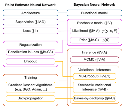
Figure 1: Illustration of the correspondence between the concepts used in deep learning for point-estimate neural networks and their counterparts in Bayesian neural networks (BNNs).

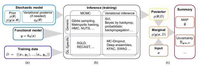
Figure 2: Workflow to design (a), train (b) and use a BNN for predictions (c).

Using Bayes’ formula to train a predictor can be understood as learning from the data $D$. In other words, the Bayesian paradigm not only offers a solid approach for the quantification of uncertainty in deep learning models but also provides a mathematical framework to understand many regularization techniques and learning strategies that are already used in classic deep learning [7] (Section IV-C3).

Bayesian neural networks (BNNs) [8, 9, 10] are stochastic neural networks trained using a Bayesian approach. There is a rich literature about BNNs and the related field of Bayesian deep learning, which is referred to by Wang and Yeung [11] as the conjoint use of deep learning for perception and traditional Bayesian models for inference. However, navigating through this literature is challenging without some prior background in Bayesian statistics. This brings an additional layer of complexity for deep learning practitioners interested in building and using BNNs.

This paper, conceived as a tutorial, presents a unified workflow to design, implement, train and evaluate a BNN (Figure 2). It also provides an overview of the relevant literature where a large number of approaches have been developed to efficiently train and use BNNs. A good knowledge of those different methods is a prerequisite for an efficient use of BNNs in big data applications of deep learning. In this tutorial, we assume that the reader is already familiar with the concepts of traditional deep learning such as artificial neural networks, training algorithms, supervision strategies, and loss functions [13]. This paper focuses on exploring the correspondences between traditional deep learning approaches and Bayesian methods (Figure 1). It is intended to motivate and help researchers and students to use BNNs in measuring uncertainty for problems in their respective fields of study and research, helping them relate their existing knowledge in deep learning to the relevant Bayesian methods.

The remaining parts of this paper are organized as follows. Section II introduces the concept of a BNN. Section III presents the motivations for BNNs as well as their applications. Section IV explains how to design the stochastic model associated with a BNN. Section V explores the most important algorithms used for Bayesian inference and how they were adapted for deep learning. Section VI reviews BNN simplification methods. Section VII presents the methods used to evaluate the performance of a BNN. Finally, Section VIII concludes the paper. The supplementary material contains a gallery of practical examples illustrating the theoretical concepts presented in Sections II, IV and V of the main paper. Each example source code is also available online on GitHub to provide implementation examples of the most important algorithms to work with BNNs.

II What is a Bayesian Neural Network?

A BNN is defined slightly differently across the literature, but a commonly agreed definition is that a BNN is a stochastic artificial neural network trained using Bayesian inference.

The goal of artificial neural networks (ANNs) is to represent an arbitrary function $\boldsymbol{y}=\Phi(\boldsymbol{x})$. Traditional ANNs such as feedforward networks and recurrent networks are built using one input layer $\boldsymbol{l}_{0}$, a succession of hidden layers $\boldsymbol{l}_{i},i=1,\dots,n-1$, and one output layer $\boldsymbol{l}_{n}$. (Here, $n+1$ is the total number of layers.) In the simplest architecture of feedforward networks, each layer $\boldsymbol{l}$ is represented as a linear transformation, followed by a nonlinear operation $s$, also known as an activation function:

$$\begin{array}[]{l}\boldsymbol{l}_{0}=\boldsymbol{x},\\ \boldsymbol{l}_{i}=s_{i}(\boldsymbol{W}_{i}\boldsymbol{l}_{i-1}~{}+~{}\boldsymbol{b}_{i})\quad\forall i\in[1,n],\\ \boldsymbol{y}=\boldsymbol{l}_{n}.\end{array}$$ (2)

Here, $\boldsymbol{\theta}=(\boldsymbol{W},\boldsymbol{b})$ are the parameters of the network, where $\boldsymbol{W}$ are the weights of the network connections and $\boldsymbol{b}$ the biases. A given ANN architecture represents a set of functions isomorphic to the set of possible parameters $\boldsymbol{\theta}$. Deep learning is the process of regressing the parameters $\boldsymbol{\theta}$ from the training data $D$, where $D$ is composed of a series of input $\boldsymbol{x}$ and their corresponding labels $\boldsymbol{y}$. The standard approach is to approximate a minimal cost point estimate of the network parameters $\hat{\boldsymbol{\theta}}$, i.e., a single value for each parameter (Figure 3(a)), using the backpropagation algorithm, with all other possible parametrizations of the network discarded. The cost function is often defined as the log likelihood of the training set, sometimes with a regularization term included. From a statistician’s point of view, this is a maximum likelihood estimation (MLE), or a maximum a posteriori (MAP) estimation when regularization is used.

The point estimate approach, which is the traditional approach in deep learning, is relatively easy to deploy with modern algorithms and software packages, but tends to lack explainability [14]. The final model might also generalize in unforeseen and overconfident ways on out-of-training-distribution data points [15, 16]. This property, in addition to the inability of ANNs to say “I don’t know”, is problematic for many critical applications. Of all the techniques that exist to mitigate this [17], stochastic neural networks have proven to be one of the most generic and flexible.

Stochastic neural networks are a type of ANN built by introducing stochastic components into the network. This is performed by giving the network either a stochastic activation (Figure 3(b)) or stochastic weights (Figure 3(c)) to simulate multiple possible models $\boldsymbol{\theta}$ with their associated probability distribution $p(\boldsymbol{\theta})$. Thus, BNNs can be considered a special case of ensemble learning [18].

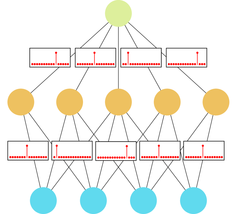
(a)

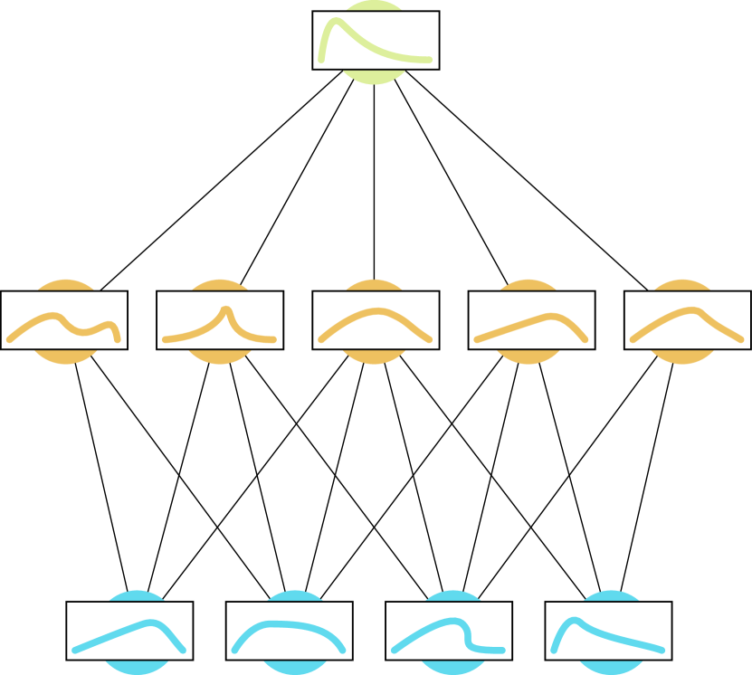
(b)

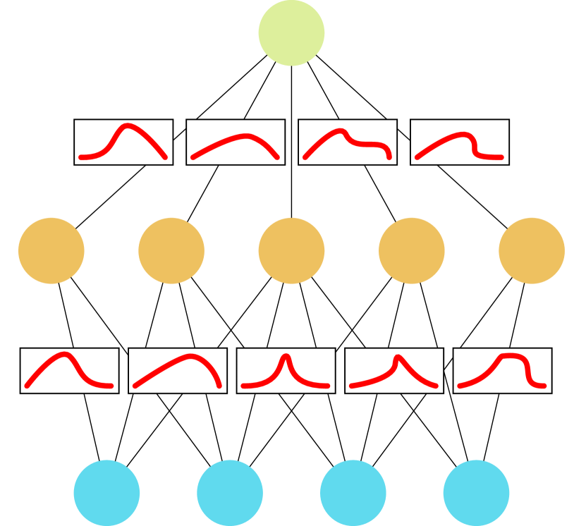
(c)

Figure 3: (3(a)) Point estimate neural network, (3(b)) stochastic neural network with a probability distribution for the activations, and (3(c)) stochastic neural network with a probability distribution over the weights.

The main motivation behind ensemble learning comes from the observation that aggregating the predictions of a large set of average-performing but independent predictors can lead to better predictions than a single well-performing expert predictor [19, 20]. Stochastic neural networks might improve their performance over their point estimate counterparts in a similar fashion, but this is not their main aim. Rather, the main goal of using a stochastic neural network architecture is to obtain a better idea of the uncertainty associated with the underlying processes. This is accomplished by comparing the predictions of multiple sampled model parametrizations $\boldsymbol{\theta}$. If the different models agree, then the uncertainty is low. If they disagree, then the uncertainty is high. This process can be summarized as follows:

$$\begin{array}[]{l}\boldsymbol{\theta}\sim p(\boldsymbol{\theta}),\\ \boldsymbol{y}=\Phi_{\boldsymbol{\theta}}(\boldsymbol{x})~{}+~{}\boldsymbol{\epsilon},\end{array}$$ (3)

where $\boldsymbol{\epsilon}$ represents random noise to account for the fact that the function $\Phi$ is only an approximation. A BNN can then be defined as any stochastic artificial neural network trained using Bayesian inference [21].

To design a BNN, the first step is the choice of a deep neural network architecture, i.e., a functional model. Then, one has to choose a stochastic model, i.e., a prior distribution over the possible model parametrization $p(\boldsymbol{\theta})$ and a prior confidence in the predictive power of the model $p(\boldsymbol{y}|\boldsymbol{x},\boldsymbol{\theta})$ (Figure 2a). The model parametrization can be considered to be the hypothesis $H$ and the training set is the data $D$. The choice of a BNN’s stochastic model is somehow equivalent to the choice of a loss function when training a point estimate neural network; see Section IV-C3. In the rest of this paper, we will denote the model parameters by $\boldsymbol{\theta}$, the training set by $D$, the training inputs by $D_{\boldsymbol{x}}$, and the training labels by $D_{\boldsymbol{y}}$. By applying Bayes’ theorem, and enforcing independence between the model parameters and the input, the Bayesian posterior can be written as:

$$\small p(\boldsymbol{\theta}|D)=\dfrac{p(D_{\boldsymbol{y}}|D_{\boldsymbol{x}},\boldsymbol{\theta})p(\boldsymbol{\theta})}{\int_{\boldsymbol{\theta}}p(D_{\boldsymbol{y}}|D_{\boldsymbol{x}},\boldsymbol{\theta^{\prime}})p(\boldsymbol{\theta^{\prime}})d\boldsymbol{\theta^{\prime}}}\propto p(D_{\boldsymbol{y}}|D_{\boldsymbol{x}},\boldsymbol{\theta})p(\boldsymbol{\theta}).$$ (4)

The Bayesian posterior for complex models such as artificial neural networks is a high dimensional and highly non-convex probability distribution [22]. This complexity makes computing and sampling it using standard methods an intractable problem, especially because computing the evidence $\int_{\boldsymbol{\theta}}p(D_{\boldsymbol{y}}|D_{\boldsymbol{x}},\boldsymbol{\theta^{\prime}})p(\boldsymbol{\theta^{\prime}})d\boldsymbol{\theta^{\prime}}$ is difficult. To address this problem, two broad approaches have been introduced: (1) Markov chain Monte Carlo and (2) variational inference. These are presented in more details in Section V.

When using a BNN for prediction, the probability distribution $p(\boldsymbol{y}|\boldsymbol{x},D)$ [12], called the marginal and which quantifies the model’s uncertainty on its prediction, is of particular interest. Given $p(\boldsymbol{\theta}|D)$, $p(\boldsymbol{y}|\boldsymbol{x},D)$ can be computed as:

$$p(\boldsymbol{y}|\boldsymbol{x},D)=\int_{\boldsymbol{\theta}}p(\boldsymbol{y}|\boldsymbol{x},\boldsymbol{\theta^{\prime}})p(\boldsymbol{\theta^{\prime}}|D)d\boldsymbol{\theta^{\prime}}.$$ (5)

In practice, $p(\boldsymbol{y}|\boldsymbol{x},D)$ is sampled indirectly using Equation (3). The final prediction can be summarized by statistics computed using a Monte Carlo approach (Figure 2c). A large set of weights $\boldsymbol{\theta}_{i}$ is sampled from the posterior and used to compute a series of possible outputs $\boldsymbol{y}_{i}$, as shown in Algorithm 1, which corresponds to samples from the marginal.

  Define $p(\boldsymbol{\theta}|D)=\dfrac{p(D_{\boldsymbol{y}}|D_{\boldsymbol{x}},\boldsymbol{\theta})p(\boldsymbol{\theta})}{\int_{\boldsymbol{\theta}}p(D_{\boldsymbol{y}}|D_{\boldsymbol{x}},\boldsymbol{\theta^{\prime}})p(\boldsymbol{\theta^{\prime}})d\boldsymbol{\theta^{\prime}}}$;

  for $i=0$ to $N$ do

     Draw $\boldsymbol{\theta}_{i}\sim p(\boldsymbol{\theta}|D)$;

     $\boldsymbol{y}_{i}=\Phi_{\boldsymbol{\theta}_{i}}(\boldsymbol{x})$;

  end for

  return  $Y=\{\boldsymbol{y}_{i}|i\in[0,N)\},~{}\Theta=\{\boldsymbol{\theta}_{i}|i\in[0,N)\}$;

Algorithm 1 Inference procedure for a BNN.

In Algorithm 1, $Y$ is a set of samples from $p(\boldsymbol{y}|\boldsymbol{x},D)$ and $\Theta$ a collection of samples from $p(\boldsymbol{\theta}|D)$. Usually, aggregates are computed on those samples to summarize the uncertainty of the BNN and obtain an estimator for the output $\boldsymbol{y}$. This estimator is denoted by $\boldsymbol{\hat{y}}$.

When performing regression, the procedure that is usually used to summarize the predictions of a BNN is model averaging [23]:

$$\boldsymbol{\hat{y}}=\dfrac{1}{|\Theta|}\sum_{\boldsymbol{\theta}_{i}\in\Theta}\Phi_{\boldsymbol{\theta}_{i}}(\boldsymbol{x}).$$ (6)

This approach is so common in ensemble learning that it is sometimes called ensembling. To quantify uncertainty, the covariance matrix can be computed as follows:

$$\boldsymbol{\Sigma}_{\boldsymbol{y}|\boldsymbol{x},D}=\dfrac{1}{|\Theta|-1}\sum_{\boldsymbol{\theta}_{i}\in\Theta}\left(\Phi_{\boldsymbol{\theta}_{i}}(\boldsymbol{x})-\boldsymbol{\hat{y}}\right)\left(\Phi_{\boldsymbol{\theta}_{i}}(\boldsymbol{x})-\boldsymbol{\hat{y}}\right)^{\intercal}.$$ (7)

When performing classification, the average model prediction will give the relative probability of each class, which can be considered a measure of uncertainty:

$$\boldsymbol{\hat{p}}=\dfrac{1}{|\Theta|}\sum_{\boldsymbol{\theta}_{i}\in\Theta}\Phi_{\boldsymbol{\theta}_{i}}(\boldsymbol{x}).$$ (8)

The final prediction is taken as the most likely class:

$$\boldsymbol{\hat{y}}=\operatorname*{arg\,max}_{i}p_{i}\in\boldsymbol{\hat{p}}.$$ (9)

This definition considers BNNs as discriminative models, i.e., models that aim to reconstruct a target variable $\boldsymbol{y}$ given observations $\boldsymbol{x}$. This excludes generative models, although there are examples of generative ANNs based on the Bayesian formalism, e.g., Variational autoencoders [24]. Those are out of the scope of this tutorial.

III Advantages of Bayesian methods for deep learning

One of the major critiques of Bayesian methods is that they rely on prior knowledge. This is especially true in deep learning, as deriving any insight about plausible parametrization for a given model before training is very challenging. Thus, why use Bayesian methods for deep learning? Discriminative models implicitly represent the conditional probability $p(\boldsymbol{y}|\boldsymbol{x},\boldsymbol{\theta})$, and Bayes’ formula is an appropriate tool to invert conditional probabilities, even if one has little insight about $p(\boldsymbol{\theta})$ a priori. While there are strong theoretical principles and schema upon which this Bayes’ formula can be based [25], this section focuses on some practical benefits of using BNNs.

First, Bayesian methods provide a natural approach to quantify uncertainty in deep learning since BNNs have better calibration than classical neural networks [26, 27, 28], i.e., their uncertainty is more consistent with the observed errors. They are less often overconfident or underconfident.

Second, a BNN allows distinguishing between the epistemic uncertainty $p(\boldsymbol{\theta}|D)$ and the aleatoric uncertainty $p(\boldsymbol{y}|\boldsymbol{x},\boldsymbol{\theta})$ [29]. This makes BNNs very data-efficient since they can learn from a small dataset without overfitting [30]. At prediction time, out-of-training distribution points will have high epistemic uncertainty instead of blindly giving a wrong prediction.

Third, the no-free-lunch theorem for machine learning [31] can be interpreted as stating that any supervised learning algorithm includes some implicit prior. Bayesian methods, when used correctly, will at least make the prior explicit. Integrating prior knowledge into ANNs, which work as black boxes, is difficult but not impossible. In Bayesian deep learning, priors are often considered as soft constraints, analogous to regularization, or data transformations such as data augmentation in traditional deep learning; see Section IV-C. Most regularization methods used for point estimate neural networks can be understood from a Bayesian perspective as setting a prior; see Section IV-C3.

Finally, the Bayesian paradigm enables the analysis of learning methods. A number of those methods initially not presented as Bayesian can be implicitly understood as being approximate Bayesian, e.g., regularization (Section IV-C3) or ensembling (Section V-E2). In fact, most of the BNNs used in practice rely on methods that are approximately or implicitly Bayesian (Section V-E) since the exact algorithms are computationally too expensive. The Bayesian paradigm also provides a systematic framework to design new learning and regularization strategies, even for point estimate models.

BNNs have been used in many fields to quantify uncertainty, e.g., in computer vision [32], network traffic monitoring [33], aviation [34], civil engineering [35, 36], hydrology [37], astronomy [38], electronics [39], and medicine [40]. BNNs are useful in (1) active learning [41, 42] where an oracle (e.g., a human annotator, a crowd, an expensive algorithm) can label new points from an unlabeled dataset $U$. The model needs to determine which points should be submitted to the oracle to maximize its performance while minimizing the calls to the oracle. BNNs are also useful in (2) online learning [43], where the model is retrained multiple times as new data become available. For active learning, data points in the training set with high epistemic uncertainty are scheduled to be labeled with higher priority; see Algorithm 2. In contrast, in online learning, previous posteriors can be recycled as priors when new data become available to avoid the so-called problem of catastrophic forgetting [44]; see Algorithm 3.

  while $U\neq\varnothing$ and $\boldsymbol{\Sigma}_{\boldsymbol{y}|\boldsymbol{x}_{max},D}<\text{threshold}$ and $C<\text{MaxC}$ do

     Draw $\Theta=\{\boldsymbol{\theta}_{i}\sim p(\boldsymbol{\theta}|D)|i\in[0,N)\}$;

     for $\boldsymbol{x}\in U$ do

        $\boldsymbol{\Sigma}_{\boldsymbol{y}|\boldsymbol{x},D}=\dfrac{1}{|\Theta|-1}\sum_{\boldsymbol{\theta}_{i}\in\Theta}\left(\Phi_{\boldsymbol{\theta}_{i}}(\boldsymbol{x})-\boldsymbol{\hat{y}}\right)\left(\Phi_{\boldsymbol{\theta}_{i}}(\boldsymbol{x})-\boldsymbol{\hat{y}}\right)^{\intercal}$;

        if $\boldsymbol{\Sigma}_{\boldsymbol{y}|\boldsymbol{x},D}>\boldsymbol{\Sigma}_{\boldsymbol{y}|\boldsymbol{x}_{max},D}$ then

           $\boldsymbol{x}_{max}=\boldsymbol{x}$;

        end if

     end for

     $D_{\boldsymbol{x}}=D_{\boldsymbol{x}}\cup\{\boldsymbol{x}_{\text{max}}\}$;

     $D_{\boldsymbol{y}}=D_{\boldsymbol{y}}\cup\{\text{Oracle}(\boldsymbol{x}_{\text{max}})\}$;

     $U=U\setminus\{\boldsymbol{x}_{\text{max}}\}$;

     $C=C+1$;

  end while

Algorithm 2 Active learning loop with a BNN.

  Define $p(\boldsymbol{\theta})=p(\boldsymbol{\theta})_{0}$;

  while true do

     Define $p(\boldsymbol{\theta}|D_{i})=\dfrac{p(D_{\boldsymbol{y},i}|D_{\boldsymbol{x},i},\boldsymbol{\theta})p(\boldsymbol{\theta})_{i}}{\int_{\boldsymbol{\theta}}.p(D_{\boldsymbol{y},i}|D_{\boldsymbol{x},i},\boldsymbol{\theta^{\prime}})p(\boldsymbol{\theta^{\prime}})_{i}d\boldsymbol{\theta^{\prime}}}$;

     Define $p(\boldsymbol{\theta})_{i+1}=p(\boldsymbol{\theta}|D_{i})$;

  end while

Algorithm 3 Online learning loop with a BNN.

IV Setting the stochastic model for a Bayesian Neural Network

Designing a BNN requires choosing a functional model and a stochastic model. This tutorial will not cover the design of the functional model, as almost any model used for point estimate networks can be used as a functional model for a BNN. Furthermore, a rich literature on the subject exists already; see, for example, [45]. Instead, this section will focus on how to design the stochastic model. Section IV-A introduces probabilistic graphical models (PGMs), a tool used to represent the relationships between the model’s stochastic variables. Section IV-B details how to derive the posterior for a BNN from its PGM. Section IV-C discusses how to choose the probability laws used as priors. Finally, Section IV-D presents how the choice of a PGM can affect the degree of supervision or incorporate other forms of prior knowledge into the model.

IV-A Probabilistic graphical models

(a)

(b)

(c)

(d)

(e)

Figure 4: The different symbols PGM, (4(a)) observed variables are in colored circles, (4(b)) unobserved variables are in white circles, (4(c)) deterministic variables are in dashed circles and (4(d)) parameters are in rectangles. Plates, represented as a rectangle around a subgraph, indicate multiple independent instances of the subgraph for a batch of variables $B$ (4(e)).

Probabilistic graphical models (PGMs) use graphs to represent the interdependence of multivariate stochastic variables and subsequently decompose their probability distributions. PGMs cover a large variety of models. The type of PGMs this tutorial focuses on are Bayesian belief networks (BBN), which are PGMs whose graphs are acyclic and directed. We refer the reader to [46] for more details on how to represent learning algorithms using general PGMs.

In a PGM, variables $\boldsymbol{v}_{i}$ are the nodes in the graph. Different symbols are used to distinguish the nature of the considered variables (Figure 4). A directed link, which is the only type of link allowed in a BBN, means that the probability distribution of the target variable is defined conditioned on the source variable. The fact that the BBN is acyclic allows the computation of the joint probability distribution of all the variables $\boldsymbol{v}_{i}$ in the graph:

$$p(\boldsymbol{v}_{1},...,\boldsymbol{v}_{n})=\prod_{i=1}^{n}p(\boldsymbol{v}_{i}|\text{parents}(\boldsymbol{v}_{i})).$$ (10)

The type of distribution used to define the conditional probabilities $p(\boldsymbol{v}_{i}|\text{parents}(\boldsymbol{v}_{i}))$ depends on the context. Once the conditional probabilities are defined, the BBN describes a data generation process. Parents are sampled before their children. This is always possible since the graph is acyclic. All the variables together represent a sample from the joint probability distribution $p(\boldsymbol{v}_{1},\dots,\boldsymbol{v}_{n})$.

Models usually learn from multiple examples sampled from the same distribution. To highlight this fact, the plate notation (Figure 4(e)) has been introduced. A plate indicates that the variables $(\boldsymbol{v}_{1},...,\boldsymbol{v}_{n})$ in the subgraph encapsulated by the plate are copied along a given batch dimension. A plate implies independence between all the duplicated nodes. This fact can be exploited to compute the joint probability of a batch $B=\left\{(\boldsymbol{v}_{1},...,\boldsymbol{v}_{n})_{b}:b=1,\dots,|B|\right\}$ as:

$$p(B)=\prod_{(\boldsymbol{v}_{1},\dots,\boldsymbol{v}_{n})\in B}p(\boldsymbol{v}_{1},\dots,\boldsymbol{v}_{n}).$$ (11)

In a PGM, the observed variables, depicted in Figure 4(a) using colored circles, are treated as the data. The unobserved, also called latent variables, represented by a white circle in Figure 4(b), are treated as the hypothesis. From the joint probability derived from the PGM, defining the posterior for the latent variables given the observed variables is straightforward using Bayes’ formula:

$$p(\boldsymbol{v}_{\text{latent}}|\boldsymbol{v}_{\text{obs}})\propto p(\boldsymbol{v}_{\text{obs}},\boldsymbol{v}_{\text{latent}}).$$ (12)

The joint distribution $p(\boldsymbol{v}_{\text{obs}},\boldsymbol{v}_{\text{latent}})$ is then used by the different inference algorithms; see Section V.

IV-B Defining the stochastic model of a BNN from a PGM

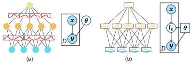
Figure 5: BBNs with (a) coefficients as stochastic variables and (b) activations as stochastic variables.

Consider the two models presented in Figure 5, with both the BNN and the corresponding BBN depicted. The BNN with stochastic weights (Figure 5a), if meant to perform regression, could represent the following data generation process:

$$\begin{array}[]{l}\boldsymbol{\theta}\sim p(\boldsymbol{\theta})=\mathcal{N}(\boldsymbol{\mu},\boldsymbol{\Sigma}),\\ \boldsymbol{y}\sim p(\boldsymbol{y}|\boldsymbol{x},\boldsymbol{\theta})=\mathcal{N}(\Phi_{\boldsymbol{\theta}}(\boldsymbol{x}),\boldsymbol{\Sigma}).\end{array}$$ (13)

The choice of using normal laws $\mathcal{N}(\boldsymbol{\mu},\boldsymbol{\Sigma})$, with mean $\boldsymbol{\mu}$ and covariance $\boldsymbol{\Sigma})$, is arbitrary but is common in practice because of its good mathematical properties.

For classification, the model samples the prediction from a categorical law $\text{Cat}(p_{i})$, i.e.,

$$\begin{array}[]{l}\boldsymbol{\theta}\sim p(\boldsymbol{\theta})=\mathcal{N}(\boldsymbol{\mu},\boldsymbol{\Sigma}),\\ \boldsymbol{y}\sim p(\boldsymbol{y}|\boldsymbol{x},\boldsymbol{\theta})=\text{Cat}(\Phi_{\boldsymbol{\theta}}(\boldsymbol{x})).\end{array}$$ (14)

Then, one can use the fact that multiple data points from the training set are independent, as indicated by the plate notation in Figure 5, to write the probability of the training set as:

$$p(D_{\boldsymbol{y}}|D_{\boldsymbol{x}},\boldsymbol{\theta})=\prod_{(\boldsymbol{x},\boldsymbol{y})\in D}p(\boldsymbol{y}|\boldsymbol{x},\boldsymbol{\theta}).$$ (15)

In the case of stochastic activations (Figure 5b), the data generation process might become:

$$\begin{array}[]{l}\boldsymbol{l}_{0}=\boldsymbol{x},\\ \boldsymbol{l}_{i}\sim p(\boldsymbol{l}_{i}|\boldsymbol{l}_{i-1})=s_{i}(\mathcal{N}(\boldsymbol{W}_{i}\boldsymbol{l}_{i-1}~{}+~{}\boldsymbol{b}_{i},\Sigma))\quad\forall i\in[1,n],\\ \boldsymbol{y}=\boldsymbol{l}_{n}.\end{array}$$ (16)

The formulation of the joint probability is slightly more complex as we have to account for the chain of dependencies spanned by the BBN over the multiple latent variables $\boldsymbol{l}_{[1,n-1]}$:

$$p(D_{\boldsymbol{y}},\boldsymbol{l}_{[1,n-1]}|D_{\boldsymbol{x}})=\prod_{(\boldsymbol{l}_{0},\boldsymbol{l}_{n})\in D}\left(\prod_{i=1}^{n}p(\boldsymbol{l}_{i}|\boldsymbol{l}_{i-1})\right).$$ (17)

It is sometimes possible, and often desirable, to define $p(\boldsymbol{l}_{i}|\boldsymbol{l}_{i-1})$ such that the BNNs described in Figure 5a and in Figure 5b can be considered equivalent. For instance, sampling $l$ as:

$$\begin{array}[]{l}\boldsymbol{W}\sim\mathcal{N}(\boldsymbol{\mu}_{\boldsymbol{W}},\boldsymbol{\Sigma}_{\boldsymbol{W}}),\\ \boldsymbol{b}\sim\mathcal{N}(\boldsymbol{\mu}_{\boldsymbol{b}},\boldsymbol{\Sigma}_{\boldsymbol{b}}),\\ \boldsymbol{l}=s(\boldsymbol{W}\boldsymbol{l}_{-1}+\boldsymbol{b})\end{array}$$ (18)

is equivalent to sampling $l$ as:

$$\boldsymbol{l}\sim s(\mathcal{N}(\boldsymbol{\mu}_{\boldsymbol{W}}\boldsymbol{l}_{-1}+\boldsymbol{\mu}_{\boldsymbol{b}},(\boldsymbol{I}\otimes\boldsymbol{l}_{-1})^{\intercal}\boldsymbol{\Sigma}_{\boldsymbol{W}}(\boldsymbol{I}\otimes\boldsymbol{l}_{-1})+\boldsymbol{\Sigma}_{\boldsymbol{b}})),$$ (19)

where $\otimes$ denotes a Kronecker product.

The basic Bayesian regression architecture shown in Figure 5a is more common in practice. The alternative architecture shown in Figure 5b is sometimes used as it allows compressing the number of variational parameters when using variational inference [47]; see also Section V.

IV-C Setting the priors

Setting the prior of a deep neural network is often not an intuitive task. The main problem is that it is not truly explicit how models with a very large number of parameters and a nontrivial architecture such as an ANN will generalize for a given parametrization [48]. In this Section, we first present the common practice, discuss the issues related to the statistical unidentifiability of ANNs, and then show the link between the prior for BNNs and regularization for the point estimate algorithms. Finally, we present a method to build the prior from high level knowledge.

IV-C1 A good default prior

For basic architectures such as Bayesian regression (Figure 5a), a standard procedure is to use a normal prior with a zero mean $\boldsymbol{0}$ and a diagonal covariance $\sigma\boldsymbol{I}$ on the coefficients of the network:

$$p(\boldsymbol{\theta})=\mathcal{N}(\boldsymbol{0},\sigma\boldsymbol{I}).$$ (20)

This approach is equivalent to a weighted $\ell_{2}$ regularization (with weights $1/\sigma$) when training a point estimate network, as will be demonstrated in Section IV-C3. The documentation of the probabilistic programming language Stan [49] provides examples on how to choose $\sigma$ knowing the expected scale of the considered parameters [50].

Although such an approach is often used in practice, there is no theoretical argument that makes it better than any other formulation [51]. The normal law is preferred due to its mathematical properties and the simple formulation of its log, which is used in most of the learning algorithms.

IV-C2 Addressing unidentifiability in Bayesian neural networks

One of the main problems with Bayesian deep learning is that deep neural networks are overparametrized models, i.e., they have many equivalent parametrizations [52]. This is an example of statistical unidentifiability, which can lead to complex multimodal posteriors that are hard to sample and approximate when training a BNN [22]. There are two solutions to deal with this issue: (1) changing the functional model parametrization, or (2) constraining the support of the prior to remove unidentifiability.

The two most common classes of nonuniqueness in ANNs are weight-space symmetry and scaling symmetry [53]. Both are not a concern for point estimate neural networks but might be for BNNs. Weight-space symmetry implies that one can build an equivalent parametrization of an ANN with at least one hidden layer. This is achieved by permuting two rows in $(\boldsymbol{W}_{i},\boldsymbol{b}_{i})$, the weights and their corresponding bias $\boldsymbol{b}_{i}$, of one of the hidden layers as well as the corresponding columns in the following layer’s weight matrix $\boldsymbol{W}_{i+1}$. This means that as the number of hidden layers and the number of units in the hidden layers grow, the number of equivalent representations, which would roughly correspond to the modes in the posterior distribution, grows factorially. A mitigation strategy is to enforce the bias vector in each layer to be sorted in an ascending or a descending order. However, the practical effects of doing so may be to degrade optimization: weight-space symmetry may implicitly support the exploration of the parameter space during the early stages of the optimization.

Scaling symmetry is an unidentifiability problem arising when using nonlinearities with the property $s(\alpha x)=\alpha s(x)$, which is the case of RELU and Leaky-RELU, two popular nonlinearities in modern machine learning. In this case, assigning the weights $\boldsymbol{W}_{l},\boldsymbol{W}_{l+1}$ to two consecutive layers $l$ and $l+1$ becomes strictly equivalent to assigning $\alpha\boldsymbol{W}_{l},(1/\alpha)\boldsymbol{W}_{l+1}$. This can reduce the convergence speed for point estimate neural networks, a problem that is addressed in practice with various activation normalization techniques [54]. BNNs are slightly more complex as the scaling symmetry influences the posterior shape, making it harder to approximate. Givens transformations (also called Givens rotations) have been proposed as a mean to constrain the norm of the hidden layers [53] and address the scaling symmetry issue. In practice, using a Gaussian prior already reduces the scaling symmetry problem, as it favors weights with the same Frobenius norm on each layer. A soft version of the activation normalization can also be implemented by using a consistency condition; see Section IV-C4. The additional complexity associated with sampling the network parameters in a constrained space to perfectly remove the scaling symmetry is computationally prohibitive. We provide, in the Practical Example III of the Supplementary Material , additional discussion on this issue using the ”Paperfold” practical example.

(a) Noisy labels

(b) Semi-supervised learning

(c) Data augmentation

(d) Meta-learning

(e) Self-supervised learning

Figure 6: Different examples of PGMs to adapt the learning strategy for a given BNN (with stochastic weights).

IV-C3 The link between regularization and priors

The usual learning procedure for a point estimate neural network is to find the set of parameters $\boldsymbol{\theta}$ that minimize a loss function built using the training set $D$:

$$\boldsymbol{\hat{\theta}}=\operatorname*{arg\,min}_{\boldsymbol{\theta}}~{}\text{loss}_{D_{x},D_{y}}(\boldsymbol{\theta}).$$ (21)

Assuming that the loss is defined as minus the log-likelihood function up to an additive constant, the problem can be rewritten as:

$$\boldsymbol{\hat{\theta}}=\operatorname*{arg\,max}_{\boldsymbol{\theta}}~{}p(D_{\boldsymbol{y}}|D_{\boldsymbol{x}},\boldsymbol{\theta}),$$ (22)

which would be the first half of the model according to the Bayesian paradigm. Now, assume that we also have a prior for $\boldsymbol{\theta}$, and we want to find the most likely point estimate from the posterior. The problem can be reformulated as:

$$\boldsymbol{\hat{\theta}}=\operatorname*{arg\,max}_{\boldsymbol{\theta}}~{}p(D_{\boldsymbol{y}}|D_{\boldsymbol{x}},\boldsymbol{\theta})p(\boldsymbol{\theta}).$$ (23)

Next, one would go back to a log-likelihood formulation:

$$\boldsymbol{\hat{\theta}}=\operatorname*{arg\,min}_{\boldsymbol{\theta}}~{}\text{loss}_{D_{x},D_{y}}(\boldsymbol{\theta})+\text{reg}(\boldsymbol{\theta}),$$ (24)

which is easier to optimize. Equation (24) is how regularization is usually applied in machine learning and in many other fields. Another argument, less formal, is that regularization acts as a soft constraint on the search space, in a manner similar to what a prior does for a posterior.

IV-C4 Prior with a consistency condition

Regularization can also be implemented with a consistency condition $C(\boldsymbol{\theta},\boldsymbol{x})$, which is a function used to measure how well the model respects some hypothesis given a parametrization $\boldsymbol{\theta}$ and an input $\boldsymbol{x}$. For example, $C$ can be set to favor sparse or regular predictions to encourage monotonicity of predictions with respect to some input variables (e.g., the probability of getting the flu increases with age), or to favor decision boundaries in low density regions when using semi-supervised learning; see Section IV-D1. $C$ can be seen as the relative log likelihood of a prediction given the input $\boldsymbol{x}$ and parameter set $\boldsymbol{\theta}$. Thus, it can be included in the prior. To this end, $C$ should be averaged over all possible inputs:

$$C(\boldsymbol{\theta})=\int_{\boldsymbol{x}}C(\boldsymbol{\theta},\boldsymbol{x})p(\boldsymbol{x})d\boldsymbol{x}.$$ (25)

In practice, as $p(\boldsymbol{x})$ is unknown, $C(\boldsymbol{\theta})$ is approximated from the features in the training set:

$$C(\boldsymbol{\theta})\approx\dfrac{1}{|D_{\boldsymbol{x}}|}\sum_{\boldsymbol{x}\in|D_{\boldsymbol{x}}|}C(\boldsymbol{\theta},\boldsymbol{x}).$$ (26)

We can now write a function proportional to the prior with the consistency condition included:

$$p(\boldsymbol{\theta}|D_{\boldsymbol{x}})\propto p(\boldsymbol{\theta})\operatorname{exp}\left(-\dfrac{1}{|D_{\boldsymbol{x}}|}\sum_{\boldsymbol{x}\in|D_{\boldsymbol{x}}|}C(\boldsymbol{\theta},\boldsymbol{x})\right),$$ (27)

where $p(\boldsymbol{\theta})$ is the prior without the consistency condition.

IV-D Degree of supervision and alternative forms of prior knowledge

The architecture presented in Section IV-B focuses mainly on the use of BNNs in a supervised learning setting. However, in real world applications, obtaining ground-truth labels can be expensive. Thus, new learning strategies should be adopted [55]. We will now present how to adapt BNNs for different degrees of supervision. While doing so, we will also demonstrate how PGMs in general and BBNs in particular are useful in designing or interpreting learning strategies. In particular, the formulation of the Bayesian posterior, which is derived from the different PGMs presented in Figure 6, can also be used for a point estimate neural network to obtain a suitable loss function to search for an MAP estimator for the parameters (Section IV-C3). We also provide a practical example in the Supplementary Material (Practical Example II) to illustrate how such strategies can be implemented for an actual BNN.

IV-D1 Noisy labels and semi-supervised learning

The inputs $D_{\boldsymbol{x}}$ in the training sets can be uncertain, either because the labels $D_{\boldsymbol{y}}$ are corrupted by noise [56], or because labels are missing for a number of points. In the case of noisy labels, one should extend the BBN to add a new variable for the noisy labels $\boldsymbol{\tilde{y}}$ conditioned on $\boldsymbol{y}$ (Figure 6(a)). It is common, as the noise level itself is often unknown, to add a variable $\boldsymbol{\sigma}$ to characterize the noise. Frenay et al.  [57] proposed a taxonomy of the different approaches used to integrate $\boldsymbol{\sigma}$ in a PGM (Figure 7). They distinguish three cases: noise completely at random (NCAR); noise at random (NAR); and noise not at random (NNAR) models. In the NCAR model, the noise $\boldsymbol{\sigma}$ is independent of any other variable, i.e., it is homoscedastic. In the NAR model, $\boldsymbol{\sigma}$ is dependent on the true label $\boldsymbol{y}$ but remains independent of the features. NNAC models also account for the influence of the features $\boldsymbol{x}$, e.g., if the level of noise in an image increases, then the probability that the image has been mislabeled also increases. Both NAR and NNAC models represent heteroscedastic, i.e., the antonym of homoscedastic, noise.

(a)

(b)

(c)

Figure 7: BBNs corresponding to (7(a)) the noise completely at random (NCAR), (7(b)) noise at random (NAR) and (7(c)) noise not at random (NNAR) models from [57].

These noise-aware PGMs are slightly more complex than a purely supervised BNN, as presented in Section IV-B. However, they can be treated in a similar fashion by deriving the formula for the posterior from the PGM (Equation (12)) and applying the chosen inference algorithm. For the NNAR model, the most generic stochastic model of the three described above (since the NCAR and NAR models are special cases of the NNAR model), the posterior becomes:

$$\small p(\boldsymbol{y},\boldsymbol{\sigma},\boldsymbol{\theta}|D)~{}\propto~{}p(D_{\boldsymbol{\tilde{y}}}|\boldsymbol{y},\boldsymbol{\sigma})p(\boldsymbol{\sigma}|D_{\boldsymbol{x}},\boldsymbol{y})p(\boldsymbol{y}|D_{\boldsymbol{x}},\boldsymbol{\theta})p(\boldsymbol{\theta}).$$ (28)

During the prediction phase, $\boldsymbol{y}$ and $\boldsymbol{\sigma}$ can simply be discarded for each tuple $(\boldsymbol{y},\boldsymbol{\sigma},\boldsymbol{\theta})$ sampled from the posterior.

In the case of partially labeled data (Figure 6(b)), also known as semi-supervised learning, the dataset $D$ is split into labeled $L$ and unlabeled $U$ examples. In theory, this PGM can be considered equivalent to the one used in the supervised learning case depicted in Figure 5a, but in this case the unobserved data $U$ would bring no information. The additional information of unlabeled data comes from the prior and only the prior. Similar to traditional machine learning, the most common approaches to implement semi-supervised learning in Bayesian learning are either to use some type of data-driven regularization [58] or to rely on pseudo labels [59].

Data-driven regularization implies modifying the prior assumptions, and thus the stochastic model, to be able to extract meaningful information from the unlabeled dataset $U$. There are two common ways to approach this process. The first one is to condition the prior distribution of the model parameters on the unlabeled examples to favor certain properties of the model, such as a decision boundary in a low density region, using a distribution $p(\boldsymbol{\theta}|U)$ instead of $p(\boldsymbol{\theta})$. This implies formulating the stochastic model as:

$$p(\boldsymbol{\theta}|D)\propto p(L_{\boldsymbol{y}}|L_{\boldsymbol{x}},\boldsymbol{\theta})p(\boldsymbol{\theta}|U),$$ (29)

where $p(\boldsymbol{\theta}|U)$ is a prior with a consistency condition, as defined in Equation (27). The consistency condition usually expresses the fact that points that are close to each other should lead to the same prediction, e.g., graph Laplacian norm regularization [60].

The second way is to assume some kind of dependency across the observed and unobserved labels in the dataset. This type of semi-supervised Bayesian learning relies either on an undirected PGM [61] to build the prior or at least does not assume independence between different training pairs $(\boldsymbol{x},\boldsymbol{y})$ [62]. To keep things simple, we represent this fact by dropping the plate around $\boldsymbol{y}$ in Figure 6(b). The posterior is written in the usual way (Equation (4)). The main difference is that $p(D_{\boldsymbol{y}}|D_{\boldsymbol{x}},\boldsymbol{\theta})$ is chosen to enforce some kind of consistency across the dataset. For example, one can assume that two close points are likely to have similar labels $\boldsymbol{y}$ with a level of uncertainty that increases with the distance.

Both approaches have a similar effect and the choice of one over the other will depend on the mathematical formulation favored to build the model.

The semi-supervised learning strategy can also be reformulated as having a weak predictor capable of generating some pseudo labels $\boldsymbol{\tilde{y}}$, sometimes with some confidence level. Many of the algorithms used for semi-supervised learning use an initial version of the model trained with the labeled examples [63] to generate the pseudo labels $\boldsymbol{\tilde{y}}$ and train the final model with $\boldsymbol{\tilde{y}}$. This is problematic for BNNs. When the prediction uncertainty is accounted for, reducing the uncertainty associated with the unlabeled data becomes impossible, at least not without an additional hypothesis in the prior. Even if it is less current in practice, using a simpler model [64] to obtain the pseudo labels can help mitigate that problem.

IV-D2 Data augmentation

Data augmentation in machine learning is a strategy that is used to significantly increase the diversity of the data $D$ available to train deep models, without actually collecting new data. It relies on transformations that act on the input but have no or very low probability to change the label (or at least do so in a predictable way) to generate an augmented dataset $A(D)$. Examples of such transformations include applying rotations, flipping or adding noise in the case of images. Data augmentation is now at the forefront of state-of-the-art techniques in computer vision [59] and increasingly in natural language processing [65].

The augmented dataset $A(D)$ could contain an infinite set of possible variants of the initial dataset $D$, e.g., when using continuous transforms such as rotations or additional noise. To achieve this in practice, $A(D)$ is sampled on the fly during training, rather than generating in advance all possible augmentations in the training set. This process is straightforward when training point estimate neural networks, but there are some subtleties when applying it in Bayesian statistics. The main concern is that the posterior of interest is $p(\boldsymbol{\phi}|D,Aug)$, where $Aug$ represents some knowledge about augmentation, not $p(\boldsymbol{\phi}|A(D),D)$, since $A(D)$ is not observed. From a Bayesian perspective, the additional information is brought by the knowledge of the augmentation process rather than by some additional data. Stated otherwise, the data augmentation is a part of the stochastic model (Figure 6(c)).

The idea is that if one is given data $D$, then one could also have been given data $D^{\prime}$, where each element in $D$ is replaced by an augmentation. Then, $D^{\prime}$ is a different perspective of the data $D$. To model this, we have the augmentation distribution $p(\boldsymbol{x}^{\prime}|\boldsymbol{x},Aug)$ that augments the observed data using the augmentation model $Aug$ to generate (probabilistically) $x^{\prime}$, which represents data in the vicinity of $x$ (Figure 6(c)). $x^{\prime}$ can then be marginalized to simplify the stochastic model. The posterior is given by:

$$\small p(\boldsymbol{\theta}|\boldsymbol{x},\boldsymbol{y},Aug)\propto\left(\int_{\boldsymbol{x}^{\prime}}p(\boldsymbol{y}|\boldsymbol{x}^{\prime},\boldsymbol{\theta})p(\boldsymbol{x}^{\prime}|\boldsymbol{x},Aug)d\boldsymbol{x}^{\prime}\right)p(\boldsymbol{\theta}).$$ (30)

This is a probabilistic counterpart to vicinal risk [66].

The integral in Equation (30) can be approximated using Monte Carlo integration by sampling a small set of augmentations $A_{x}$ according to $p(x^{\prime}|x,Aug)$ and averaging:

$$p(y|x,\boldsymbol{\theta},Aug)\approx\dfrac{1}{|A_{x}|}\sum_{x^{\prime}\in A_{x}}p(y|x^{\prime},\boldsymbol{\theta}).$$ (31)

When training using a Monte-Carlo-based estimate of the loss, $A_{x}$ can contain as few as a single element as long as it is resampled for each optimization iteration. This greatly simplifies the evaluation of Equation (31).

An extension of this approach works in the context of semi-supervised learning. The prior can be designed to encourage consistency of predictions under augmentation [67, 59], using unlabeled data to build the samples for the consistency condition, as defined in Equation (27). Note that this does not add labeling to the unlabeled examples but only adds a term to encourage consistency between the labels for an unlabeled data point and its augmentation.

IV-D3 Meta-learning, transfer learning, and self-supervised learning

Meta-learning [68], in the broadest sense, is the use of machine learning algorithms to assist in the training and optimization of other machine learning models. The meta knowledge acquired by meta-learning can be distinguished from standard knowledge in the sense that it is applicable to a set of related tasks rather than a single task.

Transfer learning designates methods that reuse some intermediate knowledge acquired on a given problem to address a different problem. In deep learning, it is used mostly for domain adaptation, when labeled data are abundant in a domain that is in some way similar to the domain of interest but scarce in the domain of interest [69]. Alternatively, pre-trained models [70] could be used to study large architectures whose complete training would be very computationally expensive.

Self-supervised learning is a learning strategy where the data themselves provide the labels [71]. Since the labels directly obtainable from the data do not match the task of interest, the problem is approached by learning a pretext (or proxy) task in addition to the task of interest. The use of self-supervision is now generally regarded as an essential step in some areas. For instance, in natural language processing, most state-of-the-art methods use these pre-trained models [70]. In addition, modern deep learning-based 3D object reconstruction [72] and disparity estimation in stereo vision [73] rely on self-supervised learning to overcome the time-consuming manual annotation of training data.

A common approach for meta-learning in Bayesian statistics is to recast the problem as hierarchical Bayes [74], with the prior $p(\boldsymbol{\theta}_{t}|\boldsymbol{\xi})$ for each task conditioned on a new global variable $\boldsymbol{\xi}$ (Figure 6(d)). $\boldsymbol{\xi}$ can represent continuous metaparameters or discrete information about the structure of the BNN, i.e., to learn probable functional models, or the underlying subgraph of the PGM, i.e., to learn probable stochastic models. Multiple levels can be added to organize the tasks in a more complex hierarchy if needed. Here, we present only the case with one level since the generalization is straightforward. With this broad Bayesian understanding of meta-learning, both transfer learning and self-supervised learning are special cases of meta-learning. The general posterior becomes:

$$p(\boldsymbol{\theta},\boldsymbol{\xi}|D)\propto\left(\prod_{t\in T}p(D^{t}_{\boldsymbol{y}}|D^{t}_{\boldsymbol{x}},\boldsymbol{\theta}_{t})p(\boldsymbol{\theta}_{t}|\boldsymbol{\xi})\right)p(\boldsymbol{\xi}).$$ (32)

In practice, the problem is often approached with empirical Bayes (Section V-D), and only a point estimate $\boldsymbol{\hat{\xi}}$ is considered for the global variable, ideally the MAP estimate obtained by marginalizing $p(\boldsymbol{\theta},\boldsymbol{\xi}|D)$ and selecting the most likely point, but this is not always the case.

In transfer learning, the usual approach would be to set $\boldsymbol{\hat{\xi}}=\boldsymbol{\theta}_{m}$, with $\boldsymbol{\theta}_{m}$ being the coefficients of the main task. The new prior can then be obtained from $\boldsymbol{\hat{\xi}}$, for example:

$$p(\boldsymbol{\theta}|\boldsymbol{\xi})=\mathcal{N}((\tau(\boldsymbol{\xi}),\boldsymbol{0}),\sigma\boldsymbol{I}),$$ (33)

where $\tau$ is a selection of the parameters to transfer and $\sigma$ is a parameter to tune manually. Unselected parameters are assigned a new prior, with a mean of $0$ by convention. If a BNN has been trained for the main task, then $\sigma$ can be estimated from the previous posterior, with an increment to account for the additional uncertainty caused by the domain shift.

Self-supervised learning can be implemented in two steps. The first step learns the pretext task while the second one performs transfer learning. This can be considered overly complex but might be required if the pretext task has a high computational complexity (e.g., BERT models in natural language processing [70]). Recent contributions [75] have shown that jointly learning the pretext task and the final task (Figure 6(e)) can improve the results obtained in self-supervised learning. This approach, which is closer to hierarchical Bayes, also allows setting the prior a single time while still retaining the benefits of self-supervised learning.

V Bayesian Inference algorithms

A priori, a BNN does not require a learning phase as one just needs to sample the posterior and do model averaging; see Algorithm 1. However, sampling the posterior is not easy in the general case. While the conditional probability $P(D|H)$ of the data and the probability $P(H)$ of the model are given by the stochastic model, the integral for the evidence term $\int_{H}P(D|H^{\prime})P(H^{\prime})dH^{\prime}$ might be excessively difficult to compute. For nontrivial models, even if the evidence has been computed, directly sampling the posterior is prohibitively difficult due to the high dimensionality of the sampling space. Instead of using traditional methods, e.g., inversion sampling or rejection sampling to sample the posterior, dedicated algorithms are used. The most popular ones are Markov chain Monte Carlo (MCMC) methods [76], a family of algorithms that exactly sample the posterior, or variational inference [77], a method for learning an approximation of the posterior; see Figure 2.

This section reviews these methods. First, in subsection V-A and V-B, we introduce MCMC and variational inference as they are used in traditional Bayesian statistics. Then, in subsection V-E, we review different simplifications or approximations that have been proposed for deep learning. We also provide a practical example in the Supplementary Material (Practical example III), which compares different learning strategies.

V-A Markov Chain Monte Carlo (MCMC)

The idea behind MCMC methods is to construct a Markov chain, a sequence of random samples $S_{i}$, which probabilistically depend only on the previous sample $S_{i-1}$, such that the $S_{i}$ are distributed following a desired distribution. Unlike standard sampling methods such as rejection or inversion sampling, most MCMC algorithms require an initial burn-in time before the Markov chain converges to the desired distribution. Moreover, the successive $S_{i}$’s might be autocorrelated. This means that a large set of samples $\Theta$ has to be generated and subsampled to obtain approximately independent samples from the underlying distribution. The final collection of samples $\Theta$ has to be stored after training, which is expensive for most deep learning models.

Despite their inherent drawbacks, MCMC methods can be considered among the best available and the most popular solutions for sampling from exact posterior distributions in Bayesian statistics [78]. However, not all MCMC algorithms are relevant for Bayesian deep learning. Gibbs sampling [79], for example, is very popular in general statistics and unsupervised machine learning but is very ill-suited for BNNs. The most relevant MCMC method for BNNs is the Metropolis-Hastings algorithm [80]. The property that makes the Metropolis-Hasting algorithm popular is that it does not require knowledge about the exact probability distribution $P(\boldsymbol{x})$ to sample from. Instead, a function $f(\boldsymbol{x})$ that is proportional to that distribution is sufficient. This is the case of a Bayesian posterior distribution, which is usually quite easy to compute except for the evidence term.

The Metropolis-Hasting algorithm, see Algorithm 4, starts with a random initial guess, $\boldsymbol{\theta}_{0}$, and then samples a new candidate point $\theta^{\prime}$ around the previous $\theta$, using a proposal distribution $Q(\theta^{\prime}|\theta)$. If $\theta^{\prime}$ is more likely than $\theta$ according to the target distribution, it is accepted. If it is less likely, it is accepted with a certain probability or rejected otherwise.

  Draw $\boldsymbol{\theta}_{0}\sim Initial~{}probability~{}distribution$;

  while $n=0$ to $N$ do

     Draw $\boldsymbol{\theta}^{\prime}\sim Q(\boldsymbol{\theta}^{\prime}|\boldsymbol{\theta}_{n})$;

     $p=\min\left(1,\dfrac{Q(\boldsymbol{\theta}^{\prime}|\boldsymbol{\theta}_{n})}{Q(\boldsymbol{\theta}_{n}|\boldsymbol{\theta}^{\prime})}\dfrac{f(\boldsymbol{\theta}^{\prime})}{f(\boldsymbol{\theta}_{n})}\right)$;

     Draw $k\sim\text{Bernoulli}(p)$;

     if $k$ then

        $\boldsymbol{\theta}_{n+1}=\boldsymbol{\theta}^{\prime}$;

        $n=n+1$;

     end if

  end while

Algorithm 4 Metropolis-Hasting algorithm.

The acceptance probability $p$ can be simplified if $Q$ is chosen to be symmetric, i.e., $Q(\boldsymbol{\theta}^{\prime}|\boldsymbol{\theta}_{n})=Q(\boldsymbol{\theta}_{n}|\boldsymbol{\theta}^{\prime})$. The formula for the acceptance rate then becomes:

$$p=\min\left(1,\dfrac{f(\boldsymbol{\theta}^{\prime})}{f(\boldsymbol{\theta}_{n})}\right).$$ (34)

In this situation, the algorithm is simply called the Metropolis method. Common choices for $Q$ can be a normal distribution $Q(\boldsymbol{\theta}^{\prime}|\boldsymbol{\theta}_{n})=\mathcal{N}(\boldsymbol{\theta}_{n},\sigma^{2})$, or a uniform distribution $Q(\boldsymbol{\theta}^{\prime}|\boldsymbol{\theta}_{n})=\mathcal{U}(\boldsymbol{\theta}_{n}-\boldsymbol{\varepsilon},\boldsymbol{\theta}_{n}+\boldsymbol{\varepsilon})$, centered around the previous sample. To deal with non-symmetric proposal distributions, e.g., to accommodate a constraint in the model such as a bounded domain, one has to take into account the correction term imposed by the full Metropolis-Hasting algorithm.

The spread of $Q(\boldsymbol{\theta}^{\prime}|\boldsymbol{\theta}_{n})$ has to be tweaked. If it is too large, the rejection rate will be too high. If it is too small, the samples will be more autocorrelated. There is no general method to tweak those parameters. However, a clever strategy to obtain the new proposed sample $\boldsymbol{\theta}^{\prime}$ can reduce their impact. This is why the Hamiltonian Monte-Carlo method has been proposed.

The Hamiltonian Monte Carlo algorithm (HMC) [81] is another example of Metropolis-Hasting algorithms for continuous distributions. It is designed with a clever scheme to draw a new proposal $\boldsymbol{\theta}^{\prime}$ to ensure that as few samples as possible are rejected and there is as few correlation as possible between samples. In addition, the HMC’s burn-in time is extremely short compared to the standard Metropolis-Hasting algorithm.

Most software packages for Bayesian statistics implement the No-U-Turn sampler (NUTS for short) [82], which is an improvement over the classic HMC algorithm allowing the hyperparameters of the algorithm to be automatically tweaked instead of manually setting them.

V-B Variational inference

MCMC algorithms are the best tools for sampling from the exact posterior. However, their lack of scalability has made them less popular for BNNs, given the size of the models under consideration. Variational inference [77], which scales better than MCMC algorithms, gained considerable popularity. Variational inference is not an exact method. Rather than allowing sampling from the exact posterior, the idea is to have a distribution $q_{\phi}(H)$, called the variational distribution, parametrized by a set of parameters $\boldsymbol{\phi}$. The values of the parameters $\boldsymbol{\phi}$ are then learned such that the variational distribution $q_{\phi}(H)$ is as close as possible to the exact posterior $P(H|D)$. The measure of closeness that is commonly used is the Kullback-Leibler divergence (KL-divergence) [83]. It measures the differences between probability distributions based on Shannon’s information theory [84]. The KL-divergence represents the average number of additional bits required to encode a sample from $P$ using a code optimized for $q$. For Bayesian inference, it is computed as:

$$D_{KL}(q_{\phi}||P)=\int_{H}q_{\phi}(H^{\prime})\log\left(\dfrac{q_{\phi}(H^{\prime})}{P(H^{\prime}|D)}\right)dH^{\prime}.$$ (35)

There is an apparent problem here, which is, to compute $D_{KL}(q_{\phi}||P)$, one needs to compute $P(H|D)$ anyway. To overcome this, a different, easily derived formula called the evidence lower bound, or ELBO, serves as a loss:

$$\small\int_{H}q_{\phi}(H^{\prime})\log\left(\dfrac{P(H^{\prime},D)}{q_{\phi}(H^{\prime})}\right)dH^{\prime}=\log(P(D))-D_{KL}(q_{\phi}||P).$$ (36)

Since $\log(P(D))$ only depends on the prior, minimizing $D_{KL}(q_{\phi}||P)$ is equivalent to maximizing the ELBO.

The most popular method to optimize the ELBO is stochastic variational inference (SVI) [85], which is in fact the stochastic gradient descent method applied to variational inference. This allows the algorithm to scale to the large datasets that are encountered in modern machine learning, since the ELBO can be computed on a single mini-batch at each iteration.

Convergence, when learning the posterior with SVI, will be slow compared to the usual gradient descent. Moreover, most implementations use a small number of samples to evaluate the ELBO, often just one, before taking a gradient step. In other words, the ELBO estimate will be noisy at each iteration.

In traditional machine learning and statistics, $q_{\phi}(H)$ is mostly constructed from distributions in the exponential family, e.g., multivariate normal [86], Gamma and Dirichlet distributions. The ELBO can then be dramatically simplified into components [87] leading to a generalization of the well-known expectation-maximization algorithm. To account for correlations between the large number of parameters, certain approximations are made. For instance, block diagonal [88] or low rank plus diagonal [89] covariance matrices can be used to reduce the number of variational parameters $\boldsymbol{\phi}$ from $\mathcal{O}(n^{2})$ to $\mathcal{O}(n)$, where $n$ is the number of model parameters $\boldsymbol{\theta}$. Appendix A gives more details on how these simplifications are implemented in practice.

V-C Bayes by backpropagation

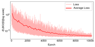
Figure 8: Typical training curve for Bayes-by-backprop.

Variational inference offers a good mathematical tool for Bayesian inference, but it needs to be adapted to deep learning. The main problem is that stochasticity stops backpropagation from functioning at the internal nodes of a network [46]. Different solutions have been proposed to mitigate this problem, including probabilistic backpropagation [90] or Bayes-by-backprop [91]. The latter may appear more familiar to deep learning practitioners. We will thus focus on Bayes-by-backprop in this tutorial. Bayes-by-backprop is indeed a practical implementation of SVI combined with a reparametrization trick [92] to ensure backpropagation works as usual.

The idea is to use a random variable $\varepsilon\sim q(\varepsilon)$ as a nonvariational source of noise. $\boldsymbol{\theta}$ is not sampled directly but obtained via a deterministic transformation $t(\varepsilon,\boldsymbol{\phi})$ such that $\boldsymbol{\theta}=t(\varepsilon,\boldsymbol{\phi})$ follows $q_{\phi}(\boldsymbol{\theta})$. $\varepsilon$ is sampled and thus changes at each iteration but can still be considered a constant with regard to other variables. All other transformations being non-stochastic, backpropagation works as usual for the variational parameters $\boldsymbol{\phi}$, meaning the training loop can be implemented analogous to the training loop of a non-stochastic neural network; see Algorithm 5. The general formula for the ELBO becomes:

$$\small\int_{\varepsilon}q_{\phi}(t(\varepsilon,\boldsymbol{\phi}))\log\left(\dfrac{P(t(\varepsilon,\boldsymbol{\phi}),D)}{q_{\phi}(t(\varepsilon,\boldsymbol{\phi}))}\right)\left|\text{Det}(\nabla_{\varepsilon}t(\varepsilon,\boldsymbol{\phi}))\right|d\varepsilon.$$ (37)

This is tedious to work with. Instead, to estimate the gradient of the ELBO, Blundell et al. [91] proposed to use the fact that if $q_{\phi}(\boldsymbol{\theta})d\boldsymbol{\theta}=q(\varepsilon)d\varepsilon$, then for a differentiable function $f(\boldsymbol{\theta},\boldsymbol{\phi})$, we have:

$$\footnotesize\dfrac{\partial}{\partial\boldsymbol{\phi}}\int_{\boldsymbol{\phi}}q_{\phi}(\boldsymbol{\theta}^{\prime})f(\boldsymbol{\theta}^{\prime},\boldsymbol{\phi})d\boldsymbol{\theta}^{\prime}=\int_{\varepsilon}q(\varepsilon)\left(\dfrac{\partial f(\boldsymbol{\theta},\boldsymbol{\phi})}{\partial\boldsymbol{\theta}}\dfrac{\partial\boldsymbol{\theta}}{\partial\boldsymbol{\phi}}+\dfrac{\partial f(\boldsymbol{\theta},\boldsymbol{\phi})}{\partial\boldsymbol{\phi}}\right)d\varepsilon.$$ (38)

A proof is provided in [91]. We also provide in Appendix B an alternative proof to give more details on when we can assume $q_{\phi}(\boldsymbol{\theta})d\boldsymbol{\theta}=q(\varepsilon)d\varepsilon$. A sufficient condition is for $t(\varepsilon,\boldsymbol{\phi})$ to be invertible with respect to $\varepsilon$ and the distributions $q(\varepsilon)$ and $q_{\phi}(\boldsymbol{\theta})$ to not be degenerated.

For the case where the weights are treated as stochastic variables, and thus the hypothesis $H$, the training loop can be implemented as described in Algorithm 5.

  $\boldsymbol{\phi}=\boldsymbol{\phi}_{0}$;

  for $i=0$ to $N$ do

     Draw $\varepsilon\sim q(\varepsilon)$;

     $\boldsymbol{\theta}=t(\varepsilon,\boldsymbol{\phi})$;

     $f(\boldsymbol{\theta},\boldsymbol{\phi})=\log(q_{\phi}(\boldsymbol{\theta}))-\log(p(D_{\boldsymbol{y}}|D_{\boldsymbol{x}},\boldsymbol{\theta})p(\boldsymbol{\theta}))$;

     $\Delta_{\phi}f=\text{backprop}_{\phi}(f)$;

     $\boldsymbol{\phi}=\boldsymbol{\phi}-\alpha\Delta_{\phi}f$;

  end for

Algorithm 5 Bayes-by-backprop algorithm.

The objective function $f$ corresponds to an estimate of the ELBO from a single sample. This means that the gradient estimate will be noisy. The convergence graph will also be much more noisy than in the case of classic backpropagation (Figure 8). To obtain a better estimate of the convergence, one can average the loss over multiple epochs.

Since algorithm 5 is very similar to the classical training loop for point estimate deep learning, most techniques used for optimization in deep learning are straightforward to use for Bayes-by-backprop. For example, it is perfectly fine to use the ADAM optimizer [93] instead of the stochastic gradient descent.

Note also that, if Bayes-by-backprop is presented for BNNs with stochastic weights, adapting it for BNNs with stochastic activations is straightforward. In that case, the activations $\boldsymbol{l}$ represent the hypothesis $H$ and the weights $\boldsymbol{\theta}$ are part of the variational parameters $\boldsymbol{\phi}$.

V-D Learning the prior

Learning the prior and the posterior afterwards is possible. This is meaningful if most aspects of the prior can be set using prior knowledge, and only a limited set of free parameters of the prior are learned before obtaining the posterior. In standard Bayesian statistics, this is known as empirical Bayes. This is usually a valid approximation when the dimensions of the prior parameters being learned are significantly smaller than the dimensions of the model parameters.

Given a parametrized prior distribution $p_{\xi}(H)$, maximizing the likelihood of the data is a good method to learn the parameters $\boldsymbol{\xi}$:

$$\boldsymbol{\hat{\xi}} = \operatorname*{arg\,max}_{\xi}P(D|\boldsymbol{\xi})$$ (39)

$$= \operatorname*{arg\,max}_{\xi}\int_{H}p_{\xi}(D|H^{\prime})p_{\xi}(H^{\prime})dH^{\prime}.$$

In general, directly finding $\boldsymbol{\hat{\xi}}$ is an intractable problem. However, when using variational inference, the ELBO is the log likelihood of the data minus the KL-divergence of $q_{\phi}(\boldsymbol{\theta})$ and prior (Eq. 36):

$$\log(P(D|\boldsymbol{\xi}))=\text{ELBO}+D_{KL}(q_{\phi}||P).$$ (40)

This property means that maximizing the ELBO, now a function of both $\boldsymbol{\xi}$ and $\boldsymbol{\phi}$, is equivalent to maximizing a lower bound on the log likelihood of the data. This lower bound becomes tighter when $q_{\phi}$ is from a general family of probability distributions with more flexibility to fit the exact posterior $P(\boldsymbol{\theta}|D)$. The Bayes-by-backprop algorithm presented in Section V-C needs only to be slightly modified to include the additional parameters in the training loop; see Algorithm 6.

  $\boldsymbol{\xi}=\boldsymbol{\xi}_{0}$;

  $\boldsymbol{\phi}=\boldsymbol{\phi}_{0}$;

  for $i=0$ to $N$ do

     Draw $\varepsilon\sim q(\varepsilon)$;

     $\boldsymbol{\theta}=t(\varepsilon,\boldsymbol{\phi})$;

     $f(\boldsymbol{\theta},\boldsymbol{\phi},\boldsymbol{\xi})=\log(q_{\phi}(\boldsymbol{\theta}))-\log(p_{\boldsymbol{\xi}}(D_{\boldsymbol{y}}|D_{\boldsymbol{x}},\boldsymbol{\theta})p_{\boldsymbol{\xi}}(\boldsymbol{\theta}))$;

     $\Delta_{\xi}f=\text{backprop}_{\xi}(f)$;

     $\Delta_{\phi}f=\text{backprop}_{\phi}(f)$;

     $\boldsymbol{\xi}=\boldsymbol{\xi}-\alpha_{\xi}\Delta_{\xi}f$;

     $\boldsymbol{\phi}=\boldsymbol{\phi}-\alpha_{\phi}\Delta_{\phi}f$;

  end for

Algorithm 6 Bayes-by-backprop with parametric prior.

V-E Inference algorithms adapted for deep learning

We presented thus far the fundamental theory to design and train BNNs. However, the aforementioned methods are still not easily applicable to most large scale architectures currently used in deep learning. Recent research has also shown that being only approximately Bayesian is sufficient to achieve a correctly calibrated model with uncertainty estimates [27]. This section presents how inference algorithms were adapted for deep learning, resulting in more efficient methods. Specific inference methods can still be classified as MCMC algorithms, i.e., they generate a sequence of samples from the posterior, or as a form of variational inference, i.e., they learn the parameters of an intermediate distribution to approximate the posterior. All methods are summarized in Figure 9.

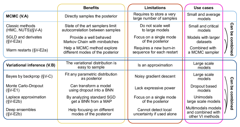
Figure 9: Summary of the different inference approaches used to train a BNN with their benefits, limitations and use cases.

V-E1 Bayes via Dropout

Dropout has initially been proposed as a regularization method [94]. It works by applying multiplicative noise to the target layer. The most commonly used type of noise is Bernoulli noise, but other types such as the Gaussian noise for Gaussian Dropout [94] might be used instead.

Dropout is usually turned off at evaluation time, but leaving it on results in a distribution for the output predictions [95, 96]. It turns out that this procedure, called Monte Carlo Dropout, is in fact variational inference with a variational distribution defined for each weight matrix as:

$$\begin{array}[]{l}\boldsymbol{z}_{i,j}\sim\text{Bernoulli}(p_{i}),\\ \boldsymbol{W}_{i}=\boldsymbol{M}_{i}\cdot\text{diag}(\boldsymbol{z}_{i}),\\ \end{array}$$ (41)

with $\boldsymbol{z}_{i}$ being the random activation coefficients and $\boldsymbol{M}_{i}$ the matrix of weights before dropout is applied. $p_{i}$ is the activation probability for layer $i$ and can be learned or set manually.

When used to train a BNN, dropout should not be seen as a regularization method, as it is part of the variational posterior, not the prior. This means that it should be coupled with a different type of regularization [97], e.g., $\ell^{2}$ weight penalization. The equivalence between the objective function $\mathbf{L}_{\text{dropout}}$ used for training with dropout and $\ell^{2}$ weight regularization, which is defined as:

$$\mathbf{L}_{\text{dropout}}=\dfrac{1}{N}\sum_{D}f(\boldsymbol{y},\boldsymbol{\hat{y}})+\lambda\sum_{\boldsymbol{\theta}}\theta_{i}^{2},$$ (42)

and the ELBO, assuming a normal prior on the weights and the distribution presented in Equation 41 as variational posterior, has been demonstrated in [95]. The argument is similar to the one presented in Section IV-C3.

MC-Dropout is a very convenient technique to perform Bayesian deep learning. It is straightforward to implement and requires little additional knowledge or modeling effort compared to traditional methods. It often leads to a faster training phase compared to other variational inference approaches. If a model has been trained with dropout layers, which are quite widespread in today’s deep learning architectures, and an additional form of regularization acting as prior, it can be used as a BNN without any need to be retrained.

On the other hand, MC-Dropout might lack some expressiveness and may not fully capture the uncertainty associated with the model predictions [98]. It also lacks flexibility compared to other Bayesian methods for online or active learning.

V-E2 Bayes via stochastic gradient descent

Stochastic gradient descent (SGD) and related algorithms are at the core of modern machine learning. The initial goal of SGD is to provide an algorithm that converges to an optimal point estimate solution while having only noisy estimates of the gradient of the objective function. This is especially useful when the training data has to be split into mini-batches. The parameter update rule at time $t$ can be written as:

$$\Delta\boldsymbol{\theta}_{t}=\frac{\epsilon_{t}}{2}\left(\dfrac{N}{n}\nabla\log(p(D_{t,\boldsymbol{y}}|D_{t,\boldsymbol{x}},\boldsymbol{\theta}_{i}))+\nabla\log(p(\boldsymbol{\theta}_{t}))\right),$$ (43)

where $D_{t}$ is a mini-batch subsampled at time $t$ from the complete dataset $D$, $\epsilon_{t}$ is the learning rate at time $t$, $N$ is the size of the whole dataset and $n$ the size of the mini-batch.

SGD, or related optimization algorithms such as ADAM [93], can be reinterpreted as a Markov Chain algorithm [99]. Usually, the hyperparameters of the algorithm are tweaked to ensure that the chain converges to a Dirac distribution, whose position gives the final point estimate. This is done by reducing $\epsilon_{t}$ toward zero while ensuring that $\sum_{t=0}^{\infty}\epsilon_{t}=\infty$. However, if the learning rate is reduced toward a strictly positive value, the underlying Markov Chain will converge to a stationary distribution. If a Bayesian prior is accounted for in the objective function, then this stationary distribution can be an approximation of the corresponding posterior.

MCMC algorithms based on the SGD dynamic

  Draw $\boldsymbol{\theta}_{0}\sim Initial~{}probability~{}distribution$;

  for $t=0$ to $E$ do

     Select a mini-batch $D_{t,\boldsymbol{y}},D_{t,\boldsymbol{x}}\subset D$;

     $f(\boldsymbol{\theta}_{t})=\dfrac{N}{n}\log(p(D_{t,\boldsymbol{y}}|D_{t,\boldsymbol{x}},\boldsymbol{\theta}_{t}))+\log(p(\boldsymbol{\theta}_{t}))$;

     $\Delta_{\boldsymbol{\theta}}f=\text{backprop}_{\boldsymbol{\theta}}(f)$;

     Draw $\eta_{t}\sim\mathcal{N}(0,\epsilon_{t})$;

     $\boldsymbol{\theta}_{t+1}=\boldsymbol{\theta}_{t}-\left(\dfrac{\epsilon_{t}}{2}\Delta_{\theta}f+\eta_{t}\right)$;

  end for

Algorithm 7 Stochastic Gradient Langevin Dynamic (SGLD).

To approximately sample the posterior using the SGD algorithm, a specific MCMC method, called stochastic gradient Langevin dynamic (SGLD) [100], has been developed, see Algorithm 7. Coupling SGD with Langevin dynamic leads to a slightly modified update step:

$$\begin{array}[]{l}\Delta\boldsymbol{\theta}_{t}=\frac{\epsilon_{t}}{2}\left(\dfrac{N}{n}\nabla\log(p(D_{t},\boldsymbol{\theta}_{t}))+\nabla\log(p(\boldsymbol{\theta}_{t}))\right)+\eta_{t},\\ \eta_{t}\sim\mathcal{N}(0,\epsilon_{t}).\end{array}$$ (44)

Welling et al. [100] showed that this method leads to a Markov Chain that samples the posterior if $\epsilon_{t}$ goes toward zero. However, in that case, the successive samples become increasingly autocorrelated. To address this problem, the authors proposed to stop reducing $\epsilon_{t}$ at some point, thus making the samples only an approximation of the posterior. Nevertheless, SGLD offers better theoretical guarantees compared to other MCMC methods when the dataset is split into mini-batches. This makes the algorithm useful in Bayesian deep learning.

To favor the exploration of the posterior, one can use warm restart of the algorithm [101], i.e., restarting the algorithm at a new random position $\boldsymbol{\theta}_{0}$ and with a large learning rate $\epsilon_{0}$. This offers multiple benefits. The main one is to avoid the mode collapse problem [102]. In the case of a BNN, the true Bayesian posterior is usually a complex multimodal distribution, as multiple and sometimes not equivalent parametrizations $\boldsymbol{\theta}$ of the network can fit the training set. Favoring exploration over precise reconstruction can help to achieve a better picture of those different modes. Then, as parameters sampled from the same mode are likely to make the model generalize in a similar manner, using warm restarts enables a much better estimate of the epistemic uncertainty when processing unseen data, even if this approach provides only a very rough approximation of the exact posterior.

Similar to other MCMC methods, this approach still suffers from a huge memory footprint. This is why a number of authors have proposed methods that are more similar to traditional variational inference than to an MCMC algorithm.

Variational Inference based on SGD dynamic

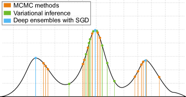
Figure 10: Different techniques for sampling the posterior. MCMC algorithms sample the true posterior but successive samples might be correlated, Variational Inference uses a parametric distribution that can suffer from mode collapse while deep ensembles focus on the modes of the distribution.

Instead of an MCMC algorithm, SGD dynamic can be used as a variational inference method to learn a distribution by using Laplace approximation. Laplace approximation fits a Gaussian posterior by using the maximum a posteriori estimate as the mean and the inverse of the Hessian $\boldsymbol{H}$ of the loss (assuming the loss is the log likelihood) as covariance matrix:

$$p(\boldsymbol{\theta}|D)\approx\mathcal{N}(\boldsymbol{\hat{\theta}},\boldsymbol{H}^{-1}).$$ (45)

Computing $\boldsymbol{H}^{-1}$ is usually intractable for large neural network architectures. Thus, approximations are used, most of the time by analysing the variance of the gradient descent algorithm [88, 89, 103]. However, if those methods are able to capture the fine shape of one mode of the posterior, they cannot fit multiple modes.

Lakshminarayanan et al.  [102] proposed using warm restarts to obtain different point estimate networks instead of fitting a parametric distribution. This method, called deep ensembles; see Figure 10 and Algorithm 8, has been used in the past to perform model averaging. The main contribution of [102] was to show that it enables well-calibrated error estimates. While Lakshminarayanan et al.  [102] claim that their method is non-Bayesian, it has been shown that their approach can still be understood from a Bayesian point of view [12, 104]. When regularization is used, the different point estimates should correspond to modes of a Bayesian posterior. This can be interpreted as approximating the posterior with a distribution parametrized as multiple Dirac deltas, i.e.,

$$q_{\boldsymbol{\phi}}(\boldsymbol{\theta})=\sum_{\boldsymbol{\theta}_{i}\in\boldsymbol{\phi}}\alpha_{\boldsymbol{\theta}_{i}}\delta_{\boldsymbol{\theta}_{i}}(\boldsymbol{\theta}),$$ (46)

with the $\alpha_{\boldsymbol{\theta}_{i}}$ being positive constants such that their sum is equal to one. This approach can be seen as a form of variational inference. Note however that, for a variational distribution containing Dirac deltas, computing the ELBO in a sense that is meaningful for traditional optimization is impossible.

  for $i=0$ to $R$ do

     Draw $\boldsymbol{\theta}_{0}\sim Initial~{}probability~{}distribution$;

     $\epsilon_{t}=\epsilon_{0}$

     for $j=0$ to $N$ do

        $f(\boldsymbol{\theta}_{i,j})=\log(p(D_{\boldsymbol{y}}|D_{\boldsymbol{x}},\boldsymbol{\theta}_{i,j}))+\log(p(\boldsymbol{\theta}_{i,j}))$;

        $\Delta_{\theta}f=\text{backprop}_{\theta}(f)$;

        $\boldsymbol{\theta}_{i}=\boldsymbol{\theta}_{i}-\alpha_{\boldsymbol{\theta}}\Delta_{\theta}f$;

     end for

  end for

Algorithm 8 Deep ensembles.

VI Simplifying Bayesian Neural networks

After training a BNN, one has to use Monte Carlo at evaluation time to estimate uncertainty. This is a major drawback of BNNs. For MCMC-based methods, storing a large set of parametrizations $\Theta$ is also not practical. This section presents mitigation strategies reported in the literature.

VI-A Bayesian inference on the (n-)last layer(s) only

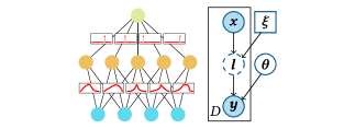
Figure 11: PGM and BNN corresponding to a last-layer model.

The architecture of deep neural networks makes it quite redundant to account for uncertainty for a large number of successive layers. Instead, recent research aims to use only a few stochastic layers, usually positioned at the end of the networks [105, 106]; see Figure 11. With only a few stochastic layers, training and evaluation can be drastically sped up while still obtaining meaningful results from a Bayesian perspective. This approach can be seen as learning a point estimate transformation followed by a shallow BNN.

Training a BNN with some non-stochastic layers is similar to learning the parameters for the prior presented in Section V-D. The weights of the non-Bayesian layers should be considered as both prior and variational-posterior parameters.

VI-B Bayesian teachers

Using a BNN as a teacher is an idea derived from an approach used in Bayesian modeling [107]. The approach is to train a non-stochastic ANN to predict the marginal probability $p(\boldsymbol{y}|\boldsymbol{x},D)$ using a BNN as a teacher [108]. This is related to the idea of knowledge distillation [109, 110] where possibly several pre-trained knowledge sources can be used to train a more functional system.

To do so, the KL-divergence between a parametric distribution $q_{\boldsymbol{\omega}}(\boldsymbol{y}|\boldsymbol{x})$, where $\boldsymbol{\omega}$ are the coefficients of the student network, and $p(\boldsymbol{y}|\boldsymbol{x},D)$ is minimized:

$$\hat{\boldsymbol{\omega}}=\operatorname*{arg\,min}_{\boldsymbol{\omega}}D_{KL}(p(\boldsymbol{y}|\boldsymbol{x},D)||q_{\boldsymbol{\omega}}(\boldsymbol{y}|\boldsymbol{x})).$$ (47)

As this is intractable, Korattikara et al. [108] proposed a Monte Carlo approximation:

$$\hat{\boldsymbol{\omega}}=\operatorname*{arg\,min}_{\boldsymbol{\omega}}-\dfrac{1}{\left|\Theta\right|}\sum_{\boldsymbol{\theta}_{i}\in\Theta}\mathrm{E}_{p(\boldsymbol{y}|\boldsymbol{x},\boldsymbol{\theta}_{i})}\left[\log\left(q_{\boldsymbol{\omega}}(\boldsymbol{y}|\boldsymbol{x})\right)\right].$$ (48)

Here, $\hat{\boldsymbol{\omega}}$ can be estimated using a training dataset $D^{\prime}$ that contains only the features $\boldsymbol{x}$. During training, the probability $p(\boldsymbol{y}|\boldsymbol{x},\boldsymbol{\theta})$ of the labels is given by the teacher BNN. Thus, $D^{\prime}$ can be much larger than $D$. This helps the student network retain the calibration and uncertainty from the teacher.

Menon et al.  [110] observed that, for classification problems, simply using the class probabilities output by a BNN teacher rather than one-hot labels helps the student to retain calibration and uncertainty from the teacher.

A Bayesian teacher can also be used to compress a large set of samples generated using MCMC [111]. Instead of storing $\Theta$, a generative model $G$ (e.g., a GAN in [111]) is trained against the MCMC samples to generate the coefficients $\theta_{i}$ at evaluation time. This approach is similar to variational inference, with G representing a parametric distribution, but the proposed algorithm allows training a much more complex model than the distributions usually considered for variational inference.

VII Performance metrics of Bayesian Neural Networks

One big challenge with BNNs is how to evaluate their performance. They do not directly output a point estimate prediction $\boldsymbol{\hat{y}}$ but a conditional probability distribution $p(\boldsymbol{y}|\boldsymbol{x},D)$, from which an optimal estimate $\boldsymbol{\hat{y}}$ can later be extracted. This means that both the predictive performance, i.e., the ability of the model to give correct answers, and the calibration, i.e., that the network is neither overconfident nor underconfident about its prediction, have to be assessed.

The predictive performance, sometimes called sharpness in statistics, of a network can be assessed by treating the estimator $\boldsymbol{\hat{y}}$ as the prediction. This procedure often depends on the type of data the network is meant to treat. Many different metrics, e.g., mean square error (MSE), $\ell_{n}$ distances and cross-entropy, are used in practice. Covering these metrics is out of the scope of this tutorial. Instead, we refer the reader to [112] for more details.

The standard method to assess the model calibration is a calibration curve, also called a reliability diagram [32, 113]. It is defined as a function $\check{p}:[0,1]\rightarrow[0,1]$ that represents the observed probability $\check{p}$, or empirical frequency, as a function of the predicted probability $\hat{p}$; see Figure 12. If $\check{p}<\hat{p}$, then the model is overconfident. Otherwise, it is underconfident. A well-calibrated model should have $\check{p}\cong\hat{p}$. Using this approach requires to first choose a set of events $\mathcal{E}$ with different predicted probabilities and then to measure the empirical frequency of each event using a test set $T$.

For a binary classifier, the set of test events can be chosen as the set of all sets of datapoints with predicted probabilities of acceptance in interval $[p-\delta,p+\delta]$ for a chosen $\delta$, or alternatively $[0,p]$ or $[1-p,1]$ for small datasets. The empirical frequency is given by:

$$\check{p}=\dfrac{\sum_{\boldsymbol{\check{y}}\in T_{\boldsymbol{y}}}\boldsymbol{\check{y}}\cdot\mathbb{I}_{[\hat{p}-\delta,\hat{p}+\delta]}(\boldsymbol{\hat{y}})}{\sum_{\boldsymbol{\check{y}}\in T_{\boldsymbol{y}}}\mathbb{I}_{[\hat{p}-\delta,\hat{p}+\delta]}(\boldsymbol{\hat{y}})}.$$ (49)

For multiclass classifiers, the calibration curve can be independently checked for each class against all the other classes. In this case, the problem is reduced to a binary classifier.

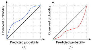
Figure 12: Examples of calibration curves for underconfident (a) and overconfident (b) models.

Regression problems are slightly more complex since the network does not output a confidence level, as in a classifier, but a distribution of possible outputs. The solution is to use an intermediate statistic with a known probability distribution. Assuming independence between the $\boldsymbol{\hat{y}}$ for a sufficiently large set of different randomly selected inputs $\boldsymbol{x}$, one can assume that the normalized sum of squared residuals (NSSR) follows a Chi-square law:

$$\text{NSSR}=(\boldsymbol{\hat{y}}-\boldsymbol{\check{y}})^{\intercal}\boldsymbol{\Sigma}_{\boldsymbol{\hat{y}}}^{-1}(\boldsymbol{\hat{y}}-\boldsymbol{\check{y}})\sim\chi_{Dim(\boldsymbol{y})}^{2}.$$ (50)

This allows attributing to each data point in the test set $T$ a predicted probability that is the probability of observing a variance-normalized distance between the prediction and the true value equal to or lower than the measured NSSR. Formally, the predicted probability is computed as:

$$\hat{p}_{i}=X_{\text{Dim}(\boldsymbol{y})}^{2}\left(\text{NSSR}\right)\quad\forall(\boldsymbol{y}_{i},\boldsymbol{x}_{i})\in T,$$ (51)

where $X_{\text{Dim}(\boldsymbol{y})}^{2}$ is the Chi-square cumulative distribution, with $\text{Dim}(\boldsymbol{y})$ degrees of freedom. The observed probability can be computed as:

$$\check{p}_{i}=\dfrac{1}{|T|}\sum_{j=1}^{|T|}\mathbb{I}_{[0,\infty)}(\hat{p}_{j}-\hat{p}_{i}).$$ (52)

We present in the Supplementary Material a practical computation of such calibration curve for the sparse measure practical example (Practical example II).

Giving the whole calibration curve for a given stochastic model allows observing where the model is likely to be overconfident or underconfident. It also allows, to a certain extent, to recalibrate the model [113]. However, providing a summary measure to ease comparison or interpretation might also be necessary. The area under the curve (AUC) is a standard metric of the form:

$$\text{AUC}=\int_{0}^{1}\check{p}d\hat{p}.$$ (53)

An AUC of $0.5$ indicates that the model is, on average, well calibrated.

The distance from the actual calibration curve to the ideal calibration curve is also a good indicator for the calibration of a model:

$$d(\check{p},\hat{p})=\sqrt{\int_{0}^{1}(\check{p}-\hat{p})^{2}d\hat{p}}.$$ (54)

When $d(\check{p},\hat{p})=0$, then the model is perfectly calibrated.

Other measures have also been proposed. Examples include the expected calibration error and some discretized variants of the distance from the actual calibration curve to the ideal calibration curve [16].

VIII Conclusion

This tutorial covers the design, training and evaluation of BNNs. While their underlying principle is simple, i.e., just training an ANN with some probability distribution attached to its weights, designing efficient algorithms remains very challenging. Nonetheless, the potential applications of BNNs are huge. In particular, BNNs constitute a promising paradigm allowing the application of deep learning in areas where a system is not allowed to fail to generalize without emitting a warning. Finally, Bayesian methods can help design new learning and regularization strategies. Thus, their relevance extends to traditional point estimate models.

Online resources for the tutorial: https://github.com/french-paragon/BayesianNeuralNetwork-Tutorial-Metarepos Supplementary material, as well as additional practical examples for the covered material with the corresponding source code implementation, have been provided.

IX Acknowledgments

This material is partially based on research sponsored by the Australian Research Council https://www.arc.gov.au/ (Grants DP150100294 and DP150104251), and Air Force Research Laboratory and DARPA https://afrl.dodlive.mil/tag/darpa/ under agreement number FA8750-19-2-0501.

Appendix A Implementing parameter-efficient normal distributions for variational inference

Given a random vector $\boldsymbol{\varepsilon}$ in which each independent and identically distributed component follows a standard normal distribution $\mathcal{N}(0,1)$, one can obtain a sample $\boldsymbol{\theta}$ from a normal distribution $\mathcal{N}(\boldsymbol{\mu},\boldsymbol{\Sigma})$ using the following formulas:

$$\boldsymbol{\theta}=\sqrt{\boldsymbol{\Sigma}}\boldsymbol{\varepsilon}+\boldsymbol{\mu},$$ (55)

where $\sqrt{\boldsymbol{\Sigma}}$ is a matrix such that $\sqrt{\boldsymbol{\Sigma}}\sqrt{\boldsymbol{\Sigma}}^{\top}=\boldsymbol{\Sigma}$. When a variational inference algorithm needs to learn the covariance matrix of $\boldsymbol{\theta}$, it is often more convenient to learn $\sqrt{\boldsymbol{\Sigma}}$. Assuming $\boldsymbol{\theta}$ has $n$ entries, $\sqrt{\boldsymbol{\Sigma}}\sqrt{\boldsymbol{\Sigma}}^{\top}$ is the Cholesky decomposition of $\boldsymbol{\Sigma}$. As such, $\sqrt{\boldsymbol{\Sigma}}$ is a lower triangular matrix and $\mathcal{O}(n^{2})$ variational parameters are required to learn the exact covariance matrix. This becomes exceedingly computationally expensive rather quickly when $n$ becomes large.

A straightforward simplification is to only consider a diagonal approximation of $\boldsymbol{\Sigma}$. This can be enforced by learning only the diagonal coefficients of $\sqrt{\boldsymbol{\Sigma}}$, meaning only $\mathcal{O}(n)$ variational parameters are required (Figure 13a). This approach can be extended to learn more correlation coefficients by learning a block diagonal [88] covariance matrix, which can be done by learning the corresponding lower triangular entries in $\sqrt{\boldsymbol{\Sigma}}$ (Figure 13b). If the maximal size of the nonzero blocks is fixed to be $w$, $\mathcal{O}(w\cdot n)$ variational parameters are required. The major drawback of this model is that the index of two given parameters determines whether their covariance can be learned by the variational distribution. This is not always ideal, as it is hard to predict which parameters will be the most correlated and need to be positioned close to one another. An alternative is to learn a diagonal plus low rank approximation of $\boldsymbol{\Sigma}$ [89]. This is done by sampling a vector $\boldsymbol{\varepsilon}$ with $n+r$ (instead of $n$) components. $\sqrt{\boldsymbol{\Sigma}}$ is then defined as:

$$\sqrt{\boldsymbol{\Sigma}}=\left[D,~{}L\right],$$ (56)

where $D$ is a diagonal matrix of size $n\times n$ and $L$ is a lower triangular matrix of size $n\times r$ (Figure 13c). This means that the model has more flexibility to learn the correlation between all the components of $\boldsymbol{\theta}$ while only requiring $\mathcal{O}(n\cdot r)$ variational parameters.

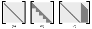
Figure 13: Nonzero entries in $\sqrt{\boldsymbol{\Sigma}}$ when learning a diagonal (a), block diagonal (b) or diagonal plus low rank (c) approximation of $\boldsymbol{\Sigma}$

Appendix B A proof of Equation 38

Let us assume that we have a probability space $(\Omega,\mathcal{F},\operatorname{P})$, where $\Omega$ is a set of outcomes, $\mathcal{F}$ is a $\sigma$-algebra of $\Omega$ representing possible events and $\operatorname{P}$ is a measure defined on $\mathcal{F}$ and which assigns a value of $1$ to $\Omega$, representing the probability of an event. In addition, assume that we have a probability distribution $q_{\phi}(\boldsymbol{\theta})$ for a given random variable $\boldsymbol{\theta}$, a probability distribution $q(\varepsilon)$ for a given random variable $\varepsilon$ and a functional relation $t(\varepsilon,\boldsymbol{\phi})$ such that $t(\varepsilon,\boldsymbol{\phi})$ is distributed according to $q_{\phi}(\boldsymbol{\theta})$ and $t(\varepsilon,\boldsymbol{\phi})$ is a bijection with respect to $\varepsilon$. Thus, we have:

$$\small\operatorname{P}(\boldsymbol{\theta}^{-1}(t(E,\boldsymbol{\phi})))=\operatorname{P}(\varepsilon^{-1}(E))\quad\forall E\in\varepsilon(\mathcal{F}),$$ (57)

with

$$\begin{array}[]{c}\varepsilon(\mathcal{F})=\left\{\{\varepsilon(\omega):\omega\in e\}:e\in\mathcal{F}\right\},\\ \\ t(E,\boldsymbol{\phi})=\{t(\varepsilon,\boldsymbol{\phi}):\varepsilon\in E\},\\ \\ \varepsilon^{-1}(E)=\bigcup_{e\in\mathcal{F}\land\varepsilon(e)\subseteq E}e,\\ \\ \boldsymbol{\theta}^{-1}(t(E,\boldsymbol{\phi}))=\bigcup_{e\in\mathcal{F}\land\boldsymbol{\theta}(e)\subseteq t(E,\boldsymbol{\phi})}e.\end{array}$$

Since $t(\varepsilon,\boldsymbol{\phi})$ is a bijection with respect to $\varepsilon$, we have $\varepsilon^{-1}(E)=\boldsymbol{\theta}^{-1}(t(E,\boldsymbol{\phi}))$. This implies:

$$\small\int_{\boldsymbol{\theta}\in t(E,\boldsymbol{\phi})}q_{\phi}(\boldsymbol{\theta})d\boldsymbol{\theta}=\int_{\varepsilon\in E}q(\varepsilon)d\varepsilon\quad\forall E\in\varepsilon(\mathcal{F}).$$ (58)

which in turn implies:

$$\small q_{\phi}(\boldsymbol{\theta})d\boldsymbol{\theta}=q(\varepsilon)d\varepsilon$$ (59)

for non-degenerated probability distributions $q_{\phi}(\boldsymbol{\theta})$ and $q(\varepsilon)$.

Now, given a differentiable function $f(\boldsymbol{\phi},\boldsymbol{\theta})$, we have:

$$\small\int_{\boldsymbol{\theta}\in t(\varepsilon(\Omega),\boldsymbol{\phi})}f(\boldsymbol{\phi},\boldsymbol{\theta})q_{\phi}(\boldsymbol{\theta})d\boldsymbol{\theta}=\int_{\varepsilon\in\varepsilon(\Omega)}f(\boldsymbol{\phi},t(\varepsilon,\boldsymbol{\phi}))q(\varepsilon)d\varepsilon$$ (60)

which implies Equation (38).

References

- [1] C. Szegedy, W. Zaremba, I. Sutskever, J. Bruna, D. Erhan, I. Goodfellow, and R. Fergus, “Intriguing properties of neural networks,” arXiv preprint arXiv:1312.6199, 2013.
- [2] Q. Rao and J. Frtunikj, “Deep learning for self-driving cars: Chances and challenges,” in Proceedings of the 1st International Workshop on Software Engineering for AI in Autonomous Systems, ser. SEFAIS ’18, 2018, pp. 35–38.
- [3] J. Ker, L. Wang, J. Rao, and T. Lim, “Deep learning applications in medical image analysis,” IEEE Access, vol. 6, pp. 9375–9389, 2018.
- [4] R. C. Cavalcante, R. C. Brasileiro, V. L. Souza, J. P. Nobrega, and A. L. Oliveira, “Computational intelligence and financial markets: A survey and future directions,” Expert Systems with Applications, vol. 55, pp. 194–211, 2016.
- [5] H. M. D. Kabir, A. Khosravi, M. A. Hosen, and S. Nahavandi, “Neural network-based uncertainty quantification: A survey of methodologies and applications,” IEEE Access, vol. 6, pp. 36 218–36 234, 2018.
- [6] A. Etz, Q. F. Gronau, F. Dablander, P. A. Edelsbrunner, and B. Baribault, “How to become a Bayesian in eight easy steps: An annotated reading list,” Psychonomic Bulletin & Review, vol. 25, pp. 219–234, 2018.
- [7] N. G. Polson, V. Sokolov et al., “Deep learning: a Bayesian perspective,” Bayesian Analysis, vol. 12, no. 4, pp. 1275–1304, 2017.
- [8] J. Lampinen and A. Vehtari, “Bayesian approach for neural networks—review and case studies,” Neural Networks, vol. 14, no. 3, pp. 257 – 274, 2001.
- [9] D. M. Titterington, “Bayesian methods for neural networks and related models,” Statist. Sci., vol. 19, no. 1, pp. 128–139, 02 2004.
- [10] E. Goan and C. Fookes, Bayesian Neural Networks: An Introduction and Survey. Cham: Springer International Publishing, 2020, pp. 45–87.
- [11] H. Wang and D.-Y. Yeung, “A survey on bayesian deep learning,” ACM Comput. Surv., vol. 53, no. 5, Sep. 2020.
- [12] A. G. Wilson and P. Izmailov, “Bayesian deep learning and a probabilistic perspective of generalization,” CoRR, vol. abs/2002.08791, 2020. [Online]. Available: http://arxiv.org/abs/2002.08791
- [13] I. Goodfellow, Y. Bengio, and A. Courville, Deep Learning. MIT Press, 2016, http://www.deeplearningbook.org.
- [14] S. C.-H. Yang, W. K. Vong, R. B. Sojitra, T. Folke, and P. Shafto, “Mitigating belief projection in explainable artificial intelligence via bayesian teaching,” Scientific Reports, vol. 11, no. 1, p. 9863, May 2021.
- [15] C. Guo, G. Pleiss, Y. Sun, and K. Q. Weinberger, “On calibration of modern neural network,” in Proceedings of the 34th International Conference on Machine Learning - Volume 70, ser. ICML’17, 2017, pp. 1321–1330.
- [16] J. Nixon, M. W. Dusenberry, L. Zhang, G. Jerfel, and D. Tran, “Measuring calibration in deep learning,” in The IEEE Conference on Computer Vision and Pattern Recognition (CVPR) Workshops, June 2019.
- [17] D. Hendrycks and K. Gimpel, “A baseline for detecting misclassified and out-of-distribution examples in neural networks,” in 5th International Conference on Learning Representations, ICLR 2017, Conference Track Proceedings, 2017.
- [18] Z.-H. Zhou, Ensemble Methods: Foundations and Algorithms, 1st ed. Chapman and Hall/CRC, 2012.
- [19] F. Galton, “Vox Populi,” Nature, vol. 75, no. 1949, pp. 450–451, Mar 1907.
- [20] L. Breiman, “Bagging predictors,” Machine Learning, vol. 24, no. 2, pp. 123–140, Aug 1996.
- [21] D. J. C. MacKay, “A practical Bayesian framework for backpropagation networks,” Neural Computation, vol. 4, no. 3, pp. 448–472, 1992.
- [22] P. Izmailov, S. Vikram, M. D. Hoffman, and A. G. Wilson, “What are Bayesian neural network posteriors really like?” CoRR, vol. abs/2104.14421, 2021. [Online]. Available: http://arxiv.org/abs/2104.14421
- [23] Y. Gal and Z. Ghahramani, “Bayesian convolutional neural networks with Bernoulli approximate variational inference,” in 4th International Conference on Learning Representations (ICLR) workshop track, 2016.
- [24] D. P. Kingma and M. Welling, “Stochastic gradient vb and the variational auto-encoder,” in Second International Conference on Learning Representations, ICLR, vol. 19, 2014.
- [25] C. Robert, The Bayesian choice: from decision-theoretic foundations to computational implementation. Springer Science & Business Media, 2007.
- [26] J. Mitros and B. M. Namee, “On the validity of Bayesian neural networks for uncertainty estimation,” in AICS, 2019.
- [27] A. Kristiadi, M. Hein, and P. Hennig, “Being Bayesian, even just a bit, fixes overconfidence in ReLU networks,” CoRR, vol. abs/2002.10118, 2020. [Online]. Available: http://arxiv.org/abs/2002.10118
- [28] Y. Ovadia, E. Fertig, J. Ren, Z. Nado, D. Sculley, S. Nowozin, J. Dillon, B. Lakshminarayanan, and J. Snoek, “Can you trust your model's uncertainty? evaluating predictive uncertainty under dataset shift,” in Advances in Neural Information Processing Systems 32. Curran Associates, Inc., 2019, pp. 13 991–14 002.
- [29] A. D. Kiureghian and O. Ditlevsen, “Aleatory or epistemic? does it matter?” Structural Safety, vol. 31, no. 2, pp. 105–112, 2009, risk Acceptance and Risk Communication.
- [30] S. Depeweg, J.-M. Hernandez-Lobato, F. Doshi-Velez, and S. Udluft, “Decomposition of uncertainty in Bayesian deep learning for efficient and risk-sensitive learning,” in Proceedings of the 35th International Conference on Machine Learning, ser. Proceedings of Machine Learning Research, vol. 80, 2018, pp. 1184–1193.
- [31] D. H. Wolpert, “The lack of a priori distinctions between learning algorithms,” Neural Computation, vol. 8, no. 7, pp. 1341–1390, 1996.
- [32] A. Kendall and Y. Gal, “What uncertainties do we need in Bayesian deep learning for computer vision?” in Proceedings of the 31st International Conference on Neural Information Processing Systems, ser. NIPS’17, 2017, p. 5580–5590.
- [33] T. Auld, A. W. Moore, and S. F. Gull, “Bayesian neural networks for internet traffic classification,” IEEE Transactions on Neural Networks, vol. 18, no. 1, pp. 223–239, 2007.
- [34] X. Zhang and S. Mahadevan, “Bayesian neural networks for flight trajectory prediction and safety assessment,” Decision Support Systems, vol. 131, p. 113246, 2020.
- [35] S. Arangio and F. Bontempi, “Structural health monitoring of a cable–stayed bridge with Bayesian neural networks,” Structure and Infrastructure Engineering, vol. 11, no. 4, pp. 575–587, 2015.
- [36] S. M. Bateni, D.-S. Jeng, and B. W. Melville, “Bayesian neural networks for prediction of equilibrium and time-dependent scour depth around bridge piers,” Advances in Engineering Software, vol. 38, no. 2, pp. 102–111, 2007.
- [37] X. Zhang, F. Liang, R. Srinivasan, and M. Van Liew, “Estimating uncertainty of streamflow simulation using bayesian neural networks,” Water Resources Research, vol. 45, no. 2, 2009.
- [38] A. D. Cobb, M. D. Himes, F. Soboczenski, S. Zorzan, M. D. O’Beirne, A. G. Baydin, Y. Gal, S. D. Domagal-Goldman, G. N. Arney, and D. A. and, “An ensemble of bayesian neural networks for exoplanetary atmospheric retrieval,” The Astronomical Journal, vol. 158, no. 1, p. 33, jun 2019.
- [39] F. Aminian and M. Aminian, “Fault diagnosis of analog circuits using Bayesian neural networks with wavelet transform as preprocessor,” Journal of Electronic Testing, vol. 17, no. 1, pp. 29–36, Feb 2001.
- [40] W. Beker, A. Wołos, S. Szymkuć, and B. A. Grzybowski, “Minimal–uncertainty prediction of general drug–likeness based on Bayesian neural networks,” Nature Machine Intelligence, vol. 2, no. 8, pp. 457–465, Aug 2020.
- [41] Y. Gal, R. Islam, and Z. Ghahramani, “Deep Bayesian active learning with image data,” in Proceedings of the 34th International Conference on Machine Learning - Volume 70, ser. ICML’17, 2017, p. 1183–1192.
- [42] T. Tran, T.-T. Do, I. Reid, and G. Carneiro, “Bayesian generative active deep learning,” CoRR, vol. abs/1904.11643, 2019. [Online]. Available: http://arxiv.org/abs/1904.11643
- [43] M. Opper and O. Winther, “A Bayesian approach to on-line learning,” On-line learning in neural networks, pp. 363–378, 1998.
- [44] H. Ritter, A. Botev, and D. Barber, “Online structured Laplace approximations for overcoming catastrophic forgetting,” in Proceedings of the 32nd International Conference on Neural Information Processing Systems, ser. NIPS’18, 2018, pp. 3742–3752.
- [45] S. Pouyanfar, S. Sadiq, Y. Yan, H. Tian, Y. Tao, M. P. Reyes, M.-L. Shyu, S.-C. Chen, and S. S. Iyengar, “A survey on deep learning: Algorithms, techniques, and applications,” ACM Comput. Surv., vol. 51, no. 5, Sep. 2018.
- [46] W. L. Buntine, “Operations for learning with graphical models,” Journal of Artificial Intelligence Research, vol. 2, pp. 159–225, Dec 1994.
- [47] Y. Wen, P. Vicol, J. Ba, D. Tran, and R. Grosse, “Flipout: Efficient pseudo-independent weight perturbations on mini-batches,” in International Conference on Learning Representations, 2018.
- [48] C. Zhang, S. Bengio, M. Hardt, B. Recht, and O. Vinyals, “Understanding deep learning requires rethinking generalization,” in 5th International Conference on Learning Representations, ICLR, 2017.
- [49] B. Carpenter, A. Gelman, M. D. Hoffman, D. Lee, B. Goodrich, M. Betancourt, M. Brubaker, J. Guo, P. Li, and A. Riddell, “Stan: A probabilistic programming language,” Journal of statistical software, vol. 76, no. 1, 2017.
- [50] A. Gelman and other Stan developers, “Prior choice recommendations,” 2020, retrieved from https://github.com/stan-dev/stan/wiki/Prior-Choice-Recommendations [last seen 13.07.2020].
- [51] D. Silvestro and T. Andermann, “Prior choice affects ability of Bayesian neural networks to identify unknowns,” CoRR, vol. abs/2005.04987, 2020. [Online]. Available: http://arxiv.org/abs/2005.04987
- [52] K. P. Murphy, Machine Learning: A Probabilistic Perspective. The MIT Press, 2012.
- [53] A. A. Pourzanjani, R. M. Jiang, B. Mitchell, P. J. Atzberger, and L. R. Petzold, “Bayesian inference over the Stiefel manifold via the Givens representation,” CoRR, vol. abs/1710.09443, 2017. [Online]. Available: http://arxiv.org/abs/1710.09443
- [54] J. L. Ba, J. R. Kiros, and G. E. Hinton, “Layer normalization,” CoRR, vol. arXiv:1607.06450, 2016, in NIPS 2016 Deep Learning Symposium.
- [55] G.-J. Qi and J. Luo, “Small data challenges in big data era: A survey of recent progress on unsupervised and semi-supervised methods,” CoRR, vol. abs/1903.11260, 2019. [Online]. Available: http://arxiv.org/abs/1903.11260
- [56] N. Natarajan, I. S. Dhillon, P. K. Ravikumar, and A. Tewari, “Learning with noisy labels,” in Advances in Neural Information Processing Systems 26. Curran Associates, Inc., 2013, pp. 1196–1204.
- [57] B. Frenay and M. Verleysen, “Classification in the presence of label noise: A survey,” IEEE Transactions on Neural Networks and Learning Systems, vol. 25, no. 5, pp. 845–869, 2014.
- [58] A. C. Tommi and T. Jaakkola, “On information regularization,” in In Proceedings of the 19th UAI, 2003.
- [59] K. Sohn, D. Berthelot, C.-L. Li, Z. Zhang, N. Carlini, E. D. Cubuk, A. Kurakin, H. Zhang, and C. Raffel, “FixMatch: Simplifying semi-supervised learning with consistency and confidence,” CoRR, vol. abs/2001.07685, 2020. [Online]. Available: https://arxiv.org/abs/2001.07685
- [60] M. Belkin, P. Niyogi, and V. Sindhwani, “Manifold regularization: A geometric framework for learning from labeled and unlabeled examples,” J. Mach. Learn. Res., vol. 7, pp. 2399–2434, Dec. 2006.
- [61] S. Yu, B. Krishnapuram, R. Rosales, and R. B. Rao, “Bayesian co-training,” Journal of Machine Learning Research, vol. 12, no. 80, pp. 2649–2680, 2011.
- [62] R. Kunwar, U. Pal, and M. Blumenstein, “Semi-supervised online Bayesian network learner for handwritten characters recognition,” in 2014 22nd International Conference on Pattern Recognition, 2014, pp. 3104–3109.
- [63] D.-H. Lee, “Pseudo-label: The simple and efficient semi-supervised learning method for deep neural networks,” in Workshop on challenges in representation learning, ICML, vol. 3, 2013.
- [64] Z. Li, B. Ko, and H.-J. Choi, “Naive semi-supervised deep learning using pseudo-label,” Peer-to-Peer Networking and Applications, vol. 12, no. 5, pp. 1358–1368, 2019.
- [65] M. S. Bari, M. T. Mohiuddin, and S. Joty, “MultiMix: A robust data augmentation strategy for cross-lingual nlp,” in ICML, 2020.
- [66] O. Chapelle, J. Weston, L. Bottou, and V. Vapnik, “Vicinal risk minimization,” in Advances in Neural Information Processing Systems 13. MIT Press, 2001, pp. 416–422.
- [67] Q. Xie, Z. Dai, E. H. Hovy, M. Luong, and Q. V. Le, “Unsupervised data augmentation,” CoRR, vol. abs/1904.12848, 2019. [Online]. Available: http://arxiv.org/abs/1904.12848
- [68] T. Hospedales, A. Antoniou, P. Micaelli, and A. Storkey, “Meta-learning in neural networks: A survey,” CoRR, vol. abs/2004.05439, 2020. [Online]. Available: http://arxiv.org/abs/2004.05439
- [69] S. J. Pan and Q. Yang, “A survey on transfer learning,” IEEE Transactions on Knowledge and Data Engineering, vol. 22, no. 10, pp. 1345–1359, 2010.
- [70] X. Qiu, T. Sun, Y. Xu, Y. Shao, N. Dai, and X. Huang, “Pre-trained models for natural language processing: A survey,” CoRR, vol. abs/2003.08271, 2020.
- [71] L. Jing and Y. Tian, “Self-supervised visual feature learning with deep neural networks: A survey,” IEEE Transactions on Pattern Analysis and Machine Intelligence, pp. 1–1, 2020.
- [72] X.-F. Han, H. Laga, and M. Bennamoun, “Image-based 3d object reconstruction: State-of-the-art and trends in the deep learning era,” IEEE transactions on pattern analysis and machine intelligence, vol. 43, no. 5, pp. 1578–1604, 2021.
- [73] H. Laga, L. V. Jospin, F. Boussaid, and M. Bennamoun, “A survey on deep learning techniques for stereo-based depth estimation,” IEEE Transactions on Pattern Analysis and Machine Intelligence, 2020.
- [74] E. Grant, C. Finn, S. Levine, T. Darrell, and T. L. Griffiths, “Recasting gradient-based meta-learning as hierarchical Bayes,” in 6th International Conference on Learning Representations, ICLR 2018, Vancouver, BC, Canada, April 30 - May 3, 2018, Conference Track Proceedings, 2018.
- [75] L. Beyer, X. Zhai, A. Oliver, and A. Kolesnikov, “S4L: Self-supervised semi-supervised learning,” in 2019 IEEE/CVF International Conference on Computer Vision (ICCV), 2019, pp. 1476–1485.
- [76] W. K. Hastings, “Monte Carlo sampling methods using Markov chains and their applications,” Biometrika, vol. 57, no. 1, pp. 97–109, 04 1970.
- [77] D. M. Blei, A. Kucukelbir, and J. D. McAuliffe, “Variational inference: A review for statisticians,” Journal of the American Statistical Association, vol. 112, no. 518, pp. 859–877, 2017.
- [78] R. Bardenet, A. Doucet, and C. Holmes, “On Markov Chain Monte Carlo methods for tall data,” J. Mach. Learn. Res., vol. 18, no. 1, pp. 1515–1557, Jan. 2017.
- [79] E. I. George, G. Casella, and E. I. George, “Explaining the Gibbs sampler,” The American Statistician, 1992.
- [80] S. Chib and E. Greenberg, “Understanding the Metropolis-Hastings algorithm,” The American Statistician, vol. 49, no. 4, pp. 327–335, 1995.
- [81] R. M. Neal et al., “MCMC using Hamiltonian dynamics,” Handbook of Markov Chain Monte Carlo, vol. 2, no. 11, p. 2, 2011.
- [82] M. D. Hoffman and A. Gelman, “The No-U-Turn sampler: adaptively setting path lengths in Hamiltonian Monte Carlo,” Journal of Machine Learning Research, vol. 15, no. 1, pp. 1593–1623, 2014.
- [83] S. Kullback and R. A. Leibler, “On information and sufficiency,” The Annals of Mathematical Statistics, vol. 22, no. 1, pp. 79 – 86, 1951.
- [84] C. E. Shannon, “A mathematical theory of communication,” The Bell System Technical Journal, vol. 27, no. 3, pp. 379–423, 1948.
- [85] M. D. Hoffman, D. M. Blei, C. Wang, and J. Paisley, “Stochastic variational inference,” J. Mach. Learn. Res., vol. 14, no. 1, pp. 1303–1347, May 2013.
- [86] A. Graves, “Practical variational inference for neural networks,” in Advances in Neural Information Processing Systems 24. Curran Associates, Inc., 2011, pp. 2348–2356.
- [87] Z. Ghahramani and M. J. Beal, “Propagation algorithms for variational Bayesian learning,” in Advances in Neural Information Processing Systems 13. MIT Press, 2001, pp. 507–513.
- [88] H. Ritter, A. Botev, and D. Barber, “A scalable laplace approximation for neural networks,” in International Conference on Learning Representations, 2018.
- [89] W. J. Maddox, P. Izmailov, T. Garipov, D. P. Vetrov, and A. G. Wilson, “A simple baseline for Bayesian uncertainty in deep learning,” in Advances in Neural Information Processing Systems 32. Curran Associates, Inc., 2019, pp. 13 153–13 164.
- [90] J. M. Hernández-Lobato and R. P. Adams, “Probabilistic backpropagation for scalable learning of Bayesian neural networks,” in Proceedings of the 32nd International Conference on International Conference on Machine Learning - Volume 37, ser. ICML’15, 2015, p. 1861–1869.
- [91] C. Blundell, J. Cornebise, K. Kavukcuoglu, and D. Wierstra, “Weight uncertainty in neural network,” in Proceedings of the 32nd International Conference on Machine Learning, ser. Proceedings of Machine Learning Research, vol. 37, 2015, pp. 1613–1622.
- [92] D. P. Kingma, M. Welling et al., “An introduction to variational autoencoders,” Foundations and Trends® in Machine Learning, vol. 12, no. 4, pp. 307–392, 2019.
- [93] D. Kingma and J. Ba, “Adam: A method for stochastic optimization,” International Conference on Learning Representations, 12 2014.
- [94] N. Srivastava, G. Hinton, A. Krizhevsky, I. Sutskever, and R. Salakhutdinov, “Dropout: A simple way to prevent neural networks from overfitting,” Journal of Machine Learning Research, vol. 15, no. 56, pp. 1929–1958, 2014.
- [95] Y. Gal and Z. Ghahramani, “Dropout as a Bayesian approximation: Representing model uncertainty in deep learning,” in Proceedings of the 33rd International Conference on Machine Learning - Volume 48, ser. ICML’16, 2016, p. 1050–1059.
- [96] Y. Li and Y. Gal, “Dropout inference in Bayesian neural networks with alpha-divergences,” in Proceedings of the 34th International Conference on Machine Learning - Volume 70, ser. ICML’17, 2017, pp. 2052–2061.
- [97] J. Hron, A. Matthews, and Z. Ghahramani, “Variational Bayesian dropout: pitfalls and fixes,” in Proceedings of the 35th International Conference on Machine Learning, ser. Proceedings of Machine Learning Research, vol. 80, 2018, pp. 2019–2028.
- [98] A. Chan, A. Alaa, Z. Qian, and M. Van Der Schaar, “Unlabelled data improves Bayesian uncertainty calibration under covariate shift,” in Proceedings of the 37th International Conference on Machine Learning, ser. Proceedings of Machine Learning Research, vol. 119. Virtual: PMLR, 13–18 Jul 2020, pp. 1392–1402.
- [99] S. Mandt, M. D. Hoffman, and D. M. Blei, “Stochastic gradient descent as approximate Bayesian inference,” The Journal of Machine Learning Research, vol. 18, no. 1, pp. 4873–4907, 2017.
- [100] M. Welling and Y. W. Teh, “Bayesian learning via stochastic gradient Langevin dynamics,” in Proceedings of the 28th international conference on machine learning, ser. ICML ’11, 2011, pp. 681–688.
- [101] N. Seedat and C. Kanan, “Towards calibrated and scalable uncertainty representations for neural networks,” CoRR, vol. abs/1911.00104, 2019. [Online]. Available: http://arxiv.org/abs/1911.00104
- [102] B. Lakshminarayanan, A. Pritzel, and C. Blundell, “Simple and scalable predictive uncertainty estimation using deep ensembles,” in Advances in Neural Information Processing Systems 30. Curran Associates, Inc., 2017, pp. 6402–6413.
- [103] M. Khan, D. Nielsen, V. Tangkaratt, W. Lin, Y. Gal, and A. Srivastava, “Fast and scalable Bayesian deep learning by weight-perturbation in Adam,” in Proceedings of the 35th International Conference on Machine Learning, ser. Proceedings of Machine Learning Research, vol. 80, 2018, pp. 2611–2620.
- [104] T. Pearce, F. Leibfried, A. Brintrup, M. Zaki, and A. Neely, “Uncertainty in neural networks: Approximately Bayesian ensembling,” in AISTATS 2020, 2020.
- [105] J. Zeng, A. Lesnikowski, and J. M. Alvarez, “The relevance of Bayesian layer positioning to model uncertainty in deep Bayesian active learning,” CoRR, vol. abs/1811.12535, 2018. [Online]. Available: http://arxiv.org/abs/1811.12535
- [106] N. Brosse, C. Riquelme, A. Martin, S. Gelly, and Éric Moulines, “On last-layer algorithms for classification: Decoupling representation from uncertainty estimation,” CoRR, vol. abs/2001.08049, 2020. [Online]. Available: http://arxiv.org/abs/2001.08049
- [107] E. Snelson and Z. Ghahramani, “Compact approximations to Bayesian predictive distributions,” in Proceedings of the 22nd International Conference on Machine Learning, ser. ICML ’05, 2005, p. 840–847.
- [108] A. Korattikara, V. Rathod, K. Murphy, and M. Welling, “Bayesian dark knowledge,” in Proceedings of the 28th International Conference on Neural Information Processing Systems - Volume 2, ser. NIPS’15, 2015, pp. 3438–3446.
- [109] G. Hinton, O. Vinyals, and J. Dean, “Distilling the knowledge in a neural network,” arXiv preprint arXiv:1503.02531, 2015, in NIPS 2014 Deep Learning Workshop.
- [110] A. K. Menon, A. S. Rawat, S. J. Reddi, S. Kim, and S. Kumar, “Why distillation helps: a statistical perspective,” CoRR, vol. abs/2005.10419, 2020. [Online]. Available: https://arxiv.org/abs/2005.10419
- [111] K.-C. Wang, P. Vicol, J. Lucas, L. Gu, R. Grosse, and R. Zemel, “Adversarial distillation of Bayesian neural network posteriors,” in Proceedings of the 35th International Conference on Machine Learning, ser. Proceedings of Machine Learning Research, vol. 80, 2018, pp. 5190–5199.
- [112] K. Janocha and W. M. Czarnecki, “On loss functions for deep neural networks in classification,” Schedae Informaticae, vol. 1/2016, 2017. [Online]. Available: http://dx.doi.org/10.4467/20838476SI.16.004.6185
- [113] V. Kuleshov, N. Fenner, and S. Ermon, “Accurate uncertainties for deep learning using calibrated regression,” in Proceedings of the 35th International Conference on Machine Learning, ser. Proceedings of Machine Learning Research, vol. 80, 2018, pp. 2796–2804.