KEK-TH-2208, TU-1105
QCD Axions and CMB Anisotropy

Abstract

In this paper, we consider a possibility that the temperature anisotropy of cosmic microwave background (CMB) is dominantly generated by the primordial fluctuations of QCD-axion like particles under a circumstance that inflaton’s perturbation is too small to explain the CMB anisotropy. Since the axion potential is generated by acquiring its energy from radiation, the primordial fluctuations of the axion field generated in the inflation era are correlated with the CMB anisotropies. Consequently, the observations stringently constrain a model of the axion and the early universe scenario. The following conditions must be satisfied: (i) sufficient amplitudes of the CMB anisotropy (ii) consistency with the axion isocurvature constraint and (iii) the non-Gaussianity constraint. To satisfy these conditions, a large energy fraction $\Omega_{A}$ of the axion is necessary at the QCD scale when the axion-potential is generated, but simultaneously, it must become tiny at the present era due to the isocurvature constraint. Thus an additional scenario of the early universe, such as low scale thermal inflation, is inevitable to dilute the axions after the QCD scale. We investigate such a model and obtain its allowed parameter region.

1 Introduction

Thanks to the development of observational cosmology, we have obtained a lot of information to constrain models of particle physics beyond the standard model (BSM). In particular, the observations of the anisotropy of the cosmic microwave background (CMB) are one of the most fascinating since they are generated at a very high energy scale and possibly related to the BSM. The current observational data such as Planck 2018 [1, 2, 3] tells us that the temperature fluctuation is almost scale invariant and adiabatic, which favors inflation models based on a single scalar field. In particular, inflation models in which the Standard Model (SM) Higgs plays a role of an inflaton have been attracting much attention due to its simplicity and phenomenological richness [4, 5, 6, 7, 8, 9, 10, 11].

On the other hand, many of BSMs predict multiple light scalar fields, which may generate isocurvature perturbations. A common example is the QCD axion [12, 13, 14, 15, 16, 17, 18, 19, 20] whose Peccei-Quinn symmetry is already broken before the primordial inflation. If the scale of inflation is above the QCD scale, axion is massless and its fluctuation grows during inflation. As the universe cools down to the QCD scale, the axion acquires non-zero energy from coherent configurations of gluons through non-perturbative effects, and the density fluctuations of both the axion and the radiation are generated. In the ordinary early universe scenario of the QCD axion [21, 22, 23, 24, 25, 26, 27, 28], the resultant CMB fluctuation has large isocurvature component and its magnitude is stringently constrained by Planck 2018 [2].

Although CMB observations rule out purely isocurvature perturbations, we can consider a possibility that such a primordial isocurvature fluctuation is somehow converted to adiabatic one at the early universe. A well known example is the curvaton scenario [29, 30, 31, 32, 33, 34, 35, 36, 37, 38, 39] where the conversion occurs by the decay of curvaton into radiation. Generally speaking, such conversion mechanisms generate strong non-Gaussianity even if the primordial fluctuation is Gaussian due to the mechanism itself as well as anharmonicity of the axion potential, and we can constrain various models by non-Gaussianity.

In this paper, we consider a possibility that the CMB anisotropy is dominantly generated by the primordial perturbation of a “QCD-axion like particle”. Here, by a QCD-axion like particle, we mean a general class of particles which are (nearly) massless during the inflation and obtain its potential at a relatively low energy scale, e.g., QCD scale, in the thermal history of the universe. Throughout this paper, we simply call such a field axion and denote the temperature at which its potential is produced by $T_{A}$. For the QCD axion, $T_{A}$ is given by $T_{\rm QCD}$. In order to realize such a scenario, we need the following conditions for the evolution of the axion field. First, a large amount of axions at $T=T_{A}$ is necessary to suppress non-Gaussianity. Second, axions must be largely diluted until present in order to satisfy the isocurvature constraint. In addition, to explain the observed CMB anisotropy, we have a relation between the axion abundance at $T_{A}$ and $H/f_{A}\theta$, where $H$ is the Hubble constant of the primordial inflation and $\theta$ is the misalignment angle. These conditions cannot be simultaneously satisfied in the standard scenario of QCD axions, but if thermal inflation [40, 41, 42, 43] occurs after the QCD temperature, we can construct a model to satisfy them.

This paper is organized as follows. In section 2, we first give a brief introduction to non-linear curvature perturbations for fixing notations. Then in section 3, we investigate a possibility of the scenario of generating CMB anisotropy from axion fluctuations. In particular, we focus on non-Gaussianity and isocurvature perturbations, and their observational constraints on model parameters. Finally in section 4, we investigate a few models. The QCD axion in the standard model cannot satisfy the observational constraints. On the other hand, if thermal inflation occurs after QCD transition, there is an allowed region in the model parameters. We also comment on a classically conformal $B$-$L$ model as an explicit model in which the electroweak (EW) symmetry is supercooled and thermal inflation naturally occurs around the QCD scale. In Appendix A, we briefly summarize how the curvature perturbations are related to the CMB observables. In Appendix B, we take effects of gradual energy transfer in the calculations of density perturbations, which turns out to give small corrections to the instantaneous approximations discussed in the body of the paper. In Appendix C, we discuss how the curvature perturbations at the QCD transition are converted to the present curvature perturbations. In Appendix D, we calculate isocurvature non-Gaussianity.

2 Preliminaries

We first summarize basic notions of the non-linear generalizations of curvature perturbations [35, 44]. We then summarize observational constraints from the non-Gaussianity and the isocurvature fluctuations in Planck 2018 [2, 3]. See [45, 46, 47, 48] for more details about the cosmological perturbations.

2.1 Non-linear curvature perturbations

In discussing the large scale metric fluctuations (i.e. separate universe hypothesis [49, 50, 51]) around a spatially homogeneous and isotropic background, the Friedmann-Lema$\hat{\i}$tre-Robertson-Walker (FLRW) space-time, the relevant part of the perturbed metric is given by

$$g_{\mu\nu}dx^{\mu}dx^{\nu}=-\lambda^{2}(x,t)dt^{2}+a^{2}(x,t)\delta_{ij}dx^{i}dx^{j}$$ (1)

where $a(x,t)=\overline{a}(t)e^{\psi(x,t)}$ is the scale factor of each separate universe labeled by the “spatial coordinate” $x$. Background quantities are denoted with bars such as $\overline{a}(t)$ or $\overline{\rho}(t)$. $\lambda(x,t)$ is the lapse function which allows us to reparametrize the time coordinate of each separate universe. The shift vectors can be dropped as far as we focus on scalar perturbations in the long wave length limit.

With $\overline{N}(t):=\ln\overline{a}(t)$, we can define the local e-folding number as

$$N(x,t)=\overline{N}(t)+\psi(x,t),$$ (2)

from which the local expansion rate is given by

$$H(x,t)=\frac{1}{\lambda(x,t)}\frac{d\ln a(x,t)}{dt}=\frac{\dot{\overline{N}}(t)+\dot{\psi}(x,t)}{\lambda(x,t)}~{},$$ (3)

where the dot denotes a $t$-derivative. From the Einstein-Hilbert action, the Hamiltonian constraint gives $H^{2}(x,t)=\rho(x,t)/3m_{\rm Pl}^{2}$ in the superhorizon limit, where $\rho(x,t)$ is the total energy density and $m_{\rm Pl}$ is the reduced Planck mass.

One of the important quantities in the cosmological perturbation theory is the uniform density curvature perturbation $\zeta$, and given non-linearly in terms of the density fluctuations as

$$-\zeta=\psi+\frac{1}{3}\int_{\bar{\rho}(t)}^{\rho(x,t)}\frac{d\rho^{\prime}}{\rho^{\prime}+P},$$ (4)

at each separate universe $x$ at time $t$. Here, $P(x,t)$ is the total pressure. Note that one has $-\zeta=\psi$ on a uniform density slice, i.e. for $\delta\rho=\rho(x,t)-\overline{\rho}(t)=0$. At the linear order, this becomes the well-known gauge-invariant expression of the curvature perturbation,

$$-\zeta^{(1)}=\psi^{(1)}+\frac{\delta\rho}{3(\overline{\rho}+\overline{P})}=\psi^{(1)}-\overline{H}\frac{\delta\rho}{\dot{\overline{\rho}}}~{}$$ (5)

where we have used the energy conservation law, $\dot{\overline{\rho}}+3\overline{H}(\overline{\rho}+\overline{P})=0$, in the second equality. Here $\overline{H}=\dot{\overline{N}}$ and the superscript ⁽¹⁾ denotes the linear order. $\zeta$ is gauge invariant, but note that it is not conserved even on the superhorizon scale unless the total energy density and pressure satisfies a barotropic equation of state (EOS) with $P=P(\rho)$. Thus if the energy density consists of e.g., both matter and radiation, $\zeta$ is not conserved.

For a perfect fluid $X$ with a barotropic EOS, $P_{X}=\omega_{X}\rho_{X}$, which is energetically isolated from the rest of matter and radiation, we can similarly define the uniform $X$-density curvature perturbation as

$$-\zeta_{X} =\psi+\frac{1}{3}\int_{\bar{\rho}_{X}}^{\rho_{X}}\frac{dr}{r+P_{X}(r)}=\psi+\frac{\ln(\rho_{X}/\bar{\rho}_{X})}{3(1+w_{X})}~{}.$$ (6)

Here we have assumed that $w_{X}$ is constant. This quantity is not only gauge invariant, but also time-independent on the super-horizon scale. The equation (6) can be rewritten as

$$\rho_{X}(x,t)=\bar{\rho}_{X}(t)\ e^{-3(1+w_{X})(\zeta_{X}(x,t)+\psi(x,t))}~{}$$ (8)

which is often used in the following. At the linear order, $\zeta_{X}^{(1)}$ is given by

$$-\zeta_{X}^{(1)}=\psi+\frac{\delta\rho_{X}}{3(\bar{\rho}_{X}+\bar{P}_{X})}=\psi-\bar{H}\frac{\delta\rho_{X}}{\dot{\bar{\rho}}_{X}}~{}.$$ (9)

The curvature perturbation $\zeta^{(1)}$ is a sum of each component $\zeta_{X}^{(1)}$ and written as

$$-\zeta^{(1)}=\psi+\frac{\sum_{X}\delta\rho_{X}}{3\sum_{X}(\bar{\rho}_{X}+\bar{P}_{X})}=-\frac{\sum_{X}(1+w_{X})\Omega_{X}\zeta_{X}^{(1)}}{(1+w_{\rm tot})}~{}$$ (10)

where $\omega_{\rm tot}:=\sum_{X}\Omega_{X}\omega_{X}$ and $\Omega_{X}:=\bar{\rho}_{X}/\bar{\rho}$.

The adiabatic perturbation is the fluctuation of the total density $\delta\rho$ with $\delta(n_{X}/n_{\gamma})=0$ where $\gamma$ denotes the photon. In this case, one has $\zeta_{X}=\zeta$ for all $X$ and the curvature perturbation $\zeta$ becomes constant on large scales. On the other hand, fluctuations $\delta(n_{X}/n_{\gamma})$ with $\delta\rho=0$ are called isocurvature perturbations. More generally, isocurvature fluctuation between specifies of $Y$ and $Z$ is defined by [52]

$$S_{YZ}=-3(\zeta_{Y}-\zeta_{Z}).$$ (11)

It is also gauge invariant and time independent. Especially, we have

$$S_{X}:=S_{X\gamma}=\frac{\delta(n_{X}/n_{\gamma})}{(n_{X}/n_{\gamma})}=\frac{\delta n_{X}}{n_{X}}-3\frac{\delta T}{T}.$$ (12)

Then Eq. (9) can be expressed as a sum of the adiabatic and isocurvature fluctuations as

$$\zeta^{(1)}_{X}=\zeta^{(1)}+\zeta^{(1)}_{X,{\rm iso}}~{},~{}~{}~{}~{}\zeta^{(1)}_{X,{\rm iso}}:=\frac{\sum_{Y}(1+w_{Y})\Omega_{Y}S_{YX}^{(1)}}{3(1+w_{\rm tot})}.$$ (13)

Thus the isocurvature term $\zeta_{X,{\rm iso}}^{(1)}$ represents a deviation of $\zeta_{X}^{(1)}$ from the adiabatic mode $\zeta^{(1)}$.

The primordial fluctuations are almost Gaussian but non-Gaussianity can be generated during the evolution of the fluctuations. The non-Gaussianity parameters, $f_{\rm NL}$ or $g_{\rm NL}$, are defined by the expansion of the curvature perturbation $\zeta$ as

$$\zeta=\zeta_{\rm G}-\frac{3}{5}f_{\rm NL}\zeta_{\rm G}^{2}+\frac{9}{25}g_{\rm NL}\zeta_{\rm G}^{3}+{\cal{O}}(\zeta_{\rm G}^{4}).$$ (14)

The leading term $\zeta_{\rm G}$ is a Gaussian fluctuation. In a scenario where adiabatic perturbation is generated by isocurvature perturbation after the primordial inflation, significant non-Gaussianity can be produced even if the primordial fluctuation during inflation is Gaussian. It is because the transfer mechanism from isocurvature to adiabatic fluctuations is non-linear as well as the evolution of axion field in a cosine potential. Consequently, $\zeta_{A}$ has contributions from the higher order terms of the Gaussian fluctuation $\delta A$ which leads to the non-Gaussianity of $\zeta$. See also [35, 53, 54, 55, 56, 57, 58, 59, 60] and references therein for non-Gaussianity in the curvaton scenarios and other types of non-Gaussianity.

2.2 Observational constraints

We now focus on fluctuations of the axion field $A$. The cold dark matter (CDM) is assumed to be composed of axions $A$ and other unspecified particles denoted by $d$. In order to compare with the Planck 2018 observations [2], adiabatic and isocurvature modes, ${\cal R}$ and ${\cal I}$, are introduced as

$${\cal R}:=-\zeta_{\gamma}~{},~{}~{}~{}{\cal I}:=r_{A}S_{A\gamma}=3r_{A}(\zeta_{\gamma}-\zeta_{A})~{},$$ (15)

where $r_{A}$ is the ratio of the abundance of the axion to the total CDM today;

$$r_{A}:=\frac{\Omega_{A}}{\Omega_{\rm CDM}}\bigg{|}_{\text{today}},\quad\Omega_{\rm CDM}=\Omega_{d}+\Omega_{A}.$$ (16)

The Fourier expansion of ${\cal{R}}$ (and also ${\cal{I}}$) is given by

$${\cal{R}}(x)=\int\frac{d^{3}\mathbf{k}}{(2\pi)^{3}}e^{-ikx}{\cal{R}}_{\mathbf{k}},$$ (17)

and its power spectrum is defined as

$$\langle{\cal{R}}_{k}{\cal{R}}_{k^{\prime}}\rangle=(2\pi)^{3}\delta^{(3)}(k+k^{\prime})P_{{\cal R}}(k),\quad{\cal{P}}_{{\cal{RR}}}(k):=\frac{k^{3}}{2\pi^{2}}P_{{\cal{R}}}(k).$$ (18)

${\cal{P}}_{{\cal RI}}(k)$ and ${\cal{P}}_{{\cal II}}(k)$ are defned in a similar manner.

Planck 2018 results [2] give the amplitude of the scalar perturbations,

$$A_{s}:={\cal{P}}_{{\cal RR}}(k_{*})=2.1\times 10^{-9},$$ (19)

where $k_{*}=0.05\text{Mpc}^{-1}$ is the reference (pivot) scale. For the slow-roll inflation in a potential $V$, the scalar perturbation is written

$${\cal{P}}_{{\cal RR}}(k)=\frac{V}{24\pi^{2}m_{pl}^{2}\epsilon}\bigg{|}_{k=a\overline{H}}$$ (20)

in terms of the slow roll parameter $\epsilon=m_{\rm Pl}^{2}(V^{\prime}/V)^{2}/2$. The magnitude of non-adiabaticity is measured by

$$\beta_{\rm iso}(k)=\frac{{\cal P}_{\cal II}}{{\cal P}_{\cal RR}+{\cal P}_{\cal II}}~{}~{}~{},~{}~{}~{}~{}\cos\Delta=\frac{{\cal P}_{\cal RI}}{\sqrt{{\cal P}_{\cal RR}{\cal P}_{\cal II}}}.$$ (21)

The observational bounds by Planck 2018 [2] are given by

$$\beta_{\rm iso}(k_{*})<0.038~{}~{}~{}~{}~{}{\rm for}~{}~{}~{}~{}\cos\Delta=0$$ (22)

for ${\cal I}$ and ${\cal R}$ being uncorrelated, or

$$\beta_{\rm iso}(k_{*})<\left\{\begin{matrix}0.000950\\ 0.00107\end{matrix}\right.~{}~{}~{}~{}~{}{\rm for}~{}~{}~{}~{}\begin{matrix}\cos\Delta=+1\\ \cos\Delta=-1\end{matrix}$$ (23)

for fully (anti-)correlated cases. In the axion scenario we discuss below, ${\cal{P}}_{\cal RR}$ and ${\cal{P}}_{\cal II}$ has the same origin as the axion isocurvature mode in the axion primordial fluctuation $\delta A$. Therefore, adiabatic and axion-isocurvature fluctuations are fully anti-correlated; i.e. $\cos\Delta=-1$.

Finally, observational bounds for the non-Gaussianity [3] are given by

$$f_{\text{NL}}^{\rm local}=4\pm 20,\quad g_{\rm NL}=(-5.8\pm 13)\times 10^{4},\quad(95\%\text{CL by Planck 2018}),$$ (24)

where the superscript “local” means that the three point function (bispectrum) of the Bardeen’s gravitational potential $\Phi$ is given by the following product of two point functions $P$; $B^{\rm local}_{\Phi}(k_{1},k_{2},k_{2})=2f_{\rm NL}^{\rm local}\left(P_{\Phi}(k_{1})P_{\Phi}(k_{2})+\cdots\right)$ where $P_{\Phi}(k)$ is the power spectrum of $\Phi$. This category of bispectrm usually arises in multiple field inflation models or when extra light scalar fields, different from the inflaton field, contribute to the final curvature perturbation. See e.g. [57, 60] for more details. Axion scenario discussed in this paper also belongs to this category.

3 Axion-CMB Scenario

Now we consider a possibility that the primordial axion fluctuations generate the scalar amplitude of the CMB anisotropy. It is similar to the curvaton scenario in that the CMB anisotropy originates in fluctuations of a field other than inflaton, but a difference is that the axion field is assumed to be stable in our scenario. Namely, we consider QCD-like axions that do not decay until present. Thus, unlike generating the CMB anisotropy by decay of curvaton, fluctuations in the radiation sector is induced when axion potential is generated, since the local conservation of energy between radiation and axions converts fluctuations of the axion to those of radiation. In the case of the QCD-axion, this conversion occurs at the QCD phase transition.

In this section, we obtain conditions for the above scenario to be consistent with the CMB observations: the amplitude of the scalar power spectrum, the isocurvature constraint and the non-Gaussianity constraint. The following parameters are constrained,

• primordial fluctuations of axions, $\langle(\delta A_{\rm ini}/\overline{A}_{\rm ini})^{2}\rangle\sim\overline{H}_{\rm exit}^{2}/(f_{A}\overline{\theta}_{\rm ini})^{2}$

• $R=\Omega_{A}/\Omega_{r}$, ratio of energy densities of axion to radiation right after the potential generation

• $r_{A}=\Omega_{A}/\Omega_{\rm CDM}|_{\rm today}$, fraction of the present axion abundance.

Here $\overline{H}_{\rm exit}$ is the background Hubble parameter of the primordial inflation when the axion field fluctuations are generated. $f_{A}$ is the axion decay constant and $\bar{\theta}\in[-\pi,\pi]$ is the misalignment angle. Our goal is to investigate the allowed region of these three parameters and to construct possible particle physics models in the next section. In the investigations, we take effects of anharmonicity in the axion potential and nonlinearity in the evolutions of the axion field before and after the QCD transition, which are denoted by ${\cal X}$, ${\cal Y}$ and ${\cal Z}$, respectively.

3.1 Isocurvature perturbations and non-Gaussianity

In this section, based on the formulas discussed in the previous section, we calculate (iso)-curvature perturbations and its non-Gaussianity. We assume an existence of a QCD-like axion which is massless during the primordial inflation, acquires a mass at temperature $T=T_{A}$ and does not decay until present. When axion potential is generated, the increase of the axion potential energy is compensated by decrease of the radiation energy. Thus it generates isocurvature fluctuations. In this subsection, the energy transfer from radiation to axion is assumed to occur instantaneously. Gradual energy transfer is discussed in Appendix B, but the results are not so much different.

Thermal history of the universe can be divided into several different phases and we need to impose appropriate boundary conditions at each phase boundary. See Fig.1 for a schematic picture of the thermal history.

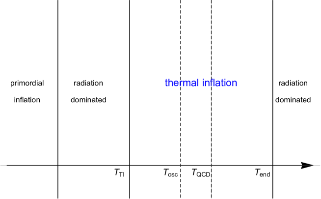
Figure 1: Thermal history of (QCD) axion scenario with thermal inflation. The horizontal axis represents the direction of time evolution. Here, different boundaries are labeled by the temperatures of background radiation.

In any case, even when the energy transfer occurs instantaneously, the total energy density $\rho$ and the spacetime metric, especially, the scale factor $a=\exp(\bar{N}+\psi)$ must be continuous. On the other hand, each component of the energy density $\rho_{X}$ can be discontinuous and consequently $\zeta_{X}$ has discontinuity. The curvature perturbation $\zeta=-\psi+\delta\rho/3(\rho+P)$ is also discontinuous unless $\delta\rho=0$ since the EOS and accordingly the pressure $P$ is discontinuous between adjacent phases.

$\bullet$ Axion perturbations and amplitude of CMB
PQ symmetry of the axion field $A$ is assumed to be already broken before the primordial inflation. Then axion field fluctuations $\delta A\neq 0$ are generated during the primordial inflation. In a very high temperature universe, axion does not have potential and its energy density is negligible. Suppose that axion potential is suddenly generated when temperature drops down to $T_{A}$. Then axion energy density increases by transferring energy from radiation. By an appropriate gauge transformation, we can take a constant time slice on which this sudden transition takes place. In absence of any other components to fluctuate, this is a uniform density slice $\delta\rho=0$, and thus we have $\psi=-\zeta_{\rm inf}$ where $\zeta_{\rm inf}$ is the curvature perturbation originated from inflaton’s perturbation. Before the transition, the density fluctuation is equal to the temperature fluctuation and the slice is characterized by $T=T_{A}$. In the following, we generally call this slice “QCD slice”. After the transition, on the other hand, radiation energy is transferred to the axion field which has inhomogeneous primordial fluctuations, and the slice is no longer a uniform temperature slice. Indeed, from the energy conservation right after the transition, we have $\delta\rho_{r}=-\delta\rho_{A}\neq 0$ whose sum vanishes

$$\delta\rho=\delta\rho_{r}+\delta\rho_{A}=0~{},$$ (25)

or equivalently, using Eq. (8),

$$\Omega_{r}\left[e^{{-4(\zeta_{r}-\zeta_{\rm inf})}}-1\right]+\frac{\rho_{A}-\bar{\rho}_{A}}{\bar{\rho}}=0.$$ (26)

Solving this equation with respect to $\zeta_{r}$, we obtain

$$\zeta_{r}=\zeta_{\rm inf}-\frac{1}{4}\ln\left(1-R\frac{\rho_{A}-\bar{\rho}_{A}}{\bar{\rho}_{A}}\right)~{}$$ (27)

where

$$R:=\frac{\Omega_{A}}{\Omega_{r}}\bigg{|}_{\rm right~{}after~{}transition}$$ (28)

is the ratio of the energy densities of axion to radiation evaluated right after the sudden potential generation at $T=T_{A}$.

Axion energy density is given by the axion potential $\rho_{A}\simeq V_{A}(\bar{A})$ either for a slow-rolling case ($\bar{A}$ is the field value) or for an oscillating case ($\bar{A}$ is the amplitude of the oscillation). In our situation, we assume that $\zeta_{\rm inf}$ is too small to explain the CMB anisotropy and focus on the axion fluctuations as its origin. In the following we set $\zeta_{\rm inf}=0$. At the linear order in the fluctuation of $\delta A_{\rm ini}$, $\zeta_{r}$ in Eq. (27) becomes

$$\zeta_{r{\rm G}}=\frac{R}{4}\left.\frac{V_{A}^{{}^{\prime}}}{V_{A}}\right|_{A=\bar{A}_{\rm QCD}}\times\left(\frac{\delta A_{\rm QCD}}{\delta A_{\rm ini}}\right)\delta A_{\rm ini}={\cal X}(\bar{\theta}_{\rm QCD})~{}{\cal Y}(\bar{\theta}_{\rm QCD})~{}\frac{R}{2}\frac{\delta A_{\rm ini}}{\bar{A}_{\rm ini}}~{},$$ (29)

where we rewrote the fluctuation $\delta A_{\rm QCD}$ at $T_{\rm QCD}$ in terms of the initial Gaussian fluctuation $\delta A_{\rm ini}$ created during the primordial inflation. $\theta=A/f_{A}$ is the dimensionless angle of the axion field. We also defined anharmonicity factors ${\cal X}(\bar{\theta}_{\rm QCD})$ and ${\cal Y}(\bar{\theta}_{\rm QCD})$ by

$${\cal X}(\bar{\theta}_{\rm QCD}):=\frac{1}{2}\left.\frac{\partial\ln V_{A}}{\partial\ln A}\right|_{A=\bar{A}_{\rm QCD}}=\frac{\bar{\theta}_{\rm QCD}\sin(\bar{\theta}_{\rm QCD})}{2(1-\cos(\bar{\theta}_{\rm QCD}))}=\frac{\bar{\theta}_{\rm QCD}}{2\tan(\bar{\theta}_{\rm QCD}/2)}~{},$$ (30)

$${\cal Y}(\bar{\theta}_{\rm QCD}):=\frac{\bar{\theta}_{\rm ini}}{\bar{\theta}_{\rm QCD}}\overline{\frac{\delta\theta_{\rm QCD}}{\delta\theta_{\rm ini}}}~{},$$ (31)

${\cal X}$ is the anharmonicity factor associated with the anharmonicity of the potential $V_{A}(A)$, and we have used the explicit sinusoidal form of the potential $V_{A}\propto 1-\cos\theta$ in Eq. (50). In the harmonic limit with $\theta\ll 1$ it goes to unity. The factor ${\cal Y}$ takes into account axion’s evolution before the QCD slice. The overline denotes that $\theta$ is replaced by the spatially homogeneous angle $\bar{\theta}$. It is almost unity for the scenarios we work on in the next section; either axion’s evolution is almost linear or the axion field does not evolve so much before the QCD slice, see Eq. (68). The subscript G of $\zeta_{r{\rm G}}$ stands for the fact that axion’s fluctuations created during the primordial inflation is Gaussian, and they have the almost scale invariant spectrum,

$$\langle\delta A_{{\rm ini}}(k)\delta A_{{\rm ini}}(k^{\prime})\rangle=(2\pi)^{3}\delta^{(3)}(k+k^{\prime})\frac{\overline{H}^{2}_{\rm exit}(k)}{2k^{3}}~{},~{}~{}~{}~{}\overline{H}_{\text{exit}}(k):=\overline{H}|_{k=a\overline{H}}~{}.$$ (32)

Generally speaking, the above curvature perturbation $\zeta_{r}$ is not yet the final CMB fluctuation we observe today because further mixings with other fields after the transition $T=T_{A}$ may contribute to the curvature perturbation. If there are no such mixings and the energy density of radiation is taken over to the current density of radiation, this gives the final CMB fluctuations. In thermal inflation scenario discussed in next section, as well as in the standard QCD scenario, the fluctuation Eq. (29) is almost copied to the fluctuation of radiation, i.e. CMB anisotropy. See Appendix C for more details. Therefore, from Eq. (29), the scalar spectrum amplitude of CMB is given by

$$\sqrt{A_{s}}=R\times\frac{\overline{H}_{\text{exit}}(k_{*})}{4\pi f_{A}\overline{\theta}_{\rm ini}}{\cal X}(\bar{\theta}_{\rm QCD}){\cal Y}(\bar{\theta}_{\rm QCD})~{}.$$ (33)

Comparing it with the CMB observation in Eq. (19), this gives a relation between $R$ and $\overline{H}_{\text{exit}}(k_{*})/\pi f_{A}$ for each misalignment angle $\bar{\theta}_{\rm QCD}$.

$\bullet$ Non-Gaussianity
We then calculate the non-Gaussianity. With the assumption $\zeta_{\rm inf}=0$ and $\rho_{A}\simeq V_{A}(A)$, the nonlinear expression Eq. (27) is expanded with respect to $\delta A_{\rm QCD}$ as

$$\zeta_{r} =\frac{R}{4}\left.\frac{\bar{V}_{A}^{{}^{\prime}}}{\bar{V}_{A}}\right|_{\rm QCD}\delta A_{\rm QCD}+\frac{R}{8}\left[\frac{\bar{V}_{A}^{{}^{\prime\prime}}}{\bar{V}_{A}}+R\left(\frac{\bar{V}_{A}^{\prime}}{\bar{V}_{A}}\right)^{2}\right]_{\rm QCD}(\delta A_{\rm QCD})^{2}$$

$$~{}~{}~{}~{}~{}~{}~{}~{}~{}~{}~{}~{}~{}~{}~{}~{}~{}+\frac{R}{12}\left[\frac{\bar{V}_{A}^{{}^{\prime\prime\prime}}}{2\bar{V}_{A}}+\frac{3R}{2}\frac{\bar{V}_{A}^{{}^{\prime}}\bar{V}_{A}^{{}^{\prime\prime}}}{\bar{V}_{A}^{2}}+R^{2}\left(\frac{\bar{V}_{A}^{\prime}}{\bar{V}_{A}}\right)^{3}\right]_{\rm QCD}(\delta A_{\rm QCD})^{3}+\cdots$$ (34)

$$=\zeta_{r{\rm G}}+\frac{2}{R}\left[\frac{\bar{V}_{A}^{{}^{\prime\prime}}\bar{V}_{A}}{\bar{V}_{A}^{{}^{\prime}2}}+R\right]_{\rm QCD}\zeta_{r{\rm G}}^{2}+\frac{16}{3R^{2}}\left[\frac{\bar{V}_{A}^{{}^{\prime\prime\prime}}\bar{V}_{A}^{2}}{2\bar{V}_{A}^{{}^{\prime}3}}+\frac{3R}{2}\frac{\bar{V}_{A}^{{}^{\prime\prime}}\bar{V}_{A}}{\bar{V}_{A}^{{}^{\prime}2}}+R^{2}\right]_{\rm QCD}\zeta_{r{\rm G}}^{3}+\cdots~{}.$$

In the last line, $A_{\rm QCD}=A_{\rm ini}$ is assumed for brevity, so that ${\cal Y}=1$. The anharmonicity factor ${\cal Y}$ gives a small correction to the non-Gaussianity, which we discuss later in Eqs. (71)(72). From this, we obtain

$$f_{\rm NL} =-\frac{10}{3R}\left[\frac{\bar{V}_{A}^{{}^{\prime\prime}}\bar{V}_{A}}{\bar{V}_{A}^{{}^{\prime}2}}+R\right]_{\rm QCD}~{},$$ (35)

$$g_{\rm NL} =\frac{1}{3}\left(\frac{20}{3R}\right)^{2}\left[\frac{\bar{V}_{A}^{{}^{\prime\prime\prime}}\bar{V}_{A}^{2}}{2\bar{V}_{A}^{{}^{\prime}3}}+\frac{3R}{2}\frac{\bar{V}_{A}^{{}^{\prime\prime}}\bar{V}_{A}}{\bar{V}_{A}^{{}^{\prime}2}}+R^{2}\right]_{\rm QCD}$$ (36)

$$=\frac{1}{6}\left(\frac{20}{3R}\right)^{2}\left.\frac{\bar{V}_{A}^{{}^{\prime\prime\prime}}\bar{V}_{A}^{2}}{\bar{V}_{A}^{{}^{\prime}3}}\right|_{\rm QCD}+\frac{20}{3}f_{\rm NL}-\frac{1}{6}\left(\frac{20}{3}\right)^{2}.$$

In the case of the sinusoidal potential $V_{A}(\overline{\theta})\propto 1-\cos\overline{\theta}$, we have

$$f_{\rm NL}=-\frac{10}{3R}\frac{\cos(\overline{\theta}_{\rm QCD})\left(1-\cos(\overline{\theta}_{\rm QCD})\right)}{\sin^{2}(\overline{\theta}_{\rm QCD})}-\frac{10}{3}~{},$$ (37)

$$g_{\rm NL}=-\frac{1}{6}\left(\frac{20}{3R}\right)^{2}\tan^{2}\left(\frac{\overline{\theta}_{\rm QCD}}{2}\right)+\frac{20}{3}f_{\rm NL}-\frac{1}{6}\left(\frac{20}{3}\right)^{2}.$$ (38)

Note that the non-Gaussianities are inversely proportional to $R$ since the leading Gaussian fluctuation is proportional to $R\ (<1)$ while the leading non-linear terms also proportional to $R$ instead of decreasing with higher orders of $R$.

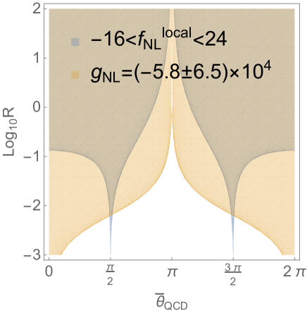
Figure 2: Allowed regions of $(\overline{\theta}_{\rm QCD},R)$ by the non-Gaussianity constraints, Eq.(24). The blue (orange) region represents the region allowed by $f_{\rm NL}\ (g_{\rm NL})$. $\overline{\theta}\sim\pi/2,3\pi/2$ is necessary to obtain $R\sim{\cal{O}}(0.01)$, where $V^{\prime\prime}$ vanishes.

In Fig.2, we plot the allowed region of $(\overline{\theta}_{\rm QCD},R)$ determined by the observational constraints in Eq. (24). The blue (orange) region corresponds to $f_{\rm NL}\ (g_{\rm NL})$. One can see that, as long as $\overline{\theta}_{\rm QCD}\sim 0$, the lower bound of $R$ is ${\cal{O}}(0.1)$, but as $\overline{\theta}_{\rm QCD}$ approaches $\pi/2$ or $3\pi/2$, the bound can be reduced to $\ {\cal{O}}(0.01)$ because $V_{A}^{{}^{\prime\prime}}$ vanishes at these points. It is interesting that around these values of $\overline{\theta}_{\rm QCD}$, $g_{\rm NL}$ becomes sizable while reducing $f_{\rm NL}$.

$\bullet$ Isocurvature perturbations
As discussed in section 2.2, the magnitude of the isocurvature perturbation is measured by ${\cal{I}}=r_{A}S_{A}$, where $S_{A}$ is given by Eq.(12). At sufficiently late time (after the QCD transition but before the last scattering), the axion field $A(t)$ becomes very small and we can approximate its potential by the harmonic one , $V_{A}(A)=m_{A0}^{2}A^{2}/2$, and hence, the EOS is given by $w_{A}=0$. By denoting such time slice as late time, and choosing an uniform temperature slice of $\zeta_{r}=-\psi$, $S_{A}$ can be simply evaluated to linear order in $\delta\theta$ as

$$S_{A}=\ln\left.\frac{V_{A}(A)}{V_{A}(\bar{A})}\right|_{\rm late\ time}\simeq 2\left.\frac{\delta\theta}{\bar{\theta}}\right|_{\rm late\ time}~{},$$ (39)

where we used the expression Eq. (8) in the first equality. In order to relate the fluctuation at late time with the initial one of Eq. (32), we need to solve the evolution of the axion field from the horizon exit until the late time slice. To quantify the power spectrum of the isocurvature fluctuation, we introduce

$${\cal Z}(\bar{\theta}_{\rm QCD}):=\frac{\bar{\theta}_{\rm QCD}}{\bar{\theta}|_{\rm late\ time}}\frac{\delta\theta|_{\rm late\ time}}{\delta\theta_{\rm QCD}}~{}.$$ (40)

The quantity ${\cal Z}$ depends on how much energy is transferred from radiation to axion at the QCD slice and also on the anharmonicity of the potential in which the axion evolves after the QCD slice. The former effect turns out to be subdominant since $R\ll 1$. Indeed, as we will see in next section, the conventional QCD-axion scenario with the almost harmonic potential gives ${\cal Z}\simeq 1+3R/4$. On the other hand, the thermal inflation model with QCD-axion gives ${\cal Z}\simeq\bar{\theta}_{\rm QCD}/\sin(\bar{\theta}_{\rm QCD})+{\cal O}(R)>1$ since axion field rolls down in the anharmonic region of the potential during thermal inflation, see Eq. (80).

Now the isocurvature power spectrum is given as

$${\cal{P}}_{{\cal II}}(k)=\frac{k^{3}}{2\pi^{2}}P_{{\cal{I}}}(k)=\left({\cal Y}(\bar{\theta}_{\rm QCD}){\cal Z}(\bar{\theta}_{\rm QCD})~{}\frac{r_{A}\overline{H}_{\rm exit}(k)}{\pi f_{A}\overline{\theta}_{\rm ini}}\right)^{2}~{}.$$ (41)

Note that ${\cal Y}{\cal Z}=(\bar{\theta}_{\rm ini}/\bar{\theta}|_{\rm late\ time})(\delta\theta|_{\rm late\ time}/\delta\theta_{\rm ini})$ gives an anharmonicity factor associated with the evolution of the axion field from the initial slice to the late time. By plugging this into Eq. (23) and using ${\cal{P}}_{{\cal RR}}(k_{*})=2.1\times 10^{-9}$, we obtain the following constraint

$${\cal Y}(\bar{\theta}_{\rm QCD}){\cal Z}(\bar{\theta}_{\rm QCD})~{}\frac{r_{A}\overline{H}_{\rm exit}(k_{*})}{\pi f_{A}\overline{\theta}_{\rm ini}}<1.5\times 10^{-6}\quad\text{ for }\cos\Delta=-1\ .$$ (42)

This bound gives a strong constraint on $r_{A}$ and $\overline{H}_{\text{exit}}(k)/f_{A}$.

3.2 Allowed parameter region

In the previous section, without specifying models, we calculated the (iso-)curvature perturbations and their non-Gaussianity under an assumption that primordial fluctuations of QCD-axion like particles generate the CMB anisotropy. The results are summarized as follows:

• Amplitude of scalar power spectrum Eq. (33) is given by

  $$\sqrt{A_{s}}=R{\cal X}(\overline{\theta}_{\rm QCD}){\cal Y}(\overline{\theta}_{\rm QCD})\frac{\overline{H}_{\text{exit}}(k_{*})}{4\pi f_{A}\overline{\theta}_{\rm ini}}=4.6\times 10^{-5}$$ (43)

• Isocurvature constraint of Eq. (42) must be satisfied,

  $${\cal Y}(\overline{\theta}_{\rm QCD}){\cal Z}(\overline{\theta}_{\rm QCD})~{}\frac{r_{A}\overline{H}_{\rm exit}(k_{*})}{\pi f_{A}\overline{\theta}_{\rm ini}}<1.5\times 10^{-6}$$ (44)

• Non-Gaussianity constraints of $f_{\rm NL}$ and $g_{\rm NL}$ in Fig.2 must be satisfied. For most values of $\bar{\theta}_{\rm QCD}$, the ratio $R$ must satisfy the condition, $R\gtrsim 0.1$. If $\bar{\theta}_{\rm QCD}$ is tuned around special values, the constraint is weakened to

  $$R\gtrsim 0.01\quad\left(\text{around}\ \bar{\theta}_{\rm QCD}=\pi/2\ \text{or}\ 3\pi/2\right).$$ (45)

These relations (43), (44) and (45) are plotted in Fig.3. Here, we put ${\cal X}={\cal Y}={\cal Z}=1$ for simplicity.

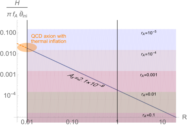
Figure 3: The parameters must be on the blue line on which the correct scalar amplitude Eq. (43) is produced. In each colored region, the maximum value of $r_{A}$ is indicated which is determined by Eq. (44). Thermal inflation scenario discussed in the next section typically lies on the orange region.

From Eq. (45) and Eq. (43), we have a condition for the Hubble parameter of the primordial inflation as

$${\cal X}(\overline{\theta}_{\rm QCD}){\cal Y}(\overline{\theta}_{\rm QCD})\frac{\overline{H}_{\text{exit}}(k_{*})}{4\pi f_{A}\overline{\theta}_{\rm ini}}<4.6\times 10^{-3}.$$ (46)

Further, by eliminating $\overline{H}_{\text{exit}}(k_{*})/(f_{A}\overline{\theta}_{\rm ini})$ from Eqs. (43) and (44), we obtain an inequality between $r_{A}$ and $R$ as

$$r_{A}<8.2\times 10^{-3}\ R\frac{{\cal X}(\overline{\theta}_{\rm QCD})}{{\cal Z}(\overline{\theta}_{\rm QCD})}~{}.$$ (47)

This shows that $r_{A}\ll 1$ and axions cannot dominate the dark matter in the current scenario. If the universe is radiation dominated right after the transition, we have $R\simeq\Omega_{A}|_{T=T_{A}}$. Neglecting the anhamonicity and nonlinearity factors, $r_{A}\lesssim 8.2\times 10^{-3}\Omega_{A}|_{T=T_{A}}\ll 8.2\times 10^{-3}$ is obtained. As we see in next section, this rules out the standard QCD axion to explain the CMB anisotropy.

Finally, we should emphasize that the current axion scenario can predict a large value of $|g_{\rm NL}|\sim 10^{4}$ when $R\sim 0.01$ and $\bar{\theta}_{\rm QCD}\simeq\pi/2,3\pi/2$. Such a parameter region is interesting since the scenario can be testable in the future cosmological observations of $g_{\rm NL}$. As we will see below, a thermal inflation model with the QCD axion can be in this parameter region.

4 Models

Now we investigate a few particle physics models of the axion scenario for the CMB anisotropy. In section 4.1, we first briefly summarize why the standard QCD axion in the standard thermal history of the universe cannot satisfy the conditions; main difficulty is to satisfy the inequality Eq. (47) since axions cannot be sufficiently diluted after the QCD transition. Thus we need an additional mechanism to dilute the axion abundance. For this purpose, we consider a thermal inflation scenario in the next section 4.2. Suppose that the temperature of the universe decreases below the QCD temperature during the thermal inflation as depicted in Figure 1, one may suspect that axions are diluted even before $T_{\rm QCD}$ and $R$ becomes too small. We will see, however, that since the Hubble of the thermal inflation is larger than the axion mass, $3H_{\rm TI}\gtrsim m_{A}(T)$, the axion field does not evolve so much before $T_{\rm QCD}$. As a result, we can realize $R\sim 0.01$ simultaneously with a small $r_{A}$ provided that the thermal inflation lasts long enough below $T_{\rm QCD}$. We investigate parameter regions in which the above conditions are satisfied and the axion field fluctuations can explain the CMB anisotropy. As a particle physics model to realize a thermal inflation, we briefly comment on a classically conformal $B$-$L$ model with a QCD axion [61, 62, 63, 64] in the final section. A novel feature of the model is that the universe has experienced supercooling era of the $B$-$L$ and EW symmetries, and thermal inflation occurs at around TeV scale and continues down to QCD temperature. However, as shown in [64], this model predicts a small Higgs vacuum expectation value of the QCD scale, $\langle h\rangle|_{T_{\rm QCD}}\sim\Lambda_{\rm QCD}$ when the axion potential is generated, and the height of the axion potential becomes too small for getting a sufficiently large value of $R$. Thus we need some modifications of the original classically conformal $B$-$L$ model, such as including a Higgs-axion mixing.

4.1 No-go for the standard QCD axion

We recap the calculations in the standard QCD axion scenario to recall the difficulty of realizing the large-scale fluctuations. Below the QCD temperature $T_{\rm QCD}\simeq 150{\rm MeV}$, the axion potential is given by

$$V_{A0}=m_{A0}^{2}f_{A}^{2}[1-\cos(A/f_{A})]~{},$$ (48)

$$m_{A0}=\frac{\sqrt{m_{u}/m_{d}}}{1+m_{u}/m_{d}}\frac{m_{\pi}f_{\pi}}{f_{A}}\simeq 6\times 10^{-6}{\rm eV}\times\frac{10^{12}{\rm GeV}}{f_{A}}$$ (49)

with $m_{u}/m_{d}\simeq 0.48$, $m_{\pi}\simeq 135{\rm MeV}$ and $f_{\pi}\simeq 93{\rm MeV}$. For $T\geq T_{\rm QCD}$, it has a strong temperature dependence

$$V_{A}=m_{A}(T)^{2}f_{A}^{2}[1-\cos(A/f_{A})]\ \text{ where }\ m_{A}(T)=m_{A0}[T_{\rm QCD}/T]^{4b}~{}.$$ (50)

The exponent is given by $b\simeq 1.02$ in the case of three light quarks [65]. The axion acquires tiny but finite potential energy once the EW symmetry is broken at $T=T_{\rm EW}\sim 160{\rm GeV}$. In this work, we do not take into account the temperature dependence of the number of dynamical quarks and simply assume that $b$ is constant for $T_{\rm EW}\geq T\geq T_{\rm QCD}$.

$\bullet$ Estimation of $R$ and scalar amplitude
We assume for simplicity that, the axion field value is sufficiently small and anharmonicity of the potential can be neglected, $V_{A}\simeq m_{A}^{2}A^{2}/2$. When the condition $m_{A}\geq 3\overline{H}$ is satisfies, axion field starts oscillating. If the oscillation occurs before $T_{\rm QCD}$, the oscillation temperature is given by

$$T_{\rm osc} = T_{\rm QCD}\times\left[\sqrt{\frac{10}{\pi^{2}g_{\rm osc}}}\frac{m_{A0}m_{Pl}}{T_{\rm QCD}^{2}}\right]^{\frac{1}{4b+2}}$$

$$\simeq {\rm GeV}\times\left(\frac{T_{\rm QCD}}{150{\rm MeV}}\right)^{0.67}\left(\frac{10^{12}{\rm GeV}}{f_{A}}\right)^{0.16}.\$$

Here we used the effective number of degrees of freedom $g_{\rm osc}=62$ at $T\sim{\rm GeV}$ [67] and $b\simeq 1.02$. Below $T_{\rm osc}$, the evolution of the axion field is almost adiabatic and axion’s “number density” is given by

$$\bar{n}_{A}=\bar{n}_{A}|_{\rm osc}\times(\bar{a}_{\rm osc}/\bar{a})^{3}~{}~{}~{},~{}~{}~{}~{}n_{A}|_{\rm osc}=\left.\frac{\bar{\rho}_{A}}{m_{A}}\right|_{\rm osc}~{}.$$ (52)

Then the temperature dependence of the energy density is evaluated as

$$\bar{\rho}_{A} = m_{A}\times\bar{n}_{A}=\left(\frac{T_{\rm QCD}}{T}\right)^{4b-3}\left(\frac{T_{\rm QCD}}{T_{\rm osc}}\right)^{4b+3}V_{A0}(\bar{A}_{\rm osc})~{}.$$ (53)

On the other hand, the ratio of the energy densities at $T=T_{\rm QCD}$ is given by

$$R = \frac{\bar{\rho}_{A}}{\bar{\rho}_{r}}\bigg{|}_{T=T_{\rm QCD}}=\frac{m_{u}/m_{d}}{(1+m_{u}/m_{d})^{2}}\frac{m_{\pi}^{2}f_{\pi}^{2}}{T_{\rm QCD}^{4}}\frac{30}{\pi^{2}g_{\rm QCD}}\left(\frac{T_{\rm QCD}}{T_{\rm osc}}\right)^{4b+3}\frac{\bar{\theta}^{2}_{\rm osc}}{2}$$ (54)

$$\simeq 1.2\times 10^{-8}\left(\frac{f_{A}}{10^{12}{\rm GeV}}\right)^{1.16}\left(\frac{150{\rm MeV}}{T_{\rm QCD}}\right)^{1.67}\bar{\theta}^{2}_{\rm osc},$$

where we used $g_{\rm QCD}=69/4$ as the effective number of degrees of freedom right after the QCD phase transition to which pions also contribute. The axion angle $\overline{\theta}_{\rm osc}$ can be identified with $\overline{\theta}=\overline{\theta}_{\rm ini}$ because the amplitude does not change during this period. The small numerical coefficient mainly comes from the damping of the oscillation amplitude, $(\bar{\theta}_{\rm QCD}/\bar{\theta}_{\rm osc})^{2}\simeq(T_{\rm QCD}/T_{\rm osc})^{4b+3}\sim 10^{-6}$. The smallness of $R$ already rejects the scenario, but let us go on for comparison with thermal inflation models discussed in the next section. We plug the result into Eq. (33) together with the approximations, ${\cal X}=1$ (harmonic approximation) and ${\cal Y}=1$. Then, using the observational value of the CMB anisotropy, $A_{s}\simeq 2.1\times 10^{-9}$, we have the condition

$$\overline{\theta}_{\rm ini}\times\frac{\overline{H}_{\text{exit}}(k_{*})}{\pi f_{A}}\simeq 1.6\times 10^{4}\left(\frac{10^{12}{\rm GeV}}{f_{A}}\right)^{1.16}\left(\frac{T_{\rm QCD}}{150{\rm MeV}}\right)^{1.67}.$$ (55)

$\bullet$ Isocurvature fluctuations
Now, let us evaluate the amplitude of the isocurvature fluctuation. The time slice of axion’s potential generation is no longer a uniform temperature slice after the QCD transition. Consequently, the ratio $\delta A/\bar{A}$ evaluated on a uniform temperature slice after the transition is different from the one evaluated on a uniform temperature slice before the transition. This effect is taken into account by a factor ${\cal Z}=1+3R/4$ which is practically irrelevant due to the smallness of $R$. Noting that $R$ can be also rewritten in terms of the present axion abundance $r_{A}$ as

$$R =\frac{\rho_{A}}{\rho_{\gamma}}\bigg{|}_{\rm today}\frac{(a_{\rm today}/a_{\rm QCD})^{3}}{(T_{\rm QCD}/T_{0})^{3}g_{\rm QCD}/g_{\gamma}}$$

$$=r_{A}\left.\frac{\Omega_{\rm CDM}}{\Omega_{\gamma}}\right|_{\rm today}\frac{T_{0}}{T_{\rm QCD}}\simeq 8\times 10^{-9}\times\ r_{A}\left(\frac{150{\rm MeV}}{T_{\rm QCD}}\right)$$ (56)

where $T_{0}\simeq 2.35\times 10^{-4}$eV is the CMB temperature, the CDM and photon energy density fractions today are $\Omega_{\rm CDM}\simeq 2.65\times 10^{-1}$ and $\Omega_{\gamma}\simeq 5.38\times 10^{-5}$, respectively. Using Eq. (54), the ratio $r_{A}$ and the misalignment angle $\bar{\theta}_{\rm ini}$ are related as

$$r_{A}\simeq 1.5\times\left(\frac{150{\rm MeV}}{T_{\rm QCD}}\right)^{0.67}\left(\frac{f_{A}}{10^{12}{\rm GeV}}\right)^{1.16}\bar{\theta}_{\rm ini}^{2}~{}.$$ (57)

Then the condition (44) for the isocurvature constraint becomes

$$\overline{\theta}_{\rm ini}\ \frac{\overline{H}_{\text{exit}}(k_{*})}{\pi f_{A}}<10^{-6}\left(\frac{10^{12}{\rm GeV}}{f_{A}}\right)^{1.16}\left(\frac{T_{\rm QCD}}{150{\rm MeV}}\right)^{0.67},$$ (58)

which conflicts with Eq. (55). In another word, the inequality Eq. (47) does not hold.

In this standard scenario, there are essentially two difficulties to realize the scenario of QCD axion as the source of the CMB anisotropy. One difficulty is absence of sufficient dilution after the axion potential is produced until present, necessary to suppress the large isocurvature fluctuations. In addition, since the axion potential is generated at higher temperature than $T_{\rm QCD}$, the amplitude of the axion oscillation damps before the efficient energy transfer between radiation and axion at the QCD transition. Combined with the smallness of the axion potential at $T=T_{\rm osc}$, these effects result in too small $R$, and it is difficult to reproduce the sufficient amount of the scalar amplitude. It also contradicts with the non-Gaussianity constraint. In the next section, we consider thermal inflation scenario in which both of the difficulties can be evaded.

4.2 QCD axion with thermal inflation

One of possibilities to realize the dilution of the QCD axion field is thermal inflation [40, 41, 42, 43] that lasts until below the QCD phase transition. The scalar field whose potential energy drives this short inflation is often dubbed “flaton” and trapped at a symmetry-enhancing point due to the thermal effect. Precise cosmological predictions are model-dependent. Our purpose here is to give a general quantitative argument of the QCD axion scenario which undergoes the thermal inflation. In addition to the existence of a QCD axion, we assume the following situations:

• Thermal inflation starts at temperature $T_{\rm TI}\gg T_{\rm QCD}$.

• Thermal inflation ends at a low temperate $T_{\rm end}\ll T_{\rm QCD}$, and then reheating occurs by decay of flaton into the SM particles.

• The reheating temperature is higher than the oscillation temperature $T_{\rm osc}$. Subsequently, the standard Big Bang thermal history with the axion field follows as discussed in the previous section.

• Flaton sector does not have interactions with the QCD axion.

The last two are assumed for simplicity. The temperature fluctuation $\zeta_{r}$ generated at $T=T_{\rm QCD}$ during the thermal inflation causes the fluctuation of e-foldings between the QCD slice and the “end” slice at $T=T_{\rm end}$ (see Eq. (79) below), and hence, the CMB anisotropy that we observe today. One can also track the fluctuation being transferred to flaton’s oscillation and then to the final radiation component, as discussed in Appendix C.

The thermal inflation starts when the vacuum energy dominates. Provided that the radiation is dominant before the thermal inflation, the temperature $T_{\rm TI}$ at its onset is evaluated by $V_{\rm TI}=(g_{\rm TI}\pi^{2}/30)T_{\rm TI}^{4}$ where $g_{\rm TI}$ is the degrees of freedom at $T=T_{\rm TI}$. Once the thermal inflation starts, the radiation is quickly diluted so that the Hubble expansion rate is well approximated by the constant

$$H_{\rm TI}^{2}=\frac{V_{\rm TI}}{3m_{Pl}^{2}}=(1.4\times 10^{-3}{\rm eV})^{2}\left(\frac{g_{\rm TI}}{100}\right)\left(\frac{T_{\rm TI}}{1{\rm TeV}}\right)^{4}~{}.$$ (59)

In the following, we treat $T_{\rm TI}$, $T_{\rm end}$ and the decay constant of axion $f_{A}$ as free parameters.

$\bullet$ Estimation of $R$ and amplitude of CMB
If the axion potential is generated during the thermal inflation with the Hubble $H_{\rm TI}$, the axion field does not oscillate to get diluted before the QCD transition, unlike the standard QCD axion discussed in the previous section. In order to estimate the value of $R$, we first solve the equation of motion (EOM) of the QCD axion field $(-g)^{-1/2}\partial_{\mu}\left\{(-g)^{1/2}g^{\mu\nu}\partial_{\nu}A\right\}=\partial_{A}V_{A}$ for $T\geq T_{\rm QCD}$ where the potential has the strong temperature dependence Eq. (50). In order to avoid dilution of axion’s energy density, we focus on the parameter region where the axion field obeys a slow-roll attractor equation

$$3\alpha H\dot{A}/\lambda+\partial_{A}V_{A}=0$$ (60)

with a numerical parameter $\alpha$. Plugging this into axion’s EOM [68, 69, 66] and approximating the Hubble expansion rate by the constant $H_{\rm TI}$, we get the condition for the attractor equation to be valid;

$$\frac{\partial_{A}^{2}V_{A}}{3\alpha H_{\rm TI}^{2}}=\frac{\eta}{\alpha}\times\left(\frac{T_{\rm QCD}}{T}\right)^{8b}\cos(\theta)\ll 1$$ (61)

where $\alpha=1+8b/3\simeq 3.7$ and $\eta$ is given by

$$\eta:=\frac{1}{3}\left(\frac{m_{A0}}{H_{\rm TI}}\right)^{2}=6.6\times 10^{-6}\left(\frac{100}{g_{\rm TI}}\right)\left(\frac{10^{12}{\rm GeV}}{f_{A}}\right)^{2}\left(\frac{1{\rm TeV}}{T_{\rm TI}}\right)^{4}~{}.$$ (62)

The above inequality is satisfied all the way down to $T=T_{\rm QCD}$ regardless of the field value $\theta=A/f_{A}$ as far as the inequality $\eta\ll\alpha$ is satisfied. Let us define the following evolution parameter $\Delta(t)$ by

$$\Delta(t):=H_{\rm TI}\int_{t_{\rm QCD}}^{t}\lambda dt\leq 0$$ (63)

in the constant $H_{\rm TI}$. Note that it takes a negative value since we are interested in the evolution for $t<t_{\rm QCD}$; thus it is a minus e-folding number. Neglecting an effect of gradual energy transfer from radiation to axion as in the previous section, we have $T/T_{\rm QCD}=e^{-\Delta}$ for $T<T_{\rm EW}$. Then, the attractor equation, Eq.(60), is written as

$$\frac{d\theta}{d\Delta}=-\frac{\eta}{\alpha}e^{8b\Delta}\sin\theta~{}.$$ (64)

Assuming $T_{\rm TI}>T_{\rm EW}$ and integrating $\Delta$ from $\Delta_{\rm EW}:=\ln T_{\rm QCD}/T_{\rm EW}\ll-1$ to $0$, we obtain

$$\ln\frac{\tan\left(\theta_{\rm QCD}/2\right)}{\tan\left(\theta_{\rm ini}/2\right)}=-\frac{\eta}{8b\alpha}\left(1-e^{8b\Delta_{\rm EW}}\right)\simeq-\frac{\eta}{8b\alpha}~{},$$ (65)

where we have plugged $\theta|_{T=T_{\rm EW}}=\theta_{\rm ini}$ and used $e^{8b\Delta_{\rm EW}}\ll 1$. We can see that, because of the strong temperature dependence of the potential $\propto T^{-8b}$, the integration is dominated by the contribution around the upper limit $\Delta=0$. This is also the case for $T_{\rm TI}<T_{\rm EW}$ as far as $T_{\rm TI}\gg T_{\rm QCD}$. Hence, we obtain

$$\theta_{\rm ini}=2\arctan\left\{e^{\frac{\eta}{8b\alpha}}\tan\left(\theta_{\rm QCD}/2\right)\right\}=\theta_{\rm QCD}+y\sin(\theta_{\rm QCD})+{\cal O}\left(y^{2}\right)~{}.$$ (66)

On the last equality, the dependence on $y:=\eta/8b\alpha\ll 1$ is expanded. By differentiating it with respect to $\theta_{\rm QCD}$, we get

$$\frac{\delta\theta_{\rm ini}}{\delta\theta_{\rm QCD}}=\frac{1}{\cosh(y)-\sinh(y)\cos(\theta_{\rm QCD})}=1+y\cos(\theta_{\rm QCD})+{\cal O}\left(y^{2}\right)~{}.$$ (67)

Therefore, the quantity $\cal Y$ in Eq. (29) is computed as

$${\cal Y}(\bar{\theta}_{\rm QCD})=\left.\left(\frac{\bar{\theta}_{\rm ini}}{\bar{\theta}_{\rm QCD}}\right)\middle/\ \overline{\left(\frac{\delta\theta_{\rm ini}}{\delta\theta_{\rm QCD}}\right)}\right.=1+y\left(\frac{\sin(\bar{\theta}_{\rm QCD})}{\bar{\theta}_{\rm QCD}}-\cos(\bar{\theta}_{\rm QCD})\right)+{\cal O}(y^{2})~{}.$$ (68)

These results show that the axion field does not evolve much until $T=T_{\rm QCD}$.

In terms of the averaged angle $\overline{\theta}_{\rm QCD}$ at the QCD scale, the ratio of the energy densities is given by

$$R =\frac{\rho_{A}}{\rho_{r}}\bigg{|}_{T=T_{\rm QCD}}\simeq\frac{30}{\pi^{2}g_{\rm QCD}}\frac{m_{u}/m_{d}}{(1+m_{u}/m_{d})^{2}}\frac{m_{\pi}^{2}f_{\pi}^{2}}{T_{\rm QCD}^{4}}(1-\cos(\overline{\theta}_{\rm QCD}))$$

$$\simeq 0.012\times\left(\frac{150{\rm MeV}}{T_{\rm QCD}}\right)^{4}(1-\cos(\overline{\theta}_{\rm QCD})).$$ (69)

Compared to the conventional case of Eq. (54), there is no small numerical factor since the axion field evolution is slow in the thermal inflation with a larger Hubble parameter, $3H_{\rm TI}>m_{A}$. Namely, due to the smallness of $\eta$, the angle $\bar{\theta}$ does not so much decrease before the QCD transition. As a result, $R\sim 0.01$ is naturally realizable in the thermal inflation scenario with e.g., $T_{\rm TI}\sim$ TeV as far as $\bar{\theta}_{\rm QCD}$ is around $\pi/2$. Thus, one of the difficulties in the standard scenario is evaded.

By substituting this $R$ and Eqs. (30)(31)(67) into Eq. (33), the scalar spectrum amplitude of the CMB in Eq.(33) becomes

$$\sqrt{A_{s}}\simeq 0.006\times\sin(\bar{\theta}_{\rm QCD})\left(\frac{150{\rm MeV}}{T_{\rm QCD}}\right)^{4}\frac{\overline{H}_{\text{exit}}(k_{*})}{4\pi f_{A}}\times\left(1-y\cos(\bar{\theta}_{\rm QCD})\right)$$ (70)

up to ${\cal O}(y^{2})={\cal O}((\eta/8b\alpha)^{2})$ contributions. The axion scenario for the CMB fluctuation is realized if this gives the observational value $A_{s}\simeq 2.1\times 10^{-9}$. From the non-Gaussianity constraint, $\bar{\theta}_{\rm QCD}$ must be around $\pi/2$. Thus the requirement for $A_{s}$ gives a relation between $\overline{H}_{\rm exit}$ and $f_{A}$.

$\bullet$ Corrections to non-Gaussianity
The nonlinear evolution before the QCD slice also affects the non-Gaussianity. Solving Eq. (65) with respect to $\theta_{\rm QCD}$, one finds $\theta_{\rm QCD}=\theta_{\rm ini}-y\sin(\theta_{\rm ini})$ up to ${\cal O}(y^{2})$ terms. With this relation, $\delta A_{\rm QCD}$’s in Eq. (34) is expanded with respect to the initial Gaussian fluctuation $\delta A_{\rm ini}$. Then, for a small $y\neq 0$, the nonlinearity parameters become

$$f_{\rm NL}(\bar{\theta}_{\rm QCD},y) =f_{\rm NL}(\bar{\theta}_{\rm QCD},0)-\frac{5}{3}F(\bar{\theta}_{\rm QCD},y)~{},$$ (71)

$$g_{\rm NL}(\bar{\theta}_{\rm QCD},y) =g_{\rm NL}(\bar{\theta}_{\rm QCD},0)+\frac{25}{9}G(\bar{\theta}_{\rm QCD},y)-\frac{10}{3}f_{\rm NL}(\bar{\theta}_{\rm QCD},0)F(\bar{\theta}_{\rm QCD},y)~{},$$ (72)

where $f_{\rm NL}(\bar{\theta}_{\rm QCD},0)$ and $g_{\rm NL}(\bar{\theta}_{\rm QCD},0)$ are given by Eq. (35) and Eq. (36) respectively, and

$$F(\bar{\theta}_{\rm QCD},y):=\frac{2}{f_{A}R}\left.\frac{\bar{V}}{\bar{V}^{\prime}}\right|_{\rm QCD}\overline{\left(\frac{\delta^{2}\theta_{\rm QCD}}{\delta\theta_{\rm ini}^{2}}\right)}\ \overline{\left(\frac{\delta\theta_{\rm ini}}{\delta\theta_{\rm QCD}}\right)}^{2}=\frac{2y}{R}\left(1-\cos(\bar{\theta}_{\rm QCD})\right)+{\cal O}(y^{2})~{},$$ (73)

$$G(\bar{\theta}_{\rm QCD},y) :=\frac{8}{3f_{A}^{2}R^{2}}\left.\frac{\bar{V}^{2}}{\bar{V}^{\prime 2}}\right|_{\rm QCD}\overline{\left(\frac{\delta^{3}\theta_{\rm QCD}}{\delta\theta_{\rm ini}^{3}}\right)}\ \overline{\left(\frac{\delta\theta_{\rm ini}}{\delta\theta_{\rm QCD}}\right)}^{3}=\frac{8y}{3R^{2}}\tan^{2}(\bar{\theta}_{\rm QCD}/2)\cos(\bar{\theta}_{\rm QCD})+{\cal O}(y^{2})~{}.$$

As one can easily see from these expressions, non-linear effects shift the positions of zeros of the function $f_{\rm NL}(\bar{\theta}_{\rm QCD},y)$ from $|\theta_{\rm QCD}|=\pi/2,\ 3\pi/2$. At the leading order of $y$ and $\delta\bar{\theta}_{\rm QCD}=\bar{\theta}_{\rm QCD}-\pi/2$, the position of its zero is given by $|\bar{\theta}_{\rm QCD}|=\pi/2+R+y+{\cal O}(y^{2})$. In general, we denote such a vanishing point as $\overline{\theta}_{S}$. Suppose that future observations determine the nonlinearity parameter as $f_{\rm NL}(\bar{\theta}_{\rm QCD},y)=f_{\rm NL}^{\rm obs.}$. Then, by solving this equation, the angle $\bar{\theta}_{\rm QCD}$ is determined in terms of $y$ and $R$ as $|\bar{\theta}_{\rm QCD}|\simeq|\bar{\theta}_{\rm ini}|-y\simeq\pi/2+y+R(1+3f_{\rm NL}^{\rm obs.}/10)$ up to ${\cal O}(y^{2})$ corrections.

$\bullet$ Estimation of $r_{A}$
Now let us evaluate the present axion abundance $r_{A}$ by solving the evolution of the axion field after the QCD transition during the thermal inflation until $T_{\rm end}$ in Fig.1. The subsequent calculation after the thermal inflation is the same as in the standard scenario without thermal inflation: the angle at the end of the thermal inflation $\theta_{\rm end}$ provides the “initial condition” for the standard thermal history of the axion field after the reheating.

After temperature drops down to $T_{\rm QCD}$ during the thermal inflation, the axion potential does not increase any more, and instead of Eq. (64), the attractor EOM of axion is given by

$$\frac{d\theta}{d\Delta}=-\eta\sin\theta\ .$$ (74)

with $\Delta:=H_{\rm TI}\int_{t_{\rm QCD}}^{t}\lambda dt=\log(T(t_{\rm QCD})/T)\geq 0$. This $\Delta$ takes a positive value since we are interested in $t\geq t_{\rm QCD}$. Also note that after the QCD transition (i.e., after the axion potential is generated), we have an inhomogeneous temperature of $T(x,t_{\rm QCD})\neq T_{\rm QCD}$ even at the QCD slice. It is because the energy transferred from radiation to the axion field fluctuates inhomogeneously.

We integrate this attractor equation from $\Delta=0$ to the “end” slice on which the temperature is given by a uniform value, $T=T_{\rm end}$. Denoting the corresponding e-folding number by

$$\Delta_{\rm end}=\ln\frac{T(t_{\rm QCD})}{T_{\rm end}}\simeq 2.7+\log\left(\frac{T(t_{\rm QCD})}{150{\rm MeV}}\right)+\log\left(\frac{10{\rm MeV}}{T_{\rm end}}\right)~{},$$ (75)

we obtain

$$\theta_{\rm end}=2\arctan\left[\tan(\theta_{\rm QCD}/2)e^{-\eta\Delta_{\rm end}}\right]~{}.$$ (76)

It should be noted that, unlike Eq. (66) before the QCD slice, we have the interval of the integration $\Delta_{\rm end}$ in the above expression because the axion field gradually rolls down during the thermal inflation. Thus if the e-folding number after the QCD transition becomes larger, the axion field further rolls down toward the minimum.

Suppose that $\Delta_{\rm end}$ is sufficiently large so that we have a small value of $\theta_{\rm end}$. This condition is required from Eq. (57) where the left-hand side identified as $\bar{\theta}_{\rm end}$ and $r_{A}$ in the right hand side is very small as in Eq.(47). Then, we have

$$\theta_{\rm end}\simeq 2\tan(\theta_{\rm QCD}/2)e^{-\eta\Delta_{\rm end}}$$ (77)

By differentiating it with respect to $\theta_{\rm QCD}$, we get

$$\frac{\delta\theta_{\rm end}}{\delta\theta_{\rm QCD}}\simeq\frac{\theta_{\rm end}}{\sin(\theta_{\rm QCD})}-\eta~{}\theta_{\rm end}\frac{\delta\Delta_{\rm end}}{\delta\theta_{\rm QCD}}$$ (78)

Let us remember that, since the QCD/end slice is a uniform density/temperature slice and the primordial curvature perturbation $\zeta_{\rm inf}=-\psi_{\rm QCD}$ is assumed to be negligible, we have fluctuations of e-foldings $\delta N$ between these slices as

$$\delta N=\Delta_{\rm end}-\bar{\Delta}_{\rm end}=\psi_{\rm end}=-\zeta_{r}~{},$$ (79)

where $\bar{\Delta}_{\rm end}$ is obtained by replacing $T(t_{\rm QCD})$ by the uniform temperature $T_{\rm QCD}$ in Eq. (75). Since $\delta\theta_{\rm QCD}/\delta\theta_{\rm ini}\sim 1$, we find $\delta\Delta_{\rm end}/\delta\theta_{\rm QCD}\sim\sqrt{A_{s}}/(\overline{H}_{\rm exit}/2\pi f_{A})\propto R$, and hence, the second term of Eq. (78) is negligible compared to the first one.

The angle $\theta_{\rm end}\ll 1$ gives the initial condition for the evolution after the thermal inflation. The evolution of the axion field before the oscillation can be neglected as in Section 4.1. Since the axion potential is now well approximated by a harmonic potential and the evolution equation of the angle is almost linear, the ratio $\delta\theta/\bar{\theta}$ does not change after the thermal inflation. Therefore, the quantity Eq. (40) is computed as

$${\cal Z}(\bar{\theta}_{\rm QCD})=\left(\frac{\bar{\theta}_{\rm QCD}}{\bar{\theta}|_{\rm late\ time}}\right)\overline{\left(\frac{\delta\theta|_{\rm late\ time}}{\delta\theta_{\rm QCD}}\right)}\simeq\left(\frac{\overline{\theta}_{\rm QCD}}{\bar{\theta}_{\rm end}}\right)\overline{\left(\frac{\delta\theta_{\rm end}}{\delta\theta_{\rm QCD}}\right)}\simeq\frac{\bar{\theta}_{\rm QCD}}{\sin(\bar{\theta}_{\rm QCD})}+{\cal O}(R)~{}.$$ (80)

In the calculation of the present axion abundance $r_{A}$, the same calculation in Section 4.1 can be applied to the thermal inflation model by replacing the initial angle $\bar{\theta}_{\rm ini}$ in Eq. (57) with $\theta_{\rm end}$ in Eq. (77). Putting $T_{\rm QCD}=150$MeV, we have the relation between $r_{A}$ and $\overline{\theta}_{\rm QCD}$;

$$r_{A} \sim\left(\frac{2\tan(\overline{\theta}_{\rm QCD}/2)}{0.3}\right)^{2}\left(\frac{f_{A}}{10^{12}\text{GeV}}\right)^{1.16}\exp\left(-2\eta\bar{\Delta}_{\rm end}\right)~{}.$$ (81)

From the isocurvature constraint in Eq.(44), $r_{A}$ must be sufficiently small. This requires that the combination $\eta\bar{\Delta}_{\rm end}\simeq 30.2\times y\bar{\Delta}_{\rm end}$ must be sufficiently large.

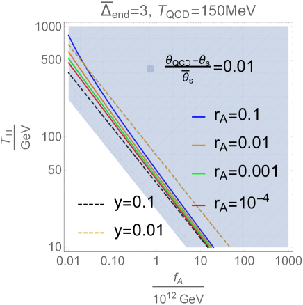
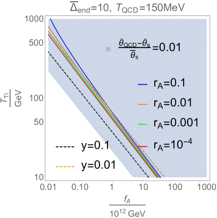
Figure 4: The CMB amplitude $A_{s}$ is explained if $\overline{H}_{\rm exit}$ is appropriately chosen as in Eq.(82). On each solid line, a different value of $r_{A}$ in Eq. (81) is predicted, which is constrained by the isocurvature constraint of Eq.(44). Other parameters are set as $(\overline{\theta}_{\rm QCD}-\overline{\theta}_{S})/\overline{\theta}_{S}=0.01$, and $\overline{\Delta}_{\rm end}=3\ (10)$ in the Left (Right) panel. If the parameters are in the blue regions, the non-Gaussianity constraint Eq. (24) is satisfied. We also plot $y\simeq\eta/30.2$ to see why a small value of $r_{A}$ in Eq. (81) is realizable. The dashed black (orange) line corresponds to $y=0.1\ (0.01)$. The figure shows that the three conditions in section 3.2 can be satisfied in the thermal inflation scenario.

In Fig.4, we plot the prediction of axion abundance $r_{A}$ as a function of two parameters $(T_{\rm TI},f_{A})$. The scalar amplitude $A_{s}$ in Eq.(70) explains the CMB anisotropy if $\overline{H}_{\rm exit}$ is chosen as

$$\left(1-y\cos(\bar{\theta}_{\rm QCD})\right)\sin(\bar{\theta}_{\rm QCD})\times\frac{\overline{H}_{\text{exit}}(k_{*})}{\pi f_{A}}\simeq 0.03\times\left(\frac{T_{\rm QCD}}{150{\rm MeV}}\right)^{4}~{}.$$ (82)

On each line, the model predicts a different value of $r_{A}$, which is constrained by the condition of isocurvature fluctuations in Eq.(44). In the left (right) panel, we set the e-folding of thermal inflation between the QCD phase transition until the end of the thermal inflation as $\overline{\Delta}_{\rm end}=3\ (10)$. We further set the angle $\bar{\theta}_{\rm QCD}$ to take $(\overline{\theta}_{\rm QCD}-\overline{\theta}_{S})/\overline{\theta}_{S}=0.01$. Then the non-Gaussianity constraint Eq. (24) is satisfied if the parameters are in the blue region. Any tiny value of $r_{A}$ can be obtained by tuning the parameters on the solid lines. This is because $y\simeq\eta/30.2$ can take a larger value by choosing the parameters, as plotted by the dashed lines; we represent the $y\simeq\eta/30.2=0.1\ (0.01)$ contours by dashed black (orange) lines. Thus all of the three conditions in 3.2 can be satisfied. The difficulties of the standard QCD axion scenario are evaded because the axion never starts to oscillate during the thermal inflation because the condition $3H_{\rm TI}>m_{A}(T)$ is always satisfied in this parameter region. Thus, the thermal inflation scenario can meet the necessary conditions discussed in Section 3 provided the inflation lasts long enough below the QCD phase transition.

Finally we comment on the non-Gaussianity of isocurvature fluctuations. One can evaluate isocurvature contributions to the non-Gaussianity of the gravitational potential introduced in Appendix A by using the evolution of $\theta$ in Eq.(76) between the QCD and end slices, as well as the one after the thermal inflation. As discussed in Appendix D (in particular in Eqs. (141)(142)), the effect turns out to be very small since the isocurvature perturbation is tiny compared to the adiabatic one. Thus the observational constraints for isocurvature non-Gaussianity can be easily evaded.

4.3 $B$-$L$ model with QCD axion

In the final section, we briefly comment on a classically conformal $B$-$L$ model [61, 62, 63, 64] with QCD axion because it has a potential to avoid difficulties in the standard QCD. A novel feature of the model is that, due to the assumption of the classical conformality (i.e. absence of quadratic terms in the scalar potential), the universe has experienced an era of supercooling for both of the $B$-$L$ and the electroweak symmetries [64]: these symmetries are not spontaneously broken until the chiral symmetry breaking $\langle\bar{\psi}\psi\rangle\neq 0$ occurs at the QCD temperature. Also the vacuum energy of a scalar field with a $B$-$L$ charge generates thermal inflation from TeV to QCD scales. Once $\langle\bar{\psi}\psi\rangle$ acquires a non-zero value, a linear term in the Higgs potential is generated through the Yukawa coupling $yh\bar{\psi}\psi$. Thus, the electroweak symmetry breaking occurs at $T_{\rm QCD}$, but with a smaller vev $\langle h\rangle\sim{\cal O}(\Lambda_{\rm QCD})$ than the electroweak scale. As the temperature of the universe further goes down, $B$-$L$ symmetry is then spontaneously broken by a scalar mixing of the SM Higgs $h$ and $B$-$L$ scalar field $\phi_{\rm B\text{-}L}$, and then the SM Higgs acquires an ordinary vev at $\langle h\rangle=246$ GeV. Due to the vacuum energy $V(\phi_{\rm B\text{-}L})$ of the $B$-$L$ scalar $\phi_{\rm B\text{-}L}$, thermal inflation continues until the end of the supercooling era, which is below $T_{\rm QCD}$. Therefore, the scenario investigated in the previous section is naturally realized: axions are diluted in the thermal inflation to have a small value of $r_{A}$. This model provides a natural scenario for the thermal inflation below the QCD scale, and the classically conformal $B$-$L$ model with the QCD-like axion can be a good candidate for the scenario to explain CMB anisotropy by the axion isocurvature fluctuations. But there is one technical difficulty to obtain a large value of $R$ since quark masses are smaller than usual when the axion potential is generated, due to the smallness of $\langle h\rangle$ at $T=T_{\rm QCD}$, and the axion energy density becomes smaller than the scenario in the previous section. In order to overcome this difficulty in generating sufficient amount of fluctuations, we need to raise the axion potential, e.g., by introducing a mixing of the SM Higgs and axions. Further studies of modifications of the model are left for future publications.

5 Conclusions

In this paper, we have investigated a possibility to explain the CMB anisotropy by the primordial fluctuations of QCD-like axions. Such a scenario is generally characterized by three parameters, amplitude of the axion fluctuation $\overline{H}_{\rm exit}/f_{A}\bar{\theta}_{\rm ini}$, ratio of energy densities of axion to radiation $R=\Omega_{A}/\Omega_{r}$ when the axion potential is generated, and the fraction of the present axion abundance $r_{A}=\Omega_{A}/\Omega_{\rm CDM}|_{\rm today}$. In order to be consistent with the CMB observations, especially the non-Gaussianity and isocurvature constraints, we need $0.01\lesssim R\leq 1$ and simultaneously a small value of $r_{A}$. It is summarized in Fig. 3. To realize these values, a certain dilution mechanism of axions after $T_{\rm QCD}$ is inevitable, and a natural possibility is the thermal inflation that lasts below the QCD scale. Specifying the thermal inflation model by its Hubble parameter $H_{\rm TI}$ (or its corresponding temperature $T_{\rm TI}$) and the number of e-folding $\overline{\Delta}_{\rm end}$ from $T_{\rm QCD}$ to the end of the thermal inflation, we obtain the allowed parameter region of the thermal inflation model shown in Fig.4. In this investigations, we have taken important effects of non-Gaussianity from the axion potential itself and from the evolutions of the axion field before and after the QCD phase transition, denoted respectively by ${\cal X},{\cal Y}$ and ${\cal Z}$. In order to evade the non-Gaussianity constraint for $f_{\rm NL}$, the axion angle at the QCD scale must be $\overline{\theta}_{\rm QCD}\simeq\pi/2$. It is interesting then that the non-Gaussianity $g_{\rm NL}$ becomes within reach of observations in near-future.

An interesting prediction of the axion scenario for the CMB anisotropy is that, as noted in the footnote 5, since the axion field did not have potential when its fluctuation is generated during the primordial inflation, the spectral index $n_{s}=1-2\epsilon$ coincides with the tensor mode index $n_{t}$. Thus, when the tensor mode is discovered and its spectral index is observed, we can justify/falsify our model.

As a concrete model of a such thermal inflation scenario, we comment on a classically conformal $B$-$L$ model. This model naturally realizes thermal inflation at very low energy scale and can be a good candidate. However, there is a technical difficulty to obtain sufficient amount of the CMB fluctuations. To overcome this difficulty, we need to raise the height of the axion potential, and accordingly the amplitude of the Higgs vev when the QCD phase transition occurs than $\langle v\rangle\sim{\cal O}(\Lambda_{\rm QCD})$. It may be possible by generating a negative thermal mass term of the Higgs from interactions with other scalar fields. We want to come back to this model in future investigations.

Appendix Appendix A Curvature perturbations and CMB observables

In this appendix, we discuss how the gauge invariant curvature perturbations are related to the CMB observables in $\Lambda$CDM model. In the following, we consider only linear perturbations for simplicity. Assume there are two CDM components; one ($d$) is produced from the SM radiation in the early universe and the other ($A$ for axion) is essentially decoupled from the SM in late time. After the Big-Bang Nucleosynthesis, each of these CDMs, the SM baryon ($b$) and photon ($\gamma$) are described as a perturbed perfect fluid with

$$w_{\gamma}=\frac{1}{3}~{}~{},~{}~{}~{}w_{b}=w_{d}=w_{A}=0~{},$$ (83)

$$\zeta_{r}^{(1)}:=\zeta_{\gamma}^{(1)}=\zeta_{b}^{(1)}=\zeta_{d}^{(1)}~{}~{},~{}~{}~{}\zeta_{A}^{(1)}\neq\zeta_{r}^{(1)}~{}.$$ (84)

The matter dominated era starts at $T=T_{\rm eq}\sim{\rm eV}$ and the last scattering surface is given at $T=T_{\rm lss}\sim 0.1$eV. The dark energy fraction $\Omega_{\Lambda}$ is still totally negligible and the curvature perturbation Eq. (10) is given by

$$\zeta^{(1)}=\frac{(4\Omega_{\gamma}+3\Omega_{b}+3\Omega_{d})\zeta_{\gamma}^{(1)}+3\Omega_{A}\zeta_{A}^{(1)}}{4\Omega_{\gamma}+3\Omega_{b}+3\Omega_{d}+3\Omega_{A}}\bigg{|}_{\text{lss}}=\zeta_{\gamma}^{(1)}-\zeta_{\gamma,{\rm iso}}^{(1)}$$ (85)

where

$$\zeta_{\gamma,{\rm iso}}^{(1)}= \frac{\Omega_{A}}{3\Omega_{m}+\Omega_{\gamma}}\bigg{|}_{\text{lss}}S_{A}\simeq\frac{\Omega_{A}}{3\Omega_{m}}\bigg{|}_{\text{lss}}S_{\rm A}=\frac{\Omega_{A}}{3\Omega_{m}}\bigg{|}_{\text{today}}S_{\rm A},~{}~{}S_{\rm A}:=-3(\zeta_{\rm A}^{(1)}-\zeta_{\gamma}^{(1)})~{}.$$ (86)

Here, $\Omega_{m}:=\Omega_{b}+\Omega_{d}+\Omega_{A}=\Omega_{\rm CDM}+\Omega_{A}$ is the total matter energy density fraction and the ratio $\Omega_{A}/\Omega_{m}$ can be evaluated at the present time because it does not change much through the time evolution of the universe. If the integrated Sachs-Wolfe contribution is neglected, the CMB temperature anisotropy is given by a simple analytic expression as [33, 73]

$$\frac{\delta T}{T}=-\zeta_{\gamma}^{(1)}-2\Phi^{(1)}\bigg{|}_{\rm lss}$$ (87)

with the gravitational potential $\Phi$ which is, in the matter dominated era, approximated as

$$\Phi\simeq-\frac{3}{5}\zeta~{}.$$ (88)

Plugging this and Eq. (85) into Eq. (87), we find

$$\frac{\delta T}{T}=-\zeta_{\gamma}^{(1)}+\frac{6}{5}\zeta^{(1)}\bigg{|}_{\rm lss}=\frac{1}{5}\zeta_{\gamma}^{(1)}-\frac{6}{5}\zeta_{\gamma,{\rm iso}}^{(1)}\bigg{|}_{\rm lss}~{},$$ (89)

which shows that the isocurvature component affects the CMB anisotropy via the gravitational potential at the last scattering. With the definition of ${\cal R}$ and ${\cal I}$ given in (15), the observation of the two point function of the temperature perturbation gives the constrains (19), (22) and (23).

Furthermore, the Planck experiment gives constraints on the three point function of the gravitational potential as follows. Here, (88) is divided into to parts as $\Phi=\Phi^{\rm a}+\Phi^{\rm i}$ where

$$\Phi^{a}:=\frac{3}{5}{\cal R}~{}~{}~{},~{}~{}~{}~{}\Phi^{\rm i}:=\frac{r_{c}}{5}{\cal I}$$ (90)

with $r_{c}:=[\Omega_{\rm CDM}+\Omega_{b}]_{\rm today}\simeq 0.842$. In general, both can be significant in the three point function [74, 75, 56, 76, 77]. Each component is expanded as

$$\Phi^{J}=\Phi^{J}_{u}\delta\phi^{u}+\frac{\Phi^{J}_{uv}}{2}\delta\phi^{u}\delta\phi^{v}+\cdots$$ (91)

with the repeated indices $u,v$ summed over scalar (inflaton and axion) fields $\phi^{u}=(\sigma,A)$ which acquire the almost scale invariant spectrum during the primordial inflation. The local type bispectrum $B^{IJK}$ is defined by

$$\langle\Phi^{I}(k_{1})\Phi^{J}(k_{2})\Phi^{K}(k_{3})\rangle=(2\pi)^{3}\delta^{(3)}(k_{1}+k_{2}+k_{3})B^{IJK}(k_{1},k_{2},k_{3})~{},$$ (92)

$$B^{IJK}(k_{1},k_{2},k_{3})=2f^{I,JK}_{\rm NL}P_{\Phi}(k_{2})P_{\Phi}(k_{3})+2f^{J,KI}_{\rm NL}P_{\Phi}(k_{3})P_{\Phi}(k_{1})+2f^{K,IJ}_{\rm NL}P_{\Phi}(k_{1})P_{\Phi}(k_{2})~{},$$ (93)

normalized in terms of the power spectrum

$$P_{\Phi}(k)\simeq\frac{2\pi^{2}}{k^{3}}\times\frac{H^{2}}{4\pi^{2}}(\Phi^{\rm a}_{u}\Phi^{\rm a}_{u})=\frac{2\pi^{2}}{k^{3}}\times\frac{9A_{s}}{25}~{},$$ (94)

where the isocurvature mode is assumed to have a negligible contribution to the power spectrum to be consistent with the observation that $\beta_{\rm iso}\ll 1$. Then, the six independent non-linear parameters [78, 79] are given as

$$f^{I,JK}_{\rm NL}=\frac{\Phi^{I}_{uv}\Phi^{J}_{u}\Phi^{K}_{v}}{2(\Phi^{\rm a}_{u^{\prime}}\Phi^{\rm a}_{u^{\prime}})^{2}}~{}.$$ (95)

When only one scalar field (axion $A$ in our case) contributes to the large scale perturbation, we find

$$f^{\rm a,aa}_{\rm NL}=\frac{5}{6}\frac{{\cal R}_{AA}}{{\cal R}_{A}^{2}}~{},$$ (96)

which corresponds to the coefficient $f_{\rm NL}$ of the second order term in the expansion (14). From Table 7 in [3], we see that the constraint on this purely adiabatic component is the most stringent and given in Eq. (24).

Appendix Appendix B Gradual energy transfer taken into account

In the body of paper, it is assumed that the energy transfer between the radiation and the axion field occurs all at once on the transition slice characterized by $T=T_{A}$ for brevity. Here, let us consider a more realistic process of gradual energy transfer focusing on the standard QCD axion scenario with $T_{A}=T_{\rm QCD}$. We will find that the gradual energy transfer does not change our conclusion so much.

In the following, thermal history is divided into several stages by time slices on which the discontinuities take place. For completeness, we start from the horizon exit of the CMB scale during the primordial inflation, stage (I). Assuming the reheating is instantaneous, we have the radiation dominated era with (I​I) $T>T_{\rm EW}$, (I​I​I) $T_{\rm EW}>T>T_{\rm osc}$, (I​V) $T_{\rm osc}>T>T_{\rm QCD}$ and (V) $T<T_{\rm QCD}$. And the four time slices connecting the stages are called, reheating (rh), electroweak (EW), oscillation (osc) and QCD slice, respectively, see Fig.5. The total energy density $\rho$ and the spacetime metric, especially $\psi$, are continuous on each slices.

For the standard QCD axion scenario, we are particularly interested in $\rho_{r}$ and $S_{A}=-3(\rho_{A}-\rho_{r})$ in the last stage (V). The former is nothing but $-\psi$ on a uniform temperature slice by definition and the latter is given as the perturbation of $\rho_{A}$ on a uniform temperature slice after the QCD transition, as discussed around (39).

Figure 5: Thermal history of standard QCD axion scenario. The horizontal axis represents the direction of time evolution.

(I) Primordial inflation

The total energy is stored in the inflaton field $\sigma$ in this stage: $\rho=\rho_{\sigma}$. Inflaton’s equation of motion is $(-g)^{-1/2}\partial_{\mu}\left\{(-g)^{1/2}g^{\mu\nu}\partial_{\nu}\sigma\right\}=\partial_{\sigma}V_{\sigma}$ with $V_{\sigma}$ being inflaton’s potential. Dropping the second time derivative, we get the slow-roll equation in the metric (1) as

$$3H\dot{\sigma}/\lambda\simeq-\partial_{\sigma}V_{\sigma}$$ (97)

where $H^{2}\simeq V_{\sigma}/3m_{\rm Pl}^{2}$ and the dot denotes $t$-derivative. Since the energy density and the pressure density are given as $\rho_{\sigma}\simeq(\dot{\sigma}/\lambda)^{2}/2+V_{\sigma}$ and $P_{\sigma}\simeq(\dot{\sigma}/\lambda)^{2}/2-V_{\sigma}$ in the superhorizon limit, the EOS is now approximated as $w_{\sigma}\simeq-1+2\epsilon/3$ where $\epsilon:=\left(m_{\rm Pl}\partial_{\sigma}\ln V_{\sigma}\right)^{2}/2$ is the first slow-roll parameter.

On the initial “exit” slice, $\psi_{\rm exit}=0$ is assumed. Following the definition (6), we obtain

$$\zeta_{\rm inf}\simeq-\psi_{\rm exit}-\int^{\sigma_{\rm exit}}_{\bar{\sigma}_{\rm exit}}\frac{d\sigma V_{\sigma}^{\prime}}{2\epsilon V_{\sigma}}=-{\rm sign}(V_{\sigma}^{\prime})\int^{\sigma_{\rm exit}}_{\bar{\sigma}_{\rm exit}}\frac{d\sigma/m_{\rm Pl}}{\sqrt{2\epsilon}}$$ (98)

which conserves until the end of the inflation characterized by $\epsilon=1$. Therefore, this “reheating” slice is nothing but a uniform $\rho_{\sigma}$ slice on which

$$\psi_{\rm rh}=-\zeta_{\rm inf}~{}.$$ (99)

During this stage, axion’s primordial large scale fluctuations (32) are also generated. However, it is assumed that its potential is still absent and the field value does not evolve.

(I​I) $T>T_{\rm EW}$ radiation domination

On the reheating slice, it is assumed that all the energy density is converted to radiation’s energy density: $\rho=\rho_{r}$, and then, the curvature perturbation (98) is copied, via (99), into the radiation:

$$\zeta_{r}=-\psi_{\rm rh}$$ (100)

which is constant throughout this stage ending at $T=T_{\rm EW}$. On this “EW” slice, the temperature is constant:

$$\delta\rho|_{\rm EW}=\delta\rho_{r}|_{\rm EW}=0~{},$$ (101)

and hence, we have

$$\psi_{\rm EW}=-\zeta_{r}=\psi_{\rm rh}~{}.$$ (102)

Regarding the axion field, its potential is still absent and the field value does not evolve with time. And the perturbation $\delta A$ does not depend on the choice of time slice.

(I​I​I) $T_{\rm EW}>T>T_{\rm osc}$

The axion acquires the temperature dependent potential (50) which is, however, too small to drive the field value to roll down to the minimum. We simply assume $\dot{A}=0$, and thus, $w_{A}=-1$ in this stage. Then, $\rho_{A}=V_{A}$, we have

$$\dot{\rho}_{A}=+\dot{T}\partial_{T}V_{A}=+8b\dot{\tau}V_{A}~{},$$ (103)

where $\tau:=-\ln T/T_{\rm ref}$ with an arbitrary reference temperature $T_{\rm ref}$. By the energy conservation,

$$\dot{\rho}_{r}+4\lambda H\rho_{r}=-8b\dot{\tau}V_{A}$$ (104)

holds. We now solve it with respect to $\tau$. With the local $e$-folding number $N=\int dt\lambda H$, the above equation is rewritten as

$$dN=d\tau\left[1-2bx_{0}e^{(8b+4)\tau}\right]~{},$$ (105)

where $x:=\rho_{A}/\rho_{r}\propto e^{(8b+4)\tau}$ and $x_{0}=x|_{\tau=0}$. Integrating it from the EW slice to the “oscillation” slice where $m_{A}/3H=1$, we have

$$N_{\rm osc}-N_{\rm EW} = \int^{\tau_{\rm osc}}_{\tau_{\rm EW}}d\tau\left[1-2bx_{0}e^{(8b+4)\tau}\right]$$

$$= \tau_{\rm osc}-\tau_{\rm EW}-\frac{b/4}{b+1/2}\left[x_{\rm osc}-x_{\rm EW}\right]~{}.$$

If tiny values of $x$ are neglected, this is nothing but $T\propto a^{-1}$ and $x\propto a^{8b+4}$.

The boundary condition on the EW slice (101) becomes, in this stage,

$$\delta\rho|_{\rm EW}=\delta\rho_{r}|_{\rm EW}+\delta\rho_{A}|_{\rm EW}=0~{},$$ (107)

which is equivalent to

$$\delta\tau_{\rm EW}=\frac{x_{\rm EW}/4}{1-2bx_{\rm EW}}\left.\frac{\delta V_{A0}}{V_{A0}}\right|_{\rm exit}~{}.$$ (108)

On the other hand, on the oscillation slice, perturbations should satisfy $\delta(m_{A}/3H)=0$, which is to say,

$$\left[\frac{\delta\rho_{r}}{\rho_{r}}+\frac{x}{1+2b/z}\frac{\delta\rho_{A}}{\rho_{A}}\right]_{\rm osc}=0$$ (109)

with $z:=\rho_{r}/\rho=(1+x)^{-1}$. This is equivalent to

$$\delta\tau_{\rm osc}=\frac{z_{\rm osc}x_{\rm osc}/4}{2b+z_{\rm osc}(1-2bx_{\rm osc})}\left.\frac{\delta V_{A0}}{\bar{V}_{A0}}\right|_{\rm exit}~{}.$$ (110)

By differentiating (Appendix B), we obtain “$\delta N$” as, to linear order,

$$\psi_{\rm osc}-\psi_{\rm EW} = \left[1-2bx_{\rm osc}\right]\times\delta\tau_{\rm osc}-\left[1-2bx_{\rm EW}\right]\times\delta\tau_{\rm EW}$$ (111)

$$-\frac{b/4}{b+1/2}\left[x_{\rm osc}-x_{\rm EW}\right]\times\left.\frac{\delta V_{A0}}{V_{A0}}\right|_{\rm exit}$$

$$\simeq -\frac{b-1/2}{b+1/2}\frac{\bar{x}_{\rm osc}}{4}\times 2\left.\frac{\delta A}{\bar{A}}\right|_{\rm exit}~{}.$$

On the last line, terms with $\bar{x}_{\rm EW}\ll\bar{x}_{\rm osc}$ are omitted.

(I​V) $T_{\rm osc}>T>T_{\rm QCD}$

In this stage, we assume the separation of two time scales; the frequency of axion’s coherent oscillation is much larger than its changing rate. Then, the time-averaging commutes with the partial $t$-derivative acting on the potential: $\langle\partial_{t}V_{A}\rangle_{t}=\partial_{t}\langle V_{A}\rangle_{t}=\dot{T}\partial_{T}\langle V_{A}\rangle_{t}$. It is also assumed that $V_{A}$ is well approximated by a harmonic form, and then, $w_{A}=0$ and $\rho_{A}=2\langle V_{A}\rangle_{t}$. Therefore, we have

$$\dot{\rho}_{A}+3\lambda H\rho_{A}=+\dot{T}\langle\partial_{T}V_{A}\rangle_{t}=+4b\dot{\tau}_{A}\rho_{A}~{},$$ (112)

and from the energy conservation,

$$\dot{\rho}_{r}+4\lambda H\rho_{r}=-4b\dot{\tau}_{A}\rho_{A}~{}.$$ (113)

The second equation (113) is written as

$$d\tau/dN=(1-bx)^{-1}~{}.$$ (114)

By eliminating $d\tau/dN$ from (112), we get

$$dN=\frac{dx}{x}\frac{(1-bx)}{1+b(4+3x)}~{},$$ (115)

and combining this with (114),

$$d\tau=\frac{dx}{x}\frac{1}{1+b(4+3x)}~{}.$$ (116)

These equations are integrated from the oscillation slice to the QCD slice as

$$N_{\rm QCD}-N_{\rm osc}=\frac{1}{1+4b}\left[\ln\frac{x_{\rm QCD}}{x_{\rm osc}}-\frac{4(1+b)}{3}\ln\frac{1+b(4+3x_{\rm QCD})}{1+b(4+3x_{\rm osc})}\right]~{},$$ (117)

$$\tau_{\rm QCD}-\tau_{\rm osc}=\frac{1}{1+4b}\left[\ln\frac{x_{\rm QCD}}{x_{\rm osc}}-\ln\frac{1+b(4+3x_{\rm QCD})}{1+b(4+3x_{\rm osc})}\right]~{}.$$ (118)

If tiny values of $x$ are set to zero in the second terms, one finds $T\propto a^{-1}$ and $\rho_{A}\propto a^{4b-3}$ which is consistent with (53).

On the oscillation slice, the sudden change of axion’s EOS occurs. Then, we have (110), and equivalently,

$$\frac{\delta x_{\rm osc}}{x_{\rm osc}}=\frac{1+x_{\rm osc}+2b/z_{\rm osc}}{x_{\rm osc}/4}\times\delta\tau_{\rm osc}~{}.$$ (119)

On the QCD slice, the boundary condition is simply given by

$$\delta\rho_{r}|_{\rm QCD}=0~{},$$ (120)

therefore,

$$\delta\tau_{\rm QCD}=0~{}~{}~{},~{}~{}~{}~{}\left.\frac{\delta x}{x}\right|_{\rm QCD}=\left.\frac{\delta V_{A0}}{V_{A0}}\right|_{\rm QCD}~{}.$$ (121)

Differentiating (118) with respect to $\tau$ and $x$, we find

$$\left.\frac{\delta V_{A0}}{V_{A0}}\right|_{\rm QCD} = \left\{1+b(4+3x_{\rm QCD})\right\}\left[\frac{\delta x/x}{1+b(4+3x)}-\delta\tau\right]_{\rm osc}$$ (122)

$$\simeq \frac{1+b(4+3R)}{1+4b}\left.\frac{\delta V_{A0}}{\bar{V}_{A0}}\right|_{\rm exit}~{},$$

where $R:=\bar{x}_{\rm QCD}\ll 1$. On the second line, only the first order of $\delta$ is retained, and then, $\bar{x}_{\rm osc}\ll R$ is neglected. And by differentiating (117), we obtain “$\delta N$” as, to linear order,

$$\psi_{\rm QCD}-\psi_{\rm osc} = \left[\frac{\delta x}{x}\frac{(1-bx)}{1+b(4+3x)}\right]^{\rm QCD}_{\rm osc}$$ (123)

$$\simeq -\frac{bR}{1+4b}\times 2\left.\frac{\delta A}{\bar{A}}\right|_{\rm exit}~{}.$$

(V) $T_{\rm QCD}>T$

Here, we do not consider the vacuum energy to be released on the QCD phase transition. Then, only the time derivative of axion’s potential gets discontinuity. Since it is the uniform temperature slice, we have $\delta\rho_{r}|_{\rm QCD}=0$ and, to linear order,

$$\zeta_{r} = -\psi_{\rm QCD}=-(\psi_{\rm QCD}-\psi_{\rm osc})-(\psi_{\rm osc}-\psi_{\rm EW})-\psi_{\rm EW}$$ (124)

$$\simeq \zeta_{\rm inf}+\frac{2bR}{1+4b}\left.\frac{\delta A}{\bar{A}}\right|_{\rm exit}~{}.$$

On the second line, the contribution (111) proportional to $\bar{x}_{\rm osc}$ is neglected. Comparing this with (29) for the harmonic case ${\cal X}_{\rm a}=1$, we find the coefficient of $[\delta A/\bar{A}]_{\rm exit}$ now smaller by a factor $4b/(4b+1)$. The instantaneous energy transfer limit corresponds to $b\to\infty$, and then, this factor goes to unity as expected.

As for axion’s fluctuation, since $w_{A}=0$ and there is no longer energy transfer in this stage, the evolution equation is linear and $\delta A/A$ conserves. Then, from (122), we find

$$\left.\frac{\delta V_{A0}}{V_{A0}}\right|_{\rm late~{}time}=\left.\frac{\delta V_{A0}}{V_{A0}}\right|_{\rm QCD}\simeq\frac{1+b(4+3R)}{1+4b}\left.\frac{\delta V_{A0}}{\bar{V}_{A0}}\right|_{\rm exit}~{}.$$ (125)

Note that the factor ${\cal X}_{\rm i}=1+3R/4$ mentioned above (56) is correctly reproduced in the instantaneous limit.

Appendix Appendix C Curvature perturbations in thermal inflation scenario

In this appendix, we briefly discuss how the gradual energy transfer is taken into account in computing the curvature perturbation generated at the QCD transition during the thermal inflation, and how it is converted to the final one of radiation we observe today. We assume that all of the vacuum energy $V_{\rm TI}=(g_{\rm TI}\pi^{2}/30)T_{\rm TI}^{4}$ which drives the thermal inflation is suddenly converted to the energy density $\rho_{\phi}$ of a scalar field $\phi$ oscillating with its EOS $w_{\phi}=0$. And subsequently, this coherent oscillation suddenly decays to the radiation once the Hubble expansion rate drops to satisfy $3H=\Gamma_{\phi}$ with $\Gamma_{\phi}$ being a constant decay rate of the scalar field: the gradual energy transfer from the oscillation to the radiation is neglected for simplicity since it is not our main focus here.

Let us apply the analysis in Appendix B to the thermal inflation scenario where, typically, the axion field does not oscillate around the potential minimum during the thermal inflation. Note that the considerations in Appendix B are all valid regardless of the dominant component (apart from $z=1-x$ introduced in (109) which is now irrelevant). We can integrate the evolution equations (103) and (104) from the EW slice to the QCD slice on which $\delta\rho_{r}|_{\rm QCD}=0$, hence, Eq. (121). Then, instead of Eq. (111), we obtain, to linear order,

$$\zeta_{r,{\rm TI}}\simeq\psi_{\rm QCD}-\psi_{\rm EW}\simeq-\frac{b}{b+1/2}\frac{R}{4}\times\left.\frac{\delta V_{A0}}{\bar{V}_{A0}}\right|_{\rm exit}~{},$$ (126)

as the dominant contribution to the uniform temperature curvature perturbation after the QCD transition during the thermal inflation $\zeta_{r,{\rm TI}}$. Compared with Eq. (29), this is smaller by a factor $b/(b+1/2)$ which goes to unity in the instantaneous energy transfer limit $b\to\infty$.

Since the thermal inflation ends on the uniform temperature slice characterized by $T=T_{\rm end}$, scale factor’s perturbation on this “end” slice is given as

$$\psi_{\rm end}=-\zeta_{r,{\rm TI}}~{}.$$ (127)

From the assumption, we have

$$V_{0}=\rho_{\phi}|_{\rm end}~{}.$$ (128)

Therefore, $\rho_{\phi}=\bar{\rho}_{\phi}\exp(-3(\zeta_{\phi}+\psi))$ is uniform on this slice, and thus,

$$\zeta_{\phi}=-\psi_{\rm end}$$ (129)

to conserve until $\phi$’s decay. On the “decay” slice, the Hubble rate is uniform. In other words,

$$\delta\rho|_{\rm decay}=0~{}.$$ (130)

We further assume that the energy density is dominated by the coherent oscillation before this slice. This is actually the case with the sufficiently long thermal inflation discussed in Section 4.2. Then, $\Omega_{\phi}\simeq 1$ and all the other contributions are negligible in the curvature perturbation Eq. (10). Therefore, we get

$$\psi_{\rm decay}\simeq-\zeta_{\phi}~{}.$$ (131)

After the decay slice, the radiation as the decay product is dominant component. Therefore,

$$\zeta_{r,{\rm decay}}\simeq-\psi_{\rm decay}\simeq\zeta_{\phi}=-\psi_{\rm end}=\zeta_{r,{\rm TI}}~{},$$ (132)

that is to say, if the thermal inflation lasts long enough, the curvature perturbation associated with the radiation existing during the thermal inflation is copied to the one after the reheating.

Provided that the temperature of this decay product is higher than the EW one, we can follow the discussion in Appendix B but now with $\zeta_{r,{\rm decay}}$ replacing $\zeta_{\rm inf}$. Neglecting the tiny value of $R:=\bar{x}_{\rm QCD}$ in the standard thermal history realized after the thermal inflation, we finally obtain the observable one as $\zeta_{r}\simeq\zeta_{r,{\rm decay}}\simeq\zeta_{r,{\rm TI}}$.

Appendix Appendix D Isocurvature non-Gaussianity

In order to evaluate the non-Gaussianity from the isocurvature perturbations as well as its power spectrum, axion’s evolution equation is integrated from the QCD slice to the end slice, resulting in Eq. (77) for a sufficiently large e-folding number $\Delta_{\rm end}$. With $\theta_{\rm end}\ll 1$, the evolution after the end of the thermal inflation is almost linear, and thus, we have $[\delta\theta/\bar{\theta}]_{\rm late~{}time}\simeq[\delta\theta/\bar{\theta}]_{\rm end}$ in Eq. (39) and

$$S_{A}\simeq 2\frac{\delta\theta_{\rm end}}{\bar{\theta}_{\rm end}}-\left(\frac{\delta\theta_{\rm end}}{\bar{\theta}_{\rm end}}\right)^{2}+\cdots~{},$$ (133)

where the second order term is also retained since, in the following, we compute the nonlinear parameters defined by Eq. (95). Let us remember that the non-Gaussianity of the purely adiabatic component Eq. (71) is enhanced by $1/R$, as in Eq.(35). This is also the case in other components. Here, we focus on the largest power of $1/R$ for each of $\Phi^{\rm a,i}_{\theta}$ and $\Phi^{\rm a,i}_{\theta\theta}$.

The isocurvature contribution to the gravitational potential defined in Eq. (90) is given as

$$\Phi^{\rm i}\simeq\Phi^{\rm i}_{\theta}\delta\theta_{\rm ini}+\frac{\Phi^{\rm i}_{\theta\theta}}{2}\delta\theta_{\rm ini}^{2}+{\cal O}(\delta\theta_{\rm ini}^{3})~{},$$ (134)

$$\Phi^{\rm i}_{\theta}=\overline{\frac{\delta\theta_{\rm QCD}}{\delta\theta_{\rm ini}}}\Phi^{\rm i}_{\theta,{\rm QCD}}~{},~{}~{}~{}~{}\Phi^{\rm i}_{\theta\theta}=\left(\overline{\frac{\delta\theta_{\rm QCD}}{\delta\theta_{\rm ini}}}\right)^{2}\Phi^{\rm i}_{\theta\theta,{\rm QCD}}+\overline{\frac{\delta^{2}\theta_{\rm QCD}}{\delta\theta_{\rm ini}^{2}}}\Phi^{\rm i}_{\theta,{\rm QCD}}~{},$$

where

$$\Phi^{\rm i}_{\theta,{\rm QCD}}:=\frac{r_{A}r_{c}}{5}\overline{\frac{2}{\theta_{\rm end}}\frac{\delta\theta_{\rm end}}{\delta\theta_{\rm QCD}}}=\frac{r_{A}r_{c}}{5}\frac{2{\cal Z}(\bar{\theta}_{\rm QCD})}{\bar{\theta}_{\rm QCD}}\simeq\frac{r_{A}r_{c}}{5}\frac{2}{\sin(\bar{\theta}_{\rm QCD})}~{},$$

$$\Phi^{\rm i}_{\theta\theta,{\rm QCD}}:=\frac{r_{A}r_{c}}{5}\overline{\frac{\delta}{\delta\theta_{\rm QCD}}\left(\frac{2}{\theta_{\rm end}}\frac{\delta\theta_{\rm end}}{\delta\theta_{\rm QCD}}\right)}\simeq\frac{r_{A}r_{c}}{5}\frac{-2\cos(\bar{\theta}_{\rm QCD})}{\sin^{2}(\bar{\theta}_{\rm QCD})}~{}.$$

Note that, in evaluating the approximate equalities, ${\cal O}(R)$ term are omitted. See the discussion around Eq. (79). Similarly, the adiabatic contribution to the gravitational potential is given as

$$\Phi^{\rm a} \simeq \Phi^{\rm a}_{\theta}\delta\theta_{\rm ini}+\frac{\Phi^{\rm a}_{\theta\theta}}{2}\delta\theta_{\rm ini}^{2}+{\cal O}(\delta\theta_{\rm ini}^{3})~{},$$ (135)

$$\Phi^{\rm a}_{\theta}=-\frac{3}{5}\frac{\delta\zeta_{r{\rm G}}}{\delta\theta_{\rm ini}}=\overline{\frac{\delta\theta_{\rm QCD}}{\delta\theta_{\rm ini}}}\Phi^{\rm a}_{\theta,{\rm QCD}}~{},$$

$$\Phi^{\rm a}_{\theta\theta}=2\left(\Phi^{\rm a}_{\theta}\right)^{2}f_{\rm NL}(\bar{\theta}_{\rm QCD},y)=\left(\overline{\frac{\delta\theta_{\rm QCD}}{\delta\theta_{\rm ini}}}\right)^{2}\Phi^{\rm a}_{\theta\theta,{\rm QCD}}+\overline{\frac{\delta^{2}\theta_{\rm QCD}}{\delta\theta_{\rm ini}^{2}}}\Phi^{\rm a}_{\theta,{\rm QCD}}~{},$$

where

$$\Phi^{\rm a}_{\theta,{\rm QCD}}:=-\frac{3}{5}\frac{R{\cal X}(\bar{\theta}_{\rm QCD})}{2\bar{\theta}_{\rm QCD}}=-\frac{3}{5}\frac{R}{4}\frac{\sin(\bar{\theta}_{\rm QCD})}{1-\cos(\bar{\theta}_{\rm QCD})}~{},$$

$$\Phi^{\rm a}_{\theta\theta,{\rm QCD}}:=2\left(\Phi^{\rm a}_{\theta,{\rm QCD}}\right)^{2}f_{\rm NL}(\bar{\theta}_{\rm QCD},0)\simeq-\frac{3R}{20}\frac{\cos(\bar{\theta}_{\rm QCD})}{1-\cos(\bar{\theta}_{\rm QCD})}~{}.$$ (136)

Comparing Eq. (134) and Eq. (135), one finds

$$\Phi^{\rm i}_{\theta}=-{\cal W}\times\Phi^{\rm a}_{\theta}~{},$$ (137)

$${\cal W}:=\frac{4r_{A}r_{c}}{3R}\frac{{\cal Z}(\bar{\theta}_{\rm QCD})}{{\cal X}(\bar{\theta}_{\rm QCD})}\simeq\frac{8r_{A}r_{c}}{3R}\frac{1}{1+\cos(\bar{\theta}_{\rm QCD})}~{}.$$ (138)

This factor is nothing but the ratio of Eq. (43) to Eq. (44), multiplied by the numerical factor $r_{c}/3\simeq 0.28$ coming from the definition Eq. (90). On the other hand,

$$\Phi^{\rm i}_{\theta\theta,{\rm QCD}}=+{\cal W}\times\Phi^{\rm a}_{\theta\theta,{\rm QCD}}~{},$$ (139)

up to ${\cal O}(r_{A}R^{0})$ terms. Therefore, we get

$$\Phi^{\rm i}_{\theta\theta} \simeq+{\cal W}\times\Phi^{\rm a}_{\theta\theta}-2{\cal W}\overline{\frac{\delta^{2}\theta_{\rm QCD}}{\delta\theta_{\rm ini}^{2}}\frac{\delta\theta_{\rm ini}}{\delta\theta_{\rm QCD}}}\times\Phi^{\rm a}_{\theta}~{},$$

$$\simeq+{\cal W}\times\Phi^{\rm a}_{\theta\theta}-2{\cal W}y\sin(\bar{\theta}_{\rm QCD})\times\Phi^{\rm a}_{\theta}$$ (140)

On the second line, ${\cal O}(y^{2})$ terms are neglected.

From the constraint Eq. (47), we have

$${\cal W}<9.2\times 10^{-3}~{}.$$ (141)

This means that, once the constraint on the purely adiabatic component Eq. (24) is met, then

$$f^{\rm a,ai}_{\rm NL}=-{\cal W}f^{\rm a,aa}_{\rm NL}~{},~{}~{}~{}f^{\rm a,ii}_{\rm NL}=+{\cal W}^{2}f^{\rm a,aa}_{\rm NL}$$ (142)

turn out to be sufficiently small. Other components with $\Phi^{\rm i}_{\theta\theta}$ contain terms that are not written in terms of $f^{\rm a,aa}_{\rm NL}$:

$$f^{\rm i,aa}_{\rm NL}=+{\cal W}f^{\rm a,aa}_{\rm NL}-\frac{y{\cal W}}{\Phi^{\rm a}_{\theta}}~{},~{}~{}f^{\rm i,ai}_{\rm NL}=-{\cal W}^{2}f^{\rm a,aa}_{\rm NL}+\frac{y{\cal W}^{2}}{\Phi^{\rm a}_{\theta}}~{},~{}~{}f^{\rm i,ii}_{\rm NL}={\cal W}^{3}f^{\rm a,aa}_{\rm NL}-\frac{y{\cal W}^{3}}{\Phi^{\rm a}_{\theta}}$$ (143)

for $\bar{\theta}_{\rm QCD}\simeq\pi/2$, and thus, new constraints on $y$ may in principle appear. However, for the moment, the Planck experiment gives $f^{\rm i,aa}_{\rm NL}=96\pm 52$ at 68%CL and the weaker ones on the other two [3]. With $\Phi^{\rm a}_{\theta}\simeq-3R/20$ in the denominator, $y<1$ turns out to be sufficient to meet the observational constraints for the isocurvature non-Gaussianity.

References

• [1] N. Aghanim et al. Planck 2018 results. VI. Cosmological parameters. 7 2018.
• [2] Y. Akrami et al. Planck 2018 results. X. Constraints on inflation. 7 2018.
• [3] Y. Akrami et al. Planck 2018 results. IX. Constraints on primordial non-Gaussianity. 2019.
• [4] Fedor L. Bezrukov and Mikhail Shaposhnikov. The Standard Model Higgs boson as the inflaton. Phys. Lett. B, 659:703–706, 2008.
• [5] Fedor L. Bezrukov, Amaury Magnin, and Mikhail Shaposhnikov. Standard Model Higgs boson mass from inflation. Phys. Lett. B, 675:88–92, 2009.
• [6] F. Bezrukov, D. Gorbunov, and M. Shaposhnikov. On initial conditions for the Hot Big Bang. JCAP, 06:029, 2009.
• [7] Juan Garcia-Bellido, Daniel G. Figueroa, and Javier Rubio. Preheating in the Standard Model with the Higgs-Inflaton coupled to gravity. Phys. Rev. D, 79:063531, 2009.
• [8] F. Bezrukov, A. Magnin, M. Shaposhnikov, and S. Sibiryakov. Higgs inflation: consistency and generalisations. JHEP, 01:016, 2011.
• [9] Fedor Bezrukov, Mikhail Yu. Kalmykov, Bernd A. Kniehl, and Mikhail Shaposhnikov. Higgs Boson Mass and New Physics. JHEP, 10:140, 2012.
• [10] Yuta Hamada, Hikaru Kawai, Kin-ya Oda, and Seong Chan Park. Higgs Inflation is Still Alive after the Results from BICEP2. Phys. Rev. Lett., 112(24):241301, 2014.
• [11] Yuta Hamada, Hikaru Kawai, Kin-ya Oda, and Seong Chan Park. Higgs inflation from Standard Model criticality. Phys. Rev. D, 91:053008, 2015.
• [12] R.D. Peccei and Helen R. Quinn. CP Conservation in the Presence of Instantons. Phys. Rev. Lett., 38:1440–1443, 1977.
• [13] Frank Wilczek. Problem of Strong $P$ and $T$ Invariance in the Presence of Instantons. Phys. Rev. Lett., 40:279–282, 1978.
• [14] Steven Weinberg. A New Light Boson? Phys. Rev. Lett., 40:223–226, 1978.
• [15] Jihn E. Kim. Weak Interaction Singlet and Strong CP Invariance. Phys. Rev. Lett., 43:103, 1979.
• [16] Mikhail A. Shifman, A.I. Vainshtein, and Valentin I. Zakharov. Can Confinement Ensure Natural CP Invariance of Strong Interactions? Nucl. Phys. B, 166:493–506, 1980.
• [17] A.R. Zhitnitsky. On Possible Suppression of the Axion Hadron Interactions. (In Russian). Sov. J. Nucl. Phys., 31:260, 1980.
• [18] Michael Dine, Willy Fischler, and Mark Srednicki. A Simple Solution to the Strong CP Problem with a Harmless Axion. Phys. Lett. B, 104:199–202, 1981.
• [19] Jihn E. Kim and Gianpaolo Carosi. Axions and the Strong CP Problem. Rev. Mod. Phys., 82:557–602, 2010. [Erratum: Rev.Mod.Phys. 91, 049902 (2019)].
• [20] Giovanni Grilli di Cortona, Edward Hardy, Javier Pardo Vega, and Giovanni Villadoro. The QCD axion, precisely. JHEP, 01:034, 2016.
• [21] John Preskill, Mark B. Wise, and Frank Wilczek. Cosmology of the Invisible Axion. Phys. Lett. B, 120:127–132, 1983.
• [22] L.F. Abbott and P. Sikivie. A Cosmological Bound on the Invisible Axion. Phys. Lett. B, 120:133–136, 1983.
• [23] Michael Dine and Willy Fischler. The Not So Harmless Axion. Phys. Lett. B, 120:137–141, 1983.
• [24] Maria Beltran, Juan Garcia-Bellido, and Julien Lesgourgues. Isocurvature bounds on axions revisited. Phys. Rev. D, 75:103507, 2007.
• [25] Mark P Hertzberg, Max Tegmark, and Frank Wilczek. Axion Cosmology and the Energy Scale of Inflation. Phys. Rev. D, 78:083507, 2008.
• [26] Olivier Wantz and E.P.S. Shellard. Axion Cosmology Revisited. Phys. Rev. D, 82:123508, 2010.
• [27] Chiaki Hikage, Masahiro Kawasaki, Toyokazu Sekiguchi, and Tomo Takahashi. CMB constraint on non-Gaussianity in isocurvature perturbations. JCAP, 07:007, 2013.
• [28] Masahiro Kawasaki and Kazunori Nakayama. Axions: Theory and Cosmological Role. Ann. Rev. Nucl. Part. Sci., 63:69–95, 2013.
• [29] David H. Lyth and David Wands. Generating the curvature perturbation without an inflaton. Phys. Lett. B, 524:5–14, 2002.
• [30] Kari Enqvist and Martin S. Sloth. Adiabatic CMB perturbations in pre - big bang string cosmology. Nucl. Phys. B, 626:395–409, 2002.
• [31] Takeo Moroi and Tomo Takahashi. Effects of cosmological moduli fields on cosmic microwave background. Phys. Lett. B, 522:215–221, 2001. [Erratum: Phys.Lett.B 539, 303–303 (2002)].
• [32] David H. Lyth, Carlo Ungarelli, and David Wands. The Primordial density perturbation in the curvaton scenario. Phys. Rev. D, 67:023503, 2003.
• [33] Christopher Gordon and Antony Lewis. Observational constraints on the curvaton model of inflation. Phys. Rev. D, 67:123513, 2003.
• [34] Konstantinos Dimopoulos, D.H. Lyth, A. Notari, and A. Riotto. The Curvaton as a pseudoNambu-Goldstone boson. JHEP, 07:053, 2003.
• [35] Misao Sasaki, Jussi Valiviita, and David Wands. Non-Gaussianity of the primordial perturbation in the curvaton model. Phys. Rev. D, 74:103003, 2006.
• [36] Pravabati Chingangbam and Qing-Guo Huang. The Curvature Perturbation in the Axion-type Curvaton Model. JCAP, 04:031, 2009.
• [37] Kari Enqvist, Sami Nurmi, Olli Taanila, and Tomo Takahashi. Non-Gaussian Fingerprints of Self-Interacting Curvaton. JCAP, 04:009, 2010.
• [38] Kazunori Nakayama and Jun’ichi Yokoyama. Gravitational Wave Background and Non-Gaussianity as a Probe of the Curvaton Scenario. JCAP, 01:010, 2010.
• [39] Christian T. Byrnes, Kari Enqvist, and Tomo Takahashi. Scale-dependence of Non-Gaussianity in the Curvaton Model. JCAP, 09:026, 2010.
• [40] David H. Lyth and Ewan D. Stewart. Thermal inflation and the moduli problem. Phys. Rev. D, 53:1784–1798, 1996.
• [41] Jinn-Ouk Gong, Naoya Kitajima, and Takahiro Terada. Curvaton as dark matter with secondary inflation. JCAP, 03:053, 2017.
• [42] Thomas Hambye, Alessandro Strumia, and Daniele Teresi. Super-cool Dark Matter. JHEP, 08:188, 2018.
• [43] Pietro Baratella, Alex Pomarol, and Fabrizio Rompineve. The Supercooled Universe. JHEP, 03:100, 2019.
• [44] David H. Lyth, Karim A. Malik, and Misao Sasaki. A General proof of the conservation of the curvature perturbation. JCAP, 05:004, 2005.
• [45] Robert H. Brandenberger. Lectures on the theory of cosmological perturbations. Lect. Notes Phys., 646:127–167, 2004.
• [46] N. Bartolo, E. Komatsu, Sabino Matarrese, and A. Riotto. Non-Gaussianity from inflation: Theory and observations. Phys. Rept., 402:103–266, 2004.
• [47] Steven Weinberg. Cosmology. 9 2008.
• [48] Daniel Baumann. Inflation. In Theoretical Advanced Study Institute in Elementary Particle Physics: Physics of the Large and the Small, pages 523–686, 2011.
• [49] Misao Sasaki and Takahiro Tanaka. Superhorizon scale dynamics of multiscalar inflation. Prog. Theor. Phys., 99:763–782, 1998.
• [50] David Wands, Karim A. Malik, David H. Lyth, and Andrew R. Liddle. A New approach to the evolution of cosmological perturbations on large scales. Phys. Rev. D, 62:043527, 2000.
• [51] David H. Lyth and David Wands. Conserved cosmological perturbations. Phys. Rev. D, 68:103515, 2003.
• [52] Karim A. Malik, David Wands, and Carlo Ungarelli. Large scale curvature and entropy perturbations for multiple interacting fluids. Phys. Rev., D67:063516, 2003.
• [53] Nima Arkani-Hamed, Paolo Creminelli, Shinji Mukohyama, and Matias Zaldarriaga. Ghost inflation. JCAP, 04:001, 2004.
• [54] Eva Silverstein and David Tong. Scalar speed limits and cosmology: Acceleration from D-cceleration. Phys. Rev. D, 70:103505, 2004.
• [55] Xingang Chen, Min-xin Huang, Shamit Kachru, and Gary Shiu. Observational signatures and non-Gaussianities of general single field inflation. JCAP, 01:002, 2007.
• [56] David Langlois, Filippo Vernizzi, and David Wands. Non-linear isocurvature perturbations and non-Gaussianities. JCAP, 12:004, 2008.
• [57] Christian T. Byrnes and Ki-Young Choi. Review of local non-Gaussianity from multi-field inflation. Adv. Astron., 2010:724525, 2010.
• [58] Nicola Bartolo, Matteo Fasiello, Sabino Matarrese, and Antonio Riotto. Large non-Gaussianities in the Effective Field Theory Approach to Single-Field Inflation: the Bispectrum. JCAP, 08:008, 2010.
• [59] Clare Burrage, Claudia de Rham, David Seery, and Andrew J. Tolley. Galileon inflation. JCAP, 01:014, 2011.
• [60] Eiichiro Komatsu. Hunting for Primordial Non-Gaussianity in the Cosmic Microwave Background. Class. Quant. Grav., 27:124010, 2010.
• [61] Satoshi Iso, Nobuchika Okada, and Yuta Orikasa. Classically conformal $B^{-}$ L extended Standard Model. Phys. Lett. B, 676:81–87, 2009.
• [62] Satoshi Iso, Nobuchika Okada, and Yuta Orikasa. The minimal B-L model naturally realized at TeV scale. Phys. Rev. D, 80:115007, 2009.
• [63] Satoshi Iso and Yuta Orikasa. TeV Scale B-L model with a flat Higgs potential at the Planck scale: In view of the hierarchy problem. PTEP, 2013:023B08, 2013.
• [64] Satoshi Iso, Pasquale D. Serpico, and Kengo Shimada. QCD-Electroweak First-Order Phase Transition in a Supercooled Universe. Phys. Rev. Lett., 119(14):141301, 2017.
• [65] Sz. Borsanyi et al. Calculation of the axion mass based on high-temperature lattice quantum chromodynamics. Nature, 539(7627):69–71, 2016.
• [66] Takeshi Kobayashi, Ryosuke Kurematsu, and Fuminobu Takahashi. Isocurvature Constraints and Anharmonic Effects on QCD Axion Dark Matter. JCAP, 1309:032, 2013.
• [67] M. Tanabashi et al. Review of Particle Physics. Phys. Rev. D, 98(3):030001, 2018.
• [68] Takeshi Chiba. Slow-Roll Thawing Quintessence. Phys. Rev., D79:083517, 2009. [Erratum: Phys. Rev.D80,109902(2009)].
• [69] Masahiro Kawasaki, Takeshi Kobayashi, and Fuminobu Takahashi. Non-Gaussianity from Curvatons Revisited. Phys. Rev., D84:123506, 2011.
• [70] Masahiro Kawasaki, Tomo Takahashi, and Shuichiro Yokoyama. Density Fluctuations in Thermal Inflation and Non-Gaussianity. JCAP, 12:012, 2009.
• [71] Konstantinos Dimopoulos, David H. Lyth, and Arron Rumsey. Thermal Inflation with a Thermal Waterfall Scalar Field Coupled to a Light Spectator Scalar Field. Phys. Rev., D95(10):103503, 2017.
• [72] David H. Lyth. Generating the curvature perturbation at the end of inflation. JCAP, 11:006, 2005.
• [73] David Langlois. Correlated adiabatic and isocurvature perturbations from double inflation. Phys. Rev. D, 59:123512, 1999.
• [74] N. Bartolo, S. Matarrese, and A. Riotto. Nongaussianity from inflation. Phys. Rev., D65:103505, 2002.
• [75] Masahiro Kawasaki, Kazunori Nakayama, Toyokazu Sekiguchi, Teruaki Suyama, and Fuminobu Takahashi. Non-Gaussianity from isocurvature perturbations. JCAP, 0811:019, 2008.
• [76] Masahiro Kawasaki, Kazunori Nakayama, Toyokazu Sekiguchi, Teruaki Suyama, and Fuminobu Takahashi. A General Analysis of Non-Gaussianity from Isocurvature Perturbations. JCAP, 0901:042, 2009.
• [77] Chiaki Hikage, Kazuya Koyama, Takahiko Matsubara, Tomo Takahashi, and Masahide Yamaguchi. Limits on Isocurvature Perturbations from Non-Gaussianity in WMAP Temperature Anisotropy. Mon. Not. Roy. Astron. Soc., 398:2188–2198, 2009.
• [78] David Langlois and Bartjan van Tent. Hunting for Isocurvature Modes in the CMB non-Gaussianities. Class. Quant. Grav., 28:222001, 2011.
• [79] David Langlois and Bartjan van Tent. Isocurvature modes in the CMB bispectrum. JCAP, 1207:040, 2012.