Simulating the same physics with two distinct Hamiltonians

Abstract

We develop a framework and give an example for situations where two distinct Hamiltonians living in the same Hilbert space can be used to simulate the same physics. As an example of an analog simulation, we first discuss how one can simulate an infinite-range-interaction one-axis twisting Hamiltonian using a short-range nearest-neighbor-interaction Heisenberg XXX model with a staggered field. Based on this, we show how one can build an alternative version of a digital quantum simulator. As a by-product, we present a method for creating many-body maximally entangled states using only short-range nearest-neighbor interactions.

Introduction—The concept behind quantum simulators is fairly straightforward to understand Georgescu et al. (2014); Johnson et al. (2014), however, extremely challenging from an experimental point of view Cirac and Zoller (2012). Imagine that one has a target Hamiltonian $\hat{H}_{\mathrm{T}}$, and wants to study its properties or the dynamics governed by it. However, the system is either too large to perform numerical and analytical calculations on or is intractable from an experimental point of view. In this case, one can either come up with some other physical system that has a Hamiltonian $\hat{H}_{\mathrm{QS}}$ that is identical to $\hat{H}_{\mathrm{T}}$ and therefore possesses the same system properties and leads to the same dynamics. Or one can perform the desired evolution based on $\hat{H}_{\mathrm{T}}$ using an approximative stroboscopic time evolution through quantum kicks. The first case describes so-called analog quantum simulators, and the second case digital quantum simulators Lloyd (1996). The idea of quantum simulators is commonly attributed to Richard Feynman who proposed it in 1982 Feynman (1982); however due to the experimental difficulties, in particular, controlling and tuning Hamiltonian parameters with high fidelities, the first viable ideas for quantum simulators were only proposed and realized very recently Greiner et al. (2002); Lewenstein et al. (2007); Lanyon et al. (2011); Jotzu et al. (2014); Weimer et al. (2010); Barreiro et al. (2011); Bernien et al. (2017); Smith et al. (2016); Zhang et al. (2017); Kim et al. (2010); Simon et al. (2011); Islam et al. (2011); Britton et al. (2012); Muniz et al. (2020) on a number of experimental platforms including ultra-cold quantum gases Bloch et al. (2012); Gross and Bloch (2017), trapped ions Blatt and Roos (2012), photonic systems Aspuru-Guzik and Walther (2012), and superconducting circuits Houck et al. (2012).

The requirement for $\hat{H}_{\mathrm{QS}}$ to be a suitable Hamiltonian of a quantum simulator can be formulated in the following way (for the sake of brevity, we set $\hbar=1$ throughout the entire manuscript)

$$\langle\psi|e^{it\hat{H}_{\mathrm{QS}}}e^{-it\hat{H}_{\mathrm{T}}}|\psi\rangle=e^{i\xi(t)},$$ (1)

where $\xi(t)$ is a mostly real-valued function of time. If the imaginary part of $\xi$ is zero, i.e., $\Im({\xi})=0$ then $\hat{H}_{\mathrm{QS}}$ is an ideal simulator, whereas if $\Im({\xi})\neq 0$ the simulator is only suitable for times during which $\Im[{\xi(t)}]\ll 1$. In the ideal case, the original idea of a quantum simulator considered either $\xi=0$ so that $\hat{H}_{\mathrm{QS}}=\hat{H}_{\mathrm{T}}$, or $\xi$ to be some real-valued number $c$ multiplied by time, so that $\hat{H}_{\mathrm{QS}}=\hat{H}_{\mathrm{T}}+c\hat{I}$, where $\hat{I}$ is the identity operator. Making use of the Baker-Campbell-Hausdorff formula it is straightforward to write

$$\langle\psi|e^{i\hat{h}(t)}|\psi\rangle=e^{i\xi(t)},$$ (2)

where $\hat{h}(t)$ is some, in general, time-dependent hermitian operator

$$\hat{h}(t)=t\left(\hat{H}_{\mathrm{QS}}-\hat{H}_{\mathrm{T}}\right)+\frac{it^{2}}{2}\left[\hat{H}_{\mathrm{QS}},-\hat{H}_{\mathrm{T}}\right]+\ldots,$$ (3)

where $\left[\bullet,\bullet\right]$ stands for the commutator and $\ldots$ indicates terms involving higher order commutators of $\hat{H}_{\mathrm{QS}}$ and $\hat{H}_{\mathrm{T}}$.

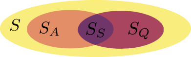
Figure 1: The set of all initial quantum states is given by $S$. Even if a quantum simulator Hamiltonian $\hat{H}_{\mathrm{QS}}$ is not the same as the target Hamiltonian $\hat{H}_{\mathrm{T}}$, there still exists some set of states $S_{Q}$ that can simulate the physics of $\hat{H}_{\mathrm{T}}$. If the overlap $S_{S}$ between the set of experimentally accessible states $S_{A}$ and $S_{Q}$ is not zero, the concept of using the connector can be used in analog quantum simulators. The same concept can be also extended to the digital version of a quantum simulator by applying quantum kicks using $\hat{H}_{\mathrm{QS}}$. The size of $S_{Q}$ depends on the form of $\hat{H}_{\mathrm{QS}}$. If $\hat{H}_{\mathrm{QS}}=\hat{H}_{\mathrm{T}}$, then $S=S_{Q}$ and $S_{A}=S_{S}$ is always a subset of $S_{Q}$.

The interpretation of $\hat{h}(t)$ is then straightforward. It is nothing else but an operator which transforms dynamics governed by $\hat{H}_{\mathrm{T}}$ to dynamics governed by $\hat{H}_{\mathrm{QS}}$. If one knows the $\hat{h}(t)$ that relates the two Hamiltonians $\hat{H}_{\mathrm{T}}$ and $\hat{H}_{\mathrm{QS}}$, it is possible to simulate dynamics generated by $\hat{H}_{\mathrm{T}}$ by $\hat{H}_{\mathrm{QS}}$ by using the transformation

$$\langle\hat{O}(t)\rangle_{\mathrm{T}}=\langle e^{-i\hat{h}(t)}\hat{O}(t)e^{i\hat{h}(t)}\rangle_{\mathrm{QS}},$$ (4)

for any observable $\hat{O}(t)$. For brevity, we will call $\hat{h}(t)$ a connector operator or simply connector. Unfortunately, due to their construction, connectors are likely to be rather complicated, time-dependent, or even non-local, and therefore most often of no practical help. However, we will show in the following that under certain conditions one can connect the dynamics governed by two substantially different Hamiltonians in a valuable way. One such condition is given in situations where two Hamiltonians commute, i.e., $\hat{h}(t)=\hat{h}\cdot t$. This means that $\hat{h}$, $\hat{H}_{\mathrm{QS}}$, and $\hat{H}_{\mathrm{T}}$ share the same eigenbasis but have different eigenspectra. Then, if $\hat{h}$ has a degenerate eigenspectrum, it might happen that a state $|\psi\rangle$ composed of degenerate eigenstates of $\hat{h}=\hat{H}_{\mathrm{QS}}-\hat{H}_{\mathrm{T}}$ will not be an eigenstate of $\hat{H}_{\mathrm{QS}}$ or $\hat{H}_{\mathrm{T}}$, but the two Hamiltonians will yield the same quantum dynamics with respect to that state (see Fig. 1). Of course, finding two different Hamiltonians that commute so that one of them can act as a quantum simulator is not easy and potentially a vast limitation. However, in the following we will discuss two interesting cases and in particular show how to make use of the knowledge of $\hat{h}(t)$ in order to simulate infinite-range interactions with a system which exhibits only short-range nearest-neighbor interactions.

Analog quantum simulators—As a first example we will consider how to simulate the well-known one-axis twisting Hamiltonian Kitagawa and Ueda (1993)

$$\hat{H}_{\mathrm{oat}}=\chi\sum_{i\leq j}^{N}\frac{\hat{\sigma}_{i}^{z}\hat{\sigma}_{j}^{z}}{4}=\chi\hat{S}_{z}^{2},$$ (5)

where $\hat{S}_{z}=\sum_{i=1}^{N}\hat{\sigma}_{i}^{z}$ is the collective spin operator. Despite its simplicity, this Hamiltonian is known to generate a wide spectrum of many-body entangled states such as spin-squeezed, twin Fock, and Greenberger-Horne-Zeilinger states if the initial state is an eigenstate of the $\hat{S}_{x}$ operator with maximal eigenvalue, i.e., $\hat{S}_{x}|\psi\rangle=N/2|\psi\rangle$ Gietka et al. (2015). It can also be realized experimentally with ultra cold gases Sørensen et al. (2001) and trapped ions Mølmer and Sørensen (1999). On the other hand, due to its formal simplicity, we can easily find a non-trivial and interesting Hamiltonian that commutes with the one-axis twisting Hamiltonian. It is straightforward to show that the Heisenberg XX model

$$\hat{H}_{\mathrm{XX}}=\frac{\beta}{4}\sum_{i=1}^{N-1}\left(\hat{\sigma}^{x}_{i}\hat{\sigma}^{x}_{i+1}+\hat{\sigma}^{y}_{i}\hat{\sigma}^{y}_{i+1}\right),$$ (6)

commutes with $\hat{H}_{\mathrm{oat}}$, and therefore any eigenstate of $\hat{H}_{\mathrm{oat}}-\hat{H}_{\mathrm{XX}}$ will give the same dynamics under the action of the two different Hamiltonians. However, as $\hat{H}_{\mathrm{oat}}-\hat{H}_{\mathrm{XX}}$ possesses a non-degenerate eigenspectrum, such a simulator is fundamentally not very interesting as it can only simulate the dynamics of eigenstates. Nevertheless, one can add an arbitrary function of $\hat{\sigma}^{z}_{i}$ to the Heisenberg XX model and it will still commute with the $\hat{H}_{\mathrm{oat}}$ since $[\hat{\sigma}_{i}^{z},\hat{H}_{\mathrm{oat}}]=0$. This then allows one to manipulate the form of $\hat{h}$ in such a way that the initial state $\hat{S}_{x}|\psi\rangle=N/2|\psi\rangle$ is also the eigenstate of $\hat{h}$, but not of the Hamiltonians building it. As an example we show that the Heisenberg XXX model with a staggered field

$$\hat{H}_{\mathrm{QS}}= \frac{\beta}{4}\sum_{i=1}^{N-1}\sum_{j\in\{x,y,z\}}\hat{\sigma}^{j}_{i}\hat{\sigma}^{j}_{i+1}+\frac{\alpha}{2}\sum_{i=1}^{N}(-1)^{i}\hat{\sigma}^{z}_{i},$$ (7)

can simulate one-axis twisting Hamiltonian in the limit $\beta\gg\alpha$ with $\alpha=\sqrt{N-1}\sqrt{\chi^{2}+\chi\beta}$ and for an even number of spins, i.e, $N=2k$ with $k\in\mathbb{N}$. Even though $\hat{H}_{\mathrm{QS}}$ and $\hat{H}_{\mathrm{oat}}$ are completely different, they realize the same dynamics. Most strikingly $\hat{H}_{\mathrm{QS}}$ contains only short-range nearest-neighbor interactions while $\hat{H}_{\mathrm{oat}}$ contains infinite-range interactions. Interestingly, we find that for an odd number of spins, $N=2k+1$, and similar conditions, i.e, $\beta\gg\alpha$ and $\alpha\approx 1.299\sqrt{N-1}\sqrt{\chi^{2}+\chi\beta}$, the Heisenberg XXX model with staggered field realizes both one-axis twisting and an effective rotation around $z$ axis with frequency given by $\alpha/N$. The rotation can be easily eliminated by moving to a frame which rotates around the $z$ axis with the same frequency but in the opposite direction, i.e., performing transformation $|\psi\rangle\rightarrow\hat{U}|\psi\rangle$ with $\hat{U}=\exp[it(\alpha\hat{S}_{z}/N)]$ (note, however, that $\hat{h}$ does not have to be proportional to $\hat{S}_{z}$). This idea is similar to moving to a frame of reference rotating with the frequency of a pumping laser, which is a typical situation in quantum optics. We can therefore identify another interesting condition for a quantum simulator using the connector. This is, even if the initial state is not an eigenstate of $\hat{h}$ but $\hat{h}$ happens to trivially transform $|\psi\rangle$ (as in the case of a collective rotation or a translation), measuring an observable in the quantum simulator allows for measuring it by performing a straightforward manipulation on the measured data, in this case given by

$$\langle\hat{S}_{x}(t)\rangle_{\mathrm{T}}=\sqrt{\langle\hat{S}_{x}(t)\rangle_{\mathrm{QS}}^{2}+\langle\hat{S}_{y}(t)\rangle^{2}_{\mathrm{QS}}}.$$ (8)

The results of the numerical simulation and calculation of $\langle\hat{S}_{x}(t)\rangle_{\mathrm{T}}$ are presented in Fig. 2.

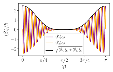
Figure 2: In order to calculate the time evolution of $\langle\hat{S}_{x}\rangle_{\mathrm{T}}$ in target system, it is necessary to measure how $\langle\hat{S}_{x}\rangle_{\mathrm{QS}}$ and $\langle\hat{S}_{y}\rangle_{\mathrm{QS}}$ depend on time in the quantum simulator system. In the numerical simulations, we have set $\chi=1$, $\beta/\alpha\approx 40.0$ ($\alpha\approx 1.299\sqrt{N-1}\sqrt{\chi^{2}+\chi\beta}$, see the main text for details), and $N=5$ spins.

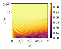
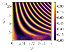
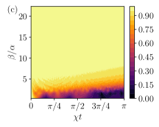
Figure 3: Fidelity between states generated by one-axis twisting [Eq. (6)] and Heisenberg spin chain [Eq. (7)] as a function of time and $\beta/\alpha$ ($\alpha\sim\sqrt{\beta}$) for a system with (a) an even number of spins ($N=6$) and (b) an odd number of spins ($N=5$). In (c) the data for the odd number of spins is re-plotted using a frame of reference rotating with frequency $\omega=\alpha/N$ around the $z$-axis. In (b) one cannot only observe one-axis twisting but also rotation of the state (due to the lack of discrete translational symmetry), which can be removed by moving to a proper frame of reference. In the numerical simulations, we have set $\chi=1$. Note that for $\chi t=\pi/2$ the state of the system is the maximally entangled Greenberger-Horne-Zeilinger state.

In order to investigate the robustness of simulating the one-axis twisting dynamics with a Heisenberg XXX chain with a staggered field, we plot the fidelity between the states generated with these two Hamiltonians for two cases $N=6$ and $N=5$ as a function of time and $\beta/\alpha$ in Fig. 3. One can see why the condition given by Eq. (1) does not require $\Im[{\xi(t)}]=0$. For times such that $\Im[{\xi(t)}]\ll 1$, the dynamics governed by the simulator still very much resembles the dynamics governed by the target Hamiltonian.

It can be also shown that Heisenberg XXX model with an arbitrary transverse field in the $z$ direction commutes with the special case of the Lipkin-Meshkov-Glick model $\hat{H}_{\mathrm{LMG}}=\hat{S}_{x}^{2}+\hat{S}_{y}^{2}+\Omega\hat{S}_{z}$ Ribeiro et al. (2007) or with $\hat{H}=\sum_{n=1}^{\infty}\gamma_{n}\hat{S}_{z}^{n}$; and the Heisenberg XXX model without a transverse field commutes with a generalized two-axis-counter twisting Hamiltonian $\hat{H}_{\mathrm{tact}}=\chi(\hat{S}_{x}\hat{S}_{y}+\hat{S}_{y}\hat{S}_{x})+\alpha\hat{S}_{x}+\beta\hat{S}_{y}+\gamma\hat{S}_{z}$. However, the question of whether one can simulate non-trivial physics of these Hamiltonians using the connector approach remains open at this time. An interesting situation arises when the two Hamiltonians do not commute. In such a case, the connector can be expressed as $\hat{h}=\sum_{n=1}^{\infty}t^{n}\hat{A}_{n}$, where $\hat{A}_{n}$ are operators that can be found according to the Baker-Campbell-Hausdorff formula. Also, when at least one of the Hamiltonians is time-dependent, it might lead to interesting possibilities of quantum simulation. All of these possibilities may relax constraints imposed on the universal analog quantum simulator, but we defer all of them to future investigations. Instead, we will focus now on the possibility of using the connector operator in the digital quantum simulator.

Digital quantum simulator—A digital quantum simulator Lloyd (1996) works by evolving a system forward using small and discrete time steps according to

$$e^{i\hat{H}_{\mathrm{T}}t}\approx\left(e^{i\hat{H}_{1}t/n}\ldots e^{i\hat{H}_{\ell}t/n}\right)^{n}.$$ (9)

By making $t/n$ small enough and using error correction protocols, this allows to simulate $\hat{H}_{\mathrm{T}}$ with an arbitrary precision.

This concept can also be applied to perform digital quantum simulation using the connector operator. If the time evolution interval is short enough, we can neglect the higher order commutators in Eq. (3), i.e.,

$$\hat{h}(t)\approx\delta t\left(\hat{H}_{\mathrm{QS}}-\hat{H}_{\mathrm{T}}\right).$$ (10)

In contrast to the situation where the Hamiltonians $\hat{H}_{\mathrm{QS}}$ and $\hat{H}_{\mathrm{T}}$ commute, here the eigenstates of $\hat{h}$ are different to the eigenstates of $\hat{H}_{\mathrm{QS}}$ and $\hat{H}_{\mathrm{T}}$. While this is in general a simplification, the price to be paid for it is that the eigenstates of $\hat{H}_{\mathrm{QS}}-\hat{H}_{\mathrm{T}}$ are only approximate eigenstates of $\hat{h}$ for short time intervals while $\frac{i(\delta t)^{2}}{2}[\hat{H}_{\mathrm{QS}},-\hat{H}_{\mathrm{T}}]\approx 0$. However, since during these the two Hamiltonians will yield the same dynamics one can perform stroboscopic dynamics by changing $\hat{H}_{\mathrm{QS}}$ to $\hat{H}_{\mathrm{QS}}^{\prime}$ after every quantum kick. If the new Hamiltonian is chosen such that the state after the last quantum kick is the eigenstate of the operator $\hat{H}_{\mathrm{QS}}^{\prime}-\hat{H}_{\mathrm{T}}$, one can then simulate $\hat{H}_{T}$ with the quantum kicks generated by $\{\hat{H}_{\mathrm{QS}},\hat{H}_{\mathrm{QS}}^{\prime},\ldots,\hat{H}_{\mathrm{QS}}^{(n)}\}$, where $n$ labels the $n$th quantum kick. Naturally, the smaller the commutator, the longer each quantum kick can be applied for, and in the limit of the commutator going to 0, we recover the analog quantum simulator discussed in the previous section. In this sense, the analog quantum simulation is a special case of digital quantum simulation where the length of the quantum kick can be infinitely long.

Similarly as in the original idea of the digital quantum simulator, the digital quantum simulator using the connector operator has to be first accordingly prepared. In the former case, one has to use the so-called Trotter expansion, and in the latter case one has to ensure that $|\psi\rangle$ is an eigenstate of $\hat{H}_{\mathrm{QS}}^{(n)}-\hat{H}_{\mathrm{T}}$ after each quantum kick. However, as the digital quantum simulator using the connector requires much fewer steps as the sequence of kicks has to applied only once instead of $n$ times [see Eq. (9)]. The price to be paid for this simplicity in relation to the standard digital quantum simulator is the fact that for every initial state, one has to come up with a unique set of quantum kicks. Nevertheless, given the fact that in the experiment only a tiny fraction of all possible quantum states can be addressed, it should not be viewed as a major obstacle (see Fig. 1). Also, depending on the particular target Hamiltonian, some quantum simulators will be better than others since some of them will minimize the commutator $[\hat{H}_{\mathrm{QS}},-\hat{H}_{\mathrm{T}}]$ allowing thus for increasing the length of a single time step $\delta t$.

Last but not least, one can think about combining the Trotter decomposition with the connector approach. Imagine that one has an operator $\hat{O}$ that commutes with the target Hamiltonian $\hat{H}_{\mathrm{T}}$ or $\hat{h}$ can be easily calculated. Then, as we have shown, for the eigenstates of $\hat{O}-\hat{H}_{\mathrm{T}}$, the unitary evolution operators $\exp({-it\hat{O}})$ and $\exp({-it\hat{H}_{\mathrm{T}}})$ will yield the same dynamics. As a consequence, if $\hat{O}$ is much simpler than $\hat{H}_{\mathrm{T}}$, decomposing $\exp({-it\hat{O}})$ should become much easier than decomposing $\exp({-it\hat{H}_{\mathrm{T}}})$.

Conclusions and outlook—By using the knowledge of a connector operator of two Hamiltonians residing in the same Hilbert space, we have proposed a way of simulating the dynamics governed by one Hamiltonian using a different one. As an example of an analog quantum simulation, we have shown how to implement the one-axis twisting Hamiltonian in the Heisenberg XXX model with a staggered field. Using the connector, we have also proposed an alternative approach to digital quantum simulators. Instead of trying to build the target Hamiltonian $\hat{H}_{\mathrm{T}}$ out of many small steps, one has to apply short quantum kicks with a quantum simulator Hamiltonian $\hat{H}_{\mathrm{QS}}$ such that after each quantum kick the state is an eigenstate of the $\hat{H}_{\mathrm{QS}}-\hat{H}_{\mathrm{T}}$ operator. This can significantly reduce the complexity of a digital quantum simulator. The price being paid is the fact that not all initial states can be easily used in the simulator (see Fig. 1). However, given the fact that not all initial states can be prepared in an experiment, by appropriately tuning the parameters of the simulator one should be able to simulate non-trivial physics of other systems. We have also identified interesting possibilities for future research including analog quantum simulation in the case when two Hamiltonians, $\hat{H}_{\mathrm{QS}}$ and $\hat{H}_{\mathrm{T}}$, do not commute or when the target Hamiltonian is time-dependent. A fascinating question that remains to be addressed in future research is whether the presented framework can be used with dissipative time evolution.

The results presented in this work might have direct implications in many branches of modern physics as well as quantum chemistry Kassal et al. (2011); Argüello-Luengo et al. (2019); McArdle et al. (2020) and quantum biology Lambert et al. (2013); Davies (2004), and can be tested in most of the current quantum simulator experimental set ups. However, the most striking consequences pave a way towards an approach to simulating dynamics not only with other systems but with other Hamiltonians. This might relax the constrains on the universal quantum simulator as it is not necessary to use exactly the same Hamiltonian to simulate the physics of some other Hamiltonians. On the downside, even though in certain situations it might be easier to perform quantum simulations exploiting the connector operator, in general it might be more challenging to find proper quantum simulators allowing for taking advantage of this framework of connector.

Additionally, we have proposed a method for creating many-body entangled states, including the spin-squeezed and the maximally entangled Greenberger-Horne-Zeilinger state, in a system exhibiting exclusively nearest-neighbor interactions. This might become extremely useful for the quantum computer architectures based on superconducting qubits as they typically exhibit only nearest or next-nearest neighbor interactions Kjaergaard et al. (2020)