The Power Spectrum Of Primordial Gravitational Waves Generated by Anisotropic Metric

Abstract

One of the predictions from simple inflation models is stochastic background of gravitational waves (or literally what is called Primordial Gravitational Waves (PGW)) with a nearly scale–invariant spectrum. To discuss a possible direct detection of PGW, the quantity so–called Spectral Energy Density (SED) has crucial role. In this work, we consider PGW amplified by inflation and generated by perturbing the Anisotropic (Bianchi type–I) metric. We focus on the SED quantity of these gravity waves. The intended frameworks are the Einstein’s and modified (pure quadratic Ricci scalar) gravities. The spectral graphs for SED shows that in Einstein’s gravity, the anisotropic model has the ability to adapt to the observational data (BBN bounds) and in the modified gravity, in addition to observational constraint adaptation, the scale–invariant character of the spectrum is much more pronounced.

Keywords: Anisotropic metric, Gravitational waves, Power spectrum, Quadratic action.

1 Introduction

One of the central predictions of Einstein’s general theory of relativity is that Gravitational Waves (GW) will be generated by accelerating masses [1, 2]. For decades, it was so difficult to analyze and to define the energy and momentum carried by GW. The first direct observation from merging massive black holes reported on September 14, 2015 [3]. This has become a renewed attention to detect new information in astronomy and cosmology. The GW are very important physical process that can be studied to give us valuable information about the dynamics of spacetime geometry and to probe in the history of the Universe. Many researches have been done in this field, among which the follows can be mentioned, e. g.  [4]–[10].
Nowadays, the sources of GW are largely known including gravitational collapse, coalescing binaries, pulsars, rapidly spinning accreting neutron stars, and the stochastic background. the Primordial Gravitational Waves (PGW)) produced in the early Universe are a type of stochastic background which emanate from regions of strong gravity. They also carry uncorrupted physical signatures of Early universe and its structure. These waves form an extremely large number of weak, independent, and unresolved sources and this makes the waves have a random character. At the present time, GW originated from inflationary period will be out of reach for all planned ground–based instruments. The detection of such a background would have a profound impact on early Universe cosmology and other research fields of physics such as High Energy physics which includes high energies events, that will never be accessible by other means.
One of the useful tools for studying and analyzing the stochastic waves is the spectral method that we apply according to its random nature, then the main reason to use the spectral method is due to the random nature of the stochastic waves. Generally, for a periodic signal, knowing the spectrum frequency and power of each harmonic contributing to the signal allows it to be decomposed into its component parts. Hence, one reconstructs the signal from its component, in which case the signal becomes more meaningful phase data. The PGW carry important information from the earliest phases of the universe and due to the various Astrophysical sources contributions, the information is disturbed. One of the important quantities in spectral methods to extract such information is the power spectrum, or more specifically in our discussion, known as Spectral Energy Density (SED) quantity $\Omega_{GW}(f)$. It is hoped that such method and tool can be of great help to provide a snapshot of the early universe. Also, It can help us to have a relative scheme of energy scale of the early universe, due to the Inflation Energy Scale is one of the main challenges in theoretical and experimental (High Energy) physics.
The study of PGW with spectral considerations in isotropic background has already been done in the works, e. g. [11, 12, 13]. Here, we do this for the case in which the background metric is an anisotropic one. The considered gravity frameworks are the Einstein’s and modify gravity, that is pure quadratic Ricci scalar ($f(R)=R^{2}$).
In the present work the emphasis on that, from spectrum of PGW perspective, the anisotropic model is compatible with the observations as isotropic model (In the other words in the case of anisotropic background, the spectrum of PGW have the ability to adapt to the observational constraints (as isotropic background), that is, in line with LIGO S5 (known as Big–Bang–Nucleosynthesis (BBN) Bounds)[14, 15]. In the other words, we study and analyze PGW produced by tensor perturbations amplified by inflation in the early stage of th universe. For this purpose, we consider an anisotropic (Bianchi type–I) background metric and the evolution equations for perturbations are presented in the Einstein’s and modified gravities. Finally, the graph of spectrums for the perturbations along with the corresponding spectrum graph in the isotropic universe are illustrated. In Einstein’s gravity, a comparison of the graphs shows, in the anisotropic case as isotropic one, the BBN bound is adapted. In modified gravity, in addition to observational adaptation, the Scale–Invariant character of spectrum is remarkable. Interestingly, up to now the authors have done the calculations, have found no perturbation solutions in the isotropic case and consequently no spectrum.
Our approach to obtain evolution equations is the Lagrangian method. As we will see, in Einstein’s framework to obtain evolution equations, using the scale factor instead of conformal–time would be a good trick to avoid the piece–wise function. The use of the piece–wise function and study from another in point of views can be found in e. g. [19, 20, 21, 22, 23]. The work is organized as follows: In section II, we introduce the motion equations of tensor perturbations essential for the work. In section III, the power spectrum of perturbations in Einstein’s and modified frameworks is investigated. The conclusions are given in section IV.

2 Evolution Equations

In this section, we introduce the equations of motion for the (tensorial) perturbations of the anisotropic (Bianchi type–I) background metric $\bar{g}_{\mu\nu}$ given by

$$ds^{2}=\bar{g}_{\mu\nu}dx^{\mu}dx^{\nu}=-dt^{2}+A^{2}dx^{2}+B^{2}dy^{2}-C^{2}dz^{2},$$ (1)

where $A,B,C$ are the directional scale factors with $A=B=C=a(t)$. Suppose this spacetime is perturbed and the line element (1) changes as follows

$$ds^{\prime 2}=g_{\mu\nu}dx^{\mu}dx^{\nu}=\left(\bar{g}_{\mu\nu}+h_{\mu\nu}\right)dx^{\mu}dx^{\nu}=a^{2}\left(-d\tau^{2}+dx^{2}+dy^{2}-dz^{2}\right)+a^{2}h_{ij}dx^{i}dx^{j},$$ (2)

where $\tau$ is conformal time and $h_{ij}=h_{ij}(\tau,\textbf{x})$ are the perturbations satisfying, symmetric ($h_{ij}$=$h_{ji}$), traceless ($h^{i}_{i}=0)$ and transverse $(h^{j}_{i,j}=0)$ conditions.
The equations of motion for perturbations, in a general $f(R)$ gravity, are obtained by variation of the following action

$$S=\int d\tau d\textbf{x}\sqrt{-\bar{g}}\left(f(R)+\frac{1}{2}\Pi_{ij}h_{ij}\right),$$ (3)

where $\Pi_{ij}$ is the anisotropic stress tensor[24]. For the isotropic perturbations (that is $h_{ij}(\tau,x,y,z)=h(\tau,x,y,z)=h(\tau,\textbf{x})$) and the vacuum or perfect fluid ($\Pi_{ij}=0$) cases, the equations of motion take the following form [25]

$$\partial_{\mu}\left(\sqrt{|\bar{g}|}\hskip 2.84526ptf^{\prime}(R)\hskip 2.84526pt\frac{\partial R}{\partial(\partial_{\mu}h)}\right)=0,$$ (4)

where the Ricci scalar corresponding to perturbed metric (2) is given by [12]

$$R=-\frac{\bar{g}^{\mu\nu}}{64\pi G}\left(\partial_{\mu}h\partial_{\nu}h\right)=\frac{a^{-2}}{64\pi G}\left(h^{{}^{\prime}2}-(\partial_{x}h)^{2}-(\partial_{y}h)^{2}+(\partial_{z}h)^{2}\right),$$ (5)

where the prime is derivative with respect to conformal time, namely (${}^{\hskip 2.84526pt{}^{\prime}}\equiv\frac{\partial}{\partial\tau}$).
We treat the motion equation (4) for the two cases of $f(R)=R$ and $R^{2}$, which by substituting them into (4) we get, respectively

$$\partial_{\mu}\left(\sqrt{|\bar{g}|}\hskip 2.84526pt\hskip 2.84526pt\bar{g}^{\mu\nu}\partial_{\nu}h\right)=0,$$ (6)

$$\partial_{\mu}\left(\sqrt{|\bar{g}|}\hskip 2.84526ptR\hskip 2.84526pt\bar{g}^{\mu\nu}\partial_{\nu}h\right)=0.$$ (7)

In the next section, we use the latter equations to obtain the evolution of perturbations and consequently their spectrum.

3 The Power Spectrum

In this section, we first write down the motion equations for the primordial tensorial perturbations leading to the PGW in the Einstein’s and pure quadratic gravities. The background metric for the perturbations is anisotropic Bianchi type–I one. Then, the corresponding spectrums of perturbations are presented.

3.1 Spectrum in Einstein Gravity

By substituting the anisotropic background metric (2) into the equation (6), the evolution equation for the metric perturbations reads

$$h^{{}^{\prime\prime}}+2\left(\frac{a^{{}^{\prime}}}{a}\right)h^{{}^{\prime}}-\left(\partial_{x}^{2}+\partial_{y}^{2}-\partial_{z}^{2}\right)h=0.$$ (8)

This equation differs from the isotropic case only by the minus sign of the last term (namely $-\partial_{z}^{2}$) [11, 12]. Note that in equation (8), $h=h(\tau,\textbf{x})$ and prime is derivative respect to $\tau$, and we need to Fourier transform to calculate the SED. For abbreviation, we denote the Fourier transform of $h(\tau,\textbf{x})$ by $h(\tau,\textbf{k})$, then by taking Fourier transforms of both sides (8), one gets

$$h^{\prime\prime}(\tau,\textbf{k})+2\left(\frac{a^{{}^{\prime}}}{a}\right)h^{\prime}(\tau,\textbf{k})+\left(k_{x}^{2}+k_{y}^{2}-k_{z}^{2}\right)h(\tau,\textbf{k})=0.$$ (9)

The conventional method for solving the equation (9) is to first specify the scale factor (as a function of time) for each cosmological period to find the corresponding solution and finally matching the solutions at the epoch of the transition between the periods (see e. g. [11, 12]). Here, we will use the method of uniformity of the equation instead, meaning that, we replace the time derivatives with the derivatives respect to the scale factor. This is done through the familiar relation $dt=ad\tau$ which allows perturbations to be expressed on scale factor rather than the conformal time, that is $h(\tau,\textbf{x})\rightarrow h(a,\textbf{x})$ (or equivalently $h(\tau,\textbf{k})\rightarrow h(a,\textbf{k})$). Therefore, equation 9 will have the following (uniform) form [25]:

$$a^{4}H^{2}h_{aa}(a,k)+\left(4a^{3}H^{2}+\frac{a^{4}}{2}\frac{dH^{2}}{da}\right)h_{a}(a,k)+\left(k_{x}^{2}+k_{y}^{2}-k_{z}^{2}\right)h(a,k)=0,$$ (10)

where $h_{a}(a,k)=\frac{dh(a,k)}{da}$ , $h_{aa}(a,k)=\frac{d^{2}h(a,k)}{da^{2}}$ and $H=\frac{\dot{a}}{a}=h^{\prime}/h_{a}$. Now, knowing the Hubble parameter as a function of scale factor $H=H(a)$, equation (10) becomes uniform, meaning that it consists of only one dependent variable $a$ and one independent variable $h(a,k)$. It is not difficult to show that here the Hubble parameter has the same form in the isotropic case, that is

$$H^{2}(a)=H^{2}_{0}\left(\Omega_{r}a^{-4}+\Omega_{m}a^{-3}+\Omega_{\Lambda}\right),$$ (11)

where $\Omega_{r}=9.4\times 10^{-5}\simeq 10^{-4}$, $\Omega_{m}=0.3$, and $\Omega_{\Lambda}=0.7$ are radiation, matter and dark energy density parameters, respectively.
As we see below, to calculate SED, we need to the solution to the equation (10) and for this purpose, we will now introduce the relevant quantities. The first is the spectral amplitude $\Delta_{h}^{2}(\tau,k)$ defined by

$$<h_{ij}(\tau,\textbf{x})h^{ij}(\tau,\textbf{x})>=\int\frac{dk}{k}\Delta_{h}^{2}(\tau,k),$$ (12)

which can be written in the reverse form as

$$\Delta_{h}^{2}(\tau,k)=\frac{k^{3}}{\pi^{2}}<|h(\tau,k)|^{2}>,$$ (13)

or, in terms of scale factor

$$\Delta_{h}^{2}(a,k)=\frac{k^{3}}{\pi^{2}}<|h(a,k)|^{2}>.$$ (14)

This amplitude relates the spectral distribution of the amplified fluctuations and the cosmological kinematic parameters. It is also useful to describe the distribution of the modes in outside the horizon.
The second quantity is the same SED which characterizes the intensity of a stochastic GW background and is given by

$$\Omega_{h}(a,k)=\frac{1}{\rho_{c}}\frac{d\rho}{d\ln k},$$ (15)

where $\rho$ and $\rho_{c}$ are energy density and critical energy density, respectively. Since, the relic GW with mode inside horizon should be still present today, they must be accessible to direct observations. The SED characterises the spectrum of the relic waves and thus it is useful to discuss a possible their direct detection. For the mode inside horizon, the spectral energy density is related to the spectral amplitude through the relation

$$\Omega_{h}(a,k)=k^{2}\frac{\Delta_{h}^{2}}{12\hskip 1.42262pta^{2}H^{2}(a)}=\frac{k^{5}}{12\pi^{2}}\frac{<|h(a,k)|^{2}>}{\hskip 1.42262pta^{2}H^{2}(a)}.$$ (16)

The spectrum of waves at the present time $\tau_{0}$ is obtained by substituting the conventional value of scale factor ($a(\tau_{0})=a_{0}=1$) into (16) which gives

$$\Omega(k)=\Omega_{h}(1,k)=\frac{k^{5}}{12\pi^{2}}\frac{<|h(1,k)|^{2}>}{\hskip 1.42262ptH_{0}^{2}}=\frac{k^{5}}{3\pi^{2}}\frac{|h(k)|^{2}}{\hskip 1.42262ptH_{0}^{2}},$$ (17)

where we have used $|h(k)|^{2}=\frac{1}{2}\left(\langle|h_{+}|^{2}\rangle+\langle|h_{\times}|^{2}\rangle\right)=\frac{1}{4}\langle h^{ij}h_{ij}\rangle=\frac{1}{4}<|h(1,k)|^{2}>$.
Equation (16) or (17) represents form of the spectrum dependence on the perturbations which must be determined from equation (10)and this in turn requires the appropriate initial conditions. Knowing that PGW are originated from inflationary period, the appropriate initial conditions can be considered as

$$h\left(a_{e},k\right)=1$$ (18)

$$\hskip 4.2679pth_{a}\left(a_{e},k\right)=0,$$

where $a_{e}\simeq 10^{-27}$ is the scale factor at the end of inflation [26]. By having the initial conditions and determining the Hubble function in equation (10), we can calculate the evolution of perturbation and from there compute the SED. The process of such computations are performed using numerical instructions and the results are shown in Figure 1 and 2. The computations are done in the following two cases of the Hubble rate (11):
1) Matter dominate, that is $H(a)\approx H_{0}\sqrt{\Omega_{m}a^{-3}}$.
2) Matter–Dark energy dominate, that is $H(a)\approx H_{0}\sqrt{\Omega_{m}a^{-3}+\Omega_{\Lambda}}$.
It should be noted, the general case $H(a)=H_{0}\sqrt{\Omega_{r}a^{-4}+\Omega_{m}a^{-3}+\Omega_{\Lambda}}$, hasn’t much different from the two above cases, due to insignificant contribution of the radiation term ($\Omega_{r}\simeq 10^{-4}$).
The following descriptions can be helpful to get more the figures:
1) Fig.1 shows the graph of the spectrum for isotropic and anisotropic universes in Matter dominate case, that is $H(a)\approx H_{0}\sqrt{\Omega_{m}a^{-3}}=H_{0}\sqrt{0.3a^{-3}}$ . The orange graph corresponds to isotropic universe and the two other graphs correspond to anisotropic universe with two different wave vectors, namely, the blue graph for $\vec{\textbf{k}}=\frac{k}{\sqrt{3}}\textbf{i}+\frac{k}{\sqrt{3}}\textbf{j}+\frac{k}{\sqrt{3}}\textbf{k}$, and yellow graph for $\vec{\textbf{k}}=\sqrt{\frac{2}{5}}k\hskip 1.42262pt\textbf{i}+\sqrt{\frac{2}{5}}k\hskip 1.42262pt\textbf{j}+\sqrt{\frac{1}{5}}k\hskip 1.42262pt\textbf{k}$.
2) Fig.2 shows the graph of the spectrum for isotropic and anisotropic universes in Matter–Dark energy dominate case, that is $H(a)\approx H_{0}\sqrt{\Omega_{m}a^{-3}+\Omega_{\Lambda}}=H_{0}\sqrt{0.3a^{-3}+0.7}$. The red graph corresponds to isotropic universe and the two other graphs correspond to anisotropic universe with two different wave vectors, namely the blend graph for $\vec{\textbf{k}}=\frac{k}{\sqrt{3}}\textbf{i}+\frac{k}{\sqrt{3}}\textbf{j}+\frac{k}{\sqrt{3}}\textbf{k}$, and yellow graph for $\vec{\textbf{k}}=\sqrt{\frac{2}{5}}k\hskip 1.42262pt\textbf{i}+\sqrt{\frac{2}{5}}k\hskip 1.42262pt\textbf{j}+\sqrt{\frac{1}{5}}k\hskip 1.42262pt\textbf{k}$.
As can be seen from the figures, the graph spectrums in anisotropic universe, like in the isotropic state [25], has the ability to adapt to observations bounds BBN. The BBN calculations puts an upper limit for SED, such that ($\Omega_{GW}(f)\leq 6.9\times 10^{-6}$ around $f\sim 100Hz$ or $k=\frac{2\pi f}{c}\simeq 628\hskip 1.42262ptm^{-1}$, in $c=1$ unity [14, 15]).

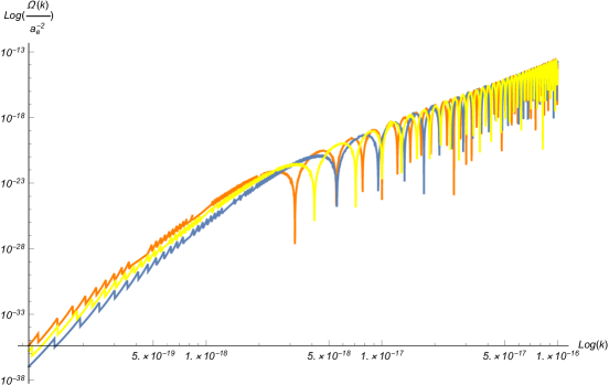
Figure 1: The power spectrum in isotropic (orange) and anisotropic (blue for $\vec{\textbf{k}}=\frac{k}{\sqrt{3}}\textbf{i}+\frac{k}{\sqrt{3}}\textbf{j}+\frac{k}{\sqrt{3}}\textbf{k}$, and yellow for $\vec{\textbf{k}}=\sqrt{\frac{2}{5}}k\hskip 1.42262pt\textbf{i}+\sqrt{\frac{2}{5}}k\hskip 1.42262pt\textbf{j}+\sqrt{\frac{1}{5}}k\hskip 1.42262pt\textbf{k}$) cases for $H(a)\approx H_{0}\sqrt{\Omega_{m}a^{-3}}$.

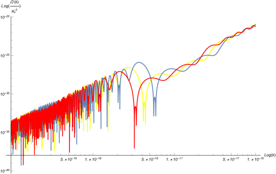
Figure 2: The power spectrum in isotropic (red) and anisotropic (blend for $\vec{\textbf{k}}=\frac{k}{\sqrt{3}}\textbf{i}+\frac{k}{\sqrt{3}}\textbf{j}+\frac{k}{\sqrt{3}}\textbf{k}$, and yellow for $\vec{\textbf{k}}=\sqrt{\frac{2}{5}}k\hskip 1.42262pt\textbf{i}+\sqrt{\frac{2}{5}}k\hskip 1.42262pt\textbf{j}+\sqrt{\frac{1}{5}}k\hskip 1.42262pt\textbf{k}$) cases for $H(a)\approx H_{0}\sqrt{\Omega_{m}a^{-3}+\Omega_{\Lambda}}$.

3.2 Spectrum in Modified Gravity $f(R)=R^{2}$

In this section, the spectrum diagrams corresponding to primordial (tensor) perturbations of anisotropic background are presented in the modified gravity framework. To begin this, we substitute background metric (2) and Ricci scalar (5) in equation (7) to obtain

$$\partial_{\tau}(S\hskip 2.84526pth^{{}^{\prime}})-\partial_{x}\left(S\hskip 2.84526pt\partial_{x}h\right)-\partial_{y}\left(S\hskip 2.84526pt\partial_{y}h\right)+\partial_{z}\left(S\hskip 2.84526pt\partial_{z}h\right)=0,$$ (19)

where $S=h^{{}^{\prime}2}-(\partial_{x}h)^{2}-(\partial_{y}h)^{2}+(\partial_{z}h)^{2}$. Equation (19) is the Modified Gravity counterpart of equation (8) in Einstein’s Gravity. It is a nonlinear equation and as we know for these equations, the variety of solutions can be more than the linear one. For example, equation (19) can have the following typical solutions:

$$h(\tau,\textbf{x})=A\left\{\begin{array}[]{lr}\cos(x+y-z-\tau)\pm e^{-\left|x+y-z-\tau\right|},&\\ \cos(\tau-x-y-z)\pm e^{-|\tau-x-y-z|},&\\ \sin(\tau-x-y-z)\pm e^{-|\tau-x-y-z|},&\\ \cos(\tau-x-y-z)\pm\sin(\tau-x-y-z),\end{array}\right.$$

where $A$ is a constant. Note that the variety allows to choose the solutions that are more in line with physical conditions. In order to compute the power spectrum, we choose the followings:

$$h_{1}(\tau,\textbf{x})=A\left[\cos(x+y-z-\tau)-e^{-\left|x+y-z-\tau\right|}\right]$$ (20)

and

$$h_{2}(\tau,\textbf{x})=A\left[\sin(\tau-x-y-z)+e^{-|\tau-x-y-z|}\right],$$ (21)

where as we see below, the latter solution can’nt satisfy the observational bounds and hence it isn’t acceptable.
Fourier transform is required to calculate the spectrum which is defined by:

$h(\tau,\textbf{k})=\frac{1}{(2\pi)^{3}}\int\sqrt{|\bar{g}|}d\textbf{x}e^{-i\textbf{k.x}}h(\tau,\textbf{x}),$

where there is a delicate point about limits in calculating the above Fourier integral. This means that it is true that the limits of the integral are from negative infinity to positive ones, but for our real physical space, these limits can be replaced by the Hubble radius, that is $R_{H}=(a_{0}H_{0})^{-1}$. By applying Hubble limits and considering the wave vector as $\vec{\textbf{k}}=\frac{k}{\sqrt{3}}\textbf{i}+\frac{k}{\sqrt{3}}\textbf{j}+\frac{k}{\sqrt{3}}\textbf{k}$, the spectral energy density corresponding to equation (17) for both solutions can be obtained as follows:

$$\Omega_{1}(k)=\frac{k^{5}}{3\pi^{2}}\frac{|h_{1}(k)|^{2}}{\hskip 1.42262ptH_{0}^{2}}=\frac{27\hskip 1.13809ptk\hskip 1.13809ptO}{192\hskip 2.84526pt}\sin^{4}(\frac{2\hskip 2.84526ptkR_{H}}{\sqrt{3}})\left[\left(P^{3}\cos\tau-PQ^{2}\cos\tau-\frac{2}{\pi^{3}}\frac{\sqrt{3}}{3+k^{2}}\right)^{2}-Q^{2}\sin^{2}\tau\left(Q^{2}-P^{2}\right)^{2}\right]$$ (22)

and

$$\Omega_{2}(k)=\frac{k^{5}}{3\pi^{2}}\frac{|h_{2}(k)|^{2}}{\hskip 1.42262ptH_{0}^{2}}=-\frac{k^{5}R_{H}^{4}\hskip 0.85358ptO}{64}\left[Q^{2}\cos^{2}\tau(Q^{2}+3P^{2})^{2}-\left(P^{3}\sin\tau+3Q^{2}P\sin\tau+\frac{2}{\pi^{3}}\frac{\sqrt{3}}{3+k^{2}}\right)^{2}\right]$$ (23)

where, $O=\frac{A^{2}a^{8}}{H_{0}^{2}\pi^{2}}$ , $P=\delta(\frac{k}{\sqrt{3}}-1)+\delta(\frac{k}{\sqrt{3}}+1)$ and $Q=\delta(\frac{k}{\sqrt{3}}-1)-\delta(\frac{k}{\sqrt{3}}+1)$.
The corresponding spectrum graphs (using the numerical recipes) will be in the form of Figure 3, this figure contains two graphs which the red graph shows the spectrum corresponds to the perturbation solution (20) and blue graph shows the spectrum corresponds to the perturbation solution (21). As it can be seen easily, the blue graph hasn’t a proper physical meaning, on the one hand due to the stochastic nature of the perturbations and on the other hand because of the BBN bounds. Contrary to the blue graph, the red graph acceptable conditions. The noteworthy thing about the red graph is that while it satisfies the BBN bounds, it also has the slight (negligible) slop to evoke the nearly Scale Invariant character of the spectrum predicted by Inflation models.

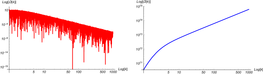
Figure 3: The graphs spectrums corresponding to the perturbations, $h_{1}(\tau,\textbf{x})$ (red) and $h_{2}(\tau,\textbf{x})$ (blue) in anisotropic universe. In the calculations, numerical value of the constant is $A=10^{-16}.$

4 Conclusions

The power spectrum corresponding to the primordial metric perturbations (leads to PGW) arisen from anisotropic background (Bianchi type–I metric) are presented in the Einstein’s and modified gravities (pure quadratic Ricci scalar). The main conclusions are summarized as follows:
1) In Einstein’s gravity, it is found that in the anisotropic model (like the isotropic one) the spectral graphs corresponding to perturbation solutions and have the ability to adapt to BBN data.
2) In modified gravity, the diversity of the perturbation solutions allows the corresponding spectral diagrams, not only match with the BBN data, but also have the scale–invariant character predicted by the inflation models.
Declarations
My manuscript has no associated data.

References

- [1] A. Einstein, Sitzungsber. Preuss. Akad. Wiss. Berlin, Math. Phys, 688-696 (1916).
- [2] A. Einstein, Sitzungsber. Preuss. Akad. Wiss. Berlin, Math. Phys, 154-167 (1918).
- [3] B.P. Abbott and R. Abbott et al., Phys. Rev. Lett. 116, 061102 (2016).
- [4] B.P. Abbott and R. Abbott et al., Phys. Rev. Lett. 116, 241103 (2016).
- [5] B.P. Abbott and R. Abbott et al., Phys. Rev. Lett. 118, 221101 (2017).
- [6] B.P. Abbott and R. Abbott et al., Phys. Rev. Lett. 119, 141101 (2017).
- [7] B.P. Abbott and R. Abbott et al., The Astrophysical Journal Letters, 851:L35 (2017).
- [8] B.P. Abbott and R. Abbott et al., Phys. Rev. Lett. 119, 161101 (2017).
- [9] N. Yunes and X. Siemens. Living Rev. Relativity, 16, 9 (2013).
- [10] M. Vallisneri, Phys. Rev. D 86, 082001 (2012).
- [11] Y. Watanabe. E. Komatsu, Phys. Rev. D 73, 123515 (2006).
- [12] L. A. Boyle and P. J. Steinhardt, Phys. Rev. D 77, 063504 (2008).
- [13] R. Jinno,T. Moroi and K. Nakayama, JCAP 01(2014)040.
- [14] B. P. Abbott et al. (LIGO Scientific Collaboration and Virgo Collaboration), Nature (London) 460, 990(2009).
- [15] W. Zhao, Phys. Rev. D 83, 104021(2011).
- [16] S. M. Carroll, V. Duvvuri, M. Trodden, M. S. Turner, Phys. Rev. D 70, 043528 (2004).
- [17] J. Naf, P. Jetzer, Phys. Rev. D 84 024027 (2011).
- [18] T. P. Sotiriou, V. Faraoni, Rev. Mod. Phys. 82, 451 (2010).
- [19] H. T. Cho and A. D. Speliotopoulos, Phys. Rev. D 52, 5445-5458 (1995).
- [20] B. Saha and G.N. Shikin, arXiv:gr-qc/0102059 1.
- [21] S. Datta and S. Guha, arXiv:gr-qc/1908.06743 1.
- [22] M. Sharma and S. Sharma, The African Review of Physics 11, 0039(2016).
- [23] A. H. Hasmani and Ahmed M. Al-Haysah, Applications and Applied Mathematics: An International Journal (AAM) 14, 334 (2019).
- [24] S. Weinberg, Phys. Rev. D 69, 023503 (2004).
- [25] T. Mohammadi, B. Malekolkalami and X. Ghamari, International Journal of Theoretical Physics 61, 15 (2022).
- [26] S. Dodelson and F. Schmidt, Modern Cosmology, ACADEMIC PRESS, p.162, (2021).