GeoStat Representations of Time Series for Fast Classification

Abstract

Recent advances in time series classification have largely focused on methods that either employ deep learning or utilize other machine learning models for feature extraction. Though successful, their power often comes at the requirement of computational complexity. In this paper, we introduce GeoStat representations for time series. GeoStat representations are based off of a generalization of recent methods for trajectory classification, and summarize the information of a time series in terms of comprehensive statistics of (possibly windowed) distributions of easy to compute differential geometric quantities, requiring no dynamic time warping. The features used are intuitive and require minimal parameter tuning. We perform an exhaustive evaluation of GeoStat on a number of real datasets, showing that simple KNN and SVM classifiers trained on these representations exhibit surprising performance relative to modern single model methods requiring significant computational power, achieving state of the art results in many cases. In particular, we show that this methodology achieves good performance on a challenging dataset involving the classification of fishing vessels, where our methods achieve good performance relative to the state of the art despite only having access to approximately two percent of the dataset used in training and evaluating this state of the art.

1 Introduction

Time series analysis has long been an important focus of quantitative research, largely due to the ubiquitous presence of time series data in a wide variety of applications such as finance, kumar2002clustering ; taylor2008modelling , medicine wismuller2002cluster , illegal fishing kroodsma2018tracking ; boerder2018global , among others, too many to list here. Contemporary work has focused on utilizing increased computational abilities to move past ARIMA models box2015time that, though expressive, heavily depend on certain assumptions that may not hold in practice.

Our focus is time series classification. This subfield has a rich body of work on methodology, and a (relative to other fields) large body of work on testing said methodology, with researchers taking care to validate results in order to determine the state of progress in said field bagnall2017great . State of the art methods contemporary to this work primarily consist of ensemble methods baydogan2013bag ; bagnall2015time ; lines2016hive ; schafer2017fast ; fawaz2019inceptiontime ; shifaz2020ts . These methods combine simpler classifiers, such as those based on distances berndt1994using , shapelets ye2009time ; hills2014classification , coefficients of autoregressive models corduas2008time , and other features to develop methods that play off the successes and weaknesses of both the features and simpler classifiers. Though accurate, ensemble models can require significant computational resources. TS-CHIEF, one such model, was shown to require multiple days of training in order to evaluate performance on the UCR/UEA 2015 Archive ucr2018website ; dau2019ucr ; this is still a significantly shorter runtime than HIVE-COTE shifaz2020ts .

Outside of ensemble models, researchers developing novel classification methods have primarily turned to deep learning based methods, playing off of its success in other fields cui2016multi ; le2016data ; wang2017time ; zhao2017convolutional ; ma2019learning . Many of these methods were analyzed in fawaz2019deep , where it was observed that some of them (in particular, ResNet he2016deep ) performed extremely well relative to ensemble models. Furthermore, the authors showed empirically that class activation maps zhou2016learning ; song2020representation could be used in tandem with networks to identify influential regions used in making a particular classification decision. Deep learning classifiers are generally less computationally intensive to train than ensemble models, but still require a fair amount of time: it took approximately 100 GPU days in order to train each of the nine models used in he2016deep a total of ten times each.

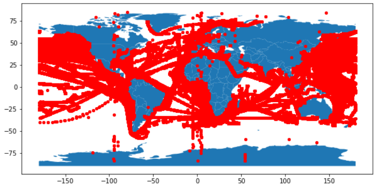
Figure 1: Spatial range of one hundred vessels in the Global Fishing Watch dataset GFWData . Red indicates a coordinate reached by one of the vessels. Note that there are some obvious errors, e.g. some vessels have coordinates on land.

Regardless of the exact type of proposed method, one method remains at the foundation of time series classification: nearest-neighbor Euclidean distance after dynamic time warping (NN-DTW) jeong2011weighted ; bagnall2014experimental ; bagnall2017great . Highly regarded for its simplicity and ease of implementation, it has long been the baseline to which any novel time series classifier should be compared. Using this classifier as a baseline makes a seemingly innocent but crucial assumption on a given dataset: Euclidean distance after dynamic time warping is a meaningful way to separate time series. Perhaps surprisingly to some readers, this is not always the case. A meaningful real-world counterexample to this idea can be found within a publicly available dataset of naval vessel trajectories over the course of four years provided by Global Fishing Watch GFWData ; GFWWebsite The trajectories within this dataset consist of twelve separate classes, each of which is a distinct type of vessel. Vessels of the same class can be on extremely different regions of the Earth, suggesting that Euclidean (or any spatial) distance is not a reasonable metric. Further, vessels can have highly different patterns of activity (both in terms of time of movement as well as type of movement), suggesting that dynamic time warping itself may not be meaningful. We defer further dataset details to later sections, but to illustrate the complexity of the problem, we show in Figure 1 the spatial range of one hundred trajectories, less than a tenth of those present in the dataset.

Nevertheless, as vessels of the same class do not necessarily correspond to the same region, NN-DTW is not a reasonable classifier to use. The best known classification model for this particular problem is a convolutional neural network with millions of parameters kroodsma2018tracking , but this model was trained and tested on a large amount of commercial data not publicly available; the data available in GFWData ; GFWWebsite is less than two percent of that used in kroodsma2018tracking . It is natural to ask, especially given the relatively limited size of the publicly available portion of the data, if a simpler model could still do reasonably well.

In light of the above, there are two questions motivating this paper. First, given the preceding paragraph, we ask whether it is possible to develop a simple model for time series classification that does not require the use of distances between individual points or dynamic time warping. Such a model would allow for a straightforward baseline to benchmark other newly proposed methods with fewer assumptions on the underlying data. Second, we wish to investigate a question stemming from an interesting point made in he2016deep . Many in the time series classification community have seemingly ignored whether such problems could be solved by pure feature learning algorithms. This was partially addressed in lubba2019catch22 , which showed it was possible to learn a small number of features that yielded good classification performance on a large number of datasets. We take this one step further by asking whether easy to compute, mathematically well-understood features exist, without employing any specific algorithm for learning them. We answer both questions we posed in the affirmative, with a surprising twist: all features we use arise from differential geometry.

In this paper, we propose the GeoStat representation for time series data in terms of summary statistics of distributions of well-understood differential geometric features, ignoring many oft-used quantities in time series analysis (e.g. autocorrelation and Fourier transforms). All quantities used are simple to compute in both univariate and multivariate settings, and only require assuming mild smoothness of the time series of interest, which can be easily achieved via standard smoothing methods. We show through extensive empirical evaluation that using (potentially multi-windowed versions of) this representation to train standard $k$NN and SVM classifiers hastie2009elements results in surprisingly good classification rates. Specifically, these classifiers have performance that is generally competitive with deep learning methods, and often state of the art; this methodology is, to the best of our knowledge, is the first to achieve perfect classification rates on average for a number of datasets in the oft-used UCR Time Series Classification Archive benchmark ucr2018website ; dau2019ucr . Our goal, however, is not to claim that our methodology is state of the art: in many cases, it is not. Rather, our goal is to illustrate that this method yields a powerful baseline for time series classification, suggesting that the representation proposed here could be used in more sophisticated methods (e.g. deep learning and ensemble methods) for working with time series.

The paper is outlined as follows. In Section 2 preliminaries and prior work related to our paper. In Section 3, we detail the general pipeline to obtain features and statistics needed we use for classification. In Section 4, we present results on both the aforementioned vessel trajectory problem as well as on the UCR 2018 archive dau2019ucr , demonstrating the effectiveness of our representation and proposed baseline. In Section 5, we evaluate the role of different parameters and features used, showing in part that in many cases we can accurately classify time series using the proposed representation on specific windows in time. We finish with concluding remarks. Additional experiments and details that do not fit within the page constraints will be deferred to the Appendix.

2 Preliminaries

2.1 Definitions and Notation

A general (finite) time series is a sequence of points ${\bf{x}}=\{x_{t_{k}}\}_{k=0}^{n}.$ We assume that $x_{t_{k}}$ is a point in $d$-dimensional Euclidean space. Though not all time series we work with are equally spaced in time, i.e. $t_{k+1}-t_{k}$ is not necessarily constant in $k,$ our methods will require this, which can easily be achieved via interpolation. We will specifically use linear interpolation: the linear interpolant $F_{\bf{x}}(t)$ of $\bf{x}$ is defined by, for $t_{0}\leq t_{i}\leq t\leq t_{i+1}\leq t_{n},$

$$F_{\bf{x}}(t)=\frac{t-t_{i}}{t_{i+1}-t_{i}}x_{t_{i}}+\frac{t-t_{i+1}}{t_{i+1}-t_{i}}x_{t_{i+1}}.$$ (1)

Our use of linear interpolation is deliberate: it ensures that time series of physical quantities are still physically meaningful (e.g. interpolants of positive quantities remain positive).

Without further assumptions on $\bf{x},$ it is possible that the interpolated time series will have sharp changes. Many of the quantities of interest for the representation we define in Section 3 require computing derivatives, which do not behave well with sharp changes. To get around this, we employ a simple smoothing operation. Namely, given a time series $\bf{x},$ we define the Laplacian smoothing operation $L$ by
$L(\bf{x})=\bf{\tilde{x}},$ where ${\bf{\tilde{x}}}=\{\tilde{x}_{t_{k}}\}_{k=0}^{n}$ is the time series defined by $\tilde{x}_{t_{0}}=x_{t_{0}},\tilde{x}_{t_{n}}=x_{t_{n}},$ and for $1\leq k\leq n-1,$

$$\tilde{x}_{t_{k}}=\frac{1}{2}(x_{t_{k+1}}-x_{t_{k}})+\frac{1}{2}(x_{t_{k-1}}-x_{t_{k}}).$$ (2)

Given a time series $\bf{x},$ we will denote by $\bf{\dot{x}}$ and $\bf{\ddot{x}}$ its first and second time derivatives. Our choice is motivated by its compactness and is commonly used in applications involving time derivatives. All derivatives computed are via the usual finite difference numerical approximation.

2.2 Related Work

We briefly review the most relevant works to us and otherwise defer the reader to excellent review articles already published: see aghabozorgi2015time ; bagnall2017great ; fawaz2019deep for general overviews. Also, please see mazimpaka2016trajectory ; bian2019trajectory for trajectory methods.

Analogues of some the specific features we use in our method have been studied within the time series classification literature. In particular, a number of single-model classifiers of interest depend on the extraction of summary features of the behavior of a time series on a given subinterval, sometimes called interval features rodriguez2004support ; deng2013time . One particular type of interval features of interest, shapelets, are subsequences of given time series that are chosen based on their perceived importance in determining the label of a given time series ye2009time ; hills2014classification . Though interval features are natural to consider, they lead to a difficult question of determining which subintervals are most representative of a given class. This is a computationally expensive but necessary question in order to deal with both computational and memory limitations. We avoid these issues by using features that are determined locally around a given time sample, which neither requires a subinterval search nor an extensive amount of memory.

Unsurprisingly, we are not the first to propose a general summary representation for time series. Of recent note is lubba2019catch22 , in which the authors showed that accurate time series classifiers could be constructed from 22 features that were learned a pool of 4791 possibilities. Our work is distinct in multiple ways: our proposed representation is of fairly higher dimension, does not need to be learned, and is derived only from differential geometric quantities. Perhaps the closest papers to ours in methodology stem from works focused on trajectory classification zhang2009learning ; etemad2018predicting . Specifically, in etemad2018predicting , the authors extract a number of features from each time point sampled from a given trajectory. These features are then used to compile distributions of each feature that was observed over time. Next, these distributions are summarized by a number of statistics, many of which we employ. The crucial difference in our work is the simultaneous increase the mathematical rigor of their treatment of bearing (the direction in which a trajectory is moving), which is incompatible with quantities of interest from differential geometry. Moreover, our approach is more general and can be applied to time series for which the analogous information is not immediately given. Finally, we propose the use of additional statistical quantities of interest which have nontrivial roles in establishing the accuracy of a classifier based on our presented experiments.

3 Representing Time Series Through Geometry

3.1 Review of Differential Geometry for Curves

As our representation fundamentally relies of differential geometry (and thus, the existence of derivatives), we make the following crucial assumption: every time series ${\bf{x}}$ of interest is a (sufficiently dense) approximation of a twice continuously differentiable ($C^{2}$) function of time. By sufficiently dense, we require that numerical first and second derivatives are feasible to compute; both derivatives are explicitly used. This assumption is not restrictive as it is well-known that differentiable functions can well-approximate continuous functions (see, e.g. stein2009real ). Note that it is possible to transform virtually every time series of interest into one of the assumed form; a combination of linear interpolation and Laplacian smoothing as introduced in Section 2 will suffice, and will be employed later. Note that any noise present within the initial time series may still be present after this transformation, albeit a smoothed, diminished version of it.

Our assumption allows us to consider $d$-dimensional time series ${\bf{x}}$ as a sample of a $C^{2}$ curve in $d+1$-dimensional space: the coordinates at time $t$ of such a curve are $(t,{\bf{x_{t}}}).$ Since we assume the curve is twice differentiable, it is natural to consider its derivatives. Perhaps the most well-known quantities of interest are the velocity:

$${\bf{v_{x}}}:=(1,{\bf{\dot{x}}}),$$

and its speed $s_{\bf{x}}:=||\bf{v_{x}}||,$ where $||\cdot||$ is the Euclidean norm. Often the first coordinate of $\bf{v_{x}}$ is omitted, reducing to the usual notion of velocity for $d=1.$ Velocity is a natural quantity of interest, as it is well-known that the velocity of a curve along with the value of a curve at any given time is sufficient to uniquely determine the curve; this is a consequence of the fundamental theorem of calculus. It is thus natural to consider $\bf{\dot{v}_{x}},$ more commonly known as acceleration. There is another feature of immediate interest: curvature.

Definition 1

The curvature vector of a $d$-dimensional time series ${\bf{x}}$ is given by $\kappa({\bf{x}}):={\bf{\dot{v}_{n}}},$ where

$${\bf{v_{n}}}:=\frac{{\bf{v}}}{||{\bf{v}}||},$$ (3)

As both the name and definition imply, curvature attempts to quantify the change of the direction in which a curve is moving independent of the magnitude of the velocity. The curvature vector is of utmost importance in the study of curves in differential geometry: it is a key component of a Darboux frame, which is known to uniquely determine a smooth curve up to Euclidean motion spivak1970comprehensive . The full power of Darboux frames are well out of scope of this work, though are of great importance and interest in studying the classification of time series on non-Euclidean spaces, which we leave for future work. It is important to note, however that planar curves (e.g. univariate time series) are fully determined up to rigid motion by their curvature vector do2016differential .

For this work, we limit ourselves to $||\kappa({\bf{x}})||,$ known simply as curvature. Our choice is again motivated by intuition: it is the sharpness of a curve rather than a specific direction that matters more. For univariate time series, one can show

$$||\kappa({\bf{x}})||=\frac{|{\bf{\ddot{x}}}|}{||1+{\bf{\dot{x}}}^{2}||^{3}}.$$ (4)

Note that this expression gives more intuition as to the meaning of curvature; in the univariate setting, per Equation (4), it can be thought of as a normalized measure of acceleration, where higher curvature indicates that the curve is bending more. One can also easily define signed curvature, where the norm in the numerator of Equation (4) is omitted.

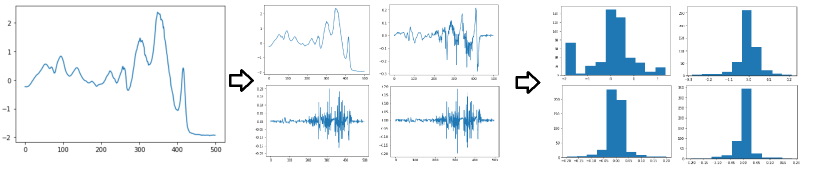
Figure 2: Illustration of the GeoDist pipeline. From a given time series, simple derivative-based quantities are extracted, and statistics of their distribution of values are given.

3.2 Defining and Extracting GeoStat Representation

The previous subsection detailed a number of quantities that are mathematically well-understood, are provably useful in determining a (smooth) time series, and are furthermore easy to compute in practice via standard finite difference approximations of derivatives. We wish to use all of these in a formulating the GeoStat (Geometric Statistics). Note that all of the quantities mentioned are functions of time. We proceed by ignoring that they are functions of time and merely consider the empirical distribution of each quantity mentioned. From the distributions of each quantity, we extract a sufficient number of statistics from each distribution such that if two sets of said statistics from two different time series are the same, then the distribution of their quantities are approximately equal.

To be more precise, for a given time series ${\bf{x}},$ we follow the below pipeline for extracting GeoStat representations. The basic idea is illustrated in Figure 2.

1. Upsample ${\bf{x}}$ if necessary using linear interpolation to reach the desired resolution of points

2. Apply the desired number of iterations of Laplacian smoothing in Equation (2), compute ${\bf{\dot{x}}}$, and apply the same number of iterations of Laplacian smoothing to ${\bf{\dot{x}}}.$

3. Compute ${\bf{\ddot{x}}},||{\bf{\ddot{x}}}||,$ and $||\kappa({\bf{x}})||,$ and smooth.

4. Extract empirical distributions of relevant features:

   • For univariate time series: ${\bf{x}},{\bf{\dot{x}}},{\bf{\ddot{x}}},$ the curvature, and the signed curvature.

   • For multivariate time series: ${\bf{x}},s_{\bf{x}},$ and $\dot{s}_{\bf{x}}$

   and other potentially relevant problem-dependent information, where each sample in the empirical distributions is the value of the corresponding feature at each time.

For real-valued distributions, we use the following statistics: range, mean, standard deviation, skew, kurtosis, and quantiles. This differs from those used in etemad2018predicting in a number of ways. Here, we extract skew and kurtosis in order to capture different notions of spread that are not well captured by the other features. In addition, we also use a more extensive set of quantiles, notably more quantiles towards the tails of each distribution so as to better capture extremal behavior.

For multivariate time series, position is not properly real-valued. Because of this, the resulting statistics that we can reasonably take are limited; quantiles, for example, do not make sense as there is no natural order to Euclidean space. We instead derive statistics based off of the following quantity:

$$\sigma^{2}(p)=\sum_{i=1}^{n}d^{2}(p_{i},p),$$ (5)

where the $p_{i}$ are points on the sphere and $d^{2}(\cdot,\cdot)$ is the squared distance between two points on the sphere. The minimum of this function is known as the Frechet variance, and any $p$ that attains this minimum is known as a Frechet mean. For Euclidean space, this is the usual mean; this quantity is, however, useful for spherical-valued and other non-Euclidean valued time series. Note that though the Frechet mean is in general not unique, it is if the $p_{i}$ in the summation are within a small enough neighborhood on the sphere karcher1977riemannian . In practice, it is easy to compute both quantities by brute force, and we did not run into any issues of nonuniqueness for the data considered. Note that the Frechet variance is always meaningful, even if the Frechet mean is not unique.

Features in GeoStat representations have some degree of sensitivity to various changes in a time series, in the sense that if a time series $\bf{x}$ is transformed into a time series $\bf{F(x)},$ then the features in time series $\bf{F(x)}$ differ from those in $\bf{x},$ albeit generally in a structured way. The resulting change of the quantities mentioned above to various transformations (e.g. offsets, scaling, drift, phase shifts, trend changes) can be analytically determined via derivative properties. Noise will ultimately result in fluctuations in all quantities depending on the structure of the smoothed noise. Per the pipeline, time series with missing values or discontinuities will have those resulting portions interpolated, incorporating these issues into the representation. Time series of unequal duration do not have this explicitly incorporated into their representation, though we encourage the reader to see both the next subsection as well as our discussion on the GFW vessel trajectory dataset GFWData ; GFWWebsite for ways to address this.

3.3 Representation by features on windows

GeoStat representations attempt to give a global summary of a given time series, with no explicit incorporation of notion of locality. This is perhaps a downside, as it has been observed in fawaz2019deep that modern deep learning classifiers may learn local features in order to make accurate predictions. Nevertheless, it is possible to easily adapt our proposed representation to incorporate local information via windowed GeoStat representaitons: compute all geometric quantities as above, divide the time series into windows, compute the statistical features on each window, and represent the entire time series as a concatenation of all of the features. This also allows for one to address potential unequal durations of time series: once can artificially continue shorter time series (by appending constant values), and then use a multi-window representation. One must take care in using such a representation, as the number of resulting features increases linearly in $k.$ Though how to choose both the number and location of windows used are immediate questions of interest, we do not explicitly pursue this and leave both questions for future work. That being said, we do show that windowed representations using the aforementioned features can result in substantial improvements in classification.

4 Evaluation and Comparison

4.1 Comparison on the Univariate UCR 2018 Archive

To illustrate the potential of GeoStat representations, we compare the results of KNN and SVM classifiers trained on these representation with recently proposed deep learning classifiers analyzed in fawaz2019deep ; fawaz2019git . Our benchmark of interest is the UCR 2018 Time Series Classification Repository dau2019ucr , a collection of 128 time series datasets from a variety of applications used to evaluate performance, with each dataset having its own fixed training and test sets. We follow fawaz2019deep ; fawaz2019git and measure the performance of each classifier by the mean accuracy averaged over five experiments. Note that fawaz2019deep ; fawaz2019git also reported the mean accuracy averaged over ten experiments for the UCR/UEA Repository, which is itself a subset of the UCR 2018 Repository; for completion, we report the mean accuracy over ten experiments on this smaller collection in the Appendix.

4.1.1 Experimental setup

We consider every dataset with the UCR 2018 Repository outside of Crop, for which we ran into memory issues during training. For the small number of datasets in which the individual time series were of unequal length, all time series were upsampled to have the same duration; those with smaller duration were appended with an appropriate number of zeros so as to ensure equal length. Each time series was linearly interpolated, if necessary, to have a minimum of 500 equally spaced samples in time. For each dataset, we construct twelve different feature representations based on the number of iterations of Laplacian smoothing (see Equation (2)) and number of windows employed (see the end of Section 3). We specifically consider 0, 1, and 2 iterations of Laplacian smoothing; we also use 1, 2, 4, and 6 windows created by dividing the whole time interval into the corresponding number of consecutive windows of equal length. These representations are then $z$-normalized, and used to train $k$-Nearest Neighbors (KNN) and Support Vector Machine (SVM) classifiers via 10-fold cross validation, with hyperparameters and other relevant quantities given in the Appendix.

Feature extraction was performed in Python3 using SciPy on a Windows 10 Laptop with a 2.2GHz i7-8750H CPU with 16 GB of RAM. Classification results for KNN and SVM models were obtained using Python3 and SciPy packages on an Ubuntu cluster with four 2.1 GHz Xeon Gold 6152 CPUs and 360 GB of RAM virtanen2020scipy . We limit our comparison to other single-model classifiers, namely those in fawaz2019deep ; fawaz2019git as well as the 1NN dynamic time warping benchmark. We specifically leave out both Time-CNN and t-LeNet due to their poor performance relative to other deep learning models tested, resulting in a total of seven deep learning methods.

4.1.2 Performance

Table 1: Ranking of 24 classifiers trained on our representation relative to seven deep learning models and 1-NN DTW on 127 datasets in the UCR 2018 Repository.

Model 1st 2nd 3rd 4th 5th 6th 7th 8th 9th KNN_1W_0S 10 3 22 11 13 12 18 16 22 KNN_1W_1S 12 3 21 15 11 10 15 19 21 KNN_1W_2S 10 3 24 14 14 9 16 14 23 KNN_2W_0S 11 7 25 18 15 13 12 15 11 KNN_2W_1S 14 7 20 19 21 13 13 10 10 KNN_2W_2S 12 7 25 20 21 9 18 9 6 KNN_4W_0S 19 7 26 21 11 11 10 15 7 KNN_4W_1S 16 13 23 21 16 9 13 10 6 KNN_4W_2S 20 10 23 20 12 18 12 8 4 KNN_6W_0S 13 14 24 23 17 10 11 9 6 KNN_6W_1S 17 10 24 22 17 14 14 5 4 KNN_6W_2S 19 10 22 31 11 13 9 7 5 SVM_1W_0S 16 6 27 17 17 11 7 11 15 SVM_1W_1S 15 10 30 17 11 12 10 10 12 SVM_1W_2S 18 11 26 17 11 12 11 13 8 SVM_2W_0S 15 12 27 29 16 6 10 9 3 SVM_2W_1S 22 12 31 24 9 7 12 9 1 SVM_2W_2S 20 14 35 18 13 11 7 6 3 SVM_4W_0S 21 15 33 20 14 12 5 5 2 SVM_4W_1S 23 17 31 27 8 8 7 4 2 SVM_4W_2S 28 15 32 24 7 9 7 4 1 SVM_6W_0S 23 10 28 23 16 14 8 4 1 SVM_6W_1S 27 13 28 25 14 8 8 3 1 SVM_6W_2S 27 13 36 20 12 10 6 3 0 Best KNN 37 12 28 25 8 7 5 3 2 Best SVM 48 19 34 16 3 4 3 0 0 Best Model 55 19 28 17 3 3 2 0 0

Because of the large number of datasets present in this repository, we defer most results to the Appendix and the Supplementary Material. In the main text, we present highlights that reinforce our claim that our representation can be used to create meaningful classifiers.

Table 1 summarizes our results by ranking their average performance over five iterations relative to seven of the deep learning models studied in fawaz2019deep and 1-NN DTW. All models trained under this representation are listed as XXX_YW_ZS, where XXX is the model in question, Y is the number of windows used, and Z is the number of Laplacian smoothing iterations used. We also consider, in a separate category, the ranking of the KNN and SVM models with maximum accuracy. For the sake of transparency and standardization, we obtained performance numbers for the deep learning models from fawaz2019git , and we obtained the numbers for 1-NN DTW from the UCR Time Series Repository website ucr2018website (note that the procedure used for DTW is deterministic). As ucr2018website lists three separate values for DTW (namely, no warping, a learned warping window, and a fixed warping window), we compare to the maximum of these for each dataset.

One immediately sees how well simple classifiers trained on our representation can perform. In particular, every SVM, as well as all KNN models trained on 4 and 6 window representations, performs better on average than over half of the other eight models considered on every dataset tested. This is perhaps surprising given both the relatively small training complexity of the models we train on our representation, as well as the wide variety of time series within the UCR 2018 Repository. Perhaps most astonishing is that for all but eight of the datasets considered, at least one of the models trained on our representation achieves better classification accuracy than over half of the other models considered. Of the eight datasets for which this is not true, four of the others (FordA, FordB, DodgerLoopGame, DodgerLoopWeekend) have significant high frequency components, which may indicate a weakness of restricting to only differential geometric components, though we do not investigate this further. It is not immediately as to what causes performance issues for the other datasets (Ham, ItalyPowerDemand, SyntheticControl, and TwoPatterns), though we note that at least one of these models is never the worst or second-worst performing per Table 1. This leaves little question: the particular representation we employ captures significant information necessary to characterize many types of time series.

Table 2: Ranking of the best models trained on our representation relative to each category in the UCR 2018 Repository.

Category 1st 2nd 3rd 4th 5th 6th 7th 8th 9th Power 1 0 0 0 0 0 0 0 0 HRM 1 0 0 0 0 0 0 0 0 Motion 7 5 1 3 0 0 1 0 0 Trajectory 1 0 2 0 0 0 0 0 0 Simulated 4 1 2 0 0 1 0 0 0 Traffic 0 1 1 0 0 0 0 0 0 Hemodynamics 1 1 1 0 0 0 0 0 0 Spectrum 3 0 1 0 0 0 0 0 0 EPG 2 0 0 0 0 0 0 0 0 Spectro 5 2 1 0 0 0 0 0 0 EOG 0 1 0 1 0 0 0 0 0 ECG 2 1 2 0 1 0 0 0 0 Sensor 8 2 10 7 2 1 0 0 0 Device 5 1 1 0 0 1 0 0 0 Image 15 4 6 6 0 0 1 0 0

It is natural to ask if the rankings in Table 1 are biased towards a particular type of data. We list this information in Table 2, where the categories are those listed in the UCR 2018 Repository. The only category for which the best GeoStat model is neither first nor second for the majority of the datasets is Sensor, giving credence to a potential weakness of our representation being significant high-frequency components. Other categories have one of the models trained on GeoStat representations within the top 2 of those considered.

We conclude this section with two remarks. First, we note per the Appendix that GeoStat representations allows for perfect classification for the given train/test splits on a number of datasets (e.g. Beef, BeetleFly, and BirdChicken) that have proven difficult for the other methods in our comparison. Second, given that we are proposing GeoStat representation in part as a reasonable DTW-free benchmark, we note that at least one of the models trained on our representation has average accuracy equal or better than that of the DTW accuracy we list on 106 of the 127 datasets considered. Though not perfect, given the relative simplicity of our methods, this does suggest that GeoStat representations can be used as such a benchmark provided sufficient hyperparameter tuning.

4.2 Multivariate Case Study: Vessel Classification

Table 3: Statistics of 10-fold nested cross validation scores for KNN and SVM with respect to the given features.

Model Min Max Mean Std KNN 0.6549 0.6883 0.6701 0.0079 SVM 0.6810 0.7028 0.6921 0.0061

As previously mentioned in Section 1, we will evaluate the performance of our method in the multivariate setting on a challenging dataset from Global Fishing Watch GFWData ; GFWWebsite . This dataset consists of 1258 vessel trajectories spanning the entire globe (a sphere) over a period of four years. Figure 1 shows the spatial range of one hundred of these trajectories (with some GPS errors) over this time period. Of these, 1107 are labeled with one of twelve different vessel classes. The goal is accurate classification. The current state of the art on this problem given in kroodsma2018tracking is a large CNN that was trained and tested on a much larger superset of the data freely available; we have approximately 2% of what was used. Their model achieves a high classification accuracy of approximately 95% on a fixed training set of 52,964 and a test set of 22,172. We are interested in seeing if the features employed combined with SVM and KNN models can yield good performance despite a lack of data. Note that this dataset requires a fair amount of preprocessing before we use it; details are given in the Appendix. In particular, irregular sampling rates are relevant to vessel behavior kroodsma2018tracking .

Given the geographic scope of the data, the dataset that we have to work with is itself relatively small. We ideally need access to as much data as possible, but formally holding out a fixed dataset would perhaps highly bias our result. We instead use 10-fold nested cross-validation, which allows us to generate random train-validation-test splits. To be more precise, we will first split the dataset into 10 parts of equal size. One of these parts will act as a holdout set. The other nine parts will be combined and then split into another 10 pieces, which we will run cross-validation on to tune hyperparameters (the same as in the previous section). Based on these chosen hyperparameters, the final loss is evaluated on the holdout set from the first split. This is repeated so that each of the folds is used as a holdout set; the final loss is the average of the losses for each holdout set.

We performed thirty iterations of this 10-fold nested cross validation procedure. Statistics of these iterations are given in Table 3. Both models perform surprisingly well in this scenario, with KNN and SVM achieving 67% and 69% accuracy on average, respectively, whereas approximately 50-times as much data with a deep learning model achieves 95% accuracy for a fixed train/test split. We give a confusion matrix in the Appendix for a fixed nested cross-validation iteration. In particular, note that a large amount of inaccuracy comes from confusing certain classes of vessels, such as reefers and cargo/tankers, which have similar movement patterns and are potentially mistakable by just trajectory information alone.

5 Empirical Studies

We discuss particular choices made in the course of constructing the presented GeoStat representations. Though some discussions will be based off of material presented in the main text, full details of many will be deferred to the Appendix.

5.1 Amount of Laplacian smoothings

Based on Table 1, we see a general pattern of improved performance with additional iterations of smoothing. This is not true of every model: KNN_1W_1S generally performs better than KNN_1W_2S. The general pattern, however, is perhaps not surprising; the Laplacian smoothing we employed effectively acts as a denoising algorithm.

5.2 Amount of Windows Used

A perhaps notable trend is the role of using more windows. By representing a time series by multiple windows, performance can significantly increase. This is most evident by comparing the 1-window SVM models to the 6-window SVM models. We again remark that our choice of windows was not algorithmic, and leave the possibility that one can learn a good choice of windows as future work.

5.3 Effect of specific windows

As discussed in fawaz2019deep , the success of deep learning on time series classification might be attributed to the ability to learn localized features; the performance of KNN and SVM with multiple windows suggests the same. To test this, we trained both KNN and SVM classifiers on the statistics from each of the individual windows extracted on the 6-window dataset with one smoothing iteration. Though restricting to individual windows does not appear to improve performance, near-perfect or perfect classification results can be achieved using only information from specific windows (e.g. Beef, BeetleFly, BirdChicken, and StarlightCurves). This suggests that future improvements on classification may rely on the ability for models to find local areas of interest, at least in certain cases. Other results show (e.g. on the Adiac and Cricket), however, that this is not true in general.

5.4 Parameter ablation studies

We conducted parameter ablation studies on each of the datasets studied. Specifically, we tested the effect of removing specific geometric features (e.g. position, curvature) and specific statistics on classifier performance. All tables are given in the Appendix, with the datasets from the UCR 2018 Repository separated into the categories given in Table 2 for brevity. Given both the breadth and the unequal amount of datasets per category, it is difficult to jump to conclusions; both the HRM and Power categories, for example, only have one dataset. The importance of both the position and velocity information is clear throughout, resulting in significant accuracy decreases when omitted. Similarly, extremal quantiles also appear to be beneficial for classifying time series in general. Perhaps the most contentious quantities involve second derivative information, being detrimental for some categories and important for others, noting again that some categories have very few datasets. Given this, we can only conclude the importance of position, velocity, and extremal quantile information in general, suggesting that the importance of other parameters be evaluated on a case by case basis.

6 Conclusion

We proposed GeoStat representations for time series, summarizing time series by summary statistics of distributions of geometric values. We showed that simple classifiers trained on these representations can be extremely competitive with modern single-model classifiers based on deep learning, as well as the gold standard 1NN-DTW benchmark, achieving state of the art performance on a number of real datasets. We also showed that such methods achieve good performance on the difficult, limited multivariate GFW dataset relative to that of the state of the art despite the small amount of data.

There are many directions for future work. As noted in Section 4, our representation may not be sufficient for characterizing time series with significant high frequency components. It is not clear if purely geometric quantities can address this, but doing so, preferably with well-understood mathematical quantities, is an immediate direction for future work. The particular choice of representing statistics lends itself to interesting questions. It is interesting to ask whether a more compact, or more mathematically natural representation of said distributions would have similar or better performance. Finally, as we discussed earlier, we did little work in investigating window choices. Though some of our results on restriction to particular windows were enlightening, further studies should be done to determine particular regions of interest for classification.

7 Appendix

7.1 Supplementary Material structure

The Supplementary Material is divided into two folders, one for the univariate experiments and one for the multivariate experiments. The results folder contains all data used for every result presented in the main paper and the Appendix, along with additional information for each set of experiments performed. Every model and window combination contains, for each dataset, the average accuracy over all runs of the same experiment, as well as the minimum/maximum accuracies and the standard deviation. These do not include the results from [17] or [24], which themselves are available on [16] and [24] respectively. We do, however, include the script that was used to extract the results from the raw results posted on [16]; the results from [24] were downloaded from the website and manually processed.

We include the processed data from the multivariate experiment, but due to size constraints, do not include any of the raw data nor any of the processed UCR data. The raw data can be obtained from [42] and [24], and we include all extraction scripts (with listed order for running) used in obtaining them. Those interested in doing so should only need to specify paths. However, it is important to note that both raw datasets (and the processed UCR dataset) are quite large. This may render personal verification infeasible without sufficient resources, though please note that none of the results were derived with GPUs.

7.2 Hyperparameters

The following hyperparameters were used for both univariate and multivariate tests. All variable names follow the same convention as in [39]

• KNN

  • n_neighbors: 1, 2, 4, 6, 8, 10

  • weights: ’uniform’,’distance’

  • p: 1,2

• SVM

  • C: 0.1, 1, 10

  • kernel: ’linear’,’rbf’,’poly’

  • degree: 2

7.3 Univariate comparison results

7.3.1 Quantiles

We employ the following quantiles: 0.001, 0.01, 0.1, 0.2, 0.3, 0.4, 0.5, 0.6, 0.7, 0.8, 0.9, 0.99, 0.999.

7.3.2 UCR 2018 Results

Table 4: Tables showing accuracy statistics for the UCR 2018 repository with five iterations of cross validation. The results listed here are for SVM (left) and KNN (right) trained on 4-window GeoStat representations with two iterations of Laplacian smoothing.

Dataset (SVM)	Min	Max	Mean	Std. Dev
ACSF1	0.6200	0.6500	0.6260	0.0120
Adiac	0.7775	0.7826	0.7785	0.0020
AllGestureWiimoteX	0.5471	0.5471	0.5471	0.0000
AllGestureWiimoteY	0.5900	0.5900	0.5900	0.0000
AllGestureWiimoteZ	0.5500	0.5500	0.5500	0.0000
ArrowHead	0.7371	0.7371	0.7371	0.0000
BME	0.9867	0.9867	0.9867	0.0000
Beef	0.7667	0.7667	0.7667	0.0000
BeetleFly	0.5000	0.9000	0.7100	0.1319
BirdChicken	0.9000	0.9000	0.9000	0.0000
CBF	0.9756	0.9756	0.9756	0.0000
Car	0.8333	0.8833	0.8533	0.0245
Chinatown	0.7522	0.7522	0.7522	0.0000
ChlorineConcentration	0.6901	0.6901	0.6901	0.0000
CinCECGTorso	0.9246	0.9246	0.9246	0.0000
Coffee	1.0000	1.0000	1.0000	0.0000
Computers	0.6000	0.6040	0.6032	0.0016
CricketX	0.6487	0.6487	0.6487	0.0000
CricketY	0.7000	0.7000	0.7000	0.0000
CricketZ	0.6359	0.6846	0.6749	0.0195
DiatomSizeReduction	0.9608	0.9608	0.9608	0.0000
DistalPhalanxOutlineAgeGroup	0.7338	0.7338	0.7338	0.0000
DistalPhalanxOutlineCorrect	0.7681	0.7717	0.7703	0.0018
DistalPhalanxTW	0.6691	0.6691	0.6691	0.0000
DodgerLoopDay	0.3500	0.4125	0.3625	0.0250
DodgerLoopGame	0.7391	0.7536	0.7507	0.0058
DodgerLoopWeekend	0.9710	0.9710	0.9710	0.0000
ECG200	0.8100	0.8400	0.8160	0.0120
ECG5000	0.9353	0.9362	0.9357	0.0004
ECGFiveDays	0.9501	0.9501	0.9501	0.0000
EOGHorizontalSignal	0.4890	0.5028	0.4917	0.0055
EOGVerticalSignal	0.4420	0.4448	0.4425	0.0011
Earthquakes	0.7338	0.7482	0.7424	0.0070
ElectricDevices	0.7041	0.7041	0.7041	0.0000
EthanolLevel	0.7580	0.7660	0.7644	0.0032
FaceAll	0.8018	0.8018	0.8018	0.0000
FaceFour	0.7841	0.7841	0.7841	0.0000
FacesUCR	0.8610	0.8610	0.8610	0.0000
FiftyWords	0.7604	0.7670	0.7618	0.0026
Fish	0.9257	0.9257	0.9257	0.0000
FordA	0.8242	0.8242	0.8242	0.0000
FordB	0.6617	0.6852	0.6711	0.0115
FreezerRegularTrain	0.9947	0.9947	0.9947	0.0000
FreezerSmallTrain	0.9744	0.9744	0.9744	0.0000
Fungi	0.8602	0.8602	0.8602	0.0000
GestureMidAirD1	0.6615	0.6615	0.6615	0.0000
GestureMidAirD2	0.4923	0.5538	0.5046	0.0246
GestureMidAirD3	0.3231	0.3231	0.3231	0.0000
GesturePebbleZ1	0.8430	0.8837	0.8756	0.0163
GesturePebbleZ2	0.7975	0.7975	0.7975	0.0000
GunPoint	1.0000	1.0000	1.0000	0.0000
GunPointAgeSpan	0.9842	0.9842	0.9842	0.0000
GunPointMaleVersusFemale	0.9842	0.9937	0.9892	0.0038
GunPointOldVersusYoung	1.0000	1.0000	1.0000	0.0000
Ham	0.6571	0.6762	0.6648	0.0093
HandOutlines	0.9324	0.9324	0.9324	0.0000
Haptics	0.4968	0.5195	0.5149	0.0091
Herring	0.6250	0.6406	0.6313	0.0077
HouseTwenty	0.9412	0.9664	0.9563	0.0124
InlineSkate	0.4891	0.5291	0.5211	0.0160
InsectEPGRegularTrain	1.0000	1.0000	1.0000	0.0000
InsectEPGSmallTrain	0.9719	0.9719	0.9719	0.0000
InsectWingbeatSound	0.5354	0.5753	0.5515	0.0194
ItalyPowerDemand	0.9378	0.9466	0.9396	0.0035
LargeKitchenAppliances	0.7200	0.7200	0.7200	0.0000
Lightning2	0.7377	0.7705	0.7443	0.0131
Lightning7	0.6438	0.6712	0.6603	0.0134
Mallat	0.9390	0.9390	0.9390	0.0000
Meat	0.9500	0.9500	0.9500	0.0000
MedicalImages	0.7092	0.7382	0.7324	0.0116
MelbournePedestrian	0.8963	0.9008	0.8991	0.0021
MiddlePhalanxOutlineAgeGroup	0.5260	0.6234	0.6039	0.0390
MiddlePhalanxOutlineCorrect	0.8351	0.8385	0.8371	0.0017
MiddlePhalanxTW	0.5974	0.5974	0.5974	0.0000
MixedShapesRegularTrain	0.9559	0.9654	0.9578	0.0038
MixedShapesSmallTrain	0.9320	0.9320	0.9320	0.0000
MoteStrain	0.8546	0.8546	0.8546	0.0000
NonInvasiveFetalECGThorax1	0.9226	0.9252	0.9232	0.0010
NonInvasiveFetalECGThorax2	0.9257	0.9262	0.9259	0.0002
OSULeaf	0.8182	0.8182	0.8182	0.0000
OliveOil	0.9000	0.9000	0.9000	0.0000
PLAID	0.6946	0.7002	0.6968	0.0018
PhalangesOutlinesCorrect	0.8077	0.8077	0.8077	0.0000
Phoneme	0.2959	0.2959	0.2959	0.0000
PickupGestureWiimoteZ	0.6600	0.6600	0.6600	0.0000
PigAirwayPressure	0.1587	0.1587	0.1587	0.0000
PigArtPressure	0.8462	0.8462	0.8462	0.0000
PigCVP	0.4423	0.4423	0.4423	0.0000
Plane	1.0000	1.0000	1.0000	0.0000
PowerCons	0.9389	0.9389	0.9389	0.0000
ProximalPhalanxOutlineAgeGroup	0.8585	0.8585	0.8585	0.0000
ProximalPhalanxOutlineCorrect	0.8454	0.8625	0.8488	0.0069
ProximalPhalanxTW	0.7707	0.8146	0.7971	0.0215
RefrigerationDevices	0.5653	0.5653	0.5653	0.0000
Rock	0.8000	0.8000	0.8000	0.0000
ScreenType	0.4507	0.4507	0.4507	0.0000
SemgHandGenderCh2	0.8833	0.9000	0.8867	0.0067
SemgHandMovementCh2	0.7178	0.7178	0.7178	0.0000
SemgHandSubjectCh2	0.8533	0.8533	0.8533	0.0000
ShakeGestureWiimoteZ	0.8800	0.8800	0.8800	0.0000
ShapeletSim	0.6278	0.6500	0.6411	0.0109
ShapesAll	0.8350	0.8350	0.8350	0.0000
SmallKitchenAppliances	0.7920	0.7920	0.7920	0.0000
SmoothSubspace	0.9533	0.9600	0.9560	0.0033
SonyAIBORobotSurface1	0.8419	0.8419	0.8419	0.0000
SonyAIBORobotSurface2	0.8940	0.8940	0.8940	0.0000
StarLightCurves	0.9772	0.9772	0.9772	0.0000
Strawberry	0.9541	0.9649	0.9627	0.0043
SwedishLeaf	0.9584	0.9584	0.9584	0.0000
Symbols	0.9618	0.9618	0.9618	0.0000
SyntheticControl	0.9600	0.9600	0.9600	0.0000
ToeSegmentation1	0.8509	0.8509	0.8509	0.0000
ToeSegmentation2	0.7462	0.7769	0.7523	0.0123
Trace	0.9900	0.9900	0.9900	0.0000
TwoLeadECG	0.9860	0.9860	0.9860	0.0000
TwoPatterns	0.9708	0.9708	0.9708	0.0000
UMD	0.9931	0.9931	0.9931	0.0000
UWaveGestureLibraryAll	0.9453	0.9497	0.9489	0.0018
UWaveGestureLibraryX	0.8082	0.8082	0.8082	0.0000
UWaveGestureLibraryY	0.7457	0.7457	0.7457	0.0000
UWaveGestureLibraryZ	0.7440	0.7440	0.7440	0.0000
Wafer	0.9927	0.9927	0.9927	0.0000
Wine	0.5741	0.8704	0.6926	0.1452
WordSynonyms	0.6411	0.6897	0.6605	0.0238
Worms	0.7143	0.7143	0.7143	0.0000
WormsTwoClass	0.7532	0.8052	0.7948	0.0208
Yoga	0.8623	0.8623	0.8623	0.0000

Dataset (KNN)	Min	Max	Mean	Std. Dev
ACSF1	0.7600	0.7600	0.7600	0.0000
Adiac	0.7084	0.7084	0.7084	0.0000
AllGestureWiimoteX	0.5800	0.5800	0.5800	0.0000
AllGestureWiimoteY	0.5414	0.6171	0.6020	0.0303
AllGestureWiimoteZ	0.5971	0.5971	0.5971	0.0000
ArrowHead	0.7886	0.7886	0.7886	0.0000
BME	0.9600	0.9600	0.9600	0.0000
Beef	0.5667	0.5667	0.5667	0.0000
BeetleFly	0.7000	0.8000	0.7400	0.0490
BirdChicken	0.8000	0.8000	0.8000	0.0000
CBF	0.9656	0.9711	0.9667	0.0022
Car	0.7167	0.7833	0.7533	0.0245
Chinatown	0.9242	0.9679	0.9592	0.0175
ChlorineConcentration	0.6693	0.6693	0.6693	0.0000
CinCECGTorso	0.8406	0.8406	0.8406	0.0000
Coffee	0.9643	1.0000	0.9714	0.0143
Computers	0.6080	0.6480	0.6272	0.0139
CricketX	0.6231	0.6231	0.6231	0.0000
CricketY	0.6359	0.6359	0.6359	0.0000
CricketZ	0.6282	0.6436	0.6333	0.0056
DiatomSizeReduction	0.9379	0.9379	0.9379	0.0000
DistalPhalanxOutlineAgeGroup	0.7122	0.7194	0.7137	0.0029
DistalPhalanxOutlineCorrect	0.7500	0.7500	0.7500	0.0000
DistalPhalanxTW	0.6331	0.6475	0.6446	0.0058
DodgerLoopDay	0.3625	0.4500	0.4100	0.0278
DodgerLoopGame	0.7464	0.7464	0.7464	0.0000
DodgerLoopWeekend	0.9493	0.9710	0.9609	0.0098
ECG200	0.8000	0.8000	0.8000	0.0000
ECG5000	0.9413	0.9433	0.9421	0.0010
ECGFiveDays	0.8955	0.8955	0.8955	0.0000
EOGHorizontalSignal	0.3619	0.4061	0.3796	0.0165
EOGVerticalSignal	0.3177	0.3591	0.3508	0.0166
Earthquakes	0.7338	0.7482	0.7424	0.0070
ElectricDevices	0.6631	0.6681	0.6659	0.0023
EthanolLevel	0.4240	0.4240	0.4240	0.0000
FaceAll	0.7550	0.8515	0.7936	0.0473
FaceFour	0.7727	0.8409	0.7864	0.0273
FacesUCR	0.8059	0.8420	0.8343	0.0143
FiftyWords	0.7187	0.7187	0.7187	0.0000
Fish	0.8514	0.8743	0.8663	0.0078
FordA	0.7174	0.7197	0.7183	0.0011
FordB	0.6827	0.6889	0.6872	0.0024
FreezerRegularTrain	0.9544	0.9740	0.9667	0.0068
FreezerSmallTrain	0.9288	0.9309	0.9292	0.0008
Fungi	0.9409	0.9409	0.9409	0.0000
GestureMidAirD1	0.5923	0.6231	0.6046	0.0151
GestureMidAirD2	0.5077	0.5077	0.5077	0.0000
GestureMidAirD3	0.2385	0.2769	0.2523	0.0141
GesturePebbleZ1	0.8430	0.8547	0.8512	0.0047
GesturePebbleZ2	0.6519	0.7658	0.7114	0.0362
GunPoint	0.9933	0.9933	0.9933	0.0000
GunPointAgeSpan	1.0000	1.0000	1.0000	0.0000
GunPointMaleVersusFemale	0.9968	0.9968	0.9968	0.0000
GunPointOldVersusYoung	1.0000	1.0000	1.0000	0.0000
Ham	0.5905	0.6000	0.5981	0.0038
HandOutlines	0.8892	0.8919	0.8897	0.0011
Haptics	0.4513	0.4740	0.4669	0.0083
Herring	0.5938	0.7500	0.6750	0.0636
HouseTwenty	0.9412	0.9412	0.9412	0.0000
InlineSkate	0.5782	0.5782	0.5782	0.0000
InsectEPGRegularTrain	0.9920	0.9920	0.9920	0.0000
InsectEPGSmallTrain	0.9880	0.9880	0.9880	0.0000
InsectWingbeatSound	0.4808	0.5005	0.4927	0.0068
ItalyPowerDemand	0.9388	0.9388	0.9388	0.0000
LargeKitchenAppliances	0.6640	0.6960	0.6768	0.0157
Lightning2	0.7377	0.8197	0.8033	0.0328
Lightning7	0.6712	0.6712	0.6712	0.0000
Mallat	0.9684	0.9684	0.9684	0.0000
Meat	0.9000	0.9500	0.9367	0.0194
MedicalImages	0.6526	0.6974	0.6845	0.0161
MelbournePedestrian	0.9147	0.9184	0.9162	0.0018
MiddlePhalanxOutlineAgeGroup	0.5455	0.5909	0.5610	0.0195
MiddlePhalanxOutlineCorrect	0.7904	0.7904	0.7904	0.0000
MiddlePhalanxTW	0.5390	0.5779	0.5584	0.0123
MixedShapesRegularTrain	0.9588	0.9588	0.9588	0.0000
MixedShapesSmallTrain	0.9229	0.9328	0.9308	0.0040
MoteStrain	0.8578	0.8578	0.8578	0.0000
NonInvasiveFetalECGThorax1	0.8656	0.8687	0.8663	0.0012
NonInvasiveFetalECGThorax2	0.8707	0.8728	0.8711	0.0008
OSULeaf	0.6983	0.8140	0.7744	0.0430
OliveOil	0.8333	0.9333	0.8867	0.0452
PLAID	0.7486	0.7747	0.7695	0.0104
PhalangesOutlinesCorrect	0.7821	0.7890	0.7862	0.0034
Phoneme	0.2126	0.2748	0.2563	0.0224
PickupGestureWiimoteZ	0.5400	0.6800	0.5840	0.0571
PigAirwayPressure	0.0962	0.1731	0.1577	0.0308
PigArtPressure	0.9038	0.9038	0.9038	0.0000
PigCVP	0.4471	0.4471	0.4471	0.0000
Plane	1.0000	1.0000	1.0000	0.0000
PowerCons	0.8611	0.9056	0.8933	0.0163
ProximalPhalanxOutlineAgeGroup	0.8390	0.8585	0.8507	0.0073
ProximalPhalanxOutlineCorrect	0.8179	0.8213	0.8192	0.0017
ProximalPhalanxTW	0.7902	0.8098	0.8010	0.0089
RefrigerationDevices	0.4747	0.5173	0.4917	0.0209
Rock	0.6600	0.6600	0.6600	0.0000
ScreenType	0.4187	0.4533	0.4384	0.0161
SemgHandGenderCh2	0.9267	0.9483	0.9353	0.0106
SemgHandMovementCh2	0.7978	0.8000	0.7996	0.0009
SemgHandSubjectCh2	0.8444	0.8600	0.8520	0.0064
ShakeGestureWiimoteZ	0.7400	0.7400	0.7400	0.0000
ShapeletSim	0.5833	0.6611	0.6322	0.0286
ShapesAll	0.8433	0.8433	0.8433	0.0000
SmallKitchenAppliances	0.7467	0.7467	0.7467	0.0000
SmoothSubspace	0.9467	0.9800	0.9547	0.0129
SonyAIBORobotSurface1	0.8602	0.8602	0.8602	0.0000
SonyAIBORobotSurface2	0.7754	0.8006	0.7943	0.0098
StarLightCurves	0.9720	0.9751	0.9735	0.0013
Strawberry	0.9486	0.9541	0.9519	0.0026
SwedishLeaf	0.9312	0.9312	0.9312	0.0000
Symbols	0.9397	0.9397	0.9397	0.0000
SyntheticControl	0.9233	0.9233	0.9233	0.0000
ToeSegmentation1	0.6228	0.7325	0.7044	0.0425
ToeSegmentation2	0.7538	0.7846	0.7785	0.0123
Trace	1.0000	1.0000	1.0000	0.0000
TwoLeadECG	0.8060	0.9298	0.8325	0.0488
TwoPatterns	0.7553	0.7718	0.7675	0.0062
UMD	0.8958	0.9792	0.9556	0.0327
UWaveGestureLibraryAll	0.9196	0.9327	0.9222	0.0052
UWaveGestureLibraryX	0.7889	0.8102	0.8012	0.0100
UWaveGestureLibraryY	0.7384	0.7471	0.7453	0.0035
UWaveGestureLibraryZ	0.7401	0.7420	0.7417	0.0008
Wafer	0.9927	0.9935	0.9933	0.0003
Wine	0.6296	0.6296	0.6296	0.0000
WordSynonyms	0.6708	0.7053	0.6984	0.0138
Worms	0.7143	0.7403	0.7299	0.0127
WormsTwoClass	0.7403	0.7403	0.7403	0.0000
Yoga	0.8480	0.8480	0.8480	0.0000

We list full results for the UCR 2018 repository (minus Crop, as previously mentioned) for both KNN and SVM models trained on 4-window GeoStat representations with two iterations of Laplacian smoothing. Table 4. All results were taken over five iterations of cross validation. Of particular interest is the generally small standard deviation over the multiple iterations of cross validation. This is in stark contrast to the much larger variation found in the results of deep learning models in [17].

Table 5: Tables showing accuracy statistics for the UCR 2018 repository with 10 iterations of cross validation. The results listed here are for SVM (left) and KNN (right) trained on 4-window GeoStat representations with two iterations of Laplacian smoothing.

Dataset (SVM)	Min	Max	Mean	Std. Dev
ACSF1	0.6200	0.6500	0.6230	0.0090
Adiac	0.7775	0.7826	0.7780	0.0015
AllGestureWiimoteX	0.5471	0.5471	0.5471	0.0000
AllGestureWiimoteY	0.5557	0.5900	0.5866	0.0103
AllGestureWiimoteZ	0.5500	0.5500	0.5500	0.0000
ArrowHead	0.7371	0.7371	0.7371	0.0000
BME	0.9867	0.9867	0.9867	0.0000
Beef	0.7667	0.7667	0.7667	0.0000
BeetleFly	0.5000	0.9000	0.6750	0.1146
BirdChicken	0.9000	0.9000	0.9000	0.0000
CBF	0.9544	0.9756	0.9734	0.0063
Car	0.8333	0.8833	0.8667	0.0211
Chinatown	0.7522	0.7522	0.7522	0.0000
ChlorineConcentration	0.6901	0.6901	0.6901	0.0000
CinCECGTorso	0.9246	0.9246	0.9246	0.0000
Coffee	1.0000	1.0000	1.0000	0.0000
Computers	0.5800	0.6040	0.6012	0.0072
CricketX	0.6487	0.6487	0.6487	0.0000
CricketY	0.7000	0.7000	0.7000	0.0000
CricketZ	0.6359	0.6846	0.6797	0.0146
DiatomSizeReduction	0.9608	0.9608	0.9608	0.0000
DistalPhalanxOutlineAgeGroup	0.7338	0.7338	0.7338	0.0000
DistalPhalanxOutlineCorrect	0.7681	0.7717	0.7710	0.0014
DistalPhalanxTW	0.6691	0.6691	0.6691	0.0000
DodgerLoopDay	0.3500	0.4125	0.3625	0.0250
DodgerLoopGame	0.7391	0.7536	0.7522	0.0043
DodgerLoopWeekend	0.9493	0.9710	0.9688	0.0065
ECG200	0.8100	0.8400	0.8210	0.0137
ECG5000	0.9224	0.9362	0.9342	0.0039
ECGFiveDays	0.9501	0.9501	0.9501	0.0000
EOGHorizontalSignal	0.4890	0.5028	0.4931	0.0063
EOGVerticalSignal	0.4420	0.4448	0.4431	0.0014
Earthquakes	0.7338	0.7482	0.7410	0.0072
ElectricDevices	0.7041	0.7041	0.7041	0.0000
EthanolLevel	0.7580	0.7660	0.7652	0.0024
FaceAll	0.8018	0.8018	0.8018	0.0000
FaceFour	0.7841	0.8977	0.7955	0.0341
FacesUCR	0.8561	0.8610	0.8595	0.0022
FiftyWords	0.7604	0.7670	0.7624	0.0030
Fish	0.9257	0.9257	0.9257	0.0000
FordA	0.8242	0.8242	0.8242	0.0000
FordB	0.6617	0.6852	0.6758	0.0115
FreezerRegularTrain	0.9947	0.9947	0.9947	0.0000
FreezerSmallTrain	0.9744	0.9744	0.9744	0.0000
Fungi	0.8602	0.8602	0.8602	0.0000
GestureMidAirD1	0.6615	0.6615	0.6615	0.0000
GestureMidAirD2	0.4923	0.5538	0.5046	0.0246
GestureMidAirD3	0.2769	0.3231	0.3185	0.0138
GesturePebbleZ1	0.8430	0.8837	0.8634	0.0203
GesturePebbleZ2	0.7975	0.7975	0.7975	0.0000
GunPoint	1.0000	1.0000	1.0000	0.0000
GunPointAgeSpan	0.9842	0.9842	0.9842	0.0000
GunPointMaleVersusFemale	0.9842	0.9937	0.9889	0.0041
GunPointOldVersusYoung	1.0000	1.0000	1.0000	0.0000
Ham	0.6571	0.6762	0.6667	0.0095
HandOutlines	0.9324	0.9324	0.9324	0.0000
Haptics	0.4968	0.5195	0.5081	0.0114
Herring	0.6250	0.6406	0.6359	0.0072
HouseTwenty	0.9412	0.9664	0.9538	0.0126
InlineSkate	0.4891	0.5291	0.5211	0.0160
InsectEPGRegularTrain	1.0000	1.0000	1.0000	0.0000
InsectEPGSmallTrain	0.9719	0.9719	0.9719	0.0000
InsectWingbeatSound	0.5354	0.5753	0.5516	0.0193
ItalyPowerDemand	0.9378	0.9466	0.9396	0.0035
LargeKitchenAppliances	0.7200	0.7200	0.7200	0.0000
Lightning2	0.7377	0.7705	0.7410	0.0098
Lightning7	0.6438	0.6712	0.6521	0.0126
Mallat	0.9390	0.9390	0.9390	0.0000
Meat	0.9500	0.9500	0.9500	0.0000
MedicalImages	0.7092	0.7382	0.7353	0.0087
MelbournePedestrian	0.8963	0.9008	0.8990	0.0022
MiddlePhalanxOutlineAgeGroup	0.5260	0.6234	0.6039	0.0390
MiddlePhalanxOutlineCorrect	0.8351	0.8385	0.8378	0.0014
MiddlePhalanxTW	0.5974	0.5974	0.5974	0.0000
MixedShapesRegularTrain	0.9559	0.9654	0.9568	0.0028
MixedShapesSmallTrain	0.9320	0.9320	0.9320	0.0000
MoteStrain	0.8546	0.8546	0.8546	0.0000
NonInvasiveFetalECGThorax1	0.9226	0.9252	0.9232	0.0010
NonInvasiveFetalECGThorax2	0.9257	0.9262	0.9258	0.0002
OSULeaf	0.8182	0.8182	0.8182	0.0000
OliveOil	0.9000	0.9000	0.9000	0.0000
PLAID	0.6946	0.7095	0.6980	0.0041
PhalangesOutlinesCorrect	0.8077	0.8077	0.8077	0.0000
Phoneme	0.2959	0.2959	0.2959	0.0000
PickupGestureWiimoteZ	0.6600	0.6600	0.6600	0.0000
PigAirwayPressure	0.1587	0.1587	0.1587	0.0000
PigArtPressure	0.8462	0.8462	0.8462	0.0000
PigCVP	0.4423	0.4423	0.4423	0.0000
Plane	1.0000	1.0000	1.0000	0.0000
PowerCons	0.9389	0.9389	0.9389	0.0000
ProximalPhalanxOutlineAgeGroup	0.8585	0.8585	0.8585	0.0000
ProximalPhalanxOutlineCorrect	0.8454	0.8625	0.8488	0.0069
ProximalPhalanxTW	0.7707	0.8146	0.7795	0.0176
RefrigerationDevices	0.5013	0.5653	0.5589	0.0192
Rock	0.8000	0.8000	0.8000	0.0000
ScreenType	0.4507	0.4507	0.4507	0.0000
SemgHandGenderCh2	0.8833	0.9000	0.8883	0.0076
SemgHandMovementCh2	0.7178	0.7178	0.7178	0.0000
SemgHandSubjectCh2	0.8222	0.8533	0.8502	0.0093
ShakeGestureWiimoteZ	0.8800	0.8800	0.8800	0.0000
ShapeletSim	0.6278	0.6500	0.6367	0.0109
ShapesAll	0.8350	0.8350	0.8350	0.0000
SmallKitchenAppliances	0.7920	0.7920	0.7920	0.0000
SmoothSubspace	0.9533	0.9600	0.9573	0.0033
SonyAIBORobotSurface1	0.8419	0.8419	0.8419	0.0000
SonyAIBORobotSurface2	0.8940	0.8940	0.8940	0.0000
StarLightCurves	0.9772	0.9772	0.9772	0.0000
Strawberry	0.9541	0.9649	0.9638	0.0032
SwedishLeaf	0.9584	0.9584	0.9584	0.0000
Symbols	0.9618	0.9618	0.9618	0.0000
SyntheticControl	0.9600	0.9700	0.9610	0.0030
ToeSegmentation1	0.8509	0.8509	0.8509	0.0000
ToeSegmentation2	0.7154	0.7769	0.7523	0.0185
Trace	0.9900	0.9900	0.9900	0.0000
TwoLeadECG	0.9860	0.9860	0.9860	0.0000
TwoPatterns	0.9708	0.9708	0.9708	0.0000
UMD	0.9931	0.9931	0.9931	0.0000
UWaveGestureLibraryAll	0.9430	0.9497	0.9486	0.0023
UWaveGestureLibraryX	0.8082	0.8082	0.8082	0.0000
UWaveGestureLibraryY	0.7457	0.7457	0.7457	0.0000
UWaveGestureLibraryZ	0.7440	0.7440	0.7440	0.0000
Wafer	0.9927	0.9943	0.9929	0.0005
Wine	0.5741	0.8704	0.7222	0.1481
WordSynonyms	0.6411	0.6897	0.6654	0.0243
Worms	0.7143	0.7143	0.7143	0.0000
WormsTwoClass	0.8052	0.8052	0.8052	0.0000
Yoga	0.8623	0.8623	0.8623	0.0000

Dataset (KNN)	Min	Max	Mean	Std. Dev
ACSF1	0.7600	0.7600	0.7600	0.0000
Adiac	0.7084	0.7366	0.7113	0.0084
AllGestureWiimoteX	0.5800	0.5800	0.5800	0.0000
AllGestureWiimoteY	0.5414	0.6171	0.6096	0.0227
AllGestureWiimoteZ	0.5971	0.5971	0.5971	0.0000
ArrowHead	0.7886	0.7886	0.7886	0.0000
BME	0.9600	0.9600	0.9600	0.0000
Beef	0.5667	0.7333	0.5833	0.0500
BeetleFly	0.7000	0.8000	0.7200	0.0400
BirdChicken	0.8000	0.8000	0.8000	0.0000
CBF	0.9656	0.9800	0.9676	0.0045
Car	0.7167	0.7833	0.7583	0.0214
Chinatown	0.9242	0.9738	0.9641	0.0134
ChlorineConcentration	0.6693	0.6693	0.6693	0.0000
CinCECGTorso	0.8406	0.8406	0.8406	0.0000
Coffee	0.9643	1.0000	0.9679	0.0107
Computers	0.6080	0.6480	0.6288	0.0135
CricketX	0.6231	0.6333	0.6241	0.0031
CricketY	0.6359	0.6359	0.6359	0.0000
CricketZ	0.6282	0.6436	0.6323	0.0045
DiatomSizeReduction	0.9379	0.9379	0.9379	0.0000
DistalPhalanxOutlineAgeGroup	0.7050	0.7194	0.7108	0.0043
DistalPhalanxOutlineCorrect	0.7500	0.7500	0.7500	0.0000
DistalPhalanxTW	0.6115	0.6547	0.6432	0.0117
DodgerLoopDay	0.3625	0.4500	0.4063	0.0218
DodgerLoopGame	0.7464	0.7464	0.7464	0.0000
DodgerLoopWeekend	0.9493	0.9710	0.9659	0.0086
ECG200	0.8000	0.8400	0.8080	0.0160
ECG5000	0.9413	0.9433	0.9421	0.0010
ECGFiveDays	0.8955	0.8955	0.8955	0.0000
EOGHorizontalSignal	0.3453	0.4061	0.3696	0.0184
EOGVerticalSignal	0.3177	0.3785	0.3586	0.0154
Earthquakes	0.7338	0.7482	0.7410	0.0064
ElectricDevices	0.6631	0.6681	0.6650	0.0024
EthanolLevel	0.4080	0.4460	0.4246	0.0086
FaceAll	0.7550	0.8515	0.7840	0.0442
FaceFour	0.7727	0.8409	0.7864	0.0273
FacesUCR	0.8059	0.8420	0.8376	0.0106
FiftyWords	0.6989	0.7187	0.7167	0.0059
Fish	0.8457	0.8743	0.8634	0.0094
FordA	0.7174	0.7318	0.7212	0.0054
FordB	0.6827	0.6889	0.6875	0.0019
FreezerRegularTrain	0.9544	0.9740	0.9653	0.0074
FreezerSmallTrain	0.9288	0.9309	0.9290	0.0006
Fungi	0.9409	0.9409	0.9409	0.0000
GestureMidAirD1	0.5923	0.6231	0.6108	0.0151
GestureMidAirD2	0.5000	0.5077	0.5069	0.0023
GestureMidAirD3	0.2385	0.3385	0.2615	0.0284
GesturePebbleZ1	0.8430	0.8895	0.8564	0.0116
GesturePebbleZ2	0.6519	0.7658	0.7114	0.0257
GunPoint	0.9933	0.9933	0.9933	0.0000
GunPointAgeSpan	1.0000	1.0000	1.0000	0.0000
GunPointMaleVersusFemale	0.9968	0.9968	0.9968	0.0000
GunPointOldVersusYoung	1.0000	1.0000	1.0000	0.0000
Ham	0.5714	0.6000	0.5952	0.0088
HandOutlines	0.8892	0.8919	0.8900	0.0012
Haptics	0.4448	0.4740	0.4643	0.0111
Herring	0.5938	0.7500	0.6547	0.0543
HouseTwenty	0.9244	0.9412	0.9395	0.0050
InlineSkate	0.5782	0.5782	0.5782	0.0000
InsectEPGRegularTrain	0.9920	0.9920	0.9920	0.0000
InsectEPGSmallTrain	0.9880	0.9880	0.9880	0.0000
InsectWingbeatSound	0.4808	0.5081	0.4957	0.0078
ItalyPowerDemand	0.9388	0.9388	0.9388	0.0000
LargeKitchenAppliances	0.6640	0.6960	0.6832	0.0157
Lightning2	0.7377	0.8197	0.8115	0.0246
Lightning7	0.6712	0.6712	0.6712	0.0000
Mallat	0.9684	0.9684	0.9684	0.0000
Meat	0.9000	0.9500	0.9433	0.0153
MedicalImages	0.6526	0.7132	0.6950	0.0169
MelbournePedestrian	0.9147	0.9184	0.9155	0.0015
MiddlePhalanxOutlineAgeGroup	0.5455	0.5974	0.5630	0.0219
MiddlePhalanxOutlineCorrect	0.7904	0.7904	0.7904	0.0000
MiddlePhalanxTW	0.5390	0.5779	0.5591	0.0089
MixedShapesRegularTrain	0.9588	0.9588	0.9588	0.0000
MixedShapesSmallTrain	0.9134	0.9328	0.9299	0.0062
MoteStrain	0.8578	0.8858	0.8606	0.0084
NonInvasiveFetalECGThorax1	0.8656	0.8687	0.8660	0.0009
NonInvasiveFetalECGThorax2	0.8707	0.8728	0.8712	0.0008
OSULeaf	0.6983	0.8140	0.7777	0.0337
OliveOil	0.8333	0.9333	0.8733	0.0442
PLAID	0.7486	0.7747	0.7721	0.0078
PhalangesOutlinesCorrect	0.7821	0.7890	0.7876	0.0028
Phoneme	0.2126	0.2748	0.2532	0.0232
PickupGestureWiimoteZ	0.5400	0.7000	0.5780	0.0610
PigAirwayPressure	0.0962	0.1731	0.1577	0.0308
PigArtPressure	0.9038	0.9038	0.9038	0.0000
PigCVP	0.4471	0.4471	0.4471	0.0000
Plane	1.0000	1.0000	1.0000	0.0000
PowerCons	0.8611	0.9056	0.8972	0.0122
ProximalPhalanxOutlineAgeGroup	0.8390	0.8585	0.8517	0.0076
ProximalPhalanxOutlineCorrect	0.8179	0.8247	0.8199	0.0027
ProximalPhalanxTW	0.7902	0.8098	0.8044	0.0074
RefrigerationDevices	0.4747	0.5173	0.4875	0.0196
Rock	0.6600	0.7600	0.6900	0.0458
ScreenType	0.3760	0.4533	0.4368	0.0239
SemgHandGenderCh2	0.9267	0.9483	0.9332	0.0099
SemgHandMovementCh2	0.7978	0.8000	0.7993	0.0010
SemgHandSubjectCh2	0.8444	0.8600	0.8544	0.0068
ShakeGestureWiimoteZ	0.7400	0.7800	0.7440	0.0120
ShapeletSim	0.5833	0.6611	0.6244	0.0302
ShapesAll	0.8433	0.8433	0.8433	0.0000
SmallKitchenAppliances	0.7200	0.7467	0.7413	0.0107
SmoothSubspace	0.9467	0.9800	0.9540	0.0131
SonyAIBORobotSurface1	0.8602	0.8602	0.8602	0.0000
SonyAIBORobotSurface2	0.7754	0.8006	0.7962	0.0075
StarLightCurves	0.9720	0.9758	0.9738	0.0014
Strawberry	0.9486	0.9541	0.9503	0.0025
SwedishLeaf	0.9312	0.9312	0.9312	0.0000
Symbols	0.9397	0.9397	0.9397	0.0000
SyntheticControl	0.9233	0.9233	0.9233	0.0000
ToeSegmentation1	0.6228	0.7325	0.7154	0.0331
ToeSegmentation2	0.7538	0.8154	0.7831	0.0145
Trace	1.0000	1.0000	1.0000	0.0000
TwoLeadECG	0.7849	0.9298	0.8417	0.0577
TwoPatterns	0.7553	0.7718	0.7684	0.0045
UMD	0.8958	0.9792	0.9639	0.0265
UWaveGestureLibraryAll	0.9196	0.9327	0.9248	0.0064
UWaveGestureLibraryX	0.7889	0.8102	0.7971	0.0100
UWaveGestureLibraryY	0.7306	0.7471	0.7433	0.0060
UWaveGestureLibraryZ	0.7401	0.7420	0.7415	0.0009
Wafer	0.9927	0.9935	0.9934	0.0002
Wine	0.5926	0.6296	0.6259	0.0111
WordSynonyms	0.6708	0.7053	0.6984	0.0138
Worms	0.7143	0.7403	0.7351	0.0104
WormsTwoClass	0.7143	0.7403	0.7325	0.0119
Yoga	0.8480	0.8480	0.8480	0.0000

Table 5 displays the same results with 10 iterations of cross validation, as is done or the UCR/UEA subset in [17]. The results listed are consistent with those in Table 4.

NOTE FOR REVIEWERS: A sentence in the main text concerning perfect classification for some datasets was meant to be removed in the review draft but mistakenly was left in. As evidenced by Table 4 and the Supplementary Material, that statement is clearly not true and will be removed in the camera-ready version. We apologize for misleading anyone with its accidental conclusion. All data reported in the Appendix can be found in the Supplementary Material and is directly reproducible by the scripts given.

7.4 Vessel classification details

In the following we detail all processing done on the vessel classification dataset. This dataset has a number of challenges, such as large periods of inactivity, that must be dealt with before classifying

7.4.1 Incorporating sampling rate

Each vessel trajectory in [42] is sampled nonuniformly and asychronously of one another. The sampling rate for a given vessel is correlated with ocean traffic: if a vessel is around a large number of other vessels, then its sampling rate is more likely to decrease [25]. The number of neighbors of a given vessel (in some radius) was incorporated as a feature used in [25]. Given the lack of data that we have access to compared to [25], it is not reasonable to expect that such a feature will contain as much information in our case. Nevertheless, the sampling rate may act as a proxy that allows us to incorporate neighbor information. Thus, in addition for the geometric features considered, we also consider distributions based on the sampling rate. More specifically, we consider distributions of lengths of times in which each vessel falls into one of three classifications determined by its speed and sampling rate: active, inactive, and unknown.

Active time periods are those in which the vessel is moving at a speed greater than or equal to a predefined threshold, whereas inactive time periods are those where the vessel is moving at a speed less than said threshold. Note that it is natural for a vessel to be periodically inactive (e.g. not in use). We specifically chose 0.4 knots as the threshold. For active time periods, all previously mentioned geometric quantities are relevant. For inactive times, the only relevant quantity is the length of period of inactivity; vessels are otherwise almost stationary.

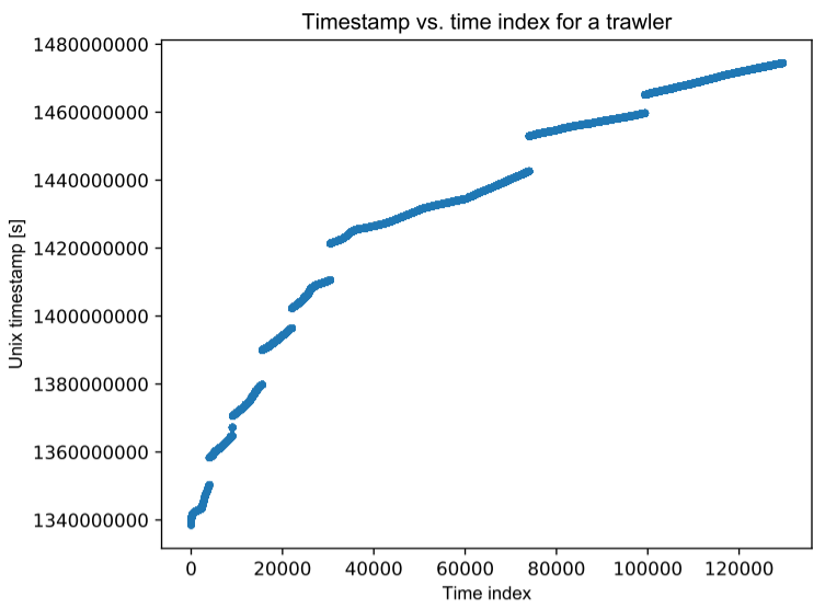
Figure 3: The time values (in Unix time) of the first timestamps for a trawler. Each unit is one second.

We define an unknown time period to be one in which the amount of time between consecutive samples of a trajectory is at least a minimum threshold; we chose 90 minutes. The length of time between any two samples of a vessel can be quite high; Figure 3 shows the potential length of gaps for one vessel. Distribution-wise, we consider the distribution of the lengths of time between samples provided that the time between samples is at least 90 minutes. This will act as a proxy for the amount of neighbors a vessel has at any point of time.

7.4.2 Additional features

We augment our GeoStat representation a number of other relevant features within our analysis. Two features of interest in this vessel classification problem, distance to shore and distance to port, are given for each trajectory at each time. We also use two variants of the curvature feature defined in the main text: the one proposed, and one obtained without any Laplacian smoothing after differentiating. Using both in tandem gives a multiscale notion of curvature, which initial experiments found important for establishing optimal performance.

7.4.3 Quantiles

We employ the following quantiles: 0.001, 0.01, 0.05, 0.1, 0.25, 0.5, 0.75, 0.9, 0.95, 0.99, 0.999.

7.4.4 Preprocessing

Not all of the 1258 trajectories available in [42] are immediately usable. A number of these trajectories, for example, do not have a well defined vessel label. Per the supplementary information in [25], this would suggest a classification of ”other fishing” or ”gear/buoy’ for each such vessel. Given that the former represents a catch-all category for fishing vessels (for which motion pattern is decidedly unclear) and those in the latter category are not actually vessels, we chose to ignore these in subsequent algorithm development. Note that the performance analysis in [25] did not explicitly consider the gear/buoy class, and achieved approximately 50% classification accuracy in test, so our decision is not without practical merit. We also chose to remove vessels that did not exhibit any periods of inactivity or any long sampling times; only seven vessels satisfied this property, creating minimal effect. This leaves 1107 trajectories remaining.

Given the length of time that the trajectories span, it is natural that the vessels are motionless for some amount of time. Though the length of such time is of interest, other aspects of the behavior of the vessel are clearly not meaningful. Thus, for each of the 1107 vessels, we first determine if the vessel’s speed is fast enough to indicate movement (we chose 0.4 knots as the threshold).

As previously mentioned, the average such length is itself time dependent. Furthermore, as Figure 3 showed, the gaps can be quite large. It is not reasonable to assume the behavior before such a gap is similar to that after such a gap. We thus segment the trajectory as follows. We divide each section of the trajectory where the timestamps are consecutively moving or otherwise into subintervals, where two consecutive timestamps are within the same interval if there is at most a 90 minute (5400 second) difference between them. As we are expressly interested in the length between such large time gaps, we record them as they are observed. We keep the intervals (and corresponding portion of the trajectories) if they contain at least four timestamps, and ignore those that have three or fewer timestamps. These segments are ignored because of their tendency to exhibit anomalous behavior.

Features are derived in two different ways depending on whether the vessel was determined to be actively moving. For the subtrajectories where the vessel was not moving, the only feature of interest is the length of time of such an event. We record this by looking at the difference between the first and last timestamp, and then ignore the segment for the remainder of our analysis.

For the subtrajectories where the vessel is in motion, we first perform piecewise linear interpolation along the time interval in which the subtrajectory is defined. Unlike for the univariate setting, we employ ten iterations of Laplacian smoothing to smoothen our data; this was chosen empirically to remove all possible noise that might have had negative effects in subsequent analysis.

We then constructed samples for each distribution of geometric features by extracting the average value of the interpolated quantities over a ten minute window. We also included the average values for portions of subtrajectories less than ten minutes (which only occurs towards the end values) as samples for our distributions. Samples for values of distributions related to sampling rate are computed in the obvious way: measure the relevant lengths of time.

All features are Z-normalized.

7.4.5 Confusion matrices

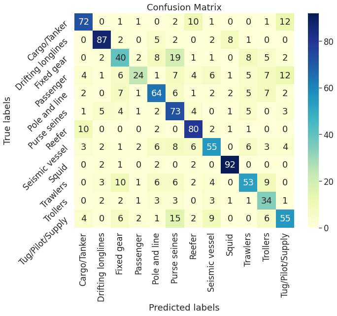
Figure 4: Confusion matrices for one 10-fold nested cross validation experiment on the vessel classification dataset. Left: KNN, Right: SVM

In Figure 4, we show the confusion matrices for both KNN and SVM for a fixed, illustrative run of 10-fold nested cross validation. Looking at the confusion matrices, we see that perhaps some mislabeling is warranted. In particular, we note three main types of mislabeling: fishing vessels getting labeled as other types of fishing vessels, reefers (refrigerated cargo) and cargo vessels getting confused, and tugboats getting confused with various classes. It is reasonable to expect that different types of fishing vessels may exhibit similar movement patterns; the same is true for reefers and cargo vessels. High confusion with tug/pilot/supply is also interesting but not surprising; a ship broken down at sea that requires a tugboat is likely to exhibit similar movement patterns to a tugboat.

Figure 5: Confusion matrices for one 10-fold nested cross validation experiment on the vessel classification dataset for the binary problem of whether a vessel is involved in fishing. Left: KNN, Right: SVM

To give some credence to our claim that mislabeling of one fishing vessel with another is reasonable, we also show in Figure 5 the confusion matrices for the binary classification problem of whether a vessel is involved in fishing. Here, the KNN model achieves an accuracy of 89.88% while the SVM model achieves an accuracy of 90.61%. Again, note that this is with a nested cross validation procedure on approximately two percent of the data available in [25], the model in which achieves a near-perfect accuracy score. This further supports that our features are accurately capturing quantities of interest.

7.5 Details of empirical studies

7.5.1 Individual windows

Table 6: Tables showing accuracy statistics for the UCR 2018 repository for models trained on the individual windows of a 6-window GeoStat representation.

Dataset (SVM)	Window 1	Window 2	Window 3	Window 4	Window 5	Window 6
ACSF1	0.6000	0.4860	0.4700	0.5800	0.5720	0.7200
Adiac	0.6552	0.5402	0.6496	0.6486	0.5995	0.6547
AllGestureWiimoteX	0.2486	0.3543	0.3871	0.3991	0.3371	0.3069
AllGestureWiimoteY	0.3271	0.3383	0.3786	0.3686	0.3251	0.3357
AllGestureWiimoteZ	0.2929	0.3037	0.3571	0.3429	0.3171	0.3080
ArrowHead	0.6000	0.7109	0.7143	0.7200	0.6377	0.5943
BME	0.6533	0.4413	0.3773	0.4293	0.5267	0.6747
Beef	0.7333	0.5333	0.6867	0.5800	0.4667	0.6133
BeetleFly	0.6900	0.8000	0.6500	0.6500	0.7500	0.8400
BirdChicken	0.7600	0.7000	0.9000	0.9500	0.7000	0.9500
CBF	0.5756	0.8522	0.7289	0.7222	0.6262	0.5467
Car	0.6833	0.6700	0.7167	0.6567	0.5633	0.5100
Chinatown	0.9125	0.8058	0.7114	0.7977	0.7743	0.5090
ChlorineConcentration	0.5953	0.6461	0.6089	0.5916	0.6883	0.6133
CinCECGTorso	0.5970	0.7533	0.6951	0.8275	0.7448	0.6197
Coffee	0.9143	0.8357	0.8071	0.9286	1.0000	0.8929
Computers	0.6624	0.7120	0.7040	0.6960	0.6440	0.6272
CricketX	0.2641	0.5256	0.4692	0.3590	0.2410	0.1487
CricketY	0.3949	0.5538	0.4462	0.3241	0.2774	0.2200
CricketZ	0.2641	0.5462	0.4821	0.3179	0.2308	0.1564
DiatomSizeReduction	0.9412	0.8431	0.9222	0.8856	0.8595	0.7712
DistalPhalanxOutlineAgeGroup	0.6691	0.6719	0.6835	0.7050	0.7554	0.7338
DistalPhalanxOutlineCorrect	0.7377	0.6710	0.7464	0.7464	0.6884	0.6681
DistalPhalanxTW	0.6129	0.5741	0.5770	0.6691	0.6676	0.6878
DodgerLoopDay	0.2525	0.3950	0.3300	0.2450	0.3275	0.2850
DodgerLoopGame	0.4783	0.5232	0.5000	0.4855	0.5783	0.8333
DodgerLoopWeekend	0.8768	0.9638	0.9638	0.6725	0.7652	0.5899
ECG200	0.8180	0.8120	0.8300	0.8000	0.8100	0.7700
ECG5000	0.9251	0.9139	0.8451	0.8269	0.9254	0.9352
ECGFiveDays	0.6202	0.6002	0.9377	0.7271	0.7909	0.9782
EOGHorizontalSignal	0.0773	0.2044	0.3702	0.2155	0.2039	0.2315
EOGVerticalSignal	0.0978	0.2514	0.2569	0.2105	0.1773	0.1298
Earthquakes	0.7482	0.7482	0.7482	0.7482	0.7482	0.7396
EthanolLevel	0.3064	0.3236	0.2784	0.2660	0.7372	0.5188
FaceAll	0.7763	0.6207	0.6320	0.5231	0.5414	0.4592
FaceFour	0.6886	0.7386	0.7159	0.7886	0.5295	0.3295
FacesUCR	0.4513	0.5971	0.5520	0.7102	0.6042	0.6112
FiftyWords	0.5068	0.4760	0.4681	0.4703	0.4923	0.4681
Fish	0.7749	0.7829	0.7463	0.7440	0.6640	0.3783
FordA	0.7583	0.7395	0.7644	0.7267	0.7414	0.7273
FordB	0.6210	0.6464	0.6457	0.6432	0.6148	0.6531
FreezerRegularTrain	0.9505	0.9933	0.8652	0.8747	0.8340	0.7932
FreezerSmallTrain	0.8902	0.9926	0.8920	0.8677	0.7177	0.7888
Fungi	0.1237	0.4570	0.7151	0.6667	0.3495	0.2849
GestureMidAirD1	0.2200	0.3892	0.3415	0.3400	0.3431	0.3031
GestureMidAirD2	0.2262	0.2846	0.2615	0.2600	0.2385	0.2277
GestureMidAirD3	0.1231	0.1754	0.1831	0.1646	0.1338	0.1754
GesturePebbleZ1	0.3442	0.5651	0.6395	0.6628	0.8384	0.6826
GesturePebbleZ2	0.3038	0.4975	0.5633	0.6114	0.7089	0.6481
GunPoint	0.6933	0.9400	0.7293	0.8173	0.9147	0.8467
GunPointAgeSpan	0.8741	0.9462	0.8703	0.8184	0.9253	0.8513
GunPointMaleVersusFemale	0.9272	0.9190	0.9652	0.9127	0.8468	0.8544
GunPointOldVersusYoung	0.9714	0.9740	0.9937	1.0000	0.9683	0.9663
Ham	0.6686	0.5524	0.6629	0.5257	0.6286	0.6419
HandOutlines	0.7146	0.9141	0.8486	0.7724	0.7405	0.6784
Haptics	0.3805	0.4123	0.3727	0.3831	0.3955	0.4312
Herring	0.6594	0.6281	0.5938	0.5938	0.5938	0.5281
HouseTwenty	0.9076	0.8941	0.9092	0.8252	0.6168	0.6571
InlineSkate	0.3982	0.2524	0.2727	0.2687	0.3131	0.4098
InsectEPGRegularTrain	1.0000	0.9839	0.9823	0.9807	0.9960	1.0000
InsectEPGSmallTrain	0.9157	1.0000	0.8835	0.9687	0.9558	0.9839
InsectWingbeatSound	0.4725	0.4313	0.4626	0.3715	0.3424	0.3104
ItalyPowerDemand	0.6200	0.8140	0.7794	0.8185	0.9504	0.9252
LargeKitchenAppliances	0.5136	0.5755	0.6133	0.5947	0.6027	0.5243
Lightning2	0.6164	0.5803	0.7344	0.6361	0.5410	0.6361
Lightning7	0.4164	0.5315	0.4849	0.5562	0.6137	0.5342
Mallat	0.5850	0.6493	0.5082	0.6098	0.6235	0.7224
Meat	0.9300	0.8667	0.9867	0.8300	0.9133	0.8000
MedicalImages	0.7271	0.5382	0.5566	0.5487	0.5737	0.5755
MelbournePedestrian	0.6103	0.8163	0.8115	0.7708	0.8115	0.6134
MiddlePhalanxOutlineAgeGroup	0.6039	0.5766	0.5909	0.5753	0.5792	0.6182
MiddlePhalanxOutlineCorrect	0.6564	0.6460	0.5828	0.7237	0.7443	0.7113
MiddlePhalanxTW	0.5455	0.5468	0.5974	0.5779	0.5610	0.5831
MixedShapesRegularTrain	0.9010	0.9131	0.8973	0.8942	0.9015	0.8907
MixedShapesSmallTrain	0.8246	0.8456	0.8355	0.8284	0.8285	0.8304
MoteStrain	0.8858	0.7663	0.6414	0.8043	0.8227	0.7534
NonInvasiveFetalECGThorax1	0.8588	0.5069	0.5954	0.3968	0.5812	0.7235
NonInvasiveFetalECGThorax2	0.8744	0.5348	0.6651	0.4928	0.6590	0.8132
OSULeaf	0.6405	0.6636	0.6372	0.6496	0.6802	0.7107
OliveOil	0.7867	0.9000	0.8600	0.8667	0.8000	0.7000
PLAID	0.5624	0.4317	0.4510	0.4872	0.4860	0.4935
PhalangesOutlinesCorrect	0.7086	0.6993	0.7133	0.7664	0.6900	0.6876
Phoneme	0.1398	0.2120	0.1963	0.1755	0.1685	0.1558
PickupGestureWiimoteZ	0.4000	0.4840	0.4040	0.4240	0.4960	0.2960
PigAirwayPressure	0.1106	0.1058	0.1154	0.0808	0.1250	0.1231
PigArtPressure	0.7644	0.6990	0.7212	0.6827	0.6846	0.6808
PigCVP	0.2163	0.2308	0.2644	0.2067	0.2788	0.1731
Plane	0.9905	0.9905	1.0000	1.0000	0.9733	0.9790
PowerCons	0.6967	0.7600	0.7522	0.8000	0.9900	0.8833
RefrigerationDevices	0.5200	0.4976	0.4613	0.4635	0.4773	0.4960
Rock	0.6200	0.5200	0.5040	0.5400	0.7280	0.7800
ScreenType	0.3413	0.3600	0.3515	0.4747	0.4533	0.4720
SemgHandGenderCh2	0.7107	0.7807	0.6697	0.7637	0.6700	0.6587
SemgHandMovementCh2	0.4627	0.4244	0.3578	0.3600	0.3831	0.3733
SemgHandSubjectCh2	0.5071	0.5067	0.4507	0.4938	0.4311	0.4173
ShakeGestureWiimoteZ	0.4000	0.6200	0.5920	0.5120	0.5680	0.5440
ShapeletSim	0.5556	0.5267	0.5222	0.4500	0.5444	0.5267
ShapesAll	0.6450	0.6500	0.5867	0.6350	0.6517	0.6600
SmallKitchenAppliances	0.7637	0.7483	0.7397	0.7227	0.7157	0.7093
SmoothSubspace	0.5987	0.7267	0.6547	0.7800	0.6280	0.6067
SonyAIBORobotSurface1	0.8802	0.7687	0.5324	0.5584	0.7278	0.7304
SonyAIBORobotSurface2	0.7400	0.8233	0.6751	0.7209	0.8361	0.7933
StarLightCurves	0.9530	0.9517	0.9149	0.9451	0.9329	0.9381
Strawberry	0.9054	0.9486	0.9405	0.9486	0.8465	0.8865
SwedishLeaf	0.8480	0.7488	0.7952	0.7904	0.7514	0.8400
Symbols	0.6834	0.8344	0.8133	0.8683	0.8613	0.7833
SyntheticControl	0.8500	0.7527	0.8000	0.8467	0.6693	0.8333
ToeSegmentation1	0.5237	0.6772	0.5860	0.6588	0.7061	0.6746
ToeSegmentation2	0.6969	0.6831	0.6292	0.5692	0.6462	0.5015
Trace	0.6500	0.6880	0.6600	0.7620	0.8100	0.5000
TwoLeadECG	0.7073	0.8999	0.9377	0.7858	0.7208	0.6653
TwoPatterns	0.3305	0.3895	0.4090	0.4357	0.5172	0.3995
UMD	0.6667	0.6417	0.5153	0.4653	0.5750	0.6042
UWaveGestureLibraryAll	0.7462	0.8143	0.7024	0.7083	0.7151	0.6493
UWaveGestureLibraryX	0.5168	0.6499	0.5952	0.5931	0.6200	0.5823
UWaveGestureLibraryY	0.4963	0.5860	0.5324	0.5338	0.5357	0.5248
UWaveGestureLibraryZ	0.5059	0.6228	0.5461	0.5561	0.5353	0.4997
Wafer	0.9924	0.9869	0.9401	0.9518	0.9839	0.9937
Wine	0.7481	0.6852	0.7889	0.6852	0.5000	0.5556
WordSynonyms	0.4326	0.4295	0.4075	0.4279	0.4577	0.4636
Worms	0.5870	0.5714	0.6883	0.5714	0.5455	0.6364
WormsTwoClass	0.6883	0.6286	0.7584	0.7273	0.7299	0.6701
Yoga	0.7713	0.7257	0.6193	0.7103	0.7407	0.8083

Dataset (KNN)	Window 1	Window 2	Window 3	Window 4	Window 5	Window 6
ACSF1	0.6160	0.4700	0.5900	0.6000	0.5600	0.7900
Adiac	0.5499	0.4972	0.5703	0.5678	0.5243	0.5473
AllGestureWiimoteX	0.2357	0.3414	0.3877	0.3757	0.3223	0.2780
AllGestureWiimoteY	0.2709	0.3489	0.3971	0.3720	0.3351	0.3429
AllGestureWiimoteZ	0.2966	0.3077	0.3471	0.3780	0.3300	0.2883
ArrowHead	0.5486	0.6971	0.7017	0.6903	0.5886	0.5829
BME	0.6973	0.4053	0.4400	0.4227	0.4653	0.6200
Beef	0.6800	0.3800	0.4867	0.5000	0.4933	0.5067
BeetleFly	0.7000	0.7000	0.5900	0.6000	0.8500	0.6600
BirdChicken	0.8500	0.8000	0.8500	0.7900	0.7000	0.8500
CBF	0.5758	0.8311	0.6576	0.7347	0.5989	0.5678
Car	0.7167	0.5367	0.6767	0.6567	0.5267	0.4800
Chinatown	0.9662	0.8484	0.7965	0.8222	0.6880	0.6636
ChlorineConcentration	0.5690	0.6199	0.5923	0.5698	0.6963	0.5968
CinCECGTorso	0.5732	0.6920	0.7428	0.8116	0.7122	0.6510
Coffee	0.7714	0.7857	0.7071	0.9571	1.0000	0.7929
Computers	0.6816	0.7008	0.7120	0.6664	0.6776	0.6496
CricketX	0.2641	0.5164	0.4092	0.3210	0.2082	0.1554
CricketY	0.3656	0.5615	0.4041	0.3549	0.2826	0.2221
CricketZ	0.2595	0.5621	0.4349	0.3672	0.2036	0.1405
DiatomSizeReduction	0.8922	0.7190	0.9118	0.8824	0.8268	0.7974
DistalPhalanxOutlineAgeGroup	0.6662	0.6590	0.6504	0.7137	0.7194	0.7122
DistalPhalanxOutlineCorrect	0.6572	0.6464	0.6986	0.7420	0.6551	0.6652
DistalPhalanxTW	0.5568	0.5554	0.5424	0.6374	0.6763	0.6388
DodgerLoopDay	0.2750	0.3750	0.3775	0.2375	0.2550	0.1750
DodgerLoopGame	0.5145	0.4913	0.4986	0.5217	0.5638	0.7899
DodgerLoopWeekend	0.8841	0.9783	0.9275	0.8058	0.7667	0.5710
ECG200	0.8400	0.8200	0.8300	0.7700	0.7280	0.7340
ECG5000	0.9268	0.9054	0.8063	0.8179	0.9220	0.9319
ECGFiveDays	0.6581	0.6490	0.8583	0.7415	0.7482	0.9129
EOGHorizontalSignal	0.0840	0.1906	0.3315	0.1994	0.2105	0.1796
EOGVerticalSignal	0.0657	0.2713	0.2414	0.1873	0.1282	0.1331
Earthquakes	0.7468	0.7410	0.7482	0.7410	0.7381	0.7511
EthanolLevel	0.2672	0.2980	0.3068	0.2484	0.5784	0.4168
FaceAll	0.6904	0.5781	0.6080	0.4770	0.4712	0.4021
FaceFour	0.5841	0.8068	0.7023	0.7409	0.4568	0.2841
FacesUCR	0.4126	0.5317	0.5307	0.6659	0.5433	0.5412
FiftyWords	0.4743	0.4642	0.4488	0.4440	0.4681	0.4602
Fish	0.7131	0.7714	0.7589	0.7486	0.5920	0.3749
FordA	0.6997	0.6950	0.7317	0.6974	0.7009	0.7029
FordB	0.6160	0.6412	0.6311	0.6504	0.6267	0.6299
FreezerRegularTrain	0.9502	0.9811	0.8722	0.8778	0.8512	0.7908
FreezerSmallTrain	0.8846	0.9639	0.9052	0.8606	0.7446	0.7182
Fungi	0.1344	0.4624	0.8065	0.7258	0.4194	0.3011
GestureMidAirD1	0.2308	0.3077	0.2738	0.3338	0.2892	0.2846
GestureMidAirD2	0.2169	0.2492	0.2385	0.2523	0.2400	0.2154
GestureMidAirD3	0.1231	0.2000	0.1646	0.1538	0.1585	0.1908
GesturePebbleZ1	0.3163	0.4198	0.5756	0.6372	0.7698	0.5640
GesturePebbleZ2	0.1949	0.3899	0.4380	0.5481	0.5696	0.5582
GunPoint	0.7693	0.9733	0.7627	0.8147	0.9067	0.8480
GunPointAgeSpan	0.8734	0.9772	0.8715	0.8576	0.9114	0.8778
GunPointMaleVersusFemale	0.9500	0.9563	0.9810	0.9329	0.8766	0.8785
GunPointOldVersusYoung	0.9841	0.9873	0.9905	0.9968	0.9778	0.9714
Ham	0.6457	0.5048	0.5429	0.5124	0.5981	0.4533
HandOutlines	0.7076	0.8443	0.7832	0.7578	0.7303	0.6422
Haptics	0.3558	0.3747	0.3714	0.3435	0.3948	0.4019
Herring	0.6094	0.5781	0.5719	0.5750	0.5844	0.5500
HouseTwenty	0.9328	0.9580	0.9076	0.8538	0.7513	0.6571
InlineSkate	0.4149	0.2658	0.2633	0.2945	0.3018	0.3742
InsectEPGRegularTrain	0.9454	0.9839	0.9783	0.9703	0.9703	0.9454
InsectEPGSmallTrain	0.9357	0.9116	0.9518	0.8618	0.9558	0.8353
InsectWingbeatSound	0.4468	0.4086	0.4016	0.3270	0.3102	0.2735
ItalyPowerDemand	0.6064	0.8091	0.8016	0.8148	0.9460	0.9333
LargeKitchenAppliances	0.5147	0.5083	0.6272	0.5947	0.5563	0.5733
Lightning2	0.5803	0.6131	0.7344	0.6393	0.7607	0.7180
Lightning7	0.4493	0.4219	0.4384	0.4932	0.6384	0.5041
Mallat	0.5267	0.6404	0.4289	0.5976	0.6792	0.6398
Meat	0.8933	0.8600	0.9967	0.8733	0.8967	0.8167
MedicalImages	0.6971	0.5421	0.5429	0.5316	0.5611	0.5776
MelbournePedestrian	0.5550	0.8073	0.8315	0.7847	0.7966	0.6113
MiddlePhalanxOutlineAgeGroup	0.5662	0.5455	0.5909	0.5545	0.6078	0.5584
MiddlePhalanxOutlineCorrect	0.6275	0.6742	0.5759	0.6866	0.7478	0.7182
MiddlePhalanxTW	0.5195	0.5052	0.5571	0.5623	0.5364	0.5286
MixedShapesRegularTrain	0.8831	0.9002	0.9037	0.8859	0.8721	0.8854
MixedShapesSmallTrain	0.7946	0.8130	0.8407	0.8099	0.8045	0.8118
MoteStrain	0.7542	0.8075	0.7196	0.7821	0.8395	0.7139
NonInvasiveFetalECGThorax1	0.7838	0.4208	0.4731	0.3351	0.4743	0.5999
NonInvasiveFetalECGThorax2	0.8490	0.4515	0.5410	0.4083	0.5641	0.7359
OSULeaf	0.6331	0.6025	0.6033	0.5711	0.6083	0.6256
OliveOil	0.7867	0.8467	0.7067	0.9133	0.8933	0.7000
PLAID	0.5996	0.5456	0.5903	0.5810	0.6387	0.5989
PhalangesOutlinesCorrect	0.6825	0.6811	0.6900	0.7354	0.6744	0.6783
Phoneme	0.1516	0.1646	0.1590	0.1826	0.1536	0.1373
PickupGestureWiimoteZ	0.4200	0.4400	0.3240	0.3560	0.3920	0.2960
PigAirwayPressure	0.1221	0.1144	0.1106	0.0817	0.1058	0.1250
PigArtPressure	0.7548	0.6875	0.7404	0.7115	0.7106	0.7067
PigCVP	0.2404	0.2837	0.2644	0.1971	0.3317	0.2212
Plane	0.9600	0.9810	0.9905	0.9905	0.9810	0.9714
PowerCons	0.7411	0.7556	0.7756	0.8100	0.9689	0.7978
RefrigerationDevices	0.5045	0.5120	0.5120	0.4661	0.4757	0.4693
Rock	0.7000	0.4080	0.6440	0.5160	0.8200	0.7600
ScreenType	0.4000	0.4053	0.3957	0.4821	0.4624	0.4880
SemgHandGenderCh2	0.7123	0.7750	0.6487	0.7407	0.6627	0.6930
SemgHandMovementCh2	0.4898	0.4618	0.3844	0.3707	0.3947	0.3862
SemgHandSubjectCh2	0.5387	0.5164	0.4236	0.4102	0.4387	0.4227
ShakeGestureWiimoteZ	0.4320	0.5800	0.5000	0.4360	0.5760	0.5200
ShapeletSim	0.5289	0.6056	0.5156	0.4633	0.5633	0.5333
ShapesAll	0.6377	0.6500	0.5817	0.6113	0.6583	0.6617
SmallKitchenAppliances	0.7184	0.7189	0.6661	0.6864	0.6757	0.6795
SmoothSubspace	0.6307	0.6907	0.6440	0.7573	0.6160	0.6107
SonyAIBORobotSurface1	0.8220	0.7864	0.4842	0.7238	0.6572	0.6998
SonyAIBORobotSurface2	0.7356	0.8520	0.7356	0.7051	0.8126	0.7859
StarLightCurves	0.9476	0.9520	0.9157	0.9377	0.9253	0.9323
Strawberry	0.8811	0.9703	0.9097	0.9514	0.8184	0.8865
SwedishLeaf	0.7920	0.7178	0.7568	0.7584	0.7251	0.7702
Symbols	0.6563	0.8462	0.8318	0.8804	0.8804	0.7337
SyntheticControl	0.7973	0.7153	0.7513	0.7793	0.6973	0.7187
ToeSegmentation1	0.5763	0.6474	0.6149	0.6640	0.6263	0.6184
ToeSegmentation2	0.7708	0.6385	0.6662	0.7569	0.6708	0.5462
Trace	0.5560	0.6900	0.6100	0.6920	0.7140	0.4720
TwoLeadECG	0.7152	0.7638	0.9284	0.6795	0.6681	0.5877
TwoPatterns	0.3327	0.3689	0.3858	0.4079	0.5154	0.4002
UMD	0.6681	0.6306	0.5528	0.4389	0.5722	0.6569
UWaveGestureLibraryAll	0.7267	0.7446	0.6524	0.6744	0.6887	0.5915
UWaveGestureLibraryX	0.5177	0.6424	0.5869	0.5728	0.6091	0.5824
UWaveGestureLibraryY	0.4784	0.5650	0.5260	0.5224	0.5176	0.5221
UWaveGestureLibraryZ	0.5034	0.6013	0.5503	0.5281	0.5181	0.4954
Wafer	0.9932	0.9914	0.9737	0.9724	0.9867	0.9950
Wine	0.5963	0.6222	0.7556	0.6296	0.4259	0.4963
WordSynonyms	0.4122	0.4245	0.4056	0.4088	0.4545	0.4580
Worms	0.6597	0.5922	0.6390	0.6857	0.5896	0.6442
WormsTwoClass	0.6961	0.6779	0.7299	0.7299	0.6649	0.6883
Yoga	0.7571	0.7417	0.6579	0.7353	0.7488	0.7919

Table 6 shows the accuracy of trained models on individual of a 6-window GeoStat representation. In this instance, one iteration of Laplacian smoothing was used. It is interesting to see that, despite the restriction

7.5.2 Parameter ablation

Table 7: Tables showing ablation results for both geometric features and types of statistics used on the UCR 2018 Repository. All categories listed are those delineated by the repository, and all results are given in percent difference in mean classification accuracy. The number of datasets in each category is given in parentheses.

Type	Position	Velocity	Acceleration	Absolute Curvature	Curvature	Both Curvatures	2nd Derivatives
Device (8)	-6.6283	-1.9901	-0.4986	0.1156	-0.2314	-1.2108	-2.5083
ECG (6)	-6.5011	-1.3558	0.6817	0.7456	0.8118	1.2130	0.6745
EOG (2)	-25.9504	-10.5079	8.4299	4.6013	2.2545	8.7351	22.2034
EPG (2)	-1.2097	-0.3219	0.0000	-0.0404	0.0000	-0.2018	-0.3632
Hemodynamics (3)	-18.3701	-1.8471	4.6612	0.5286	5.2521	2.7055	-5.3443
HRM (1)	-16.3793	-12.0690	0.8621	1.7241	6.0345	21.5517	18.1034
Image (32)	-6.4021	-2.4677	0.5646	0.3708	0.5704	0.6699	-2.4795
Motion (17)	-4.6946	-6.1551	1.1760	1.2263	0.7387	1.0527	0.5313
Power (1)	-9.2154	-1.8680	-1.1208	0.6227	0.8717	-0.3736	0.2491
Sensor (30)	-9.2032	-3.5468	-0.2810	0.6816	0.1681	0.6102	-1.0340
Simulated (8)	-5.9837	-11.9659	-0.9676	-0.2891	-0.4647	-0.7120	-1.1466
Spectro (8)	-11.4281	-4.8479	1.7865	1.2144	1.9862	4.3437	3.9833
Spectrum (4)	-3.4562	0.0684	-3.7223	2.3696	1.1979	1.9395	5.5012
Traffic (2)	-4.4758	0.1535	-1.8042	3.4192	2.5461	7.3729	10.2489
Trajectory (3)	-19.3763	-26.2705	-3.0396	-1.8606	0.0026	-4.8231	-0.1616

Type	Range	Mean	Standard Dev.	Skew	Kurtosis	Low Quantiles	Mid Quantiles	High Quantiles
Device (8)	0.1392	0.3857	-0.0477	-1.3060	-1.0224	-0.9925	-0.3265	-0.5970
ECG (6)	-1.3665	0.6297	-0.0333	0.2126	0.3076	-0.3893	-0.2882	-2.9651
EOG (2)	1.1941	0.8942	-0.0747	-6.9520	3.3519	2.0084	0.5363	6.2002
EPG (2)	0.0000	-0.0402	0.0000	0.0000	-0.0404	-0.2815	0.0404	-0.4843
Hemodynamics (3)	-0.9417	9.6946	-0.9543	-3.6998	-1.6135	-1.3052	-1.0642	-5.2498
HRM (1)	2.5862	5.1724	1.7241	-3.4483	-2.5862	-2.5862	-1.7241	-20.6897
Image (32)	0.0032	-0.1809	0.0252	0.5852	-0.2947	-0.5708	-1.2744	-0.6648
Motion (17)	-0.2531	0.0215	0.8291	-0.3244	0.0116	1.1145	1.0723	-1.8961
Power (1)	-0.6227	0.0000	-0.7472	0.2491	-0.2491	-2.7397	0.0000	-1.1208
Sensor (30)	-0.1480	-0.5348	-0.4493	-0.5928	-0.5939	-1.3257	-0.9714	-0.4599
Simulated (8)	-0.3423	-0.2726	-0.0676	-0.3923	0.2106	-0.6146	-0.8238	-0.9734
Spectro (8)	0.2273	1.8783	0.0441	-1.7729	-0.2518	-0.7108	-0.4232	-3.0456
Spectrum (4)	0.5050	-0.3957	0.3904	1.0963	2.0436	-2.6752	0.2037	-2.5931
Traffic (2)	-0.2102	0.6328	0.2574	1.2277	1.6080	-0.4095	0.1539	-0.0939
Trajectory (3)	-1.7541	-1.8419	-1.6562	2.6862	-1.7937	-6.7577	-1.9549	-1.4024

Table 7 lists ablation results for each of the categories in the UCR 2018 repository. All results are reported in percent difference of average classification accuracy for a KNN model trained on 1-window GeoStat representations with one iteration of Laplacian smoothing. Results for an SVM model with the same parameters are given in the Supplementary Material. Note that choice of number of windows may affect this, but we did not address this directly. Though some numbers are quite large in magnitude, it is important to note that some categories have few datasets and thus may not be representative of all problems. As noted in the main text, both position and velocity information, as well as those of extremal quantiles, appear vital to the success of our representation. The former are not surprising, while the latter presents an interesting direction for future work. The affect of the other quantities, however, appear to be dataset dependent.

Table 8: Ablation results for a fixed random seed on the GFW vessel dataset

Removed Features	KNN	Percent Change
None	0.6622	0.0000
Active Times	0.6793	2.5825
Inactive Times	0.6685	0.9511
Unknown Times	0.6820	2.9956
Location	0.6504	-1.7785
Speed	0.6278	-5.1897
Acceleration	0.6586	-0.5491
Smoothed Curvature	0.6892	4.0840
Rough Curvature	0.6847	3.4000
All Curvatures	0.6847	3.4062
All Second Derivatives	0.6811	2.8521
Distance to Port	0.6703	1.2232
Distance to Shore	0.6739	1.7649
Range	0.6793	2.5899
Mean	0.6676	0.8101
Std	0.6784	2.4439
Skew	0.6775	2.3104
Kurtosis	0.6793	2.5862
Low Quantiles	0.6567	-0.8324
Mid Quantiles	0.6450	-2.6023
High Quantiles	0.6929	4.6356

Removed Features	SVM	Percent Change
None	0.6956	0.0000
Active Times	0.6830	-1.8202
Inactive Times	0.7028	1.0349
Unknown Times	0.6865	-1.3057
Location	0.6532	-6.1011
Speed	0.6486	-6.7545
Acceleration	0.6883	-1.0478
Smoothed Curvature	0.6983	0.3826
Rough Curvature	0.7001	0.6440
All Curvatures	0.6757	-2.8622
All Second Derivatives	0.6766	-2.7374
Distance to Port	0.6848	-1.5588
Distance to Shore	0.6848	-1.5588
Range	0.7010	0.7782
Mean	0.6956	-0.0059
Std	0.6974	0.2578
Skew	0.6983	0.3874
Kurtosis	0.6992	0.5145
Low Quantiles	0.6739	-3.1235
Mid Quantiles	0.6549	-5.8550
High Quantiles	0.6974	0.02567

For the multivariate setting, Table 8 shows the average effect of the removal of different sets of parameters on the accuracy of both KNN and SVM classifiers for the features given in the GFW dataset. The average is taken over thirty iterations of the 10-fold nested cross-validation procedure. By low, high, and mid quantiles, we mean the lowest four, highest four, and middle three considered of those previously mentioned. The removal of both location (position), speed, and the middle quantiles negatively effect both classifiers. This is unsurprising as the information contained within these (the value of the time series, the rate of change of the time series, and the typical behavior of all quantities) is important basic information.

References

- [1] S. Aghabozorgi, A. S. Shirkhorshidi, and T. Y. Wah. Time-series clustering–a decade review. Information Systems, 53:16–38, 2015.
- [2] A. Bagnall and J. Lines. An experimental evaluation of nearest neighbour time series classification. arXiv preprint arXiv:1406.4757, 2014.
- [3] A. Bagnall, J. Lines, A. Bostrom, J. Large, and E. Keogh. The great time series classification bake off: a review and experimental evaluation of recent algorithmic advances. Data Mining and Knowledge Discovery, 31(3):606–660, 2017.
- [4] A. Bagnall, J. Lines, J. Hills, and A. Bostrom. Time-series classification with cote: the collective of transformation-based ensembles. IEEE Transactions on Knowledge and Data Engineering, 27(9):2522–2535, 2015.
- [5] M. G. Baydogan, G. Runger, and E. Tuv. A bag-of-features framework to classify time series. IEEE transactions on pattern analysis and machine intelligence, 35(11):2796–2802, 2013.
- [6] D. J. Berndt and J. Clifford. Using dynamic time warping to find patterns in time series. In KDD workshop, volume 10, pages 359–370. Seattle, WA, 1994.
- [7] J. Bian, D. Tian, Y. Tang, and D. Tao. Trajectory data classification: A review. ACM Transactions on Intelligent Systems and Technology (TIST), 10(4):1–34, 2019.
- [8] K. Boerder, N. A. Miller, and B. Worm. Global hot spots of transshipment of fish catch at sea. Science advances, 4(7):eaat7159, 2018.
- [9] G. E. Box, G. M. Jenkins, G. C. Reinsel, and G. M. Ljung. Time series analysis: forecasting and control. John Wiley & Sons, 2015.
- [10] M. Corduas and D. Piccolo. Time series clustering and classification by the autoregressive metric. Computational statistics & data analysis, 52(4):1860–1872, 2008.
- [11] Z. Cui, W. Chen, and Y. Chen. Multi-scale convolutional neural networks for time series classification. arXiv preprint arXiv:1603.06995, 2016.
- [12] H. A. Dau, A. Bagnall, K. Kamgar, C.-C. M. Yeh, Y. Zhu, S. Gharghabi, C. A. Ratanamahatana, and E. Keogh. The ucr time series archive. IEEE/CAA Journal of Automatica Sinica, 6(6):1293–1305, 2019.
- [13] H. Deng, G. Runger, E. Tuv, and M. Vladimir. A time series forest for classification and feature extraction. Information Sciences, 239:142–153, 2013.
- [14] M. P. Do Carmo. Differential geometry of curves and surfaces: revised and updated second edition. Courier Dover Publications, 2016.
- [15] M. Etemad, A. S. Júnior, and S. Matwin. Predicting transportation modes of gps trajectories using feature engineering and noise removal. In Canadian conference on artificial intelligence, pages 259–264. Springer, 2018.
- [16] H. Fawaz. Deep learning for time series classification. https://github.com/hfawaz/dl-4-tsc, 2019.
- [17] H. I. Fawaz, G. Forestier, J. Weber, L. Idoumghar, and P.-A. Muller. Deep learning for time series classification: a review. Data Mining and Knowledge Discovery, 33(4):917–963, 2019.
- [18] H. I. Fawaz, B. Lucas, G. Forestier, C. Pelletier, D. F. Schmidt, J. Weber, G. I. Webb, L. Idoumghar, P.-A. Muller, and F. Petitjean. Inceptiontime: Finding alexnet for time series classification. arXiv preprint arXiv:1909.04939, 2019.
- [19] T. Hastie, R. Tibshirani, and J. Friedman. The elements of statistical learning: data mining, inference, and prediction. Springer Science & Business Media, 2009.
- [20] K. He, X. Zhang, S. Ren, and J. Sun. Deep residual learning for image recognition. In Proceedings of the IEEE conference on computer vision and pattern recognition, pages 770–778, 2016.
- [21] J. Hills, J. Lines, E. Baranauskas, J. Mapp, and A. Bagnall. Classification of time series by shapelet transformation. Data Mining and Knowledge Discovery, 28(4):851–881, 2014.
- [22] Y.-S. Jeong, M. K. Jeong, and O. A. Omitaomu. Weighted dynamic time warping for time series classification. Pattern recognition, 44(9):2231–2240, 2011.
- [23] H. Karcher. Riemannian center of mass and mollifier smoothing. Communications on pure and applied mathematics, 30(5):509–541, 1977.
- [24] E. Keogh. Ucr time series classification archive. https://www.cs.ucr.edu/~eamonn/time_series_data_2018/, 2019.
- [25] D. A. Kroodsma, J. Mayorga, T. Hochberg, N. A. Miller, K. Boerder, F. Ferretti, A. Wilson, B. Bergman, T. D. White, B. A. Block, et al. Tracking the global footprint of fisheries. Science, 359(6378):904–908, 2018.
- [26] M. Kumar, N. R. Patel, and J. Woo. Clustering seasonality patterns in the presence of errors. In Proceedings of the eighth ACM SIGKDD international conference on Knowledge discovery and data mining, pages 557–563, 2002.
- [27] A. Le Guennec, S. Malinowski, and R. Tavenard. Data augmentation for time series classification using convolutional neural networks. In ECML/PKDD Workshop on Advanced Analytics and Learning on Temporal Data, 2016.
- [28] J. Lines, S. Taylor, and A. Bagnall. Hive-cote: The hierarchical vote collective of transformation-based ensembles for time series classification. In 2016 IEEE 16th international conference on data mining (ICDM), pages 1041–1046. IEEE, 2016.
- [29] C. H. Lubba, S. S. Sethi, P. Knaute, S. R. Schultz, B. D. Fulcher, and N. S. Jones. catch22: Canonical time-series characteristics. Data Mining and Knowledge Discovery, 33(6):1821–1852, 2019.
- [30] Q. Ma, J. Zheng, S. Li, and G. W. Cottrell. Learning representations for time series clustering. In Advances in Neural Information Processing Systems, pages 3776–3786, 2019.
- [31] J. D. Mazimpaka and S. Timpf. Trajectory data mining: A review of methods and applications. Journal of Spatial Information Science, 2016(13):61–99, 2016.
- [32] J. J. Rodríguez and C. J. Alonso. Support vector machines of interval-based features for time series classification. In International Conference on Innovative Techniques and Applications of Artificial Intelligence, pages 244–257. Springer, 2004.
- [33] P. Schäfer and U. Leser. Fast and accurate time series classification with weasel. In Proceedings of the 2017 ACM on Conference on Information and Knowledge Management, pages 637–646, 2017.
- [34] A. Shifaz, C. Pelletier, F. Petitjean, and G. I. Webb. Ts-chief: A scalable and accurate forest algorithm for time series classification. Data Mining and Knowledge Discovery, pages 1–34, 2020.
- [35] W. Song, L. Liu, M. Liu, W. Wang, X. Wang, and Y. Song. Representation learning with deconvolution for multivariate time series classification and visualization. In International Conference of Pioneering Computer Scientists, Engineers and Educators, pages 310–326. Springer, 2020.
- [36] M. D. Spivak. A comprehensive introduction to differential geometry. Publish or perish, 1970.
- [37] E. M. Stein and R. Shakarchi. Real analysis: measure theory, integration, and Hilbert spaces. Princeton University Press, 2009.
- [38] S. J. Taylor. Modelling financial time series. world scientific, 2008.
- [39] P. Virtanen, R. Gommers, T. E. Oliphant, M. Haberland, T. Reddy, D. Cournapeau, E. Burovski, P. Peterson, W. Weckesser, J. Bright, et al. Scipy 1.0: fundamental algorithms for scientific computing in python. Nature Methods, pages 1–12, 2020.
- [40] Z. Wang, W. Yan, and T. Oates. Time series classification from scratch with deep neural networks: A strong baseline. In 2017 International joint conference on neural networks (IJCNN), pages 1578–1585. IEEE, 2017.
- [41] G. F. Watch. Datasets and code. https://globalfishingwatch.org/datasets-and-code/ais-and-other-data/, 2017.
- [42] G. F. Watch. Training data. https://github.com/GlobalFishingWatch/training-data, 2017.
- [43] A. Wismüller, O. Lange, D. R. Dersch, G. L. Leinsinger, K. Hahn, B. Pütz, and D. Auer. Cluster analysis of biomedical image time-series. International Journal of Computer Vision, 46(2):103–128, 2002.
- [44] L. Ye and E. Keogh. Time series shapelets: a new primitive for data mining. In Proceedings of the 15th ACM SIGKDD international conference on Knowledge discovery and data mining, pages 947–956, 2009.
- [45] T. Zhang, H. Lu, and S. Z. Li. Learning semantic scene models by object classification and trajectory clustering. In 2009 IEEE conference on computer vision and pattern recognition, pages 1940–1947. IEEE, 2009.
- [46] B. Zhao, H. Lu, S. Chen, J. Liu, and D. Wu. Convolutional neural networks for time series classification. Journal of Systems Engineering and Electronics, 28(1):162–169, 2017.
- [47] B. Zhou, A. Khosla, A. Lapedriza, A. Oliva, and A. Torralba. Learning deep features for discriminative localization. In Proceedings of the IEEE conference on computer vision and pattern recognition, pages 2921–2929, 2016.