Benders decomposition for Network Design Covering Problems

Abstract

We consider two covering variants of the network design problem. We are given a set of origin/destination pairs, called O/D pairs, and each such O/D pair is covered if there exists a path in the network from the origin to the destination whose length is not larger than a given threshold. In the first problem, called the Maximal Covering Network Design problem, one must determine a network that maximizes the total fulfilled demand of the covered O/D pairs subject to a budget constraint on the design costs of the network. In the second problem, called the Partial Covering Network Design problem, the design cost is minimized while a lower bound is set on the total demand covered.
After presenting formulations, we develop a Benders decomposition approach to solve the problems. Further, we consider several stabilization methods to determine Benders cuts as well as the addition of cut-set inequalities to the master problem. We also consider the impact of adding an initial solution to our methods. Computational experiments show the efficiency of these different aspects.

1 Introduction

Network design is a broad and spread subject whose models often depend on the field in which they are applied. A classification of the basic problems of network design was done by Magnanti & Wong (1984) where some classical graph problems as the minimal spanning tree, Steiner tree, shortest path, facility location, and traveling salesman problems are included as particular cases of a general mathematical programming model. Since the construction of a network often costs large amount of money and time, decisions on network design are a crucial step when planning networks. Thus, network design is applied in a wide range of fields: transportation, telecommunication, energy, supply chain, geostatistics, evacuation, monitoring, etc. Infrastructure network design constitutes a major step in the planning of a transportation network since the performance, the efficiency, the robustness and other features strongly depend on the selected nodes and the way of connecting them, see Guihaire & Hao (2008). For instance, the main purpose of a rapid transit network is to improve the mobility of the inhabitants of a city or a metropolitan area. This improvement could lead to lower journey times, less pollution and/or less energy consumption which drives the communities to a more sustainable mobility.

Since it is generally too expensive to connect all the potential nodes, one must determine a subnetwork that serves at best the traffic demand. Depending on the application, different optimality measures can be considered. In particular, in the field of transportation, and especially in the area of passenger transportation, the aim is to get the infrastructure close to potential customers. In this framework, Schmidt & Schöbel (2014) propose to minimize the maximum routing cost for an origin-destination pair when using the new network. Alternatively, the traffic between an origin and a destination may be considered as captured if the cost or travel time when using the network is not larger than the cost or travel time of the best alternative solution (not using the new network). In this case, Perea et al. (2020) and García-Archilla et al. (2013) propose to select a sub(network) from an underlying network with the aim of capturing or covering as much traffic as possible for a reasonable construction cost. This paper is devoted to this problem, called the Maximum Covering Network Design Problem $(MC)$ as well as to the closely related problem called, Partial Covering Network Design Problem $(PC)$. The latter aims to minimize the network design cost for constructing the network under the constraint that a minimum percentage of the total traffic demand is covered.

Covering problems in graphs have attracted the attention of researchers since the middle of the last century. As far as the authors are aware the first papers on the vertex-covering problem were due to Berge (1957) and Norman & Rabin (1959) in the late 50s. This problem is related to the set-covering problem in which a family of sets is given and the minimal subfamily whose union contains all the elements is sought for. In Hakimi (1965) the vertex-covering problem was formulated as an integer linear programming model and solved by using Boolean functions. Toregas et al. (1971) applied the vertex-covering problem to the location of emergency services. They assumed that a vertex is covered if it is within a given coverage distance. Church & ReVelle (1974a) introduced the maximal covering location problem by fixing the number of facilities to be located. Each vertex has an associated population and the objective is to cover the maximum population within a fixed distance threshold. Since then many variants and extensions of the vertex-covering and maximal covering problems have been studied (see García & Marín (2020).)

When designing an infrastructure network, the demand is given by pairs of origin-destination points, called O/D pairs, and each such pair has an associated weight representing the traffic between the origin and the destination. Usually, this demand is encoded using an origin-destination matrix. When planning a new network, often there exists a network already functioning and offering its service to the same set of origin-destination pairs. For example, a new rapid transit system may be planned in order to improve the mobility of a big city or metropolitan area, in which there already exists another transit system, in addition to the private transportation system. This current transit system could be more dense than the planned one but slower since it uses the same right-of-way as the private traffic system. Thus, in some way both systems compete with each other and both compete with the private system of transportation. A similar effect occurs with mobile telecommunication operators. Therefore, the traffic between an origin and a destination is distributed among the several systems that provide the service.
There are mainly two ways of allocating the share of each system. The first one is the binary all-or-nothing way where the demand is only covered by one of the proposed modes. Typically, the demand is covered if the demand points are served within a range of quality service, as in Church & ReVelle (1974b). The second one is based on some continuous function, using, for example, a multi-logit probability distribution, as in Cascetta (2009). In this case, the demand is shared between the different systems. Both allocation schemes are based on the comparison of distances, times, costs, generalized costs or utilities. In this paper, we consider a binary one, where each O/D pair is covered only if the time spent to travel from its origin to its destination in the network is below a threshold. This threshold represents the comparison between the time spent in the proposed network and a private mode, assigning the full share to the most beneficial one.

Since most network design problems are NP-hard (see e.g. Perea et al. (2020)), recent research efforts have been oriented to apply metaheuristic algorithms to obtain good solutions in a reasonable computational time. Thus, in the field of transportation network design, Genetic Algorithms (Król & Król, 2019), Greedy Randomized Adaptive Search Procedures (García-Archilla et al., 2013), Adaptive Large Neighborhood Search Procedures (Canca et al., 2017) and Matheuristics (Canca et al., 2019) have been used to solve rapid transit network design problems and applied to medium-sized instances.

In this paper, after presenting models for problems $(MC)$ and $(PC)$, we propose exact methods based on Benders decomposition (Benders, 1962). This type of decomposition has been applied to many problems in different fields, see Rahmaniani et al. (2017) for a recent literature review on the use of Benders decomposition in combinatorial optimization. One recent contribution applied to set covering and maximal covering location problems appear in Cordeau et al. (2019). The authors propose different types of normalized Benders cuts for these two covering problems.

Benders decomposition for network design problems has been studied since the 80s. In Magnanti et al. (1986), the authors minimize the total construction cost of an uncapacitated network subject to the constraint that all O/D pairs must be covered. Given the structure of the problem, the Benders reformulation is stated with one subproblem for each O/D pair. A Benders decomposition for a multi-layer network design problem is presented in Fortz & Poss (2009). Benders decomposition was also applied in Botton et al. (2013) in the context of designing survivable networks. In Costa et al. (2009), a multi-commodity capacitated network design problem is studied and the strength of different Benders cuts is analysed. In Marín & Jaramillo (2009) a multi-objective approach is solved through Benders decomposition. The coverage is maximized and the total cost design is minimized. To the best of our knowledge, we apply for the first time a branch-and-Benders-cut approach to network design coverage problems. We also give a detailed study of some normalization techniques for Benders cuts in this context, including facet-defining cuts (Conforti & Wolsey, 2019). These cuts are a stronger version of the cuts proposed by Ben-Ameur & Neto (2007).

This paper presents several contributions. First, we present new mathematical integer formulations for the network design problems $(MC)$ and $(PC)$. The formulation for $(MC)$ is stronger than a previously proposed one, see e.g. Marín & Jaramillo (2009) and García-Archilla et al. (2013) (although the proposed formulation was not the main purpose of the latter), while $(PC)$ was never studied to the best of our knowledge. Our second contribution consists of polyhedral properties that are useful from the algorithmic point of view. A third contribution is the study of exact algorithms for the network design based on different Benders implementations. We propose a normalization technique and we consider the facet-defining cuts. Our computational experiments show that our Benders implementations are competitive with exact and non-exact methods existing in the literature and even comparing with the exact method of Benders decomposition existing in CPLEX.

The structure of the paper is as follows. In Section 2, we present mixed integer linear formulations for $(MC)$ and $(PC)$. We also study some polyhedral properties of the formulations and propose a simple algorithm to find an initial feasible solution for both problems. In Section 3, we study different Benders implementations and some algorithmic enhancements. Also, we discuss some improvements based on cut-set inequalities. A computational study is detailed in Section 4. Finally, our conclusions are presented in Section 5.

2 Problem formulations and some properties

In this section we present mixed integer linear formulations for the Maximal Covering Network Design Problem $(MC)$ and the Partial Set Covering Network Design Problem $(PC)$. We also describe some pre-processing methods and finish with some polyhedral properties. We first introduce some notation.

We consider an undirected graph denoted by $\mathcal{N}=(N,E)$, where $N$ and $E$ are the sets of potential nodes and edges that can be constructed. Each element $e\in E$ is denoted by $\{i,j\}$, with $i,j\in N$. We use the notation $i\in e$ if node $i$ is a terminal node of $e$. Let $\delta(i)$ be the set of edges incident to node $i$.

The mobility patterns are represented by a set $W\subset N\times N$ of O/D pairs. Each $w=(w^{s},w^{t})\in W$ is defined by an origin node $w^{s}\in N$, a destination node $w^{t}\in N$, an associated demand $g^{w}>0$ and a utility $u^{w}>0$. This utility translates the fact that there already exists a different network competing with the network to be constructed in an all-or-nothing way. In other words, an O/D pair $(w^{s},w^{t})$ will travel on the newly constructed network if it contains a path between $w^{s}$ and $w^{t}$ of length shorter than or equal to the utility $u^{w}$. We then say that the O/D pair is covered. In terms of the transportation area, the existing network represents a private transportation mode, the planned one represents a public transportation mode and the parameter $u^{w},\,w\in W$, refers to the utility of taking the private mode.

Costs for building nodes, $i\in N$, and edges, $e\in E$, are denoted by $b_{i}$ and $c_{e}$, respectively. The total construction cost cannot exceed the budget $C_{max}$. For example, in the context of constructing a transit network, each node cost may represent the total cost of building one station in a specific location in the network. On the other hand, each edge cost represents the total cost of linking two stations.

For each $e=\{i,j\}\in E$, we define two arcs: $a=(i,j)$ and $\hat{a}=(j,i)$. The resulting set of arcs is denoted by $A$. The length of arc $a\in A$ is denoted by $d_{a}$. For each O/D pair $w\in W$ we define a subgraph $\mathcal{N}^{w}=(N^{w},E^{w})$ containing all feasible nodes and edges for $w$, i.e. that belong to a path in $\mathcal{N}$ whose total length is lower than or equal to $u^{w}$. We also denote $A^{w}$ as the set of feasible arcs. In Section 2.2, we describe how to construct these subgraphs. We use notation $\delta_{w}^{+}(i)$ ($\delta_{w}^{-}(i)$ respectively) to denote the set of arcs going out (in respectively) of node $i\in N^{w}$. In particular, $\delta_{w}^{-}(w^{s})=\emptyset$ and $\delta_{w}^{+}(w^{t})=\emptyset$. We also denote by $\delta_{w}(i)$ the set of edges incident to node $i$ in graph $\mathcal{N}^{w}$.

2.1 Mixed Integer Linear Formulations

We first present a formulation of the Maximal Covering Network Design Problem $(MC)$, whose aim is to design an infrastructure network maximizing the total demand covered subject to a budget constraint:

$$(MC)\quad\max_{\boldsymbol{x},\boldsymbol{y},\boldsymbol{z},\boldsymbol{f}} \quad\sum_{w\in W}g^{w}z^{w}$$ (2.1)

s.t. $$\quad\sum_{e\in E}c_{e}x_{e}+\sum_{i\in N}b_{i}y_{i}\leq C_{max},$$ (2.2)

$$\quad x_{e}\leq y_{i},\hskip 227.62204pte\in E,i\in e,$$ (2.3)

$$\quad\sum_{a\in\delta_{w}^{+}(i)}f^{w}_{a}-\sum_{a\in\delta_{w}^{-}(i)}f^{w}_{a}=\begin{cases}z^{w},&\text{if $i=w^{s}$},\\ -z^{w},&\text{if $i=w^{t}$},\\ 0,&\text{otherwise},\end{cases}\hskip 51.21504ptw\in W,i\in N^{w},$$ (2.4)

$$\quad f^{w}_{a}+f^{w}_{\hat{a}}\leq x_{e},\hskip 56.9055ptw\in W,\,e=\{i,j\}\in E^{w}:a=(i,j),\,\hat{a}=(j,i),$$ (2.5)

$$\quad\sum_{a\in A^{w}}d_{a}f^{w}_{a}\leq u^{w}z^{w},\hskip 199.16928ptw\in W,$$ (2.6)

$$\quad y_{i},\,x_{e},\,z^{w}\in\{0,1\},\hskip 142.26378pti\in N,\,e\in E,\,w\in W,$$ (2.7)

$$\quad f_{a}^{w}\in\{0,1\},\hskip 199.16928pta\in A^{w},w\in W,$$ (2.8)

where $y_{i}$ and $x_{e}$ represent the binary design decisions of building node $i$ and edge $e$, respectively. Mode choice variable $z^{w}$ takes value $1$ if the O/D pair $w$ is covered and $0$ otherwise. Variables $f_{a}^{w}$ are used to model a path between $w^{s}$ and $w^{t}$, if possible. Variable $f_{a}^{w}$ takes value $1$ if arc $a$ belongs to the path from $w^{s}$ to $w^{t}$, and $0$ otherwise. Each variable $f^{w}_{a}$, such that $a\notin A^{w}$, is set to zero.

The objective function (2.1) to be maximized represents the demand covered. Constraint (2.2) limits the total construction cost. Constraint (2.3) ensures that if an edge is constructed, then its terminal nodes are constructed as well. For each pair $w$, expressions (2.4), (2.5) and (2.6) guarantee demand conservation and link flow variables $f_{a}^{w}$ with decision variables $z^{w}$ and design variables $x_{e}$. Constraints (2.5) are named capacity constraints and they force each edge to be used only in one direction at most. Constraints (2.6) referenced as mode choice constraints, put an upper bound on the length of the path for each pair $w$. This ensures variable $z^{w}$ to take value $1$ only if there exists a path between $w^{s}$ and $w^{t}$ with length at most $u^{w}$. This path is represented by variables $f_{a}^{w}$. Remark that several paths with length not larger than $u^{w}$ may exists for a given design solution $x,y$. Then, the values of the flow variables $f_{a}^{w}$ will describe one of them and the path choice has no influence on the objective function value (2.1). Finally, constraints (2.7) and (2.8) state that variables are binary.

The Partial Covering Network Design Problem $(PC)$, which minimizes the total construction cost of the network subject to a minimum coverage level of the total demand, can be formulated as follows:

$$(PC)\quad\min_{\boldsymbol{x},\boldsymbol{y},\boldsymbol{z},\boldsymbol{f}} \quad\sum_{i\in N}b_{i}y_{i}+\sum_{e\in E}c_{e}x_{e}$$ (2.9)

s.t. $$\quad\sum_{w\in W}g^{w}z^{w}\geq\beta\,G,$$ (2.10)

Constraints (2.3), (2.4), (2.5), (2.6), (2.7), (2.8),

where $\beta\in(0,1]$ and $G=\sum\limits_{w\in W}g^{w}$. Here, the objective function (2.9) to be minimized represents the design cost. Constraint (2.10) imposes that a proportion $\beta$ of the total demand is covered.

In the previous works by Marín & Jaramillo (2009) and García-Archilla et al. (2013), constraints (2.5) and (2.6) are formulated in a different way. For example, in García-Archilla et al. (2013), these constraints were written as

$$f_{a}^{w}+z^{w}-1\leq x_{a}, \kern-56.9055ptw\in W,\,e=\{i,j\}\in E^{w}:a=(i,j),$$ (2.11)

$$\sum_{a\in A^{w}}d_{a}f_{a}^{w}+M(z^{w}-1)\leq u^{w}z^{w}, w\in W,$$ (2.12)

where the design variable $x_{a}$ is defined for each arc. Given that $z^{w}-1\leq 0$, expressions (2.5) and (2.6) are stronger than (2.11) and (2.12), respectively.

In addition, constraint (2.12) involves a “big-M” constant. Our proposed formulation does not need it, which avoids the numerical instability generated by this constant. As we will see in Section 4.2, we observed that our proposed formulation is not only stronger than the one proposed in García-Archilla et al. (2013), but it is also computationally more efficient. In consequence, we only focus our analysis on our proposed formulation.

Another observation is that constraints (2.5) are a reinforcement of the usual capacity constraints $f_{a}^{w}\leq x_{e}$ and $f_{\hat{a}}^{w}\leq x_{e}$. In most applications where flow or design variables appear in the objective functions, the disaggregated version is sufficient to obtain a valid model as subtours are naturally non-optimal. However, it is not the case in our model, and there exist optimal solutions with subtours if the disaggregated version of (2.5) is used. Such a strengthening was already introduced in the context of uncapacitated network design, see e.g. Balakrishnan et al. (1989), and Steiner trees, see e.g. Sinnl & Ljubić (2016) and Fortz et al. (2021).

2.2 Pre-processing methods

In this section we describe some methods to reduce the size of the instances before solving them. First, we describe how to build each subgraph $\mathcal{N}^{w}=(N^{w},E^{w})$. Then for each problem, $(MC)$ and $(PC)$, we sketch a method to eliminate O/D pairs which will never be covered.

To create $\mathcal{N}^{w}$ we only consider useful nodes and edges from $\mathcal{N}$. For each O/D pair $w$, we eliminate all the nodes $i\in N$ that do not belong to any path from $w^{s}$ to $w^{t}$ shorter than $u^{w}$. Then, we define $E^{w}$ as the set of edges in $E$ incident only to the non eliminated nodes. Finally, the set $A^{w}$ is obtained by duplicating all edges in $E^{w}$ with the exception of arcs $(i,w^{s})$ and $(w^{t},i)$. We describe this procedure in Algorithm 1.

We assume that the cost of constructing each node and each edge is not higher than the budget.

Algorithm 1 Pre-processing I

  for $w\in W$ do

     $N^{w}=N$

     for $i\in N$ do

        compute the shortest path for the O/D pairs $(w^{s},i)$ and $(i,w^{t})$

        if the sum of the length of both paths is greater than $u^{w}$  then

           $N^{w}=N^{w}\setminus\{i\}$

           $E^{w}=E^{w}\setminus\delta(i)$

        end if

     end for

     $A^{w}=\{(i,j)\in A:\{i,j\}\in E^{w},\,j\neq w^{s},\,i\neq w^{t}\}$

  end for

  return  $\{\mathcal{N}^{w}=(N^{w},E^{w}),A^{w}\}_{w\in W}$

Next, we focus on $(MC)$. We can eliminate O/D pairs $w$ that are too expensive to be covered. That means, the O/D pair $w$ is deleted from $W$ if there is no path between $w^{s}$ and $w^{t}$ satisfying: i. its building cost is less than $C_{max}$; and ii. its length is less than $u^{w}$.
This can be checked by solving a shortest path problem with resource constraints and can thus be done in a pseudo-polynomial time. Desrochers (1986) shows how to adapt Bellman-Ford algorithm to solve it. However, given the moderate size of graphs we consider, we solve it as a feasibility problem. For each $w$, we consider the feasibility problem associated to constraints (2.2) (2.3), (2.4), (2.5), (2.6) and (2.7), with $z^{w}$ fixed to $1$. If this problem is infeasible, then the O/D pair $w$ is deleted from $W$. Otherwise, there exists a feasible path denoted by Path_w. We denote by $(\widetilde{N}^{w},\widetilde{E}^{w})$ the subgraph of $\mathcal{N}^{w}$ induced by Path_w.

2.3 Polyhedral properties

Both formulations $(MC)$ and $(PC)$ involve flow variables $f^{w}_{a}$ whose number can be huge when the number of O/D pairs is large. To circumvent this drawback we use a Benders decomposition approach for solving $(MC)$ and $(PC)$. In this subsection, we present properties of the two formulations that allow us to apply such a decomposition in an efficient way. The first proposition shows that we can relax the integrality constraints on the flow variables $f^{w}_{a}$. Let $(MC\_R)$ and $(PC\_R)$ denote the formulations $(MC)$ and $(PC)$ in which constraints (2.8) are replaced by non-negativity constraints, i.e.

$$f^{w}_{a}\geq 0,w\in W,a\in A.$$ (2.13)

We denote the set of feasible points to a formulation $F$ by $\mathcal{F}(F)$. Further, let $Q$ be a set of points $(\boldsymbol{x},\boldsymbol{z})\in R^{q}\times R^{p}$. Then the projection of $Q$ onto the $x$-space, denoted $Proj_{x}Q$, is the set of points given by $Proj_{\boldsymbol{x}}Q=\{\boldsymbol{x}\in R^{q}:(\boldsymbol{x},\boldsymbol{z})\in Q$ for some $\boldsymbol{z}\in R^{p}\}$.

Proposition 1.

$Proj_{\boldsymbol{x},\boldsymbol{y},\boldsymbol{z}}(\mathcal{F}(MC))=Proj_{\boldsymbol{x},\boldsymbol{y},\boldsymbol{z}}(\mathcal{F}(MC\_R))$ and $Proj_{\boldsymbol{x},\boldsymbol{y},\boldsymbol{z}}(\mathcal{F}(PC))=Proj_{\boldsymbol{x},\boldsymbol{y},\boldsymbol{z}}(\mathcal{F}(PC\_R))$.

Proof.

We provide the proof for $(MC)$, the other one being identical.

First, $\mathcal{F}(MC)\subseteq\mathcal{F}(MC\_R)$ implies $Proj_{\boldsymbol{x},\boldsymbol{y},\boldsymbol{z}}(\mathcal{F}(MC))\subseteq Proj_{\boldsymbol{x},\boldsymbol{y},\boldsymbol{z}}(\mathcal{F}(MC\_R))$. Second, let $(\boldsymbol{x},\boldsymbol{y},\boldsymbol{z})$ be a point belonging to $Proj_{\boldsymbol{x},\boldsymbol{y},\boldsymbol{z}}(\mathcal{F}(MC\_R))$. For every O/D pair $w\in W$ such that $z^{w}=0$ then $\boldsymbol{f}^{w}=0$. In the case where $z^{w}=1$, there exists a flow $f^{w}_{a}\geq 0$ satisfying (2.4) and (2.5) that can be decomposed into a convex combination of flows on paths from $w^{s}$ to $w^{t}$ and cycles. Given that the flow $f_{a}^{w}$ also satisfies (2.6), then a flow of value 1 on one of the paths in the convex combination must satisfy this constraint. Hence by taking $f_{a}^{w}$ equal to 1 for the arcs belonging to this path and to 0 otherwise, we show that $(\boldsymbol{x},\boldsymbol{y},\boldsymbol{z})$ also belongs to $Proj_{\boldsymbol{x},\boldsymbol{y},\boldsymbol{z}}(\mathcal{F}(MC))$. ∎

Note that a similar result is presented in the recent article Ljubić et al. (2019). Based on Proposition 1, we propose a Benders decomposition where variables $f^{w}_{a}$ are projected out from the model and replaced by Benders feasibility cuts. As we will see in Section 3.3, we also consider the Benders facet-defining cuts proposed in Conforti & Wolsey (2019). To apply this technique it is necessary to get an interior point of the convex hull of $Proj_{\boldsymbol{x},\boldsymbol{y},\boldsymbol{z}}(\mathcal{F}(MC\_R))$ (resp. $Proj_{\boldsymbol{x},\boldsymbol{y},\boldsymbol{z}}(\mathcal{F}(PC\_R))$). The following property gives us an algorithmic tool to apply this technique to $(MC)$.

Proposition 2.

After pre-processing, the convex hull of $Proj_{\boldsymbol{x},\boldsymbol{y},\boldsymbol{z}}(\mathcal{F}(MC\_R))$ is full-dimensional.

Proof.

To prove the result, we exhibit $|N|+|E|+|W|+1$ affinely independent feasible points:

• The $0$ vector is feasible.

• For each $i\in N$, the points:

  $$y_{i}=1,\,y_{i^{\prime}}=0,\,i^{\prime}\in N\setminus\{i\},\quad x_{e}=0,\,e\in E,\quad z^{w}=0,\,w\in W.$$

• For each $e=\{i,j\}\in E$, the points:

  $$y_{k}=1,\,k\in e,\,y_{k}=0,\,k\in N\setminus\{i,j\},\quad x_{e}=1,\,x_{e^{\prime}}=0,\,e^{\prime}\in E\setminus\{e\},\quad z^{w}=0,\,w\in W.$$

• For each $w\in W$, the points:

  $$y_{i}=1,\,i\in\widetilde{N}^{w},\,y_{i}=0,\,i\in N\setminus\widetilde{N}^{w},\quad x_{e}=1,\,e\in\widetilde{E}^{w},\,x_{e}=0,\,e\in E\setminus\widetilde{E}^{w},$$

  $$z^{w}=1,\,z^{w^{\prime}}=0,\,w^{\prime}\in W\setminus\{w\}.$$

Clearly these points are feasible and affinely independent. Thus the polytope is full-dimensional. ∎

The proof of Proposition 2 gives us a way to compute an interior point of the convex hull of $Proj_{\boldsymbol{x},\boldsymbol{y},\boldsymbol{z}}(\mathcal{F}(MC\_R))$. The average of these $|N|+|E|+|W|+1$ points is indeed such an interior point.

This is not the case for $(PC)$ as we show in Example $1$.

Example 1

Consider the instance of $(PC)$ given by the data presented in Table 1 and Figure 1. We consider the case where at least half of the population must be covered, that is $\beta=0.5$. In order to satisfy the trip coverage constraint (2.10), the O/D pair $w=(1,4)$ must be covered. Hence $z^{(1,4)}=1$ is an implicit equality. Furthermore, the only path with a length less than or equal to $u^{(1,4)}=15$ is composed of edges {1,2} and {2,4}. Hence, $x_{\{1,2\}}$, $x_{\{2,4\}}$, $y_{1}$, $y_{2}$ and $y_{4}$ must take value $1$. In consequence, the polytope associated to $(PC)$ is not full-dimensional.

Origin	Destination	$u^{w}$	$g^{w}$
1	4	15	200
2	4	10	50
3	4	15	50

Table 1: Data in Example 1. We consider $\beta=0.5$.

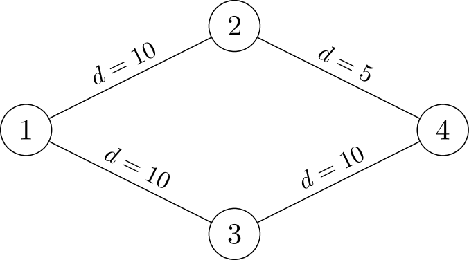
Figure 1: Graph of Example 1.

We can compute the dimension of the convex hull of $Proj_{\boldsymbol{x},\boldsymbol{y},\boldsymbol{z}}(\mathcal{F}(PC\_R))$ in an algorithmic fashion.

We find feasible affinely independent points and, at the same time, we detect O/D pairs which must be covered in any feasible solution. Due to the latter, there are a subset of nodes and a subset of edges that have to be built in any feasible solution. This means that there is a subset of design variables $y_{i},i\in N$, $x_{e},e\in E$ and mode choice variables $z^{w},w\in W$ that must take value $1$. At the opposite to $(MC)$, a solution to $(PC)$ with all variables set to $0$ is not feasible. However, the solution obtained by serving all O/D pairs and building all nodes and edges is feasible. Therefore, we start with a solution with all variables in $\boldsymbol{x},\boldsymbol{y},\boldsymbol{z}$ set to $1$ and we check, one by one, if it is feasible to set them to $0$. By setting one variable $x_{e}$ or $y_{i}$ to $0$, it may become impossible to cover some O/D pair $w$. In this case, we say that edge $e$ and node $i$ is essential for $w$. To simplify the notation, we introduce the binary parameters $\theta^{w}_{e}$ and $\theta^{w}_{i}$ taking value $1$ if edge $e$ (respectively node $i$) is essential for $w$. These new points are stored in a set $L$. Each time the algorithm finds a variable that cannot be set to $0$, we store it in sets $\bar{N},\,\bar{E},\,\bar{W}$, respectively. At the end of the algorithm, the dimension of the convex hull of $Proj_{\boldsymbol{x},\boldsymbol{y},\boldsymbol{z}}(\mathcal{F}(PC\_R))$ is

$$\dim(\mathcal{P}_{\boldsymbol{x},\boldsymbol{y},\boldsymbol{z}})=|N|+|E|+|W|-(|\bar{N}|+|\bar{E}|+|\bar{W}|).$$

This procedure is depicted in Algorithm 2.

Algorithm 2 Computing the dimension of the polytope of $(PC)$

  Initialization: Set $\bar{N}=\emptyset$, $\bar{E}=\emptyset$, $\bar{W}=\emptyset$ and $L=\emptyset$

  Add to set $L$: $\left(y_{i}=1,i\in N,\quad x_{e}=1,e\in E,\quad z^{w}=1,w\in W\right).$

  for $w^{\prime}\in W$ do

     if $\sum\limits_{w\in W\setminus\{w^{\prime}\}}g^{w}\geq\beta\,G$ then

        

        Add to set $L$: $\left(y_{i}=1,i\in N,\quad x_{e}=1,e\in E,\quad z^{w^{\prime}}=0,\,z^{w}=1,w\in W\setminus\{w^{\prime}\}\right).$

     else

        $\bar{W}=\bar{W}\cup\{w^{\prime}\}$

        for $e=\{i,j\}\in E$ do

           Compute shortest path between $w^{\prime s}$ and $w^{\prime t}$ in the graph $(N^{w^{\prime}},E^{w^{\prime}}\setminus\{e\})$.

           if the length of the shortest path is greater than $u^{w^{\prime}}$ or there is no path between $w^{\prime s}$ and $w^{\prime t}$ then

              $\bar{E}=\bar{E}\cup\{e\}$ and $\bar{N}=\bar{N}\cup\{i,j\}$

           end if

        end for

     end if

  end for

  for $e^{\prime}\in E\setminus\bar{E}$ do

     Add to set $L$: $\left(y_{i}=1,\,i\in N,\quad x_{e}=1,e\in E\setminus\{e^{\prime}\},x_{e^{\prime}}=0,\quad z^{w}=1-\theta^{w}_{e^{\prime}},w\in W\right).$

  end for

  for $i^{\prime}\in N\setminus\bar{N}$ do

     Add to set $L$: $\bigl{(}y_{i^{\prime}}=0,\,y_{i}=1,i\in N\setminus\{i^{\prime}\},\quad x_{e}=0,i^{\prime}\in e,\,x_{e}=1,i^{\prime}\notin e,\quad z^{w}=1-\theta^{w}_{i^{\prime}},w\in W\bigr{)}.$

  end for

  $\dim(\mathcal{P}_{\boldsymbol{x},\boldsymbol{y},\boldsymbol{z}})=|N|+|E|+|W|-(|\bar{N}|+|\bar{E}|+|\bar{W}|).$

  return  $\bar{N},\,\bar{E},\,\bar{W}$, $L$ and $\dim(conv(P_{\boldsymbol{x},\boldsymbol{y},\boldsymbol{z}}))$.

Algorithm 2 allows : i) to set some binary variables equal to $1$, decreasing the problem size; and ii) to compute a relative interior point of the convex hull of $Proj_{\boldsymbol{x},\boldsymbol{y},\boldsymbol{z}}(\mathcal{F}(PC\_R))$, necessary for the facet-defining cuts, as explained below in Section 3.3. The relative interior point is given by the average of the points in set $L$.

Example 1 cont

Regarding the previous example and following Algorithm 2, the O/D pair $(1,4)$ must be covered, $z^{(1,4)}=1$. Due to that, as its shortest path in the networks $(N^{(1,4)},E^{(1,4)}\setminus\{\{1,2\}\})$ and $(N^{(1,4)},E^{(1,4)}\setminus\{\{2,4\}\})$ is greater than $u^{(1,4)}=15$, variables $x_{\{1,2\}}$, $x_{\{2,4\}}$, $y_{1}$, $y_{2}$, $y_{4}$ are set to $1$. Finally, the dimension of this polyhedron is

$$\dim(P_{\boldsymbol{x},\boldsymbol{y},\boldsymbol{z}})=4+4+3-(3+2+1)=5.$$

The relative interior point computed is:

$$\,x_{\{1,2\}}=1,\,\,x_{\{2,4\}}=1,x_{\{1,3\}}=\frac{5}{6},\,x_{\{3,4\}}=\frac{2}{3},\,y_{1}=1,\,y_{2}=1,\,y_{3}=\frac{5}{6},\,y_{4}=\frac{5}{6},$$

$$z^{(1,4)}=1,\,z^{(2,4)}=\frac{5}{6},\,z^{(3,4)}=\frac{1}{2}.$$

2.4 Setting an initial solution

We determine an initial feasible solution for $(MC)$ and $(PC)$ with a simple greedy heuristic in which we sequentially select O/D pairs with best ratio demand overbuilding cost. More precisely, given the potential network $\mathcal{N}=(N,E)$, we compute for each O/D pair $w$ the ratio $r_{w}=\frac{g^{w}}{C(\mbox{Path}_{w})}$, where $C(\mbox{Path}_{w})$ is the cost of a feasible path for $w$. We order these ratios decreasingly. We use this initial order in the heuristic for both $(MC)$ and $(PC)$. For $(MC)$ the method proceeds as follows. It starts with an empty list of built nodes and edges, an empty list of O/D pairs covered, and a total cost set to $0$. For each O/D pair $w$, in decreasing order of $r_{w}$, the heuristic tries to build Path_w considering edges and nodes that are already built. If the additional cost plus the current cost is less than the budget $C_{max}$, nodes and edges in Path_w are built and the O/D pair $w$ is covered (i.e. $z^{w}=1$). The total cost, the lists of built nodes and edges are updated. Otherwise we proceed with the next O/D pair. At the end of the algorithm we have an initial feasible solution.

To get an initial solution for $(PC)$ we start with a list of all the O/D pairs covered and the amount of population covered equal to $G$. For each O/D pair $w$, in decreasing order of $r_{w}$, the algorithm checks if by deleting the O/D pair $w$ from the list, the coverage constraint (2.10) is satisfied. If so, the O/D pair $w$ is deleted from the list and the amount of population covered is updated. Finally, the algorithm builds the union of the subgraphs $(\widetilde{N}^{w},\widetilde{E}^{w})$ induced by Path_w for all the O/D pairs covered. Note that both initial solutions can be computed by solving $|W|$ shortest paths problems. These tasks can be executed much faster than solving $(MC)$ and $(PC)$ to optimality.

Pseudo-codes for both routines are provided in A. In Section 4, we will show the efficiency of adding this initial solution at the beginning of the branch-and-Benders-cut procedure.

3 Benders Implementations

In the following, we describe different Benders implementations for $(MC)$ and $(PC)$ obtained by projecting out variables $f^{w}_{a}$. Given that $(MC)$ and $(PC)$ share the same subproblem structure the Benders decomposition applied to $(MC)$ is valid for $(PC)$ and vice versa. Thus, we will apply the same Benders decomposition for both problems throughout this manuscript. These implementations are used as sub-routines in a branch-and-Benders-cut scheme. This scheme allows cutting infeasible solutions along the branch-and-bound tree. Depending on the implementation, infeasible solutions can be separated at any node in the branch-and-bound tree or only when an integer solution is found. In the case of $(MC)$, the master problem that we solve is:

$$(M\_MC)\quad\max\limits_{\boldsymbol{x},\boldsymbol{y},\boldsymbol{z}} \quad\sum_{w\in W}g^{w}z^{w}$$ (3.1)

s.t. (2.2),   (2.3),   (2.7)

$$\quad+\{\mbox{Benders Cuts }(\boldsymbol{x},\boldsymbol{y},\boldsymbol{z})\}.$$

The master problem for $(PC)$, named $(M\_PC)$, is stated analogously.

In Section 3.1, we discuss the standard Benders cuts obtained by dualizing the respective feasibility subproblem. Then, in Section 3.2 we discuss ways of generating normalized subproblems, to produce stronger cuts. We name these cuts normalized Benders cuts. In Section 3.3, we apply facet-defining cuts in order to get stronger cuts, as it is proposed in Conforti & Wolsey (2019). Finally, we discuss an implementation where, at the beginning, cut-set inequalities are added to enhance the link between $\boldsymbol{z}$ and $\boldsymbol{x}$, and then Benders cuts are added.

3.1 LP feasibility cuts

Since the structure of the model allows it, we consider a feasibility subproblem made of constraints (2.4), (2.5), (2.6) and (2.13) for each commodity $w\in W$, denoted by $(SP)^{w}$. We note that each subproblem is feasible whenever $z^{w}=0$, so it is necessary $(SP)^{w}$ to check feasibility only in the case where $z^{w}>0$. As it is clear from the context, we remove the index $w$ from the notation. The dual of each feasibility subproblem can be expressed as:

$$(DSP)^{w}\quad\max\limits_{\boldsymbol{\alpha},\boldsymbol{\sigma},\boldsymbol{\upsilon}} \quad z\,\alpha_{w^{s}}-\sum_{e\in E}x_{e}\,\sigma_{e}-u\,z\,\upsilon$$ (3.2)

s.t. $$\quad\alpha_{i}-\alpha_{j}-\sigma_{e}-d_{a}\,\upsilon\leq 0, a=(i,j)\in A:e=\{i,j\},$$ (3.3)

$$\quad\sigma_{e},\,\upsilon\geq 0, e\in E,$$ (3.4)

where $\boldsymbol{\alpha}$ is the vector of dual variables related to constraints (2.4), $\boldsymbol{\sigma}$ is the vector of dual variables corresponding to the set of constraints (2.5) and $\boldsymbol{\upsilon}$ is the dual variable of constraint (2.6). Since constraints in (2.4) are linearly dependent, we set $\alpha_{w^{t}}=0$. Given a solution of the master problem $(\boldsymbol{x},\boldsymbol{y},\boldsymbol{z})$, there are two possible outcomes for $(SP)^{w}$:

1. $(SP)^{w}$ is infeasible and $(DSP)^{w}$ is unbounded. Then, there exists an increasing direction $(\boldsymbol{\alpha},\boldsymbol{\sigma},\boldsymbol{\upsilon})$ with positive cost. In this case, the current solution $(\boldsymbol{x},\boldsymbol{y},\boldsymbol{z})$ is cut by:

   $$(\alpha_{w^{s}}-u\,\upsilon)\,z-\sum_{e\in E}\sigma_{e}\,x_{e}\leq 0.$$ (3.5)

2. $(SP)^{w}$ is feasible and consequently, $(DSP)^{w}$ has an optimal objective value equal to zero. In this case, no cut is added.

3.2 Normalized Benders cuts

The overall branch-and-Benders-cut performance heavily relies on how the cuts are implemented. It is known that feasibility cuts may have poor performance due to the lack of ability of selecting a good extreme ray (see for example Fischetti et al. (2010); Ljubić et al. (2012)). However, normalization techniques are known to be efficient to overcome this drawback Magnanti & Wong (1981); Balas & Perregaard (2002, 2003). The main idea is to transform extreme rays in extreme points of a suitable polytope. In this section we study three ways to normalize the dual subproblem described above.

First, we note that the feasibility subproblem can be reformulated as a min cost flow problem in $\mathcal{N}^{w}$ with capacities $\boldsymbol{x}$ and arc costs $d_{a}$.

$$(NSP)^{w}\quad\min\limits_{\boldsymbol{x},\boldsymbol{y},\boldsymbol{z},\boldsymbol{f}} \quad\sum_{a\in A}d_{a}\,f_{a}$$ (3.6)

s.t. (2.4), (2.5), (2.13).

The associated dual subproblem is:

$$(DNSP)^{w}\quad\max\limits_{\boldsymbol{\alpha},\boldsymbol{\sigma}} \quad z\,\alpha_{w^{s}}-\sum_{e\in E}\sigma_{e}x_{e}$$ (3.7)

s.t. $$\quad\alpha_{i}-\alpha_{j}-\sigma_{e}\leq d_{a}, a=(i,j)\in A:e=\{i,j\},$$ (3.8)

$$\quad\sigma_{e}\geq 0, e\in E.$$ (3.9)

Whenever $z^{w}>0$, the primal subproblem $(NSP)^{w}$ may be infeasible. Subproblems $(NSP)^{w}$ are no longer feasibility problems, although some of their respective dual forms can be unbounded. As the splitting demand constraint has to be satisfied there are two kind of cuts to add:

1. $(NSP)^{w}$ is infeasible and $(DNSP)^{w}$ is unbounded. In this case, the solution $(\boldsymbol{x},\boldsymbol{y},\boldsymbol{z})$ is cut by the constraint

   $$\alpha_{w^{s}}\,z-\sum\limits_{e\in E}\sigma_{e}\,x_{e}\leq 0.$$ (3.10)

2. $(NSP)^{w}$ is feasible and $(DNSP)^{w}$ has optimal solution. Consequently, if their solutions $(\boldsymbol{\alpha},\boldsymbol{\sigma})$ and $(\boldsymbol{x},\boldsymbol{y},\boldsymbol{z})$ satisfy that $\alpha_{w^{s}}\,z-\sum_{e\in E}\sigma_{e}\,x_{e}>u\,z$ then, the following cut is added

   $$(\alpha_{w^{s}}-u)\,z-\sum\limits_{e\in E}\sigma_{e}\,x_{e}\leq 0.$$ (3.11)

We refer to this implementation as BD_Norm1.

In this situation, there still exists dual subproblems $(DNSP)^{w}$ with extreme rays. We refer to BD_Norm2 as second dual normalization obtained by adding the dual constraint $\alpha_{w^{s}}=u+1$. In this case, every extreme ray of $(SP)^{w}$ corresponds to one of the extreme points of $(NSP)^{w}$. A cut is added whenever the optimal dual objective value is positive. This cut has the following form:

$$z-\sum_{e\in E}\sigma_{e}\,x_{e}\leq 0.$$ (3.12)

We finally tested a third dual normalization, BD_Norm3, by adding constraints

$$\sigma_{e}\leq 1,\qquad e\in E,$$ (3.13)

directly in $(DSP)^{w}$.

We tested the three dual normalizations described above for $(MC)$ using randomly generated networks with $10$, $20$ and $40$ nodes, as described in Subsection 4.1. As we will see in Section 4.2, only BD_Norm1 results to be competitive.

3.3 Facet-defining Benders cuts

Here we describe how to generate Benders cuts for $(MC)$ based on the ideas exposed in Conforti & Wolsey (2019), named as $CW$. The procedure for $(PC)$ is the same. Given an interior point or core point $(\boldsymbol{x}^{in},\boldsymbol{y}^{in},\boldsymbol{z}^{in})$ of the convex hull of feasible solutions and an exterior point $(\boldsymbol{x}^{out},\boldsymbol{y}^{out},\boldsymbol{z}^{out})$, that is a solution of the LP relaxation of the current restricted master problem, a cut that induces a facet or an improper face of the polyhedron defined by the LP relaxation of $Proj_{\boldsymbol{x},\boldsymbol{y},\boldsymbol{z}}\mathcal{F}(MC)$ is generated. We denote the difference $\boldsymbol{x}^{out}-\boldsymbol{x}^{in}$ by $\Delta\boldsymbol{x}$. We define $\Delta\boldsymbol{y}$ and $\Delta\boldsymbol{z}$ analogously. The idea is to find the furthest point from the core point, feasible to the LP-relaxation of $Proj_{\boldsymbol{x},\boldsymbol{y},\boldsymbol{z}}\mathcal{F}(MC)$ and lying on the segment line between the core point and the exterior point. This point is of the form $(\boldsymbol{x}^{sep},\boldsymbol{y}^{sep},\boldsymbol{z}^{sep})=(\boldsymbol{x}^{out},\boldsymbol{y}^{out},\boldsymbol{z}^{out})-\lambda(\Delta\boldsymbol{x},\Delta\boldsymbol{y},\Delta\boldsymbol{z})$. The problem of generating such a cut reads as follows:

$$(SP\_CW)^{w}\quad\min_{\boldsymbol{f},\lambda} \quad\lambda$$ (3.14)

s.t. $$\quad\sum_{a\in\delta_{w}^{+}(i)}f_{a}-\sum_{a\in\delta_{w}^{-}(i)}f_{a}=\begin{cases}z^{out}-\lambda\,\Delta z,&\text{if $i=w^{s}$,}\\ 0,&\text{otherwise,}\end{cases}$$ (3.15)

$$\quad f_{a}+f_{\hat{a}}\leq x^{out}_{e}-\lambda\,\Delta x_{e},\quad\qquad e=\{i,j\}\in E:a=(i,j),\hat{a}=(j,i),$$ (3.16)

$$\quad\sum_{a\in A}d_{a}\,f_{a}\leq u\,z^{out}-u\,\Delta z\,\lambda,$$ (3.17)

$$\quad 0\leq\lambda\leq 1,$$ (3.18)

$$\quad f_{a}\geq 0,\hskip 227.62204pta\in A.$$ (3.19)

In order to obtain the Benders feasibility cut we solve its associated dual:

$$(DSP\_CW)^{w}\quad\max_{\boldsymbol{\alpha},\boldsymbol{\sigma},\boldsymbol{\upsilon}} \quad z^{out}\,\alpha_{w^{s}}-\sum_{e\in E}x^{out}_{e}\,\sigma_{e}-u\,z^{out}\,\upsilon$$ (3.20)

s.t. $$\quad\Delta z\,\alpha_{w^{s}}-\sum_{e\in E}\Delta x_{e}\,\sigma_{e}-u\,\Delta z\,\upsilon\leq 1,$$ (3.21)

$$\quad\alpha_{i}-\alpha_{j}-\sigma_{e}-d_{a}\,\upsilon\leq 0,\qquad\qquad\quad a=(i,j)\in A:e=\{i,j\},$$

$$\quad\sigma_{e},\,\upsilon\geq 0,\hskip 196.32384pte\in E.$$

Given that $(SP\_CW)^{w}$ is always feasible ($\lambda=1$ is feasible) and that its optimal value is lower bounded by 0, then, both $(SP\_CW)^{w}$ and $(DSP\_CW)^{w}$ have always finite optimal solutions. Whenever the optimal value of $\lambda$ is 0, $(\boldsymbol{x}^{out},\boldsymbol{y}^{out},\boldsymbol{z}^{out})$ is feasible. A cut is added if the optimal value of $(DSP\_CW)^{w}$ is strictly greater than 0. The new cut has the same form as in (3.5). Note that this problem can be seen as a dual normalized version of $(SP)^{w}$ with the dual constraint (3.21). This approach is an improvement in comparison with the stabilization cuts proposed by Ben-Ameur & Neto (2007), where $\lambda$ is a fixed parameter.

Core points for both formulations can be obtained by computing the average of the points described in the proof of Proposition 2 for $(MC)$ and the average of the points in list $L$ obtained by applying Algorithm 2.

3.4 Cut-set inequalities

By projecting out variable vector $\boldsymbol{f}$, information regarding the link between vectors $\boldsymbol{x}$ and $\boldsymbol{z}$ is lost. Cut-set inequalities represent the information lost regarding the connectivity for the O/D pair $w$ in the solution given by the design variable vector $\boldsymbol{x}$. Let $(S,S^{C})$ be a $(w^{s},w^{t})$-partition of $N^{w}$ for a fixed O/D pair $w$, i.e. $(S,S^{C})$ satisfies: i. $w^{s}\in S$; ii. $w^{t}\in S^{C}$, with $S^{C}=N\setminus S$ its complement. A cut-set inequalities is defined as

$$z^{w}\leq\sum_{\begin{subarray}{c}\{i,j\}\in E^{w}:\\ i\in S,\,j\in S^{C}\end{subarray}}x_{\{i,j\}},\quad w\in W,\quad(S,S^{C})\mbox{ a }(w^{s},w^{t})\mbox{-partition of }N^{w}.$$ (3.22)

This type of constraints has been studied in several articles, for instance Barahona (1996); Koster et al. (2013); Costa et al. (2009). Note that it is easy to see that cut-set inequalities belong to the LP-based Benders family. Let $(S,S^{C})$ be a $(w^{s},w^{t})$-partition in the graph $\mathcal{N}^{w}$ for $w\in W$. Consider the following dual solution:

• $\alpha_{i}=1$ if $i\in S$; $\alpha_{i}=0$ if $i\in S^{C}$.

• $\sigma_{e}=1$ if $e=\{i,j\}\in E^{w}$, $i\in S$, $j\in S^{C}$; $\sigma_{e}=0$, otherwise.

• $\upsilon=0$.

This solution is feasible to $(DSP)^{w}$ and induces a cut as in (3.22). In order to improve computational performance, we test two approaches to include these inequalities:

1. We implement a modification of the Benders callback algorithm with the following idea. First, for each $w\in W$, using the solution vector $(\boldsymbol{x},\boldsymbol{y})$ from the master, the algorithm generates a network $(N^{w},E^{w})$ with capacity $1$ for each edge built. Then, a Depth-First Search (DFS) algorithm is applied to obtain the connected component containing $w^{s}$. If the connected component does not contain $w^{t}$, a cut of the form (3.22) is added. Otherwise, we generate a Benders cut as before. This routine is depicted in Algorithm 3.

   Algorithm 3 Callback implementation with cut-set inequalities.

   0:  ($x_{e},e\in E$, $z^{w},w\in W$) from the master solution solution $(\boldsymbol{x},\boldsymbol{y},\boldsymbol{z})$.

     for $w\in W$ do

        Build graph $(N^{w}({\boldsymbol{x}}),E^{w}({\boldsymbol{x}}))$ induced by the solution vector $\boldsymbol{x}$ from the master.

        Compute the connected component $S$ in $(N^{w}({\boldsymbol{x}}),E^{w}({\boldsymbol{x}}))$ containing $w^{s}$.

        if $w^{t}$ is not included in $S$ then

           Add the cut $z^{w}\leq\sum_{\begin{subarray}{c}\{i,j\}\in E^{w}:\\ i\in S,\,j\in S^{C}\end{subarray}}x_{\{i,j\}}$

        else

           Solve the corresponding subproblem ($(DSP)^{w}$, $(DNSP)^{w}$, $(DSP\_CW)^{w}$) and add cut if it is necessary.

        end if

     end for

     return  Cut.

   We tested this implementation with subproblems $(DSP\_CW)^{w}$. We observe that by using Algorithm 3 with $CW$ the convergence is slower and we generate more cuts. These preliminary results are shown in Table 5.

2. We add to the Master Problem the cut-set inequalities at the origin and at the destination of each O/D pair $w\in W$ at the beginning of the algorithm. These valid inequalities have the form:

   $$\begin{cases}z^{w}\leq\sum\limits_{e\in\delta(w^{s})}x_{e},\\ z^{w}\leq\sum\limits_{e\in\delta(w^{t})}x_{e}.\end{cases}$$ (3.23)

   This means that for each O/D pair to be covered, there should exist at least one edge incident to its origin and one edge incident to its destination, i.e. each O/D pair should have at least one arc going out of its origin and another one coming in its destination.

4 Computational Results

In this section, we compare the performance of the different families of Benders cuts presented in Section 3 using the branch-and-Benders-cut algorithm (denoted as B&BC).

All our computational experiments were performed on a computer equipped with a Intel Core i$5$-$7300$ CPU processor, with $2.50$ gigahertz $4$-core, and $16$ gigabytes of RAM memory. The operating system is $64$-bit Windows $10$. Codes were implemented in Python 3.8. These experiments have been carried out through CPLEX 12.10 solver, named CPLEX, using its Python interface. CPLEX parameters were set to their default values and the models were optimized in a single threaded mode.

For that, t denotes the average value for solution times given in seconds, gap denotes the average of relative optimality gaps in percent (the relative percent difference between the best solution and the best bound obtained within the time limit), LP gap denotes the average of LP gaps in percent and cuts is the average of number of cuts generated.

4.1 Data sets: benchmark networks and random instances

We divide the tested instances into two groups: benchmarks instances and random instances. Our benchmarks instances are composed by the Sevilla (García-Archilla et al., 2013) and Sioux Falls networks (Hellman, 2013).

The Sevilla instance is composed partially by the real data given by the authors of García-Archilla et al. (2013). From this data, we have used the topology of the underlying network, cost and distance vector for the set of arcs and the demand matrix. This network is composed of $49$ nodes and $119$ edges. Originally, the set of O/D pairs $W$ was formed by all possible ones ($49\cdot 48=2352$). However, some entries in the demand matrix of this instance are equal to 0 and we thus exclude them from the analysis. Specifically, $630$ pairs have zero demand, almost the $27\%$ of the whole set. We consider a private utility $u$ equal to twice the shortest path length in the underlying network. Each node cost is generated according to a uniform distribution $\mathcal{U}(7,13)$. The available budget has been fixed to $30\%$ of the cost of building the whole underlying network and the minimum proportion of demand to be covered to $\beta=0.5$.

For the Sioux Falls instance, the topology of the network is described by $24$ nodes and $38$ edges. Set $W$ is also formed by all possible O/D pairs ($38\cdot 37=1406$). The parameters have been chosen in the same manner as for the random instances.

We generate our random instances as follows. We consider planar networks with a set of $n$ nodes, with $n\in\{10,20,40,60\}$. Nodes are placed in a grid of $n$ square cells, each one of $10$ units side. For each cell, a point is randomly generated close to the center of the cell. For each setting of nodes we consider a planar graph with its maximum number of edges, deleting each edge with probability 0.3. We replicated this procedure $10$ times for each $n$, so that the number of nodes is the same while the number of edges may vary. Therefore, there are $40$ different underlying networks. We name these instances as $N10$, $N20$, $N40$ and $N60$. We provide the average cycle availability, connectivity and density for random instances networks in Table 2. A couple of them are depicted in Figure 2.

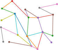
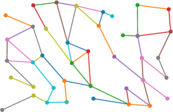
Figure 2: Example of underlying networks with $|N|$=20 and $|N|$=40.

Network	Cycle availability	Connectivity	Density
	$\frac{|E|-|N|+1}{2|N|-5}$	$\frac{|E|}{|N|}$	$\frac{|E|}{3(|N|-2)}$
N10	$0.11$	$1.05$	$0.44$
N20	$0.11$	$1.12$	$0.41$
N40	$0.13$	$1.22$	$0.43$
N60	$0.16$	$1.29$	$0.45$
Overall	$0.12$	$1.17$	$0.43$

Table 2: Cycle availability, connectivity and density parameters for the underlying networks in random instances.

Construction costs $b_{i}$, $i\in N$, are randomly generated according to a uniform distribution $\mathcal{U}(7,13)$. So, each node costs 10 monetary units in average. Construction cost of each edge $e\in E$, $c_{e}$, is set to its Euclidean length. This means that building the links cost 1 monetary unit per length unit. The node and edge costs are rounded to integer numbers. We set $C_{max}$ equal to $50\%$ of the cost of building the whole underlying network considered. We denote this total cost as $TC$, so $C_{max}=0.5\,TC$.

To build set $W$, we randomly pick each possible O/D pair of nodes with probability 0.5. In consequence, this set has $\frac{n(n-1)}{2}$ pairs in average. Parameter $u^{w}$ is set to 2 times the length of the shortest path between $w^{s}$ and $w^{t}$, named as $SPath^{w}$. Finally, the demand $g^{w}$ for each O/D pair $w$ is randomly generated according to the uniform distribution $\mathcal{U}(10,300)$.

4.2 Preliminary experiments

Before presenting an extensive computational study of the algorithms, we provide some preliminary results to: i. analyze the efficiency of the formulation presented in García-Archilla et al. (2013); ii. the efficiency of the cut normalizations described in Section 3.2 and, iii. the performance of the cut-set based Branch-and-cut procedure described in Section 3.4.

We first show that our formulation using (2.5)-(2.6) is not only stronger than the one formulated with (2.11)-(2.12) but also more efficient. Table 3 shows some statistics for the two formulations discussed at the end of Section 2.1, for instances with 10 and 20 nodes. We also tested instances with 40 nodes but most of them were not solved to optimality within one hour. In that case, we provide the optimality gap instead of the solution time. We consider 5 instances of each size. Note that constraints (2.12) are equivalent to constraints (2.6) by setting $M=0$. We tested several positive values for $M$.

Network	Formulation using (2.5)-(2.6)		Formulation using (2.11)-(2.12)
	t	LP gap	t	LP gap
N10	0.17	43.21	0.26	96.43
N20	5.78	56.33	228.22	106.71
	gap	LP gap	gap	LP gap
N40	11.74	68.15	54.85	137.13

Table 3: Comparing the performance of the two different types of mode choice and capacity constraints for $(MC)$ within a time limit of 1 hour. The majority of N40 instances were not solved to optimality, then the average gap is shown.

Secondly, we tested the three dual normalizations described in Section 3.2 for $(MC)$. Table 4 shows average values obtained for solution time in seconds and number of cuts needed for this experiment. The only one that seems competitive is BD_Norm1. We observed that cut coefficients generated with BD_Norm1 are mainly 0’s or 1’s. In the case of BD_Norm2 and BD_Norm3 we observe that coefficients generated are larger than the ones generated by BD_Norm1, so they may induce numerical instability. This situation is similar for the case of $(PC)$.

Network	BD_Norm1		BD_Norm2		BD_Norm3
	t	cuts	t	cuts	t	cuts
N10	0.21	44	0.22	47	0.24	104
N20	2.83	362	5.76	595	5.22	1418
N40	687.88	2904	*	*	*	*

Table 4: Comparing the performance of the three dual normalizations within a time limit of 1 hour for $(MC)$. N10, N20 and N40 are refereed to networks with 10, 20 and 40 nodes, respectively. The mark ’*’ indicates that four over five instances were not solved within 1 hour.

Finally, we tested the cut-set inequalities implementation described in Section 3.4 with subproblems $(DSP\_CW)^{w}$. We observe that by using Algorithm 3 with $CW$ the convergence is slower and we generate more cuts. This might be due to the fact that these cuts do not include information about the length of the path in the graph, but only information regarding the existence of the path. These preliminary results are shown in Table 5, which provides average values obtained for solution times in seconds and the number of cuts added.

Network	BD_CW		Algorithm 3+BD_CW
	t	cuts	t	cuts
N10	0.23	48	0.15	46
N20	2.47	411	2.53	500
N40	619.31	3486	722.02	3554

Table 5: Comparing the performance of the Algorithm 3 for $(MC)$. N10, N20 and N40 refer to networks with 10, 20 and 40 nodes respectively.

In conclusion, all these three implementations, with the exception of BD_norm1, are excluded from further analysis.

4.3 Branch-and-Benders-cut performance

Our preliminary experiments show that including cuts only at integer nodes of the branch and bound tree is more efficient than including them in nodes with fractional solutions. Thus, in our experiments we only separate integer solutions unless we specify the opposite. We used the LazyConstraintCallback function of CPLEX to separate integer solutions. Fractional solutions were separated using the UserCutCallback function. We study the different implementations of B&BC proposed in Sections 3.1, 3.2 and 3.3. We use the following nomenclature:

• BD_Trd: B&BC algorithm using the feasibility subproblems structure $(DSP)^{w}$, and its corresponding feasibility cuts (3.5).

• BD_Norm: B&BC algorithm using the normalized subproblems structure $(DNSP)^{w}$, and its corresponding cuts (3.10) and (3.11).

• BD_CW: B&BC algorithm using the subproblems structure $(DSP\_CW)^{w}$, and feasibility cuts (3.5).

We compare our algorithms with the direct use of CPLEX, and the automatic Benders procedure proposed by CPLEX, noted by AUTO_BD. CPLEX provides different implementations depending on the information that the user provides to the solver: i. CPLEX attempts to decompose the model strictly according to the decomposition provided by the user; ii. CPLEX decomposes the model by using this information as a hint and then refines the decomposition whenever possible; iii. CPLEX automatically decomposes the model, ignoring any information supplied by the user. We have tested these three possible settings, and only the first one is competitive.

Furthermore we have tested the following features:

• CS: If we include cut-set inequalities at each origin and destination as in (3.23).

• IS: If we provide an initial solution to the solver.

• RNC: If we add Benders cuts at the root node.

4.4 Performance of the algorithms on random instances

All the experiments have been performed with a limit of one hour of CPU time considering $10$ instances of each size. Tables in this section show average values obtained for solution times in seconds, relative gaps in percent, and number of cuts needed. To determine these averages, we only consider the instances solved at optimality by all the algorithms.

First, we compare the performance of CPLEX for formulations $(MC)$ and $(PC)$ and the three different B&BC implementations described above (BD_Trd, BD_Norm and BD_CW). We also study the impact of the initial cut set inequalities (CS) in the efficiency of the proposed algorithms. Table 6 shows the performance of the algorithms for networks N10, N20 and N40. All the algorithms are able to solve at optimality N10 and N20 instances in less than 7 seconds for $(MC)$ and $(PC)$. For $(MC)$ without CS, the fastest algorithm is BD_CW in sets N10, N20 and N40 for the instances solved at optimality. This is not the case for $(PC)$, since we can observe that AUTO_BD is slightly faster. In general, when CS is included, the solution time and the amount of cuts required decrease. Specifically, for $(MC)$ in N40, the most efficient algorithm is BD_CW+CS which gets the optimal solution $43.8\%$ faster than Auto_BD+CS. For $(PC)$, it seems to be also profitable, since for N40 BD_CW+CS gets the optimal solution using $55\%$ less time than Auto_BD. These results are shown in the second and fourth block of Table 6.

		Network	CPLEX	Auto_BD		BD_Trd		BD_Norm		BD_CW
			t	t	cuts	t	cuts	t	cuts	t	cuts
$(MC)$	w.o. CS	N10	0.18	0.43	27	0.25	92	0.24	91	0.19	94
		N20	6.77	4.51	273	3.89	620	3.18	590	3.34	641
		N40	1646.93	617.85	1967	1095.25	3990	541.03	3677	457.81	4137
	+CS	N10	-	0.32	12	0.21	49	0.28	52	0.23	54
		N20	-	3.94	178	2.29	382	2.50	383	1.85	416
		N40	-	484.95	1248	637.49	2378	575.87	2530	272.39	3186
$(PC)$	w.o. CS	N10	0.18	0.29	16	0.24	92	0.28	89	0.20	91
		N20	6.73	4.87	305	3.55	607	4.68	681	2.15	606
		N40	2153.15	504.06	1752	657.59	4470	514.42	4246	837.41	4412
	+CS	N10	-	0.28	11	0.16	56	0.20	57	0.145	54
		N20	-	4.12	213	3.11	497	3.43	495	2.070	461
		N40	-	439.23	1527	261.74	3528	323.21	3583	197.55	3949

Table 6: Comparing the performance of the three algorithms for $(MC)$ and $(PC)$.

Table 7 shows the instances in N40 solved in one hour. Without CS, some instances in set N40 cannot be solved to optimality neither for $(MC)$ nor for $(PC)$. Nevertheless, by including CS, Benders implementations can solve all the instances in N40 in the one hour limit.

		CPLEX	Auto_BD	BD_Trd	BD_Norm	BD_CW
$(MC)$	without CS	3	10	9	8	8
	+CS	-	10	10	10	10
$(PC)$	without CS	3	9	8	8	8
	+CS	-	10	10	10	10

Table 7: Instances N40 solved for $(MC)$ and $(PC)$ within a time limit of 1 hour.

We now concentrate on N60 instances. Table 8 compares the performance by adding cutset inequalities CS, setting an initial feasible solution IS and adding cuts at the root node RNC. We perform this experiment by computing the optimality gap after one hour. Without any of the features mentioned above, the trend on Table 6 is confirmed in $(MC)$ for instances in set N60 where the optimality gap obtained after one hour is smaller in AUTO_BD, see the first row in Table 8. However, for $(PC)$ the gap after one hour is slightly better for BD_CW than for the other methods in this family (see the fifth row in Table 8). With respect to adding an initial solution, we observe that for $(MC)$ is only profitable for BD_CW+CS, obtaining in average a $3.5\%$ better optimality gap than without it. The impact of adding an initial solution for $(PC)$ is significant for BD_Trd+CS, BD_Norm+CS and BD_CW+CS obtaining in average solutions with a gap around $4\%$ smaller. However, this improvement is not significant for BD_Auto for $(PC)$ (see third row of both blocks in Table 8). Besides, We note that we obtain worse solutions by adding also RNCin both problems with all the algorithms tested. In summary, for the set of instances N60 we have that the best algorithm is BD_CW+CS+IS for $(MC)$. It decreases the solution gap by around 8% comparing with the best option of Auto_BD, which is Auto_BD+CS. With regard to $(PC)$, the best options are BD_CW+CS+IS and BD_Norm+CS+IS, since their solution gaps are around $5.5\%$ smaller than the ones returned by Auto_BD+CS.

		Auto_BD		BD_Trd		BD_Norm		BD_CW
		gap	cuts	gap	cuts	gap	cuts	gap	cuts
$(MC)$	without{CS, IS, RNC}	38.54	6545	45.68	14068	44.53	13340	43.77	16707
	+CS	30.06	3729	24.27	8754	22.17	8912	25.76	11378
	+CS+IS	32.90	4987	27.23	9038	26.94	9469	22.27	11151
	+CS+IS+RNC	-		37.88	8054	37.92	8230	33.58	10834
$(PC)$	without{CS, IS, RNC}	20.49	7009	20.40	14784	21.41	15501	19.93	15116
	+CS	15.92	5109	14.89	12354	14.09	11687	14.50	11744
	+CS+IS	15.86	4372	11.06	8961	10.47	8490	10.44	9683
	+CS+IS+RNC	-		20.93	10971	21.28	11449	19.94	11053

Table 8: Computing gaps to solve N60 for $(MC)$ and $(PC)$ instances comparing the performance of three families of Benders cuts.

In the following, we analyze the performance of algorithms BD_Norm+CS BD_CW+CS when changing parameters $C_{max}$, $\beta$ and $u$ in the corresponding models. In Tables 9 and 10, we report average solution times and number of cuts needed to obtain optimal solutions for N40 for different values of these parameters. The instances are grouped by the three different increasing values of the available budget $C_{max}$ (Table 9.a) or $\beta$ (Table 10.a) and private utility $u$ (Tables 9.b and 10.b). For $(MC)$, it is observed that the bigger the value of $C_{max}$ is, the shorter the average solution time is. Table 9.b. shows that the larger the parameter $u$ is, the shorter the solution time for BD_Norm+CS is. This behavior seems to be different if we are using BD_CW+CS.

$C_{max}$	BD_Norm+CS		BD_CW+CS
	t	cuts	t	cuts
$0.3\,TC$	1053.56	1580	873.58	2017
$0.5\,TC$	622.45	2634	375.30	3358
$0.7\,TC$	151.24	3970	177.90	5035

a.

$u$	BD_Norm+CS		BD_CW+CS
	t	cuts	t	cuts
$1.5\,SPath$	802.05	2792	495.84	3041
$2\,SPath$	622.46	2634	375.30	3358
$3\,SPath$	591.02	2674	490.28	3173

b.

Table 9: Sensitivity analysis for $(MC)$ with $|N|=40.$

For $(PC)$, Table 10.a shows that both algorithms take less time to solve the problem to optimality for $\beta=0.7$ than for $\beta=0.3$ and $\beta=0.5$. BD_CW+CS is 5 minutes faster in average than BD_Norm+CS with $\beta=0.5$. For $\beta=0.3$ the result is the opposite, BD_Norm+CS is 100 seconds faster in average than BD_CW+CS. By varying $u$, we observe that the less the difference between public and private mode distances in the underlying network is, the longer it takes to reach optimality.

$\beta$	BD_Norm+CS		BD_CW+CS
	t	cuts	t	cuts
0.3	640.28	2675	744.95	2848
0.5	697.87	3673	387.40	3914
0.7	273.53	3873	242.04	4460

a.

$u$	BD_Norm+CS		BD_CW+CS
	t	cuts	t	cuts
$1.5\,SPath$	653.47	3625	620.79	3613
$2\,SPath$	697.87	3673	387.40	3914
$3\,SPath$	561.43	3521	378.11	3643

b.

Table 10: Sensitivity analysis for $(PC)$ with $|N|=40.$

4.5 Performance of algorithms on benchmark instances

We start by analyzing the Sevilla instance. Tables 12 and 13 show some results for this instance solved with BD_CW+CS. Based on this case, figures in Tables 12 and 13 show the solution graphs for different parameter values. Points not connected in these graphs refer to those nodes that have not been built. The O/D pairs involving some of these nodes are thus not covered. They have been drawn to represent these not covered areas. Data corresponding to each case is collected at the bottom of its figure, in which v(ILP) refers to the objective value. For model $(MC)$, parameter cost represents the cost of the network built, and, for $(PC)$, $G_{cov}$ makes reference to the demand covered. For $(MC)$, we observe that smaller values of $C_{max}$ carry larger solution times as in random instances. For $(PC)$, as opposite to random instances, higher values of $\beta$ are translated in larger solution times. Besides, in this instance, for both models, the shorter the parameter $u$ is, the larger the solution times are.
Furthermore, we compare the performance of the GRASP algorithm from García-Archilla et al. (2013) and our implementation BD_CW+CS. The goal of this experiment is to compare our implementation with a state-of-the-art heuristic for network design problems. We implemented the GRASP algorithm to run $5$ times and return the best solution. Table 11 shows solution times, best value for GRASP (Best Value), the optimality gap, and the optimal value computed with BD_CW+CS. On the one hand, we observed that the more time BD_CW+CS takes to compute the optimal solution, the larger the gap of the solution returned by GRASP is. This happens for smaller values of the budget $C_{max}$ and utility $u$. On the other hand, for problems where GRASP obtains small optimality gap, BD_CW+CS is more efficient to compute the optimal solution. In other words, since GRASP is a constructive algorithm, it is not competitive for instances whose optimal solution captures most of the demand.

$C_{max}$	$u$	GRASP			BD_CW+CS
		t	Best Value	gap	t	v(ILP)
$0.2\,TC$	$2\,SPath$	110.829	48629	6.97	1036.11	52274
$0.3\,TC$		260.220	59828	3.96	313.07	62294
$0.4\,TC$		396.226	63546	0.72	21.36	64011
$0.3\,TC$	$1.5\,SPath$	267.275	55778	6.97	2243.83	59958
	$3\,SPath$	225.312	62049	0.99	113.88	62670

Table 11: Sensitivity analysis for GRASP algorithm García-Archilla et al. (2013) for the Sevilla instance.

We discuss the results for the Sioux Falls instance, summarized in Tables 14 and 15 in B. We observe for $(MC)$, as in the Sevilla network, that the smaller the values of $C_{max}$ and $u$ are, the larger the solution time is. The same is true when varying $\beta$ in $(PC)$, but not for $u$. It takes less time if the difference between both modes of transport is smaller or larger than $2\,SPath$.
Our exact method is able to obtain the best quality solution, with a certificate of optimality in reasonable times. Given that network design problems are strategic decisions, having the best quality decision is often more important than the computational times. However, having efficient exact methods as the ones proposed in this article, allows decision makers to perform sensitivity analysis with optimality guarantees in reasonable times.

We also tested our algorithms on benchmark instances Germany50 and Ta2 form SNDLib (http://sndlib.zib.de/). We observed that adding cuts at the root node is beneficial for Germany50. We think that this behavior is due to the fact that Germany50 has a denser potential graph (in particular, Germany50 is not a planar graph). The rest of the results obtained for these instances are aligned with the results obtained for Sevilla and Sioux Falls instances. For the sake of shortness, this analysis is included in the supplementary material in http://github.com/vbucarey/network_design_coverage/.

Underlying Network	$C_{max}=0.3\,TC$, $u=2\,SPath$
$TC=295297826$, $G=64011$	t $=313.07$ , cuts $=7149$
	cost $=88939.76$, v(ILP) $=62294$
$C_{max}=0.2\,TC$, $u=2\,SPath$	$C_{max}=0.4\,TC$, $u=2\,SPath$
t $=1036.11$, cuts $=8428$	t $=21.36$, cuts $=2259$
cost $=53362.53$, v(ILP) $=52274$	cost $=124353.84$, v(ILP) $=64011$
$C_{max}=0.3\,TC$, $u=1.5\,SPath$	$C_{max}=0.3\,TC$, $u=3\,SPath$
t$=2243.83$, cuts $=8537$	t $=113.88$, cuts $=6400$
cost $=88800.91$, v(ILP) $=59958$	cost $=88879.76$, v(ILP) $=62670$

Table 12: Sensitivity analysis for the Sevilla Network with $(MC)$.

Underlying Network	$\beta=0.5$, $u=2\,SPath$
$TC=295297826$, $G=64011$	t $=463.45$, cuts $=3934$
	$G_{cov}=32070$, v(ILP) $=28905.71$
$\beta=0.3$, $u=2\,SPath$	$\beta=0.7$, $u=2\,SPath$
t $=353.43$, cuts $=2294$	t $=532.17$, cuts $=6070$
$G_{cov}=19204$, v(ILP) $=17687.02$	$G_{cov}=44830$, v(ILP) $=42521.65$
$\beta=0.5$, $u=1.5\,SPath$	$\beta=0.5$, $u=3\,SPath$
t $=1358.20$, cuts $=4663$	t $=396.56$, cuts $=3337$
$G_{cov}=32105$, v(ILP) $=30562.25$	$G_{cov}=32024$, v(ILP) $=28190.34$

Table 13: Sensitivity analysis for the Sevilla Network with $(PC)$.

5 Conclusions

In this paper, we have studied two variants of the Network Design Problem: Maximal Covering Network Design Problem where we maximize the demand covered under a budget constraint; and Partial Set Covering Network Design Problem where the total building cost is minimized subject to a lower bound on the demand covered. We propose mixed integer linear programming formulations that are stronger than existing ones for both problems. We provide some polyhedral properties of these formulations, useful from the algorithmic point of view. We develop exact methods based on Benders decomposition. We also discuss some pre-processing procedures to scale-up the instances solved. These pre-processing techniques play a key role in order to obtain information about the instances and to derive a better algorithmic performance. Our computational results show that the techniques developed in this article allow obtaining better solutions in less time than the techniques in the existing literature. Further research on this topic will focus on the synergy of sophisticated heuristics to find good feasible solutions and decomposition methods, such as the ones presented in this article, to get better bounds and close the optimality gap. Finally, we remark that objectives of $(MC)$ and $(PC)$ can be included in a bicriteria optimization model. An interesting extension is to exploit the decomposition methods described in this manuscript to the multiobjective setting.

Appendix A Pseudo-code for initial feasible solutions

In this section we provide the pseudo-codes to determine an initial feasible solution for $(MC)$ and $(PC)$ described in Section 2.4. We denote by $N_{s},E_{s}$ and $W_{s}$ the set of indices of design and mode choice variables set to 1 at the end of each algorithm.

Algorithm 4 Initial Feasible Solution for $(MC)$

  Initialization: Set $N_{s}=\emptyset$, $E_{s}=\emptyset$ and $W_{s}=\emptyset$ and $IC$ = 0.    

  Compute ratio $r_{w}=\frac{g^{w}}{C(\mbox{Path}_{w})}$:

  for $w\in W$ in decreasing order of $r_{w}$ do

     $\bar{C}=C(\mbox{Path}_{w})-\sum_{e\in E_{s}\cap\widetilde{E}^{w}}c_{e}-\sum_{i\in N_{s}\cap\widetilde{N}^{w}}b_{i}$

     if $IC+\bar{C}\leq C_{max}$ then

        $W_{s}\leftarrow W_{s}\cup\{w\}$

        $E_{s}\leftarrow E_{s}\cup\widetilde{E}^{w}$

        $N_{s}\leftarrow N_{s}\cup\widetilde{N}^{w}$

        $IC\leftarrow IC+\bar{C}$

     end if

  end for

  $x_{e}=1$ for $e\in E_{s}$, 0 otherwise.

  $y_{i}=1$ for $i\in N_{s}$, 0 otherwise.

  $z^{w}=1$ for $w\in W_{s}$, 0 otherwise.

  return  $(x,y,z)$

Algorithm 5 Initial Feasible Solution for $(PC)$

  Initialization: Set $\bar{W}_{s}=W$ and $Z_{s}=Z_{total}$.    

  Compute ratio $r_{w}=\frac{g^{w}}{C(\mbox{Path}_{w})}$:

  for $w\in W$ in decreasing order of $r_{w}$ do

     if $Z_{s}-g^{w}\geq\beta\,Z_{total}$ then

        $W_{s}\leftarrow W_{s}\setminus\{w\}$

        $Z_{s}\leftarrow Z_{s}-g^{w}$

     end if

  end for

  $x_{e}=1$ if $e\in\bigcup_{w\in W_{s}}\widetilde{E}^{w}$, 0 otherwise.

  $y_{i}=1$ if $i\in\bigcup_{w\in W_{s}}\widetilde{N}^{w}$, 0 otherwise.

  $z^{w}=1$ for $w\in W_{s}$, 0 otherwise.

  return  $(x,y,z)$

Appendix B Results for SIOUX Falls networks

Underlying Network	$C_{max}=0.5\,TC$, $u=2\,SPath$
$TC=4171$, $G=84437$	t $=22.85$, cuts $=3496$
	cost $=2070$, v(ILP) $=75488$
$C_{max}=0.3\,TC$, $u=2\,SPath$	$C_{max}=0.7\,TC$, $u=2\,SPath$
t$=458.84$, cuts $=3056$	t $=2.73$, cuts $=801$
cost $=1237$, v(ILP) $=35039$	cost $=2870$, v(ILP) $=82699$
$C_{max}=0.5\,TC$, $u=1.5\,SPath$	$C_{max}=0.5\,TC$, $u=3\,SPath$
t$=60.31$, cuts $=3460$	t $=14.17$, cuts $=2641$
cost $=2080$, v(ILP) $=68227$	cost $=2070$, v(ILP) $=75488$

Table 14: Sensitivity analysis for the Sioux Falls Network with $(MC)$.

Underlying Network	$\beta=0.5$, $u=2\,SPath$
$TC=4171$, $G=84437$	t $=429.85$, cuts $=3306$
	$G_{cov}=44112$, v(ILP) $=1411$
$\beta=0.3$, $u=2\,SPath$	$\beta=0.7$, $u=2\,SPath$
t $=925.68$, cuts $=2783$	t $=136.06$, cuts $=3674$
$G_{cov}=24588$, v(ILP) $=1058$	$G_{cov}=60276$, v(ILP) $=1726$
$\beta=0.5$, $u=1.5\,SPath$	$\beta=0.5$, $u=3\,SPath$
t $=1471.84$, cuts $=3793$	t $=1149.26$, cuts $=3128$
$G_{cov}=43599$, v(ILP) $=1491$	$G_{cov}=42331$, v(ILP) $=1411$

Table 15: Sensitivity analysis for the Sioux Falls Network with $(PC)$.

References

- Balakrishnan et al. (1989) Balakrishnan, A., Magnanti, T. L., & Wong, R. T. (1989). A dual-ascent procedure for large-scale uncapacitated network design. Operations Research, 37, 716–740.
- Balas & Perregaard (2002) Balas, E., & Perregaard, M. (2002). Lift-and-project for mixed 0–1 programming: recent progress. Discrete Applied Mathematics, 123, 129–154.
- Balas & Perregaard (2003) Balas, E., & Perregaard, M. (2003). A precise correspondence between lift-and-project cuts, simple disjunctive cuts, and mixed integer gomory cuts for 0-1 programming. Mathematical Programming, 94, 221–245.
- Barahona (1996) Barahona, F. (1996). Network design using cut inequalities. SIAM Journal on optimization, 6, 823–837.
- Ben-Ameur & Neto (2007) Ben-Ameur, W., & Neto, J. (2007). Acceleration of cutting-plane and column generation algorithms: Applications to network design. Networks: An International Journal, 49, 3–17.
- Benders (1962) Benders, J. F. (1962). Partitioning procedures for solving mixed-variables programming problems. Numerische Mathematik, 4, 238–252.
- Berge (1957) Berge, C. (1957). Two theorems in graph theory. Proceedings of the National Academy of Sciences of the United States of America, 43, 842–844.
- Botton et al. (2013) Botton, Q., Fortz, B., Gouveia, L., & Poss, M. (2013). Benders decomposition for the hop-constrained survivable network design problem. INFORMS journal on computing, 25, 13–26.
- Canca et al. (2017) Canca, D., De-Los-Santos, A., Laporte, G., & Mesa, J. A. (2017). An adaptive neighborhood search metaheuristic for the integrated railway rapid transit network design and line planning problem. Computers & Operations Research, 78, 1–14.
- Canca et al. (2019) Canca, D., De-Los-Santos, A., Laporte, G., & Mesa, J. A. (2019). Integrated railway rapid transit network design and line planning problem with maximum profit. Transportation Research Part E: Logistics and Transportation Review, 127, 1–30.
- Cascetta (2009) Cascetta, E. (2009). Transportation systems analysis: models and applications volume 29. Springer Science & Business Media.
- Church & ReVelle (1974a) Church, R., & ReVelle, C. (1974a). The maximal covering location problem. Papers of the Regional Science Association, 32, 101–118.
- Church & ReVelle (1974b) Church, R., & ReVelle, C. (1974b). The maximal covering location problem. In Papers of the regional science association (pp. 101–118). Springer-Verlag volume 32.
- Conforti & Wolsey (2019) Conforti, M., & Wolsey, L. A. (2019). “Facet” separation with one linear program. Mathematical Programming, 178, 361–380.
- Cordeau et al. (2019) Cordeau, J.-F., Furini, F., & Ljubić, I. (2019). Benders decomposition for very large scale partial set covering and maximal covering location problems. European Journal of Operational Research, 275, 882–896.
- Costa et al. (2009) Costa, A. M., Cordeau, J.-F., & Gendron, B. (2009). Benders, metric and cutset inequalities for multicommodity capacitated network design. Computational Optimization and Applications, 42, 371–392.
- Desrochers (1986) Desrochers, M. (1986). An algorithm for the shortest path problem with resource constraints volume 421. Université de Montréal, Centre de recherche sur les transports.
- Fischetti et al. (2010) Fischetti, M., Salvagnin, D., & Zanette, A. (2010). A note on the selection of Benders’ cuts. Mathematical Programming, 124, 175–182.
- Fortz et al. (2021) Fortz, B., Gouveia, L., & Moura, P. (2021). A comparison of node-based and arc-based hop-indexed formulations for the Steiner tree problem with hop constraints. Technical Report Université libre de Bruxelles.
- Fortz & Poss (2009) Fortz, B., & Poss, M. (2009). An improved benders decomposition applied to a multi-layer network design problem. Operations Research Letters, 37, 359 – 364.
- García & Marín (2020) García, S., & Marín, A. (2020). Covering location problems. In G. Laporte, N. Stefan, & F. S. da Gama (Eds.), Location Science (pp. 99–119). Springer.
- García-Archilla et al. (2013) García-Archilla, B., Lozano, A. J., Mesa, J. A., & Perea, F. (2013). Grasp algorithms for the robust railway network design problem. Journal of Heuristics, 19, 399–422.
- Guihaire & Hao (2008) Guihaire, V., & Hao, J.-K. (2008). Transit network design and scheduling: A global review. Transportation Research Part A: Policy and Practice, 42, 1251–1273.
- Hakimi (1965) Hakimi, S. L. (1965). Optimum distribution of switching centers in a communication network and some related graph theoretic problems. Operations research, 13, 462–475.
- Hellman (2013) Hellman, F. (2013). Sioux Falls Variants for Network Design. URL: http://www.bgu.ac.il/~bargera/tntp/SiouxFalls_CNDP/SiouxFallsVariantsForNetworkDesign.html accessed April 24th, 2021.
- Koster et al. (2013) Koster, A., Phan, T. K., & Tieves, M. (2013). Extended cutset inequalities for the network power consumption problem. Electronic Notes in Discrete Mathematics, 41, 69–76.
- Król & Król (2019) Król, A., & Król, M. (2019). The design of a metro network using a genetic algorithm. Applied Sciences, 9, 433.
- Ljubić et al. (2019) Ljubić, I., Mouaci, A., Perrot, N., & Gourdin, É. (2019). Benders decomposition for a node-capacitated virtual network functions placement and routing problem.
- Ljubić et al. (2012) Ljubić, I., Putz, P., & Salazar-González, J.-J. (2012). Exact approaches to the single-source network loading problem. Networks, 59, 89–106.
- Magnanti et al. (1986) Magnanti, T. L., Mireault, P., & Wong, R. T. (1986). Tailoring Benders decomposition for uncapacitated network design. In Netflow at Pisa (pp. 112–154). Springer.
- Magnanti & Wong (1981) Magnanti, T. L., & Wong, R. T. (1981). Accelerating Benders decomposition: Algorithmic enhancement and model selection criteria. Operations research, 29, 464–484.
- Magnanti & Wong (1984) Magnanti, T. L., & Wong, R. T. (1984). Network design and transportation planning: Models and algorithms. Transportation Science, (pp. 1–55).
- Marín & Jaramillo (2009) Marín, Á. G., & Jaramillo, P. (2009). Urban rapid transit network design: accelerated Benders decomposition. Annals of Operations Research, 169, 35–53.
- Norman & Rabin (1959) Norman, R. Z., & Rabin, M. O. (1959). An algorithm for a minimum cover of a graph. Proceedings of the American Mathematical Society, 10, 315–319.
- Perea et al. (2020) Perea, F., Menezes, M. B., Mesa, J. A., & Rubio-Del-Rey, F. (2020). Transportation infrastructure network design in the presence of modal competition: computational complexity classification and a genetic algorithm. TOP, 28, 442–474.
- Rahmaniani et al. (2017) Rahmaniani, R., Crainic, T. G., Gendreau, M., & Rei, W. (2017). The Benders decomposition algorithm: A literature review. European Journal of Operational Research, 259, 801–817.
- Schmidt & Schöbel (2014) Schmidt, M., & Schöbel, A. (2014). Location of speed-up subnetworks. Annals of Operations Research, 223, 379–401.
- Sinnl & Ljubić (2016) Sinnl, M., & Ljubić, I. (2016). A node-based layered graph approach for the steiner tree problem with revenues, budget and hop-constraints. Mathematical Programming Computation, 8, 461–490.
- Toregas et al. (1971) Toregas, C., Swain, R., ReVelle, C., & Bergman, L. (1971). The location of emergency service facilities. Operations research, 19, 1363–1373.