The magnetic obliquity of accreting T Tauri stars

Abstract

Classical T Tauri stars (CTTS) accrete material from their discs through their magnetospheres. The geometry of the accretion flow strongly depends on the magnetic obliquity, i.e., the angle between the rotational and magnetic axes. We aim at deriving the distribution of magnetic obliquities in a sample of 10 CTTSs. For this, we monitored the radial velocity variations of the HeI$\lambda$5876Å line in these stars’ spectra along their rotational cycle. He I is produced in the accretion shock, close to the magnetic pole. When the magnetic and rotational axes are not aligned, the radial velocity of this line is modulated by stellar rotation. The amplitude of modulation is related to the star’s projected rotational velocity, $v\sin i$, and the latitude of the hotspot. By deriving $v\sin i$ and HeI$\lambda$5876 radial velocity curves from our spectra we thus obtain an estimate of the magnetic obliquities. We find an average obliquity in our sample of 11.4^∘ with an rms dispersion of 5.4^∘. The magnetic axis thus seems nearly, but not exactly aligned with the rotational axis in these accreting T Tauri stars, somewhat in disagreement with studies of spectropolarimetry, which have found a significant misalignment ($\gtrsim 20^{\circ}$) for several CTTSs. This could simply be an effect of low number statistics, or it may be due to a selection bias of our sample. We discuss possible biases that our sample may be subject to. We also find tentative evidence that the magnetic obliquity may vary according to the stellar interior and that there may be a significant difference between fully convective and partly radiative stars.

1 Introduction

The accretion of circumstellar disc material onto young, low-mass stars known as T Tauri stars is believed to be strongly mediated by the stellar magnetic field. These actively accreting T Tauri stars are often referred to as classical T Tauri stars (CTTS), as opposed to the non-accreting weak-line T Tauri stars (WTTS). Magnetospheric accretion models predict that the stellar magnetosphere of a CTTS interacts with the inner accretion disc at a few stellar radii, truncating the inner disc (Shu et al., 1994; Romanova et al., 2002). At this region, circumstellar disc material is lifted above the disc mid-plane and falls onto the star following the magnetic field lines, forming what are known as accretion funnel flows or accretion columns (Bessolaz et al., 2008). When the material traveling at free-fall velocities collides with the stellar surface, accretion shocks are formed near the stellar surface. These shocks produce an excess continuum flux (Calvet & Gullbring, 1998) and narrow components in emission lines such as He I and the Ca II triplet (e.g. Dodin & Lamzin, 2012), which are observed in T Tauri spectra (Joy, 1945; Appenzeller et al., 1986; Hamann & Persson, 1992). The excess emission flux often veils a T Tauri star’s spectrum, making the photospheric absorption lines appear shallower (Joy, 1949; Rydgren et al., 1976; Hartigan et al., 1989).

Magnetohydrodynamics (MHD) simulations have shown that both the strength of the large-scale stellar magnetic field and the magnetic obliquity, i.e. the tilt between the axis of the stellar magnetic field and the stellar rotation axis, affect the geometry of the accretion flow (see, e.g., Kurosawa & Romanova, 2013). The magnetic obliquity therefore influences the star-inner disc interaction and has implications on the formation of inner disc warps (Romanova et al., 2013), as well as on the formation and migration of planets in the inner disc region (few 0.1 au from the star). To better understand its role in the star-disc interaction, it is important to measure the magnetic obliquity of a number of CTTS. However, to do this normally requires mapping stellar magnetic field geometries using spectropolarimetry and Zeeman Doppler Imaging (ZDI, Donati et al., 1997), a technique that is time-consuming and requires the use of large telescopes. It has therefore only been performed on a small number of CTTSs, making a statistical analysis impracticable.

If we are interested in studying only the magnetic obliquity, and not the strength or complexity of the stellar magnetic field, there is a more cost-effective way to do this without the need to derive full stellar magnetic field configurations. Several CTTSs show narrow HeI$\lambda 5876$Å emission with redshifts of a few km s^-1, which is believed to originate from the post-shock region, where the gas has been considerably decelerated. This line often shows radial velocity variations which may be periodically modulated by the star’s rotation. In these cases, the amplitude of this variability $\Delta V_{rad}(\mathrm{HeI})$ is directly related to the cosine of the latitude $l$ of the accretion shock through the simple formula (Bouvier et al., 2007):

$$\Delta V_{rad}(\mathrm{HeI})=2\cdot v\sin i\cdot\cos l,$$ (1)

where $v\sin i$ is the projected stellar rotational velocity, which can be measured directly in an observed spectrum. Observations of CTTS magnetic fields using spectropolarimetry have shown that these accretion shocks form within a few degrees of the magnetic poles (e.g, Donati et al., 2008, 2010b, 2011a). Therefore by measuring the latitude of these shocks in CTTSs, their magnetic obliquities can be inferred without the need of direct magnetic field measurements. Figure 1 illustrates this scenario, where a hotspot at latitude $l$ on the surface of a star (observed at an inclination $i$) traces the magnetic obliquity (represented by the angle $\Theta$).

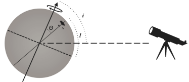
Figure 1: Illustration of a hotspot at latitude $l$ on the surface of a star viewed at inclination $i$ (inclination between the rotation axis and the observer’s line of sight). The magnetic obliquity is identified as the angle $\Theta$.

As many other emission lines associated with accretion onto a young star, the HeI$\lambda$5876 line is often composed of more than one component. Beristain et al. (2001) studied a number of He I profiles in CTTSs and found that they often present a narrow component (NC) and a broad component (BC). It is the NC that is believed to arise in the post-shock region, near the stellar surface, while the BC seems to have a composite origin. Beristain et al. (2001) found that the BC is sometimes observed blueshifted, in which case they attribute it to emission from a hot wind. When it is redshifted, they attribute it to emission from the accretion columns. Since all of these phenomena tend to be dynamic, these components will generally all be variable in their own way. Therefore in order to study one phenomenon or the other, it is important to either study systems that are dominated by one component, or to properly disentangle them. In the present study we attempt to do both.

We propose here to estimate the magnetic obliquity of a sample of well-known accreting T Tauri stars in the Taurus-Auriga star forming region, using the radial velocity variations of the NC of the HeI$\lambda$5876 line. We describe our observations in Sect. 2 and the method we use to derive hotspot latitudes in Sect. 3. The results obtained for each object are detailed in Sect. 4. We discuss our main findings in Sect. 5 and summarize our conclusions in Sect. 6.

2 Observations

Table 1: Journal of Observations

Name	Dates	Nspec	S/N600nm	<$V_{rad}$>	$\sigma V_{rad}$	<$v\sin i$>	$\sigma v\sin i$	Classification	Spectral type	Mass
	(Nov.2011)			(km s-1)	(km s-1)	(km s-1)	(km s-1)			M⊙
DE Tau	21-28	13	26-33	14.66	0.61	8.38	0.54	CTTS	M2.3	0.38
DF Tau	20-28	15	16-35	17.42	2.42	7.27	1.77	CTTS	M2.7	0.32
DK Tau	21-28	15	21-35	15.82	2.38	12.69	2.18	CTTS	K8.5	0.68
DN Tau	20-28	16	23-37	16.79	0.44	8.69	0.30	CTTS	M0.3	0.55
GI Tau	21-28	11	24-34	17.06	0.53	9.23	0.51	CTTS	M0.4	0.58
GK Tau	21-28	15	24-35	16.56	1.94	19.06	3.36	CTTS	K6.5	0.76
GM Aur	20-27	14	21-36	14.95	0.98	12.59	1.02	CTTS	K6.0	0.88
IP Tau	21-28	10	19-33	15.98	1.73	9.73	0.86	CTTS	M0.6	0.59
IW Tau	20-28	15	27-46	16.03	0.30	8.53	0.30	WTTS	M0.9	0.49
T Tau	18-28	26	14-39	19.47	1.28	23.54	1.61	CTTS	K0	1.99
V826 Tau	18-22	5	21-47	12.95	14.42	5.59	2.83	WTTS	K7	0.74
V836 Tau	23-28	7	30-33	17.73	0.86	10.51	0.77	CTTS	M0.8	0.58

Notes: Spectral types and masses are from Herczeg & Hillenbrand (2014).

Observations were carried out from November 18 to 28, 2011, at Observatoire de Haute-Provence using the SOPHIE spectrograph (Perruchot et al., 2008) in High-Efficiency mode, which delivers a spectral resolution of $R\sim 40,000$. The sample consists of ten accreting T Tauri stars (CTTS) and a control sample of two non-accreting T Tauri stars (WTTS). A total of 162 spectra were obtained, comprising between 10 and 16 spectra for each source in the CTTS sample over eight nights (Nov. 21-28), with up to 26 spectra for T Tauri itself over 11 nights (Nov. 18-28), and 5-7 spectra for each of the two WTTS of the control sample over the same time frame. The Journal of Observations is given in Table 1. Depending on the source brightness, exposure times varied between 137 s (e.g., T Tau) and 4410 s (e.g., IP Tau). The resulting signal-to-noise ratio (S/N) at the continuum level around 600 nm ranges from 15 to 50, with 2/3 of the spectra having S/N$\geq$30.

The raw spectra were fully reduced at the telescope by the SOPHIE real-time pipeline (Bouchy et al., 2009). The data products include a re-sampled 1D spectrum with a constant wavelength step of 0.01 Å, corrected for barycentric radial velocity, an order-by-order estimate of the signal-to-noise ratio, and a measurement of the source radial velocity, $V_{rad}$, and projected rotational velocity, $v\sin i$. These were derived from a cross-correlation analysis between the spectrum and a spectral mask template, either a G2 or a K5 mask, depending on the source’s spectral type (e.g., Melo et al., 2001; Boisse et al., 2010). We list the values of these parameters in Table 1 and use them for the subsequent analysis. The error quoted on $V_{rad}$ and $v\sin i$ in Table 1 is the standard deviation of individual measurements. While the latter are usually accurate to within a fraction of a km s^-1, the photospheric line profile variability induced by surface spots and/or the accretion flow in young stars yields much larger uncertainties (e.g., Petrov et al., 2001). The cross-correlation profiles themselves are presented in the online material and their night-to-night variations discussed there.

Figure 2: The HeI$\lambda 5876$ line profiles of CTTS and WTTS observed in this study. Thin lines: individual line profiles. Thick black line: averaged He I line profile. For clarity, the profiles shown here have been boxcar smoothed over 15 pixels (0.15 Å).

All 1D spectra were normalized to a continuum level of unity in the spectral region of interest. This was done using an IDL routine that identifies the continuum of a portion of the spectrum and fits a polynomial (of fourth or fifth order, depending on the curvature of the spectrum) through it. The continuum is identified by first manually excluding regions with emission lines, then taking only the points with the 20% highest intensities in order to exclude absorption lines. The portion of the spectrum of interest is then divided by the function that fits the continuum, resulting in normalized spectra. The final normalized spectra are shown in the online supplementary material.

3 Spectral analysis: line profile Doppler shifts

We aim at measuring Doppler shifts on the HeI$\lambda 5876$ line as a function of rotational phase. The line profiles for our stellar sample are shown in Fig. 2. With the exception of V826 Tau, which has very weak He I emission that is only measurable in one observation, we see that the He I line is observed in emission on every night for every star in this sample. This may seem unexpected if this emission comes from a rotationally modulated hotspot, since we would expect the spot to be behind the star in at least some epochs. We do note, however, that several stars show a significant decrease in the He I line flux during certain epochs (this can be seen in Fig. 2). This could occur if the spot passes behind the star, but a small portion of it always remains visible, because of the system inclination and spot latitude. Studies of ZDI have shown that it is common for the hotspot to be found at high latitudes (e.g. Donati et al., 2008, 2010b, 2011a), which would indeed lead them to be observable during most of the rotational cycle.

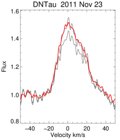
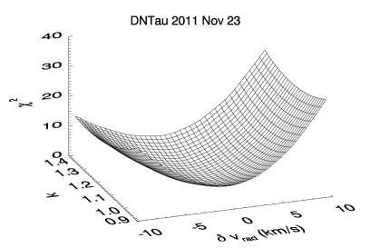
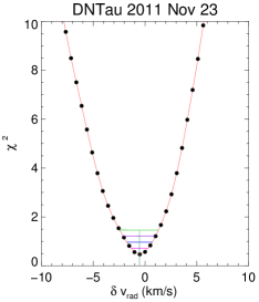
Figure 3: Left panel: the He I line profile of DN Tau obtained on Nov. 23 (lower solid line) is wavelength shifted and intensity scaled (upper solid line) to fit the average He I profile (thick red solid line) of the spectral series. The best fit (lowest $\chi_{\nu}^{2}$) solution is shown here. Middle panel: The $\chi_{\nu}^{2}(k,\delta V_{rad})$ surface is a shallow valley with a much steeper curvature along the radial velocity shift ($\delta V_{rad}$) axis than along the intensity scaling axis ($k$). Right panel: A cut in the $\chi_{\nu}^{2}$ surface around the $\chi_{\nu}^{2}$ minimum along the $\delta V_{rad}$ axis is taken (black dots) and linearly re-sampled (red curve). A sub-pixel estimate of the velocity shift is obtained by computing the centroid of the core of the $\chi_{\nu}^{2}(\delta V_{rad})$ curve over 4 velocity ranges (coloured horizontal lines). The adopted velocity shift $\delta V_{rad}$ is computed as the mean of the 4 centroid estimates and the 1$\sigma$ limits on $\delta V_{rad}$ are derived at the corresponding $\chi^{2}_{1\sigma}=\chi^{2}_{min}+1$ value.

To measure the Doppler shift on each night, we first define a reference profile for each star, to which the profiles from each night are compared. We initially used as reference the line profile with the best S/N and performed the analysis described in this section to find the shifts between this and all other profiles obtained from the spectral series of that star. We then shifted each of these $N$ line profiles in velocity space so they would coincide as closely as possible with each other. We take the mean of these $N$ shifted profiles as the final reference. This is done so as to obtain a mean line profile without artificially broadening it by combining lines at slightly different radial velocities.

The line profile of each night is intensity scaled by a factor $k$ and Doppler shifted by an amount of $\delta\lambda$ in order to fit the reference profile (see Fig. 3). For each spectrum in the series, the best fit parameters, $k$ and $\delta\lambda$, are obtained by minimizing the quantity

$$\chi_{\nu}^{2}(k,\delta\lambda)=\sum_{i=1}^{n}w_{i}^{2}\frac{\left[k\cdot(I(\lambda_{i}+\delta\lambda)-1)-(\left<I(\lambda_{i})\right>-1)\right]^{2}}{(n-2)\sigma_{cont}^{2}},$$ (2)

where $n$ is the number of spectral pixels over the line profile, $w_{i}$ is the weight applied to each pixel, $k$ is a scaling factor that accounts for line intensity variations, $I(\lambda)$ the intensity of the individual profile, $\delta\lambda$ the Doppler shift, $\left<I(\lambda)\right>$ is the intensity of the reference profile, and $\sigma_{cont}$ is the rms noise of the spectrum at the continuum level next to the line. The summation runs over $\pm$2.5$\sigma$ from the line centre, where $\sigma$ is the standard deviation of a Gaussian fit to the average line profile.

A first guess to the scaling factor $k$ is provided by the ratio between the maximum intensity of the average and individual profiles. The scaling parameter is allowed to vary within 20% of their ratio in 30 incremental steps. Doppler shifts are explored over a range of $\pm$25 km s^-1, with a spectral pixel step of 0.01 Å, corresponding to $\sim$0.5 km s^-1. Weights, $w_{i}$, which are chosen to scale as a Gaussian function (determined via a Gaussian fit to the reference profile), are applied to the $\chi_{\nu}^{2}$ calculation of each profile, in order to effectively increase the importance of the line core relative to the wings during the fitting procedure. For each profile, maps of $\chi_{\nu}^{2}(k,\delta\lambda)$ are computed and the location of the deepest $\chi_{\nu}^{2}$ minimum is found. As the two model parameters are independent, the $\chi_{\nu}^{2}$ surface is a shallow valley, whose main axis lies along the $k$ dimension (see Fig. 3). We therefore proceed to obtain a sub-pixel estimate of the location of the $\chi_{\nu}^{2}$ minimum in the $(k,\delta\lambda)$ grid by extracting a cut of the $\chi_{\nu}^{2}$ surface perpendicular to the $k$ direction around the deepest minimum. The $\chi_{\nu}^{2}(\delta\lambda)$ curve thus obtained is re-sampled and a sub-pixel estimate of its centroid is derived to provide the final estimate on $\delta V_{rad}$, the Doppler shift between the individual and average He I line profiles (see Fig. 3). Finally, the 1$\sigma$ uncertainty on $\delta V_{rad}$ is derived along the $\chi_{\nu}^{2}(\delta\lambda)$ curve at the location where $\chi_{\nu}^{2}=\chi_{\nu,min}^{2}+1$ (Press et al., 1992). The whole procedure is illustrated in Fig. 3.

Care must be taken when using this procedure on the stars whose HeI$\lambda 5876$ line profiles show more than one component, which is the case for DE Tau, DF Tau, GM Aur and T Tau. These components are believed to have different origins and therefore should present different variabilities (Beristain et al., 2001). The magnetic obliquity is related to the variability of the narrow component (NC), which is believed to arise in accretion shocks close to the stellar surface. Therefore, in the cases where a broad component (BC) is also present, we first fit the individual profiles from each night with two Gaussians in order to identify the two components, then analyse only the variability of the narrowest of the two components. However, the profiles that present only one component show that the NC is not symmetric. Thus, taking the centroid of the narrowest Gaussian component may introduce small uncertainties to the radial velocity measurements. On the other hand, a visual inspection of the profiles studied by Beristain et al. (2001, see their Fig. 1a) shows that the BC often seems to be nearly symmetric and reasonably well reproduced by a Gaussian (this is not always the case, particularly for the strongest accretors, such as AS 353A, DG Tau, DR Tau and RW Aur, all of which show more complex profiles, but it seems to be the case for the four stars in our sample). Therefore, to isolate the NC, we subtract the broadest Gaussian component from the composite profiles to remove the contribution of the BC. We then perform the cross-correlation analysis described above on the residual profile, which should contain only the contribution from the NC. We note that, in our sample, a typical NC has a full width at half maximum (FWHM) of $\sim 35$ km s^-1, while a typical BC has FWHM $\sim 120$ km s^-1. Figure 4 shows an example of the Gaussian fit and residual profile of each of these stars.

We find that the radial velocity measurements of the residual profiles agree, within the uncertainties, with the centroid velocities of the narrowest component of the Gaussian decomposition. In the case of DE Tau, DF Tau and GM Aur, the results also agree with the ones obtained from the cross-correlation of the full HeI$\lambda 5876$ line profile (without subtracting the BC), though the error bars are larger when the BC is not removed. We can see in Fig. 4 that the BC mostly affects the wings of these profiles, while the centre of the line is dominated by the NC. Therefore, by allowing the computation of $\chi_{\nu}^{2}$ to run over $\pm 2.5\sigma$ of a Gaussian approximation to the centre of the line, the broad wings are ignored and as a result the BC does not strongly interfere with the analysis. For the star T Tau, however, the HeI$\lambda 5876$ line profile is clearly dominated by the BC. In this case, the cross-correlation analysis of the full profile yields very different results than when the contribution of the BC is removed. For this star, removing the contribution of the BC is essential to properly identify the latitude of the accretion shocks. The Gaussian decomposition of all observations of the star T Tau can be seen in the online material (except for two observations, which have been excluded due to low S/N).

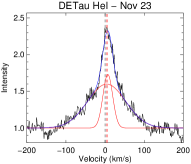
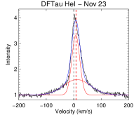
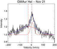
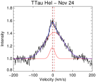
Figure 4: Left panels: Examples of the Gaussian decomposition performed on the HeI$\lambda 5876$ line profiles that presented two components. Right panels: residual profiles obtained after subtracting the broad component from the observed spectrum.

4 Results

4.1 Variability of the He I line

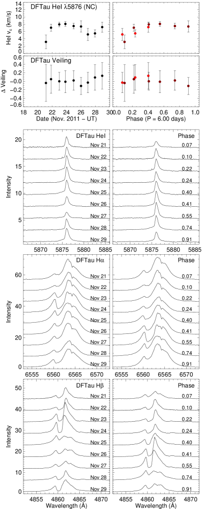
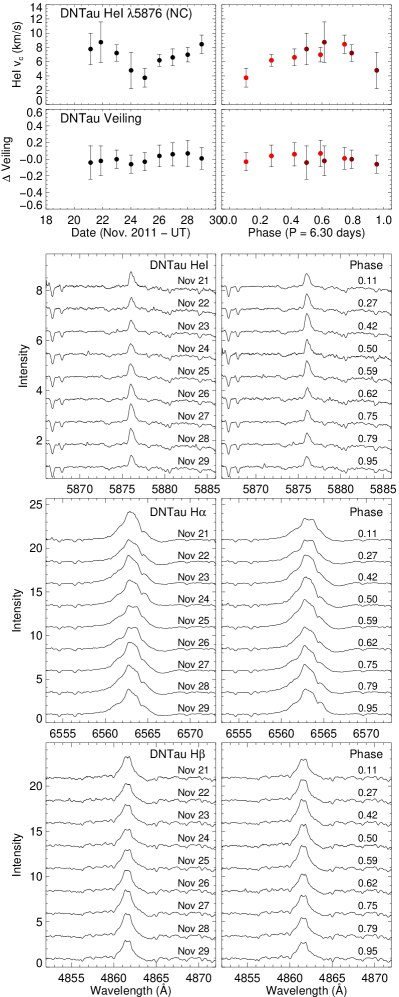
Figure 9: Variability of the radial velocity of the HeI$\lambda 5876$ narrow component, veiling, the HeI$\lambda 5876$ profile, the H$\alpha$ profile and the H$\beta$ profile for the rest of the stars in our sample, shown in full (left panels) and folded in phase using the period believed to be the stellar rotation period (right panels). Different colors represent different rotation cycles. The initial dates for the phase calculation are shifted by the amount necessary for the hotspot to be in full view around phase $\phi=0.5$. Thus, in a few cases, the phase plots show three colours even though the star was only observed over two rotation periods.

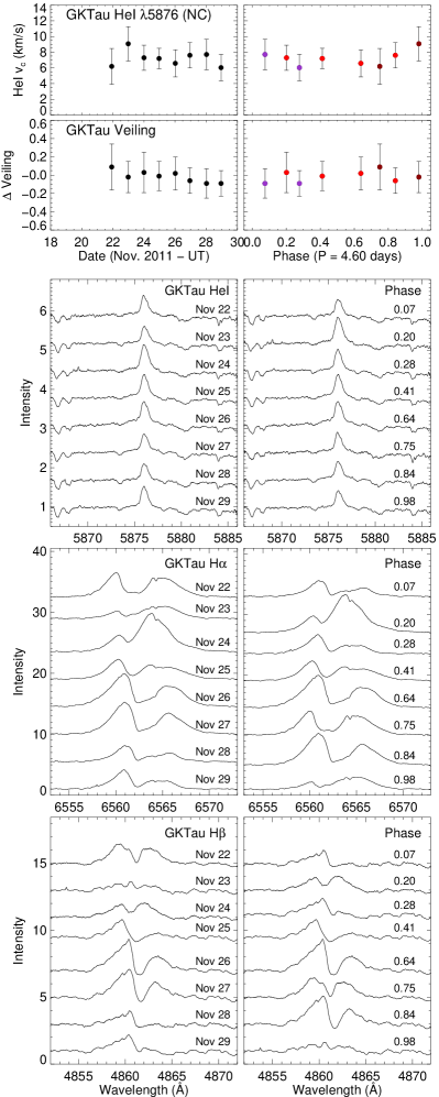
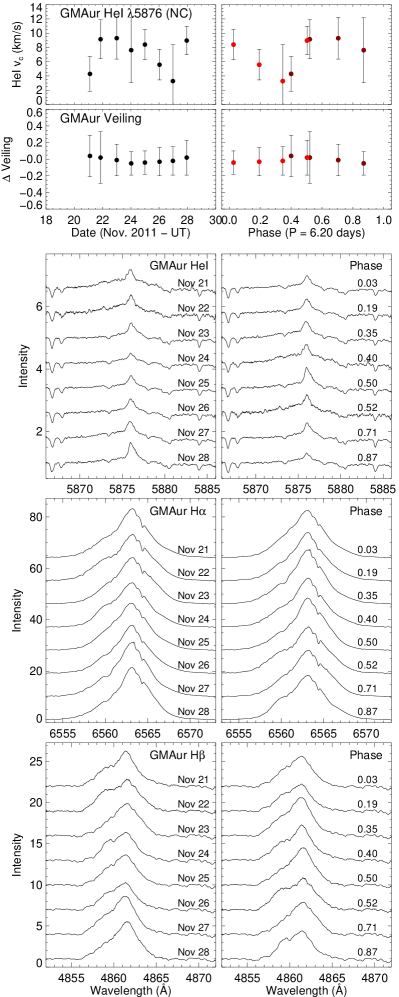
Figure 9: Continued.

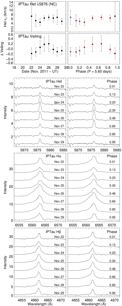
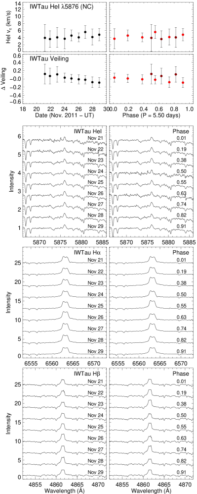
Figure 9: Continued.

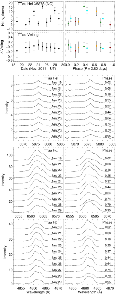
Figure 9: Continued.

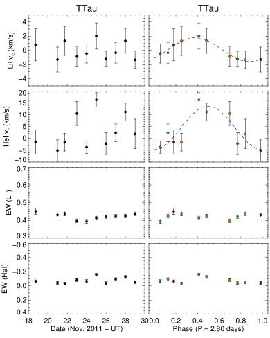
Figure 10: Plots showing the variability of the radial velocity of the LiI$\lambda 6708$ line, the radial velocity of the HeI$\lambda 5876$ line, the equivalent width of the LiI$\lambda 6708$ line and the equivalent width of the HeI$\lambda 5876$ line. Right panels show the same plots as the left panels, but folded in phase with the stellar rotation period. Different colors represent different rotation cycles.

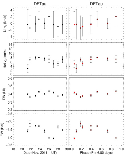
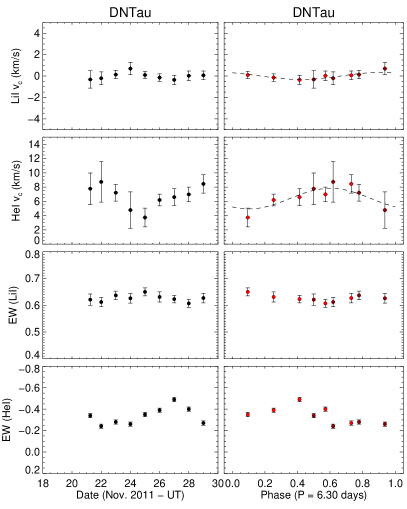
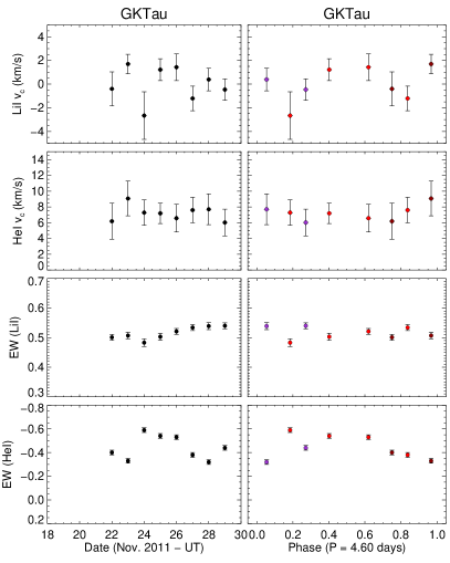
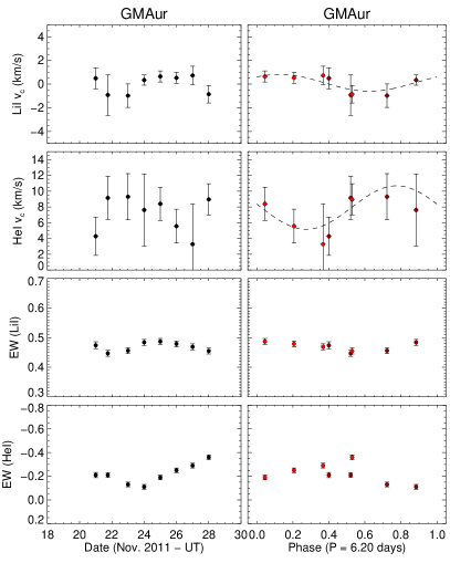
Figure 10: Continued.

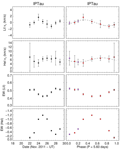
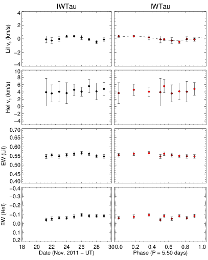
Figure 10: Continued.

We present in this section the results obtained for the radial velocity variations of the HeI$\lambda 5876$ line profile of a sample of accreting T Tauri stars. The hotspot latitudes derived from the radial velocity variations of each star and Eq. 1 are shown in Table 2. The variability of the narrow component of the He I line and the veiling variability (with respect to the mean spectrum) for each star in our sample can be verified in Figs. 8 and 9 of the Appendix. Veiling was measured in a region near the He I line where several photospheric absorption lines are present. The spectrum of each night was compared with the mean spectrum of the same star, in order to find the amount of excess continuum emission that minimized $\chi^{2}$. The uncertainties (derived at the corresponding $\chi^{2}_{1\sigma}=\chi^{2}_{min}+1$ value) are large, but some of the trends seen in veiling appear to be confirmed by the variability of the equivalent width (EW) of the LiI$\lambda$6708 line (Fig. 10). The EW of this line (or any deep photospheric absorption line) gives an indirect measurement of veiling, since the excess emission causes the photospheric absorption lines to appear shallower in the normalized spectrum, reducing their EW.

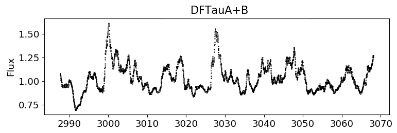
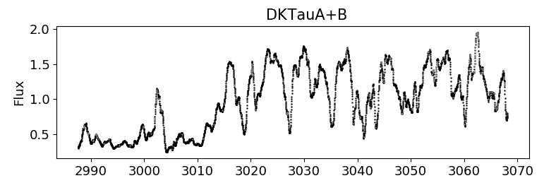
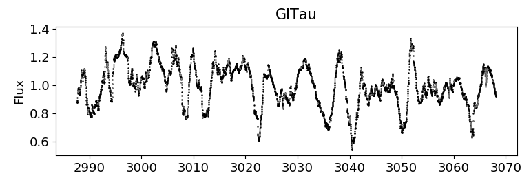
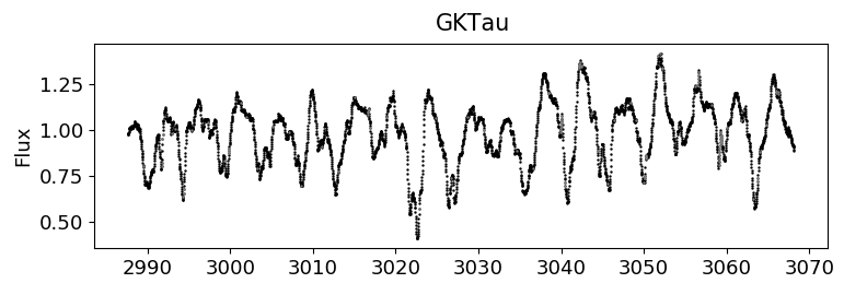
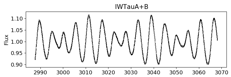
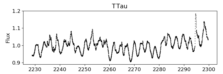
Figure 11: Light curves of the stars in our sample that were observed by K2.

Our analysis also partly rests upon the pattern of spectral variability observed in other lines, such as H$\alpha$ and H$\beta$ (whose profiles are also shown in Figs. 8 and 9 and in more detail in the online material), as well as LiI$\lambda$6708 (whose radial velocity curves and equivalent width variability can be seen in Fig. 10, alongside the variability of $V_{rad}$ and EW of the He I line), and K2 light curves (shown in Fig. 11). The Li I line profiles can be seen in the online material. Due to the specific behaviour of line profile variability in each object, we discuss each sample source in turn.

Table 2: Hotspot latitudes and magnetic obliquities

Star	$\Delta V_{rad}$(HeI)	$v\sin i$	$\cos l$	$l$	$\Theta$
	(km s-1)	(km s-1)		(∘)	(∘)
DE Tau	1.8$\pm$3.2	8.4$\pm$0.5	0.11$\pm$0.19	84$\begin{subarray}{c}+6\\ -11\end{subarray}$	6$\begin{subarray}{c}+11\\ -6\end{subarray}$
DF Tau	3.7$\pm$2.2	7.3$\pm$1.8	0.25$\pm$0.16	75$\pm 10$	15$\pm 10$
DK Tau	7.8$\pm$2.8	12.7$\pm$2.2	0.31$\pm$0.12	72$\begin{subarray}{c}+7\\ -8\end{subarray}$	18$\begin{subarray}{c}+8\\ -7\end{subarray}$
DN Tau	3.8$\pm$3.0	8.7$\pm$0.3	0.22$\pm$0.17	77$\begin{subarray}{c}+10\\ -11\end{subarray}$	13$\begin{subarray}{c}+11\\ -10\end{subarray}$
GI Tau	3.8$\pm$2.8	9.2$\pm$0.5	0.21$\pm$0.15	78$\pm 9$	12$\pm 9$
GK Tau	3.0$\pm$4.6	19.1$\pm$3.4	0.08$\pm$0.12	85$\begin{subarray}{c}+5\\ -7\end{subarray}$	5$\begin{subarray}{c}+7\\ -5\end{subarray}$
GM Aur	5.9$\pm$6.6	12.6$\pm$1.0	0.23$\pm$0.26	77$\begin{subarray}{c}+13\\ -16\end{subarray}$	13$\begin{subarray}{c}+16\\ -13\end{subarray}$
IP Tau	2.2$\pm$3.9	9.7$\pm$0.9	0.11$\pm$0.20	83$\begin{subarray}{c}+7\\ -12\end{subarray}$	7$\begin{subarray}{c}+12\\ -7\end{subarray}$
IW Tau	1.9$\pm$4.1	8.5$\pm$0.3	0.11$\pm$0.24	84$\begin{subarray}{c}+6\\ -14\end{subarray}$	6$\begin{subarray}{c}+14\\ -6\end{subarray}$
T Tau	18.4$\pm$7.9	23.5$\pm$1.6	0.39$\pm$0.17	67$\begin{subarray}{c}+10\\ -11\end{subarray}$	23$\begin{subarray}{c}+11\\ -10\end{subarray}$
V836 Tau	3.7$\pm$4.3	10.5$\pm$0.8	0.17$\pm$0.21	80$\begin{subarray}{c}+10\\ -12\end{subarray}$	10$\begin{subarray}{c}+12\\ -10\end{subarray}$

4.1.1 DE Tau

This star’s spectrum presents veiling that is clearly variable in the time-scale of the observations. The veiling increases steadily to reach a maximum on Nov. 26, then drops again, consistent with the rotation period of 7.6 days taken from the literature (Bouvier et al., 1993). The intensity of the He I line reaches its maximum two days before the veiling maximum, on Nov. 24. The H$\alpha$ and H$\beta$ line profiles are more intense than average on both these nights, but show no clear trend with the 7.6 day period.

4.1.2 DF Tau

The intensity of the He I line profile, as well as its radial velocity variability, appear to be modulated on a time-scale of around 6 days, though the time-sampling of our observations is not enough to determine an accurate rotation period. This value is different from the photometric periods given in the literature, of 8.5 days (Bouvier et al., 1995) and 7.18 days (Artemenko et al., 2012). However, neither of these two periods are found in this star’s K2 light curve (N. Roggero private communication). The He I line shows the lowest intensities just before it is most blueshifted, which is consistent with an origin in a stellar spot modulated by rotation. The veiling variability has too small an amplitude to derive any conclusions from it. However, the H$\alpha$ and H$\beta$ line profiles also show a trend with the $\sim$6 day period, where a blueshifted absorption component appears at phase $\phi\sim 0.6$, just after the accretion shock has passed in front of our line of sight (the He I line profile is more redshifted than average). Since this component is associated with outflows intersecting our line of sight, this points to a spatial association between the accretion shocks and a wind. This could be a stellar wind or a non-axisymmetric disc wind that is launched close to the co-rotation radius, in order to show periodic behaviour on the same time-scale as the stellar rotation.

4.1.3 DK Tau

The intensity and radial velocity of the He I line, as well as the veiling, show a variability that is modulated on the time-scale of the observations (the variability of veiling is just within the error bars, but the trend is confirmed by the EW of the LiI line in Fig. 10). As the He I line passes in our line of sight, its radial velocity going from blueshifted to redshifted with an amplitude of $\sim 10$ km s^-1, the veiling and He I intensity increase to reach a maximum on Nov. 25 and Nov. 27, before decreasing again. However, something occurs on Nov. 26 which results in a less intense, more centred He I line, less veiling and much less intense H$\alpha$ and H$\beta$ line profiles. If not for this event, the behaviour of He I and veiling in this star would be consistent with the rotational modulation of a hotspot on the stellar surface with the reported period of 8.18 days (Percy et al., 2010; Artemenko et al., 2012). It is possible that on this date, circumstellar material passed in front of the line of sight, partially obscuring the hotspot and resulting in the less intense emission lines and veiling. Its K2 light curve appears to be dominated by flux dips (see Fig. 11), which is consistent with circumstellar material obscuring the star from time to time. The H$\beta$ line shows an inverse P Cygni profile on Nov. 24 and 25, just before this event. This type of profile, characterized by a redshifted absorption, occurs when the accretion funnel flows intersect our line of sight.

4.1.4 DN Tau

The intensity and radial velocity of the He I and Li I lines are modulated with a period that is consistent with the value of 6.32 days given in the literature for this star’s rotation period (Donati et al., 2013; Artemenko et al., 2012). The radial velocity variability of the Li I line appears to be mirrored with respect to the He I line (Fig. 10). This is consistent with rotational modulation of an accretion shock. While the He I emission originating in the hotspot will be more blueshifted as this spot comes into view and more redshifted as it recedes, photospheric absorption lines such as Li I appear more redshifted as a hot (or cold) spot comes into view and more blueshifted as it recedes, since the line is deformed due to the presence of spots on the stellar surface (see e.g. Gahm et al., 2013). The amplitude of the veiling variability is too small to draw any conclusions from it.

This star’s H$\alpha$ and H$\beta$ line profiles present a redshifted absorption component in some observations, which is clearest on Nov. 27, when the He I line is strongest and more centred, meaning that the accretion shock is in full view. As this redshifted absorption originates in accretion funnel flows crossing our line of sight, this points to a spatial association between the accretion shocks and funnel flows.

4.1.5 GI Tau

The intensity of the main emission line profiles (H$\alpha$, H$\beta$, He I) is modulated on the time-scale of the observations. The intensity of the residual line profiles steadily decreases from Nov. 22-23 to reach a minimum around Nov. 27, then increases again up to Nov. 29, a behaviour which is consistent with the modulation of the line flux by a bright spot rotating with a period of $\sim$7 or 8 days. This is in agreement with the past reported photometric period of 7.1 days (Percy et al., 2010; Artemenko et al., 2012). The veiling appears to decrease over a similar time period, however the variability amplitude is within the uncertainties and therefore cannot be confirmed.

4.1.6 GK Tau

The variability of the radial velocity of the He I line is consistent with a period of 4.6 days, found in the literature (Percy et al., 2010; Artemenko et al., 2012) and in this star’s K2 light curve (Rebull et al., 2020). There is no clear trend in veiling or in the H$\alpha$ and H$\beta$ line profiles with this period, even though the variability of the line profiles is very strong.

4.1.7 GM Aur

The intensity of the He I line is modulated on the time-scale of the observations, decreasing until Nov. 24, then increasing again. The variability of this line’s radial velocity is consistent with rotational modulation of a spot with the period of 6 days given in the literature (Percy et al., 2010; Artemenko et al., 2012). The veiling variability is too small to draw any conclusions from it. As with DN Tau, the radial velocity variability of the Li I line is mirrored with respect to the He I line, in support of rotational modulation of a hotspot. There is no clear trend in the H$\alpha$ and H$\beta$ line profiles with this period.

4.1.8 IP Tau

The intensity and radial velocity of the He I and Li I lines, as well as the veiling, all show a variability that is consistent with a period of 5.6 days. Veiling increases along with the intensity of He I, both reaching a maximum on Nov. 25, while the He I line profile went from more blueshifted than average on Nov. 23 and 24, to more redshifted on Nov. 25-28, and the Li I line went from more redshifted to more blueshifted in this same time. This behaviour is consistent with the veiling and He I line being modulated by a hotspot rotating at this period, which is different from the photometric period of 3.25 days found by Bouvier et al. (1993). The light curve from that study was therefore likely dominated by something other than rotational modulation from spots on the stellar surface.

The H$\alpha$ and H$\beta$ line profiles show a redshifted absorption component on one night (Nov. 29), corresponding to phase $\phi\sim 0.25$, when the He I line is more blueshifted and veiling is beginning to increase, meaning that the accretion shock is appearing in our line of sight. As was the case with DN Tau, this points to a spatial association between the accretion funnel flows and accretion shocks.

4.1.9 IW Tau

This star was one of the two WTTSs (non-accreting T Tauri stars) in our control sample. It shows a relatively narrow H$\alpha$ line profile, with a width at 10% of the maximum intensity of only 180 km s^-1, which is much lower than the threshold of 270 km s^-1 usually used to classify a T Tauri star as actively accreting (White & Basri, 2003). Therefore it would not be classified as a classical T Tauri star based on its H$\alpha$ line profile. However, this star does present a weak He I emission line with a redshift of 4.3 $\pm$ 0.8 km s^-1, which does not seem to be variable in our observations. Beristain et al. (2001) also observed weak HeI$\lambda 5876$ emission in the spectra of three non-accreting T Tauri stars, however they were all on average centred at the stellar rest velocity, which led to the conclusion that they could be the result of very active chromospheres. The He I emission we observe in IW Tau is redshifted at above 3$\sigma$, which means it must originate in material falling onto the star.

It is possible that this star is still undergoing accretion at a very reduced rate. In order to test this possibility, we estimated a mass accretion rate for this star from several emission lines in its spectra, following the relations given by Alcalá et al. (2017). We find an average value for the logarithmic mass accretion rate of $\log\dot{M}_{acc}=-9.5(\pm 0.3)~{}\mathrm{M}_{\odot}~{}\mathrm{yr}^{-1}$ (corresponding to $\dot{M}_{acc}=3\times 10^{-10}~{}\mathrm{M}_{\odot}~{}\mathrm{yr}^{-1}$), where the uncertainty in $\log\dot{M}_{acc}$ represents the standard deviation across the ten emission lines used to calculate accretion luminosity. It is worth noting that this likely represents an upper limit to this star’s mass accretion rate, since at these low levels of emission, these lines may be affected by chromospheric activity in a non-negligible way. At the same time, the strong agreement between the mass accretion rates derived from all these different lines (made clear by the relatively small dispersion in the values found) is a good indication of the reliability of this result. This star does not seem to be surrounded by a circumstellar disk (besides possibly a thin debris-disk, typical of WTTSs in general; Beckwith et al., 1990; Wolk & Walter, 1996; Furlan et al., 2005).

This star’s Li I line is modulated on a 5.5 day time-scale, which could be caused by the rotational modulation of cold spots on the stellar surface, or by a binary companion (since this star has been reported to be a binary system by Richichi et al., 1994). This star’s K2 light curve clearly shows a spot-like behaviour, with two distinct periods, one of which agrees with this period found in the Li I line (see Fig. 11 and Rebull et al., 2020). It is likely that one of these periods represents the star’s rotation while the other may be due to a companion.

4.1.10 T Tau

This is a multiple system, consisting of three stars (known as T Tau N, Sa and Sb; Koresko, 2000; Köhler et al., 2000), although the secondary component T Tau S(a+b) is not detectable in optical wavelengths, likely because of strong extinction from circumstellar or circumbinary material (Duchêne et al., 2005). Thus the spectra presented here are entirely dominated by the brightest component, T Tau N.

The radial velocity of this star’s He I NC is very well modulated with a period of 2.7$\pm$0.4 days, while the radial velocity of the Li I line gives a similar period of 2.86 days. These periods coincide well with the photometric period of 2.81 days measured by Artemenko et al. (2012) and in its K2 light curve (Rebull et al., 2020). The top two panels of Fig. 5 show the Li I line and the NC of the He I line folded in phase with this period of $P=2.8$ days. The variability amplitude of the veiling is small, and there are no clear trends in the H$\alpha$ or H$\beta$ lines with the stellar rotation period. We can see that the modulus of the equivalent width of the He I line’s NC is largest when it is most redshifted (on Nov. 25 and Nov. 28), which may be due to a favorable viewing geometry. We have found that the magnetic obliquity of this star is $\theta=(23\pm 10)^{\circ}$, which agrees, within the uncertainties, with its system inclination of $i=(28\pm 1)^{\circ}$ (Manara et al., 2019). This means that when the accretion shock passes in front of us, we observe the flow of matter onto the star projected almost directly in our line of sight.

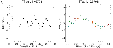
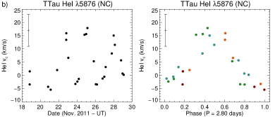
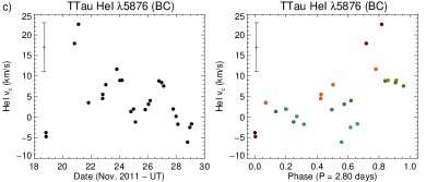
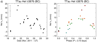
Figure 5: Radial velocity variability of a) the Li I line; b) the narrow component of the He I line; c) and d) the broad component of the He I line, for the star T Tau. The plots are shown in full in the left panels and in phase in the right panels, using the period of $P=2.8$ days (panels a, b and c) and $P=3.1$ days (panel d). Different colors represent different rotation cycles. The median error bar on the radial velocity is shown on the top left corner of each plot. In these plots, we do not show the average measurement in each night, but rather include all observations.

Another interesting aspect of this star’s He I line profile is that its BC also shows periodic radial velocity variability, but with a slightly longer period of 3.1$\pm$0.3 days. The bottom two panels of Fig. 5 show the radial velocity variability of this component folded in phase with the period of the NC ($P=2.8$ days) and with the longer period of $P=3.1$ days. It is clear that this component folds much better in phase with the longer period. In order to confirm whether these two slightly different periods are real and not an artefact of the Gaussian decomposition, we performed a 2-dimensional periodogram analysis on the full line (Fig. 6). From this figure it appears that the dominant period is the 3.1 day period of the BC, which is clear on the wings of the profile (especially the redshifted wing, between $\sim$40km s^-1 and 100km s^-1), where the BC dominates. However, near the centre of the line (around 5 - 10km s^-1, where the NC appears), the periodogram seems to split and shows a small peak at 2.7 days. If the full line originated in the hotspot, then this apparent quasi-periodicity could occur, for instance, if the hotspot were to move on the stellar surface, or to split into more than one spot. However, because the wings of the profile come from the BC, which is believed to have a different origin than the NC, it seems more likely that the two components of the He I line indeed have two slightly different periods. Since the period from the NC agrees well with the rotation period of 2.8 days found from photometry in the literature and also from the Li I line in this study, this likely represents the stellar rotation, while the slightly larger period of 3.1 days from the BC should be caused by a different phenomenon.

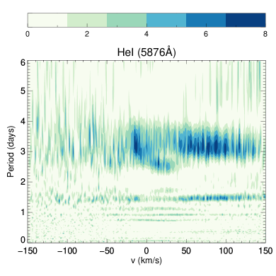
Figure 6: 2-dimensional periodogram of the He I line of T Tau. The abscissa shows the velocity bins (centred at stellar rest velocity) for which periodograms were measured, the ordinate shows the range of periods spanned, and the colour gradient represents the periodograms’ intensities.

According to Beristain et al. (2001), the broad component of the HeI$\lambda 5876$ line may come from a hot wind or from the accretion funnel flows. Since in T Tau this component is redshifted on average, it must be coming mostly from the accretion funnel flows at polar angles less than 54.7^∘ (see Fig. 9 of Beristain et al., 2001). If this is indeed the case, then a slightly larger period measured from this component when compared to the stellar rotation period may be an indication that there is differential rotation throughout the accretion funnel flow. This could be expected if a star’s magnetosphere were to truncate the inner disc at a radius larger than the co-rotation radius, resulting in the part of the accretion funnel flow that connects to the inner disc rotating more slowly than the stellar surface. The star would then accrete via the propeller regime, though this could be a temporary situation, not necessarily reflecting the steady state of the system. Its K2 light curve, for instance (which was observed in 2015 - four years after the spectroscopic observations in this paper), is periodic, which seems to indicate that this star was in a stable accretion regime at the time of the K2 observations (see Fig. 11).

We cannot, however, conclude with certainty that there is differential rotation in the accretion columns of T Tau, since the two periods found in fact agree within their error bars. A more in-depth study, with more accurate periods, would be necessary to confirm this hypothesis. Additionally, current radiative transfer models are incapable of reproducing the main characteristics of the broad component of the HeI$\lambda 5876$ line with standard accretion models (see, e.g. Kurosawa et al., 2011), so we cannot say for certain what is the origin of this broad emission.

4.1.11 V836 Tau

This star shows some variability in the radial velocity of its He I line, but no clear period can be distinguished in the 6-day observation, which is shorter than the period of 7.0 days given in the literature (Rydgren et al., 1984). The He I line intensity and veiling show little variability and no clear trend is seen in the H$\alpha$ or H$\beta$ line profiles.

4.2 Velocity of the flow of matter traced by He I

We estimate the velocity ($V_{flow}$) of the accretion flow that is traced by the narrow component of the HeI$\lambda 5876$ line for each star in our sample, by taking the median He I radial velocity of each star and de-projecting it from the line of sight. Therefore, $V_{flow}=~{}V_{rad,med}/\cos\alpha$, where $\alpha$ is the angle between the line of sight and the direction of the flow of matter onto the star. This angle is related to the system inclination ($i$ - given in Table 3) and the latitude of the accretion shock ($l$ - given in Table 2) through the relation $\alpha=|i-l|$ (see Fig. 1). Table 3 shows the derived flow velocities $V_{flow}$, as well as the mean ($<V_{rad}>$), median ($V_{rad,med}$) and standard deviation ($\sigma$) of the He I radial velocities measured in each star (with regard to the star’s rest velocity), the mean error in $V_{rad}$ measurements for each star, and the system inclinations $i$.

Table 3: Average radial velocities of the HeI$\lambda 5876$ line and resulting flow velocities

Star	$<V_{rad}>$	$V_{rad,med}$	$<errV_{rad}>$	$\sigma V_{rad}$	Inclination	Ref	$V_{flow}$
	(km s-1)	(km s-1)	(km s-1)	(km s-1)	(∘)		(km s-1)
DE Tau	5.84	5.96	1.19	0.81	$70\pm 7$	P14	14$\begin{subarray}{c}+38\\ -7\end{subarray}$
DF Tau	6.54	6.69	1.01	1.61	$19\pm 8$	*	6.7$\begin{subarray}{c}+1.6\\ -1.0\end{subarray}$
DK Tau	9.36	9.54	1.86	3.96	$13\pm 3$	M19	9.6$\begin{subarray}{c}+2.3\\ -1.9\end{subarray}$
DN Tau	6.68	7.36	0.99	1.40	$35\pm 1$	L18	7.9$\begin{subarray}{c}+2.1\\ -1.5\end{subarray}$
GI Tau	6.72	6.32	1.25	1.65	$29\pm 9$	*	7.9$\begin{subarray}{c}+9.4\\ -2.8\end{subarray}$
GK Tau	7.21	7.40	1.95	1.18	$71\pm 5$	S17	18$\begin{subarray}{c}+27\\ -9\end{subarray}$
GM Aur	7.10	7.90	2.72	2.56	$55\pm 1$	T17	10.6$\begin{subarray}{c}+10.0\\ -4.9\end{subarray}$
IP Tau	5.99	6.14	1.08	0.87	$45\pm 1$	L18	7.8$\begin{subarray}{c}+3.7\\ -2.2\end{subarray}$
IW Tau	4.33	4.14	0.77	0.77	$33\pm 9$	*	4.6$\begin{subarray}{c}+3.0\\ -1.3\end{subarray}$
T Tau	4.20	2.00	5.19	7.55	$28\pm 1$	M19	2.0$\begin{subarray}{c}+5.5\\ -5.2\end{subarray}$
V836 Tau	6.01	6.22	1.30	1.12	$61\pm 10$	T17	10$\begin{subarray}{c}+16\\ -4\end{subarray}$

Notes: The second and third columns show the mean and median radial velocity of He I for each star, column 4 shows the mean error on the radial velocity measurements, columns 5 and 6 give the inclination to the system and its reference, and the final column shows the flow velocity derived for each star. References for inclinations are Piétu et al. (2014) (P14), Manara et al. (2019) (M19), Long et al. (2018) (L18), Simon et al. (2017) (S17), Tripathi et al. (2017) (T17), and those marked with an asterisk have no direct measurement of the disc in the literature, so inclinations were estimated using the relation $v\sin i=(2\pi R_{*}/P_{rot})\sin i$, where $P_{rot}$ and $v\sin i$ are given in this paper, and $R_{*}$ was taken from Herczeg & Hillenbrand (2014).

Average $<V_{rad}>$	$\sigma<V_{rad}>$	Average $V_{flow}$	$\sigma V_{flow}$
(km s-1)	(km s-1)	(km s-1)	(km s-1)
6.4	1.4	9.0	4.3

5 Discussion

5.1 Comparison with other observational studies

As can be seen in Table 2, the magnetic obliquities we find for the stars in our sample are between 5^∘ and 23^∘, with most (80%) below 15^∘. Therefore in our sample the magnetic fields seem to be generally well aligned with the stellar rotation axis, which is somewhat in disagreement with what has been found from direct magnetic field measurements in T Tauri stars, many of which have a misalignment larger than 20^∘ (see Table 5 and, e.g., Johnstone et al., 2014). It is possible that our sample may be influenced by a selection bias. The stars in this sample were selected based mainly on two criteria: having shown periodic photometric behaviour in a previous study and presenting a HeI$\lambda 5876$ line profile in emission that is dominated by the NC. The only exception to the latter criterion is T Tau, which was observed mainly because of its brightness and is the only star in our sample for which the He I line is dominated by the broad component. It is also the star that shows the largest magnetic obliquity in this study, of 23^∘. It is possible that there may be a connection between the processes that originate the BC of the HeI$\lambda 5876$ line and large magnetic obliquities. This would lead to an observational bias in our sample, where by excluding stars that present very broad HeI$\lambda 5876$ emission, we exclude the stars with large magnetic obliquities. In order to confirm this hypothesis, we would need to study a much larger sample of CTTSs with more diverse He I line profiles.

The other selection bias that our sample could possibly be subject to is with periodicity, since the stars in our sample all have a measured period in the literature. However, it is difficult to find an explanation in which this leads to a bias towards magnetic obliquities smaller than $\sim 15^{\circ}$, since MHD models of Kurosawa & Romanova (2013) and Blinova et al. (2016) predict that larger magnetic obliquities should lead to stars accreting more often in a stable accretion regime, which is believed to produce periodic signatures in a star’s photometry. Therefore, based on these models, choosing a sample of stars with known periodicity should not lead us to exclude stars with large magnetic obliquities.

While studying the spectroscopic variability of the very active star EX Lupi, Sicilia-Aguilar et al. (2015) found a periodic signature in the radial velocity variation of different He I lines (at $\lambda=4713$Å, 5876Å, and 6678Å), as well as the HeII$\lambda 4686$ line, which were consistent with the rotational modulation of a hotspot on the stellar surface. They found, however, that the amplitudes of the radial velocity variations differ for the different lines, with lines with higher excitation potentials having larger amplitudes and a clearer modulation. In general, lines with different excitation potentials may originate in regions with different temperatures, which could be at different latitudes, longitudes (a spot may have the highest temperature at its core and be surrounded by regions of lower temperature), or height above the stellar surface (there may be a temperature structure along the accretion column, above the stellar surface, as has been detected by Dupree et al., 2012; Sicilia-Aguilar et al., 2017). This could explain the different amplitudes found by Sicilia-Aguilar et al. (2015) for the different lines.

If there is a difference in the temperature structure on the stellar surface along latitude, then this may help to explain our apparently low magnetic obliquities. By choosing the HeI$\lambda 5876$ line, which has a lower excitation potential than HeI$\lambda 4713$ and HeII$\lambda 4686$, we may be tracing a region that is at a slightly higher latitude than the central part of the accretion shock, which may be nearer to the magnetic pole. If true, this effect would probably bias the estimates of magnetic obliquity using this line to lower values, which may explain not only our sample, but also the fact that the three other stars from the literature whose obliquities were derived using the same method as the one described in our paper also present such low values of $\Theta$ (EX Lup, RU Lup and DR Tau, see Table 5 and Sicilia-Aguilar et al., 2015; Gahm et al., 2013; Petrov et al., 2011). However, this does not seem to be the case. Petrov et al. (2001) found the same amplitude (within error bars) for the radial velocity variability of He I and He II lines for the star RW Aur. Also, several studies of spectropolarimetry have found misalignements between the main component of the magnetic field and the stellar rotation axis that are consistent with the HeI$\lambda 5876$ variability amplitudes found in the same observations (e.g. BP Tau, AA Tau, LkCa15, and CI Tau; Donati et al., 2008, 2010b; Alencar et al., 2018; Donati et al., 2020).

We can also verify how the variability of photospheric lines compares with that of the He I lines. Crockett et al. (2012) studied the radial velocity variability of photospheric lines in optical and near-infrared spectra of several CTTSs, in order to study the effect of stellar spots on these lines. Their sample included four of the same stars as our sample. The amplitudes they found for the radial velocity variability of photospheric lines in optical wavelengths agree, within the uncertainties, with our amplitudes for the HeI$\lambda$5876 line, though the values for the photospheric lines are systematically lower, as expected for large cool spots.

5.2 Photometric variability

Blinova et al. (2016) predict that the location of the magnetospheric radius $R_{m}$ (the disc’s truncation radius) with respect to the disc’s co-rotation radius $R_{co}$ has a strong influence on the accretion regime, stronger than the magnetic obliquity ($\Theta$). None the less, for stars with magnetospheres of similar size, they predict that an increase of the magnetic obliquity leads to a decrease of the amplitude of the light curve oscillations that are associated with instabilities and an increase of the amplitude of the variability associated with the rotation of the star. According to Blinova et al. (2016), for small values of $\Theta$ ($\lesssim 5^{\circ}$ for $R_{co}\sim 1-1.4R_{m}$, or up to $\sim 10^{\circ}$ for smaller magnetospheres), the main source of variability should be unstable ordered hotspots and the light curve should be very irregular, though the stellar rotation period may still be found in the light curve’s Fourier spectrum. For slightly larger values of $\Theta$ ($\sim 15^{\circ}$), the stellar rotation period should become more evident, but many short-scale oscillations from instabilities could still be seen in the light curve. When $\Theta$ is around $\sim 20^{\circ}-30^{\circ}$, the oscillations from instabilities would have smaller amplitudes, leading to more regular light curves, but with the stellar rotation period becoming slightly less well defined in the Fourier spectrum.

Among the 11 stars in our sample with He I in emission, 6 were observed recently by the K2 mission (their light curves are shown in Fig. 11 and a more detailed analysis is explored in Rebull et al., 2020, and in Roggero et al. in prep.). Even with such a small number, this sample shows a large diversity of light curve morphologies. IW Tau presents a very regular light curve, consistent with modulation by the rotation of stable spots on the stellar surface (as the spot-like light curves of Alencar et al., 2010), in combination with a second periodic event (possibly due to its binarity). T Tau shows a periodic but somewhat irregular behaviour (altering between what look like flux bursts and flux dips) reminiscent of the class of light curves attributed to stochastic accretion by Stauffer et al. (2016). The K2 light curve of DF Tau is not periodic and appears to be dominated by flux bursts (as those described in Stauffer et al., 2014). Finally, the remaining 3 light curves (those of DK Tau, GI Tau and GK Tau) seem to be dominated by flux dips (as those described in McGinnis et al., 2015). However, it is important to note that GI Tau and GK Tau consist of a binary system with a separation of 13.2" (Akeson et al., 2019), so the light curve of GI Tau may be slightly contaminated by that of the primary, GK Tau (this is evident from the fact that a peak at 4.6 days, the rotation period of GK Tau, is detected in a periodogram analysis of GI Tau’s light curve).

We can compare our findings with the predictions of Blinova et al. (2016) regarding the relationship between the magnetic obliquity and the star’s light curve, stated above. The most regular light curve in our sample belongs to IW Tau. This star’s He I line did not show a detectable variation in radial velocity, therefore its magnetic obliquity must be small. This seems not to be in line with the theoretical prediction that with smaller magnetic obliquities, light curves are more irregular. However this particular star has a very low mass accretion rate (if it is in fact accreting and the He I emission we observe does not come from a very active chromosphere), therefore it should have a large magnetosphere, which is also predicted to lead to stable configurations (so long as the magnetic radius $R_{m}$ does not exceed the co-rotation radius $R_{co}$). Excluding IW Tau, the light curves of T Tau and GK Tau appear to have the least amount of irregular oscillations among the stars in this sample, with both showing a clear periodic signal. T Tau presents the largest magnetic obliquity in the sample, of $23^{\circ}\pm 10^{\circ}$, consistent with the prediction that stars with a magnetic obliquity larger than $\sim 20^{\circ}$ would tend to have more regular light curves. However, the magnetic obliquity found for GK Tau is low, of only $5^{\circ}(\begin{subarray}{c}+7^{\circ}\\ -5^{\circ}\end{subarray})$, while the values found for DF Tau, DK Tau and GI Tau (all of which present light curves that appear to be more irregular than GK Tau’s) are larger, between $12^{\circ}$ and $18^{\circ}$. It is clear that with this small sample we cannot distinguish any effects the magnetic obliquity may have on a star’s light curve morphology.

5.3 Correlations with stellar properties

In an attempt to shed some light on the origin of the magnetic obliquity, we joined our sample with other values from the literature and searched for possible correlations with stellar parameters. The magnetic obliquities taken from the literature are given in Table 5, along with their references. They were derived mostly using ZDI, but a few cases were also found in which they were derived in a similar fashion as in our study (or in which a value of $\Delta V_{rad}(HeI)$ and $v\sin i$ are given, allowing us to derive $\Theta$).

We find a tentative correlation between the magnetic obliquity and stellar mass. A Kendal $\tau$ analysis gives a false alarm probability of $<1\%$, but it is important to note that there are few stars in this sample, so this result should be taken with care. It is, however, an interesting indication that the inner structure of the star may have an important role in determining its magnetic obliquity since, for stars of a similar age (as should be more or less the case in this sample), a more massive star is expected to have developed a radiative core while less massive stars remain fully convective.

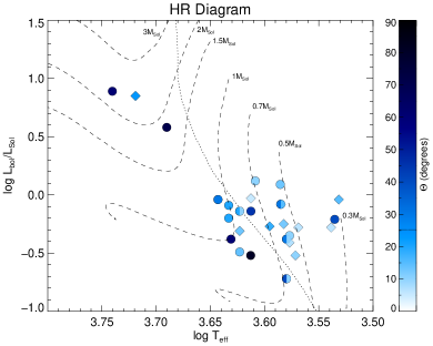
Figure 7: HR diagram with the stars in our sample (filled diamonds) and other stars from the literature (filled circles). Colours represent the stars’ magnetic obliquities. Two colours are used when two different values were found at different epochs. Dashed lines represent mass tracks from pre-main sequence evolutionary models of Tognelli et al. (2011), while the dotted line represents the limit where a radiative core begins to develop, according to these models (stars to the right of this line should be fully convective).

In order to further investigate this hypothesis, we plotted an HR diagram using different colours to represent the magnetic obliquity found for each star (Fig. 7). In a few cases, two different observations using spectropolarimetry resulted in different values of the magnetic obliquity (with differences of up to 30^∘ between the two epochs). Both values are represented in the figure by a two-coloured symbol. We used different symbols to differentiate the sample from our study (filled diamonds) from those taken from the literature (filled circles). Theoretical mass tracks from Tognelli et al. (2011) are also plotted for reference. The dotted line represents the evolutionary phase in which a radiative core is expected to begin to develop, according to Tognelli et al. (2011) (see also Gregory et al., 2012), meaning that stars to the right of this line should be fully convective. This figure seems to suggest that fully convective stars usually have low magnetic obliquities (though there are a few cases where it is as high as 40^∘), while the stars with large magnetic obliquities ($\gtrsim 60^{\circ}$) are those that have developed at least a small radiative core. The average magnetic obliquity among the stars in the fully convective part of the HR diagram is 17^∘ (with an rms dispersion of 12^∘), while in the partly radiative part of the HR diagram it is slightly larger, 35^∘ (with an rms deviation of 22^∘). This could be complementary with other studies of magnetic fields in young stars that suggest that, as a radiative core develops, stellar magnetic fields tend to become more complex and less intense than in fully convective stars (Gregory et al., 2012; Folsom et al., 2016). If this is indeed the case, it may explain why our sample shows a tendency towards low magnetic obliquities, as most of our stars are fully convective.

The apparent evolution of the magnetic field configuration across the HR diagram (in terms of the strength of the field and its complexity, as demonstrated by Folsom et al., 2016; Villebrun et al., 2019, as well as in terms of the magnetic obliquity, as shown here) points to a dynamic origin of stellar magnetic fields, likely as the consequence of a dynamo effect. This study and previous ones such as Folsom et al. (2016) also seem to suggest that there are intrinsic differences between magnetic fields of stars that are fully convective and those that have begun to develop a radiative core.

6 Summary and conclusions

We have analysed the variability of the HeI$\lambda$5876 emission line profile in a sample of 10 CTTSs and 1 WTTS, measured with high-resolution spectroscopy over a period of up to 10 days. Most observations show a simple profile, dominated by a narrow component (NC) that is believed to originate in accretion shocks near the stellar surface. For four stars, the HeI$\lambda$5876 line profile is seen to be composed of a combination of narrow and broad component (BC), the latter being believed to have multiple origins, likely formed in both hot winds and accretion columns (Beristain et al., 2001). For these four stars, each individual observation was fitted with a combination of two Gaussians, one broader than the other, in order to separately investigate the origin of the two components. Both appear to be variable in their own way on the time-scale spanned by our observations. With the resolution of our spectra we can clearly see that the NC is not truly Gaussian, but this approximation does seem to be valid when analysing its radial velocity. This can be illustrated by the fact that, even though the star T Tau’s He I line profile is clearly dominated by the BC, its stellar rotation period of 2.8 days is recovered from the radial velocity measurements of the NC, while this period is not clear in a radial velocity analysis of the composite profile. This shows that an analysis of the NC of the He I line is still possible even for stars whose He I line profile is clearly dominated by the BC.

The NC of the HeI$\lambda$5876 emission line is shown to be redshifted by an average of 6.4 km s^-1 in our sample, with a standard deviation of 1.4 km s^-1. By taking the median redshifts for each star and de-projecting them from our line of sight, we find that the material responsible for this emission is traveling at an average of 9 km s^-1 in our sample (with a standard deviation of 4.3 km s^-1). This velocity is consistent with material tracing the post-shock region of accretion shocks, after considerable deceleration of the free-falling material has occurred.

By measuring the amplitude of the radial velocity variability ($\Delta V_{rad}$) of the NC of the HeI$\lambda$5876 emission line, along with the stars’ projected rotational velocities ($v\sin i$), we were able to estimate these stars’ magnetic obliquities ($\Theta$ - the angle between the axis of their magnetic field and rotation axis). We find an average magnetic obliquity of $11.4^{\circ}$ in our sample, with an rms dispersion of $5.4^{\circ}$. The magnetic axis thus seems close to being aligned with the stellar rotation axis in our sample. This is not entirely in agreement with other studies of magnetic field configurations (e.g., Johnstone et al., 2014), which find several cases of misalignments larger than 20^∘. This difference may simply be due to an issue of low number statistics. However, there is also the possibility that our sample may be subject to a selection bias. With the exception of T Tau, the stars in this sample were chosen on the basis that their He I line profiles are dominated by the NC. The star T Tau, whose He I line profile is clearly dominated by the BC (see Fig. 2), is the star that presents the largest magnetic obliquity in our sample (of $23^{\circ}\pm 10^{\circ}$). If the mechanism that originates the BC of the HeI$\lambda$5876 line is somehow connected to larger magnetic obliquities, then this would result in a selection bias in our sample. However, to confirm this hypothesis, a larger study of magnetic obliquities, including stars with more diverse He I profiles, would be needed.

We find tentative evidence for a trend between the position of a star on the HR diagram and its magnetic obliquity. This result is based on a small sample and should be taken with care, but the possibility that a star’s inner structure can play a strong role in determining its magnetic obliquity would be consistent with other studies that show an apparent evolution of a star’s magnetic field as it evolves across the HR diagram (e.g., Gregory et al., 2012; Folsom et al., 2016; Villebrun et al., 2019). In particular, there may be a considerable difference between the magnetic field configurations of stars that are fully convective and those that are partially radiative, a possibility that merits further investigation as it is unfortunately still subject to low number statistics. If this is indeed the case, it supports the idea that magnetic fields in T Tauri stars are generated by a dynamo, rather than by fossil fields, and that the existence of a boundary between radiative and convective zones plays an important role in determining the geometry of that magnetic field. It could also be responsible for our sample’s bias towards low magnetic obliquities, since most of the stars in our sample are in the fully convective portion of the HR diagram.

Besides our main results, we also find some interesting aspects of individual sources. A joint analysis of the variability of the He I, H$\alpha$ and H$\beta$ lines show, in at least three sources (DK Tau, DN Tau and IP Tau), evidence for a spatial association between the accretion shocks on the stellar surface and the accretion columns, which would be expected in a scenario in which disc-locking takes place. Meanwhile another source, DF Tau, shows evidence for a variable wind that seems to be spatially associated with the accretion shock. This could be a stellar wind that is launched very close to the accretion shock, or it could result from a non-uniform disc wind being launched from close to the truncation radius, in a part of the inner disc where an accretion column is forming. Since this variability seems to be consistent with having the same period as the stellar rotation, this would also be close to the co-rotation radius.

We find that the star IW Tau, previously reported as a non-accreting, weak-line T Tauri star, in fact presents redshifted He I emission, which means that this emission must come from matter falling onto the star. It seems therefore that this star is still weakly accreting. An analysis of the flux of several emission lines that are known to be linked with accretion leads us to estimate a mass accretion rate of $\dot{M}_{acc}=3\times 10^{-10}~{}\mathrm{M}_{\odot}~{}\mathrm{yr}^{-1}$ for this star. We should note that this value is likely overestimated, since at such low limits of accretion, these lines are likely contaminated with a strong contribution from chromospheric activity.

Finally, we recover the stellar rotation period of 2.8 days for the star T Tau in both the radial velocity analysis of the NC of the He I line, as well as in a portion of a 2-dimensional periodogram of this line. However we find a slightly larger period, of 3.1 days, in the wings of this line and in the radial velocity analysis of its BC, which is redshifted. Since the BC in this case is believed to originate from the accretion columns, while the NC originates at the accretion shock near the stellar surface, this may be an indication that there is differential rotation throughout the accretion columns of this system. Although, seeing as the two periods are very similar, this is not enough evidence to conclude this with certainty and further investigation would be needed to support this claim.

Data availability

The data underlying this article can be accessed through the SOPHIE archive at http://atlas.obs-hp.fr/sophie/.

Appendix A Additional figures

The following pages present figures that are discussed in the text (Figs. 8 through 11).

Figure 8: Variability of the radial velocity of the HeI$\lambda 5876$ narrow component, veiling, the HeI$\lambda 5876$ profile, the H$\alpha$ profile and the H$\beta$ profile for the stars in our sample that were observed for only one rotation cycle.

Figure 10: Continued. This time only one plot is shown for each star, since only one rotation period was measured.

Appendix B Additional tables

Table 4 shows the equivalent widths of the He I, H$\alpha$ and H$\beta$ lines in this study. In order to demonstrate the variability of these emission lines, the average and standard deviation over all nights are given. Table 5 shows information on the magnetic obliquities of other T Tauri stars taken from the literature.

Table 4: Equivalent widths of H$\alpha$, H$\beta$ and HeI$\lambda$5876 for our sample.

Star	H$\alpha$		H$\beta$		He I
	<EW>	$\sigma$	<EW>	$\sigma$	<EW>	$\sigma$
DETau	-65	7	-30	4	-1.0	0.2
DFTau	-64	11	-17	6	-2.5	0.7
DKTau	-35	19	-9.5	4.7	-1.1	0.4
DNTau	-7.6	1.0	-3.3	0.5	-0.34	0.08
GITau	-10.3	3.2	-5.0	2.6	-0.54	0.35
GKTau	-21	8	-4.1	2.1	-0.44	0.10
GMAur	-106	5	-16	2	-1.1	0.4
IPTau	-16	6	-7.9	3.1	-0.62	0.37
IWTau	-3.8	0.6	-1.7	0.3	-0.07	0.02
TTau	-98	13	-17	4	-1.0	0.3
V826Tau	-1.5	0.2	-0.27	0.16	-0.07	0.01
V836Tau	-14.2	1.4	-3.4	0.4	-0.22	0.04

Notes: We show the mean equivalent width (<EW>) of each emission line over the several days observations, along with the standard deviation ($\sigma$), in order to illustrate the variability of these lines. All values are given in Å.

Table 5: Magnetic obliquities of other CTTSs from the literature

Star	Spectral type	Mass ($M_{\odot}$)	$\Theta(^{\circ})$	Source of $\Theta$	References
AA Tau	M0.6	0.57	10	ZDI	(Johnstone et al., 2014; Donati et al., 2010b)
BP Tau (Feb 2006)	M0.5	0.62	10	ZDI	(Johnstone et al., 2014; Donati et al., 2008)
BP Tau (Dec 2006)	"	"	30	ZDI	(Johnstone et al., 2014; Donati et al., 2008)
CI Tau	K5.5	0.90	20	ZDI	(Donati et al., 2020)
CR Cha	K2	2.00	70	ZDI	(Johnstone et al., 2014; Hussain et al., 2009)
CV Cha	G8	1.05	60	ZDI	(Johnstone et al., 2014; Hussain et al., 2009)
DN Tau (2010)	M0.3	0.55	30	ZDI	(Donati et al., 2013)
DN Tau (2012)	"	"	15	ZDI	(Donati et al., 2013)
GQ Lup (2009)	K5.0	0.89	30	ZDI	(Johnstone et al., 2014; Donati et al., 2012)
GQ Lup (2011)	"	"	30	ZDI	(Johnstone et al., 2014; Donati et al., 2012)
LkCa 15	K5.5	0.89	20	ZDI	(Donati et al., 2019)
TW Hya (2008)	M0.5	0.69	40	ZDI	(Johnstone et al., 2014; Donati et al., 2011b)
TW Hya (2010)	"	"	10	ZDI	(Johnstone et al., 2014; Donati et al., 2011b)
V2129 Oph (2005)	K6	1.35	20	ZDI	(Johnstone et al., 2014; Donati et al., 2007)
V2129 Oph (2009)	"	"	10	ZDI	(Johnstone et al., 2014; Donati et al., 2011a)
V2247 Oph	M1	0.36	40	ZDI	(Johnstone et al., 2014; Donati et al., 2010a)
V4046 Sgr A	K5	0.95	60	ZDI	(Johnstone et al., 2014; Donati et al., 2011c)
V4046 Sgr B	K5	0.85	80	ZDI	(Johnstone et al., 2014; Donati et al., 2011c)
DR Tau	K6	0.88	14	$\Delta V_{r}(HeI)$	(Petrov et al., 2011)
EX Lup	M0	0.60	13	$\Delta V_{r}(HeI)$	(Sicilia-Aguilar et al., 2015)
RU Lup	K7	0.65	10	$\Delta V_{r}(HeI)$	(Gahm et al., 2013; Alcalá et al., 2017)
RW Aur A	K6.5	1.13	45	Modeling spectral variability	(Petrov et al., 2001)

Notes: To maintain consistency with this work, for the star EX Lup we took the value of $\Theta$ derived from the amplitude of the radial velocity variability of the HeI$\lambda 5876$ line. Masses and spectral types are from Herczeg & Hillenbrand (2014), where available. For the stars not included in that study, masses were re-derived using the same mass tracks they used (the PISA tracks, Tognelli et al., 2011), in order to maintain consistency among the sample.

References

- Akeson et al. (2019) Akeson R. L., Jensen E. L. N., Carpenter J., Ricci L., Laos S., Nogueira N. F., Suen-Lewis E. M., 2019, ApJ, 872, 158
- Alcalá et al. (2017) Alcalá J. M., et al., 2017, A&A, 600, A20
- Alencar et al. (2010) Alencar S. H. P., et al., 2010, A&A, 519, A88
- Alencar et al. (2018) Alencar S. H. P., et al., 2018, A&A, 620, A195
- Appenzeller et al. (1986) Appenzeller I., Jankovics I., Jetter R., 1986, A&AS, 64, 65
- Artemenko et al. (2012) Artemenko S. A., Grankin K. N., Petrov P. P., 2012, Astronomy Letters, 38, 783
- Beckwith et al. (1990) Beckwith S. V. W., Sargent A. I., Chini R. S., Guesten R., 1990, AJ, 99, 924
- Beristain et al. (2001) Beristain G., Edwards S., Kwan J., 2001, ApJ, 551, 1037
- Bessolaz et al. (2008) Bessolaz N., Zanni C., Ferreira J., Keppens R., Bouvier J., 2008, A&A, 478, 155
- Blinova et al. (2016) Blinova A. A., Romanova M. M., Lovelace R. V. E., 2016, MNRAS, 459, 2354
- Boisse et al. (2010) Boisse I., et al., 2010, A&A, 523, A88
- Bouchy et al. (2009) Bouchy F., et al., 2009, A&A, 505, 853
- Bouvier et al. (1993) Bouvier J., Cabrit S., Fernandez M., Martin E. L., Matthews J. M., 1993, A&AS, 101, 485
- Bouvier et al. (1995) Bouvier J., Covino E., Kovo O., Martin E. L., Matthews J. M., Terranegra L., Beck S. C., 1995, A&A, 299, 89
- Bouvier et al. (2007) Bouvier J., et al., 2007, A&A, 463, 1017
- Calvet & Gullbring (1998) Calvet N., Gullbring E., 1998, ApJ, 509, 802
- Crockett et al. (2012) Crockett C. J., Mahmud N. I., Prato L., Johns-Krull C. M., Jaffe D. T., Hartigan P. M., Beichman C. A., 2012, ApJ, 761, 164
- Dodin & Lamzin (2012) Dodin A. V., Lamzin S. A., 2012, Astrononmy Letters, 38, 649
- Donati et al. (1997) Donati J.-F., Semel M., Carter B. D., Rees D. E., Cameron A. C., 1997, MNRAS, 291, 658
- Donati et al. (2007) Donati J. F., et al., 2007, MNRAS, 380, 1297
- Donati et al. (2008) Donati J.-F., et al., 2008, MNRAS, 386, 1234
- Donati et al. (2010a) Donati J.-F., et al., 2010a, MNRAS, 402, 1426
- Donati et al. (2010b) Donati J.-F., et al., 2010b, MNRAS, 409, 1347
- Donati et al. (2011a) Donati J.-F., et al., 2011a, MNRAS, 412, 2454
- Donati et al. (2011b) Donati J.-F., et al., 2011b, MNRAS, 417, 472
- Donati et al. (2011c) Donati J. F., et al., 2011c, MNRAS, 417, 1747
- Donati et al. (2012) Donati J.-F., et al., 2012, MNRAS, 425, 2948
- Donati et al. (2013) Donati J.-F., et al., 2013, MNRAS, 436, 881
- Donati et al. (2019) Donati J. F., et al., 2019, MNRAS, 483, L1
- Donati et al. (2020) Donati J. F., et al., 2020, MNRAS, 491, 5660
- Duchêne et al. (2005) Duchêne G., Ghez A. M., McCabe C., Ceccarelli C., 2005, ApJ, 628, 832
- Dupree et al. (2012) Dupree A. K., et al., 2012, ApJ, 750, 73
- Folsom et al. (2016) Folsom C. P., et al., 2016, MNRAS, 457, 580
- Furlan et al. (2005) Furlan E., et al., 2005, ApJ, 628, L65
- Gahm et al. (2013) Gahm G. F., Stempels H. C., Walter F. M., Petrov P. P., Herczeg G. J., 2013, A&A, 560, A57
- Gregory et al. (2012) Gregory S. G., Donati J.-F., Morin J., Hussain G. A. J., Mayne N. J., Hillenbrand L. A., Jardine M., 2012, ApJ, 755, 97
- Hamann & Persson (1992) Hamann F., Persson S. E., 1992, ApJS, 82, 247
- Hartigan et al. (1989) Hartigan P., Hartmann L., Kenyon S., Hewett R., Stauffer J., 1989, ApJS, 70, 899
- Herczeg & Hillenbrand (2014) Herczeg G. J., Hillenbrand L. A., 2014, ApJ, 786, 97
- Hussain et al. (2009) Hussain G. A., et al., 2009, MNRAS, 398, 189
- Johnstone et al. (2014) Johnstone C. P., Jardine M., Gregory S. G., Donati J.-F., Hussain G., 2014, MNRAS, 437, 3202
- Joy (1945) Joy A. H., 1945, ApJ, 102, 168
- Joy (1949) Joy A. H., 1949, ApJ, 110, 424
- Köhler et al. (2000) Köhler R., Kasper M., Herbst T., 2000, in IAU Symposium. p. 63
- Koresko (2000) Koresko C. D., 2000, ApJ, 531, L147
- Kurosawa & Romanova (2013) Kurosawa R., Romanova M. M., 2013, MNRAS, 431, 2673
- Kurosawa et al. (2011) Kurosawa R., Romanova M. M., Harries T. J., 2011, MNRAS, 416, 2623
- Long et al. (2018) Long F., et al., 2018, ApJ, 869, 17
- Manara et al. (2019) Manara C. F., et al., 2019, A&A, 628, A95
- McGinnis et al. (2015) McGinnis P. T., et al., 2015, A&A, 577, A11
- Melo et al. (2001) Melo C. H. F., Pasquini L., De Medeiros J. R., 2001, A&A, 375, 851
- Percy et al. (2010) Percy J. R., Grynko S., Seneviratne R., Herbst W., 2010, PASP, 122, 753
- Perruchot et al. (2008) Perruchot S., et al., 2008, in Proc. SPIE. p. 70140J, doi:10.1117/12.787379
- Petrov et al. (2001) Petrov P. P., Gahm G. F., Gameiro J. F., Duemmler R., Ilyin I. V., Laakkonen T., Lago M. T. V. T., Tuominen I., 2001, A&A, 369, 993
- Petrov et al. (2011) Petrov P. P., Gahm G. F., Stempels H. C., Walter F. M., Artemenko S. A., 2011, A&A, 535, A6
- Piétu et al. (2014) Piétu V., Guilloteau S., Di Folco E., Dutrey A., Boehler Y., 2014, A&A, 564, A95
- Press et al. (1992) Press W. H., Teukolsky S. A., Vetterling W. T., Flannery B. P., 1992, Numerical recipes in FORTRAN. The art of scientific computing, 2nd edn. Cambridge: University Press
- Rebull et al. (2020) Rebull L. M., Stauffer J. R., Cody A. M., Hillenbrand L. A., Bouvier J., Roggero N., David T. J., 2020, Rotation of Low-Mass Stars in Taurus with K2, Accepted by AJ (arXiv:2004.04236)
- Richichi et al. (1994) Richichi A., Leinert C., Jameson R., Zinnecker H., 1994, A&A, 287, 145
- Romanova et al. (2002) Romanova M. M., Ustyugova G. V., Koldoba A. V., Lovelace R. V. E., 2002, ApJ, 578, 420
- Romanova et al. (2013) Romanova M. M., Ustyugova G. V., Koldoba A. V., Lovelace R. V. E., 2013, MNRAS, 430, 699
- Rydgren et al. (1976) Rydgren A. E., Strom S. E., Strom K. M., 1976, ApJS, 30, 307
- Rydgren et al. (1984) Rydgren A. E., Zak D. S., Vrba F. J., Chugainov P. F., Zajtseva G. V., 1984, AJ, 89, 1015
- Shu et al. (1994) Shu F., Najita J., Ostriker E., Wilkin F., Ruden S., Lizano S., 1994, ApJ, 429, 781
- Sicilia-Aguilar et al. (2015) Sicilia-Aguilar A., Fang M., Roccatagliata V., Cameron A. C., Kospal A., Henning T., Abraham P., Sipos N., 2015, A&A, 580, A82
- Sicilia-Aguilar et al. (2017) Sicilia-Aguilar A., et al., 2017, A&A, 607, A127
- Simon et al. (2017) Simon M., et al., 2017, ApJ, 844, 158
- Stauffer et al. (2014) Stauffer J., et al., 2014, AJ, 147, 83
- Stauffer et al. (2016) Stauffer J., et al., 2016, AJ, 151, 60
- Tognelli et al. (2011) Tognelli E., Prada Moroni P. G., Degl’Innocenti S., 2011, A&A, 533, A109
- Tripathi et al. (2017) Tripathi A., Andrews S. M., Birnstiel T., Wilner D. J., 2017, ApJ, 845, 44
- Villebrun et al. (2019) Villebrun F., et al., 2019, A&A, 622, A72
- White & Basri (2003) White R. J., Basri G., 2003, ApJ, 582, 1109
- Wolk & Walter (1996) Wolk S. J., Walter F. M., 1996, AJ, 111, 2066