Mixture of linear experts model for censored data:
A novel approach with scale-mixture of normal distributions

Abstract

The classical mixture of linear experts (MoE) model is one of the widespread statistical frameworks for modeling, classification, and clustering of data. Built on the normality assumption of the error terms for mathematical and computational convenience, the classical MoE model has two challenges: 1) it is sensitive to atypical observations and outliers, and 2) it might produce misleading inferential results for censored data. The paper is then aimed to resolve these two challenges, simultaneously, by proposing a novel robust MoE model for model-based clustering and discriminant censored data with the scale-mixture of normal class of distributions for the unobserved error terms. Based on this novel model, we develop an analytical expectation-maximization (EM) type algorithm to obtain the maximum likelihood parameter estimates. Simulation studies are carried out to examine the performance, effectiveness, and robustness of the proposed methodology. Finally, real data is used to illustrate the superiority of the new model.

1 Introduction

The issue of model-based clustering has recently received considerable attention in statistics with applications in medical sciences, public health and engineering as shown in Feigelson and Babu (2012); Wang et al. (2019); Shafiei et al. (2020). The grouping structure identification in the data usually provides informative results for solving real-world problems. One of the most acknowledged statistical tools for model-based clustering is the finite mixture (FM) model. The FM model, initially introduced by Redner and Walker (1984), is a convex linear combination of the probability density functions (pdf) given by

$$f(y;\bm{\Theta})=\sum_{j=1}^{G}\pi_{j}\;g(y;\bm{\theta}_{j}),$$

where $G$ is the total number of clusters, $\pi_{j}$’s are the mixing proportions subjected to $\sum_{j=1}^{G}\pi_{j}=1$, $g(\cdot;\bm{\theta}_{j})$ is the associated pdf of the $j$th underlying mixing component parametrized by $\bm{\theta}_{j}$, and $\bm{\Theta}=(\bm{\theta}_{1},\ldots,\bm{\theta}_{G},\pi_{1},\ldots,\pi_{G-1})$. The mixing proportion is, in fact, $\pi_{j}=Pr(Z^{\ast}=j)$ where the hidden categorical random variable $Z^{*}$ indicates from which component each observation is arisen. Upon the normality and/or non-normality assumptions for the mixing components, various FM models have recently been introduced for modeling heterogeneous data. They have widely been employed in scientific studies such as genetics, image processing, medicine, economics and astronomy, for example in Wang et al. (2018); Punzo et al. (2018); Sugasawa et al. (2018); Naderi et al. (2017a, 2019); Tomarchio and Punzo (2019); Morris et al. (2019) to name a few recently published papers.

In the context of regression analysis, the FM models are also found appealing applications to investigate the relationship between the random phenomena under study arisen from various unknown latent homogeneous groups. Specifically, the FM regression model relies on the assumption that the pdf of underlying distribution is

$$f(y;\bm{\Theta})=\sum_{j=1}^{G}\pi_{j}g(y-\bm{x}^{\top}\bm{\beta}_{j};\bm{\theta}_{j}),$$

where $\bm{x}=(1,x_{1},\ldots,x_{p-1})^{\top}\in\mathbb{R}^{p}$ is the vector of $p$ explanatory variables corresponding to response $y$, and $\bm{\beta}_{j}=(\beta_{j0},\ldots,\beta_{j(p-1)})^{\top}$, denotes the regression coefficients of the $j$th component. In this regard, Liu and Lin (2014) proposed the skew-normal mixture regression model by considering the pdf of skew-normal distribution as the mixing component and applied it to the physiological data to illustrate its utility. Hu et al. (2017) introduced FM regression model by assuming that the components have log-concave error densities and developed two EM-type (Dempster et al., 1977) algorithms to obtain the maximum likelihood (ML) parameter estimates. Lamont et al. (2016) also investigated the effect of modeling covariance between independent variables and latent classes on the fitting/clustering results.

Built up from this FM regression model, the MoE model (Jacobs et al., 1991) is perhaps one of the most acknowledged approaches in the statistics and machine learning fields. Although the MoE and FM regression models share similar structure, they differ in many aspects. In formulation of the MoE model, it is assumed that both mixing proportions and component densities conditionally depend on some input covariates. More precisely, let $Y\in\mathbb{R}$ be the response variable, $\bm{x}\in\mathbb{R}^{p}$ and $\bm{r}=(1,r_{1},\ldots,r_{q-1})^{\top}\in\mathbb{R}^{q}$ are the vector of explanatory and covariate values corresponding to $Y$. Instead of considering constant mixing component in FM regression model, the MoE model assumes that $\pi_{j}$ to be modeled as a function (generally logistic or softmax function) of input $\bm{r}$, known as a gating function. For instance, the pdf of the normal-based MoE (MoE-N) is

$$f(y;\bm{\Theta})=\sum_{j=1}^{G}\pi_{j}(\bm{r};\bm{\tau})\phi(y;\bm{x}^{\top}\bm{\beta}_{j},\sigma_{j}^{2}),$$ (1)

where $\phi(\cdot,\mu,\sigma^{2})$ is the pdf of normal distribution with the location and scale parameters $\mu$ and $\sigma^{2}$, $\mathcal{N}(\mu,\sigma^{2})$, for gating parameters $\bm{\tau}=(\bm{\tau}_{1}^{\top},\ldots,\bm{\tau}_{G-1}^{\top})^{\top}$ with $\bm{\tau}_{j}=(\tau_{j0},\ldots,\tau_{j(q-1)})^{\top}$,

$$\pi_{j}(\bm{r};\bm{\tau})=Pr(Z^{*}=j|\bm{r})=\frac{\exp\{\bm{\tau}_{j}^{\top}\bm{r}\}}{1+\sum_{l=1}^{G-1}\exp\{\bm{\tau}_{l}^{\top}\bm{r}\}},$$ (2)

and for $\bm{\theta}_{j}=(\bm{\beta}_{j},\sigma^{2}_{j})$, the model parameters set is $\bm{\Theta}=(\bm{\theta}_{1},\ldots,\bm{\theta}_{G},\bm{\tau})$. It should be emphasized that $\bm{x}$ and $\bm{r}$ can be exactly or partially identical. Since the introduction of the MoE-N model, considerable amount of contributions have been produced to overcome its potential deficiency in analyzing skew and heavy-tail distributed data. See for instance the works by Nguyen and McLachlan (2016); Chamroukhi (2016, 2017) on proposing the Laplace, Student-$t$ and skew-$t$ MoE models, respectively.

In many practical situations, such as economic and clinical studies, medical research and epidemiological cancer studies, the data are collected under some imposed detection limits. It might lead to incomplete data with different types of interval, left and/or right-censored responses. In this regard, censored regression model with the normality assumption for the error terms, known as Tobit model, was constructed by Tobin (1958). Since then, the extensions of Tobit model have been introduced by researchers to draw robust inference from censored data. For instance, using the scale-mixture of normal (SMN) class of distributions for the error terms, Garay et al. (2016, 2017) presented the nonlinear and linear censored regression models to overcome the problem of atypical observations in the data. Mattos et al. (2018) also proposed censored linear regression model with the scale-mixture of skew-normal class of distributions to accommodate asymmetrically distributed censored datasets. Moreover, mixture of censored regression models based on the Student-$t$ model and on the SMN class of distributions were proposed by Lachos et al. (2019); Zeller et al. (2018) as a flexible approach for modeling multimodal censored data with fat tails.

Extending the proven proficiency of the MoE model in statistical applications, the main objective of the current paper is to propose a MoE model based on the SMN class of distributions for censored data, hereafter referred as “MoE-SMN-CR model”. Due to the computational complexity, we develop an innovative EM-type algorithm to obtain the ML parameter estimates. The associated variance-covariance matrix of the ML estimators is also approximated by an information-based approach. To illustrate the computational aspects and practical performance of the proposed methodology, a real data analysis and several simulation studies are presented.

The remainder of the paper is organized as follows. Section 2 briefly reviews the SMN class of distributions. Model formulation and parameter estimation procedure of the MoE-SMN-CR model are presented in Section 3. Four simulation studies are conducted in Section 4 to check the asymptotic properties of the ML estimates as well as to investigate the performance of the proposed model. The applicability of the proposed method is illustrated in Section 5 by analyzing wage-rates dataset. Finally, we conclude the paper with a discussion and suggestions for future work in Section 6.

2 An overview on the scale-mixture of normal class of distributions

A random variable $Y$ follows an scale-mixture of normal (SMN) distribution, denoted by $\mathcal{SMN}(\mu,\sigma^{2},\bm{\nu})$, if it is generated by

$$Y=\mu+U^{-1/2}V,\qquad V\perp U,$$ (3)

where $V\sim\mathcal{N}(0,\sigma^{2})$, $U$ (scale mixture factor) is a positive random variable with the cumulative distribution function (cdf) $H(\cdot;\bm{\nu})$, and the symbol $\perp$ indicates independence. Referring to (3), the hierarchical representation of the SMN class of distributions can be written as

$$Y|U=u\sim N(\mu,u^{-1}\sigma^{2}),\qquad U\sim H(u;\bm{\nu}),$$ (4)

accordingly, the pdf of the random variable $Y$ is obtained as

$$f_{{}_{\text{SMN}}}(y;\mu,\sigma^{2},\bm{\nu})=\int_{0}^{\infty}\phi(y;\mu,u^{-1}\sigma^{2})\;dH(u;\bm{\nu}),\qquad y\in\mathbb{R}.$$

In what follows, $f_{{}_{\text{SMN}}}(\cdot;\bm{\nu})$ and $F_{{}_{\text{SMN}}}(\cdot;\bm{\nu})$ will be used to denote the pdf and cdf of the standard SMN distribution ($\mu=0,\sigma^{2}=1$). With different specifications of the distribution of $U$, many special cases of the general SMN class of distributions can be obtained. We focus on a few commonly used examples of the SMN class of distributions in this paper:

• Normal (N) distribution: The SMN class of distributions contains the normal model as $U=1$ with probability one.

• Student-$t$ (T) distribution: If $U\sim Gamma({\nu}/{2},{\nu}/{2})$, where $Gamma(\alpha,\beta)$ represents the gamma distribution with shape and scale parameters $\alpha$ and $\beta$, respectively, the random variable $Y$ then follows the Student-$t$ distribution, $Y\sim\mathcal{T}(\mu,\sigma^{2},\nu)$. For $\nu=1$ the Student-$t$ distribution turns into the Cauchy distribution which has no defined mean and variance.

• Slash (SL) distribution: Let $U$ in (3) follows $Beta(\nu,1)$, where $Beta(a,b)$ signifies the beta distribution with parameter $a$ and $b$. Then, $Y$ distributed as a slash model, denoted by $Y\sim\mathcal{SL}(\mu,\sigma^{2},\nu)$, with pdf

  $$f_{{}_{\text{SL}}}(y;\mu,\sigma^{2},\nu)=\nu\int_{0}^{1}u^{\nu-1}\phi(y;\mu,u^{-1}\sigma^{2})\;du,\qquad y\in\mathbb{R}.$$

• Contaminated-normal (CN) distribution: Let $U$ be a discrete random variable with pdf

  $$h(u;\nu,\gamma)=\nu\mathbb{I}_{\gamma}(u)+(1-\nu)\mathbb{I}_{1}(u),\qquad\nu,\gamma\in(0,1),$$

  where $\mathbb{I}_{A}(\cdot)$ represents the indicator function of the set $A$. The random variable $Y$ in (3) then follows the contaminated-normal distribution, $Y\sim\mathcal{CN}(\mu,\sigma^{2},\nu,\gamma)$, which has the pdf

  $$f_{{}_{\text{CN}}}(y;\mu,\sigma^{2},\nu,\gamma)=\nu\phi(y;\mu,\gamma^{-1}\sigma^{2})+(1-\nu)\phi(y;\mu,\sigma^{2}),\qquad y\in\mathbb{R}.$$

  Note that in the pdf of CN distribution, the parameter $\nu$ denotes the proportion of outliers (bad points) and $\gamma$ is the contamination factor.

More technical details and information of the SMN distribution family, used for the calculation of some conditional expectations involved in the proposed EM-type algorithm, are provided in the A with proof in Garay et al. (2017). We will refer to the MoE model of censored data based on the special cases of the SMN class of distributions as MoE-N-CR, MoE-T-CR, MoE-SL-CR and MoE-CN-CR for the normal, Student-$t$, slash and contaminated-normal cases, respectively.

3 The scale-mixture of normal censored mixture of linear experts model

3.1 Model specification

Extending the classical MoE model with normal distribution in model (1), we consider the expert components formulated by the SMN class of distributions. Therefore, the resulting pdf, in which the polynomial regression and multinomial logistic model are used for the components and mixing proportions, can be defined as

$$f(y_{i};\bm{\Theta})=\sum_{j=1}^{G}\pi_{j}(\bm{r}_{i};\bm{\tau})f_{{}_{\text{SMN}}}(y_{i};\bm{x}_{i}^{\top}\bm{\beta}_{j},\sigma_{j}^{2},\bm{\nu}_{j}),\quad\quad i=1,\ldots,n,$$ (5)

where $\bm{Y}=(Y_{1},\ldots,Y_{n})^{\top}$ is the vector of response variables, $\bm{x}_{i}$ and $\bm{r}_{i}$ are the vector of explanatory and covariate variables corresponding to $Y_{i}$, $\pi_{j}(\cdot;\bm{\tau})$ is defined in (2), and for $\bm{\theta}_{j}=(\bm{\beta}_{j},\sigma^{2}_{j},\bm{\nu}_{j})$ the model parameters is $\bm{\Theta}=(\bm{\theta}_{1},\ldots,\bm{\theta}_{G},\bm{\tau})$.

In the MoE-SMN-CR model, we assume that the response variables are partially observed. In other word, we suppose some of the response variables are suffering from a type of censoring, that could be interval-, left- or right-censoring. Thus, let the available response variable $Y_{i}$ be presented as the joint variables $(W_{i},\rho_{i})$ where $W_{i}$ represents the uncensored reading $(W_{i}=Y_{Oi})$ or interval-censoring $(W_{i}=(C_{i1},C_{i2}))$ and $\rho_{i}$ is the censoring indicator: $\rho_{i}=1$ if $C_{i1}\leq Y_{i}\leq C_{i2}$ and $\rho_{i}=0$ if $Y_{i}=Y_{Oi}$. Note that in this setting if $C_{i1}=-\infty$ (or $C_{i2}=+\infty$) the left-censoring (or right-censoring) is occurred and in the case $-\infty\neq C_{i1}<C_{i2}\neq+\infty$ the interval-censored realization is observed. We establish our methodology based on the interval-censoring scheme, however, the left/right-censoring schemes are also investigated in the simulation and real-data analyses.

The aforementioned setting leads to divide $\bm{Y}$ to the sets of observed responses and censored cases. Hence, $\bm{Y}$ can be viewed as the latent variable since it is partially unobserved. Under these assumptions, the log-likelihood function of the MoE-SMN-CR model can be written as

$$\ell(\bm{\Theta}|\bm{w},\bm{\rho})=\sum_{i=1}^{n}\log\sum_{j=1}^{G}\pi_{j}(\bm{r}_{i};\bm{\tau})\left[{\sigma_{j}}^{-1}f_{{}_{\text{SMN}}}\left(\frac{w_{i}-\bm{x}_{i}^{\top}\bm{\beta}_{j}}{\sigma_{j}};\bm{\nu}_{j}\right)\right]^{1-\rho_{i}}\left[F_{{}_{\text{SMN}}}\left(\frac{c_{i2}-\bm{x}_{i}^{\top}\bm{\beta}_{j}}{\sigma_{j}};\bm{\nu}_{j}\right)-F_{{}_{\text{SMN}}}\left(\frac{c_{i1}-\bm{x}_{i}^{\top}\bm{\beta}_{j}}{\sigma_{j}};\bm{\nu}_{j}\right)\right]^{\rho_{i}},$$ (6)

where $\bm{w}=(w_{1},\ldots,w_{n})^{\top}$ and $\bm{\rho}=(\rho_{1},\ldots,\rho_{n})^{\top}$ denote the realizations of $\bm{W}=(W_{1},\ldots,W_{n})^{\top}$ and $\bm{\rho}=(\rho_{1},\ldots,\rho_{n})^{\top}$, respectively.

Due to complexity of the log-likelihood (6), there is no analytical solution to obtain the ML estimate of parameters and therefore a numerical search algorithm should be developed. With the embedded hierarchical representation (4), an innovative EM-type algorithm is developed to obtain the ML estimate for the MoE-SMN-CR model.

3.2 EM-based maximum likelihood parameter estimation

Starting from (5) and defining the component label vector $\bm{Z}_{i}=(Z_{i1},\ldots,Z_{iG})^{\top}$ in such a way that the binary latent component-indicators $Z_{ij}=1$ if and only if $Z_{i}^{*}=j$, we have

$$Y_{i}|{Z}_{ij}=1\sim\mathcal{SMN}(\bm{x}_{i}^{\top}\bm{\beta}_{j},\sigma_{j}^{2},\bm{\nu}_{j}),\quad\quad i=1,\ldots,n.$$

Now using (4), the hierarchical representation of the MoE-SMN-CR model is

$$Y_{i}|(\bm{x}_{i},U=u_{i},{Z}_{ij}=1) \sim\mathcal{N}(\bm{x}_{i}^{\top}\bm{\beta}_{j},u_{i}^{-1}\sigma_{j}^{2}),$$

$$U_{i}|Z_{ij}=1 \sim H(\cdot;\bm{\nu}_{j}),$$

$$Z_{i}|\bm{r}_{i} \sim\mathcal{M}\left(1;\pi_{1}(\bm{r}_{i},\bm{\tau}),\ldots,\pi_{G}(\bm{r}_{i},\bm{\tau})\right).$$

where $\mathcal{M}(1;\cdot)$ denotes the one trail multinomial distribution. For the realizations $\bm{y}=(y_{1},\ldots,y_{n})^{\top}$, $\bm{Z}=(\bm{Z}_{1}^{\top},\ldots,\bm{Z}_{n}^{\top})^{\top}$ and the latent values $\bm{u}=(u_{1},\ldots,u_{n})^{\top}$, the log-likelihood function for $\bm{\Theta}$ associated with complete data $\bm{y}_{c}=(\bm{w}^{\top},\bm{\rho}^{\top},\bm{y}^{\top},\bm{u}^{\top},\bm{Z}^{\top})^{\top}$, is therefore given by

$$\ell_{c}(\bm{\Theta}|\bm{y}_{c})=c+\sum_{i=1}^{n}\sum_{j=1}^{G}Z_{ij}\left\{\log\pi_{j}(\bm{r}_{i};\bm{\tau})-\frac{1}{2}\log\sigma_{j}^{2}-\frac{u_{i}}{2\sigma_{j}^{2}}(y_{i}-\bm{x}_{i}^{\top}\bm{\beta}_{j})^{2}+\log h(u_{i};\bm{\nu}_{j})\right\},$$ (7)

where $h(\cdot;\bm{\nu}_{j})$ is the pdf of $U_{i}|Z_{ij}=1$ and $c$ is an additive constant.

We then develop an expectation conditional maximization either (ECME; Liu and Rubin (1994)) algorithm to estimate parameters from the MoE-SMN-CR model. The ECME algorithm is an extension of expectation conditional maximization (ECM; Meng and Rubin (1993)) that not only inherits its stable properties (e.g. monotone convergence and implementation simplicity) but also can be faster than ECM. The iterative ECME algorithm replaces some CM-steps of the ECM with the CML-steps that maximize the corresponding contained log-likelihood function instead. The ECME algorithm for ML estimation of the MoE-SMN-CR model proceeds as follows:

• Initialization: Set the number of iteration to $k=0$ and choose a relative starting point. Due to the multimodal log-likelihood function in the FM and MoE models, the EM-type algorithm for obtaining parameter estimates might not give the global estimates if the initial points depart too far from the real values. Therefore, the choice of initialization process for the EM-based algorithms constitutes an fundamental issue. Nguyen and McLachlan (2016) suggested the starting points for the Laplace MoE model via a modified version of the randomized initial assignment method (McLachlan and Peel, 2000). However, we recommend the following straightforward steps for obtaining the starting points of the MoE-SMN-CR model.

  • Partition the sample into $G$ groups using either $K$-means clustering algorithm (Hartigan and Wong, 1979), $k$-medoids (Kaufman and Rousseeuw, 1990) or trim-$k$-means (Cuesta-Albertos et al., 1997) methods.

  • To initialize $\bm{\tau}^{(0)}$, two strategies can be adopted. As the first and simplest strategy, one can set $\bm{\tau}^{(0)}=\bm{0}$. We note that by using this setting, the MoE model reduces to the FM regression model as a special case. In the second strategy, the information of grouping indices obtained from (i) can be used for initializing $\bm{\tau}$. Based on the grouping indices, one can fit the generalized linear model to the data and compute $\bm{\tau}^{(0)}$.

  • By utilizing the grouping indices of (i), the least squares method is applied to the $j$th group to obtain $\bm{\beta}_{j}^{(0)}$. Moreover, the standard deviation of residuals is used to initialize $\sigma^{(0)}$.

  • Since the normal model belongs to the SMN class of distributions, we adapt $\bm{\nu}_{j}^{(0)}$ corresponds to an initial assumption near normality. For instance, we set $\nu_{j}=20$ in the MoE-T-CR and MoE-SL-CR models.

• E-Step: At the iteration $k$, the expected value of the complete-data log-likelihood function (7), known as the $Q$-function, is

  $$Q(\bm{\Theta}|\bm{\Theta}^{(k)})= \sum_{i=1}^{n}\sum_{j=1}^{G}\hat{z}_{ij}^{(k)}\left\{\log\pi_{j}(\bm{r}_{i};\bm{\tau})-\frac{1}{2}\log\sigma_{j}^{2}-\frac{1}{2\sigma_{j}^{2}}\left(\widehat{uy^{2}}_{ij}^{(k)}+(\bm{x}_{i}^{\top}\bm{\beta}_{j})^{2}\hat{u}_{ij}^{(k)}-2\widehat{uy}_{ij}^{(k)}\bm{x}_{i}^{\top}\bm{\beta}_{j}\right)+\hat{\Upsilon}_{ij}^{(k)}\right\},$$ (8)

  where $\hat{z}_{ij}^{(k)}=E(Z_{ij}|w_{i},\rho_{i},\hat{\bm{\theta}}_{j}^{(k)})$, $\widehat{uy^{2}}_{ij}^{(k)}=E(U_{i}Y_{i}^{2}|w_{i},\rho_{i},\hat{\bm{\theta}}_{j}^{(k)}),$ $\hat{u}_{ij}^{(k)}=E(U_{i}|w_{i},\rho_{i},\hat{\bm{\theta}}_{j}^{(k)}),$ $\widehat{uy}_{ij}^{(k)}=E(U_{i}Y_{i}|w_{i},\rho_{i},\hat{\bm{\theta}}_{j}^{(k)}),$ and $\hat{\Upsilon}_{ij}^{(k)}=E\big{(}\log h(U_{i};\bm{\nu}_{j})|w_{i},\rho_{i},\hat{\bm{\theta}}_{j}^{(k)}\big{)}$. In what follows, we discuss about the computation of conditional expectations for both uncensored and censored cases.

  • For the uncensored observations, we have $\rho_{i}=0$ and so, $\hat{u}_{ij}^{(k)}=E(U_{i}|Y=y_{i},\hat{\bm{\theta}}_{j}^{(k)})$, $\widehat{uy}_{ij}^{(k)}=y_{i}\hat{u}_{ij}^{(k)},$ $\widehat{uy^{2}}_{ij}^{(k)}=y_{i}^{2}\hat{u}_{ij}^{(k)},$

    $$\hat{z}_{ij}^{(k)}=\frac{\pi_{j}(\bm{r}_{i};\hat{\bm{\tau}}^{(k)})f_{{}_{\text{SMN}}}\left(y_{i};\bm{x}_{i}^{\top}\hat{\bm{\beta}}_{j}^{(k)},\hat{\sigma}_{j}^{2(k)},\hat{\bm{\nu}}_{j}^{(k)}\right)}{\sum_{l=1}^{G}\pi_{l}(\bm{r}_{i};\hat{\bm{\tau}}^{(k)})f_{{}_{\text{SMN}}}\left(y_{i};\bm{x}_{i}^{\top}\hat{\bm{\beta}}_{l}^{(k)},\hat{\sigma}_{l}^{2(k)},\hat{\bm{\nu}}_{l}^{(k)}\right)},\qquad\hat{\Upsilon}_{ij}^{(k)}=E\big{(}\log h(U_{i};\bm{\nu}_{j})|Y=y_{i},\hat{\bm{\theta}}_{j}^{(k)}\big{)}.$$

  • For the censored case which is $\rho_{i}=1$, we have

    $$\hat{z}_{ij}^{(k)} =E(Z_{ij}|c_{i1}\leq Y_{i}\leq c_{i2},\hat{\bm{\theta}}_{j}^{(k)})=\frac{\pi_{j}(\bm{r}_{i};\hat{\bm{\tau}}^{(k)})\left[F_{{}_{\text{SMN}}}\left(\frac{c_{i2}-\bm{x}_{i}^{\top}\hat{\bm{\beta}}_{j}^{(k)}}{\hat{\sigma}_{j}^{(k)}};\hat{\bm{\nu}}_{j}^{(k)}\right)-F_{{}_{\text{SMN}}}\left(\frac{c_{i1}-\bm{x}_{i}^{\top}\hat{\bm{\beta}}_{j}^{(k)}}{\hat{\sigma}_{j}^{(k)}};\hat{\bm{\nu}}_{j}^{(k)}\right)\right]}{\sum_{l=1}^{G}\pi_{l}(\bm{r}_{i};\hat{\bm{\tau}}^{(k)})\left[F_{{}_{\text{SMN}}}\left(\frac{c_{i2}-\bm{x}_{i}^{\top}\hat{\bm{\beta}}_{l}^{(k)}}{\hat{\sigma}_{l}^{(k)}};\hat{\bm{\nu}}_{l}^{(k)}\right)-F_{{}_{\text{SMN}}}\left(\frac{c_{i1}-\bm{x}_{i}^{\top}\hat{\bm{\beta}}_{l}^{(k)}}{\hat{\sigma}_{l}^{(k)}};\hat{\bm{\nu}}_{l}^{(k)}\right)\right]},$$

    $$\hat{u}_{ij}^{(k)} =E(U_{i}|c_{i1}\leq Y_{i}\leq c_{i2},\hat{\bm{\theta}}_{j}^{(k)}),\qquad\widehat{uy^{2}}_{ij}^{(k)}=E(U_{i}Y_{i}^{2}|c_{i1}\leq Y_{i}\leq c_{i2},\hat{\bm{\theta}}_{j}^{(k)}),$$

    $$\widehat{uy}_{ij}^{(k)} =E(U_{i}Y_{i}|c_{i1}\leq Y_{i}\leq c_{i2},\hat{\bm{\theta}}_{j}^{(k)}),\qquad\hat{\Upsilon}_{ij}^{(k)}=E\big{(}\log h(U_{i};\bm{\nu}_{j})|c_{i1}\leq Y_{i}\leq c_{i2},\hat{\bm{\theta}}_{j}^{(k)}\big{)}.$$

  Following Garay et al. (2017), the closed form of the conditional expectations for the particular cases of the SMN class of distributions are provided in A.

• CM-step 1: The $M$-step consists of maximizing the $Q$-function with respect to $\bm{\Theta}^{(k)}$. To do this, let $n_{j}=\sum_{i=1}^{n}\hat{z}_{ij}^{(k)}$. Then, the maximization of (8) over $\bm{\beta}_{j}$ and $\sigma_{j}^{2}$ lead to the following CM estimators:

  $$\hat{\bm{\beta}}_{j}^{(k+1)} =\left(\sum_{i=1}^{n}\hat{z}_{ij}^{(k)}\hat{u}_{ij}^{(k)}\bm{x}_{i}\bm{x}_{i}^{\top}\right)^{-1}\sum_{i=1}^{n}\hat{z}_{ij}^{(k)}\widehat{uy}_{ij}^{(k)}\bm{x}_{i},$$

  $$\hat{\sigma}_{j}^{2(k+1)} =\frac{1}{n_{j}}\sum_{i=1}^{n}\hat{z}_{ij}^{(k)}\left(\widehat{uy^{2}}_{ij}^{(k)}-2\widehat{uy}_{ij}^{(k)}\bm{x}_{i}^{\top}\hat{\bm{\beta}}_{j}^{(k+1)}+\hat{u}_{ij}^{(k)}\left(\bm{x}_{i}^{\top}\hat{\bm{\beta}}_{j}^{(k+1)}\right)^{2}\right).$$

• CM-step 2: Following proposition 2 of Nguyen and McLachlan (2016), the update of $\bm{\tau}_{j}$ can be made as

  $$\hat{\bm{\tau}}_{j}^{(k+1)}=4\left(\sum_{i=1}^{n}\bm{r}_{i}\bm{r}_{i}^{\top}\right)^{-1}\left(\sum_{i=1}^{n}\left[\hat{z}_{ij}^{(k+1)}-\pi_{j}(\bm{r}_{i};\hat{\bm{\tau}}^{(k)})\right]\bm{r}_{i}\right)+\hat{\bm{\tau}}_{j}^{(k)}.$$

• CML-step: The update of $\bm{\nu}_{j}$ crucially depends on the conditional expectation $\hat{\Upsilon}_{ij}^{(k)}$ which is quite complicated. However, we can update $\bm{\upsilon}=(\bm{\nu}_{1},\ldots,\bm{\nu}_{G})$ through maximizing the actual log-likelihood function as

  $$\hat{\bm{\upsilon}}^{(k+1)} = \arg\max_{\bm{\upsilon}}\left\{\sum_{i=1}^{n}\log\sum_{j=1}^{G}\pi_{j}(\bm{r}_{i};\hat{\bm{\tau}}^{(k+1)})\left[f_{{}_{\text{SMN}}}\left(\frac{w_{i}-\bm{x}_{i}^{\top}\hat{\bm{\beta}}_{j}^{(k+1)}}{\hat{\sigma}_{j}^{(k+1)}};\bm{\nu}_{j}\right)\big{/}\hat{\sigma}_{j}^{(k+1)}\right]^{1-\rho_{i}}\right.$$ (9)

  $$\qquad\qquad\qquad\left.\left[F_{{}_{\text{SMN}}}\left(\frac{c_{i2}-\bm{x}_{i}^{\top}\hat{\bm{\beta}}_{j}^{(k+1)}}{\hat{\sigma}_{j}^{(k+1)}};\bm{\nu}_{j}\right)-F_{{}_{\text{SMN}}}\left(\frac{c_{i1}-\bm{x}_{i}^{\top}\hat{\bm{\beta}}_{j}^{(k+1)}}{\hat{\sigma}_{j}^{(k+1)}};\bm{\nu}_{j}\right)\right]^{\rho_{i}}\right\}.$$

  Recommended by Lin et al. (2014); Zeller et al. (2018), a more parsimonious model can be achieved by assuming an identical mixing component, i.e. $\bm{\nu}_{1}=\bm{\nu}_{2}=\cdots=\bm{\nu}_{G}=\bm{\nu}$. This setting changes the problem of nontrivial high-dimension optimization into the more simple one/two dimension search. The R function $\mathbf{nlminb}(\ )$ is used to update $\bm{\upsilon}$ in the numerical parts of the current paper.

The above E- and M-steps are iterated until some convergence criteria are met. We terminate the algorithm when either the maximum number of iterations approaches l000 or the difference between two consecutive log-likelihood values is less than the per-specified tolerance $10^{-5}$.

Remark 1.

To facilitate the update of $\bm{\nu}=(\nu_{1},\ldots,\nu_{G})$ for the MoE-CN-CR model in the above EM algorithm, one can introduce an extra latent binary variable $B_{i}$ such that $B_{i}=1$ if an observation $y_{i}$ in group $g$ is a bad point and $B_{i}=0$ if $y_{i}$ in group $g$ is a good point. The hierarchical representation of the MoE-CN-CR model can therefore be written as

$$Y_{i}|(\bm{x}_{i},U=u_{i},{Z}_{ij}=1,B_{i}=1) \sim\mathcal{N}(\bm{x}_{i}^{\top}\bm{\beta}_{j},u_{i}^{-1}\sigma_{j}^{2}),$$

$$U_{i}|(Z_{ij}=1,B_{i}=1) \sim h(\cdot;\nu_{j},\gamma_{j}),$$

$$B_{i}|(Z_{ij}=1) \sim\mathcal{B}(1,\nu_{j}),$$

$$Z_{i}|\bm{r}_{i} \sim\mathcal{M}\left(1;\pi_{1}(\bm{r}_{i},\bm{\tau}),\ldots,\pi_{G}(\bm{r}_{i},\bm{\tau})\right),$$ (10)

where $\mathcal{B}(1,\nu_{j})$ denotes the Bernoulli distribution with succeed probability $\nu_{j}$. Consequently, by computing the $Q$-function based on (1), the update of $\nu_{j}$ is

$$\hat{\nu}_{j}^{(k+1)}=\frac{\sum_{i=1}^{n}\hat{z}_{ij}^{(k)}\hat{b}_{ij}^{(k)}}{\sum_{i=1}^{n}\hat{z}_{ij}^{(k)}},$$

where

$$\hat{b}_{ij}^{(k)}=\left\{\begin{array}[]{lll}\dfrac{\hat{\nu}_{j}^{(k)}\phi\big{(}y_{i};\bm{x}_{i}^{\top}\hat{\bm{\beta}}_{j}^{(k)},\hat{\gamma}_{j}^{-1(k)}\hat{\sigma}_{j}^{2(k)}\big{)}}{\hat{\nu}_{j}^{(k)}\phi\big{(}y_{i};\bm{x}_{i}^{\top}\hat{\bm{\beta}}_{j}^{(k)},\hat{\gamma}_{j}^{-1(k)}\hat{\sigma}_{j}^{2(k)}\big{)}+(1-\hat{\nu}_{j}^{(k)})\phi\big{(}y_{i};\bm{x}_{i}^{\top}\hat{\bm{\beta}}_{j}^{(k)},\hat{\sigma}_{j}^{2(k)}\big{)}},\qquad\qquad\quad\text{for the uncensoed cases,}\\ \\ \dfrac{\hat{\nu}_{j}^{(k)}\Big{(}\Phi\big{(}c_{i2};\bm{x}_{i}^{\top}\hat{\bm{\beta}}_{j}^{(k)},\hat{\gamma}_{j}^{-1(k)}\hat{\sigma}_{j}^{2(k)}\big{)}-\Phi\big{(}c_{i1};\bm{x}_{i}^{\top}\hat{\bm{\beta}}_{j}^{(k)},\hat{\gamma}_{j}^{-1(k)}\hat{\sigma}_{j}^{2(k)}\big{)}\Big{)}}{F_{CN}\big{(}c_{i2};\bm{x}_{i}^{\top}\hat{\bm{\beta}}_{j}^{(k)},\hat{\sigma}_{j}^{2(k)},\hat{\nu}_{j}^{(k)},\hat{\gamma}_{j}^{(k)}\big{)}-F_{CN}\big{(}c_{i1};\bm{x}_{i}^{\top}\hat{\bm{\beta}}_{j}^{(k)},\hat{\sigma}_{j}^{2(k)},\hat{\nu}_{j}^{(k)},\hat{\gamma}_{j}^{(k)}\big{)}},\qquad\text{for the censoed cases.}\end{array}\right.$$

Since there is no closed-form solution for $\hat{\gamma}_{j}^{(k+1)}$, we update $\gamma_{j}$ by maximizing the constrained actual observed log-likelihood function (9) as a function of $\bm{\gamma}=(\gamma_{1},\ldots,\gamma_{G})$.

3.3 Computational and operational aspects

3.3.1 Model selection and performance assessment

In practical model-based clustering, it is common to fit a mixture model for the various values of number of components $G$ and choose the best $G$ based on some likelihood-based criteria. The two commonly used measures, Akaike information criterion (AIC; Akaike (1974)) and Bayesian information criterion (BIC; Schwarz et al. (1978)), are exploited to determine the most plausible value of $G$. The AIC and BIC can be computed as

$$\text{AIC}=2m-2\ell_{\max}\qquad\text{BIC}=m\ln n-2\ell_{\max},$$

where $\ell_{\max}$ is the maximized (observed) log-likelihood, $m$ is the number of free parameters in the model, and $n$ is the sample size. Although the smallest value of AIC or BIC results in the most favored model, they do not necessarily correspond to optimal clustering. For the sake of determining the classification performance, we use the misclassification error rate (MRC), Jaccard coefficient index (JCI; Niwattanakul et al. (2013)), Rand index (RI; Rand (1971)) and adjusted Rand index (ARI; Hubert (1985)) that are computed by comparing predicted classifications to true group labels, when known. Noted that the lower MCR (close to zero) or a higher RI and JCI (tend to one) indicates a much similarity between the true labels and the cluster labels obtained by the candidate model. An ARI of one also corresponds to perfect agreement, and the expected value of the ARI under random classification is zero. Negative ARI values are possible and indicate classification results that are worse, in some sense, than would be expected by random classification.

3.3.2 Note on computing conditional expectations

As expressed in A, the conditional expectations of the special cases of the MoE-SMN-CR model critically depend on the hazard function or the cdf of SMN model. For instance, in the left-censoring scheme, $\widehat{uy}_{ij}^{(k)}$ for the MoE-N-CR model depends on the hazard function of normal distribution as ${\phi\left(x\right)}\big{/}{\Phi\left(x\right)}$. The computation of this hazard function for very small values of $x$ (say $x<-35$ as encountered many times in the simulation studies) in $\mathtt{R}$ may lead to “NaN”. To overcome this issue, Zeller et al. (2018) in the $\mathtt{R}$ package “CensMixReg” set the denominator to the small machine value (the $\mathtt{R}$ commend “.Machine$double.xmin” was used). However, this setting may lead to negative value for $\hat{\sigma}^{2}$ as we found. We recommend to use a remedy for obtaining the exact values of $HF(x)={\phi\left(x\right)}\big{/}{\Phi\left(x\right)}$. In our computation, we have used log-transformation via the following $\mathtt{R}$ command

$$HF(x)=\exp\Big{(}\text{dnorm}(x,log=T)-\text{pnorm}(x,log.p=T)\Big{)}.$$

Figure 10 in the B highlights the difference of three ways of the HF computation in $\mathtt{R}$. What is observed from Figure 10 is actually the difference between the computation of $HF(x)$ function for $x<-35$. Similar trick can be applied for the right- and interval-censoring schemes.

4 Monte-Carlo simulation studies

In this section, four Monte-Carlo simulation studies are conducted in order to verify the asymptotic properties of the ML estimates, to assess the fitting and clustering performance of the model, and to check the robustness of the proposed model in dealing with highly peaked, heavily tailed data as well as its sensitivity in presence of outliers.

4.1 Data generation

We note that one of the simplest and straightforward way for generating interval-censored data is to consider $C_{i1}=Y_{i}-U_{i}^{(1)}$ and $C_{i2}=Y_{i}+U_{i}^{(2)}$ where $U_{i}^{(1)}$ and $U_{i}^{(2)}$ are two independent continuous variables followed by $\mathcal{U}(0,c)$ such that the non-informative condition (1.2) of Gomez et al. (2009) is fulfilled. Here $\mathcal{U}(a,b)$ represents the uniform distribution on interval $(a,b)$. Recommended by Gomez et al. (2009), a way to go around non-informative condition is to construct $C_{i1}=\max(Y_{i}-U_{i}^{(1)},Y_{i}+U_{i}^{(2)}-c)$ and $C_{i2}=\min(Y_{i}+U_{i}^{(2)},Y_{i}-U_{i}^{(1)}+c)$ with $c=1$, which can be shown that fulfills the non-informative condition. In short, suppose we generate $n$ realizations from model (5), $\bm{y}=(y_{1},\ldots,y_{n})^{\top}$. To have a $p\%$ interval-censored data, the following steps are used in our simulation studies. $S_{1}$) Calculate the number of censored samples $\mathcal{NC}=[n\times p]+1$, where $[a]$ denotes the largest integer not greater than $a$. Then, generate an index set, $\mathcal{IND}$, as a sample of size $\mathcal{NC}$ from $\{1,2,\cdots,n\}$ without replacement. Use $sample(\ )$ function in $\mathtt{R}$ for this purpose. $S_{2}$) For $i=1,\ldots,n$, if $i\in\mathcal{IND}$, then $S_{21}$) Generate two independent random variables, $U_{i}^{1}$ and $U_{i}^{2}$, from $\mathcal{U}(0,c)$. $S_{22}$) Set $C_{i1}=\max(Y_{i}-U_{i}^{(1)},Y_{i}+U_{i}^{(2)}-c),\qquad C_{i2}=\min(Y_{i}+U_{i}^{(2)},Y_{i}-U_{i}^{(1)}+c)$.

4.2 Asymptotic properties of the ML estimates

In this section, a simulation study is performed to examine the asymptotic properties of ML parameter estimates obtained through the ECME algorithm. We simulate 500 Monte-Carlo samples from the special cases of the MoE-SMN-CR model with $G=2$. The presumed parameters are

$$\bm{\beta}_{1}=(0,-1,-2,-3)^{\top},\;\;\bm{\beta}_{2}=(-1,1,2,3)^{\top},\;\;\sigma_{1}^{2}=1,\;\;\sigma_{2}^{2}=2,\;\;\bm{\tau}=(0.7,1,2)^{\top},$$

$\nu_{1}=\nu_{2}=3$ for the T and SL distributions, and $(\nu,\gamma)=(0.3,0.3)$ for the CN model. For each sample size $n=50,100,500,2000$, we also set up $\bm{x}_{i}=(1,x_{i1},x_{i2},x_{i3})^{\top}$ and $\bm{r}_{i}=(1,r_{i1},r_{i2})^{\top}$, such that $x_{i1}\sim\mathcal{U}(1,5)$, $x_{i2}\sim\mathcal{U}(-2,2)$, $x_{i3}\sim\mathcal{U}(1,4)$, $r_{i1}\sim\mathcal{U}(-2,1)$ and $r_{i2}\sim\mathcal{U}(-1,1)$. By imposing three levels of right-censoring $(7.5\%,15\%,30\%)$ on the data, the ECME algorithm described in Section 3.2 is preformed to carry out the ML parameter estimates.

Figures 2-4 display the boxplots of the parameter estimates for the MoE-N-CR, MoE-T-CR, MoE-SL-CR and MoE-CN-CR models, respectively. Each plot contains three censoring levels 7.5%, 15% and 30% with four colored boxplots representing the sample size of 50 to 2000 from the left to right. It is noticeable that the influence of the censoring in the bias and variability of the parameter estimates increases as the censorship rate increases for all models. As can be expected, the bias and variability tend to decrease toward zero by increasing the sample size, showing empirically the consistency of the ML estimates obtained via the ECME algorithm. It can be also seen that the estimate of the mixing component’s parameter for the MoE-T-CR and MoE-SL-CR models has a large bias and variability, especially for small sample sizes. Although the estimate of $\gamma$ in the MoE-CN-CR model is bias with large variability as well, it could be argued that the procedure of estimating $\bm{\nu}$ presented in Remark 1 provides a good alternative platform which significantly reduces the bias and variability.

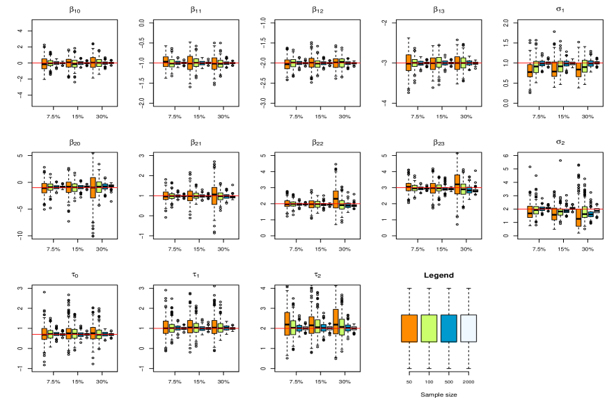
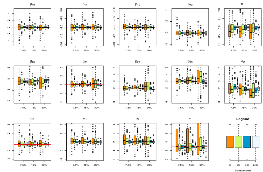
Figure 1: Boxplots of the ML parameter estimates for the MoE-N-CR model.

Figure 2: Boxplots of the ML parameter estimates for the MoE-T-CR model.

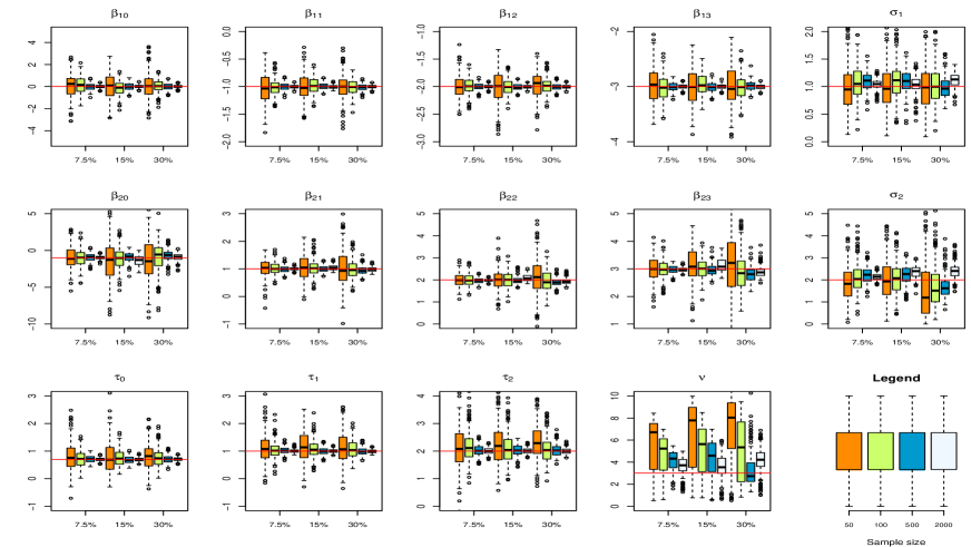
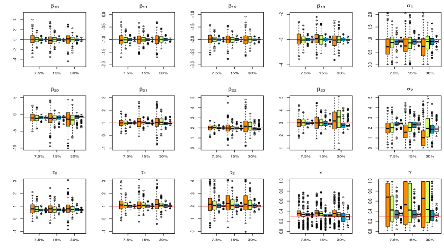
Figure 3: Boxplots of the ML parameter estimates for the MoE-SL-CR model.

Figure 4: Boxplots of the ML parameter estimates for the MoE-CN-CR model.

4.3 Model selection performance via information criteria

One of the challenges in the MoE models is to choose the optimal number of experts $G$. In dealing with this challenge, we conduct a simulation study to compare the ability of the proposed sub-models in the class of MoE-SMN-CR model to select the accurate $G$. We generate 100 sample of size $n=500$ from a three components (i.e. true $G$=3) MoE-SMN-CR model (5), where the mixing variable $U$ is followed by a generalized inverse Gaussian (GIG) distribution with parameters $\theta=(\kappa,\chi,\psi)$, denoted by the MoE-SGIG-CR model. Details of the GIG distribution and its new data-generating algorithm can be found in Hormann and Leydold (2013). It is assumed that the data is left-censored with levels 7.5%, 15% or 30%, $\bm{x}_{i}=\bm{r}_{i}=(1,x_{i1})^{\top}$ such that $x_{i1}\sim\mathcal{U}(-2,2)$, $\bm{\beta}_{1}=(-4,4)^{\top},$ $\bm{\beta}_{2}=(0,-2)^{\top}$, $\bm{\beta}_{3}=(0,4)^{\top}$, $\bm{\tau}_{1}=(0,13)^{\top}$, $\bm{\tau}_{2}=(2,9)^{\top}$, and $\theta_{1}=(-0.5,1,2)$, $\theta_{2}=(0.5,1,2)$, $\theta_{3}=(-0.5,2,1)$. Example of generated samples with and without censored cases are shown in Figure 5.

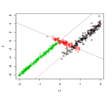
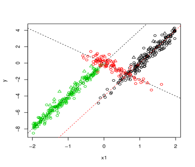
Figure 5: Simulated MoE-SGIG-CR data. Left-top panel: data without any censored observation. Right-top panel: data with 15% left-censored observations denoted by $\bigtriangleup$. Dash lines represent the true experts.

In this simulation study, we assume that the number of mixture components $G$ is unknown. We therefore fit the MoE-N-CR, MoE-T-CR, MoE-SL-CR and MoE-CN-CR models to the generated data in each replication, by assuming $G$ ranging form 1 to 5. The detailed numerical results including the average values of AIC and BIC together with the rate of correct model specification (RC; the mean of the number of replications in which the model with $G=3$ is outperformed) are reported in Table 1. Based on the RC measure, the MoE-T-CR, MoE-SL-CR and MoE-CN-CR models perform better than the MoE-N-CR model in identifying the number of components since the data are generated from a heavy-tailed distribution. Results depicted in Table 1 suggest that the BIC is more reliable than the AIC for model selection purpose and based on this measure the MoE-T-CR and MoE-SL-CR models outperform the other MoE models to fit to the data. In Figure 6, we plot the curve of the estimated experts to a dataset, with 15% censoring level, in which all models suggest $G=3$ based on the BIC. It could clearly be observed that the MoE-T-CR model fit the data better than the other models.

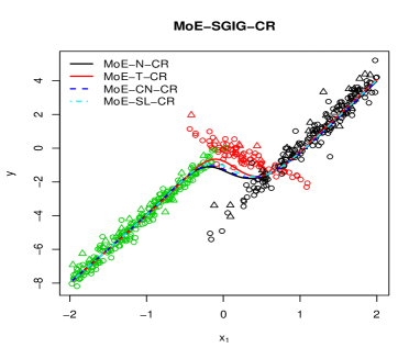
Figure 6: The estimated Experts curves of the special cases of the MoE-SMN-CR model for MoE-SGIG-CR simulated data with 15% left-censoring.

Table 1: The average of AIC and BIC, over 100 replications, by fitting special cases of the MoE-SMN-CR model to the generated data from the MoE-SGIG-CR model.

		$G=1$			$G=2$			$G=3$			$G=4$			$G=5$			RC
Model	Cens. Level	AIC	BIC		AIC	BIC		AIC	BIC		AIC	BIC		AIC	BIC		AIC	BIC
MoE-N-CR	$7.5\%$	1959.914	1972.558		1199.770	1233.487		937.685	$\bm{992.475}$		$\bm{918.283}$	994.146		929.686	1026.622		0.39	0.73
	$15\%$	1950.180	1962.310		1201.584	1231.051		954.333	$\bm{1007.388}$		939.155	1011.253		$\bm{931.957}$	1027.453		0.35	0.59
	$30\%$	1947.912	1960.556		1164.255	1197.972		886.857	$\bm{941.647}$		879.832	955.695		$\bm{867.216}$	964.152		0.35	0.78
MoE-T-CR	$7.5\%$	1944.642	1961.501		1031.442	1073.588		915.670	$\bm{983.104}$		$\bm{882.016}$	974.737		893.425	1011.434		0.58	0.83
	$15\%$	1936.854	1953.712		1037.712	1079.858		$\bm{892.430}$	$\bm{959.864}$		893.762	986.483		897.911	1015.920		0.59	0.80
	$30\%$	1924.194	1941.052		1018.596	1060.742		823.155	$\bm{890.588}$		814.159	906.880		$\bm{810.957}$	928.966		0.49	0.85
MoE-SL-CR	$7.5\%$	1945.130	1961.988		1048.648	1090.795		895.996	$\bm{963.430}$		$\bm{883.740}$	976.462		903.997	1022.006		0.61	0.84
	$15\%$	1937.009	1953.867		1076.567	1118.713		908.995	$\bm{976.428}$		$\bm{905.568}$	998.289		911.626	1029.635		0.62	0.78
	$30\%$	1924.250	1941.109		1044.162	1086.308		838.302	$\bm{905.735}$		$\bm{833.820}$	926.542		840.034	958.043		0.55	0.85
MoE-CN-CR	$7.5\%$	1946.769	1967.842		1094.680	1145.256		931.721	$\bm{1011.798}$		$\bm{910.684}$	1020.264		913.511	1052.592		0.58	0.77
	$15\%$	1938.737	1959.810		1136.442	1187.017		962.042	$\bm{1042.120}$		938.145	1047.725		$\bm{918.808}$	1057.890		0.40	0.70
	$30\%$	1927.552	1948.625		1089.598	1140.173		876.187	$\bm{956.264}$		871.465	981.045		$\bm{866.797}$	1005.879		0.54	0.90

4.4 Model performance in dealing with the highly peaked and thick-tailed data

In this simulation study, we simulate data with $n=100,500$ and 2000 observations from a three-component MoE-SMN-CR model via representation (3) under two generating scenarios of $U$. The first scenario (S1) is conducted by assuming $U^{-1}\sim\mathcal{E}(0.5)$, the exponential distribution with parameter $\lambda=0.5$, whereas the second one (S2) considers $U\sim\mathcal{BS}(\alpha,1)$, the Birnbaum-Saunders distribution (Birnbaum and Saunders, 1969) with parameter $\alpha$ and $\beta=1$. Bear in mind that the former scenario generates data from a Laplace distribution which is known as a highly peaked model and the later scenario provides a heavier tailed model than the normal distribution (Naderi et al., 2017b). The Laplace and BS censored MoE models, referred as the MoE-SLap-CR and MoE-SBS-CR, are not considered in this paper since their conditional expectations involved in the ECME algorithm are not exist.

In each replication of 200 trials, we generate data from the MoE-SLap-CR and MoE-SBS-CR models with three components, interval-censoring levels 7.5%, 15% or 30%, $\bm{x}_{i}=(1,x_{i1},x_{i2},x_{i3})^{\top}$ and $\bm{r}_{i}=(1,r_{i1})^{\top}$ , such that $x_{i1}\sim\mathcal{U}(1,5)$, $x_{i2}\sim U(0,1)$, $x_{i3}\sim U(-2,-1)$, and $r_{i1}\sim\mathcal{U}(-1,1)$, presumed parameter values given by $\bm{\theta}_{j}=(\bm{\beta}_{j},\sigma^{2}_{j},\bm{\nu}_{j}),~{}j=1,2,3$, $\bm{\beta}_{1}=(-2,-1,-2,-3)^{\top}$, $\bm{\beta}_{2}=(0.5,1,2,3)^{\top}$, $\bm{\beta}_{3}=(2,1,3,5)^{\top}$, $\sigma^{2}_{1}=1$, $\sigma^{2}_{2}=3$, $\sigma^{2}_{3}=5$, $\bm{\tau}_{1}=(2,10)^{\top}$, $\bm{\tau}_{2}=(0.7,10)^{\top}$ and $(\alpha_{1},\alpha_{2},\alpha_{3})=(3,1,2)$ for the MoE-SBS-CR model.

We compare the performance of the three-component MoE-N-CR, MoE-T-CR, MoE-SL-CR, and MoE-CN-CR models in terms of model selection indices (AIC and BIC) as well as clustering agreement measures (MCR, JCI, and ARI). Tables 2 and 3 present the average values of AIC, BIC, MCR, JCI and ARI over all 200 replications for the S1 and S2 scenarios of simulation, respectively. Results depicted in these tables reveal that the MoE-T-CR model outperforms the others in terms of AIC and BIC. Although the clustering performance of all models are very closed to each others, as expected from the MoE structurer, the MoE-T-CR and MoE-CN-CR models provide a slight improvement in the MCR, JCI and AIR over the MoE-N-CR and MoE-SL-CR models.

Table 2: The average of AIC, BIC, MCR and AIR, over 200 replications, by fitting special cases of the MoE-SMN-CR model to the generated data under S1 scenario.

Model $\rightarrow$		MoE-N-CR				MoE-T-CR				MoE-SL-CR				MoE-CN-CR
$n\;\downarrow$	Measure	$7.5\%$	$15\%$	$30\%$		$7.5\%$	$15\%$	$30\%$		$7.5\%$	$15\%$	$30\%$		$7.5\%$	$15\%$	$30\%$
	AIC	496.030	505.090	514.104		485.298	496.103	497.694		494.472	503.898	506.189		502.770	511.464	514.687
	BIC	545.528	554.588	563.602		542.612	553.417	555.008		551.786	561.212	563.503		567.901	576.594	579.817
100	MCR	0.165	0.192	0.222		0.175	0.185	0.225		0.165	0.178	0.216		0.158	0.175	0.213
	ARI	0.618	0.576	0.499		0.598	0.584	0.497		0.617	0.594	0.506		0.630	0.604	0.517
	JCI	0.632	0.602	0.551		0.619	0.608	0.548		0.630	0.616	0.553		0.641	0.621	0.560
	AIC	2370.929	2425.217	2618.009		2330.694	2369.694	2531.162		2338.787	2383.382	2554.371		2335.274	2378.907	2545.153
	BIC	2451.006	2505.295	2698.086		2423.415	2462.416	2623.884		2431.509	2476.104	2647.092		2440.640	2484.272	2650.518
500	MCR	0.162	0.167	0.214		0.153	0.163	0.201		0.154	0.158	0.186		0.155	0.157	0.187
	ARI	0.614	0.616	0.572		0.628	0.617	0.577		0.627	0.624	0.598		0.626	0.629	0.596
	JCI	0.630	0.634	0.597		0.642	0.635	0.601		0.642	0.641	0.616		0.639	0.642	0.612
	AIC	9397.490	9559.804	10548.390		9220.558	9278.635	10085.960		9255.169	9325.645	10221.340		9235.637	9310.615	10157.243
	BIC	9503.907	9666.221	10654.800		9343.778	9401.854	10209.180		9378.389	9448.865	10344.560		9370.060	9445.036	10291.67
2000	MCR	0.154	0.167	0.240		0.147	0.159	0.222		0.147	0.159	0.213		0.146	0.154	0.202
	ARI	0.634	0.614	0.521		0.644	0.621	0.530		0.645	0.623	0.541		0.647	0.623	.556
	JCI	0.645	.0632	0.559		0.654	.0637	0.564		0.656	0.641	0.571		0.656	0.644	0.580

Table 3: The average of AIC, BIC, MCR and AIR, over 200 replications, by fitting special cases of the MoE-SMN-CR model to the generated data under S2 scenario.

Model $\rightarrow$		MoE-N-CR				MoE-T-CR				MoE-SL-CR				MoE-CN-CR
$n\;\downarrow$	Measure	$7.5\%$	$15\%$	$30\%$		$7.5\%$	$15\%$	$30\%$		$7.5\%$	$15\%$	$30\%$		$7.5\%$	$15\%$	$30\%$
	AIC	522.443	542.212	556.691		498.602	514.384	533.806		508.967	525.134	544.353		502.185	521.979	538.774
	BIC	571.941	591.710	606.189		555.916	571.698	591.121		566.280	582.448	601.666		567.315	587.108	603.903
100	MCR	0.235	0.248	0.263		0.183	0.190	0.209		0.188	0.193	0.211		0.190	0.197	0.214
	ARI	0.498	0.472	0.448		0.589	0.571	0.541		0.584	0.563	0.539		0.581	0.557	0.535
	JCI	0.518	0.501	0.493		0.627	0.599	0.572		0.618	0.586	0.577		0.605	0.572	0.561
	AIC	2561.848	2564.510	2665.281		2432.404	2432.566	2503.707		2455.665	2464.471	2551.097		2490.907	2502.043	2799.294
	BIC	2641.925	2644.587	2745.358		2525.125	2525.288	2596.428		2548.386	2557.192	2643.818		2596.273	2607.408	2904.659
500	MCR	0.197	0.207	0.217		0.162	0.172	0.187		0.172	0.179	0.190		0.176	0.186	0.201
	ARI	0.588	0.553	0.533		0.636	0.602	0.574		0.624	0.585	0.563		0.618	0.574	0.545
	JCI	0.604	0.583	0.577		0.643	0.622	0.601		0.633	0.612	0.587		0.627	0.596	0.569
	AIC	10056.300	10424.278	10954.970		9576.709	9829.808	10326.340		9646.046	9956.371	10514.060		9654.003	9976.371	10527.060
	BIC	10162.717	10530.695	11061.380		9699.929	9953.028	10449.560		9769.266	10079.591	10637.280		9794.025	10110.791	10661.420
2000	MCR	0.214	0.223	0.255		0.171	0.174	0.216		0.189	0.178	0.218		0.171	0.181	0.219
	ARI	0.556	0.535	0.513		0.613	0.601	0.569		0.592	0.576	0.533		0.601	0.583	0.550
	JCI	0.578	0.560	0.553		0.644	0.619	0.598		0.607	0.596	0.563		0.626	0.603	0.569

4.5 Sensitivity analysis in presence of outliers

The last simulation study aims at investigating the robustness on estimating MoE-SMN-CR models in which some outliers are introduced into the simulated data. Each of the three models MoE-SLap-CR, MoE-SBS-CR and MoE-SGIG-CR is considered for data generation. Following Nguyen and McLachlan (2016), we setup $\bm{x}_{i}=\bm{r}_{i}=(1,x_{i1})^{\top}$ where $x_{i1}$ is generated from $\mathcal{U}(-1,1)$, $\bm{\beta}_{1}=(0,1)^{\top},$ $\bm{\beta}_{2}=(0,-1)^{\top}$, $\sigma^{2}_{1}=\sigma^{2}_{2}=0.01$ $\bm{\tau}_{1}=(0,10)^{\top}$, $\theta_{1}=(-0.5,1,0.2)$, $\theta_{2}=(0.5,1,0.2)$ for the MoE-SGIG-CR model and $(\alpha_{1},\alpha_{2})=(0.5,1)$ for the MoE-SBS-CR model. We assume left-censoring scheme with levels 7.5% or 30% and sample size 500. We also add class of outliers with varying probability $c$ ranging from 0% to 6% by simulating the predictor $x$ from $\mathcal{U}(-1,1)$ and the response $y$ is set the value -2 (Nguyen and McLachlan, 2016). An example of simulated samples with left-censoring level 7.5% form the MoE-SLap-CR, MoE-SBS-CR and MoE-SGIG-CR models and containing 6% outliers is shown in Figure 7. In each trial of 500 replications, the MoE-N-CR, MoE-T-CR, MoE-CN-CR, and MoE-SL-CR models are fitted to the generated data. Figure 8 shows an example fitted MoE curves to the data generated from the MoE-SLap-CR, MoE-SBS-CR and MoE-SGIG-CR models. It can obviously be seen that the heavy-tailed models provide better fit and platforms for describing the data than the MoE-N-CR model.

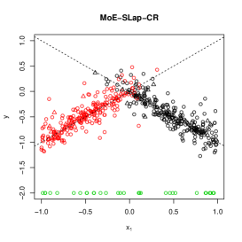
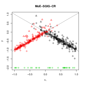
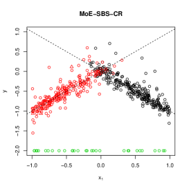
Figure 7: Scatterplots of the simulated data with 7.5% left-censoring ($\triangle$) generated from the MoE-SLap-CR, MoE-SBS-CR and MoE-SGIG-CR models and containing 6% outliers (green $\circ$). Dash lines represent the true experts.

Table 4: Simulation results for assessing the robustness of the proposed MoE model to outliers under various censoring levels and outliers percentages.

	Cens. Level $\rightarrow$	7.5%					30%
True model	Fitted model	0%	2%	4%	6%		0%	2%	4%	6%
	MoE-N-CR	0.0347	0.0948	0.1418	0.1897		0.1029	0.1626	0.2357	0.2776
MoE-SGIG-CR	MoE-T-CR	0.0297	0.0855	0.1195	0.1623		0.0698	0.1375	0.1857	0.2068
	MoE-CN-CR	0.0334	0.0865	0.1232	0.1692		0.0928	0.1379	0.2013	0.2481
	MoE-SL-CR	0.0300	0.0856	0.1201	0.1642		0.0733	0.1392	0.1891	0.2161
	MoE-N-CR	0.0385	0.0979	0.1436	0.1936		0.1061	0.1657	0.2338	0.2788
MoE-SBS-CR	MoE-T-CR	0.0342	0.0885	0.1226	0.1654		0.0735	0.1416	0.1918	0.2292
	MoE-CN-CR	0.0375	0.0897	0.1260	0.1729		0.0981	0.1427	0.2076	0.2507
	MoE-SL-CR	0.0344	0.0889	0.1230	0.1662		0.0789	0.1437	0.1932	0.2284
	MoE-N-CR	0.0451	0.1050	0.1512	0.1978		0.1142	0.1772	0.2401	0.2892
MoE-SLap-CR	MoE-T-CR	0.0406	0.0950	0.1287	0.1712		0.0827	0.1519	0.1979	0.2289
	MoE-CN-CR	0.0437	0.0963	0.1329	0.1779		0.1032	0.1539	0.2165	0.2562
	MoE-SL-CR	0.0407	0.0953	0.1290	0.1719		0.0886	0.1548	0.2010	0.2394

To assess the impact of the outliers on the parameter estimates and on the quality of the results, we calculate, in each 500 replications, the mean square error between the true regression mean function and the estimated one, defined as

$$\text{MSE}=\frac{1}{500}\sum_{i=1}^{500}\Big{(}E_{\hat{\bm{\Theta}}}(\bm{x}_{i},\bm{r}_{i})-E_{\bm{\Theta}_{true}}(\bm{x}_{i},\bm{r}_{i})\Big{)}^{2},$$

where $E_{\bm{\Theta}}(\bm{x}_{i},\bm{r}_{i})=\sum_{j=1}^{G}\pi_{j}(\bm{r}_{i};\bm{\tau})\bm{x}_{i}^{\top}\bm{\beta}_{j}$ evaluated at the true and estimated parameters. Table 4 shows, for each of the four MoE models, the average of MSE for an increasing percentage of outliers and censoring in the data. First, one can see that the MSE tends towered zero as the level of censoring and outliers approach zeros for all cases of the MoE-SMN-CR model. Since the three considered scenarios generate fat-tailed data, it can be observed that without outliers (c = 0%) the error of the MoE-N-CR model is greater than those of the other MoE models, reflecting its lack of robustness. Upon inspection of Table 4, one can conclude that by adding outliers to the data, the MoE-T-CR (and the MoE-SL-CR in the second order) model clearly outperforms others for all situations. It highlights that the MoE-T-CR model is much more robust to outliers under these data generating scenarios.

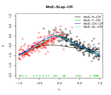
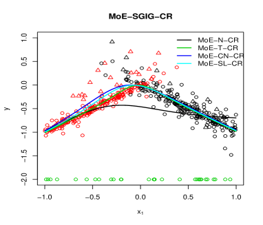
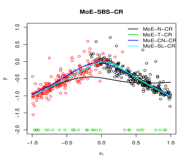
Figure 8: Scatter plots of the artificial data with 7.5% left-censoring ($\triangle$) generated from the MoE-SLap-CR, MoE-SBS-CR and MoE-SGIG-CR models and containing 6% outliers (green $\circ$).

5 Real data analysis

This section considers the wage rates of 753 married women dataset, previously analyzed by Mroz (1987); Caudill (2012); Karlsson and Laitila (2014), for illustrative purposes of the developed novel MoE-SMN-CR model. This dataset contains 753 observed wage rates (hours of working outside the home) of married white women between the ages of 30 and 60 in 1975, of whom 325 have zero hours working. Recently, Zeller et al. (2018) reanalyzed the wage-rates dataset in order to illustrate the performance of the FM of censored linear regression models based on the SMN class of distributions which is made available in the $\mathtt{R}$ package “CensMixReg”. Hereafter, we will denote the FM of censored linear regression models based on the normal, Student-$t$, slash and contaminated-normal distributions (Zeller et al., 2018), respectively by FM-N-CR, FM-T-CR, FM-SL-CR and FM-CN-CR. By considering the wife’s annual work hours outside home scaled by 1000 as the response variable ($y$) which has 43.16% level of left-censoring, and the explanatory variables including ($x_{1}$) the wife’s education in years, ($x_{2}$) the wife’s age, ($x_{3}$) the wife’s previous labor market experience and ($x_{4}$) the wife’s previous labor market experience squared, Caudill (2012); Karlsson and Laitila (2014) and Zeller et al. (2018) concluded that a mixture of two components linear regression censored model provides an appropriate platform for analyzing this dataset. Figure 9 shows the histograms of $y$ overlaid with the estimated kernel density curve. The bimodality of the data and the suitability of the two-component mixture model to fit the data can be observed. It could be mentioned from the histogram that this is a heavily right-tailed data.

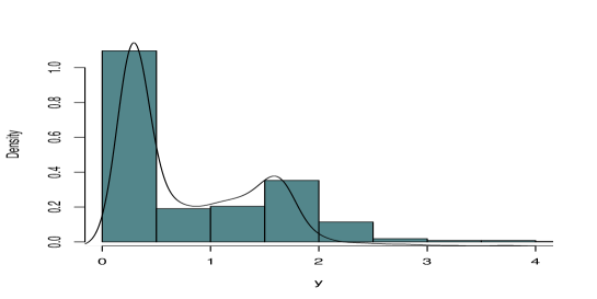
Figure 9: The histogram of the response variable $y$ overlaid with its Kernel density estimate.

The FM modeling allows clustering of the data in terms of the estimated (posterior) probability, $\hat{z}_{ij}$, that a single point belongs to a given group. Although the previous works on the wage-rates dataset focused on the aforementioned explanatory variables and showed that only these variables have significant effects on $y$, there are eleven measures that could provide more information in investigating the complex relationship of random phenomena under study. One of those variable that we will use for clustering purposes is the living status, labeled as “city”, that takes 1 for living in the city and 0 for otherwise. Assuming “city” as the group indicator, one can obtain the posterior probability $\hat{z}_{ij}$ and can therefore compute the clustering criteria MCR, RI, ARI and JCI of the FM regression models proposed by Zeller et al. (2018). In this regard, the posterior probabilities of the two-component FM-N-CR, FM-T-CR, FM-SL-CR and FM-CN-CR models are computed by fitting them to the considered data. It is observed that all of the models proposed by Zeller et al. (2018) assign data points to one group.

As the advantages of the MoE model, it is possible for the investigator to choose some covariates for the gating function. In analyzing wage-rates data, we consider $\bm{x}=(1,x_{1},x_{2},x_{3},x_{4})^{\top}$ and $\bm{r}=(1,r_{1},r_{2},x_{2})^{\top}$ for gating function, where ($r_{1}$) is the unemployment rate in county of residence and ($r_{2}$) is the number of kids less than 6 years old. We note that the covariates of the gating function can be the same as $\bm{x}$, however by considering various combinations of the available explanatory variables, we observe that these three variables provide a better clustering performance. An interesting open issue for future work could be the variable selection problem for both $\bm{x}$ and $\bm{r}$ in the MoE models.

By fitting the MoE-N-CR, MoE-T-CR, MoE-SL-CR, and MoE-CN-CR models to these data for $G=1,\ldots,4$, the two-component MoE model has been selected based on the BIC. It should be noted that our results are not directly comparable with those obtained by Karlsson and Laitila (2014) since they imposed some restrictions on $\bm{\beta}$ for estimation. Moreover, it is clear that adding more variables to the model will definitely affect on the likelihood. We therefore can not compare the results of model selection criteria, the AIC and BIC, with those reported by Zeller et al. (2018). Table 5 shows the ML results obtained by fitting the four considered models. The information-based approach for approximating standard error (SE) of parameter estimates are given in C. We found that the estimated gating parameters are moderately significant, revealing that the considered covariates $\bm{r}$ have an effect on the analysis. Results based on AIC and BIC indicate that the MoE-T-CR and MoE-SL-CR models provides an improved fit of the data over the other models. Moreover, by comparing the clustering criteria in Tables 5, it turns out that the MoE-SL-CR models yields quite better classification.

Table 5: ML estimates with corresponding approximate standard errors(SE) together with their AIC, BIC, and clustering performance measures.

		MoE-N-CR			MoE-T-CR			MoE-SL-CR			MoE-CN-CR
Parameter $\downarrow$		Estimates	SE		Estimates	SE		Estimates	SE		Estimates	SE
$\beta_{10}$		5.5476	0.6362		5.5438	0.6573		5.6223	0.7524		5.4714	0.9077
$\beta_{11}$		-0.0554	0.0268		-0.0627	0.0027		-0.0658	0.0287		-0.0607	0.0227
$\beta_{12}$		-0.1272	0.0130		-0.1256	0.0014		-0.1227	0.0167		-0.1212	0.0212
$\beta_{13}$		0.0653	0.0355		0.0822	0.0050		0.0371	0.0063		0.0485	0.0114
$\beta_{14}$		0.0004	0.0002		-0.0003	0.0001		0.0013	0.0029		0.0009	0.0007
$\beta_{20}$		1.5064	0.2850		0.7306	0.0675		1.3579	0.4638		1.3405	0.2478
$\beta_{21}$		0.0165	0.0025		0.0109	0.0025		0.0259	0.0051		0.0212	0.0028
$\beta_{22}$		-0.0592	0.0125		-0.0410	0.0013		-0.0578	0.0109		-0.0560	0.0098
$\beta_{23}$		0.2418	0.0205		0.2424	0.0018		0.2426	0.0207		0.2404	0.0128
$\beta_{24}$		-0.0047	0.0006		-0.0049	0.0001		-0.0048	0.0007		-0.0047	0.0021
$\sigma^{2}_{1}$		0.5001	0.0682		0.4365	0.0066		0.3773	0.0836		0.4173	0.1109
$\sigma^{2}_{2}$		0.7130	0.0568		0.4661	0.0043		0.3120	0.0367		0.4214	0.1291
$\nu_{1}$		–	–		9.3049	–		9.0866	–		0.0342	–
$\nu_{2}$		–	–		6.2745	–		1.8225	–		0.1577	–
$\gamma$		–	–		–	–		–	–		0.2643	–
$\gamma$		–	–		–	–		–	–		0.2237	–
$\tau_{0}$		26.7338	5.6234		48.3470	6.3394		14.4513	3.9352		17.4136	4.6459
$\tau_{1}$		0.2519	0.1023		0.3414	0.2210		0.1845	0.0138		0.1999	0.0851
$\tau_{2}$		4.1959	1.2368		6.9057	1.7441		0.8211	0.1362		0.7284	0.1246
$\tau_{3}$		-0.7383	0.2304		-1.2943	0.3588		-0.4177	0.1394		-0.4912	0.1537
AIC		1234.5830			1219.2230			1219.2830			1224.094
BIC		1308.5680			1302.4570			1302.5160			1316.575
RI		0.5123			0.5214			0.5323			0.5118
JCI		0.3676			0.3847			0.4029			0.3713

6 Conclusions and discussions

This paper proposed a new robust mixture of linear experts model for the censored data based on the scale-mixture of normal class of distributions. This MoE-SMN-CR model extended the classical MoE model which has been demonstrated to solve the two challenges to deal with heavy-tail distributed data and outliers as well as censored data. The newly proposed MoE-SMN-CR model is very extensive which extends the classical MoE model and includes FM regression and FM regression for censored data proposed by Zeller et al. (2018) as special cases. The use of covariates in the gating function is an advantage of the MoE models which might result in better classification of the data. Utilizing the embedded hierarchical structure of the SMN class of distributions, we developed an innovative EM-type algorithm to obtain ML parameter estimates computationally. We implemented this model in $\mathtt{R}$ and the computing program can be obtained from the authors upon request.

Four Monte-Carlo simulation studies were conducted to investigate the performance of the model in applications both for non-linear regression and prediction and for model-based clustering. Results of simulation studies confirmed that the proposed MoE-SMN-CR model can provide evidence of the robustness to the outliers and atypical observations. Finally, a real-world data analysis demonstrated the applicability and benefit of the proposed approach for practical applications.

As discussed in Section 5, an interesting future direction of the current work is the variable selection for both parts of the regression and gating function. The utility of our current approach can be further extended to the multiple regression on multivariate data rather than simple regression on univariate data, which we are actively exploring. Another possible extension of the work herein is to consider a full Bayesian approach as a basis of inference and prediction (Peng et al., 1996; Zens, 2019).

Appendix A Conditional expectations of the special cases of the SMN distributions

Uncensored observations: For the uncensored data $y_{i}$, we have $\rho_{i}=0$. Therefore, the only necessary conditional expectation $\hat{u}_{ij}^{(k)}=E(U_{ij}|Y=y_{i},\hat{\bm{\theta}}_{j}^{(k)})$ for the considered models can be computed as follows.

• If $Y\sim\mathcal{N}\big{(}\bm{x}_{i}^{\top}\hat{\bm{\beta}}_{j}^{(k)},\hat{\sigma}_{j}^{2(k)}\big{)}$, in this case, $U=1$ with probability one, and so $\hat{u}_{ij}^{(k)}=1$

• If $Y\sim\mathcal{T}\big{(}\bm{x}_{i}^{\top}\hat{\bm{\beta}}_{j}^{(k)},\hat{\sigma}_{j}^{2(k)},\hat{\nu}_{j}^{(k)}\big{)}$, We have

  $$\hat{u}_{ij}^{(k)}=\frac{\hat{\nu}_{j}^{(k)}+1}{\hat{\nu}_{j}^{(k)}+\delta\Big{(}y_{i},\bm{x}_{i}^{\top}\hat{\bm{\beta}}_{j}^{(k)},\hat{\sigma}_{j}^{(k)}\Big{)}},$$

  where $\delta(y,\mu,\sigma)=\Big{(}(y-\mu)/\sigma\Big{)}^{2}$.

• If $Y\sim\mathcal{SL}\big{(}\bm{x}_{i}^{\top}\hat{\bm{\beta}}_{j}^{(k)},\hat{\sigma}_{j}^{2(k)},\hat{\nu}_{j}^{(k)}\big{)}$, We have

  $$\hat{u}_{ij}^{(k)}=2\left(\delta\Big{(}y_{i},\bm{x}_{i}^{\top}\hat{\bm{\beta}}_{j}^{(k)},\hat{\sigma}_{j}^{(k)}\Big{)}\right)^{-1}\frac{\Gamma\left(\hat{\nu}_{j}^{(k)}+1.5,\;0.5\delta\Big{(}y_{i},x_{i}^{\top}\hat{\bm{\beta}}_{j}^{(k)},\hat{\sigma}_{j}^{(k)}\Big{)}\right)}{\Gamma\left(\hat{\nu}_{j}^{(k)}+0.5,\;0.5\delta\Big{(}y_{i},\bm{x}_{i}^{\top}\hat{\bm{\beta}}_{j}^{(k)},\hat{\sigma}_{j}^{(k)}\Big{)}\right)}.$$

• If $Y\sim\mathcal{CN}\big{(}\bm{x}_{i}^{\top}\hat{\bm{\beta}}_{j}^{(k)},\hat{\sigma}_{j}^{2(k)},\hat{\nu}_{j}^{(k)},\hat{\gamma}_{j}^{(k)}\big{)}$, We have

  $$\hat{u}_{ij}^{(k)}=\frac{1-\hat{\nu}_{j}^{(k)}+\hat{\nu}_{j}^{(k)}(\hat{\gamma}_{j}^{(k)})^{1.5}\exp\Big{\{}0.5(1-\hat{\gamma}_{j}^{(k)})\delta\Big{(}y_{i},\bm{x}_{i}^{\top}\hat{\bm{\beta}}_{j}^{(k)},\hat{\sigma}_{j}^{(k)}\Big{)}\Big{\}}}{1-\hat{\nu}_{j}^{(k)}+\hat{\nu}_{j}^{(k)}(\hat{\gamma}_{j}^{(k)})^{0.5}\exp\Big{\{}0.5(1-\hat{\gamma}_{j}^{(k)})\delta\Big{(}y_{i},\bm{x}_{i}^{\top}\hat{\bm{\beta}}_{j}^{(k)},\hat{\sigma}_{j}^{(k)}\Big{)}\Big{\}}}.$$

Censored cases: In the censored cases, we have $\rho_{i}=1$. For the sake of notation, let

$$T_{ij}^{(k)}=\dfrac{Y_{i}-\bm{x}_{i}^{\top}\hat{\bm{\beta}}_{j}^{(k)}}{\hat{\sigma}_{j}^{(k)}}\sim\text{SMN}(0,1,\hat{\bm{\nu}}_{j}^{(k)}),\qquad\hat{t}_{ij1}^{(k)}=\frac{c_{i1}-\bm{x}_{i}^{\top}\hat{\bm{\beta}}_{j}^{(k)}}{\hat{\sigma}_{j}^{(k)}},\qquad\hat{t}_{ij2}^{(k)}=\frac{c_{i2}-\bm{x}_{i}^{\top}\hat{\bm{\beta}}_{j}^{(k)}}{\hat{\sigma}_{j}^{(k)}}.$$

Therefore, the necessary conditional expectations $\hat{u}_{ij}^{(k)}=E(U_{ij}|c_{i1}\leq Y_{i}\leq c_{i2},\hat{\bm{\theta}}_{j}^{(k)})$, $\widehat{uy}_{ij}^{(k)}=E(U_{i}Y_{i}|c_{i1}\leq Y_{i}\leq c_{i2},\hat{\bm{\theta}}_{j}^{(k)})$, and $\widehat{uy^{2}}_{ij}^{(k)}=E(U_{i}Y_{i}^{2}|c_{i1}\leq Y_{i}\leq c_{i2},\hat{\bm{\theta}}_{j}^{(k)})$ for the considered models can be computed as follows.

$$\hat{u}_{ij}^{(k)}=E\left(U_{ij}|\hat{t}_{ij1}^{(k)}\leq T_{ij}^{(k)}\leq\hat{t}_{ij2}^{(k)},\hat{\bm{\theta}}_{j}^{(k)}\right)=\frac{E_{\Phi}\left(1,\hat{t}_{ij2}^{(k)}\right)-E_{\Phi}\left(1,\hat{t}_{ij1}^{(k)}\right)}{F_{SMN}\left(\hat{t}_{ij2}^{(k)};\hat{\bm{\nu}}_{j}^{(k)}\right)-F_{SMN}\left(\hat{t}_{ij1}^{(k)};\hat{\bm{\nu}}_{j}^{(k)}\right)},$$

$$\widehat{uy}_{ij}^{(k)}= \left(x_{i}^{\top}\hat{\bm{\beta}}_{j}^{(k)}\right)\widehat{u}_{ij}^{(k)}+\hat{\sigma}_{j}^{(k)}E\left(U_{ij}T_{ij}\Big{|}\hat{t}_{ij1}^{(k)}\leq T_{ij}^{(k)}\leq\hat{t}_{ij2}^{(k)},\hat{\bm{\theta}}_{j}^{(k)}\right)$$

$$= \left(x_{i}^{\top}\hat{\bm{\beta}}_{j}^{(k)}\right)\left\{\frac{E_{\Phi}\left(1,\hat{t}_{ij2}^{(k)}\right)-E_{\Phi}\left(1,\hat{t}_{ij1}^{(k)}\right)}{F_{SMN}\left(\hat{t}_{ij2}^{(k)};\hat{\bm{\nu}}_{j}^{(k)}\right)-F_{SMN}\left(\hat{t}_{ij1}^{(k)};\hat{\bm{\nu}}_{j}^{(k)}\right)}\right\}+\hat{\sigma}_{j}^{(k)}\left\{\frac{E_{\phi}\left(0.5,\hat{t}_{ij1}^{(k)}\right)-E_{\phi}\left(0.5,\hat{t}_{ij2}^{(k)}\right)}{F_{SMN}\left(\hat{t}_{ij2}^{(k)};\hat{\bm{\nu}}_{j}^{(k)}\right)-F_{SMN}\left(\hat{t}_{ij1}^{(k)};\hat{\bm{\nu}}_{j}^{(k)}\right)}\right\},$$

$$\widehat{uy^{2}}_{ij}^{(k)}= \left(x_{i}^{\top}\hat{\bm{\beta_{j}}}^{(k)}\right)^{2}\widehat{u}_{ij}^{(k)}+2\left(x_{i}^{\top}\hat{\bm{\beta_{j}}}^{(k)}\right)\hat{\sigma}_{j}^{(k)}\widehat{uy}_{ij}^{(k)}+\hat{\sigma}_{j}^{2(k)}E\left(U_{ij}T_{ij}^{2}\Big{|}\hat{t}_{ij1}^{(k)}\leq T_{ij}^{(k)}\leq\hat{t}_{ij2}^{(k)},\hat{\bm{\theta}}_{j}^{(k)}\right),$$

$$= \left(x_{i}^{\top}\hat{\bm{\beta_{j}}}^{(k)}\right)^{2}\widehat{u}_{ij}^{(k)}+2\left(x_{i}^{\top}\hat{\bm{\beta_{j}}}^{(k)}\right)\hat{\sigma}_{j}^{(k)}\widehat{uy}_{ij}^{(k)}+\frac{\hat{\sigma}_{j}^{2(k)}}{F_{SMN}\left(\hat{t}_{ij2}^{(k)};\hat{\bm{\nu}}_{j}^{(k)}\right)-F_{SMN}\left(\hat{t}_{ij1}^{(k)};\hat{\bm{\nu}}_{j}^{(k)}\right)}$$

$$\qquad\left(E_{\Phi}\left(0,\hat{t}_{ij2}^{(k)}\right)-E_{\Phi}\left(0,\hat{t}_{ij1}^{(k)}\right)+\left(\hat{t}_{ij1}^{(k)}\right)E_{\phi}\left(0.5,\hat{t}_{ij1}^{(k)}\right)-\left(\hat{t}_{ij2}^{(k)}\right)E_{\phi}\left(0.5,\hat{t}_{ij2}^{(k)}\right)\right),$$

where

$$E_{\phi}(r,h)=E\left(U^{r}\phi\big{(}h\sqrt{U}\big{)}\right)\quad\text{and}\quad E_{\Phi}(r,h)=E\left(U^{r}\Phi\big{(}h\sqrt{U}\big{)}\right).$$

In the following, the closed forms of $E_{\phi}(r,h)$ and $E_{\Phi}(r,h)$ for the special cases of SMN class of distributions are presented.

• For the normal distribution, we have

  $$E_{\phi}(r,h)=\phi(h)\quad\text{and}\quad E_{\Phi}(r,h)=\Phi(h).$$

• In the case of Student-$t$ distribution, we have

  $$E_{\phi}(r,h) =\frac{\Gamma\left(\dfrac{\hat{\nu}_{j}^{(k)}+2r}{2}\right)}{\sqrt{2\pi}\Gamma(\hat{\nu}_{j}^{(k)}/2)}\left(\frac{\hat{\nu}_{j}^{(k)}}{2}\right)^{\dfrac{\hat{\nu}_{j}^{(k)}}{2}}\left(\frac{2}{h^{2}+\hat{\nu}_{j}^{(k)}}\right)^{\dfrac{\hat{\nu}_{j}^{(k)}+2r}{2}},$$

  $$E_{\Phi}(r,h) =\Gamma\left(\frac{\hat{\nu}_{j}^{(k)}+2r}{2}\right)\left(\frac{2}{\hat{\nu}_{j}^{(k)}}\right)^{r}F_{PVII}\left(h;\hat{\nu}_{j}^{(k)}+2r,\hat{\nu}_{j}^{(k)}\right)\Big{/}\Gamma(\frac{\hat{\nu}_{j}^{(k)}}{2}).$$

  where $F_{PVII}(\cdot;\nu,\delta)$ denotes the cdf of Pearson type $VII$ distribution.

• For the slash model, we have

  $$E_{\phi}(r,h)=\frac{\hat{\nu}_{j}^{(k)}}{\sqrt{2\pi}}\left(\frac{2}{h^{2}}\right)^{\hat{\nu}_{j}^{(k)}+r}\Gamma(\hat{\nu}_{j}^{(k)}+r,\frac{h^{2}}{2})\quad\text{and}\quad E_{\Phi}(r,h)=\frac{\hat{\nu}_{j}^{(k)}}{\hat{\nu}_{j}^{(k)}+r}F_{SL}\left(h;\hat{\nu}_{j}^{(k)}+r\right).$$

• For the contaminated-normal distribution, we have

  $$E_{\phi}(r,h) =\left(\hat{\gamma}_{j}^{(k)}\right)^{r}\hat{\nu}_{j}^{(k)}\phi\left(h\sqrt{\hat{\gamma_{j}}^{(k)}}\right)+\left(1-\hat{\nu}_{j}^{(k)}\right)\phi(h),$$

  $$E_{\Phi}(r,h) =\left(\hat{\gamma_{j}}^{(k)}\right)^{r}F_{CN}\left(h;\hat{\nu}_{j}^{(k)},\hat{\gamma}_{j}^{(k)}\right)+\left(1-\left(\hat{\gamma}_{j}^{(k)}\right)^{r}\right)\left(1-\hat{\nu}_{j}^{(k)}\right)\Phi(h).$$

Appendix B The hazard function plot of the normal distribution

Figure 10: The normal hazard function plots computed based on three ways in $\mathtt{R}$.

Appendix C Standard error estimates

For estimating the standard error of the ML estimators, we follow Meilijson (1989) to exploit an information-based method for calculating the asymptotic covariance matrix of the ML estimates. Let $\ell_{ci}$ be the complete-data log-likelihood contributed from the $i$th observation. i.e.

$$\ell_{ci}=\ell_{c}(\bm{\Theta}|\bm{w}_{i}^{\top},\bm{\rho}_{i}^{\top},\bm{y}_{i}^{\top},\bm{u}_{i}^{\top},\bm{Z}_{i}^{\top})=\sum_{j=1}^{G}Z_{ij}\left\{\log\pi_{j}(\bm{r}_{i};\bm{\tau})-\frac{1}{2}\log\sigma_{j}^{2}-\frac{u_{i}}{2\sigma_{j}^{2}}(y_{i}-\bm{x}_{i}^{\top}\bm{\beta}_{j})^{2}+\log h(u_{i};\bm{\nu}_{j})\right\},$$

Then, the Fisher information matrix can be approximated by

$$I_{o}(\hat{\Theta}|\bm{y})=\sum_{i=1}^{n}\hat{\bm{s}}_{i}\hat{\bm{s}}_{i}^{\top},$$

where $\hat{s}_{i}=E\Big{(}\dfrac{\partial\ell_{ci}}{\partial\bm{\Theta}}\;\Big{|}\;y_{i},\hat{\bm{\Theta}}\Big{)}$ is the individual score vector corresponding to the $i$th observation. The elements of individual score vector $(\hat{s}_{i,\bm{\tau}_{1}}^{\top},\ldots,\hat{s}_{i,\bm{\tau}_{G-1}}^{\top}\hat{s}_{i,\bm{\beta}_{1}}^{\top},\ldots,\hat{s}_{i,\bm{\beta}_{G}}^{\top},\hat{s}_{i,\sigma_{1}^{2}},\ldots,\hat{s}_{i,\sigma_{G}^{2}})$ have the explicit forms as

$$\hat{s}_{i,\bm{\tau}_{j}} =E\Big{(}\dfrac{\partial\ell_{ci}}{\partial\bm{\tau}_{j}}\;\Big{|}\;y_{i},\hat{\bm{\Theta}}\Big{)}=\left(\hat{z}_{ij}-\pi_{j}(\bm{r}_{i};\hat{\bm{\tau}})\right)\bm{r}_{i},\qquad\hat{s}_{i,\bm{\beta}_{j}}=E\Big{(}\dfrac{\partial\ell_{ci}}{\partial\bm{\beta}_{j}}\;\Big{|}\;y_{i},\hat{\bm{\Theta}}\Big{)}=\frac{\hat{z}_{ij}}{\hat{\sigma}_{j}^{2}}\left(\widehat{uy}_{ij}\bm{x}_{i}-\hat{u}_{ij}\bm{x}_{i}^{\top}\hat{\bm{\beta}}_{j}\bm{x}_{i}\right),$$

$$\hat{s}_{i,\sigma_{j}^{2}} =E\Big{(}\dfrac{\partial\ell_{ci}}{\partial\sigma_{j}^{2}}\;\Big{|}\;y_{i},\hat{\bm{\Theta}}\Big{)}=-\frac{\hat{z}_{ij}}{2\hat{\sigma}_{j}^{4}}\left(\hat{\sigma}_{j}^{2}-\widehat{uy^{2}}_{ij}-\hat{u}_{ij}(\bm{x}_{i}^{\top}\hat{\bm{\beta}}_{j})^{2}+2\widehat{uy}_{ij}\bm{x}_{i}^{\top}\hat{\bm{\beta}}_{j}\right).$$

As a result, the variance of the ML estimates can be consistently estimated from the diagonal of the inverse of $I_{o}(\hat{\Theta}|\bm{y})$ under some regularity conditions. We note that the standard error of $\hat{\nu}$ critically depends on the calculation of $E\big{(}\log(U_{i})|y_{i},\hat{\bm{\Theta}}\big{)}$ which is a computational challenge. It could be mentioned that inverse of the $I_{o}(\hat{\Theta}|\bm{y})$ is not always available. One can refer to Yu et al. (2021) to find an innovative interpolation procedure based on the cubic spline interpolation to directly estimate the asymptotic variance-covariance matrix of the ML estimates obtained by the EM algorithm.

References

- Akaike (1974) Akaike, H., 1974. A new look at the statistical model identification, in: Selected Papers of Hirotugu Akaike. Springer, pp. 215–222.
- Birnbaum and Saunders (1969) Birnbaum, Z.W., Saunders, S.C., 1969. A new family of life distributions. Journal of applied probability 6, 319–327.
- Caudill (2012) Caudill, S.B., 2012. A partially adaptive estimator for the censored regression model based on a mixture of normal distributions. Statistical Methods & Applications 21, 121–137.
- Chamroukhi (2016) Chamroukhi, F., 2016. Robust mixture of experts modeling using the t distribution. Neural Networks 79, 20–36.
- Chamroukhi (2017) Chamroukhi, F., 2017. Skew mixture of experts. Neurocomputing 266, 390–408.
- Cuesta-Albertos et al. (1997) Cuesta-Albertos, J.A., Gordaliza, A., Matrá n, C., et al., 1997. Trimmed -means: An attempt to robustify quantizers. The Annals of Statistics 25, 553–576.
- Dempster et al. (1977) Dempster, A.P., Laird, N.M., Rubin, D.B., 1977. Maximum likelihood from incomplete data via the EM algorithm. Journal of the Royal Statistical Society: Series B (Methodological) 39, 1–22.
- Feigelson and Babu (2012) Feigelson, E.D., Babu, G.J., 2012. Modern statistical methods for astronomy: with R applications. Cambridge University Press.
- Garay et al. (2017) Garay, A.M., Lachos, V.H., Bolfarine, H., Cabral, C.R., 2017. Linear censored regression models with scale mixtures of normal distributions. Statistical Papers 58, 247–278.
- Garay et al. (2016) Garay, A.M., Lachos, V.H., Lin, T.I., 2016. Nonlinear censored regression models with heavy-tailed distributions. Stat Interface 9, 281–293.
- Gomez et al. (2009) Gomez, G., Calle, M.L., Oller, R., Langohr, K., 2009. Tutorial on methods for interval-censored data and their implementation in R. Statistical Modelling 9, 259–297.
- Hartigan and Wong (1979) Hartigan, J.A., Wong, M.A., 1979. Algorithm as 136: A -means clustering algorithm. Journal of the Royal Statistical Society. Series C (Applied Statistics) 28, 100–108.
- Hu et al. (2017) Hu, H., Yao, W., Wu, Y., 2017. The robust EM-type algorithms for log-concave mixtures of regression models. Computational Statistics & Data Analysis 111, 14–26.
- Hubert (1985) Hubert, L., Arabie, P., 1985. Comparing partitions. Journal of classification 2, 193–218.
- Hormann and Leydold (2013) Hormann , W., Leydold, J., 2013. Generating generalized inverse Gaussian random variates. Statistics and Computing 24, 547–557.
- Jacobs et al. (1991) Jacobs, R.A., Jordan, M.I., Nowlan, S.J., Hinton, G.E., et al., 1991. Adaptive mixtures of local experts. Neural computation 3, 79–87.
- Karlsson and Laitila (2014) Karlsson, M., Laitila, T., 2014. Finite mixture modeling of censored regression models. Statistical papers 55, 627–642.
- Kaufman and Rousseeuw (1990) Kaufman, L., Rousseeuw, P.J., 1990. Finding groups in data. John Wiley & Sons, Hoboken, New Jersey.
- Lachos et al. (2019) Lachos, V.H., Cabral, C.R., Prates, M.O., Dey, D.K., 2019. Flexible regression modeling for censored data based on mixtures of student- distributions. Computational Statistics 34, 123–152.
- Lamont et al. (2016) Lamont, A.E., Vermunt, J.K., Horn, M.L.V., 2016. Regression mixture models: Does modeling the covariance between independent variables and latent classes improve the results? Multivariate Behavioral Research 51, 35–52.
- Lin et al. (2014) Lin, T.I., Ho, H.J., Lee, C.R., 2014. Flexible mixture modelling using the multivariate skew--normal distribution. Statistics and Computing 24, 531–546.
- Liu and Rubin (1994) Liu, C., Rubin, D.B., 1994. The ECME algorithm: a simple extension of EM and ECM with faster monotone convergence. Biometrika 81, 633–648.
- Liu and Lin (2014) Liu, M., Lin, T.I., 2014. A skew-normal mixture regression model. Educational and Psychological Measurement 74, 139–162.
- Mattos et al. (2018) Mattos, T.d.B., Garay, A.M., Lachos, V.H., 2018. Likelihood–based inference for censored linear regression models with scale mixtures of skew- normal distributions. Journal of Applied Statistics 45, 2039–2066.
- McLachlan and Peel (2000) McLachlan, G., Peel, D., 2000. Finite mixture models. John Wiley & Sons, New York.
- Meilijson (1989) Meilijson, I., 1989. A fast improvement to the EM algorithm on its own terms. Journal of the Royal Statistical Society: Series B (Methodological) 51, 127–138.
- Meng and Rubin (1993) Meng, X.L., Rubin, D.B., 1993. Maximum likelihood estimation via the ECM algorithm: A general framework. Biometrika 80, 267–278.
- Morris et al. (2019) Morris, K., Punzo, A., McNicholas, P.D., Browne, R.P., 2019. Asymmetric clusters and outliers: Mixtures of multivariate contaminated shifted asymmetric Laplace distributions. Computational Statistics & Data Analysis 132, 145–166.
- Mroz (1987) Mroz, T.A., 1987. The sensitivity of an empirical model of married women’s hours of work to economic and statistical assumptions. Econometrica: Journal of the econometric society , 765–799.
- Naderi et al. (2017a) Naderi, M., Arabpour, A., Jamalizadeh, A., 2017a. On the finite mixture modelling via normal mean–variance Birnbaum–Saunders distribution. Journal of the Iranian Statistical Society 16, 33–52.
- Naderi et al. (2017b) Naderi, M., Arabpour, A., Lin, T.I., Jamalizadeh, A., 2017b. Nonlinear regression models based on the normal mean-variance mixture of Birnbaum–Saunders distribution. Journal of the Korean Statistical Society 46, 476–485.
- Naderi et al. (2019) Naderi, M., Hung, W.L., Lin, T.I., Jamalizadeh, A., 2019. A novel mixture model using the multivariate normal mean–variance mixture of Birnbaum–Saunders distributions and its application to extrasolar planets. Journal of Multivariate Analysis 171, 126–138.
- Nguyen and McLachlan (2016) Nguyen, H.D., McLachlan, G.J., 2016. Laplace mixture of linear experts. Computational Statistics & Data Analysis 93, 177–191.
- Niwattanakul et al. (2013) Niwattanakul, S., Singthongchai, J., Naenudorn, E., Wanapu, S., 2013. Using of jaccard coefficient for keywords similarity, in: Proceedings of the international multiconference of engineers and computer scientists, pp. 380–384.
- Peng et al. (1996) Peng, F., Jacobs, R.A., Tanner, M.A., 1996. Bayesian inference in mixtures-of-experts and hierarchical mixtures-of-experts models with an application to speech recognition. Journal of the American Statistical Association 91, 953–960.
- Punzo et al. (2018) Punzo, A., Mazza, A., Maruotti, A., 2018. Fitting insurance and economic data with outliers: a flexible approach based on finite mixtures of contaminated gamma distributions. Journal of Applied Statistics 45, 2563–2584.
- Rand (1971) Rand, W.M., 1971. Objective criteria for the evaluation of clustering methods. Journal of the American Statistical association 66, 846–850.
- Redner and Walker (1984) Redner, R.A., Walker, H.F., 1984. Mixture densities, maximum likelihood and the EM algorithm. SIAM review 26, 195–239.
- Schwarz et al. (1978) Schwarz, G., et al., 1978. Estimating the dimension of a model. The annals of statistics 6, 461–464.
- Shafiei et al. (2020) Shafiei, S., Safarpoor, A., Jamalizadeh, A., Tizhoosh, H., 2020. Class-agnostic weighted normalization of staining in histopathology images using a spatially constrained mixture model. IEEE Transactions on Medical Imaging .
- Sugasawa et al. (2018) Sugasawa, S., Kobayashi, G., Kawakubo, Y., 2018. Latent mixture modeling for clustered data. Statistics and Computing 29, 537–548.
- Tobin (1958) Tobin, J., 1958. Estimation of relationships for limited dependent variables. Econometrica: journal of the Econometric Society 26, 24–36.
- Tomarchio and Punzo (2019) Tomarchio, S.D., Punzo, A., 2019. Modelling the loss given default distribution via a family of zero-and-one inflated mixture models. Journal of the Royal Statistical Society: Series A (Statistics in Society) 182, 1247–1266.
- Wang et al. (2019) Wang, W.L., Castro, L.M., Lachos, V.H., Lin, T.I., 2019. Model-based clustering of censored data via mixtures of factor analyzers. Computational Statistics & Data Analysis 140, 104–121.
- Wang et al. (2018) Wang, W.L., Jamalizadeh, A., Lin, T.I., 2018. Finite mixtures of multivariate scale-shape mixtures of skew-normal distributions. Statistical Papers 60, 1–28.
- Yu et al. (2021) Yu, L., Chen, D.G., Liu, J., 2021. Efficient and direct estimation of the variance–covariance matrix in EM algorithm with interpolation method. Journal of Statistical Planning and Inference 211, 119–130.
- Zeller et al. (2018) Zeller, C.B., Cabral, C.R.B., Lachos, V.H., Benites, L., 2018. Finite mixture of regression models for censored data based on scale mixtures of normal distributions. Advances in Data Analysis and Classification 13, 89–116.
- Zens (2019) Zens, G., 2019. Bayesian shrinkage in mixture-of-experts models: identifying robust determinants of class membership. Advances in Data Analysis and Classification 13, 1019–1051.