T-Basis: a Compact Representation for Neural Networks

Abstract

We introduce T-Basis, a novel concept for a compact representation of a set of tensors, each of an arbitrary shape, which is often seen in Neural Networks. Each of the tensors in the set is modeled using Tensor Rings, though the concept applies to other Tensor Networks. Owing its name to the T-shape of nodes in diagram notation of Tensor Rings, T-Basis is simply a list of equally shaped three-dimensional tensors, used to represent Tensor Ring nodes. Such representation allows us to parameterize the tensor set with a small number of parameters (coefficients of the T-Basis tensors), scaling logarithmically with each tensor’s size in the set and linearly with the dimensionality of T-Basis. We evaluate the proposed approach on the task of neural network compression and demonstrate that it reaches high compression rates at acceptable performance drops. Finally, we analyze memory and operation requirements of the compressed networks and conclude that T-Basis networks are equally well suited for training and inference in resource-constrained environments and usage on the edge devices. Project website: obukhov.ai/tbasis.

1 Introduction

Since the seminal work of Krizhevsky et al. (2012), neural networks have become the “go-to” approach for many research fields, including computer vision (Redmon et al., 2016; He et al., 2017a; Chen et al., 2018a), medical image analysis (Ronneberger et al., 2015; Kamnitsas et al., 2017), natural language processing (Graves et al., 2013; Devlin et al., 2019), and so on. This tremendous success can largely be attributed to a combination of deeper architectures, larger datasets, and better processing units. It is safe to say that neural networks have gradually turned into deep networks that contain millions of trainable parameters and consume lots of memory. For example, the ResNet-101 model (He et al., 2016) has 44M parameters and requires 171MB of storage, while the VGG-16 model (Simonyan & Zisserman, 2015) has 138M parameters and requires 528MB of storage. Most importantly, further advancements in network performance seem to go hand-in-hand with a corresponding increase in the network size.

On the other hand, over the last few years, we have been witnessing a steady transition of this technology to industry. Thus, it is becoming a pressing problem to deploy the best-performing deep networks to all kinds of resource-constrained devices, such as mobile robots, smartphones, wearables, and IoT devices. These systems come with restrictions in terms of runtimes, latency, energy, and memory consumption, which contrasts with the considerations behind the state-of-the-art approaches. At the same time, the lottery ticket hypothesis (Frankle & Carbin, 2019) and several other works (Denil et al., 2013; Ba & Caruana, 2014) suggest strong evidence that modern neural networks are highly redundant, and most of their performance can be attributed to a small fraction of the learned parameters.

Motivated by these observations, network compression has been proposed in the literature to arrive at smaller, faster, and more energy-efficient neural networks. In general, network compression techniques can be grouped into the following categories: pruning, hashing, quantization, and filter/tensor decomposition – we provide a detailed discussion of each category in Sec. 2. In our work, we build upon the tensor decomposition front, and in particular, the Tensor Ring (TR) decomposition (Zhao et al., 2016), due to its high generalization capabilities when compressing convolutional (and fully-connected) layers (Wang et al., 2018). Formally, TR decomposes a high-dimensional tensor as a sequence of third-order tensors that are multiplied circularly. For example, a $3\times 3$ convolutional kernel with 16 input and 32 output channels, i.e., a $16\times 32\times 3\times 3$ tensor with $4608$ entries, may admit a parameterization using TR with rank 2, defined by $4$ tensors of the sizes $2\times 16\times 2$, $2\times 32\times 2$, $2\times 3\times 2$, $2\times 3\times 2$ with only $4(16+32+3+3)=216$ total entries. However, a common drawback of existing TR approaches on network compression, like TRN (Wang et al., 2018), is that they have to estimate an individual TR factorization for each tensor (i.e., layer) in the network.

In this paper, we go beyond this limitation and introduce T-Basis. In a nutshell, instead of factorizing the set of arbitrarily shaped tensors in the neural network, each with a different TR representation and independent parameters, we propose to learn a single basis for the whole network, i.e., the T-Basis, and parameterize the individual TRs with a small number of parameters – the coefficients of the T-Basis.

We organize our paper as follows. In Sec. 3, we present the concept of T-Basis (Sec. 3.2) and its application to the compression of convolutional neural networks (Sec. 3.3). Sec. 4 is devoted to implementation details such as initialization procedure (Sec. 4.2) and complexity estimates (Sec. 4.3). The numerical results are presented in Sec. 5.

2 Related Work

Pruning

Pruning methods attempt to identify the less important or redundant parameters in a trained neural network and prune them, to reduce the inference time while retaining performance. Han et al. (2015; 2016) proposed to prune ‘low impact’ neurons, while other approaches focused more on pruning filters/channels (Li et al., 2017; Gordon et al., 2018; Yang et al., 2018), as the latter leads to more regular kernel shapes (Li et al., 2019b). Structured sparsity constraints (Alvarez & Salzmann, 2016; Zhou et al., 2016a; Wen et al., 2016; Liu et al., 2017) have typically been employed to achieve the desired level of pruning. They usually enforce channel-wise, shape-wise, or depth-wise sparsity in the neural network. Alternatively, He et al. (2017b) used Lasso regression-based channel selection and least square reconstruction, and Yu et al. (2018) proposed a Neuron Importance Score Propagation algorithm. In general, offline pruning suffers from the need to fine-tune the pruned network to mitigate the performance drop, while online pruning requires to properly balance the regularization and task losses, which is not straightforward. Moreover, Liu et al. (2019) recently questioned the usefulness of pruning, claiming that similar, or even better, results could be achieved by training an equivalent network from scratch.

Hashing

In the context of neural networks, hashing can be used to create a low-cost mapping function from network weights into hash buckets that share a single parameter value for multiple network weights. Based on this observation, Chen et al. (2015) proposed HashNets that leverage a hashing trick to achieve compression gains. Follow-up works leveraged different techniques (i.e., Bloomier filters) for the weight encoding (Reagan et al., 2018) or developed more efficient ways to index the hashing function (Spring & Shrivastava, 2017). Recently, Eban et al. (2020) proposed using multiple hashing functions to partition the weights into groups that share some dependency structure, leading to considerable compression gains. However, in hashing methods, once the hashing function is created, it can not easily be adapted, which limits the network’s transfer and generalization ability.

Quantization

Another straightforward technique to reduce the size of a neural network is by quantizing its weights. Popular quantization schemes include lower precision (Wu et al., 2016; Jacob et al., 2018; Faraone et al., 2018; Nagel et al., 2019), binary (Courbariaux et al., 2015, 2016; Rastegari et al., 2016; Zhou et al., 2016b), or even ternary (Zhu et al., 2017) weights. Quantization and hashing are orthogonal to other compression techniques, including ours, and can be used in conjunction with them to achieve further compression gains – one example is  (Han et al., 2016).

Filter Decomposition

Motivated by Denil et al. (2013) who showed the existence of redundancy in the network weights, researchers utilized low-rank matrix decomposition techniques to approximate the original filters. Denton et al. (2014) investigated different approximations (e.g., monochromatic, bi-clustering) as well as distance metrics for the kernel tensor of a filter, Jaderberg et al. (2014) proposed to decompose a $k\times k$ filter into a product of $k\times 1$ and $1\times k$ filters, while Zhang et al. (2015) considered the reconstruction error in the activations space. The aforementioned low-rank decompositions operate on a per-filter basis (i.e., spatial or channel dimension). However, Peng et al. (2018) showed that better compression could be achieved if we exploit the filter group structure of each layer. Li et al. (2019b) expanded upon this idea by further learning the basis of filter groups. Overall, filter decomposition is a limited case of tensor decompositions described below, and hence these works can typically achieve only moderate compression.

Tensor Decomposition

Similarly to filter decomposition, various low-rank parameterizations can be utilized for weight tensors of a convolutional neural network (Su et al., 2018). For example, tensor decompositions such as the CP-decomposition (Hitchcock, 1927) and the Tucker decomposition (Tucker, 1963) (see review (Kolda & Bader, 2009)) have been used for compression purposes (Lebedev et al., 2015; Kim et al., 2016). Tensor Networks (TNs) with various network structures, like MPS, PEPS and MERA, have been proposed in the literature – we refer the reader to (Orús, 2019; Grasedyck et al., 2013) for an overview. One popular structure of TNs for neural network compression is Tensor-Train (TT) (Oseledets, 2011), which is equivalent to MPS. TT decomposes a tensor into a set of third-order tensors, which resembles a linear “train” structure, and has been used for compressing the fully-connected (Novikov et al., 2015) or convolutional (Garipov et al., 2016) layers of a neural network. Another structure of TNs, with arguably better generalization capabilities (Wang et al., 2017), is Tensor-Ring (TR) (Perez-Garcia et al., 2007; Khoromskij, 2011; Espig et al., 2011; Zhao et al., 2016). TR has been successfully used to compress both the fully connected and convolutional layers of DNNs (Wang et al., 2018). The proposed T-Basis extends upon the TR concept, enabling the compact representation of a set of arbitrarily shaped tensors.

3 Method

We set out to design a method for neural network weights compression, which will allow us to utilize weights sharing, and at the same time, have a low-rank representation of layers’ weight matrices. Both these requirements are equally important, as controlling the size of the shared weights pool permits compression ratio flexibility, while low-rank parameterizations are efficient in terms of the number of operations during both training and inference phases.

A common drawback of many weight sharing approaches is the non-uniform usage of the shared parameters across the layers. For example, in (Li et al., 2019b) the “head” of the shared tensor is used in all blocks, while the “tail” contributes only at the latter stages of CNN. Likewise, (Eban et al., 2020) exploit a hand-crafted weight co-location policy. With this in mind, our method’s core idea is to promote uniform parameter sharing through a basis in the space of tensor ring decompositions, which would require only a few per-layer learned coefficient parameters.

We introduce the notation in Sec. 3.1, then we formulate T-Basis for a general set of tensors in Sec. 3.2, and for convolutional neural network (CNN) compression in Sec. 3.3.

3.1 Preliminaries

We use the following notation for terms in equations: $\mathit{a}$ – scalars; $\bm{a}$ – matrices; $\bm{a}_{ij}$ – element of a matrix $\bm{a}\in\mathbb{R}^{m\times n}$ in the position $(i,j)$, $i\in\{1,\dots,m\}$, $j\in\{1,\dots,n\}$; $\mathbf{A}$ (or $\bm{\mathcal{A}}$) – tensors; $\mathbf{A}(i_{1},i_{2},...,i_{d})$ or $\mathbf{A}_{i_{1},i_{2},...,i_{d}}$ – element of a $d$-dimensional tensor $\mathbf{A}\in\mathbb{R}^{N_{1}\times\dots\times N_{d}}$ in the position $(i_{1},i_{2},...,i_{d})\in\mathcal{I}$, where $\mathcal{I}=\mathcal{I}_{1}\times\dots\times\mathcal{I}_{d}$, $\mathcal{I}_{k}=\{1,\dots,N_{k}\}$. We also write $d(\mathbf{A})=d$.

We say that a tensor $\mathbf{A}\in\mathbb{R}^{N_{1}\times\dots\times N_{d}}$ is represented using the TR decomposition if $\forall(i_{1},i_{2},...,i_{d})\in\mathcal{I}$

$$\mathbf{A}(i_{1},i_{2},...,i_{d})=\sum_{\begin{subarray}{c}r_{1},\dots,r_{d}=1,\\ r_{d+1}\equiv r_{1}\end{subarray}}^{R_{1},\dots,R_{d}}\ \prod_{k=1}^{d}\bm{\mathcal{C}}_{k}(r_{k},i_{k},r_{k+1}),$$ (1)

where $\bm{\mathcal{C}}_{k}\in\mathbb{R}^{R_{k}\times N_{k}\times R_{k+1}}$, $R_{d+1}=R_{1}$ are called cores. We refer to $\mathbf{R}=(R_{1},\dots,R_{d})$ as the TR-rank. Note that (1) is called tensor train decomposition if $R_{1}=1$.

The decomposition (1) can be conveniently illustrated using tensor diagrams. Let with $d$ edges denote a $d$-dimensional array, where each edge corresponds to one index $i_{k}\in\mathcal{I}_{k}$ in $(i_{1},\dots,i_{d})\in\mathcal{I}$. For example, represents a matrix illustrating the fact that each matrix element depends on two indices. If an edge connects two nodes, there is a summation along the corresponding index. Therefore, a matrix-vector product can be represented as . Thus, equality (1) can be illustrated in Fig. 1 (for $d=5$): on the left-hand side, there is a five-dimensional array $\mathbf{A}$, while on the right-hand side, there are five three-dimensional cores connected in a circular fashion (ring).

Figure 1: A graphical representation of the TR decomposition of $\mathbf{A}\in\mathbb{R}^{N_{1}\times\dots\times N_{5}}$. Node $\bm{\mathcal{C}}_{k}$ and the (three) adjacent edges represent a three-dimensional array with entries $\bm{\mathcal{C}}_{k}(r_{k},i_{k},r_{k+1})$, $r_{6}=r_{1}$, $i_{k}\in\mathcal{I}_{k}$ $r_{k}\in\{1,\dots,R_{k}\}$. The edge between two nodes $\bm{\mathcal{C}}_{k}$ and $\bm{\mathcal{C}}_{k+1}$ represents summation along the index $r_{k+1}$.

3.2 T-Basis for a Set of Tensors

Figure 2: A graphical representation of $\mathbf{A}_{\ell}$, $\ell\in\{1,\dots,L\}$ using the T-Basis concept. Each $\mathbf{A}_{\ell}$ is represented using TR-decompositions with TR-cores belonging to $\mathbb{TB}$ defined in (3). Diagonal matrices $\bm{\rho}_{k}^{(\ell)}\in\mathbb{R}^{R\times R}$ with positive diagonal entries allow for rank adaptation.

Suppose we are given a set of $L$ tensors

$$\mathbf{A}_{\ell}\in\mathbb{R}^{N\times\dots\times N},\ \ d(\mathbf{A}_{\ell})=d_{\ell},\ \ \ell\in\{1,\dots,L\},$$ (2)

each given by the TR decompositions with the cores $\mathbf{C}_{k}^{(\ell)}$. We additionally assume that $R_{1}=\dots=R_{d}=R$, which is often done when utilizing the TR decomposition.

For the set of tensors defined above, we introduce T-Basis: a set of $B$ three-dimensional arrays $\bm{\mathcal{B}}_{\beta}\in\mathbb{R}^{R\times N\times R}$, $\beta\in\{1,\dots,B\}$ such that every core can be represented using this basis. In other words, we impose the condition that all the TR-cores $\mathbf{C}_{k}^{(\ell)}$ belong to a T-Basis subspace defined as

$$\mathbb{TB}\mathrel{\stackrel{{\scriptstyle\rm def}}{{=}}}\biggl{\{}\sum_{\beta=1}^{B}\lambda_{\beta}\bm{\mathcal{B}}_{\beta}\Bigm{|}\lambda_{\beta}\in\mathbb{R}\biggr{\}}\subseteq\mathbb{R}^{R\times N\times R}.$$ (3)

As a result, for each $\ell$, there exists a matrix of coefficients $\bm{\alpha}^{(\ell)}\in\mathbb{R}^{d_{\ell}\times B}$:

$$\bm{\mathcal{C}}_{k}^{(\ell)}=\sum_{\beta=1}^{B}\bm{\alpha}^{(\ell)}_{k\beta}\,\bm{\mathcal{B}}_{\beta},\quad k\in\{1,\dots,d_{\ell}\}.$$ (4)

Note that such a basis always exists with $B=\mathrm{dim}(\mathbb{R}^{R\times N\times R})=NR^{2}$. Nevertheless, a noticeable reduction in storage is possible when $B\ll NR^{2}$, which is the case in all our experiments.

To introduce additional flexibility to the model, we utilize diagonal matrices $\bm{\rho}_{k}^{(\ell)}\in\mathbb{R}^{R\times R}$ termed rank adaptors, between every pair of adjacent cores:

$$\mathbf{A}_{\ell}(i_{1},...,i_{d})=\negthickspace\negthickspace\negthickspace\sum_{\begin{subarray}{c}r_{1},\dots,r_{d}=1,\\ r_{d+1}\equiv r_{1}\end{subarray}}^{R,\dots,R}\ \prod_{k=1}^{d}(\bm{\rho}_{k}^{(\ell)})_{r_{k}r_{k}}\bm{\mathcal{C}}_{k}^{(\ell)}(r_{k},i_{k},r_{k+1}).$$

The purpose of rank adaptors is two-fold. First, we want parameters of the basis and coefficients to be initialized using a normal distribution (Sec. 4.2) and not have them diverged too much from it, which serves the purposes of better training stability and facilitates T-Basis transfer (e.g., taking a pre-trained basis and using it as is to parameterize and train a different network). This goal may not be entirely achievable through the learned T-Basis coefficients. Second, as seen in SVD decomposition of a matrix $\mathbf{A}=\mathbf{U}\mathbf{S}\mathbf{V}^{\top}$, singular values correspond to its Frobenius norm, and their magnitude defines which columns of $\mathbf{U}$ and $\mathbf{V}$ matrices have a bigger contribution to the product. Thus rank adaptation can be seen as an attempt to promote extra variability in the tensor ring compositions space. Similarly to SVD, we experimented with different constraints on the values of rank adapters, and found out that keeping them non-negative gives the best results, as compared to having them signed, or even not using them at all; see Sec. 5. The resulting T-Basis concept with the rank adapters is illustrated in Fig. 2.

Storage Requirements

Let us estimate the storage requirements for the T-Basis compared with TR decomposition. Assume that $d_{1}=\dots=d_{L}=d$. To represent all the arrays $\mathbf{A}_{\ell}$, $\ell\in\{1,\dots,L\}$, one needs to store $L$ coefficient matrices of the sizes $d\times B$, $Ld$ diagonals of rank adapters, and the basis itself. At the same time, TR decompositions of $\mathbf{A}_{\ell}$ require storing $dL$ cores of sizes $R\times N\times R$. Therefore, the storage ratio $\mathsf{r}$ of the two approaches is

$$\begin{split}\mathsf{r}=\frac{\mathrm{mem}_{\text{\mbox{T-Basis}}}}{\mathrm{mem}_{\text{TR}}}&=\frac{LdB+LdR+BNR^{2}}{dLNR^{2}}=\\ &=\frac{B}{NR^{2}}+\frac{1}{NR}+\frac{B}{dL}=\mathsf{r}_{\bm{\alpha}}+\mathsf{r}_{\bm{\rho}}+\mathsf{r}_{\bm{\mathcal{B}}}.\end{split}$$

Typical values in the numerical experiments: $B\in\{1,\dots,128\}$, $N\in\{4,9\}$, $R\in\{2,\dots,32\}$, $L=\#\text{NN-layers}=\{32,56\}$ in ResNet CIFAR experiments, $d_{\ell}\leq 10$, leading to $\mathsf{r}^{-1}\leq 200$.

Remark 1

Let $S$ be the number of weights in the largest layer of a CNN. Then, the total storage of the whole network is at worst $LS$. Simultaneously, for a fixed T-Basis, storing coefficients and rank adapters requires only $\mathcal{O}(L\log_{n}S)$.

Next, we will discuss the procedure of preparing layers of a CNN to be represented with the shapes as in (2).

3.3 T-Basis for CNN Compression

One layer of a convolutional neural network (CNN) maps a tensor $\mathbf{X}\in\mathbb{R}^{W\times H\times C^{\mathrm{in}}}$ to another tensor $\mathbf{Y}\in\mathbb{R}^{(W-K+1)\times(H-K+1)\times C^{\mathrm{out}}}$ with the help of a tensor of weights $\mathbf{W}\in\mathbb{R}^{C^{\mathrm{out}}\times C^{\mathrm{in}}\times K\times K}$, such that

$$\mathbf{Y}(w,h,i)=\negthickspace\negthickspace\sum_{p,q,j=1}^{K,K,C^{\mathrm{in}}}\negthickspace\negthickspace\mathbf{W}(i,j,p,q)\mathbf{X}(w\!+\!p-\!1,h\!+\!q\!-\!1,j)$$ (5)

for all $w\in\{1,\dots,W-K+1\}$, $h\in\{1,\dots,H-K+1\}$, and $i\in\{1,\dots,C^{\mathrm{out}}\}$. Here $C^{\mathrm{out}}$ and $C^{\mathrm{in}}$ are the numbers of output and input channels; $K$ is the filter size.

Let us first assume that

$$C^{\mathrm{in}}=C^{\mathrm{out}}=n^{d},\quad K=n.$$ (6)

This specific condition allows us to tensorize (reshape) the tensor of weights $\mathbf{W}$ into a $2(d+1)$-dimensional array $\mathbf{\widetilde{W}}$ of size $n\times n\times\dots\times n$ such that

$$\mathbf{\widetilde{W}}(i_{1},\dots,i_{d},j_{1},\dots,j_{d},p,q)=\mathbf{W}(i,j,p,q),$$ (7)

where $i_{k},j_{k}\in\{1,\dots,n\}$ and are uniquely defined by

$$i=1+\sum_{k=1}^{d}(i_{k}-1)n^{d-k},\quad j=1+\sum_{k=1}^{d}(j_{k}-1)n^{d-k}.$$

We will write $i=\overline{i_{1}\dots i_{d}}$, $j=\overline{j_{1}\dots j_{d}}$ for brevity. It is known (Oseledets, 2011) that tensor decompositions of matrices using scan-line multi-indexing (where factors of $j$ follow factors of $i$) often require a larger rank between the last factor of $i$ and the first factor of $j$ than between other pairs. Therefore, we use permutation of indices:

$$\mathbf{\widetilde{\widetilde{W}}}({i_{1},j_{1}},\dots,{i_{d},j_{d}},p,q)=\mathbf{W}(i,j,p,q).$$ (8)

Finally, we do pairwise index merging that reshapes $\mathbf{\widetilde{\widetilde{W}}}$ to a $(d+1)$-dimensional tensor $\bm{\mathcal{W}}\in\mathbb{R}^{n^{2}\times n^{2}\times\dots\times n^{2}}$:

$$\bm{\mathcal{W}}(\overline{i_{1}j_{1}},\dots,\overline{i_{d}j_{d}},\overline{pq\vphantom{j}})=\mathbf{W}(i,j,p,q).$$ (9)

Thus, we can already represent layers satisfying $C^{\mathrm{in}}_{\ell}=C^{\mathrm{out}}_{\ell}=n^{d_{\ell}}$ and $K=n$ by reshaping tensors of weights $\mathbf{W}_{\ell}$ by analogy with (9) and applying the proposed T-Basis concept (Sec. 3.2) with $N=n^{2}$.

Nevertheless, for most of the layers, the assumption (6) does not hold. To account for general sizes of the layers, we first select $n\geq K$ and pad each $\mathbf{W}_{\ell}$, $\ell\in\{1,\dots,L\}$ to an envelope tensor $\mathbf{W}^{n}_{\ell}$ of the shape $n^{d_{\ell}}\times n^{d_{\ell}}\times n\times n$ with

$$d_{\ell}=\max\left\{\left\lceil\log_{n}C^{\mathrm{out}}_{\ell}\right\rceil,\left\lceil\log_{n}C^{\mathrm{in}}_{\ell}\right\rceil\right\},$$ (10)

where $\left\lceil\cdot\right\rceil$ is the ceiling operator. After that, we apply the T-Basis parameterization to the set of tensors $\bm{\mathcal{W}}_{\ell}^{n}$. Case of $n<K$ can be handled similarly with padding, tensorization, and grouping of factors of convolutional filter dimensions.

We proceed to learn the joint parameterization of all layers through a two-tier parameterization (T-Basis and Tensor Rings), in an end-to-end manner. During the forward pass, we compute per-layer TR cores from the shared basis and per-layer parameters, such as coefficients and rank adapters. Next, we can either contract the TR cores in order to obtain envelope tensors $\mathbf{W}_{\ell}^{n}$, or we can use these cores to map an input tensor $\mathbf{X}$ directly. In both cases, we zero out, crop, or otherwise ignore the padded values.

4 Implementation

Based on the conventions set by the prior art (Novikov et al., 2015; Garipov et al., 2016; Wang et al., 2018), we aim to perform reparameterization of existing Neural Network architectures, such as ResNets (He et al., 2016), without altering operator interfaces and data flow. As a by-product, T-Basis layers can be either applied in the low-rank space or decompressed into the full tensor representation of layer weights and applied regularly (see Sec. 4.3).

4.1 Reparameterization of Neural Networks

We start reparameterization by creating T-Basis tensors $\bm{\mathcal{B}}_{\beta}$, $\beta\in\{1,\dots,B\}$ from hyperparameters $B$, $R$, and $N$. We analyze these hyperparameters in Sec. 5; however, a few rules of thumb for their choice are as follows:

• $N$ matching the size of spatial factors of convolutional kernels is preferred (9 for networks with dominant $3\times 3$ convolutions, 4 for non-convolutional networks);

• Linear increase of $R$ leads to a quadratic increase in the size of T-Basis, but only a linear increase in the size of parameterization. We found that increasing the rank gives better results than increasing basis in almost all cases;

• Linear increase of $B$ leads to a linear increase of sizes of T-Basis and weights parameterization and should be used when the rank is saturated. For obvious reasons, the size of the basis should not exceed $NR^{2}$.

Next, we traverse the neural network and alter convolutional and linear layers in-place to support T-Basis parameterization. Specifically, for each layer, we derive tensorization, permutation, and factors grouping plans (Eq. (8), (9), (10)) for weight tensor, and substitute the layer with the one parameterized by $\bm{\alpha}^{(\ell)}$ and $\bm{\rho}^{(\ell)}$. Similarly to the previous works, we keep biases and BatchNorm layers intact, as their total size is negligible. We also make an exception for the very first convolutional layer due to its small size and possible inability to represent proper feature extraction filters when basis or rank sizes are small.

4.2 Initialization

Proper weight initialization plays a vital role in the convergence rate and quality of discovered local minima. Following the best practices of weight initialization (He et al., 2015), we wish to initialize every element of the weight tensors $\mathbf{W}_{\ell}$ by sampling it as an i.i.d. random variable from $\mathcal{N}(0,\sigma_{\ell}^{2})$, where $\sigma_{\ell}$ is determined from the shape of weight tensor. However, now that each weight tensor is represented with internal coefficients $\bm{\alpha}^{(\ell)}$, $\bm{\rho}^{(\ell)}_{k}$, and T-Basis tensors $\bm{\mathcal{B}}_{\beta}$ shared between all layers, we need a principled approach to initialize these three parameter groups. To simplify derivation, we initialize all rank adapters $\bm{\rho}^{(\ell)}$ with identity matrices. Assuming that the elements of $\bm{\mathcal{B}}_{\beta}$ and $\bm{\alpha}^{(\ell)}$ are i.i.d. random variables sampled from $\mathcal{N}(0,\sigma_{\bm{\mathcal{B}}}^{2})$ and $\mathcal{N}(0,\sigma_{\bm{\alpha}^{(\ell)}}^{2})$ respectively, the variance of the weight tensors elements is given as follows:

$$\mathrm{Var}\left(\bm{\mathcal{C}}_{k}^{(\ell)}(\cdot)\right)=\mathrm{Var}\left(\sum_{\beta=1}^{B}\bm{\alpha}^{(\ell)}_{k\beta}\,\bm{\mathcal{B}}_{\beta}(\cdot)\negthickspace\right)={B}\sigma_{\bm{\mathcal{B}}}^{2}\sigma_{\bm{\alpha}^{(\ell)}}^{2}$$ (11)

and

$$\begin{split}&\mathrm{Var}\left(\mathbf{W}^{(\ell)}(i_{1},...,i_{d})\right)=\\ &=\mathrm{Var}\left({\small\sum_{\begin{subarray}{c}r_{1},\dots,r_{d}=1\end{subarray}}^{R,\dots,R}}\ \prod_{k=1}^{d}\bm{\mathcal{C}}_{k}^{(\ell)}(r_{k},i_{k},r_{k+1})\right)=\\ &\qquad=R^{d}\left({B}\sigma_{\bm{\mathcal{B}}}^{2}\sigma_{\bm{\alpha}^{(\ell)}}^{2}\right)^{d}=\left(BR\ \sigma_{\bm{\mathcal{B}}}^{2}\sigma_{\bm{\alpha}^{(\ell)}}^{2}\right)^{d}\equiv\sigma_{\ell}^{2}.\end{split}$$ (12)

Equations (11) and (12) tie up variance of basis tensor elements with variances of coefficients matrices elements across all layers. To facilitate T-Basis reuse, we choose $\sigma_{\bm{\mathcal{B}}}$ as a function of basis size and rank, and the rest of the variance is accounted in $\sigma_{\bm{\alpha}^{(\ell)}}$:

$$\sigma_{\bm{\mathcal{B}}}^{2}=(BR)^{-1},\quad\sigma_{\bm{\alpha}^{(\ell)}}^{2}=\sigma_{\ell}^{2/d}$$ (13)

We perform initialization in two steps. First, we initialize the basis and coefficients parameters using (13). Next, for each layer $\ell$, we compute the variance of its elements and perform variance correction by scaling the matrix $\bm{\alpha}^{(\ell)}$.

4.3 Convolutional Operator and its Complexity

For simplicity, we assume in this section that the size of a convolutional layer satisfies assumption (6) and denote $C\equiv C^{\mathrm{in}}=C^{\mathrm{out}}$. Let us discuss how to implement (5) provided that the tensor of weights $\mathbf{W}$ is given by the proposed T-Basis approach. In this case, there are two possibilities: (1) assemble the tensor $\mathbf{W}$ from its TR cores, then calculate the convolution regularly, or (2) perform convolution directly in the decomposed layer’s low-rank space.

Decompression

In the former case, we need to assemble $\bm{\mathcal{W}}\in\mathbb{R}^{n^{2}\times\dots\times n^{2}}$ (9) with $d(\bm{\mathcal{W}})=d+1=\log_{n}C+1$ (10) from its TR decomposition. Let us estimate the complexity of this operation. The building block of this procedure is the contraction of two neighboring tensors from the tensor network diagram: given $\mathbf{A}\in\mathbb{R}^{R\times N_{1}\times\dots\times N_{d}\times R}$ and a tensor $\mathbf{B}\in\mathbb{R}^{R\times N_{d+1}\times\dots\times N_{D}\times R}$, we compute $(\mathbf{A}\times\mathbf{B})\in\mathbb{R}^{R\times N_{1}\times\dots\times N_{D}\times R}$ introduced as

$$\begin{split}(\mathbf{A}\times\mathbf{B})(\alpha,i_{1},\dots,i_{D},\beta)&\mathrel{\stackrel{{\scriptstyle\rm def}}{{=}}}\\ \sum_{\gamma=1}^{R}\mathbf{A}(\alpha,i_{1},\dots&,i_{d},\gamma)\mathbf{B}(\gamma,i_{d+1},\dots,i_{D},\beta),\end{split}$$

which requires $\mathcal{O}(R^{3}N_{1}\dots N_{D})$ operations. To compute $\bm{\mathcal{W}}$, we perform multilevel pairwise contractions $\times$ of the cores. Namely, we first evaluate $\bm{\mathcal{C}}_{k}\coloneqq\bm{\rho}_{k}\times\bm{\mathcal{C}}_{k}$, $k\in\{1,\dots,d+1\}$ (here we consider the $R\times R$ diagonal rank adaptor matrices $\bm{\rho}_{k}$ as $R\times 1\times R$ tensors to apply the $\times$ operation), which leads to $\mathcal{O}(dR^{2}n^{2})$ operations due to the diagonal structure of $\bm{\rho}_{k}$. Then we compute $\bm{\mathcal{C}}_{12}=\bm{\mathcal{C}}_{1}\times\bm{\mathcal{C}}_{2}$, $\bm{\mathcal{C}}_{34}=\bm{\mathcal{C}}_{3}\times\bm{\mathcal{C}}_{4}$, $\dots$, which requires $\mathcal{O}((d/2)R^{3}n^{4})$ operations. On the next level, we compute $\bm{\mathcal{C}}_{1234}=\bm{\mathcal{C}}_{12}\times\bm{\mathcal{C}}_{34}$, $\bm{\mathcal{C}}_{5678}=\bm{\mathcal{C}}_{56}\times\bm{\mathcal{C}}_{78}$, …, which, in turn, has $\mathcal{O}((d/4)R^{3}n^{8})$ complexity. Assuming for simplicity that $d=2^{k}-1$ for some $k\in\mathbb{N}$ and after repeating the procedure $(k-1)$ times, we obtain two arrays $\bm{\mathcal{C}}_{1\dots(d+1)/2}$ and $\bm{\mathcal{C}}_{((d+1)/2+1)\dots(d+1)}$ that share the same rank indices. Using them, we can compute $\bm{\mathcal{W}}$ in $R^{2}n^{2d}$ operations. Since computing $\bm{\mathcal{C}}_{12\dots(d+1)/2}$ and $\bm{\mathcal{C}}_{((d+1)/2+1)\dots(d+1)}$ costs $\mathcal{O}(R^{3}n^{d})$ and since $d=\log_{n}C$ and we chose $n=K$, the total complexity is $\mathcal{O}(R^{3}n^{d+1}+R^{2}n^{2d+2})=\mathcal{O}(R^{3}CK+R^{2}C^{2}K^{2})$.

Direct Mapping

Alternatively, we can avoid assembling the full weight tensor and manipulate directly the input tensor $\mathbf{X}$ (5), the TR-cores $\bm{\mathcal{C}}_{k}$ and the rank adapter matrices $\bm{\rho}_{k}$. Particularly, we need to calculate the sum

$$\begin{split}\mathbf{Y}(w,h,\overline{i_{1}\dots i_{d}})=\negthickspace\negthickspace\sum_{p,q,j=1}^{K,K,C}\negthickspace\negthickspace\bm{\mathcal{W}}(\overline{i_{1}j_{1}},\dots,\overline{i_{d}j_{d}},\overline{pq\vphantom{j}})\\ \bm{\mathcal{X}}(w\!+\!p-\!1,h\!+\!q\!-\!1,j_{1},\dots,j_{d})\end{split}$$ (14)

where we reshaped $\mathbf{X}$ of the size $W\times H\times C$ to an array $\bm{\mathcal{X}}$ of the size $W\times H\times n\times\dots\times n$ such that $\bm{\mathcal{X}}(w,h,j_{1},\dots,j_{d})=\mathbf{X}(w,h,\overline{j_{1}\dots j_{d}}).$ In (14) we will first sum over the index $j_{1}$, which is present only in the first core $\bm{\mathcal{C}}_{1}$ of the tensor $\bm{\mathcal{W}}$:

$$\begin{split}\bm{\mathcal{Y}}_{1}&(w,h,i_{1},j_{2},\dots,j_{d},r_{1},r_{2})=\\ &\sum_{j_{1}=1}^{n}\bm{\mathcal{C}}_{1}(r_{1},\overline{i_{1}j_{1}},r_{2})\bm{\mathcal{X}}(w,h,j_{1},\dots,j_{d}),\end{split}$$

which costs $\mathcal{O}(WHR^{2}n^{d+1})$ operations. Next step is to sum over $r_{2}$ and $j_{2}$, which are present in $\bm{\mathcal{Y}}_{1}$, $\bm{\mathcal{C}}_{2}$ and in $\bm{\rho}_{2}$:

$$\begin{split}&\bm{\mathcal{Y}}_{2}(w,h,i_{1},i_{2},j_{3},\dots,j_{d},r_{1},r_{3})=\\ &\sum_{j_{2},r_{2}=1}^{n,R}\negthickspace(\bm{\rho}_{2})_{r_{2}r_{2}}\bm{\mathcal{C}}_{2}(r_{2},\overline{i_{2}j_{2}},r_{3})\bm{\mathcal{Y}}_{1}(w,h,i_{1},\dots,j_{d},r_{1},r_{2}),\end{split}$$

which, in turn, costs $\mathcal{O}(WHR^{3}n^{d+1})$. Similarly, summation over $r_{k}$ and $j_{k}$, $k=2,\dots,d$ will result in the same complexities. The complexity of the last step ($k=d+1$) is $\mathcal{O}(WHK^{2}R^{2}n^{d})$. Thus, the total complexity is $\mathcal{O}(WHR^{2}n^{d}(dRn+K^{2}))$, which is equal to $\mathcal{O}(WHR^{3}C\log C)$ for fixed $n=K$.

5 Experiments

In this section, we investigate the limits of neural network compression with the T-Basis parameterization on two tasks – image classification, and a smaller part on the semantic image segmentation.

We evaluate model compression as the ratio of the numbers of independent parameters of the compressed model and the baseline. Unless specified otherwise, the number of independent parameters includes compressible parameters, and the incompressible ones not subject to parameterization (as per Sec. 4.1) but excludes buffers, such as batchnorm statistics. It is worth reiterating that techniques like parameter quantization or hashing can be seen as complementary techniques and may lead to even better compression.

On top of the conventional compression ratio, we also report the ratio of the number of compressed model parameters excluding basis, to the number of uncompressed parameters. This value gives an idea of the basis–coefficients allocation trade-off and provides an estimate of the number of added parameters in a multi-task environment with the basis shared between otherwise independent task-specific networks.

In all the experiments, we train incompressible parameters with the same optimizer settings as prescribed by the baseline training protocol. For the rest of the learned parameters, we utilize Adam (Kingma & Ba, 2015) optimizer in classification tasks and SGD in semantic segmentation. For Adam, we found that 0.003 is an appropriate learning rate for most of the combinations of hyperparameters. Larger sizes of basis require lower learning rates in all cases. We perform linear LR warm-up for 2000 steps in all experiments.

The L2 norm of decompressed weights grows unconstrained in all experiments, approaching the limit of the floating point data type. To counter that, we impose an additional regularization term on the norm with weight 3e-4.

We report Top-1 accuracy for classification and mean Intersection-over-Union (mIoU) for segmentation. All reported values are the best metrics obtained over validation sets during the whole course of training; a few experiments report confidence intervals. All experiments were implemented in PyTorch (Paszke et al., 2019) and configured to fit into one conventional GPU with 11 or 16GB of memory.

Due to GPUs being more efficient with large monolith tensor operations, we chose to perform decompression of T-Basis parameterization at every training step, followed by a regular convolution, as explained in Sec. 4.3. At inference, decompression is required only once upon initialization.

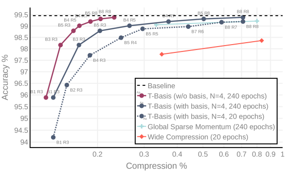
Figure 3: Top1 Accuracy vs. Model Compression Ratio for LeNet5 on MNIST classification. Each data point is annotated with basis size and rank. Our method outperforms in-place Tensor Ring weights allocation scheme and Global Sparse Momentum under extended training protocol. Legend: Wide Compression (TR) (Wang et al., 2018), Global Sparse Momentum SGD (Ding et al., 2019)

5.1 A Note on the Training Time

Training protocols of reference CNNs are designed with respect to convergence rates of the uncompressed models (He et al., 2016; Simonyan & Zisserman, 2015). Many works (Chen et al., 2018b) bootstrap existing feature extractors pre-trained on ImageNet (Krizhevsky et al., 2012), which helps them to reduce training time (He et al., 2019).

In most neural network compression formulations, customized architectures cannot be easily initialized with pre-trained weights. Hence longer training time is required for compressed models to bridge the gap with reference models. The increases in training time seen in the prior art can be as high as 12$\times$ (Ding et al., 2019); others report results of training until convergence (Eban et al., 2020).

Following this practice, we report the performance of a few experiments under the extended training protocol and conclude that longer training time helps our models in the absence of a better than random initialization.

5.2 Small Networks: LeNet5 on MNIST

We follow the training protocol explained in (Wang et al., 2018): 20 epochs, batch size 128, network architecture with two convolutional layers with 20 and 50 output channels respectively, and two linear layers with 320 and 10 output channels, a total of 429K in uncompressed parameters. Fig. 3 demonstrates performance of the specified LeNet5 architecture (LeCun et al., 1998) and T-Basis parameterization with various basis sizes and ranks. When training for 240 epochs, significant performance improvements are observed, and the model becomes competitive with (Ding et al., 2019), using the same extended training protocol.

Ablation Study: Pseudo-random T-Basis

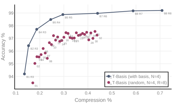
Figure 4: Comparison of learned and pseudo-random T-Basis approaches on MNIST digits classification with LeNet5. The performance of the learned basis cannot be reached by the pRNG basis, even with a large basis size (shown in datapoints annotations).

A natural question arises whether T-Basis basis needs to be a part of the learned parameters – perhaps we could initialize it with a pseudo-random numbers generator (pRNG) with a fixed seed (the fourth integer value describing all elements of such T-Basis other than B, R, and N) and only learn $\bm{\alpha}$ and $\bm{\rho}$ parameters? Fig. 4 attempts to answer this question. In short, pRNG T-Basis approach is further away from the optimality frontier than its learned counterpart.

5.3 Medium Networks: ResNets on CIFAR Datasets

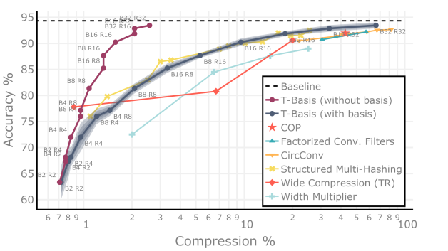
Figure 5: Top1 Accuracy vs. Model Compression Ratio for ResNet-32 on CIFAR-10 image classification. Shaded areas correspond to confidence intervals for one, two, and three standard deviations, computed over 10 runs. Our method outperforms in-place Tensor Ring weights allocation scheme (Wang et al., 2018), and is on par or better than other state-of-the-art methods. Legend: COP (Wang et al., 2019), Factorized Conv. Filters (Li et al., 2019a), CircConv (Liao & Yuan, 2019), Structured Multi-Hashing (Eban et al., 2020), Wide Compression (TR) (Wang et al., 2018), Width Multiplier (Eban et al., 2020).

CIFAR-10 (Krizhevsky & Hinton, 2009) and ResNet-32 (He et al., 2016) are arguably the most common combination seen in network compression works. This dataset consists of 60K RGB images of size 32x32, split into 50K train and 10K test splits. ResNet32 consists of a total of 0.46M parameters. Similarly to the prior art, we train our experiments until convergence (for 1000 epochs) with batch size 128, initial learning rate 0.1, and 50%-75% step LR schedule with gamma 0.1. The results are shown in Fig. 5 for the standard compression ratio evaluation protocol, and in Fig. 6 for the protocol which accounts for incompressible buffers. As in the previous case, our method outperforms in-place Tensor Ring weights allocation scheme (Wang et al., 2018) and is on par or better than other state-of-the-art methods. It is worth noting that the line “T-Basis w/o basis” contains vertical segments, corresponding to pairs of points with $(B,R)=(X,Y)$ and $(B,R)=(Y,X)$, with larger rank consistently giving a better score.

Ablation Study: Rank Adapters

Experimenting with different activation functions applied to the rank adapters values revealed that $\mathrm{exp}$ function yields the best results. No rank adaptation incurred $\sim$1% drop of performance in experiments with ResNet-32 on CIFAR-10.

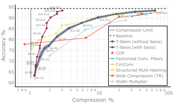
Figure 6: Top1 Accuracy vs. Model Compression Ratio for ResNet-32 on CIFAR-10 image classification. In this plot, T-Basis compression ratio is computed for compressible and incompressible parameters, and incompressible buffers, such as batchnorm statistics. Compression Limit denotes the ratio of incompressible and original network sizes. Wide Compression (TR) reports one point with smaller ratio than the limit, and Structured Multihashing reports one experiment right on the limit, suggesting that at least both of these methods report conventional compression ratios as explained in Sec. 5. The rest of the legend is the same as in Fig. 5.

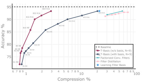
Figure 7: Top1 Accuracy vs. Model Compression Ratio for ResNet-56 on CIFAR-10 classification. Legend: Factorized Conv. Filters (Li et al., 2019a), Filter Distillation (Cuadros et al., 2020), Learning Filter Basis (Li et al., 2019b).

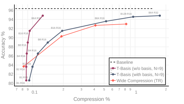
Figure 8: Top1 Accuracy vs. Model Compression Ratio for WRN-28-10 on CIFAR-10 classification. Legend: Wide Compression (TR) (Wang et al., 2018).

Table 1: Comparison of T-Basis with Tensor Ring Nets (Wang et al., 2018) compressing (w/ Basis) WRN-28-10 on CIFAR-100.

Method	Top1 Acc.	Compress. %
T-Basis ($B32$ $R8$)	$57.64$	$\mathbf{0.149}$
T-Basis ($B32$ $R8$ w/o B.)	$57.64$	$\mathbf{0.098}$
TR	$56.1$	$0.239$
Baseline	$78.3$	$100$

ResNet-56

ResNet56 consists of a total of 0.85M uncompressed parameters. In order to compare with the results of (Li et al., 2019b), who also capitalize on the basis representation, we comply with their training protocol and train for 300 epochs. Results are presented in Fig. 7. It can be seen that T-Basis is on par with “Learning Filter Basis”, and outperforms other state-of-the-art by a significant margin.

WideResNet-28-10

WRN-28-10 is an enhanced ResNet architecture (Zagoruyko & Komodakis, 2016); it contains 36.5M uncompressed parameters, which is considered a heavy-duty network. We compare with (Wang et al., 2018) in Table 1 and Fig. 8 in the extreme compression regime.

5.4 Large Networks: DeepLabV3+ on Pascal VOC

DeepLabV3+ (Chen et al., 2018b) is a standard network for semantic segmentation. We choose ResNet-34 backbone as a compromise between the model capacity and performance. Pascal VOC (Everingham et al., 2010) and SBD (Hariharan et al., 2011) datasets are often used together as a benchmark for semantic segmentation task. They are composed of 10582 photos in the training and 1449 photos in the validation splits and their dense semantic annotations with 21 classes. We train for 360K steps, original polynomial LR, batch size 16, crops 384$\times$384, without preloading ImageNet weights to make comparison with the baseline fair.

Table 2: mIoU vs. Model Compression Ratio (w/ Basis) for DeepLabV3+ on VOC+SBD semantic segmentation. Confidence interval: $mean\raisebox{0.86108pt}{$\scriptstyle\pm$}std$ over 3 runs.

Method	mIoU	Compress. %
T-Basis ($B128$ $R16$)	$58.18\raisebox{0.86108pt}{$\scriptstyle\pm$}0.69$	$1.450$
T-Basis ($B128$ $R32$)	$63.07\raisebox{0.86108pt}{$\scriptstyle\pm$}0.08$	$4.777$
Baseline	$64.08\raisebox{0.86108pt}{$\scriptstyle\pm$}0.59$	$100.0$

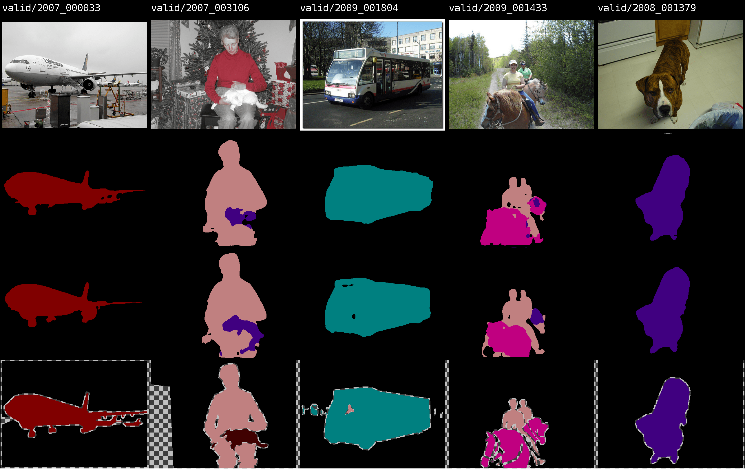
Figure 9: Semantic Segmentation predictions for a few images from Pascal VOC dataset validation split, made by a DeepLabV3+ model with ResNet-34 backbone, and 21$\times$ reduction in the number of parameters. Top to bottom: Input image, prediction by the compressed model, prediction by baseline, ground truth.

Our best results (see Table 2) for semantic segmentation are 1% away from the baseline with $<$5% of weights. A few visualizations from the validation split can be found in Fig. 9. We conclude that transitioning from toy datasets and models to large ones requires ranks $\geq 32$ in order to maintain performance close to the baseline.

6 Conclusion

We introduced a novel concept for compressing neural networks through a compact representation termed T-Basis. Motivated by the uniform weights sharing criterion and the low-rank Tensor Ring decomposition, our parameterization allows for efficient representation of Neural Networks weights through a shared basis and a few layer-specific coefficients. We demonstrate that our method can be used on top of the existing neural network architectures, such as ResNets, and introduces just two global hyperparameters – basis size and rank. Finally, T-Basis parameterization supports a broad range of compression ratios and provides a new degree of freedom to transfer the basis to other networks and tasks. We further study low-rank weight matrix parameterizations in the context of neural network training stability in our follow-up work (Obukhov et al., 2021).

References

- Alvarez & Salzmann (2016) Alvarez, J. M. and Salzmann, M. Learning the number of neurons in deep networks. In Advances in Neural Information Processing Systems, pp. 2270–2278, 2016.
- Ba & Caruana (2014) Ba, J. and Caruana, R. Do deep nets really need to be deep? In Advances in neural information processing systems, pp. 2654–2662, 2014.
- Chen et al. (2018a) Chen, L.-C., Zhu, Y., Papandreou, G., Schroff, F., and Adam, H. Encoder-decoder with atrous separable convolution for semantic image segmentation. In Proceedings of the European conference on computer vision (ECCV), pp. 801–818, 2018a.
- Chen et al. (2018b) Chen, L.-C., Zhu, Y., Papandreou, G., Schroff, F., and Adam, H. Encoder-decoder with atrous separable convolution for semantic image segmentation. In Proceedings of the European conference on computer vision (ECCV), pp. 801–818, 2018b.
- Chen et al. (2015) Chen, W., Wilson, J., Tyree, S., Weinberger, K., and Chen, Y. Compressing neural networks with the hashing trick. In International conference on machine learning, pp. 2285–2294, 2015.
- Courbariaux et al. (2015) Courbariaux, M., Bengio, Y., and David, J.-P. Binaryconnect: Training deep neural networks with binary weights during propagations. In Advances in neural information processing systems, pp. 3123–3131, 2015.
- Courbariaux et al. (2016) Courbariaux, M., Hubara, I., Soudry, D., El-Yaniv, R., and Bengio, Y. Binarized neural networks: Training deep neural networks with weights and activations constrained to+ 1 or-1. arXiv preprint arXiv:1602.02830, 2016.
- Cuadros et al. (2020) Cuadros, X. S., Zappella, L., and Apostoloff, N. Filter distillation for network compression. In The IEEE Winter Conference on Applications of Computer Vision (WACV), March 2020.
- Denil et al. (2013) Denil, M., Shakibi, B., Dinh, L., Ranzato, M., and De Freitas, N. Predicting parameters in deep learning. In Advances in neural information processing systems, pp. 2148–2156, 2013.
- Denton et al. (2014) Denton, E. L., Zaremba, W., Bruna, J., LeCun, Y., and Fergus, R. Exploiting linear structure within convolutional networks for efficient evaluation. In Advances in neural information processing systems, pp. 1269–1277, 2014.
- Devlin et al. (2019) Devlin, J., Chang, M.-W., Lee, K., and Toutanova, K. BERT: Pre-training of deep bidirectional transformers for language understanding. In Proceedings of the 2019 Conference of the North American Chapter of the Association for Computational Linguistics: Human Language Technologies, Volume 1 (Long and Short Papers), pp. 4171–4186, Minneapolis, Minnesota, June 2019. Association for Computational Linguistics. doi: 10.18653/v1/N19-1423.
- Ding et al. (2019) Ding, X., Zhou, X., Guo, Y., Han, J., Liu, J., et al. Global sparse momentum sgd for pruning very deep neural networks. In Advances in Neural Information Processing Systems, pp. 6379–6391, 2019.
- Eban et al. (2020) Eban, E., Movshovitz-Attias, Y., Wu, H., Sandler, M., Poon, A., Idelbayev, Y., and Carreira-Perpinan, M. A. Structured multi-hashing for model compression. In IEEE/CVF Conference on Computer Vision and Pattern Recognition (CVPR), June 2020.
- Espig et al. (2011) Espig, M., Hackbusch, W., Handschuh, S., and Schneider, R. Optimization problems in contracted tensor networks. Comput. Visual. Sci., 14(6):271–285, 2011. doi: 10.1007/s00791-012-0183-y.
- Everingham et al. (2010) Everingham, M., Van Gool, L., Williams, C. K. I., Winn, J., and Zisserman, A. The pascal visual object classes (voc) challenge. International Journal of Computer Vision, 88(2):303–338, June 2010.
- Faraone et al. (2018) Faraone, J., Fraser, N., Blott, M., and Leong, P. H. Syq: Learning symmetric quantization for efficient deep neural networks. In Proceedings of the IEEE Conference on Computer Vision and Pattern Recognition, pp. 4300–4309, 2018.
- Frankle & Carbin (2019) Frankle, J. and Carbin, M. The lottery ticket hypothesis: Finding sparse, trainable neural networks. In ICLR. OpenReview.net, 2019.
- Garipov et al. (2016) Garipov, T., Podoprikhin, D., Novikov, A., and Vetrov, D. Ultimate tensorization: compressing convolutional and fc layers alike. arXiv preprint arXiv:1611.03214, 2016.
- Gordon et al. (2018) Gordon, A., Eban, E., Nachum, O., Chen, B., Wu, H., Yang, T.-J., and Choi, E. Morphnet: Fast & simple resource-constrained structure learning of deep networks. In Proceedings of the IEEE Conference on Computer Vision and Pattern Recognition, pp. 1586–1595, 2018.
- Grasedyck et al. (2013) Grasedyck, L., Kressner, D., and Tobler, C. A literature survey of low-rank tensor approximation techniques. GAMM-Mitt., 36(1):53–78, 2013. doi: 10.1002/gamm.201310004.
- Graves et al. (2013) Graves, A., Mohamed, A.-r., and Hinton, G. Speech recognition with deep recurrent neural networks. In 2013 IEEE international conference on acoustics, speech and signal processing, pp. 6645–6649. IEEE, 2013.
- Han et al. (2015) Han, S., Pool, J., Tran, J., and Dally, W. Learning both weights and connections for efficient neural network. In Advances in Neural Information Processing Systems, pp. 1135–1143, 2015.
- Han et al. (2016) Han, S., Mao, H., and Dally, W. J. Deep compression: Compressing deep neural networks with pruning, trained quantization and huffman coding. In International Conference on Learning Representations, 2016.
- Hariharan et al. (2011) Hariharan, B., Arbelaez, P., Bourdev, L., Maji, S., and Malik, J. Semantic contours from inverse detectors. In International Conference on Computer Vision (ICCV), 2011.
- He et al. (2015) He, K., Zhang, X., Ren, S., and Sun, J. Delving deep into rectifiers: Surpassing human-level performance on imagenet classification. In 2015 IEEE International Conference on Computer Vision, ICCV 2015, Santiago, Chile, December 7-13, 2015, pp. 1026–1034. IEEE Computer Society, 2015. doi: 10.1109/ICCV.2015.123.
- He et al. (2016) He, K., Zhang, X., Ren, S., and Sun, J. Deep residual learning for image recognition. In Proceedings of the IEEE conference on computer vision and pattern recognition, pp. 770–778, 2016.
- He et al. (2017a) He, K., Gkioxari, G., Dollár, P., and Girshick, R. Mask r-cnn. In Proceedings of the IEEE international conference on computer vision, pp. 2961–2969, 2017a.
- He et al. (2019) He, K., Girshick, R., and Dollar, P. Rethinking imagenet pre-training. In The IEEE International Conference on Computer Vision (ICCV), October 2019.
- He et al. (2017b) He, Y., Zhang, X., and Sun, J. Channel pruning for accelerating very deep neural networks. In Proceedings of the IEEE International Conference on Computer Vision, pp. 1389–1397, 2017b.
- Hitchcock (1927) Hitchcock, F. L. The expression of a tensor or a polyadic as a sum of products. J. Math. Phys, 6(1):164–189, 1927.
- Jacob et al. (2018) Jacob, B., Kligys, S., Chen, B., Zhu, M., Tang, M., Howard, A., Adam, H., and Kalenichenko, D. Quantization and training of neural networks for efficient integer-arithmetic-only inference. In Proceedings of the IEEE Conference on Computer Vision and Pattern Recognition, pp. 2704–2713, 2018.
- Jaderberg et al. (2014) Jaderberg, M., Vedaldi, A., and Zisserman, A. Speeding up convolutional neural networks with low rank expansions. In Proceedings of the British Machine Vision Conference. BMVA Press, 2014.
- Kamnitsas et al. (2017) Kamnitsas, K., Ledig, C., Newcombe, V. F., Simpson, J. P., Kane, A. D., Menon, D. K., Rueckert, D., and Glocker, B. Efficient multi-scale 3d cnn with fully connected crf for accurate brain lesion segmentation. Medical image analysis, 36:61–78, 2017.
- Khoromskij (2011) Khoromskij, B. N. –Quantics approximation of – tensors in high-dimensional numerical modeling. Constr. Approx., 34(2):257–280, 2011. doi: 10.1007/s00365-011-9131-1.
- Kim et al. (2016) Kim, Y., Park, E., Yoo, S., Choi, T., Yang, L., and Shin, D. Compression of deep convolutional neural networks for fast and low power mobile applications. In Bengio, Y. and LeCun, Y. (eds.), 4th International Conference on Learning Representations, ICLR 2016, San Juan, Puerto Rico, May 2-4, 2016, Conference Track Proceedings, 2016.
- Kingma & Ba (2015) Kingma, D. P. and Ba, J. Adam: A method for stochastic optimization. In Bengio, Y. and LeCun, Y. (eds.), 3rd International Conference on Learning Representations, ICLR 2015, San Diego, CA, USA, May 7-9, 2015, Conference Track Proceedings, 2015.
- Kolda & Bader (2009) Kolda, T. G. and Bader, B. W. Tensor decompositions and applications. SIAM Rev., 51(3):455–500, 2009. doi: 10.1137/07070111X.
- Krizhevsky & Hinton (2009) Krizhevsky, A. and Hinton, G. Learning multiple layers of features from tiny images. Master’s thesis, Department of Computer Science, University of Toronto, 2009.
- Krizhevsky et al. (2012) Krizhevsky, A., Sutskever, I., and Hinton, G. E. Imagenet classification with deep convolutional neural networks. In Advances in neural information processing systems, pp. 1097–1105, 2012.
- Lebedev et al. (2015) Lebedev, V., Ganin, Y., Rakhuba, M., Oseledets, I. V., and Lempitsky, V. S. Speeding-up convolutional neural networks using fine-tuned cp-decomposition. In ICLR (Poster), 2015.
- LeCun et al. (1998) LeCun, Y., Bottou, L., Bengio, Y., and Haffner, P. Gradient-based learning applied to document recognition. Proceedings of the IEEE, 86(11):2278–2324, 1998.
- Li et al. (2017) Li, H., Kadav, A., Durdanovic, I., Samet, H., and Graf, H. P. Pruning filters for efficient convnets. In International Conference on Learning Representations, 2017.
- Li et al. (2019a) Li, T., Wu, B., Yang, Y., Fan, Y., Zhang, Y., and Liu, W. Compressing convolutional neural networks via factorized convolutional filters. In Proceedings of the IEEE Conference on Computer Vision and Pattern Recognition, pp. 3977–3986, 2019a.
- Li et al. (2019b) Li, Y., Gu, S., Gool, L. V., and Timofte, R. Learning filter basis for convolutional neural network compression. In Proceedings of the IEEE International Conference on Computer Vision, pp. 5623–5632, 2019b.
- Liao & Yuan (2019) Liao, S. and Yuan, B. Circconv: A structured convolution with low complexity. In Proceedings of the AAAI Conference on Artificial Intelligence, volume 33, pp. 4287–4294, 2019.
- Liu et al. (2017) Liu, Z., Li, J., Shen, Z., Huang, G., Yan, S., and Zhang, C. Learning efficient convolutional networks through network slimming. In Proceedings of the IEEE International Conference on Computer Vision, pp. 2736–2744, 2017.
- Liu et al. (2019) Liu, Z., Sun, M., Zhou, T., Huang, G., and Darrell, T. Rethinking the value of network pruning. In International Conference on Learning Representations, 2019.
- Nagel et al. (2019) Nagel, M., Baalen, M. v., Blankevoort, T., and Welling, M. Data-free quantization through weight equalization and bias correction. In Proceedings of the IEEE International Conference on Computer Vision, pp. 1325–1334, 2019.
- Novikov et al. (2015) Novikov, A., Podoprikhin, D., Osokin, A., and Vetrov, D. P. Tensorizing neural networks. In Advances in neural information processing systems, pp. 442–450, 2015.
- Obukhov et al. (2021) Obukhov, A., Rakhuba, M., Liniger, A., Huang, Z., Georgoulis, S., Dai, D., and Van Gool, L. Spectral tensor train parameterization of deep learning layers. In Banerjee, A. and Fukumizu, K. (eds.), Proceedings of The 24th International Conference on Artificial Intelligence and Statistics, volume 130 of Proceedings of Machine Learning Research, pp. 3547–3555. PMLR, 13–15 Apr 2021.
- Orús (2019) Orús, R. Tensor networks for complex quantum systems. Nature Reviews Physics, 1(9):538–550, 2019.
- Oseledets (2011) Oseledets, I. V. Tensor-train decomposition. SIAM Journal on Scientific Computing, 33(5):2295–2317, 2011.
- Paszke et al. (2019) Paszke, A., Gross, S., Massa, F., Lerer, A., Bradbury, J., Chanan, G., Killeen, T., Lin, Z., Gimelshein, N., Antiga, L., Desmaison, A., Kopf, A., Yang, E., DeVito, Z., Raison, M., Tejani, A., Chilamkurthy, S., Steiner, B., Fang, L., Bai, J., and Chintala, S. Pytorch: An imperative style, high-performance deep learning library. In Advances in Neural Information Processing Systems 32, pp. 8024–8035. Curran Associates, Inc., 2019.
- Peng et al. (2018) Peng, B., Tan, W., Li, Z., Zhang, S., Xie, D., and Pu, S. Extreme network compression via filter group approximation. In Proceedings of the European Conference on Computer Vision (ECCV), pp. 300–316, 2018.
- Perez-Garcia et al. (2007) Perez-Garcia, D., Verstraete, F., Wolf, M. M., and Cirac, J. I. Matrix product state representations. Quantum Info. Comput., 7(5):401–430, July 2007. ISSN 1533-7146.
- Rastegari et al. (2016) Rastegari, M., Ordonez, V., Redmon, J., and Farhadi, A. Xnor-net: Imagenet classification using binary convolutional neural networks. In European conference on computer vision, pp. 525–542. Springer, 2016.
- Reagan et al. (2018) Reagan, B., Gupta, U., Adolf, B., Mitzenmacher, M., Rush, A., Wei, G.-Y., and Brooks, D. Weightless: Lossy weight encoding for deep neural network compression. In Dy, J. and Krause, A. (eds.), Proceedings of the 35th International Conference on Machine Learning, volume 80 of Proceedings of Machine Learning Research, pp. 4324–4333, Stockholmsmässan, Stockholm Sweden, 10–15 Jul 2018. PMLR.
- Redmon et al. (2016) Redmon, J., Divvala, S., Girshick, R., and Farhadi, A. You only look once: Unified, real-time object detection. In Proceedings of the IEEE conference on computer vision and pattern recognition, pp. 779–788, 2016.
- Ronneberger et al. (2015) Ronneberger, O., Fischer, P., and Brox, T. U-net: Convolutional networks for biomedical image segmentation. In International Conference on Medical image computing and computer-assisted intervention, pp. 234–241. Springer, 2015.
- Simonyan & Zisserman (2015) Simonyan, K. and Zisserman, A. Very deep convolutional networks for large-scale image recognition. In Bengio, Y. and LeCun, Y. (eds.), 3rd International Conference on Learning Representations, ICLR 2015, San Diego, CA, USA, May 7-9, 2015, Conference Track Proceedings, 2015.
- Spring & Shrivastava (2017) Spring, R. and Shrivastava, A. Scalable and sustainable deep learning via randomized hashing. In Proceedings of the 23rd ACM SIGKDD International Conference on Knowledge Discovery and Data Mining, pp. 445–454, 2017.
- Su et al. (2018) Su, J., Li, J., Bhattacharjee, B., and Huang, F. Tensorial neural networks: Generalization of neural networks and application to model compression. arXiv preprint arXiv:1805.10352, 2018.
- Tucker (1963) Tucker, L. Implications of factor analysis of three-way matrices for measurement of change. Problems in measuring change, pp. 122–137, 1963.
- Wang et al. (2017) Wang, W., Aggarwal, V., and Aeron, S. Efficient low rank tensor ring completion. In Proceedings of the IEEE International Conference on Computer Vision, pp. 5697–5705, 2017.
- Wang et al. (2018) Wang, W., Sun, Y., Eriksson, B., Wang, W., and Aggarwal, V. Wide compression: Tensor ring nets. In Proceedings of the IEEE Conference on Computer Vision and Pattern Recognition, pp. 9329–9338, 2018.
- Wang et al. (2019) Wang, W., Fu, C., Guo, J., Cai, D., and He, X. Cop: Customized deep model compression via regularized correlation-based filter-level pruning. In Proceedings of the Twenty-Eighth International Joint Conference on Artificial Intelligence, IJCAI-19, pp. 3785–3791. International Joint Conferences on Artificial Intelligence Organization, 7 2019. doi: 10.24963/ijcai.2019/525.
- Wen et al. (2016) Wen, W., Wu, C., Wang, Y., Chen, Y., and Li, H. Learning structured sparsity in deep neural networks. In Advances in neural information processing systems, pp. 2074–2082, 2016.
- Wu et al. (2016) Wu, J., Leng, C., Wang, Y., Hu, Q., and Cheng, J. Quantized convolutional neural networks for mobile devices. In Proceedings of the IEEE Conference on Computer Vision and Pattern Recognition, pp. 4820–4828, 2016.
- Yang et al. (2018) Yang, T.-J., Howard, A., Chen, B., Zhang, X., Go, A., Sandler, M., Sze, V., and Adam, H. Netadapt: Platform-aware neural network adaptation for mobile applications. In Proceedings of the European Conference on Computer Vision (ECCV), pp. 285–300, 2018.
- Yu et al. (2018) Yu, R., Li, A., Chen, C.-F., Lai, J.-H., Morariu, V. I., Han, X., Gao, M., Lin, C.-Y., and Davis, L. S. Nisp: Pruning networks using neuron importance score propagation. In Proceedings of the IEEE Conference on Computer Vision and Pattern Recognition, pp. 9194–9203, 2018.
- Zagoruyko & Komodakis (2016) Zagoruyko, S. and Komodakis, N. Wide residual networks. In Proceedings of the British Machine Vision Conference (BMVC), pp. 87.1–87.12. BMVA Press, September 2016. doi: 10.5244/C.30.87.
- Zhang et al. (2015) Zhang, X., Zou, J., He, K., and Sun, J. Accelerating very deep convolutional networks for classification and detection. IEEE transactions on pattern analysis and machine intelligence, 38(10):1943–1955, 2015.
- Zhao et al. (2016) Zhao, Q., Zhou, G., Xie, S., Zhang, L., and Cichocki, A. Tensor ring decomposition. arXiv preprint arXiv:1606.05535, 2016.
- Zhou et al. (2016a) Zhou, H., Alvarez, J. M., and Porikli, F. Less is more: Towards compact cnns. In European Conference on Computer Vision, pp. 662–677. Springer, 2016a.
- Zhou et al. (2016b) Zhou, S., Wu, Y., Ni, Z., Zhou, X., Wen, H., and Zou, Y. Dorefa-net: Training low bitwidth convolutional neural networks with low bitwidth gradients. arXiv preprint arXiv:1606.06160, 2016b.
- Zhu et al. (2017) Zhu, C., Han, S., Mao, H., and Dally, W. J. Trained ternary quantization. In 5th International Conference on Learning Representations, ICLR 2017, Toulon, France, April 24-26, 2017, Conference Track Proceedings. OpenReview.net, 2017.