Analysis of Red-Supergiants in VdBH 222

Abstract

Recent surveys uncovered new Young Massive Clusters (YMCs) that host dozens of Red Supergiants (RSGs) in the inner Milky Way. These clusters are ideal for studying the most recent and violent star formation events in the inner Galaxy. However, due to the high extinction that affects the Galactic plane, they need to be studied through infrared (IR) spectroscopy. IR spectra of RSGs have proven to be powerful tools for obtaining chemical abundances.
We present the first [Fe$/$H] measurement ($-$0.07$\pm$0.02) for the YMC VdBH 222 through analysis of its RSGs using VLT/X-shooter spectra. We find no evidence for Multiple Stellar Populations (MSPs) in this YMC, contrary to what is routinely observed in older massive clusters.

1 Introduction and Motivation

Accurate information about the abundances of different elements reveal information about the star formation and chemical enrichment history of the host galaxy (i.e. Matteucci, 2012, and references therein). Additionally, determining the abundances of elements resulting from different nucleosynthesis processes such as Type I supernovae (producing Fe-peak elements: Sc, V, Cr, Mn, Fe, Co and Ni), core collapse supernovae (producing $\alpha$-elements: O, Ne, Mg, Si S, Ar, Ca and Ti) and winds from evolved stars can provide us with information about these complex mechanisms.
The chemical enrichment history of the Galactic center is a crucial matter to unveil the Galaxy’s evolution.

The Galactic center has experienced a recent rich star-forming activity which formed numerous young star clusters dominated by red supergiants and large number of massive stars observed there. The origin of this activity can be traced by the metallicity and chemical abundances of these young objects (Figer et al., 1999, 2002; Stolte et al., 2014).
Star clusters lie at the heart of modern astrophysics because they can provide information both about the chemical evolution of their host galaxy as well as the stellar evolution of their constituent stars (Bertelli et al., 2003; Brodie & Strader, 2006; Gratton et al., 2019). Studies of massive star clusters of different ages has received further boost after the discovery of ubiquitous presence of Multiple Stellar Populations (MSP) phenomenon, defined as star-to-star variation of light element (He, C, N, O, Na, Al) abundances, in old Milky Way clusters (e.g. Carretta et al., 2009), which has changed our view of star clusters as simple stellar populations. The origin of the MSP phenomenon is still poorly understood. For the recent review see Bastian & Lardo (2018).
Larsen et al. (2006) analyzed the chemical abundances and abundance patterns with near-infrared spectroscopy in a young cluster. Several studies (Davies et al., 2010, 2015; Patrick et al., 2016) demonstrated that the IR spectra of red supergiants (RSGs) can be used to measure abundances. Gazak et al. (2014) showed that the technique works down to resolving powers of R = 3000. RSGs are cool ($\sim$ 4000 K), highly luminous ($\sim$ $10^{5}$ L_⊙) stars of spectral class K and M with masses between 10 to 30 M_⊙. They are evolved stars that left the main sequence but they are young ($<$20 Myr) and have short lifetimes (Levesque, 2010).
Cabrera-Ziri et al. (2016); Lardo et al. (2017) used the integrated spectra of Young Massive Clusters (YMC) in the J-band (1.1 to 1.4 $\mu$m) which is dominated by RSG to search for evidence for MSP in star of different masses (while previous studies mostly focused on low-mass stars). Studies covering a broader sample of clusters will help answering long standing questions like: are YMCs and Globular Clusters (GCs) objects of the same nature? Do both share the peculiar abundance patterns?
In this work we analyse the YMC VdBH 222 (SIMBAD identifier: Cl VDBH 222), located in the inner Milky Way, found by van den Bergh & Hagen (1975). This cluster is ideal for this type of study as it is one of the few stellar clusters with confirmed RSGs. Due to the high extinction that affects the Galactic plane, stars in VdBH 222 need to be studied through IR spectroscopy. Piatti & Clariá (2002) estimated an age of 60$\pm$30 Myr for it and concluded that it would be important to derive the cluster metallicity in order to improve our knowledge of the radial metal abundance gradient and the age-metallicity relation for the disk of our Galaxy.
Marco et al. (2014) characterised this cluster using a comprehensive set of multi-wavelength observations and determined a reddening E(B-V) of 2.45 $\pm$ 0.15 using non-standard extinction law with a value of R = 2.9 and an age range of 12$-$16 Myr at a distance of 7$-$10 kpc. They confirmed that this YMC has a likely mass of 2x10⁴M_⊙, and that it is an extremely compact cluster with very few members lying outside a radius of 1.5’ from the cluster’s center. They pointed that VdBH 222 is much closer to the Galactic centre (and so to the nominal tip of the bar) than other massive clusters reported in the area (Davies et al., 2012; Ramírez Alegría et al., 2014). Clark et al. (2015) inferred a distance of about 6kpc for VdBH 222 and an age of about 20 Myr.
Marco et al. (2014) identified nine RSG in this cluster and derived an average radial velocity v${}_{LSR}=-$99$\pm$4 km s^-1. In their analysis of open cluster kinematics with Gaia DR2, Soubiran et al. (2018) derived a radial velocity of $-$119.3$\pm$2.8 km s^-1 based on five stars.
Using X-shooter at the Very Large Telescope (VLT) IR data, we provide the first estimate of the properties and iron abundance of six RSG in this cluster. We also search for evidence of MSP through analysis of [Al/Fe].
The paper is organized as follows: in section 2 we describe our observations and the data reduction. In section 3 we discuss the models and the method used, in section 4 we provide details about the error analysis and in section 5 we present our results. In section 6 we shed light on the Multiple Stellar Populations phenomenon in this cluster. The conclusion is provided in section 7.

2 Observations and Data Reduction

We obtained the IR spectra of six RSGs in VdBH 222 using VLT/X-shooter (D’Odorico et al., 2006; Vernet et al., 2011) in service mode under ESO programme number 0103.D-0881(A) (PI R. Asad). These observations provide continuous spectral coverage from 0.3$-$2.4 $\mu$m. Integration times were chosen to achieve a signal-to-noise ratio (S/N) of at least 100 in the NIR. By examining the color-magnitude diagrams (CMDs) of the cluster we established that the RSGs are bright having K 6-8 mag. Hence with 2x30s integration in the NIR we were able to get S/N of a few hundreds. The sample of RSG stars for the cluster was assembled from Marco et al. (2014). We used the slits 1.0", 0.9", 0.9" for UVB, VIS and NIR channels, respectively. This gives a resolution higher that R$\sim$5600 in the NIR arm. The precise value of R for each RSGs is determined at the analysis stage. For this work we used the J-band spectra, that are dominated by atomic rather than molecular absorption, allowing accurate stellar abundances measurements (Davies et al., 2010, 2015). Details about the S$/$N of each cluster RSG target is given in Table 1. The average S$/$N of the clusters targets is 233.

We started with the advanced data products for our observed sample from the ESO archive. The spectra were processed by applying the standard spectroscopic data reduction steps as described in the associated data release description available on the ESO Phase 3 website.
We corrected the 1D extracted and flux-calibrated spectra for telluric absorption using molecfit (Smette et al., 2015; Kausch et al., 2015). We used the same approach as developed for the X-shooter Spectral Library (Gonneau et al., 2020). First we apply molecfit to the entire near-IR spectrum to derive the precipitable water vapour column (PWV). Then we divide the spectrum into smaller wavelength segments and apply molecfit locally using the PWV value determined before. The corrected wavelength segments are then merged together.

3 Models and Method

The kinematic parameters and chemical abundances were derived by comparing the observed spectra with synthetic spectra generated by the Payne spectral model (Ting et al., 2019), through a $\chi^{2}$ minimization in the wavelength range $11600-12200$ Å. As a training set for the Payne we adopted model atmospheres calculated with MARCS code (Gustafsson et al., 2008). The NLTE spectral grids were computed by Bergemann et al. (2015), using NLTE departures for Si, Ti and Fe lines from Bergemann et al. (2012b, a, 2013). This model is similar to the model used in Davies et al. (2015)
The parameter space includes stellar parameters (T_eff, log(g), microturbulence ($\xi$) and [Fe/H]) together with radial velocity, resolution and normalization coefficients for Chebyshev polynomials. The grid of models is computed for a range of T_eff between 3400 and 4400 K in steps of 100K, log(g) between $-$1.0 and $+$1.0 in steps of 0.25 (cgs units), $\xi$ from 1 to 5 km s^-1 and [Fe/H] between $-$ 1.0 and $+$1.0 dex is steps of 0.25 dex. The synthetic spectrum was shifted to radial velocity and degraded to the spectral resolution (using Gaussian filter) of observed stellar spectrum, which was normalized using linear combination of the first four Chebyshev polynomials (similar to Kovalev et al., 2019).

4 Error Analysis

In addition to the statistical errors associated with the fitting, we discuss the following errors: RMS from tests done on simulated mock stars and degeneracy errors. The total errors are taken to be the quadrature sum of the statistical errors from $\chi^{2}$ minimisation and the RMS from tests on simulated mock stars.

4.1 Tests on simulated mock stars

We use the Payne spectral model to create 100,000 mock stellar spectra (generated in random points within parameter’s space of original model grid) with Gaussian noise corresponding to $S/N=100$. All mock spectra were degraded to a resolution of $R=9700$ and shifted to random radial velocities from $-40$ to $40$ km s^-1. They were also multiplied by a polynomial function representing continuum placement uncertainty.
We then aimed to recover the original stellar parameters. The 4 panels of Figure 1 show the offset and scatter for each (output-input) versus (input) parameter. We use the bias (offset) from the expected value and RMS as the measure of the fitting performance. All parameters show negligible bias values. The RMS value is 19 K in $T_{eff}$, 0.1 dex in log(g), 0.04 dex in metallicity and 0.05 km s^-1 in $\xi$.

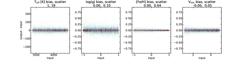
Figure 1: The distribution of the derived parameters for the set of mock stars. The black dots represent the sample of 100,000 mock stars, the red line is the central line. The bias and RMS are shown in panels’ titles.

4.2 Degeneracy

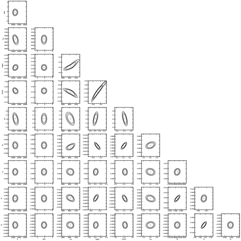
Figure 5: The contour plot showing degeneracies between parameters. They were obtained by changing two parameters at a time and keeping the rest fixed to the optimal values. Contour lines are shown for values corresponding to 1, 2, 3 $\sigma$ levels. Optimal parameters are shown with pluses.

To investigate the uncertainty caused by the degeneracies between estimated parameters, we calculate the $\chi^{2}$ values for $40000$ points around optimal solution, changing two parameters at time and keeping the other parameters fixed to the optimal values. The contour lines are shown in Figure 5 for values corresponding to 1, 2, 3 $\sigma$ levels. Optimal parameters are shown with pluses.
T0, T1 and T2 are the coefficients of Chebyshev polynomials used in normalisation. The figures are in agreement with the degeneracy analysis of Davies et al. (2015) who emphasized the degeneracy between [Fe/H] and log(g). Those uncertainties are already included in the statistical errors from $\chi^{2}$, because we fit for all parameters simultaneously. After each fit we obtain a covariance matrix from which we calculate the quadrature sum of diagonal elements as statistical errors.

5 Results

Figure 2 shows the best match between the observed RSGs and NLTE MARCS models when masking the regions of 1Å around points where the mean residuals are greater than 0.03. The numerical results are listed in Table 1. The ID of each star reflects the unique OB number given during the observing run.

Figure 2: The best match between the observed RSGs (black) and NLTE model (red) masking the regions of 1Å around points where the mean residuals are greater than 0.03 (grey shaded). Residuals are shown in green.

All RSGs have radial velocities within $\pm$3km s^-1 from each other which confirms that they are all members of the cluster. The average radial velocity for our sample is $-$116.5$\pm$3 km s^-1 which is consistent with the two values from other studies, $-$119.3$\pm$2.8 km s^-1 from Soubiran et al. (2018) based on their open cluster kinematics with Gaia DR2 and $-$99$\pm$4 km s^-1 obtained by Marco et al. (2014).

Star31 has the lowest temperature. Star61 has the highest temperature. The overall sequence in temperature values is consistent with the spectral classes identified for this sample by Marco et al. (2014).

In figure 3 we plot the Hertzsprung–Russell diagram (HRD) for this cluster using the temperatures we obtained for the RSGs in our sample. The NIR magnitudes are form the 2MASS catalogue. We use Padova (Bressan et al., 2012; Marigo et al., 2013; Pastorelli et al., 2019) 12Myr, 14Myr and 16 Myr isochrones with E(B$-$V) = 2.45 (values from Marco et al., 2014). The red, black and dark blue crosses correspond to distances of 7, 8 and 10 kpc respectively. The comparison of the new stellar parameters with the theoretical models favour older ages and shorted distances or $\sim$ 16Myr and D$\sim$8 kpc.

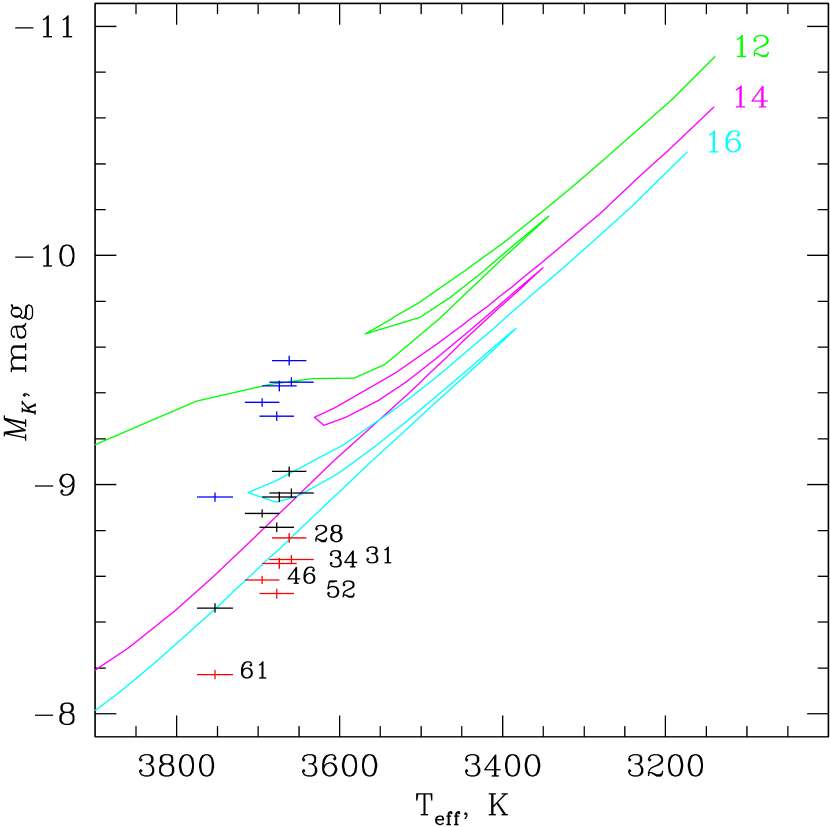
Figure 3: HRD for VdBH 222 using our RSG sample. The red, black and dark blue crosses correspond to distances of 7, 8 and 10 kpc, respectively. We use 12Myr, 14Myr and 16Myr isochrones with E(B$-$V)=2.45.

RSGs in our sample have temperatures in the 3650$-$3750 K range, surface gravity log(g) from $-$0.7 to $-$0.5 and microturbulence in the 2.6$-$2.8 km s^-1 range.

We find the average [Fe$/$H] to be $-$0.07$\pm$0.02. This is the first estimation of metallicity in this cluster. This value is in line with findings from other studies of RSGs in inner Milky Way (i.e. see discussions in Cunha et al., 2007; Ramírez et al., 2000; Carr et al., 2000; Davies et al., 2009b, a; Origlia et al., 2013, 2016, 2019).

6 Multiple Stellar Populations

It is well established now that globular clusters (GC) host multiple stellar populations (MSP; e.g., Milone et al., 2013, 2015, 2016, 2017, 2020; Bastian et al., 2015; Bastian & Lardo, 2018; Bastian et al., 2019, 2020, and references therein) inferred through star-to-star variations in the abundances of some light elements (e.g., He, C, N, O, Na, Al). Several scenarios have been proposed to explain this phenomenon, with most implying multiple epochs of star-formation within the cluster, however none have fully succeeded to reproduce the increasing number of observations obtained in the past decade. Hence, the origin of this phenomenon is still debated. Even more puzzling is the fact that no evidence of MSPs has been found so far in lower-mass ($<$ 10⁴ M${}_{\odot}\/$) open clusters nor in 1-2 Gyr massive ($>$ 10⁵ M${}_{\odot}\/$) clusters (Bastian & Lardo, 2018).
Marco et al. (2014) reports that VdBH 222 is almost certainly the most massive cluster observable in the U and B bands in the Milky Way. This makes it an ideal candidate to search for MSP, as several studies showed the there is a threshold of cluster mass for which MSPs can be observed (Carretta et al., 2010; Milone et al., 2017; Bastian et al., 2019).
In order to search for star-to-star light element abundance variations and quantitatively investigate the phenomenon of MSP in YMCs, we look for Al variations as Al lines in the wavelength range $13120-13155$ Å have been previously used in the literature to look for the presence of MSPs in the spectra of RSGs in young clusters (Cabrera-Ziri et al., 2016; Lardo et al., 2017).
Pancino et al. (2017) found that the extension of the Mg-Al anti-correlation (i.e. Al enhancement) depends on both metallicity and mass. Cabrera-Ziri et al. (2016) defined the [Al/Fe] spread as $\Delta$[Al$/$Fe]= mean([Al/Fe]) $-$ min([Al/Fe]) and divided the $\Delta$[Al$/$Fe] observed in GCs in three broad ranges: moderate, intermediate and extreme according to their $\Delta$[Al/Fe] values $\Delta$[Al/Fe]= 0.1, 0.3 and 0.7 dex, respectively.
We examine the Al variation in our cluster based on these ranges. The average best fitting values of [Al$/$Fe] for our RSG sample is 0.9 dex. In Figure 4 we show our observations overplotted with models of [Al/Fe] = 0.0, 0.5 and 1.0 respectively.
$\Delta$[Al/Fe] for our sample is 0.1 which is in the moderate range defined by Cabrera-Ziri et al. (2016). We infer that there is no evidence for MSP in this cluster, which is consistent with findings of other studies for clusters of this young age. As pointed by Cabrera-Ziri et al. (2016), this might be due to the fact that MPs only manifest themselves in low mass stars due to some evolutionary mechanism.

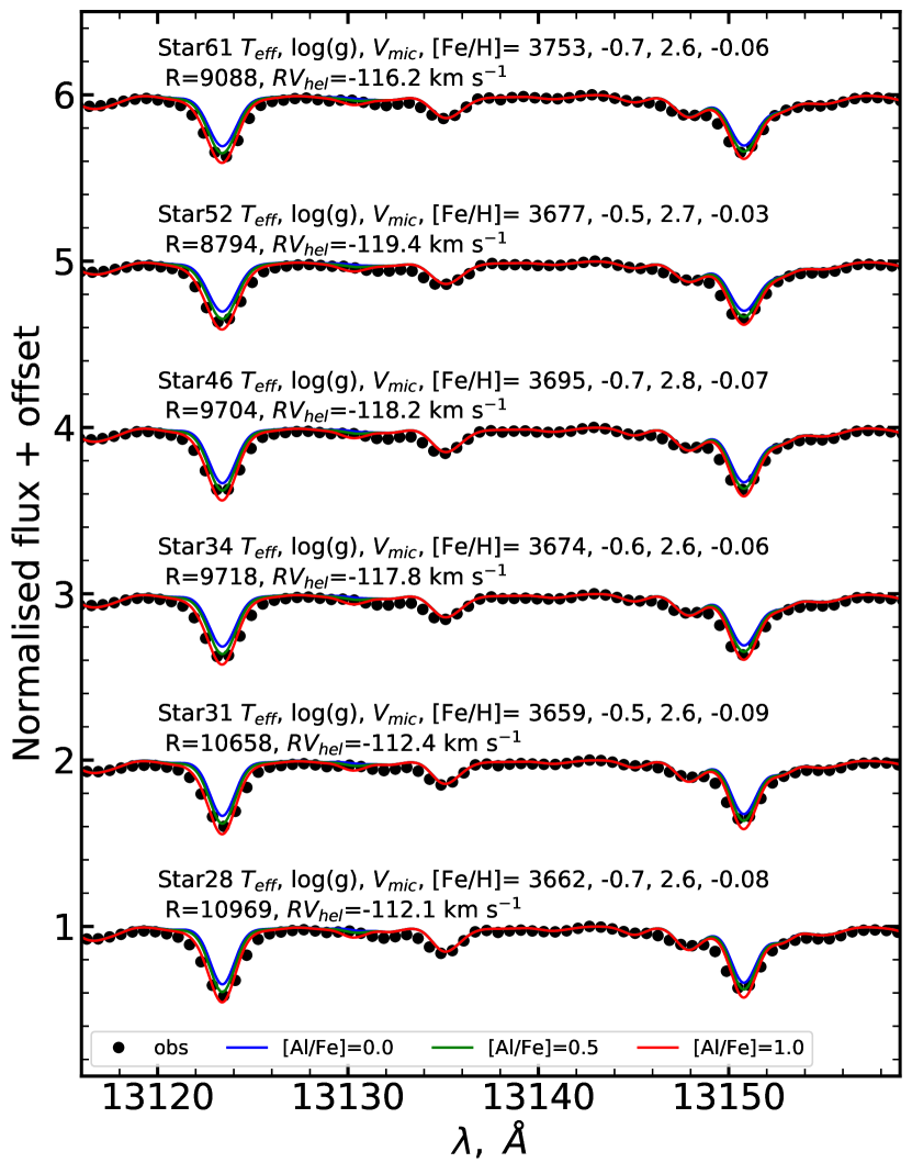
Figure 4: Comparing Al spectral line for each RSG in our sample with models of [Al/Fe] = 0.0, 0.5 and 1.0 respectively while keeping all other parameters derived in the previous section constant.

7 Conclusion

There are young massive clusters recently discovered in the central regions of the Milky Way that are still poorly characterised, requiring further study. One of them is our cluster VdBH 222.
Using (VLT)+X-shooter IR spectra ($11600-12200$ Å) of six RSGs in this clusters we apply the J-band full spectrum technique to derive the stellar parameters and abundances. Our results are summarized as follows:
1. The average radial velocity for our sample is $-$116.5$\pm$3 km s^-1 which is consistent with previous studies.
2. The RSGs of our sample have temperatures in the 3650$-$3750 K range. The order of the temperature values (hottest to coolest) are consistent with the spectral classes identified by Marco et al. (2014) for this sample.
3. Our sample has surface gravity log(g) in the $-$0.7 to $-$0.5 range and microturbulence in the 2.6 to 2.8 km s^-1 range.
4. We provide the first [Fe$/$H] estimate for this YMC. We find the average [Fe$/$H] to be $-$0.07$\pm$0.02 which is in line with findings from other studies for clusters in the central region of the MW.
5. In our search for Multiple Stellar Populations in this YMC, we exclude at high confidence extreme [Al/Fe] enhancements similar to those observed in GCs, hence we infer that this massive, extremely young, open cluster does not show MSPs. This is in line with other studies, as no evidence for MSPs has been yet observed in clusters younger than 2 Gyrs (Bastian & Lardo, 2018, and references therein). However, we need more observations in order to better understand if this is a property attributable to all young massive clusters or it is because MSPs only manifest themselves in low mass stars due to some evolutionary mechanism. The origin of MSPs is still unclear and further studies of young massive clusters may provide constraints for better understanding this phenomenon.
Our analysis of this cluster is based on the mass and age derived by Marco et al. (2014), where the cluster’s total mass was determined from its similitude with objects having comparable number of RSGs, not from star counts or other methods for membership determinations (like proper motions, parallaxes … etc). VdBH 222 was chosen for this study although it has not been previously studies comprehensively, because it is one of the few clusters with confirmed multiple RSGs. The uncertainty in the total cluster mass, age and distance should be noted. More accurate studies on this cluster are needed.

Table 1: Parameters and Abundances of the RSGs sample

ID	Res.	RV (km s-1)	RA	Dec	T${}_{eff}(K)$	log(g)	[Fe$/$H]	$\xi$	S$/$N
Star28	10969	-112.1	259.70310	-38.29149	3662$\pm$21	$-$0.7$\pm$0.1	$-$0.08$\pm$0.04	2.6$\pm$0.1	291
Star31	10658	-112.4	259.70198	-38.28356	3659$\pm$27	$-$0.5$\pm$0.1	$-$0.09$\pm$0.06	2.6$\pm$0.1	261
Star34	9718	-117.8	259.68680	-38.29786	3674$\pm$21	$-$0.6$\pm$0.1	$-$0.06$\pm$0.04	2.6$\pm$0.1	118
Star46	9704	-118.2	259.69237	-38.27003	3695$\pm$21	$-$0.7$\pm$0.1	$-$0.07$\pm$0.05	2.8$\pm$0.1	244
Star52	8794	-119.4	259.70270	-38.30095	3677$\pm$21	$-$0.5$\pm$0.1	$-$0.03$\pm$0.04	2.7$\pm$0.1	251
Star61	9088	-116.2	259.69552	-38.28856	3753$\pm$22	$-$0.7$\pm$0.1	$-$0.06$\pm$0.04	2.6$\pm$0.1	234
Mean Value	-	$-$116.5$\pm$3	-	-	3686$\pm$35	$-$0.6$\pm$0.1	$-$0.07$\pm$0.02	2.7$\pm$0.1	233

References

- Bastian et al. (2015) Bastian, N., Cabrera-Ziri, I., & Salaris, M. 2015, MNRAS, 449, 3333
- Bastian & Lardo (2018) Bastian, N., & Lardo, C. 2018, ARA&A, 56, 83
- Bastian et al. (2019) Bastian, N., Usher, C., Kamann, S., et al. 2019, MNRAS, 489, L80
- Bastian et al. (2020) Bastian, N., Lardo, C., Usher, C., et al. 2020, MNRAS, 494, 332
- Bergemann et al. (2015) Bergemann, M., Kudritzki, R.-P., Gazak, Z., Davies, B., & Plez, B. 2015, ApJ, 804, 113
- Bergemann et al. (2012a) Bergemann, M., Kudritzki, R.-P., Plez, B., et al. 2012a, ApJ, 751, 156
- Bergemann et al. (2013) Bergemann, M., Kudritzki, R.-P., Würl, M., et al. 2013, ApJ, 764, 115
- Bergemann et al. (2012b) Bergemann, M., Lind, K., Collet, R., Magic, Z., & Asplund, M. 2012b, MNRAS, 427, 27
- Bertelli et al. (2003) Bertelli, G., Nasi, E., Girardi, L., et al. 2003, AJ, 125, 770
- Bressan et al. (2012) Bressan, A., Marigo, P., Girardi, L., et al. 2012, MNRAS, 427, 127
- Brodie & Strader (2006) Brodie, J. P., & Strader, J. 2006, ARA&A, 44, 193
- Cabrera-Ziri et al. (2016) Cabrera-Ziri, I., Lardo, C., Davies, B., et al. 2016, MNRAS, 460, 1869
- Carr et al. (2000) Carr, J. S., Sellgren, K., & Balachandran, S. C. 2000, ApJ, 530, 307
- Carretta et al. (2010) Carretta, E., Bragaglia, A., Gratton, R. G., et al. 2010, A&A, 516, A55
- Carretta et al. (2009) —. 2009, A&A, 505, 117
- Clark et al. (2015) Clark, J. S., Negueruela, I., Lohr, M. E., et al. 2015, A&A, 584, L12
- Cunha et al. (2007) Cunha, K., Sellgren, K., Smith, V. V., et al. 2007, ApJ, 669, 1011
- Davies et al. (2012) Davies, B., de La Fuente, D., Najarro, F., et al. 2012, MNRAS, 419, 1860
- Davies et al. (2010) Davies, B., Kudritzki, R.-P., & Figer, D. F. 2010, MNRAS, 407, 1203
- Davies et al. (2015) Davies, B., Kudritzki, R.-P., Gazak, Z., et al. 2015, ApJ, 806, 21
- Davies et al. (2009a) Davies, B., Origlia, L., Kudritzki, R.-P., et al. 2009a, ApJ, 694, 46
- Davies et al. (2009b) —. 2009b, ApJ, 696, 2014
- D’Odorico et al. (2006) D’Odorico, S., Dekker, H., Mazzoleni, R., et al. 2006, Society of Photo-Optical Instrumentation Engineers (SPIE) Conference Series, Vol. 6269, X-shooter UV- to K-band intermediate-resolution high-efficiency spectrograph for the VLT: status report at the final design review, 626933
- Figer et al. (1999) Figer, D. F., McLean, I. S., & Morris, M. 1999, ApJ, 514, 202
- Figer et al. (2002) Figer, D. F., Najarro, F., Gilmore, D., et al. 2002, ApJ, 581, 258
- Gazak et al. (2014) Gazak, J. Z., Davies, B., Bastian, N., et al. 2014, ApJ, 787, 142
- Gonneau et al. (2020) Gonneau, A., Lyubenova, M., Lançon, A., et al. 2020, A&A, 634, A133
- Gratton et al. (2019) Gratton, R., Bragaglia, A., Carretta, E., et al. 2019, A&A Rev., 27, 8
- Gustafsson et al. (2008) Gustafsson, B., Edvardsson, B., Eriksson, K., et al. 2008, A&A, 486, 951
- Kausch et al. (2015) Kausch, W., Noll, S., Smette, A., et al. 2015, A&A, 576, A78
- Kovalev et al. (2019) Kovalev, M., Bergemann, M., Ting, Y.-S., & Rix, H.-W. 2019, A&A, 628, A54
- Lardo et al. (2017) Lardo, C., Cabrera-Ziri, I., Davies, B., & Bastian, N. 2017, MNRAS, 468, 2482
- Larsen et al. (2006) Larsen, S. S., Origlia, L., Brodie, J. P., & Gallagher, J. S. 2006, MNRAS, 368, L10
- Levesque (2010) Levesque, E. M. 2010, New A Rev., 54, 1
- Marco et al. (2014) Marco, A., Negueruela, I., González-Fernández, C., et al. 2014, A&A, 567, A73
- Marigo et al. (2013) Marigo, P., Bressan, A., Nanni, A., Girardi, L., & Pumo, M. L. 2013, MNRAS, 434, 488
- Matteucci (2012) Matteucci, F. 2012, Chemical Evolution of Galaxies, doi:10.1007/978-3-642-22491-1
- Milone et al. (2013) Milone, A. P., Bedin, L. R., Cassisi, S., et al. 2013, A&A, 555, A143
- Milone et al. (2016) Milone, A. P., Marino, A. F., D’Antona, F., et al. 2016, MNRAS, 458, 4368
- Milone et al. (2015) Milone, A. P., Bedin, L. R., Piotto, G., et al. 2015, MNRAS, 450, 3750
- Milone et al. (2017) Milone, A. P., Marino, A. F., D’Antona, F., et al. 2017, MNRAS, 465, 4363
- Milone et al. (2020) Milone, A. P., Marino, A. F., Da Costa, G. S., et al. 2020, MNRAS, 491, 515
- Origlia et al. (2013) Origlia, L., Oliva, E., Maiolino, R., et al. 2013, A&A, 560, A46
- Origlia et al. (2016) Origlia, L., Oliva, E., Sanna, N., et al. 2016, A&A, 585, A14
- Origlia et al. (2019) Origlia, L., Dalessandro, E., Sanna, N., et al. 2019, A&A, 629, A117
- Pancino et al. (2017) Pancino, E., Romano, D., Tang, B., et al. 2017, A&A, 601, A112
- Pastorelli et al. (2019) Pastorelli, G., Marigo, P., Girardi, L., et al. 2019, MNRAS, 485, 5666
- Patrick et al. (2016) Patrick, L. R., Evans, C. J., Davies, B., et al. 2016, MNRAS, 458, 3968
- Piatti & Clariá (2002) Piatti, A. E., & Clariá, J. J. 2002, A&A, 388, 179
- Ramírez et al. (2000) Ramírez, S. V., Sellgren, K., Carr, J. S., et al. 2000, ApJ, 537, 205
- Ramírez Alegría et al. (2014) Ramírez Alegría, S., Borissova, J., Chené, A. N., et al. 2014, A&A, 564, L9
- Smette et al. (2015) Smette, A., Sana, H., Noll, S., et al. 2015, A&A, 576, A77
- Soubiran et al. (2018) Soubiran, C., Cantat-Gaudin, T., Romero-Gómez, M., et al. 2018, A&A, 619, A155
- Stolte et al. (2014) Stolte, A., Hußmann, B., Morris, M. R., et al. 2014, ApJ, 789, 115
- Ting et al. (2019) Ting, Y.-S., Conroy, C., Rix, H.-W., & Cargile, P. 2019, ApJ, 879, 69
- van den Bergh & Hagen (1975) van den Bergh, S., & Hagen, G. L. 1975, AJ, 80, 11
- Vernet et al. (2011) Vernet, J., Dekker, H., D’Odorico, S., et al. 2011, A&A, 536, A105