Calculating the primary Lund Jet Plane density

Abstract

The Lund-jet plane has recently been proposed as a powerful jet substructure tool with a broad range of applications. In this paper, we provide an all-order single logarithmic calculation of the primary Lund-plane density in Quantum Chromodynamics, including contributions from the running of the coupling, collinear effects for the leading parton, and soft logarithms that account for large-angle and clustering effects. We also identify a new source of clustering logarithms close to the boundary of the jet, deferring their resummation to future work. We then match our all-order results to exact next-to-leading order predictions. For phenomenological applications, we supplement our perturbative calculation with a Monte Carlo estimate of non-perturbative corrections. The precision of our final predictions for the Lund-plane density is $5{-}7\%$ at high transverse momenta, worsening to about $20\%$ at the lower edge of the perturbative region, corresponding to transverse momenta of about $5\,\text{GeV}$. We compare our results to a recent measurement by the ATLAS collaboration at the Large-Hadron Collider, revealing good agreement across the perturbative domain, i.e. down to about 5 GeV.

1 Introduction

In the exploration of the fundamental interactions and particles at high-energy colliders, jets are among the most abundantly produced and widely used probes. Over the past decade, it has become apparent that considerable valuable information is carried by the internal structure of the jets, especially at high transverse momenta (see e.g. Marzani:2019hun ; Larkoski:2017jix ; Asquith:2018igt for recent reviews). That information is increasingly being used for distinguishing hadronic decays of boosted electroweak particles from quark or gluon-induced jets (e.g. Sirunyan:2019der ; Aad:2019wdr ; Aaboud:2019aii ; Aaboud:2018ngk ; Sirunyan:2019jbg ; Sirunyan:2019vgt ), for distinguishing quark and gluon-induced jets from each other (e.g. Gras:2017jty ; Frye:2017yrw ; Metodiev:2018ftz ; Larkoski:2019nwj ), and for studying the modification of jets that propagate through the medium produced in heavy-ion collisions (e.g. Andrews:2018jcm ; Sirunyan:2017bsd ; Sirunyan:2018gct ; Acharya:2019djg ; Mehtar-Tani:2016aco ; Chien:2016led ; Chang:2017gkt ; Milhano:2017nzm ; Caucal:2019uvr ; Casalderrey-Solana:2019ubu ).

A huge variety of observables has been explored (e.g. Butterworth:2008iy ; Krohn:2009th ; Thaler:2010tr ; Larkoski:2013eya ; Dasgupta:2013ihk ; Larkoski:2014wba ; Larkoski:2014pca ; Salam:2016yht ; Komiske:2017aww ; Dreyer:2018nbf ) for studying jet substructure, supplemented in recent years by a range of machine-learning approaches (e.g. Cogan:2014oua ; deOliveira:2015xxd ; Komiske:2016rsd ; Louppe:2017ipp ; Egan:2017ojy ; Andreassen:2018apy ; Datta:2017lxt ; Komiske:2017aww ; Komiske:2018cqr ; CMS:2019gpd ; Kasieczka:2019dbj ; Kasieczka:2018lwf ; Qu:2019gqs ). With such a diverse range of observables, it has become challenging to obtain a detailed understanding of the specific jet features probed by each one. At the same time approaches have emerged in which one designs an infinite set of observables which, taken as a whole, can encode complete information about a jet. Specific examples are energy-flow polynomials Komiske:2017aww and the proposal Dreyer:2018nbf (see also Andrews:2018jcm ) to determine a full Lund diagram Andersson:1988gp for each jet. As well as encoding complete information about the radiation in a jet, both of these approaches provide observables that can be directly measured and that also perform well as inputs to machine-learning. Here we concentrate on Lund diagrams.

Lund diagrams Andersson:1988gp are two-dimensional representations of the phase-space for radiation in jets, which have long been used to help understand Monte-Carlo event generators and all-order logarithmic resummations in QCD. The phase-space for a single emission involves three degrees of freedom, and Lund diagrams highlight the logarithmic distribution of two of those degrees of freedom, typically chosen to be the emission’s transverse momentum ($k_{t}$) and angle ($\Delta$). In leading-order QCD, the logarithms of both variables are uniformly distributed.

A core idea introduced in Refs. Dreyer:2018nbf and Andrews:2018jcm and briefly reviewed in section 2, is to use a Cambridge/Aachen declustering sequence to represent a jet’s internal structure as a series of points in the two-dimensional Lund plane, with the option of concentrating on “primary” emissions, those that can be viewed as emitted by the jet’s main hard prong. The location of a given point immediately indicates whether it is in a perturbative or non-perturbative region, whether it is mainly final-state radiation or a mix with initial-state radiation, underlying event, etc. The set of points obtained for a single jet can be used as an input to multi-variate tagging methods Dreyer:2018nbf , or can be used to construct other specialised observables Dasgupta:2020fwr . Given an ensemble of many jets, one can also determine the average density of points in each region of the (primary) Lund plane, $\rho(\Delta,k_{t})$. This average density is of interest in fundamental measurements of QCD radiation Aad:2020zcn ; Cunqueiro:2018jbh ; Zardoshti:2020cwl , both in perturbative and non-perturbative regions, and in studies of modifications of jet structure in heavy-ion collisions Andrews:2018jcm .

The purpose of this article is to carry out a baseline calculation of the all-order perturbative structure of the primary Lund-plane density, identifying the key physical aspects that are relevant for understanding the density, and providing a prediction that accounts for all single-logarithmic corrections $\alpha_{s}^{n}\ln^{m}\!\Delta\,\ln^{n-m}k_{t}$ multiplying the leading-order, $\mathcal{O}\left(\alpha_{s}\right)$, result for the density. The relevant contributions are discussed in section 3 and include running-coupling effects, collinear flavour-changing effects and various effects of soft radiation at commensurate angles (which we compute only in the large-$N_{c}$ approximation). In section 4 we match the all-order results to a next-to-leading order (NLO) calculation using the NLOJet++ program Nagy:2003tz , in section 5 we address the question of non-perturbative corrections and in section 6 we combine the different results into a set of final predictions that we compare to recent experimental measurements from the ATLAS collaboration Aad:2020zcn .

2 The primary Lund plane density and basic setups

Let us assume we have a jet with transverse momentum $p_{\perp}$, obtained from a given jet algorithm such as the anti-$k_{t}$ algorithm Cacciari:2008gp . We first re-cluster the constituents of the jet using the Cambridge/Aachen (C/A) algorithm Dokshitzer:1997in ; Wobisch:1998wt as often used in jet substructure techniques. We then iteratively repeat the following steps, starting with $j$ defined as the full (re-clustered) jet:

1. Undo the last step of clustering: $j\to j_{1}+j_{2}$, taking $j_{1}$ to be the harder branch, i.e. $p_{\perp 1}>p_{\perp 2}$.

2. Record the properties of the branching ${\cal{T}}\equiv\{k_{t},\Delta,z,...\}$ defined as

   $$\Delta \equiv\Delta_{12}=\sqrt{(y_{1}-y_{2})^{2}+(\phi_{1}-\phi_{2})^{2}},$$ (1a)

   $$k_{t} \equiv p_{\perp 2}\Delta_{12},\qquad\qquad z\equiv\frac{p_{\perp 2}}{p_{\perp 1}\!+\!p_{\perp 2}}.$$ (1b)

   where $y$ and $\phi$ denote the rapidity and azimuthal angle of a particle, specifically $y=\frac{1}{2}\ln\frac{E+p_{z}}{E-p_{z}}$.

3. Redefine $j\leftarrow j_{1}$ and iterate (i.e. iterate following the harder branch)

The iteration stops when $j$ can no longer be de-clustered, giving an ordered list of tuples:

$${\cal{L}}_{\text{primary}}=\left[{\cal{T}}^{(1)},\dots,{\cal{T}}^{(i)},\dots,{\cal{T}}^{(n)}\right].$$ (2)

Additional variables can be added to each tuple, for example an azimuthal angle. One can also choose to follow softer branchings at each step, which would lead to exploration of secondary, tertiary, etc. Lund planes. Neither of these aspects is relevant for the discussion presented here.

The primary Lund plane density is then defined as the density of emissions in the (logarithmic) $\Delta$, $k_{t}$ plane:

$$\rho(\Delta,k_{t})=\frac{1}{N_{\text{jets}}}\frac{dn_{\text{emissions}}}{d\ln 1/\Delta\,d\ln k_{t}}.$$ (3)

Alternatively, one can introduce a primary Lund plane density in the $\Delta$, $z$ plane:

$$\tilde{\rho}(\Delta,z)=\frac{1}{N_{\text{jets}}}\frac{dn_{\text{emissions}}}{d\ln 1/\Delta\,d\ln 1/z},$$ (4)

as measured by the ATLAS collaboration.

Note that integrating the primary Lund plane density over $\ln 1/\Delta$ and $\ln k_{t}$ (or $\ln 1/z$) gives the average number of primary emissions per jet. If the integration is performed with an additional Soft-Drop Larkoski:2014wba ; Dasgupta:2013ihk condition, one obtains the Iterated Soft-Drop multiplicity Frye:2017yrw (see also chapter III of Amoroso:2020lgh ).

In practice, we will focus on two kinematic configurations:

• High-$p_{\perp}$ setup. This is close to the original proposal from Dreyer:2018nbf . We cluster jets with the anti-$k_{t}$ algorithm with $R=1$, keep all jets with $p_{\perp}\geq 2$ TeV. The primary Lund-plane density $\rho(\Delta,k_{t})$ is then reconstructed according to the procedure described above.

• ATLAS setup. This is similar to the ATLAS measurement presented in Aad:2020zcn . Jets are reconstructed with the anti-$k_{t}$ algorithm with a radius $R=0.4$. The two largest-$p_{\perp}$ jets with $|\eta|<2.1$ are kept (with $\eta$ the pseudo-rapidity, defined as $\eta=-\ln\tan\frac{\theta}{2}$). One then imposes that the leading jet has a $p_{\perp}$ of at least 675 GeV and that the $p_{\perp}$ of the second jet is at least $\tfrac{2}{3}$ of the $p_{\perp}$ of the leading jet. For each of the two jets, we construct the Lund plane $\tilde{\rho}(\Delta,z)$ as follows: we take all the particles within a radius $R=0.4$ of the jet axis, recluster them with the C/A algorithm with $R=0.4$ and apply the de-clustering procedure highlighted above.

  In practice the ATLAS measurement only includes charged tracks with $p_{\perp}$ above 500 MeV within a distance $\sqrt{(\eta-\eta_{\text{jet}})^{2}+(\phi-\phi_{\text{jet}})^{2}}=0.4$ of the jet axis in their reconstruction of the Lund plane. We will treat this as a non-perturbative correction (going from a full-particle measurement to a measurement based on tracks above 500 MeV). We note that the use of charged tracks makes this measurement collinear unsafe since, for example, arbitrarily collinear branchings can affect the relative fractions of charged and neutral particles in each branch, and consequently the definition of the harder branch in the de-clustering procedure. Numerically, this effect is small, as we shall verify later.

In all cases, the initial jet clustering is done using FastJet Cacciari:2005hq ; Cacciari:2011ma and the Lund plane is constructed using the code available with fastjet-contrib fastjet-contrib .

3 All-order calculation

The average Lund plane density measures an effective intensity of radiation per unit logarithm of $k_{t}$ and of angle. As such at LO, in the simultaneously soft and collinear limit, i.e. away from the large-angle and the collinear edges of the plane, it is given by

$$\rho_{\text{LO},i}^{\text{soft-coll.}}(\Delta,k_{t})=\frac{2\alpha_{s}C_{i}}{\pi},$$ (5)

where $C_{i}$ is the Casimir of the hard parton of flavour $i$ initiating the jet, $C_{i}=C_{A}$ for a gluon-initiated jet and $C_{F}$ for a quark-initiated jet.

Beyond leading order, each additional factor of $\alpha_{s}$ can be associated with up to one logarithm of either $\Delta$ or of $p_{\perp}/k_{t}$. As a result, at any given order, say $\alpha_{s}^{n+1}$, the logarithmically dominant terms have the structure $\alpha_{s}^{n+1}\ln^{m}\Delta\ln^{n-m}\frac{p_{\perp}}{k_{t}}$ with $0\leq m\leq n$. Our goal is to calculate this complete set of single-logarithmic contributions to $\rho(\Delta,k_{t})$, i.e. for all $n$ and $m$, including the full (non-logarithmic) $\Delta$ dependence for terms with $m=0$ and the full $k_{t}$ dependence for terms with $m=n$. In the case of $\tilde{\rho}(\Delta,z)$, we will equivalently aim to account for all terms $\alpha_{s}^{n+1}\ln^{m}\Delta\ln^{n-m}z$.

The logarithms have several physical origins. These are (i) running coupling corrections, enhanced by logarithms of the transverse momentum $k_{t}$; (ii) hard-collinear logarithms of the emission angle $\Delta$ which can induce flavour-changing effects and affect the behaviour of $\rho$ close to the $z=1$ line; (iii) soft emissions at large angles enhanced by the logarithm of either $k_{t}$ or the emission energy fraction $z$; and (iv) Cambridge/Aachen clustering effects for emissions with commensurate angles, enhanced by logarithms of $k_{t}$ or $z$. Each of these effects is discussed separately in the following sections.

3.1 Running coupling corrections

This is by far the simplest correction: the scale of the running coupling is simply set by the transverse momentum of the emission. We therefore have

$$\rho_{\text{rc},i}(\Delta,k_{t})=\frac{2\alpha_{s}(k_{t})C_{i}}{\pi}.$$ (6)

We use the 2-loop running coupling in the CMW scheme Catani:1990rr :

$$\alpha_{s}(k_{t})=\frac{\alpha_{s}}{1-2\alpha_{s}\beta_{0}\ln(p_{\perp}R/k_{t})}\\ -\frac{\beta_{1}\alpha_{s}^{2}}{\beta_{0}}\frac{\ln(1-2\alpha_{s}\beta_{0}\ln(p_{\perp}R/k_{t}))}{[1-2\alpha_{s}\beta_{0}\ln(p_{\perp}R/k_{t})]^{2}}+\frac{K}{2\pi}\frac{\alpha_{s}^{2}}{[1-2\alpha_{s}\beta_{0}\ln(p_{\perp}R/k_{t})]^{2}},$$ (7)

with

$$\beta_{0}=\frac{11C_{A}-2n_{f}}{12\pi},\quad\beta_{1}=\frac{17C_{A}^{2}-5C_{A}n_{f}-3C_{F}}{24\pi^{2}},\quad K=\left(\frac{67}{18}-\frac{\pi^{2}}{6}\right)C_{A}-\frac{5}{9}n_{f}.$$ (8)

The reference $\alpha_{s}\equiv\alpha_{s}(p_{\perp}R)$ is taken at the scale $p_{\perp}R$ with $p_{\perp}$ the transverse momentum of the jet and $R$ the jet radius. We use $n_{f}=5$ flavours for $k_{t}\geq m_{b}=4.78$ GeV, $n_{f}=4$ for $m_{b}>k_{t}\geq m_{c}=1.67$ GeV and $n_{f}=3$ below. Furthermore, we freeze the coupling at $k_{t}=1$ GeV.

At our accuracy, it would have been sufficient to use the 1-loop running coupling (without the CMW scheme term, i.e. $K$). We have instead used the 2-loop running for two main reasons. Firstly, several of our result depend on the structure of the hard events under consideration (dijet events in our case). These events will be obtained using the NLOJet++ program Nagy:2003tz with underlying PDF sets that use at least a 2-loop running. It is therefore more coherent to use a 2-loop running also in the computation of $\rho$. Secondly, the running coupling is numerically the largest of the logarithmically-enhanced contributions. Including the 2-loop corrections therefore makes sense from a purely phenomenological perspective.

3.2 Hard-collinear effects

Eq. (6) assumes that the primary branch followed by the declustering procedure keeps the flavour of the initial parton. In this case, all the emissions for a quark-initiated jet (gluon-initiated jet) come with a $C_{F}$ ($C_{A}$) colour factor.

In practice, however, hard and collinear branchings have two effects at single-logarithmic accuracy: (i) they can change the flavour of the harder branch via either a $q\to qg$ splitting where the daughter gluon carries more than half the parent quark’s momentum, or from a $g\to q\bar{q}$ splitting; and (ii) successive collinear branchings can reduce the transverse momentum of the leading parton thereby creating a difference between the $z=1$ and the $k_{t}=p_{\perp}\Delta$ lines in the Lund plane. These effects are of the form $\alpha_{s}^{n+1}\ln^{n}1/\Delta$, associated with a series of emissions strongly ordered in angle and without soft enhancement.

For an initial parton of flavour $i$, we use

$$p\big{(}x,j|i,t_{\text{coll}}(\Delta;\Delta_{0},\mu)\big{)},$$ (9)

to denote the probability of having a leading parton of flavour $j$, carrying a longitudinal fraction $x$, when the primary Lund declustering procedure has reached an angular scale $\Delta$. The dependence on $\Delta$ is encoded through a “collinear evolution time”

$$t_{\text{coll}}(\Delta;\Delta_{0},\mu)=I_{\alpha}\left(\Delta p_{\perp},\Delta_{0}p_{\perp};\mu\right),$$ (10)

where $I_{\alpha}$ is the integration of the coupling between two transverse momentum scales:

$$I_{\alpha}(k_{t},k_{t0};\mu) =\int_{k_{t}}^{k_{t0}}\frac{dq_{t}}{q_{t}}\frac{\alpha_{s}(q_{t})}{\pi},$$ (11)

$$=\frac{1}{2\pi\beta_{0}}\left[\ln\frac{\lambda_{0}}{\lambda}-\frac{\beta_{1}\alpha_{s}}{\beta_{0}}\left(\frac{1+\ln\lambda}{\lambda}-\frac{1+\ln\lambda_{0}}{\lambda_{0}}\right)+\frac{K\alpha_{s}}{2\pi}\left(\frac{1}{\lambda}-\frac{1}{\lambda_{0}}\right)\right],$$

with $\alpha_{s}\equiv\alpha_{s}(\mu)$, $\lambda=1+2\alpha_{s}\beta_{0}\ln(k_{t}/\mu)$ and $\lambda_{0}=1+2\alpha_{s}\beta_{0}\ln(k_{t0}/\mu)$. The expression on the second line corresponds to a fixed number of flavours. The parameter $\Delta_{0}$ in (10) is the large-angle scale at which the collinear evolution starts and can be varied to get an estimate of the uncertainties associated with the resummation of the collinear logarithms.

The evolution of the probability densities $p(x,j|i,t)$ is given by

$$\frac{dp(x,j|i,t)}{dt}=\int_{0}^{1}dz\sum_{k=q,g}\left[\frac{{\cal{P}}_{jk}^{(R)}(z)}{z}\,p_{k}\left(\frac{x}{z},k\Big{|}i,t\right)-{\cal{P}}_{jk}^{(V)}(z)\,p_{j}(x,k|i,t)\right].$$ (12)

The kernels ${\cal{P}}_{jk}^{(R)}(z)$ and ${\cal{P}}_{jk}^{(V)}(z)$ correspond to real and virtual emissions respectively and are straightforwardly obtained from the DGLAP splitting functions, imposing that the leading parton is defined following the larger-$p_{\perp}$ branch:

$${\cal{P}}_{qq}^{(R)}(z) =P_{qq}(z)\Theta(z>1/2), {\cal{P}}_{qq}^{(V)}(z) =P_{qq}(z),$$ (13a)

$${\cal{P}}_{gq}^{(R)}(z) =P_{gq}(z)\Theta(z>1/2), {\cal{P}}_{gq}^{(V)}(z) =0,$$ (13b)

$${\cal{P}}_{gg}^{(R)}(z) =\left[P_{gg}(z)+P_{gg}(1-z)\right]\Theta(z>1/2), {\cal{P}}_{gg}^{(V)}(z) =P_{gg}(z)+P_{qg}(z),$$ (13c)

$${\cal{P}}_{qg}^{(R)}(z) =\left[P_{qg}(z)+P_{qg}(1-z)\right]\Theta(z>1/2), {\cal{P}}_{qg}^{(V)}(z) =0.$$ (13d)

where the $P_{ij}(z)$ are the normal full (real) DGLAP splitting functions,

$$P_{qq}(z) =C_{F}\frac{1+z^{2}}{1-z}\,, P_{gq}(z) =P_{qq}(1-z)\,,$$ (14a)

$$P_{gg}(z) =C_{A}\left[\frac{z}{1-z}+\frac{1-z}{z}+z(1-z)\right], P_{qg}(z) =n_{f}T_{R}\left[z^{2}+(1-z)^{2}\right],$$ (14b)

including appropriate symmetry factors. If the leading parton carries a longitudinal momentum $xp_{\perp}$ at an angle $\Delta$, the splitting variables (cf. (1)) are related through $z=\frac{k_{t}}{xp_{\perp}\Delta}$. Therefore, for a jet initiated by a hard parton of flavour $i$, the primary Lund-plane density including collinear effects takes the form

$$\rho_{\text{coll},i}(\Delta,k_{t})=\sum_{j}\int_{0}^{1}dx\,p\big{(}x,j|i,t_{\text{coll}}(\Delta;\Delta_{0},\mu)\big{)}\left[\frac{xp_{\perp}\Delta}{2C_{j}k_{t}}{\cal{P}}_{j}\left(\frac{k_{t}}{xp_{\perp}\Delta}\right)\right]\rho_{\text{rc},j}(\Delta,k_{t}),$$ (15)

This expression includes the effects of the flavour changes and the distribution of the longitudinal momentum fraction of the leading parton. The factor $\frac{z}{2C_{j}}{\cal{P}}_{j}(z)$, with ${\cal{P}}_{j}(z)=\sum_{k}{\cal{P}}_{kj}^{(R)}(1-z)$, accounts for the fact that close to the $z=1$ boundary, one should use the full splitting function instead of its soft limit.

(a) quark-initiated jet

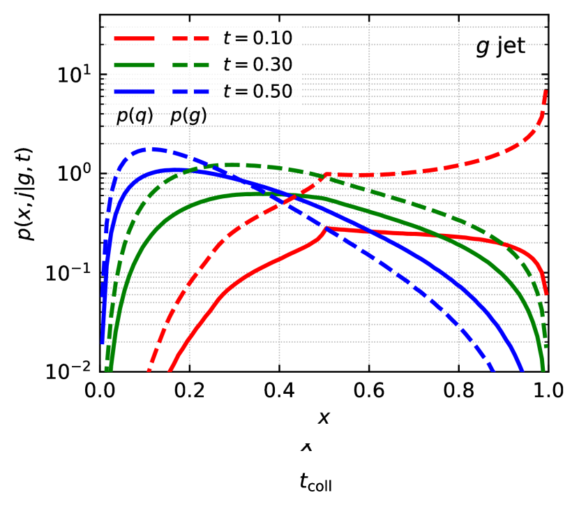
(b) gluon-initiated jet

Figure 1: Distributions $p(x,j|i,t_{\text{coll}})/f(j|i,t_{\text{coll}})$, with $f(j|i,t_{\text{coll}})$ the average fraction of partons of flavour $j$ after a time $t_{\text{coll}}$ starting from a flavour $i$ (cf. Eq. (16)), for different values of $t_{\text{coll}}$ as a function of $x$. The left (right) plot correspond to quark (gluon)-initiated jets. On both plots, the solid (dashed) lines correspond to a quark (gluon) leading parton.

In practice, an exact analytic calculation of $p(x,j|i,t_{\text{coll}})$ is not possible. It is however straightforward to obtain it numerically using the approach of Ref. Dasgupta:2014yra . A sample of the resulting distributions is shown in Fig. 1 for both quark-initiated and gluon-initiated jets. The distributions progressively shift towards smaller values of $x$ as expected.

From Eq. (12) one can also deduce a few analytic properties of $p(x,j|i,t_{\text{coll}})$. In particular, if one takes the $0^{\text{th}}$ and $1^{\text{st}}$ moments of (12) one obtains respectively an evolution equation for the average fraction of quarks and gluons and the average longitudinal momentum of the leading parton. We therefore define

$$f(j|i,t_{\text{coll}})=\int_{0}^{1}dx\,p(x,j|i,t_{\text{coll}})\quad\text{ and }\quad\bar{x}(j|i,t_{\text{coll}})=\frac{1}{f_{j}(i,t_{\text{coll}})}\int_{0}^{1}dx\,x\,p(x,j|i,t_{\text{coll}}).$$ (16)

For both $f$ and $f\bar{x}$ one can write a closed equation which admits a solution under the form of a (matrix) exponential. The solutions to these equations are given in Appendix A.

(a) Average partonic fraction.

(b) Average leading-parton momentum fraction.

Figure 2: Average parton fraction (left) and longitudinal momentum (right) as a function of the evolution time variable $t_{\text{coll}}$. The red (blue) curves correspond to a quark (gluon) initial parton. The solid (dashed) curves correspond to a quark (gluon) leading parton at time $t_{\text{coll}}$. The top axis shows the angle corresponding to $t_{\text{coll}}$ for a 2-TeV jet. The $t_{\text{coll}}$ axis extends significantly beyond the typical perturbative region so as to help illustrate the asymptotic trends.

Plots of $f(j|i,t)$ and $\bar{x}(j|i,t)$ are shown in Fig. 2 from which we can make several observations. First, as $t_{\text{coll}}\to\infty$, i.e. $\Delta\to 0$ (modulo Landau-pole complications), the quark and gluon fractions tend to constants that are independent of the initial flavour of the jet. From (49) one finds

$$f(q|\text{any},t_{\text{coll}}\to\infty)=\frac{s_{g}}{s_{q}+s_{g}},\qquad f(g|\text{any},t_{\text{coll}}\to\infty)=\frac{s_{q}}{s_{q}+s_{g}},$$ (17)

with $s_{q}=C_{F}(2\ln 2-\tfrac{5}{8})$ and $s_{g}=\tfrac{1}{3}n_{f}$. This means about 62.1% quarks and 37.9% gluons for $n_{f}=5$, in agreement with Fig. 2(a). Furthermore, for $t_{\text{coll}}\to 0$, we find

$$\lim_{t_{\text{coll}}\to 0}\frac{\bar{x}(g|q,t_{\text{coll}})}{t_{\text{coll}}}=\frac{w_{gq}}{s_{q}}\simeq 0.712,\qquad\lim_{t_{\text{coll}}\to 0}\frac{\bar{x}(q|g,t_{\text{coll}})}{t_{\text{coll}}}=\frac{w_{qg}}{s_{g}}\simeq 0.78125,$$ (18)

where the $w_{gq}$ and $w_{qg}$ coefficients are given analytically in Appendix A. The results in Eq. (18) correspond to the average harder-parton momentum fractions after a single $q\to qg$ splitting (with the gluon the harder particle) or a single $g\to q\bar{q}$ splitting. The numerical values are in agreement with Fig. 2(b).

3.3 Soft emissions at large or commensurate angles

The average primary Lund density is subject to several classes of effect associated with the non-trivial characteristics of soft radiation. At $\mathcal{O}\left(\alpha_{s}\right)$, when one goes beyond the collinear limit of Eq. (5) and considers radiation at angles $\Delta\sim 1$, soft gluon radiation is a coherent sum from all hard coloured partons in the event rather than just a single parton. At higher orders, two further effects arise: the presence of a first soft gluon contributes to the radiation of a subsequent second soft gluon at commensurate angles, and so forth for higher numbers of gluons, contributing effects similar to non-global logarithms; and in the presence of two or more gluons at commensurate angles, one must account for the way in which jet clustering determines whether a given gluon is classified as a primary or a secondary Lund emission. These two effects are present both for large and (perhaps more surprisingly) small $\Delta$.

In this section we will consider all of these effects, using the large-$N_{C}$ limit so as to retain simple colour algebra. After considering how we decompose events into separate colour flows, we shall in section 3.3.1 examine the impact of different colour flows on the large-angle part of the Lund plane at $\mathcal{O}\left(\alpha_{s}\right)$. Then in section 3.3.2 we shall consider the case of double (energy-ordered) soft gluon emission and derive the structure of the non-global and clustering logarithms in the small-angle limit at order $\alpha_{s}^{2}$. Finally in section 3.3.3 we will discuss how we generalise these results to resum all sources of single soft logarithms to all orders.

We start by recalling that in the large-$N_{C}$ limit, a given Born-level process can be expressed as a sum over several partonic channels where each of them is a weighted sum of different colour flows:

$$\rho_{\text{soft}}(\Delta,k_{t})=\sum_{c\in\text{channel}}\sum_{f\in\text{flows}}w_{c,f}\,\rho_{\text{soft}}^{(c,f)}(\Delta,k_{t}).$$ (19)

In this context, for each colour flow, one can view the Born-level process as a superposition of colour dipoles. Let us consider a dijet process with two incoming partons, $p_{1,2}$, and two outgoing partons, a jet parton $p_{j}$ and a recoiling parton $p_{r}$. The relative weights of the different partonic channels can be obtained from the $2\to 2$ squared matrix elements, e.g. using NLOJet++. Then, a $q_{\text{in}}q_{\text{in}}^{\prime}\to q_{\text{out}}q_{\text{out}}^{\prime}$ channel would have, in the large-$N_{c}$ limit, a single colour flow with weight $w=1$ corresponding to dipoles $[(q_{\text{in}}q_{\text{out}}^{\prime})+(q_{\text{in}}^{\prime}q_{\text{out}})]$. Similarly, a $g_{\text{in}}q_{\text{in}}\to g_{\text{out}}q_{\text{out}}$ channel would have two colour flows:

$$[(g_{\text{in}}g_{\text{out}})+(q_{\text{in}}g_{\text{out}})+(g_{\text{in}}q_{\text{out}})] \quad\text{ with weight }\quad\frac{s^{2}}{s^{2}+u^{2}},$$ (20a)

$$[(g_{\text{in}}g_{\text{out}})+(g_{\text{out}}q_{\text{out}})+(g_{\text{in}}q_{\text{in}})] \quad\text{ with weight }\quad\frac{u^{2}}{s^{2}+u^{2}},$$ (20b)

with $s,t,u$ the usual Mandelstam variables. The complete set of colour flows, dipole superpositions and weights can, for example, be deduced from Ref. Ellis:1986bv .

In the next sections, it will be helpful to separate $\rho_{\text{soft}}$ in different contributions according to the Born-level flavour of the jet:

$$\rho_{\text{soft}}(\Delta,k_{t})=\sum_{i\in\text{jet flavours}}f_{i}\>\rho_{\text{soft},i}(\Delta,k_{t}),$$ (21)

where $f_{i}$ denotes the relative fraction of quark and gluon jets. This separation in jet flavours can be straightforwardly obtained from (19).

We can expand $\rho_{\text{soft},i}$ as a series in $\alpha_{s}$:

$$\rho_{\text{soft},i}(\Delta,k_{t})=\sum_{n=1}^{\infty}\alpha_{s}^{n}\rho_{\text{soft},i}^{(n)}(\Delta,k_{t}).$$ (22)

In the first subsection below, we will show that $\rho_{\text{soft},i}^{(1)}$ deviates from (5) by corrections that are power-suppressed in $\Delta$. At our single-logarithmic accuracy, we have

$$\alpha_{s}^{n}\rho_{\text{soft},i}^{(n)}(\Delta,k_{t})\propto\alpha_{s}^{n}\ln^{n-1}\left(\frac{p_{\perp}\Delta}{k_{t}}\right).$$ (23)

These soft logarithms are either due to non-global configurations or to clustering logarithms associated with the Cambridge/Aachen reclustering used to construct the primary Lund-plane density. It is interesting to note that these clustering logarithms are present at arbitrarily small angles, which is somehow uncommon (though addressed also in Kang:2019prh ). We show how they appear at order $\alpha_{s}^{2}$ in section 3.3.2 and provide an all-order resummation in section 3.3.3.

3.3.1 Soft emissions at large angles: fixed-order study

For definiteness, let us consider the case of two incoming partons, $\ell_{1,2}$, and two outgoing partons, $\ell_{j,r}$, with the following kinematics:

$$\ell_{1}^{\mu} \equiv\frac{Q}{2}(0,0,1,1),$$ (24a)

$$\ell_{2}^{\mu} \equiv\frac{Q}{2}(0,0,-1,1),$$ (24b)

$$\ell_{j}^{\mu} \equiv p_{\perp}(1,0,\sinh y_{\text{jet}},\cosh y_{\text{jet}}),$$ (24c)

$$\ell_{r}^{\mu} \equiv p_{\perp}(-1,0,-\sinh y_{\text{jet}},\cosh y_{\text{jet}}),$$ (24d)

where $Q=p_{\perp}\cosh y_{\text{jet}}$ (with the jet transverse momentum $p_{\perp}\equiv\ell_{\perp}$, while its rapidity is equal to $y_{\text{jet}}$). We consider the jet of radius $R$ around $\ell_{j}$, while $\ell_{r}$ corresponds to the recoiling hard jet.

In the large-$N_{c}$ approximation we have to consider soft gluon emission from any of 6 possible colour dipoles: one incoming-incoming, two jet-incoming, two recoil-incoming and one jet-recoil. For a given dipole with legs $\ell_{a}$ and $\ell_{b}$, the contribution from a soft emission of momentum $k^{\mu}\equiv k_{\perp}(\cos\phi,\sin\phi,\sinh y,\cosh y)$ takes the form

$$\alpha_{s}\rho_{\text{soft,$ab$}}^{(1)}(\Delta,k_{t})=\int_{0}^{p_{\perp}}\!k_{\perp}dk_{\perp}\!\int dy\int_{0}^{2\pi}\frac{d\phi}{2\pi}\frac{\alpha_{s}N_{c}}{2\pi}\frac{\ell_{a}\cdot\ell_{b}}{(\ell_{a}\cdot k)(k\cdot\ell_{b})}\,\Delta\delta(\Delta-\Delta R)\,k_{t}\delta(k_{t}-k_{\perp}\Delta R),$$ (25)

with $\Delta R=\sqrt{(y-y_{\text{jet}})^{2}+\phi^{2}}$. For each dipole configuration, we can set $y=y_{\text{jet}}+\Delta R\cos\psi$ and $\phi=\Delta R\sin\psi$. The $k_{\perp}$ and $\Delta R$ integrations can then be evaluated trivially, leaving the integration over $\psi$. This integration usually cannot be computed exactly so we instead perform a series expansion in $\Delta^{2}$:

$$\alpha_{s}\rho_{\text{soft},12}^{(1)} =\frac{\alpha_{s}N_{c}}{\pi}\Delta^{2},$$ (26a)

$$\alpha_{s}\rho_{\text{soft},1j}^{(1)} =\frac{\alpha_{s}N_{c}}{\pi}\left[1+\frac{\Delta^{2}}{4}+\frac{\Delta^{4}}{144}+{\cal{O}}(\Delta^{8})\right],$$ (26b)

$$\alpha_{s}\rho_{\text{soft},jr}^{(1)} =\frac{\alpha_{s}N_{c}}{\pi}\left[1+\frac{\tanh^{2}y_{\text{jet}}}{4}\Delta^{2}+\frac{(\cosh^{2}y_{\text{jet}}-3)^{2}}{144\cosh^{4}y_{\text{jet}}}\Delta^{4}+\frac{\tanh^{2}y_{\text{jet}}}{64\cosh^{4}y_{\text{jet}}}\Delta^{6}+{\cal{O}}(\Delta^{8})\right],$$ (26c)

$$\alpha_{s}\rho_{\text{soft},1r}^{(1)} =\frac{\alpha_{s}N_{c}}{\pi}\left[\frac{e^{2y_{\text{jet}}}}{4\cosh^{2}y_{\text{jet}}}\Delta^{2}+\frac{1}{16\cosh^{4}y_{\text{jet}}}\Delta^{4}+\frac{\tanh^{2}y_{\text{jet}}}{64\cosh^{4}y_{\text{jet}}}\Delta^{6}+{\cal{O}}(\Delta^{8})\right],$$ (26d)

where additionally $\rho_{\text{soft},2j}^{(1)}=\rho_{\text{soft},1j}^{(1)}$ and $\rho_{\text{soft},2r}^{(1)}$ is obtained from $\rho_{\text{soft},1r}^{(1)}$ via the replacement $y_{\text{jet}}\to-y_{\text{jet}}$.

In the collinear limit, $\Delta\ll 1$, $\rho_{\text{soft},2j}^{(1)}$, $\rho_{\text{soft},1j}^{(1)}$ and $\rho_{\text{soft},jr}^{(1)}$ all tend to a constant, with corrections taking the form of power corrections in $\Delta^{2}$, as expected. The other dipoles are suppressed by a factor $\Delta^{2}$.

While running-coupling and collinear flavour-changing effects only depend on the flavour of the jet, the corrections due to soft emissions at large angles involve the structure of the whole event. The relative weight of each dipole depends on the channel and colour flow under consideration, cf. (19).

3.3.2 Soft emissions and Cambridge/Aachen clustering: fixed-order study

Say we want to extend the calculation from section 3.3.1 to order $\alpha_{s}^{2}$. The same calculation as above would have to be repeated with two soft emissions, $k_{1}$ and $k_{2}$, strongly ordered in energy ($k_{\perp 1}\gg k_{\perp 2}$). Measuring the emission $k_{2}$ and integrating out $k_{1}$ yields a contribution to the primary Lund plane density of the form

$$\alpha_{s}^{2}\rho_{\text{soft}}^{(2)}\propto\alpha_{s}^{2}\ln\frac{k_{t}}{p_{\perp}\Delta}.$$ (27)

In the limit $\Delta\to 0$ the prefactor is simple, and we calculate it here.

For concreteness, we illustrate the case of a quark-induced jet. We denote by $\theta_{i}$ the angle between $k_{i}$ and the quark and by $\theta_{12}$ the angle between $k_{1}$ and $k_{2}$ and work in a limit where all angles are small. In contrast to section 3.3.1, we now use a frame where the jet is perpendicular to the beam. In conjunction with the small-angle limit, this ensures that angles and rapidity-azimuth distances are equivalent, as are energies and transverse momenta (with respect to the beam).

Let us first consider three simple nested-collinear limits. When $\theta_{1}\gg\theta_{2}$, gluon $k_{2}$ is emitted with colour factor $C_{F}$ and declustered as a primary emission, i.e. the LO $2\alpha_{s}C_{R}/\pi$ emission intensity for gluon $k_{2}$ is unaffected by the presence of gluon $k_{1}$. The situation is similar when $\theta_{1}\ll\theta_{2}$. When $\theta_{12}\ll\theta_{1}$, gluon $k_{2}$ is emitted with colour factor $C_{A}$ and declustered as a secondary emission, i.e. on gluon $k_{1}$’s Lund leaf. The only non-trivial situation is when the angles $\theta_{1}$, $\theta_{2}$ and $\theta_{12}$ are commensurate, $\theta_{1}\sim\theta_{2}\sim\theta_{12}\ll 1$. In this region, one needs to account for the non-trivial matrix element for the emission of two gluons at commensurate angles and for the effects of the Cambridge/Aachen clustering used to construct the Lund plane. Together, these induce an $\mathcal{O}(\alpha_{s}^{2}\ln k_{t}/(p_{\perp}\Delta))$ correction to the $2\alpha_{s}C_{R}/\pi$ behaviour, where the logarithm is associated with the integral over the transverse momentum of gluon $k_{1}$.

This contribution to the primary Lund density for a quark-induced jet can be written

$$\alpha_{s}^{2}\rho_{\text{soft}}^{(2)}= \left(\frac{\alpha_{s}}{\pi^{2}}\right)^{2}\int_{0}^{p_{\perp}}\frac{dk_{\perp 1}}{k_{\perp 1}}\int_{0}^{k_{\perp 1}}\frac{dk_{\perp 2}}{k_{\perp 2}}\int d^{2}\theta_{1}\frac{C_{F}}{\theta_{1}^{2}}\int d^{2}\theta_{2}\;\Delta\,\delta(\Delta-\theta_{2})\,k_{t}\,\delta(k_{t}-k_{\perp 2}\Delta)$$

$$\left\{\left[\left(C_{F}-\frac{C_{A}}{2}\right)\frac{1}{\theta_{2}^{2}}+\frac{C_{A}}{2}\frac{1}{\theta_{12}^{2}}+\frac{C_{A}}{2}\frac{\theta_{1}^{2}}{\theta_{2}^{2}\theta_{12}^{2}}\right]\left[1-\Theta(\theta_{12}<\theta_{1})\Theta(\theta_{12}<\theta_{2})\right]-\frac{C_{F}}{\theta_{2}^{2}}\right\},$$ (28)

where $k_{\perp i}$ is the transverse momentum of $k_{i}$ relative to the beam. In this expression the first (second) term of the curly bracket corresponds to a real (virtual) emission $k_{1}$. For the real emission, we have two factors: the first square bracket corresponds to the matrix element for the emission of the soft gluon $k_{2}$ and the second square bracket imposes that the gluon $k_{2}$ is reconstructed as a primary emission, i.e. is not clustered with the emission $k_{1}$.

Eq. (3.3.2) genuinely encodes clustering effects. If we first consider the $C_{F}^{2}$ contribution, naively associated with two emissions from the hard quark, the virtual term partially cancels the real contribution, leaving a negative contribution with a factor $\Theta(\theta_{12}<\theta_{1})\Theta(\theta_{12}<\theta_{2})$, i.e. where emission $k_{2}$ clusters with emission $k_{1}$. Obviously, this contribution disappears in the collinear limit $\theta_{2}\ll\theta_{1},\theta_{12}$ as expected. Focusing now on the $C_{F}C_{A}$ term, naively associated with secondary $k_{2}$ emission, the only contribution comes from the situation where the emission is not clustered with its emitter, $k_{1}$, which vanishes in the collinear limit $\theta_{21}\ll\theta_{1}$.

The $k_{\perp 1}$ integration in Eq. (3.3.2) has a logarithmic enhancement from strong energy ordering $k_{\perp 2}\ll k_{\perp 1}\ll p_{\perp}$, leading to a contribution proportional to $\alpha_{s}^{2}\ln\frac{k_{t}}{p_{\perp}\Delta}$, as anticipated in Eq. (27), and no collinear divergence. The integrand is suppressed in the limits $\theta_{1}\to 0$ and $\theta_{1}\to\infty$ and only receives a contribution from $\theta_{1}\sim\theta_{2}$.

The integration over $k_{\perp 1}$, $k_{\perp 2}$, $\theta_{2}$ and one of the azimuthal angles ($\varphi_{1}$ or $\varphi_{2}$) can be trivially performed, leaving an integration over $\theta_{1}$ and an azimuthal angle $\varphi$. One finds

$$\alpha_{s}^{2}\rho_{\text{soft}}^{(2)}=0.323066\,\left(\frac{2\alpha_{s}}{\pi}\right)^{2}C_{F}(C_{F}-C_{A})\ln\frac{k_{t}}{p_{\perp}\Delta}\qquad\qquad\text{[quark]}.$$ (29)

The calculation for a gluon jet can be obtained by replacing $C_{F}\to C_{A}$ in Eq. (3.3.2). That replacement carries through directly to Eq. (29), giving

$$\alpha_{s}^{2}\rho_{\text{soft}}^{(2)}=0\qquad\qquad\text{[gluon]}.$$ (30)

Thus for a purely gluonic theory, the energy-ordered double-soft emission pattern and the C/A clustering combine in such a way that there is no $\alpha_{s}^{2}\ln k_{t}/(p_{\perp}\Delta)$ correction to the Lund density when $\Delta$ is small.

The above results are valid at small angles. Two additional classes of effect arise at large angles. Firstly, the clustering effects become sensitive to the coherent structure of the radiation from the complete hard event. This relates to the discussion in section 3.3.1. Secondly, if one identifies the jet with the anti-$k_{t}$ algorithm and reclusters its constituents with the C/A algorithm, there is an interplay between the two clusterings. This leads to another source of logarithmic enhancement

$$\alpha_{s}^{n}\ln^{m}\left(\frac{p_{\perp}R}{k_{t}}\right)\ln^{p}\left(\frac{R}{R-\Delta}\right),\qquad\text{with }m\leq n-1,\;p\leq n-1.$$ (31)

The $\ln(\frac{R}{R-\Delta})$ structure appears when a first emission, close to but outside the anti-$k_{t}$ jet boundary, splits collinearly such that one of its offspring is inside the boundary. The all-order resummation of these boundary logarithms is beyond the scope of this paper. They are however briefly discussed in Appendix B. Note that if the original jet is identified with the C/A algorithm, these boundary logarithms are absent.

3.3.3 Soft emissions: all-order treatment

The treatment of soft single logarithms to all orders requires us to consider configurations with arbitrarily many energy-ordered gluons at commensurate angles Dasgupta:2001sh , for which analytic approaches exist only in specific limits Banfi:2002hw . The technique we adopt is similar to that originally proposed for the resummation of non-global logarithms in Dasgupta:2001sh and the related clustering logarithms Appleby:2003sj ; Banfi:2005gj . We rely on a large-$N_{C}$ approximation (with subleading colour corrections up to order $\alpha_{s}^{2}$ in the collinear limit). Techniques that exist to resum non-global logarithms at full $N_{C}$ are so far applicable only for a limited set of observables Hatta:2013iba ; Hagiwara:2015bia .

Compared to the typical treatment of non-global and clustering logarithms we have one extra difficulty and one simplification. The difficulty has the following origin. Since non-global logarithms stem from emissions at commensurate angles one can usually impose an angular cut-off at an angle $\theta_{\text{min}}$ that is small compared to the physical angle one probes ($\pi/2$, a jet radius, the rapidity width of a slice, …). This helps limit the particle multiplicity and associated computational cost of the calculations. In the case of the primary Lund plane, we instead have to probe a large range of angles, meaning that potential angular cut-offs have to be taken small/large enough to cover this extended phase-space, resulting in increased computational demands. The simplification relative to normal non-global logarithm calculations relates to the fact that the Lund plane density doesn’t involve any Sudakov suppression (unlike say a hemisphere mass). That Sudakov suppression, specifically the part associated with primary emissions, can lead to low computational efficiency unless dedicated subtraction techniques are applies. In the case of the Lund plane density one can simply generate all the emissions without separating primary emissions from the other ones.

The basic approach to simulating soft emissions is to directly order them in energy, as done in Dasgupta:2001sh . In this case we just need to generate the full angular structure of the emissions and only retain their energy ordering. If gluon $k_{j}$ is emitted after $k_{i}$, then it has a much smaller energy. In this case clustering with the anti-$k_{t}$ algorithm is equivalent to keeping the particles in a radius $R$ around the hard parton. For C/A clustering, all the necessary distances are available from the angular structure of the event and the recombination of two particles is equivalent to replacing them with the harder one.

For our ultimate primary Lund plane predictions, we want to focus on the phase-space above a certain $k_{t}$ cut, below which the non-perturbative effects dominate. For a given minimum relative transverse momentum $k_{t,\text{min}}$ the minimum accessible angle is $\Delta_{\text{min}}=k_{t,\text{min}}/p_{\perp}$. We therefore have to take an angular cut-off for the event simulations that is sufficiently smaller that $\Delta_{\text{min}}$. If we generate emissions down to an energy $E_{\text{min}}$, many of these emissions will have a $k_{t}$ much smaller than $k_{t,\text{min}}$. For example for $\Delta=\Delta_{\text{min}}$, emissions would be generated down to $k_{t}=E_{\text{min}}\Delta_{\text{min}}\ll k_{t,\text{min}}$. This is not a problem per se, except for the fact that this approach generates many more emissions than absolutely necessary, which ends up being computationally challenging.

For this reason, we have adopted a different approach, more traditional in parton-shower event generators, namely we generate the emissions ordered in $k_{t}$. Say we work with a fixed coupling. The event is described as a collection of dipoles, each with a hard scale corresponding to their invariant mass $Q$. For the initial condition, we decompose the Born-level event as a sum over all possible dipole configurations. At any given stage of the event generation, corresponding to a given scale $k_{t}=k_{ti}$, we should be able to generate the next emission at a scale $k_{t,i+1}<k_{ti}$. If a dipole $(p_{1},p_{2})$ of invariant mass $Q_{12}$ splits, this is done by first generating $k_{t,i+1}$ according to the following Sudakov factor (which includes collinear radiation at each end of the dipole):

$$\exp\left[-\int_{\ln k_{t,i+1}}^{\ln k_{ti}}d\ln q_{t}\int_{\ln\ell_{t}/Q_{12}}^{\ln Q_{12}/\ell_{t}}d\eta\frac{2\alpha_{s}N_{c}}{\pi}\right]=\exp\left[-\frac{\alpha_{s}N_{c}}{\pi}\ln\frac{k_{ti}}{k_{t,i+1}}\ln\frac{Q_{12}^{2}}{k_{ti}\,k_{t,i+1}}\right].$$ (32)

One then decides the rapidity $\eta$ of the emission, uniformly distributed between $\ln k_{t,i+1}/Q_{12}$ and $\ln Q_{12}/k_{t,i+1}$ as well as an azimuthal angle $\phi$. The 4-momentum of the new emission is thus reconstructed as

$$k_{i+1}^{\mu}=\xi_{1}p_{1}^{\mu}+\xi_{2}p_{2}^{\mu}+k_{t,i+1}^{\mu}$$ (33)

with

$$\xi_{1}=\frac{k_{t.i+1}}{Q_{12}}e^{\eta},\qquad\xi_{2}=\frac{k_{t.i+1}}{Q_{12}}e^{-\eta},\qquad k_{t,i+1}^{\mu}=k_{t.i+1}(\cos\phi\,n_{1}^{\mu}+\sin\phi\,n_{2}^{\mu})$$ (34)

and $n_{1,2}$ two unit vectors orthogonal to $p_{1}$ and $p_{2}$.

Note that when a dipole $(p_{1},p_{2})$ splits into two new dipoles $(p_{1},k_{i+1})$, $(k_{i+1},p_{2})$, the energy scales of the two new dipoles can be straightforwardly obtained using

$$Q_{1k}^{2} =(p_{1}+k_{i+1})^{2}=\xi_{2}\,Q_{12}^{2}=Q_{12}\,k_{t,i+1}\,e^{-\eta},$$ (35)

$$Q_{k2}^{2} =(p_{2}+k_{i+1})^{2}=\xi_{1}\,Q_{12}^{2}=Q_{12}\,k_{t,i+1}\,e^{+\eta}$$ (36)

In order to reduce the inclusion of uncontrolled corrections beyond our intended resummation of single logarithms, we can perform another simplification. Recall that we are aiming to resum the energy logarithms due to clustering effects. Instead of computing the energy of each particle explicitly from its 4-momentum, we can directly project this momentum along the direction of the initial dipole. Let us denote by $(p,\bar{p})$ the hard-scattering momenta of a given initial colour dipole. For each emission, we want to find the contributions $z$ and $\bar{z}$ of its momentum fractions along the $p$ and $\bar{p}$ directions respectively. For the emission of a new particle $k$ from a $(p_{1},p_{2})$ dipole, we have

$$p_{1}^{\mu} =z_{1}p^{\mu}+\bar{z}_{1}\bar{p}^{\mu}+p_{t,1}^{\mu}$$ (37)

$$p_{2}^{\mu} =z_{2}p^{\mu}+\bar{z}_{2}\bar{p}^{\mu}+p_{t,2}^{\mu}$$ (38)

The new emission $k$ therefore has a projection $z_{k}$, $\bar{z}_{k}$ along the $p$, $\bar{p}$ directions given by

$$z_{k} =\xi_{1}z_{1}+\xi_{2}z_{2}\approx\frac{k_{t}}{Q_{12}}\max(z_{1}e^{\eta},z_{2}e^{-\eta}),$$ (39)

$$\bar{z}_{k} =\xi_{1}\bar{z}_{1}+\xi_{2}\bar{z}_{2}\approx\frac{k_{t}}{Q_{12}}\max(\bar{z}_{1}e^{\eta},\bar{z}_{2}e^{-\eta}),$$ (40)

where we have used Eq. (34) and replaced the sum over the two contributions by its maximum at our accuracy.

Iterating the above procedure for emissions ordered in $k_{t}$ produces an event where each particle has a 4-momentum as well as longitudinal fractions $z$ and $\bar{z}$ along their initial $(p,\bar{p})$ dipole. To reconstruct the primary Lund plane density we then proceed as follows: the anti-$k_{t}$ jet of radius $R$ is made of all the emissions within a radius $R$ of an initial hard parton. These particles can then be clustered using the C/A jet algorithm. This clustering uses the exact 4-momenta of the jets and a winner-takes-all-like Larkoski:2014uqa recombination scheme where the recombined particle is taken as the one of the two recombining particles with the largest [.1pt]$z$ ( - ) momentum along the jet direction. When we reconstruct the primary Lund plane density, the $\Delta$ coordinate is again taken from the exact angular kinematics, the $z$ variable from the event [.1pt]$z$ ( - ) and hence $k_{t}$ is obtained as $p_{t,\text{hard}}z\Delta$ with $p_{t,\text{hard}}$ the jet transverse momentum (w.r.t. the colliding beams) of the initial hard parton.

The above discussion is strictly speaking valid only in a fixed-coupling approximation. To account for running-coupling effects, we use the following procedure. For given Born-level kinematics (see e.g. (24)) and a given colour flow corresponding to a given initial set of dipoles, we generate a Monte Carlo event using a fixed $\alpha_{s}$. Following the procedure outlined in the previous paragraph we obtain the coordinates $\Delta$ and $z$ of the primary Lund declusterings. From the $z$ coordinate, we then determine an emission “time” $t_{\text{soft},\text{fc}}$ defined as $t_{\text{soft},\text{fc}}=\alpha_{s}\ln 1/z$. This procedure yields a resummed density $\rho_{\text{soft}}(\Delta,t_{\text{soft,fc}})$. To include running-coupling corrections at a given $k_{t}$ and $\Delta$, we simply use $\rho_{\text{soft}}(\Delta,t_{\text{soft}})$ with a $t_{\text{soft}}$ defined to include running-coupling effects:

$$\rho_{\text{soft}}\big{(}\Delta,t_{\text{soft}}(k_{t},p_{\perp}\Delta;\mu)\big{)},$$ (41)

with (cf. Eq. (10))

$$t_{\text{soft}}(k_{t},p_{\perp}\Delta;\mu)=\int_{k_{t}}^{p_{\perp}\Delta}\frac{dq_{t1}}{q_{t1}}\frac{\alpha_{s}(q_{t1})}{\pi}\equiv I_{\alpha}(k_{t},p_{\perp}\Delta;\mu).$$ (42)

Additionally, this approach can be straightforwardly extended to generate results at fixed-order. This will be useful to compare to the results derived in section 3.3.1 and 3.3.2 as well as for matching with exact fixed-order results in section 4.

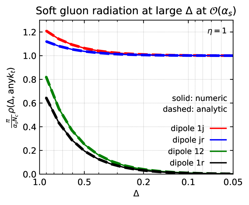
(a) Effects of soft gluon radiation at large angles for different dipole configurations (including or not the jet).

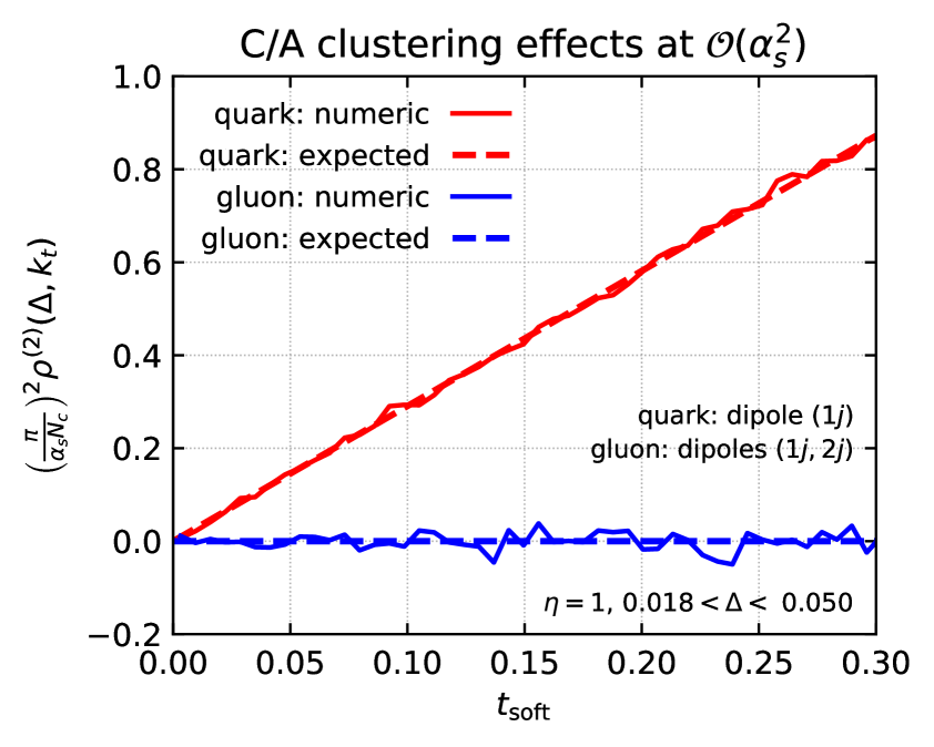
(b) Effects of Cambridge/Aachen clustering at order $\alpha_{s}^{2}$ in the collinear limit. Results are shown for two dipole configurations corresponding to a quark and gluon jet respectively.

Figure 3: Comparisons at fixed order between our numerical results for soft gluon radiation (solid lines) and analytic predictions from sections 3.3.1 and 3.3.2 (dashed lines).

As a validation of our numerical approach, we first compare the output of the numerical approach to the analytic results for soft gluon radiation at fixed order. The predictions for soft radiation at large angle at ${\cal{O}}(\alpha_{s})$, obtained in section 3.3.1, are compared to our numerical results in Fig. 3(a). The comparison is done assuming the large-$N_{c}$ limit and is independent of $\ln k_{t}$ (modulo the soft approximation of the kinematic constraint, $k_{t}/(p_{\perp}\Delta)\leq 1$). The figure shows excellent agreement with the analytic results from Eq. (26).

With Fig. 3(b), we study the numerical results for C/A clustering effects at ${\cal{O}}(\alpha_{s}^{2})$, Eqs. (29) and (30). For a gluon jet, we need to consider two dipoles. Since our calculation is done in the collinear limit, we have considered a range of small values of $\Delta$. The linear rise with $\ln z$, with the expected analytic coefficient, is clearly visible for quark jets, together with no effects at this order for gluon jets.

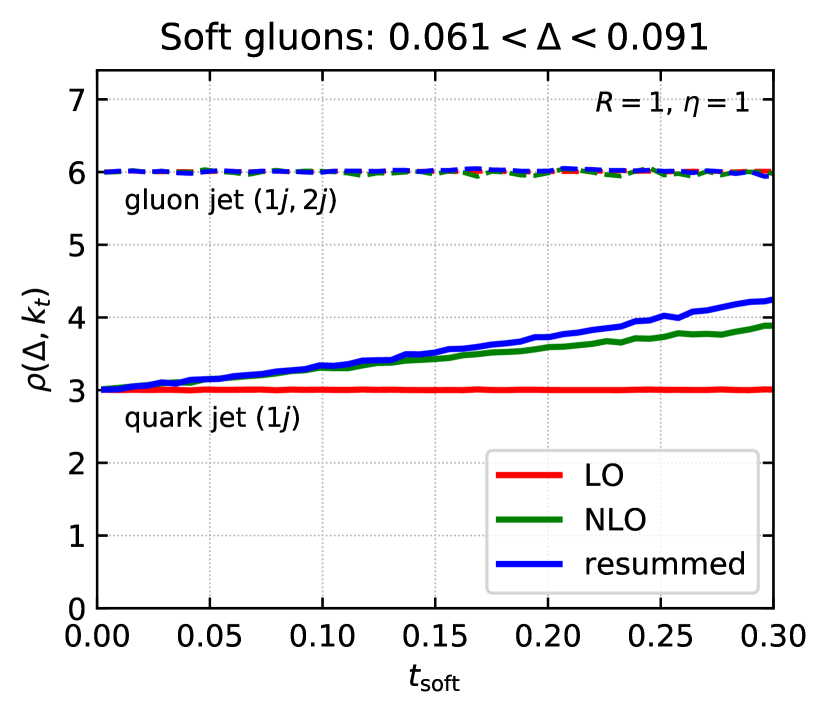
(a) Large angle, $0.449<\Delta<0.670$

(b) Small angle, $0.061<\Delta<0.091$

Figure 4: All-order resummation of logarithms from soft-gluon emissions. For both plots, we give the results for a quark configuration (solid lines) and a gluon configuration (dashed lines). LO (${\cal{O}}(\alpha_{s})$) and NLO (${\cal{O}}(\alpha_{s}^{2})$) results are shown for comparison. For the quark configuration we have used a $(1j)$ dipole connecting the incoming particle $\ell_{1}$ and the outgoing “jet” $\ell_{j}$, while for the gluon configuration, we have considered the superposition of 2 dipoles $(1j,2j)$, i.e. one dipole connecting the incoming $\ell_{1}$ with $\ell_{j}$ and a second dipole connecting the other incoming parton $\ell_{2}$ with $\ell_{j}$ (cf. (24)).

All-order results are shown in Fig. 4 for two different regions in angle. We see that apart from the region of very small $z$ (large $t_{\text{soft}}$), the resummation has a relatively small effect compared to the NLO result. A feature that is particularly intriguing is that in the collinear region, $\Delta\ll 1$, Fig. 4(b), the result appears to be independent of $t_{\text{soft}}$. Recall that for gluon jets, at order $\alpha_{s}^{2}$ the soft logarithmic term was identically zero for small $\Delta$, Eq. (30). Fig. 4(b) leads us to wonder whether the soft single logarithmic terms remain zero for gluon jets at all orders, or whether they are non-zero but simply too small to observe in our calculation. Note however that at large angles, Fig. 4(a), there is a clear $t_{\text{soft}}$ dependence both at $\alpha_{s}^{2}$ and beyond, i.e. the soft single logarithmic coefficients are non-zero.

3.4 Full resummed result

Our final resummed predictions include all the effects discussed in this section: the running of the strong coupling, collinear effects — flavour changes, splitting functions and the momentum of the leading parton — as well as soft-gluon emissions to all orders including large-angle contributions and clustering effects for emissions at commensurate angles:

$$\rho_{\text{resum}}(\Delta,k_{t}|p_{\perp})=\sum_{i,j=q,g}f_{i}(\mu_{F})\int_{0}^{1}dx\,p\big{(}x,j|i,t_{\text{coll}}(\Delta_{0},\Delta;\mu_{R})\big{)}\frac{\alpha_{s}(\xi_{K}k_{t})}{\pi}\\ \left(\frac{\mathcal{P}_{j}(z\equiv k_{t}/(xp_{\perp}\Delta))}{2C_{j}/z}\right)\rho_{\text{soft},j}\big{(}\Delta,t_{\text{soft}}(xp_{\perp}\Delta,\xi_{Z}k_{t};\mu_{R})\big{)}$$ (43)

In this expression, the factor $\alpha_{s}/\pi$ includes the 2-loop running coupling discussed in section 3.1. The scales $\mu_{R}=\xi_{R}p_{\perp}R$, $\mu_{F}=\xi_{F}p_{\perp}R$ and the factors $\xi_{K}$ and $\xi_{Z}$ probe the scale uncertainties and are discussed below. The factor $p(x,j|i,t_{\text{coll}})$ — computed numerically by solving Eq. (12) with an approach similar to Ref. Dasgupta:2014yra — encodes the probability for the leading parton to have a momentum fraction $x$ and a flavour $j$, starting from a jet of flavour $i$ (with initial fraction $f_{i}$) computed in the collinear limit as in section 3.2. Similarly, the factor $z\mathcal{P}_{j}/(2C_{j})$ accounts for the collinear structure associated with an observed Lund-plane emission at finite $z$ (cf. e.g. Eq. (15)). Finally, the factor $\rho_{\text{soft}}$ resums the soft logarithms at large angles as well as C/A clustering logarithms, as described in section 3.3.3. In practice, $\rho_{\text{soft}}$ depends on the full colour structure of an event. We have computed it by interfacing Born-level events obtained with the NLOJet++ program to the numerical code from section 3.3.3. Each Born-level event is separated (at large-$N_{c}$) into different (weighted) dipole configurations. The result is binned as a function of $t_{\text{soft}}$, $\Delta$, and the jet $p_{\perp}$ and flavour. The different dipole configurations contributing to a given jet flavour are summed, as only the sum is needed to combine $\rho_{\text{soft}}$ with the collinear effects in writing (43).

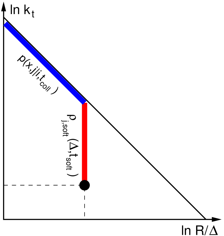
Figure 5: Schematic representation of Eq. (43) where the density at a point $(\Delta,k_{t})$ in the Lund plane is obtained by first resumming collinear effects at angles larger than $\Delta$ and then soft gluons (at commensurate angles) down to a scale $k_{t}$.

The structure of Eq. (43) is illustrated in Fig. 5, which shows that to obtain the density at a point $(\Delta,k_{t})$ in the Lund plane (the black dot), one first resums collinear effects down to the angle $\Delta$ (the solid blue line) then resums the soft emissions at commensurate angles between $xp_{\perp}\Delta$ and $k_{t}$ (the solid red line). In particular, one sees that at large angles, where the details of the dipole configuration matter, collinear effects can be neglected in (43) and the sum over dipole configurations can be performed trivially. At small angles, the clustering logarithms resummed in $\rho_{\text{soft}}$ depend only on the jet flavour.

Our results for the resummation of the soft gluons are strictly-speaking obtained in the large-$N_{c}$ limit. It is however possible to restore the full-$N_{c}$ behaviour up to and including $\mathcal{O}(\alpha_{s}^{2})$ in the collinear limit, i.e. in the limits that have been discussed in sections 3.3.1 and 3.3.2. First, we multiply the soft density for quark jets, $\rho_{\text{soft},q}$ by a factor $2C_{F}/C_{A}$ to guarantee the proper result from Section 3.3.1 at order $\alpha_{s}$. Then, we multiply $t_{\text{soft}}$ by $2(C_{A}-C_{F})/C_{A}$ for quark jets, to guarantee the proper expansion, Eq. (29), at order $\alpha_{s}^{2}$ in the collinear limit. At large angles the structure of subleading-$N_{C}$ corrections is more complicated, and we will rely on matching with fixed-order calculations to address these terms up to order $\alpha_{s}^{2}$.

To obtain our final predictions integrated over $p_{\perp}$, we have again used NLOJet++ to obtain the jet cross-section, the quark and gluon fractions $f_{q,g}$, the average jet $p_{\perp}$ and the average $\alpha_{s}(\mu_{R})$ (as well as $\rho_{\text{soft}}$) in a series of bins in $p_{\perp}$. The contribution of each bin is evaluated using (43) at the average $p_{\perp}$ in the bin and summed with weight proportional to the bin cross-section.

Compared to section 3.3.3, the definition of $t_{\text{soft}}$ from Eq. (42) has to be adjusted to ensure $t_{\text{soft}}\to 0$ when $k_{t}\to\tfrac{1}{2}xp_{\perp}\Delta$ (i.e. $z\to\tfrac{1}{2}$). This is simply done by writing

$$t_{\text{soft}}(\xi_{Z}k_{t},p_{\perp}\Delta;\mu)\equiv I_{\alpha}\left(\frac{\xi_{Z}xk_{t}}{x-(2-\xi_{Z})\frac{k_{t}}{p_{\perp}\Delta}},xp_{\perp}\Delta;\mu\right),$$ (44)

where we have introduced a parameter $\xi_{Z}$ that allows us, by a standard variation of $\xi_{Z}$ between $1/2$ and 2, to probe the uncertainties associated with the resummation of soft gluons. Similarly, we estimate the renormalisation ($\mu_{R}=\xi_{R}p_{\perp}R$) and factorisation ($\mu_{F}=\xi_{F}p_{\perp}R$) scale uncertainties using the 7-point rule Cacciari:2003fi around $\mu_{R}=\mu_{F}=p_{\perp}R$ ($\xi_{R}=\xi_{F}=1$). The factorisation scale only influences the Born-level spectrum and the quark/gluon fractions $f_{q,g}$. The choice of $\mu_{R}$ should also be reflected in the factor $\alpha_{s}/\pi$ in (43) as well as in the definition of $t_{\text{coll}}$ and $t_{\text{soft}}$, via the reference scale $\mu_{R}=\xi_{R}p_{\perp}R$ for $\alpha_{s}$ in (7). Additionally, the uncertainty of the choice of scale for the argument of $\alpha_{s}$ in (6) is taken into account by setting the scale to $\xi_{K}k_{t}$ and varying $\xi_{K}$ between $1/2$ and $2$. This is the dominant source of uncertainty in our calculation. The uncertainty on the collinear resummation could be estimated by varying $\Delta_{0}$ in (43). However, since the effect of the collinear resummation is small (see e.g. Figs. 6 and 7), we have neglected this and set $\Delta_{0}=R$. To be conservative, the final perturbative uncertainty is obtained by summing in quadrature the three individual sources of uncertainties: the 7-point variation of $\mu_{R}$ (or $\xi_{R}$) and $\mu_{F}$ (or $\xi_{F}$), the variation of $\xi_{K}$ and the variation of $\xi_{Z}$.

(a) large angles: $0.549<\Delta<0.670$

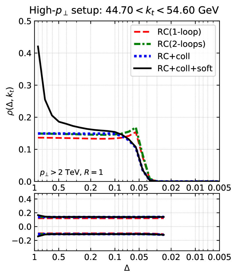
(b) small angles: $0.074<\Delta<0.091$

Figure 6: Slices of the resummed primary Lund-plane density $\rho_{\text{resum}}(\Delta,k_{t})$ at constant $\Delta$. The upper panels correspond to the density $\rho_{\text{resum}}(\Delta,k_{t})$ itself while the lower panels show the relative scale uncertainties $\tfrac{\delta\rho}{\rho}(\Delta,k_{t})$. We show results including different contributions: the dashed(red) line includes only 1-loop running, the (dash-dotted) green line includes 2-loop running-coupling corrections, the (dotted) blue lines adds the resummation of collinear effects (flavour changes and leading-parton momentum), and the solid black line is our full resummed result, including soft-gluon resummations as well.

(a) small $k_{t}$, $4.95<k_{t}<6.05$ GeV

(b) large $k_{t}$, $44.7<k_{t}<54.6$ GeV

Figure 7: Same as Fig. 6, now for slices of constant $k_{t}$.

We present some representative results obtained with Eq. (43) in Figs. 6 (for slices of the Lund plane in a narrow bin of $\Delta$) and 7 (for slices in a narrow bin of $k_{t}$). In each plot, we show results obtained using Eq. (6), i.e. just running-coupling effects, with 1-loop (red) and 2-loop (green) running. The blue curves then add collinear effects (i.e. Eq. (15)) and the black curves add soft-gluon emissions corresponding to our full resummed results from Eq. (43). The bottom panels of each plot show the corresponding scale uncertainties. These plots show that 2-loop running-coupling corrections are numerically similar in size to the resummation of the soft logarithms. Those soft-gluon effects are most significant at small $k_{t}$ and at large angle. It is worth noting though that their effect is also visible at large $k_{t}$ in Fig. 6(a). This is due to the power corrections in $\Delta^{2}$ starting at order $\mathcal{\alpha}_{s}$, as discussed in section 3.3.1.

Collinear effects are small except close to the $k_{t}=\tfrac{1}{2}p_{\perp}\Delta$ endpoint where the use of the full splitting function and the probability distribution for the momentum fraction of the leading parton have a clearly visible effect (see Fig. 7 in particular). Flavour-changing collinear effects are small but are still visible in Fig. 7(a), reflected in the difference between the green and blue lines for $\Delta\gtrsim 0.02$. In particular, as one goes to smaller values of $\Delta$, there is an increase in the fraction of jets whose leading parton is a gluon. This flavour-changing effect is modest in size, in part because the initial Born-level spectrum has a quark fraction of about $77.5\%$, relatively close to the asymptotic fraction of $62\%$ that is visible in Fig. 2(a) (cf. Eq. (17)).

The perturbative scale uncertainties are about 10% at large $k_{t}$, slowly growing to $\sim 15$% at $k_{t}\sim 20$ GeV and to $\sim 30$% at $k_{t}=2$ GeV (averaging the upper and lower uncertainties). They are dominated by the scale variation, $\xi_{K}$, in the argument of $\alpha_{s}$ with an additional small contribution from the variation of $\xi_{Z}$ at small $k_{t}$.

While all the above expressions are given for the primary Lund-plane density $\rho(\Delta,k_{t})$, they can almost straightforwardly be adapted to $\tilde{\rho}(\Delta,z)$, as measured e.g. by the ATLAS collaboration. Specifically, Eq. (43) becomes

$$\tilde{\rho}_{\text{resum}}(\Delta,z|p_{\perp})=\sum_{i,j=q,g}f_{i}\int_{0}^{1}dx\,p\big{(}x,j|i,t_{\text{coll}}(\Delta_{0},\Delta;p_{\perp}R)\big{)}\frac{\alpha_{s}(xzp_{\perp}\Delta)}{\pi}\\ \left(\frac{\mathcal{P}_{j}(z)}{2C_{j}/z}\right)\rho_{\text{soft},j}\big{(}\Delta,t_{\text{soft}}(xp_{\perp}\Delta,xzp_{\perp}\Delta;p_{\perp}R)\big{)}.$$ (45)

We just note that, while keeping $k_{t}$ large enough in Eq. (43) guarantees that we stay in the perturbative region, the integration over $x$ in (45) potentially extends to arbitrarily small $xzp_{\perp}\Delta$ momentum scales. This is regulated by our freezing of the running coupling at 1 GeV. In practice, this only affects the small values of $z$ in a region where the non-perturbative corrections dominate anyway.

In anticipation of the matching of our resummed predictions to exact fixed-order results for $\rho(\Delta,k_{t})$, we note that our all-order equations (43) and (45) can be expanded to fixed-order. For Eq. (43), at NLO we have

$$\alpha_{s}(k_{t}) =\alpha_{s}+2\alpha_{s}^{2}\beta_{0}\,\ln\frac{p_{\perp}R}{k_{t}},$$ (46a)

$$p(x,j|i,t_{\text{coll}}) =\delta_{ij}\delta(1-x)+\frac{\alpha_{s}}{\pi}\ln\frac{\Delta_{0}}{\Delta}\int dz\left[\mathcal{P}^{(R)}_{ji}(z)\delta(z-x)-\mathcal{P}^{(V)}_{ji}(z)\delta(1-x)\right],$$ (46b)

$$\rho_{\text{soft},j}\big{(}\Delta,t_{\text{soft}}\big{)} =\alpha_{s}\rho_{\text{soft},j}^{(1)}(\Delta,k_{t})+\alpha_{s}^{2}\rho_{\text{soft},j}^{(2)}(\Delta,k_{t})=\alpha_{s}\rho_{\text{soft},j}^{(1)}(\Delta)+\frac{\alpha_{s}^{2}}{\pi}\ln\frac{p_{\perp}\Delta}{k_{t}}\rho_{\text{soft},j}^{(2\text{-em})}(\Delta).$$ (46c)

with $\alpha_{s}\equiv\alpha_{s}(p_{\perp}R)$. We have explicitly written $\alpha_{s}^{2}\rho_{\text{soft}}^{(2)}(\Delta,k_{t})=\tfrac{\alpha_{s}^{2}}{\pi}\ln\tfrac{p_{\perp}\Delta}{k_{t}}\rho_{\text{soft}}^{(2\text{-em})}(\Delta)$, i.e. as a logarithm times a factor depending only on $\Delta$. The coefficients of the $\rho_{\text{soft}}$ expansion can be obtained, as for $\rho_{\text{soft}}$ itself, using the numerical approach from section 3.3.3 with a Born-level spectrum from NLOJet++. Inserting the elements of Eq. (46) into (43), we get a trivial LO contribution involving $\rho_{\text{soft},j}^{(1)}(\Delta)$. The NLO, i.e. $\mathcal{O}(\alpha_{s}^{2})$, result receives 3 contributions, one from each of the lines of Eq. (46). A similar fixed-order expansion can be obtained for $\tilde{\rho}(\Delta,z)$.

4 Matching with fixed-order

In order to get a full coverage of the primary Lund-plane density, including regions which are not dominated by large logarithms, it is useful to supplement our resummation with as many orders of the $\alpha_{s}$ series expansion of $\rho(\Delta,k_{t})$ as are known exactly.

In this paper we focus on dijet events, for which we can obtain the primary Lund-plane density using the NLOJet++ program,

$$\rho_{\text{fixed-order}}(\Delta,k_{t})=\alpha_{s}(p_{\perp}R)\,\rho^{(1)}(\Delta,k_{t})+\alpha_{s}^{2}(p_{\perp}R)\,\rho^{(2)}(\Delta,k_{t})+{\cal{O}}(\alpha_{s}^{3}).$$ (47)

The first (LO) and second (NLO) contributions are accessible using respectively LO and NLO 3-jet calculations Nagy:2003tz .

Compared to the all-order calculation discussed in section 3, the LO contribution includes the first-order soft gluon radiation at large angles. The NLO contribution includes the first non-trivial running-coupling, flavour-changing and clustering corrections. We have checked numerically that there was an agreement between NLOJet++ and our analytic calculations for the soft-and-collinear behaviour at $\mathcal{O}(\alpha_{s})$ and for the logarithmic dependence at $\mathcal{O}(\alpha_{s}^{2})$, although small deviations expected from our large-$N_{c}$ approximation — used to calculate dipole decompositions and soft logarithms beyond the collinear limit — are observed at large angles. We show some explicit examples in Appendix C.

Knowing both the all-order resummation and the exact fixed-order results, we obtain a matched prediction using

$$\rho(\Delta,k_{t})=\frac{\rho_{\text{resum}}(\Delta,k_{t})\,\rho_{\text{NLO}}(\Delta,k_{t})}{\rho_{\text{resum,NLO}}(\Delta,k_{t})},$$ (48)

where $\rho_{\text{resum,NLO}}$ is the expansion to ${\cal{O}}(\alpha_{s}^{2})$ of the resummed result (43). This expression is such that it reproduces the resummed calculation in the region where large logarithms are present, and the exact NLO result when expanded to second order in $\alpha_{s}$.

(a) large angles: $0.549<\Delta<0.670$

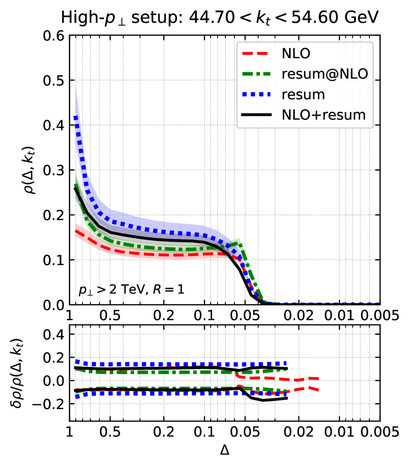
(b) small angles: $0.074<\Delta<0.091$

Figure 8: Slices of the primary Lund-plane density $\rho(\Delta,k_{t})$ at constant $\Delta$. The upper panels correspond to the density $\rho(\Delta,k_{t})$ itself, while the lower panels show the relative scale uncertainties $\tfrac{\delta\rho}{\rho}(\Delta,k_{t})$. We show results for the exact NLO calculation (red), the NLO expansion of the resummed results (green), the full resummed result (blue) and the NLO+resummation matched result (black).

Explicit examples of matched predictions, including different levels of approximations for the resummation, are presented in Fig. 8 for the $k_{t}$ dependence at fixed $\Delta$. First, we see that the exact NLO results (red) are close to what is obtained using the expansion of our resummed calculation (green). Next, the resummed result (blue) shows a strong enhancement at small $k_{t}$, primarily due to the running coupling, and to soft-gluon clustering effects. Finally, the matched result (black) smoothly interpolates between the fixed-order result at large angle and large $k_{t}$ and the resummed result at smaller angle or $k_{t}$.

The bands in the upper panel of Fig. 8 as well as the curves in the lower panel show our theoretical uncertainties. One of the striking features is that the matching with NLO reduces the uncertainties compared to the resummed result. This is valid across the whole kinematic range and especially visible at larger $k_{t}$. Final uncertainties after matching are $\sim 6\%$ at $k_{t}=200$ GeV, increasing to $\sim 12\%$ at 20 GeV and $\sim 30\%$ at 2 GeV.

5 Non-perturbative effects

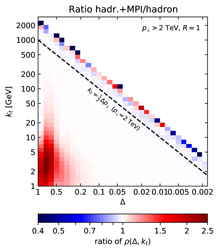
(a) Hadronisation corrections

(b) Underlying Event/MPI corrections

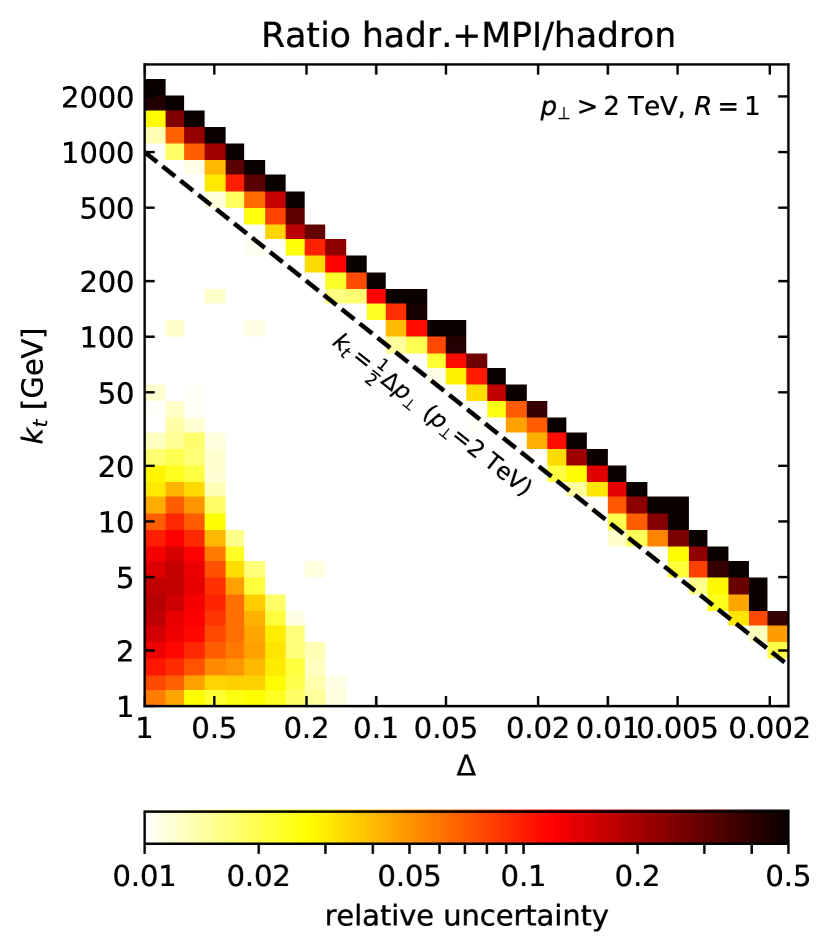
(c) Hadronisation uncertainties

(d) Underlying Event/MPI uncertainties

Figure 9: Non-perturbative corrections (top) and uncertainties (bottom). The diagonal dashed line corresponds to the kinematic limit, $k_{t}=\tfrac{1}{2}p_{\perp}\Delta$, for jets with $p_{\perp}=2$ TeV.

Before making our final predictions it is interesting to estimate non-perturbative corrections to the calculation we have provided so far. We do so using a Monte-Carlo approach. We have studied the primary Lund-plane density using 5 different Monte-Carlo generators/tunes: Pythia8 (v8.230) Sjostrand:2014zea with the Monash 2013 tune Skands:2014pea , tune 4C Corke:2010yf and the ATLAS 2014 tune ATL-PHYS-PUB-2014-021 (the variant with NNPDF 2.3 PDFs Carrazza:2013axa ), Herwig7.2.0 Corcella:2002jc ; Bellm:2015jjp ; Bellm:2019zci and Sherpa 2.2.8 Gleisberg:2008ta . For each generator/tune we first study the primary Lund-plane density at parton level. We can then switch to hadron level to study the effect of hadronisation, include multi-parton interactions (MPI) to study the effects of the Underlying Event, and examine the impact of using only charged tracks as done in the ATLAS measurement ATLAS:2019sol .

For the central value of the non-perturbative corrections, we take the average of the Monte-Carlo generators, excluding Herwig7. The reason behind this exclusion is that our perturbative results are in the same ballpark as parton-level results from Pythia8 and Sherpa but differ significantly from parton-level Herwig7 results (see Appendix D). We obtain the (upper and lower) uncertainties on the non-perturbative corrections from the envelope of the Lund-plane density ratios for the 5 Monte-Carlo generators/tunes. To remain conservative, we keep the Herwig7 results in our non-perturbative uncertainty estimates.

Our results are presented in Fig. 9, for our high-$p_{\perp}$ setup separately for hadronisation and Underlying Event corrections. It is clearly visible that hadronisation corrections become sizeable at low $k_{t}$, with a negative effect above $\sim 3$ GeV and a positive effect below. Their effect is almost invisible for $k_{t}\gtrsim 10{-}20$ GeV. Underlying-Event corrections are instead important (and positive) at low-to-moderate $k_{t}$ and large angles. The non-perturbative uncertainties — shown in Fig. 9(c) and 9(d) for hadronisation and the Underlying Event, respectively — are small, $\mathcal{O}(1{-}2)\%$, whenever the overall corrections are themselves small. At large $\Delta$, the non-perturbative corrections appear to have additional structure and enhanced uncertainties. This structure can be attributed to the interplay between the initial anti-$k_{t}$ clustering and the C/A re-clustering as already discussed in Dreyer:2018nbf and related boundary logarithms discussed in section 3.3.2 and Appendix B.

The diagonal dashed line in Fig. 9 corresponds to $k_{t}=\frac{1}{2}p_{\perp}\Delta$ for $p_{\perp}=2$ TeV. This is the kinematic limit for the lowest-energy selected jets. The Lund plane density quickly decreases above that line. The large fluctuations and uncertainties observed in Fig. 9 around the dotted line are a trace of the statistical fluctuations in our Monte Carlo samples.

6 Final predictions

(a) Lund-plane density $\rho(\Delta,k_{t})$

(b) Perturbative uncertainty

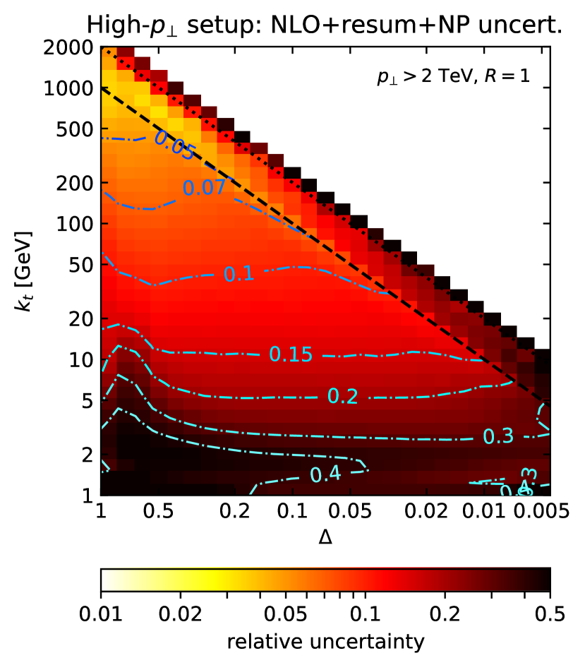
(c) Full uncertainty

Figure 10: Predictions for the primary Lund plane density for the high-$p_{\perp}$ setup (a) and associated perturbative (b) and full (c) uncertainties. Full uncertainties sum the perturbative and non-perturbative contributions in quadrature.

Our final predictions include both the matched perturbative predictions, discussed in section 4, multiplied by the non-perturbative corrections obtained in section 5.

We show in Fig. 10(a) the resulting two-dimensional average primary Lund-plane density $\rho(\Delta,k_{t})$, and in Figs. 10(b) and 10(c) the associated relative uncertainty at perturbative level and at the non-perturbative level respectively. Fig. 11 shows slices at fixed angle $\Delta$, which help to better visualise certain features. The density plot, Fig. 10(a), shows all the expected features: the gradual increase towards small $k_{t}$ due to the running of $\alpha_{s}$; the extra enhancement due to soft-gluon emissions, both at large angles and at small $k_{t}/\Delta$ (or equivalently $z$); the reduction close to the kinematic limit associated with the “energy loss” of the leading branch; and the increase at low $k_{t}$ and in the bottom-left corner of the Lund plane due to non-perturbative effects.

The uncertainties are dominated by the perturbative component for $k_{t}\gtrsim 3{-}5$ GeV, except at large angles where non-perturbative effects can have a sizeable impact up to $k_{t}\sim 10{-}20$ GeV. The total uncertainty is found to be about $20\%$ at $k_{t}\sim 5$ GeV (away from the large-angle region), and decreases to $5{-}7\%$ for $k_{t}$ in the $200{-}500$ GeV range. Relative to the LO+resum results, visible in Fig. 11, the inclusion of NLO corrections reduces the uncertainties mainly at high $k_{t}$. Even if the non-perturbative corrections have a negligible impact on the uncertainty above $\sim 3{-}5$ GeV ($10{-}20$ GeV) at small (large) $\Delta$, they result in a (small-but-visible) shift of the central value up to larger values of $k_{t}$.

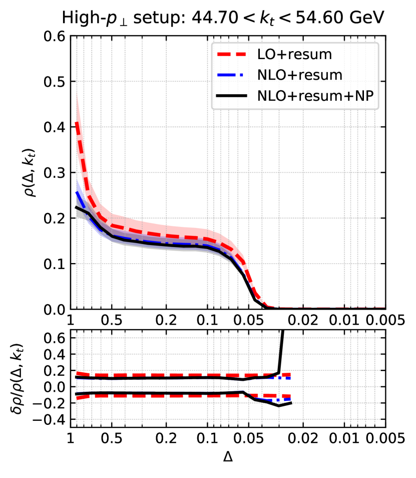
(a) large angles: $0.549<\Delta<0.670$

(b) small angles: $0.074<\Delta<0.091$

Figure 11: Slices of the primary Lund-plane density $\rho(\Delta,k_{t})$ at constant $\Delta$. The upper panels correspond to the density $\rho(\Delta,k_{t})$ itself while the lower panels show the relative scale uncertainties $\tfrac{\delta\rho}{\rho}(\Delta,k_{t})$. We show results for the matched result at LO (red) and NLO (blue), as well as NLO results including non-perturbative corrections (black).

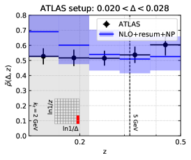
Figure 12: Comparison between our calculations and the ATLAS measurement from Ref. ATLAS:2019sol , for different bins of $\Delta$. The dashed vertical lines, corresponding to $z=\tfrac{k_{t}}{p_{\perp}\Delta}$ for $p_{\perp}=675$ GeV and several $k_{t}$ values, are meant to indicate the transverse scales one is typically sensitive to. The shaded grey bands indicate bins where the relative uncertainty on the non-perturbative corrections is larger than 10%. The shaded red regions indicate that our calculation is incomplete because of the missing resummation of the boundary logarithms.

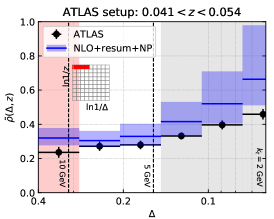
Figure 13: Same as Fig. 12 this time for slices at constant $\ln(1/z)$.

Finally, we discuss our analytic calculations supplemented with non-perturbative corrections for $\tilde{\rho}(\Delta,z)$, corresponding to the ATLAS setup. Besides the differences discussed in section 2, we follow the same strategy as for the high-$p_{\perp}$ setup: the resummed prediction is obtained using Eq. (45), matched to NLOJet++ fixed-order results using Eq. (48) and supplemented with non-perturbative corrections — this time correcting so as to correspond to a measurement performed using charged-tracks above 500 MeV — following the procedure outlined in section 5. Details of the non-perturbative corrections are given in Appendix E.

We compare our results to the ATLAS data from Ref. ATLAS:2019sol for slices in $\Delta$ in Fig. 12 and slices in $z$ in Fig. 13. The vertical dashed lines correspond to the $k_{t}$ scales estimated using $z=k_{t}/(p_{\perp}\Delta)$, i.e. assuming a jet at the lower $p_{\perp}$ cut of 675 GeV and a leading parton/subjet carrying a fraction $x=1$ of the initial jet transverse momentum. The shaded grey bands indicate regions where the uncertainty on the non-perturbative corrections is larger than 10%. Shaded red bands correspond to the regions sensitive to the boundary logarithms discussed in section 3.3.2. We recall that we have not resummed these terms, so our calculation should be considered incomplete in the red shaded regions. A rough estimate of their potential size is given in Appendix B.

For all unshaded bins in Figs. 12 and 13, we see agreement between our predictions and the data to within the experimental and theoretical uncertainties. Generally speaking, the theoretical uncertainties are larger than the experimental ones, though they are comparable at values of $z$ and $\Delta$ that correspond to large $k_{t}$ values. Recall that the theoretical uncertainties are to a large extent dominated by the choice of scale of $\alpha_{s}$ in the resummation and a higher-order resummation would therefore be beneficial to reduce the uncertainties.

If we consider the grey shaded regions, i.e. those where non-perturbative uncertainties are larger than $10\%$, the agreement between data and theory remains good to within the total uncertainties in most of the bins, almost all the way down to $2\,\text{GeV}$. In practice this agreement is facilitated by the non-perturbative blow-up of the uncertainties at low $k_{t}$ and our predictions’ central values are systematically above the data points. Recall, however, that our estimates of non-perturbative corrections rely on the assumption that the parton-level event-generator results are structurally similar to a full perturbative calculation. This assumption is questionable at low $k_{t}$: for example, a parton shower may contain a low-$k_{t}$ cut, with the phase-space below that $k_{t}$ value being filled up by hadronisation (there is a hint of this occurring in Appendix D, Fig. 16); in contrast our perturbative calculation has no such cut, and so the hadronisation contribution to that region, supplemented with our perturbative contribution, could effectively lead to double counting and so an overestimate relative to the data. In this respect it might be interesting to develop a more analytic understanding of expected hadronisation effects on the Lund plane density.

One region where there is clear disagreement between our predictions and the data is in the (red-shaded) largest angle bin $0.287<\Delta<0.400$. This disagreement is only mildly alleviated by our estimate of the potential size of boundary logarithms, cf. Fig. 14 in Appendix B. Several avenues could be of interest for further exploring this region, for example a full resummation of the boundary logarithms, or a measurement with jets whose original clustering was with the C/A algorithm (rather than anti-$k_{t}$), so as to remove these boundary logarithms altogether. Note also that this region is potentially sensitive to underlying-event effects, and if they are incompletely modelled in event generators, this could also contribute to the disagreement.

7 Conclusions and outlook

In this paper we have carried out the first calculation of all-order logarithmic contributions to the average primary Lund plane density. We have resummed three classes of single logarithmic terms: (i) running-coupling effects, which are relatively straightforward and the numerically dominant contribution over most of the Lund plane; (ii) soft effects, which involve large-angle contributions and clustering logarithms, both evaluated in the large-$N_{C}$ limit; and (iii) collinear effects at large momentum fractions, which include contributions that can change both the momentum and the flavour of the leading parton. We have also discovered a new class of logarithmic effects in jets that arise when reclustering an anti-$k_{t}$ jet’s constituents with the Cambridge/Aachen algorithm. The corresponding terms are relevant close to the large-angle boundary of the Lund plane. We defer their full single logarithmic resummation to future work.

For the purposes of making phenomenological predictions, we have matched our all-order, resummed, calculation to an exact (3-jet) calculation at next-to-leading order with the NLOJet++ program. We then supplemented the perturbative predictions with non-perturbative effects extracted from Monte Carlo simulations with Herwig, Pythia and Sherpa.

The theoretical uncertainty on our perturbative predictions ranges from $5{-}7\%$ at large $k_{t}$ to $\sim 20\%$ at $k_{t}\approx 5$ GeV. Hadronisation and underlying-event corrections are relevant below $20{-}30\,\text{GeV}$, but in most of the Lund plane dominate the overall uncertainty only below $k_{t}\sim 3{-}5$ GeV ($15\,\text{GeV}$ at large angles, where the underlying event is a significant contributor), cf. Figs. 10 and 11.

We have made our predictions for two variants of the Lund plane definition, one using angle and absolute transverse momentum (the default for most of this paper), and the other using angle and relative momentum fraction in a given branching. The latter corresponds to the choice made by the ATLAS collaboration in their recent pioneering unfolded measurement of the primary Lund plane density with charged tracks Aad:2020zcn . We have compared our results to the ATLAS data, including an additional non-perturbative correction to account for the use of charged tracks, and found good agreement in all regions where we have confidence in our predictions, i.e. the non-shaded regions of Figs. 12 and 13. This includes a broad swathe of the Lund plane, down to scales corresponding to transverse momenta of about $5\,\text{GeV}$.

Our work opens a series of questions that should be kept in mind for future work. First, it would be interesting to extend our calculation beyond single-logarithmic accuracy. We expect that this would give a considerable reduction in the uncertainty, notably from control over the effective scale to be used in the coupling. Such a calculation, however, remains challenging. Other effects like the subleading-logarithmic and subleading-$N_{c}$ corrections to the clustering logarithms, or NNLO fixed-order corrections (requiring a NNLO $pp\to 3$-jet calculation) would also be expected to bring significant improvements in certain specific regions of the Lund plane.

It would also be of interest to understand the resummation of the boundary logarithms that originate from the interplay between the initial anti-$k_{t}$ clustering and the C/A reclustering. Practically, however, these logarithms could be avoided by using the C/A algorithm for both the initial clustering and the reclustering. One observation that would also deserve better understanding is the apparent absence of any resummation effect from clustering logarithms in the soft-collinear part of the Lund plane for gluon-induced jets

Keeping the above theoretical limitations in mind (and possible future improvements), one might wish to investigate whether a measurement of the Lund plane density, which intrinsically covers a wide range of transverse-momentum scales, could be helpful to make an extraction of the strong coupling constant, $\alpha_{s}$, extending existing work on strong coupling determinations from soft-drop measurements Bendavid:2018nar ; Marzani:2019evv . In a similar spirit, one could perhaps extend the approach of Ref. Dokshitzer:1995zt to develop an analytic approach to non-perturbative corrections at small $k_{t}$ and potentially even use Lund-plane measurements to determine an effective coupling constant down to small transverse momenta.

Finally, it would be interesting to compare both analytical predictions and measurements of the primary Lund-plane density to recent efforts to develop parton showers with perturbative control beyond leading double logarithmic accuracy (e.g. Dasgupta:2020fwr ; Forshaw:2020wrq ) and leading colour (e.g. Forshaw:2019ver ; Nagy:2019pjp ).

Appendix A Analytic results for collinear resummation

In this Appendix we give the explicit analytic solutions for the average quark/gluon fractions $f(j|i,t_{\text{coll}})$ and momentum fraction $\bar{x}(j|i,t_{\text{coll}})$ defined in Eq. (16). We find

$$f(q|i,t) =\delta_{iq}-\frac{s_{q}\delta_{iq}-s_{g}\delta_{ig}}{s_{q}+s_{g}}\left(1-e^{-(s_{q}+s_{g})t}\right),$$ (49a)

$$f(g|i,t) =\delta_{ig}+\frac{s_{q}\delta_{iq}-s_{g}\delta_{ig}}{s_{q}+s_{g}}\left(1-e^{-(s_{q}+s_{g})t}\right),$$ (49b)

$$f\bar{x}(q|i,t) =e^{tw_{+}}\left\{\left[\cosh(t\tilde{w}_{+})+\frac{w_{-}}{\tilde{w}}\sinh(t\tilde{w})\right]\delta_{iq}+\frac{w_{qg}}{\tilde{w}}\sinh(t\tilde{w})\,\delta_{ig}\right\}$$ (49c)

$$f\bar{x}(g|i,t) =e^{tt_{+}}\left\{\left[\cosh(t\tilde{w}_{+})-\frac{w_{-}}{\tilde{w}}\sinh(t\tilde{w})\right]\delta_{ig}+\frac{t_{gq}}{\tilde{w}}\sinh(t\tilde{w})\,\delta_{iq}\right\},$$ (49d)

with

$$w_{\pm}=\frac{w_{qq}\pm w_{gg}}{2},\qquad\tilde{w}=\sqrt{w_{-}^{2}+w_{qg}w_{gq}}.$$ (50)

and

$$s_{q} =\int_{0}^{1}dz\,\left[{\cal{P}}_{qg}^{(R)}(z)-{\cal{P}}_{qg}^{(V)}(z)\right]=C_{F}\left(2\ln 2-\frac{5}{8}\right),$$ (51a)

$$s_{g} =\int_{0}^{1}dz\,\left[{\cal{P}}_{gq}^{(R)}(z)-{\cal{P}}_{gq}^{(V)}(z)\right]=\frac{2n_{f}T_{R}}{3},$$ (51b)

$$w_{qq} =\int_{0}^{1}dz\,\left[z{\cal{P}}_{qq}^{(R)}(z)-{\cal{P}}_{qq}^{(V)}(z)\right]=-C_{F}\left(2\,\ln 2+\frac{1}{6}\right),$$ (51c)

$$w_{qg} =\int_{0}^{1}dz\,\left[z{\cal{P}}_{qg}^{(R)}(z)-{\cal{P}}_{qg}^{(V)}(z)\right]=\frac{25}{48}n_{f}T_{R},$$ (51d)

$$w_{gq} =\int_{0}^{1}dz\,\left[z{\cal{P}}_{gq}^{(R)}(z)-{\cal{P}}_{gq}^{(V)}(z)\right]=\frac{11}{24}C_{F},$$ (51e)

$$w_{gg} =\int_{0}^{1}dz\,\left[z{\cal{P}}_{gg}^{(R)}(z)-{\cal{P}}_{gg}^{(V)}(z)\right]=-\frac{2}{3}n_{f}T_{R}-C_{A}\left(2\,\ln 2-\frac{43}{96}\right).$$ (51f)

Note that the coefficients $s_{q}$ and $s_{g}$ are in agreement with the flavour-changing effects calculated in Dasgupta:2014yra .

Appendix B Boundary logarithms for $\Delta\sim R$

In this Appendix, we show how new logarithms of $R-\Delta$ arise from secondary emissions at order $\alpha_{s}^{2}$. We show that these logarithms are a consequence of the interplay between the initial anti-$k_{t}$ clustering used to obtain the initial jets and the C/A clustering used to construct the primary Lund plane.

Say we start from a dipole $(\ell_{i},\ell_{j})$ and have 2 emissions, $k_{1}$ and $k_{2}$, strongly ordered in transverse momentum as discussed in Section 3.3.2. Emission $1$ (real or virtual) is integrated over and the softer emission 2 (real) is measured as a contributing to $\rho^{(2)}_{\text{soft}}(k_{t},\Delta)$.

We denote by $(k|ij)$ the geometrical pattern associated with the radiation of gluon $k$ from the dipole $(\ell_{i},\ell_{j})$ (i.e. the transverse momenta with respect to the beam are factored out). We also denote by $R_{i}$ the distance of $i$ to the jet axis (in rapidity-azimuth) and $R_{ij}$ the distance between $i$ and $j$. For a parton with Casimir $C_{R}$, we have

$$\alpha_{s}^{2}\rho^{(2)}_{\text{soft}}=\left(\frac{\alpha_{s}}{\pi}\right)^{2} \int_{0}^{p_{\perp}}\frac{dk_{\perp 1}}{k_{\perp 1}}\int_{0}^{k_{\perp 1}}\frac{dk_{\perp 2}}{k_{\perp 2}}\int dy_{1}dy_{2}\int_{0}^{2\pi}\frac{d\phi_{1}}{2\pi}\frac{d\phi_{2}}{2\pi}\Delta\delta(\Delta-R_{2})\,k_{t}\delta(k_{t}-k_{\perp 2}\Delta)$$

$$C_{R}(1|ij)\Bigg{\{}\left[\frac{C_{A}}{2}(2|i1)+\frac{C_{A}}{2}(2|1j)+\left(C_{R}-\frac{C_{A}}{2}\right)(2|ij)\right]$$ (52)

$$\phantom{C_{R}(1ij)}\left[\Theta(R_{1}>R)+\Theta(R_{1}<R)\Theta(R_{1}<R_{12}\text{ or }R_{2}<R_{12})\right]-C_{R}(2|ij)\Bigg{\}}.$$

If one combines the $C_{R}$ contributions, performs the $k_{\perp i}$ integrations and switches to polar coordinates for the $y_{2}$, $\phi_{2}$ integration and uses the $\delta(\Delta-R_{2})$ constraint to simplify, we get

$$\alpha_{s}^{2}\rho^{(2)}_{\text{soft}}= \left(\frac{\alpha_{s}}{\pi}\right)^{2}\Delta^{2}\ln\left(\frac{p_{\perp}\Delta}{k_{t}}\right)\int dy_{1}\int_{0}^{2\pi}\frac{d\phi_{1}}{2\pi}\frac{d\varphi_{2}}{2\pi}C_{R}(1|ij)$$ (53)

$$\bigg{\{}\frac{C_{A}}{2}[(2|i1)+(2|1j)-(2|ij)]\left[\Theta(R_{1}>R)+\Theta(R_{1}<R)\Theta(R_{1}<R_{12}\text{ or }R_{2}<R_{12})\right]$$

$$-C_{R}(2|ij)\Theta(R_{1}<R)\Theta(R_{12}<R_{1})\Theta(R_{12}<R_{2})\bigg{\}}$$

We can evaluate this numerically, separating the $C_{R}C_{A}$ term in an “inside” contribution where $k_{1}$ is inside the jet (integrated in polar coordinates around the jet axis) and an “outside” contribution where $k_{1}$ is outside the jet (integrated directly in $y_{1}$ and $\phi_{1}$). We have done this explicitly as a check of the Monte-Carlo implementation introduced in section 3.3.3 and found perfect agreement (in the large-$N_{c}$ limit). Note that the combination of dipoles in the first square bracket of Eq. (53) vanishes when $y_{1}\to\pm\infty$, showing explicitly that there are no divergences collinear with the beam.

The main purpose of this Appendix is to show that the “out” $C_{R}C_{A}$ contribution has a collinear divergence when $\Delta\to R$. To see this, we set $\Delta=R-\epsilon$ with $\epsilon\to 0$ (or take $\ln(R/\Delta)\to 0$). The collinear divergence comes from the situation where emission $k_{1}$ is close to emission $k_{2}$ (with $k_{1}$ outside the jet and $k_{2}$ inside), where the combination of dipoles can be simplified to $4/\theta_{12}^{2}$. After a few straightforward manipulations, we reach

$$\alpha_{s}^{2}\rho^{(2)}_{\text{soft}}(\Delta,k_{t}) =\left(\frac{\alpha_{s}}{\pi}\right)^{2}C_{R}C_{A}R^{2}\ln\left(\frac{p_{\perp}\Delta}{k_{t}}\right)\ln\left(\frac{R}{R-\Delta}\right)\,\int_{0}^{2\pi}\frac{d\varphi_{2}}{2\pi}(2|ij)$$ (54)

$$=\frac{2\alpha_{s}C_{A}}{\pi}\ln\left(\frac{p_{\perp}\Delta}{k_{t}}\right)\ln\left(\frac{R}{R-\Delta}\right)\left[\alpha_{s}\rho^{(1)}_{\text{soft}}(R,k_{t})\right],$$ (55)

where $\alpha_{s}\rho^{(1)}_{\text{soft}}(R,k_{t})$ can be taken from Eq. (26). This exhibits a logarithmic behaviour when $\Delta\to R$ (which is integrable if one considers a bin in $\Delta$ between some lower bound and $R$). We have checked that this behaviour is reproduced by the Monte-Carlo described in section 3.3.3.

The physical origin of the collinear enhancement in (55) is the interplay between the anti-$k_{t}$ clustering used to obtain the initial jet and the C/A clustering used to construct the primary Lund plane. For a jet initially clustered with the C/A algorithm, emissions $k_{1}$ and $k_{2}$ would be clustered together and emission $k_{2}$ would then not be seen as a primary emission.

Equation (55) exhibits a double logarithmic behaviour. One should also expect single-logarithmic corrections, proportional to $\ln(R/(R-\Delta))$ without the soft enhancement. In principle, these single-logarithmic terms should be resummed to all orders. We have not, so far, found a simple prescription to achieve this resummation, which involves an interplay between the complex structure of soft emissions at commensurate angles and (potentially hard) collinear splittings at the boundary of the jet.

We however give in this Appendix a simple (incomplete) prescription from which one can gauge the potential impact of this resummation. Coming back to our calculation at $\mathcal{O}(\alpha_{s}^{2})$, we see that the boundary logarithm $\ln(R/(R-\Delta))$ comes from the fact that emissions $k_{1}$ and $k_{2}$ are collinear to each other and the logarithm $\ln(p_{\perp}R/\Delta)$ comes from the energy ordering between the two emissions. One would obviously get a single-logarithmic contribution if the two emissions were still collinear but no longer strongly ordered in energy. This contribution, where the first emission is soft and just outside the jet, and the second emission is collinear to the first one and inside the jet, can be straightforwardly computed. A calculation similar to the previous one shows that the energy logarithm is replaced by an integration over the Altarelli-Parisi splitting function $P(z)$ with $z$ the momentum fraction of the collinear branching. One then gets

$$\rho^{(2)}_{\text{soft}+B_{g}}=\left(\frac{\alpha_{s}}{\pi}\right)^{2}R^{2}\left[\ln\left(\frac{p_{\perp}R}{k_{t}}\right)+B_{g}\right]C_{R}C_{A}\ln\left(\frac{R}{R-\Delta}\right)\,\int_{0}^{2\pi}\frac{d\varphi_{2}}{2\pi}(2|ij),$$ (56)

with $B_{g}=-\tfrac{11}{12}+\tfrac{n_{f}}{6C_{A}}$ the standard gluon hard-collinear branching contribution obtained from integrating the finite part of the gluon (to anything) splitting function. This is but the first of a tower of terms enhanced by logarithms of $R/(R-\Delta)$. We will examine its magnitude shortly. The full structure of the series involves other potentially complicated effects: (a) an interplay between non-trivial clustering logarithms and these new purely collinear effects; and (b) the way in which the anti-$k_{t}$ jet clustering affects the jet axis and subsequent identification of the set of particles (or tracks) that gets reclustered with the C/A algorithm, specifically in presence of hard splittings at angles comparable to the jet radius. In addition to these subtleties, one might want to consider a number of combinations of jet clustering: e.g. reclustering a full anti-$k_{t}$ jet with $R_{C/A}=\infty$, reclustering it with $R_{C/A}=R_{\text{anti-$k_{t}$}}$, reclustering only the particles within a distance $R_{\text{anti-$k_{t}$}}$ of the anti-$k_{t}$ jet axis, etc. Given that these effects concern only a single bin in $\Delta$, and that their treatment brings many complications, we postpone their study to future work.

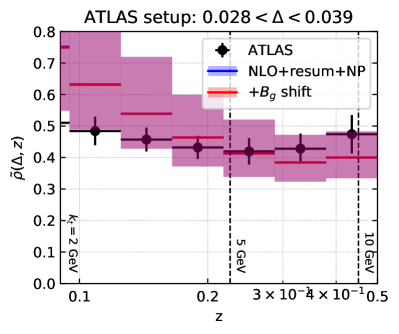
Figure 14: Estimate of the effect of a hard collinear splitting for the largest-$\Delta$ bin of the ATLAS data, using Eqs. (56) and (57).

We do nevertheless wish to investigate the size of the one contribution we have outlined in Eq. (56). It can be included in the all-order resummation via the following redefinition of $t_{\text{soft}}$

$$t_{\text{soft}}=\int_{k_{t}}^{p_{\perp}\Delta}\frac{dq_{t}}{q_{t}}\frac{\alpha_{s}(q_{t})}{\pi}\quad\longrightarrow\quad t_{\text{soft}}^{\text{(shifted)}}=\int_{k_{t}e^{-B_{g}\Delta/R}}^{p_{\perp}\Delta}\frac{dq_{t}}{q_{t}}\frac{\alpha_{s}(q_{t})}{\pi},$$ (57)

which would only affect large values of $\Delta$ where the boundary logarithms are present. The effect of this (ad-hoc) prescription on the largest bin in $\Delta$ is shown in Fig. 14. While the effect is relatively small (in particular, relative to our uncertainties and to the discrepancy with the data), we see that our results move in the right direction. Pending a full treatment of these boundary logarithms — left for future work — the bin closest to the jet edge should be treated with caution. We signal this limitation by shading the corresponding region in red in our overall comparisons with the ATLAS data, Figs. 12 and 13.

Appendix C Validation of the resummation at NLO

(a) slices of fixed angle

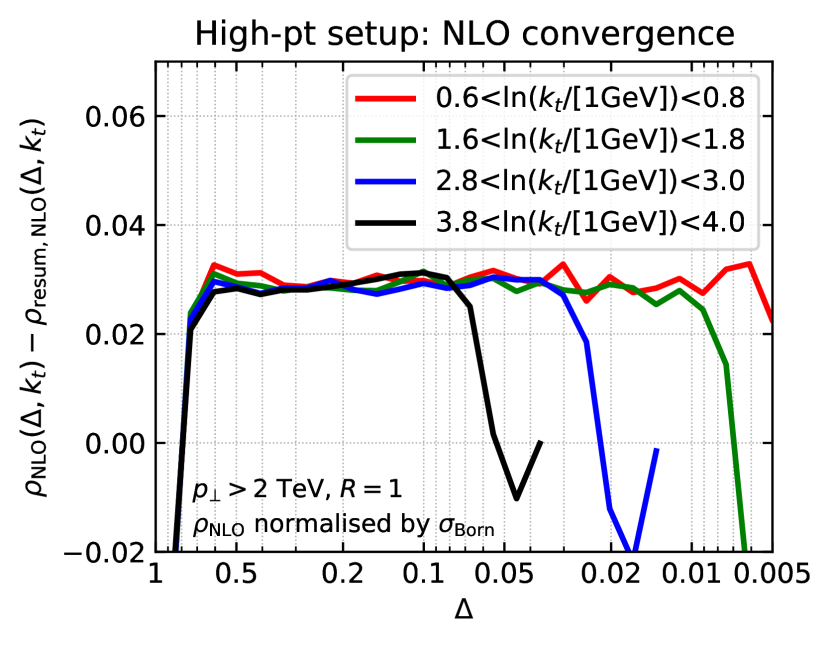
(b) slices of fixed $k_{t}$

Figure 15: Differences between the exact NLO results and the NLO expansion of our resummation for different slices of the Lund plane. Control of single logarithmic terms in our resummation implies that these differences should tend to a constant both for small $k_{t}$ and for small $\Delta$, as observed, except as concerns subleading-$N_{C}$ terms in the small-$k_{t}$, large $\Delta$ region. The exact NLO results are normalised here to the Born-level jet cross-section.

As with any resummed calculation, it is important to check that its expansion to fixed order reproduces the behaviour seen in the exact fixed-order calculation, to within the expected accuracy of the resummation. In our case, this means that, at NLO, one should reproduce all contributions of the form $\alpha_{s}^{2}\ln$, where the argument of the logarithm is any variable in the Lund plane. In practice, one therefore expects the difference $\rho_{\text{NLO}}-\rho_{\text{resum,NLO}}$ to tend to a constant when $k_{t}$ becomes small at a fixed $\Delta$, or when $\Delta\ll 1$ at a fixed $k_{t}$. Fig. 15 shows that this is indeed the case for both limits. We note that, while in the main text of the paper, the NLO Lund-plane density has been normalised to the NLO inclusive jet cross-section, for the purpose of Fig. 15 both $\rho_{\text{NLO}}$ and $\rho_{\text{resum,NLO}}$ have been normalised using the Born-level jet cross-section.

Appendix D Comparison between our calculation and Monte Carlo simulations

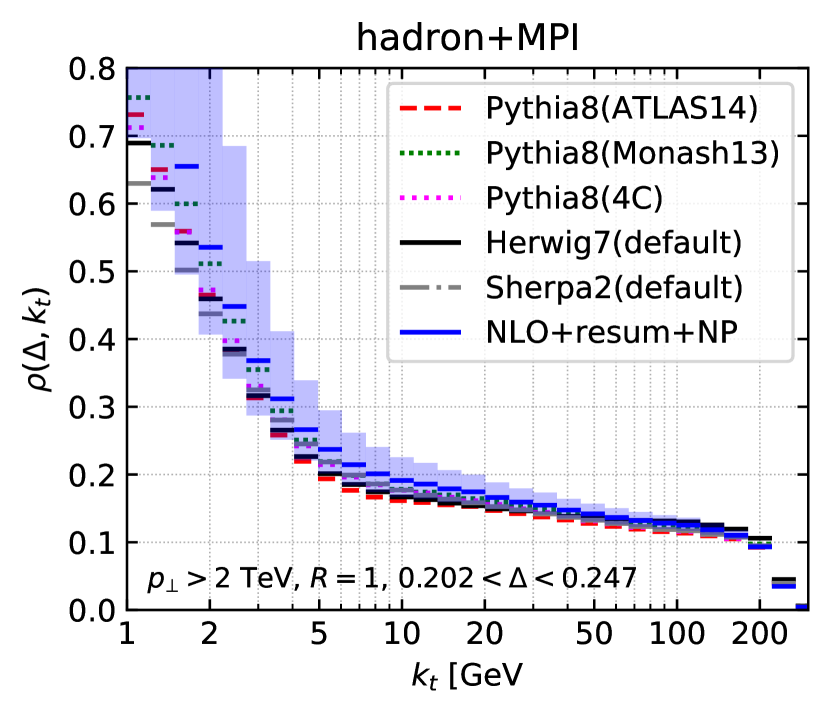
(a) parton level

(b) hadron+MPI level

Figure 16: Comparison between our results for $\rho$ and those obtained with the Monte Carlo generators used to estimate non-perturbative uncertainties.

We show in Fig. 16 a comparison between our analytic calculations and Monte-Carlo simulations for a slice of the Lund plane at constant angle. In Fig. 16(a) we compare our perturbative predictions to parton-level simulations and the (blue) uncertainty band corresponds to our perturbative scale uncertainty. In Fig. 16(b) the comparison is made for the full prediction, including non-perturbative corrections.

At hadron+MPI level, we see a globally-decent agreement between our results and those from each Monte Carlo event generator. At parton-level however, the Herwig7 results are systematically much smaller that our analytic results for $k_{t}$ below $\sim 10$ GeV. This is the main reason for excluding the Herwig7 Monte Carlo when computing the average non-perturbative correction.

Appendix E Non-perturbative corrections for the ATLAS setup

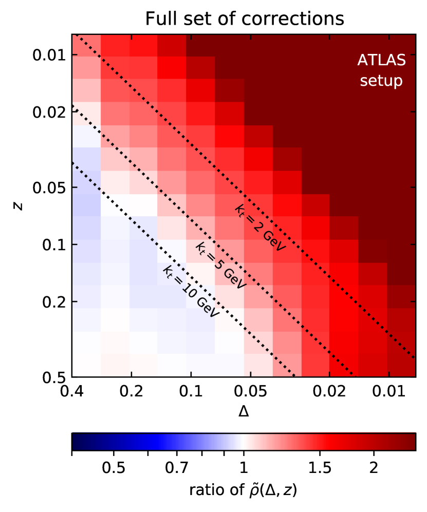
(a) Hadronisation and MPI corrections (all particles)

(b) Effects of the charge track selection.

(c) Final set of non-perturbative corrections.

(d) Uncertainties on hadronisation and MPI corrections.

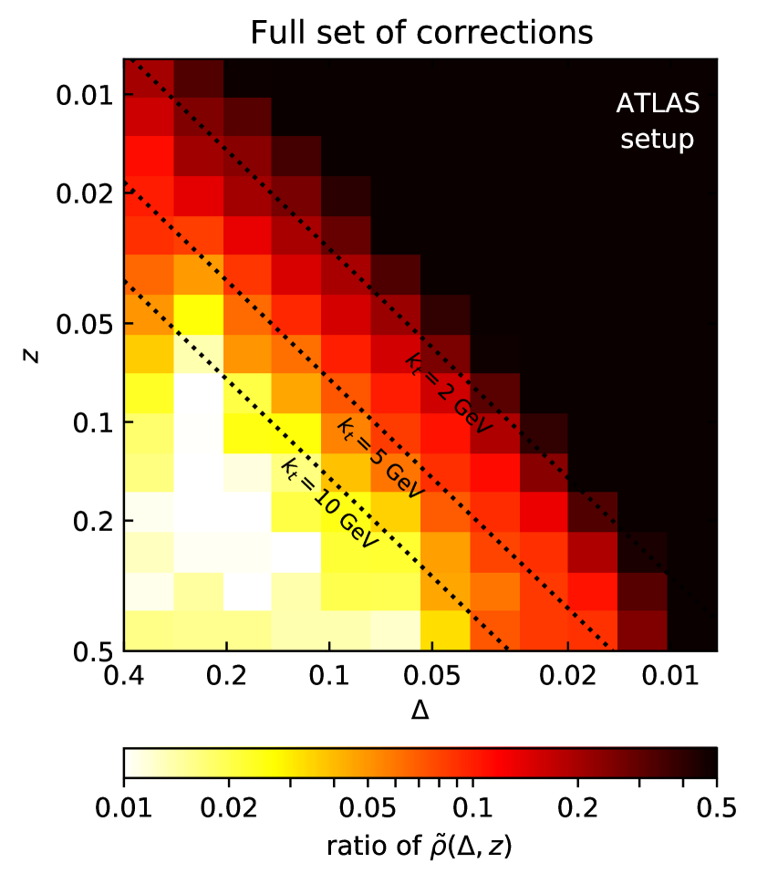
(e) Uncertainties for the charged track selection.

(f) Total uncertainties on non-perturbative corrections.

Figure 17: Non-perturbative effects on $\tilde{\rho}(\Delta,z)$ for the ATLAS setup. The top row shows the average corrections and the lower row shows the associated uncertainties.

The set of non-perturbative corrections included in our calculation of $\tilde{\rho}(\Delta,z)$ for the “ATLAS setup” (cf. section 2) differs from those included in our default “high-$p_{\perp}$ setup.” The main differences are (i) the use of charged tracks instead of all particles, (ii) a slightly different clustering procedure using a radius of $0.4$ for the C/A reclustering, and (iii) the selection of tracks above 500 MeV and within a distance to the jet axis calculated using pseudo-rapidity instead of rapidity.

In Fig. 17, we split the full non-perturbative correction into two separate factors: the corrections due to hadronisation and multi-parton interactions computed on all particles, Fig. 17(a), and the extra corrections associated with the use of charged tracks, the 500 MeV transverse-momentum cut and the track selection based on pseudo-rapidity, Fig. 17(b). The final set of corrections is shown in Fig. 17(c). We clearly see that the use of just charged tracks with momenta greater than $500\,\text{MeV}$ induces a strong reduction of $\tilde{\rho}(\Delta,z)$ beyond the perturbative domain ($k_{t}<2$ GeV) and a positive correction for $k_{t}>2$ GeV. This effect partially cancels the original effect of hadronisation in the region where hadronisation depleted the Lund plane density, i.e. $k_{t}\gtrsim 5$ GeV. The corresponding uncertainties on the non-perturbative corrections are shown in Fig. 17(d)–(f). While the additional corrections associated with the selection of charged tracks add a little to the uncertainty at large $z$, the final pattern of uncertainties is largely unmodified compared to that obtained solely from the hadronisation and MPI uncertainties.

References

- (1) S. Marzani, G. Soyez, and M. Spannowsky, Looking inside jets: an introduction to jet substructure and boosted-object phenomenology, arXiv:1901.10342. [Lect. Notes Phys.958,pp.(2019)].
- (2) A. J. Larkoski, I. Moult, and B. Nachman, Jet Substructure at the Large Hadron Collider: A Review of Recent Advances in Theory and Machine Learning, Phys. Rept. 841 (2020) 1–63, [arXiv:1709.04464].
- (3) R. Kogler et al., Jet Substructure at the Large Hadron Collider: Experimental Review, Rev. Mod. Phys. 91 (2019), no. 4 045003, [arXiv:1803.06991].
- (4) CMS Collaboration, A. M. Sirunyan et al., Search for anomalous electroweak production of vector boson pairs in association with two jets in proton-proton collisions at 13 TeV, Phys. Lett. B 798 (2019) 134985, [arXiv:1905.07445].
- (5) ATLAS Collaboration, G. Aad et al., Measurement of the jet mass in high transverse momentum production at TeV using the ATLAS detector, arXiv:1907.07093.
- (6) ATLAS Collaboration, M. Aaboud et al., Measurement of jet-substructure observables in top quark, boson and light jet production in proton-proton collisions at TeV with the ATLAS detector, JHEP 08 (2019) 033, [arXiv:1903.02942].
- (7) ATLAS Collaboration, M. Aaboud et al., Search for chargino and neutralino production in final states with a Higgs boson and missing transverse momentum at TeV with the ATLAS detector, Phys. Rev. D 100 (2019), no. 1 012006, [arXiv:1812.09432].
- (8) CMS Collaboration, A. M. Sirunyan et al., A multi-dimensional search for new heavy resonances decaying to boosted WW, WZ, or ZZ boson pairs in the dijet final state at 13 TeV, Eur. Phys. J. C 80 (2020), no. 3 237, [arXiv:1906.05977].
- (9) CMS Collaboration, A. M. Sirunyan et al., Combination of CMS searches for heavy resonances decaying to pairs of bosons or leptons, Phys. Lett. B 798 (2019) 134952, [arXiv:1906.00057].
- (10) P. Gras, S. Höche, D. Kar, A. Larkoski, L. Lönnblad, S. Plätzer, A. Siódmok, P. Skands, G. Soyez, and J. Thaler, Systematics of quark/gluon tagging, JHEP 07 (2017) 091, [arXiv:1704.03878].
- (11) C. Frye, A. J. Larkoski, J. Thaler, and K. Zhou, Casimir Meets Poisson: Improved Quark/Gluon Discrimination with Counting Observables, JHEP 09 (2017) 083, [arXiv:1704.06266].
- (12) E. M. Metodiev and J. Thaler, Jet Topics: Disentangling Quarks and Gluons at Colliders, Phys. Rev. Lett. 120 (2018), no. 24 241602, [arXiv:1802.00008].
- (13) A. J. Larkoski and E. M. Metodiev, A Theory of Quark vs. Gluon Discrimination, JHEP 10 (2019) 014, [arXiv:1906.01639].
- (14) H. A. Andrews et al., Novel tools and observables for jet physics in heavy-ion collisions, J. Phys. G 47 (2020), no. 6 065102, [arXiv:1808.03689].
- (15) CMS Collaboration, A. M. Sirunyan et al., Measurement of the Splitting Function in and Pb-Pb Collisions at 5.02 TeV, Phys. Rev. Lett. 120 (2018), no. 14 142302, [arXiv:1708.09429].
- (16) CMS Collaboration, A. M. Sirunyan et al., Measurement of the groomed jet mass in PbPb and pp collisions at TeV, JHEP 10 (2018) 161, [arXiv:1805.05145].
- (17) ALICE Collaboration, S. Acharya et al., Exploration of jet substructure using iterative declustering in pp and Pb–Pb collisions at LHC energies, Phys. Lett. B 802 (2020) 135227, [arXiv:1905.02512].
- (18) Y. Mehtar-Tani and K. Tywoniuk, Groomed jets in heavy-ion collisions: sensitivity to medium-induced bremsstrahlung, JHEP 04 (2017) 125, [arXiv:1610.08930].
- (19) Y.-T. Chien and I. Vitev, Probing the Hardest Branching within Jets in Heavy-Ion Collisions, Phys. Rev. Lett. 119 (2017), no. 11 112301, [arXiv:1608.07283].
- (20) N.-B. Chang, S. Cao, and G.-Y. Qin, Probing medium-induced jet splitting and energy loss in heavy-ion collisions, Phys. Lett. B 781 (2018) 423–432, [arXiv:1707.03767].
- (21) G. Milhano, U. A. Wiedemann, and K. C. Zapp, Sensitivity of jet substructure to jet-induced medium response, Phys. Lett. B 779 (2018) 409–413, [arXiv:1707.04142].
- (22) P. Caucal, E. Iancu, and G. Soyez, Deciphering the distribution in ultrarelativistic heavy ion collisions, JHEP 10 (2019) 273, [arXiv:1907.04866].
- (23) J. Casalderrey-Solana, G. Milhano, D. Pablos, and K. Rajagopal, Modification of Jet Substructure in Heavy Ion Collisions as a Probe of the Resolution Length of Quark-Gluon Plasma, JHEP 01 (2020) 044, [arXiv:1907.11248].
- (24) J. M. Butterworth, A. R. Davison, M. Rubin, and G. P. Salam, Jet substructure as a new Higgs search channel at the LHC, Phys. Rev. Lett. 100 (2008) 242001, [arXiv:0802.2470].
- (25) D. Krohn, J. Thaler, and L.-T. Wang, Jet Trimming, JHEP 02 (2010) 084, [arXiv:0912.1342].
- (26) J. Thaler and K. Van Tilburg, Identifying Boosted Objects with N-subjettiness, JHEP 03 (2011) 015, [arXiv:1011.2268].
- (27) A. J. Larkoski, G. P. Salam, and J. Thaler, Energy Correlation Functions for Jet Substructure, JHEP 06 (2013) 108, [arXiv:1305.0007].
- (28) M. Dasgupta, A. Fregoso, S. Marzani, and G. P. Salam, Towards an understanding of jet substructure, JHEP 09 (2013) 029, [arXiv:1307.0007].
- (29) A. J. Larkoski, S. Marzani, G. Soyez, and J. Thaler, Soft Drop, JHEP 05 (2014) 146, [arXiv:1402.2657].
- (30) A. J. Larkoski, J. Thaler, and W. J. Waalewijn, Gaining (Mutual) Information about Quark/Gluon Discrimination, JHEP 11 (2014) 129, [arXiv:1408.3122].
- (31) G. P. Salam, L. Schunk, and G. Soyez, Dichroic subjettiness ratios to distinguish colour flows in boosted boson tagging, JHEP 03 (2017) 022, [arXiv:1612.03917].
- (32) P. T. Komiske, E. M. Metodiev, and J. Thaler, Energy flow polynomials: A complete linear basis for jet substructure, JHEP 04 (2018) 013, [arXiv:1712.07124].
- (33) F. A. Dreyer, G. P. Salam, and G. Soyez, The Lund Jet Plane, JHEP 12 (2018) 064, [arXiv:1807.04758].
- (34) J. Cogan, M. Kagan, E. Strauss, and A. Schwarztman, Jet-Images: Computer Vision Inspired Techniques for Jet Tagging, JHEP 02 (2015) 118, [arXiv:1407.5675].
- (35) L. de Oliveira, M. Kagan, L. Mackey, B. Nachman, and A. Schwartzman, Jet-images — deep learning edition, JHEP 07 (2016) 069, [arXiv:1511.05190].
- (36) P. T. Komiske, E. M. Metodiev, and M. D. Schwartz, Deep learning in color: towards automated quark/gluon jet discrimination, JHEP 01 (2017) 110, [arXiv:1612.01551].
- (37) G. Louppe, K. Cho, C. Becot, and K. Cranmer, QCD-Aware Recursive Neural Networks for Jet Physics, JHEP 01 (2019) 057, [arXiv:1702.00748].
- (38) S. Egan, W. Fedorko, A. Lister, J. Pearkes, and C. Gay, Long Short-Term Memory (LSTM) networks with jet constituents for boosted top tagging at the LHC, arXiv:1711.09059.
- (39) A. Andreassen, I. Feige, C. Frye, and M. D. Schwartz, JUNIPR: a Framework for Unsupervised Machine Learning in Particle Physics, Eur. Phys. J. C 79 (2019), no. 2 102, [arXiv:1804.09720].
- (40) K. Datta and A. J. Larkoski, Novel Jet Observables from Machine Learning, JHEP 03 (2018) 086, [arXiv:1710.01305].
- (41) P. T. Komiske, E. M. Metodiev, and J. Thaler, Energy Flow Networks: Deep Sets for Particle Jets, JHEP 01 (2019) 121, [arXiv:1810.05165].
- (42) CMS Collaboration, Machine learning-based identification of highly Lorentz-boosted hadronically decaying particles at the CMS experiment, Tech. Rep. CMS-PAS-JME-18-002, July, 2019.
- (43) A. Butter et al., The Machine Learning Landscape of Top Taggers, SciPost Phys. 7 (2019) 014, [arXiv:1902.09914].
- (44) G. Kasieczka, N. Kiefer, T. Plehn, and J. M. Thompson, Quark-Gluon Tagging: Machine Learning vs Detector, SciPost Phys. 6 (2019), no. 6 069, [arXiv:1812.09223].
- (45) H. Qu and L. Gouskos, ParticleNet: Jet Tagging via Particle Clouds, Phys. Rev. D101 (2020), no. 5 056019, [arXiv:1902.08570].
- (46) B. Andersson, G. Gustafson, L. Lonnblad, and U. Pettersson, Coherence Effects in Deep Inelastic Scattering, Z. Phys. C43 (1989) 625.
- (47) M. Dasgupta, F. A. Dreyer, K. Hamilton, P. F. Monni, G. P. Salam, and G. Soyez, Parton showers beyond leading logarithmic accuracy, arXiv:2002.11114.
- (48) ATLAS Collaboration, G. Aad et al., Measurement of the Lund jet plane using charged particles in 13 TeV proton-proton collisions with the ATLAS detector, arXiv:2004.03540.
- (49) L. Cunqueiro and M. Płoskoń, Searching for the dead cone effects with iterative declustering of heavy-flavor jets, Phys. Rev. D 99 (2019), no. 7 074027, [arXiv:1812.00102].
- (50) ALICE Collaboration, N. Zardoshti, First Direct Observation of the Dead-Cone Effect, in 28th International Conference on Ultrarelativistic Nucleus-Nucleus Collisions (Quark Matter 2019) Wuhan, China, November 4-9, 2019, 2020. arXiv:2004.05968.
- (51) Z. Nagy, Next-to-leading order calculation of three jet observables in hadron hadron collision, Phys. Rev. D68 (2003) 094002, [hep-ph/0307268].
- (52) M. Cacciari, G. P. Salam, and G. Soyez, The Anti-k(t) jet clustering algorithm, JHEP 04 (2008) 063, [arXiv:0802.1189].
- (53) Y. L. Dokshitzer, G. D. Leder, S. Moretti, and B. R. Webber, Better jet clustering algorithms, JHEP 08 (1997) 001, [hep-ph/9707323].
- (54) M. Wobisch and T. Wengler, Hadronization corrections to jet cross-sections in deep inelastic scattering, in Monte Carlo generators for HERA physics. Proceedings, Workshop, Hamburg, Germany, 1998-1999, pp. 270–279, 1998. hep-ph/9907280.
- (55) S. Amoroso et al., Les Houches 2019: Physics at TeV Colliders: Standard Model Working Group Report, in 11th Les Houches Workshop on Physics at TeV Colliders: PhysTeV Les Houches, 3, 2020. arXiv:2003.01700.
- (56) V. A. Schegelsky, M. G. Ryskin, A. D. Martin, and V. A. Khoze, A note on rapidity distributions at the LHC, arXiv:1010.2051.
- (57) J. Gallicchio and Y.-T. Chien, Quit Using Pseudorapidity, Transverse Energy, and Massless Constituents, arXiv:1802.05356.
- (58) M. Cacciari and G. P. Salam, Dispelling the myth for the jet-finder, Phys. Lett. B 641 (2006) 57–61, [hep-ph/0512210].
- (59) M. Cacciari, G. P. Salam, and G. Soyez, FastJet User Manual, Eur. Phys. J. C 72 (2012) 1896, [arXiv:1111.6097].
- (60) M. Cacciari, G. P. Salam, and G. Soyez, FastJet contrib, 2014 (accessed, March 7, 2020). https://fastjet.hepforge.org/contrib/.
- (61) S. Catani, B. R. Webber, and G. Marchesini, QCD coherent branching and semi-inclusive processes at large , Nucl. Phys. B349 (1991) 635–654.
- (62) M. Dasgupta, F. Dreyer, G. P. Salam, and G. Soyez, Small-radius jets to all orders in QCD, JHEP 04 (2015) 039, [arXiv:1411.5182].
- (63) R. Ellis, G. Marchesini, and B. Webber, Soft Radiation in Parton Parton Scattering, Nucl. Phys. B 286 (1987) 643. [Erratum: Nucl.Phys.B 294, 1180 (1987)].
- (64) Z.-B. Kang, K. Lee, X. Liu, D. Neill, and F. Ringer, The soft drop groomed jet radius at NLL, JHEP 02 (2020) 054, [arXiv:1908.01783].
- (65) M. Dasgupta and G. P. Salam, Accounting for coherence in interjet E(t) flow: A Case study, JHEP 03 (2002) 017, [hep-ph/0203009].
- (66) M. Dasgupta and G. P. Salam, Resummation of nonglobal QCD observables, Phys. Lett. B512 (2001) 323–330, [hep-ph/0104277].
- (67) A. Banfi, G. Marchesini, and G. Smye, Away from jet energy flow, JHEP 08 (2002) 006, [hep-ph/0206076].
- (68) R. B. Appleby and M. H. Seymour, The Resummation of interjet energy flow for gaps between jets processes at HERA, JHEP 09 (2003) 056, [hep-ph/0308086].
- (69) A. Banfi and M. Dasgupta, Problems in resumming interjet energy flows with clustering, Phys. Lett. B628 (2005) 49–56, [hep-ph/0508159].
- (70) Y. Hatta and T. Ueda, Resummation of non-global logarithms at finite , Nucl. Phys. B874 (2013) 808–820, [arXiv:1304.6930].
- (71) Y. Hagiwara, Y. Hatta, and T. Ueda, Hemisphere jet mass distribution at finite , Phys. Lett. B756 (2016) 254–258, [arXiv:1507.07641].
- (72) A. J. Larkoski, D. Neill, and J. Thaler, Jet Shapes with the Broadening Axis, JHEP 04 (2014) 017, [arXiv:1401.2158].
- (73) M. Cacciari, S. Frixione, M. Mangano, P. Nason, and G. Ridolfi, The t anti-t cross-section at 1.8-TeV and 1.96-TeV: A Study of the systematics due to parton densities and scale dependence, JHEP 04 (2004) 068, [hep-ph/0303085].
- (74) T. Sjöstrand, S. Ask, J. R. Christiansen, R. Corke, N. Desai, P. Ilten, S. Mrenna, S. Prestel, C. O. Rasmussen, and P. Z. Skands, An Introduction to PYTHIA 8.2, Comput. Phys. Commun. 191 (2015) 159–177, [arXiv:1410.3012].
- (75) P. Skands, S. Carrazza, and J. Rojo, Tuning PYTHIA 8.1: the Monash 2013 Tune, Eur. Phys. J. C74 (2014), no. 8 3024, [arXiv:1404.5630].
- (76) R. Corke and T. Sjostrand, Interleaved Parton Showers and Tuning Prospects, JHEP 03 (2011) 032, [arXiv:1011.1759].
- (77) ATLAS Pythia 8 tunes to 7 TeV datas, Tech. Rep. ATL-PHYS-PUB-2014-021, CERN, Geneva, Nov, 2014.
- (78) S. Carrazza, S. Forte, and J. Rojo, Parton Distributions and Event Generators, in Proceedings, 43rd International Symposium on Multiparticle Dynamics (ISMD 13), pp. 89–96, 2013. arXiv:1311.5887.
- (79) G. Corcella, I. G. Knowles, G. Marchesini, S. Moretti, K. Odagiri, P. Richardson, M. H. Seymour, and B. R. Webber, HERWIG 6.5 release note, hep-ph/0210213.
- (80) J. Bellm et al., Herwig 7.0/Herwig++ 3.0 release note, Eur. Phys. J. C76 (2016), no. 4 196, [arXiv:1512.01178].
- (81) J. Bellm et al., Herwig 7.2 Release Note, arXiv:1912.06509.
- (82) T. Gleisberg, S. Hoeche, F. Krauss, M. Schonherr, S. Schumann, F. Siegert, and J. Winter, Event generation with SHERPA 1.1, JHEP 02 (2009) 007, [arXiv:0811.4622].
- (83) ATLAS Collaboration, T. A. collaboration, Measurement of the Lund Jet Plane using charged particles with the ATLAS detector from 13 TeV proton–proton collisions, .
- (84) Les Houches 2017: Physics at TeV Colliders Standard Model Working Group Report, 3, 2018.
- (85) S. Marzani, D. Reichelt, S. Schumann, G. Soyez, and V. Theeuwes, Fitting the Strong Coupling Constant with Soft-Drop Thrust, JHEP 11 (2019) 179, [arXiv:1906.10504].
- (86) Y. L. Dokshitzer and B. Webber, Calculation of power corrections to hadronic event shapes, Phys. Lett. B 352 (1995) 451–455, [hep-ph/9504219].
- (87) J. R. Forshaw, J. Holguin, and S. Plätzer, Building a consistent parton shower, arXiv:2003.06400.
- (88) J. R. Forshaw, J. Holguin, and S. Plätzer, Parton branching at amplitude level, JHEP 08 (2019) 145, [arXiv:1905.08686].
- (89) Z. Nagy and D. E. Soper, Parton showers with more exact color evolution, Phys. Rev. D 99 (2019), no. 5 054009, [arXiv:1902.02105].