Radial oscillations and gravitational wave echoes of strange stars for various equations of state

Abstract

We study the radial oscillations of non-rotating strange stars and their characteristic echo frequencies for three Equations of state (EoSs), viz., MIT Bag model EoS, linear EoS and polytropic EoS. The frequencies of radial oscillations of these compact stars are computed for these EoSs. 22 lowest radial frequencies for each of these three EoSs have been computed. First, for each EoS, we have integrated Tolman-Oppenheimer-Volkoff (TOV) equations numerically to calculate the radial and pressure perturbations of strange stars. Next, the mass-radius relationships for these stars are obtained using these three EoSs. Then the radial frequencies of oscillations for these EoSs are calculated. Further, the characteristic gravitational wave echo frequencies and the repetition of echo frequencies of strange stars are computed for these EoSs. Our numerical results show that the radial frequencies and also echo frequencies vastly depend on the model and on the value of the model parameter. Our results also show that, the radial frequencies of strange stars are maximum for polytropic EoS in comparison to MIT Bag model EoS and linear EoS. Moreover, strange stars with MIT Bag model EoS and linear EoS are found to emit gravitational wave echoes. Whereas, strange stars with polytropic EoS are not emitting gravitational wave echoes.

I Introduction

One of the most interesting areas of study in astrophysics and cosmology is the area of strange matter objects (Farhi1984, ; Witten1984, ; Aclock1988, ). Various authors have been working in this area for a long time, mostly trying to constrain mass and radius profiles of stars formed from strange matter using different Equations of state (EoSs) (overgard1991, ; zdunik2002, ; mart2010, ; Weber2012, ), which are yet to be known exactly. The astrophysical compact objects, which are entirely made of quark matter or strange matter (deconfined $u$, $d$, $s$ quark matter), are known as Strange Stars (SSs) (Aclock1988, ; weber2005, ). These compact stars with extremely high densities are unique probes to study the properties of matter under extreme conditions. The study of such stars (i.e. SSs) has appeared as a subject of considerable interest over the last few decades due to their unusual internal composition, structure and physical properties as compared to other compact objects, like White Dwarf (WD) and Neutron Star (NS) (shapiro2004, ). An indirect approach to study such highly compact stars is asteroseismology (handler2012, ). By observing the radial and non-radial modes of oscillations of a star, one can reveal the stability condition, mass, radius, composition, etc. of the star. Though the radial mode, where a regular change in shape and size of the oscillating body occurs, is the simplest oscillation mode, yet it is a great tool for collecting information about the star. The very first study on such radial mode of oscillations of compact stars were carried out by (Chandrasekhar1964a, ; Chandrasekhar1964b, ). After that, radial modes have been investigated for compact stars, like WD and NS for various nuclear matter EoSs by others (Chanmugam1977, ; Glass1983, ; haensel1989, ). In the paper (Chanmugam1977, ), the radial oscillations of zero-temperature degenerate stars (WD and NS) were calculated for the fundamental and first two excited modes. Using the polytropic model EoS, P. Haensel et al. studied the pulsation properties of NS undergoing a phase transition to quark matter (haensel1989, ). For SSs, using the general relativistic pulsation equation, the eigenfrequencies of radial pulsations were calculated by B. Datta et al. in 1992 (datta1992, ). They also calculated the oscillation time periods. The calculation of radial oscillations of SS and NS for 2 lowest order oscillation modes were reported in vath1992 . In recent studies, G. Panotopoulos and I. Lopes computed radial oscillation modes for SS admixed with dark matter (panotopoulos2017, ; panotopoulos2018, ). Study of the anisotropic SS in non-linear EoS was reported by I. Lopes in (lopes2019, ). The displacements in such radial oscillations can be described mathematically by Sturm- Liouville type differential equations, which yield discrete eigensolutions: the radial mode frequencies of the given model (handler2012, ). A new numerical algorithm to solve Sturm-Liouville differential equations governing the radial oscillations of non-rotating SS (see Sec. III) is reported in (clemente2020, ).

An interesting property of such ultracompact objects is that some of them can reflect or echo the Gravitational Waves (GWs) signal (ferrari2000, ; pani2018, ). In 1978, Yu. G. Ignat’ev and A. V. Zakharov showed that GW can be reflected from sufficiently dense stellar bodies (ignatev1978, ). They calculated the condition of reflection and reflection index for NSs. Recently more authors (abedi2017, ; abedi2019, ; abedi2020, ; conklin2018, ) have reported the possibility of GW Echo (GWE) from the ultracompact objects formed in the merging of massive objects, like Black Holes (BHs) and NSs. The echo signal originating from ultracompact star was first reported in (pani2018, ). For non-spinning, constant-density stars they have calculated the characteristic echo frequency $\approx 72$ Hz at $4.2\sigma$ significance level. Those ultracompact massive post-merger objects formed in GW generation events, which feature a photon sphere can only echo the GWs or can trap the GWs partially. The photon sphere is a surface over a massive star located at $R=3M$, where $R$ is the radius and $M$ is the mass of the star (mannarelli2018, ). In photon sphere, circular photon orbits are possible and are featured by both BHs and ultracompact stars (mannarelli2018, ). Thus the emission of GWE takes place if and only if a star features a photon sphere and also it should be very compact, close to the Buchdhal’s limit radius $R_{B}=9M/4$ (buchdahl, ). Thus for GWE, the compactness of the final compact object should lie in between $1/3$ (to have a photon sphere) and $4/9$ (to emit GWEs at a frequency of tens of Hertz) (pani2018, ; mannarelli2018, ). In the recent GW merging event GW170817, the nature of final supermassive stellar object formed is not clearly established (abbott, ). Considering this final supercompact object as a SS, M. Mannareli and F. Tonneli calculated the corresponding echo frequency using the MIT Bag model EoS (mannarelli2018, ). The authors have explained the reason for considering the final compact remnant as a SS in their paper. For the considered model of SS with $B_{1}=(145\,\mbox{MeV})^{4}$ and $B_{2}=(185\,\mbox{MeV})^{4}$, they have calculated the echo frequency as $\omega_{1,echo}=17$ kHz and $\omega_{2,echo}=27$ kHz.

Based on some possible evidences on the existence of SSs (li, ; henderson, ), and also motivated by previous works mentioned above, in this work we have examined the radial oscillation frequencies and GWE frequencies of SSs for three EoSs, viz., MIT Bag model EoS, linear EoS and polytropic EoS. As the external properties of SSs crucially depend on EoSs, so the oscillation and echo frequencies will be different for different EoSs. Thus the use of three EoSs in this study will enable us to compare the results obtained from three EoSs, which may be useful to constrain these models in the future from the observational data of SSs.

The rest of the paper is organized as follows: In Sec. II we have introduced the EoSs that are considered in this work. In Sec. III, the equations governing the radial oscillations, i.e. the hydrostatic equilibrium Tolman-Oppenheimer-Volkoff (TOV) equations are briefly summarized, and the equations for radial and pressure perturbations are discussed. In Sec. IV, a brief discussion on GWE frequencies is made. The numerical results are given in Sec. V and finally we conclude the paper in Sec. VI. In this work we consider the natural unit system, in which $c=\hbar=1$, i.e. all dimensionful quantities are measured in GeV. Also we assume $G=1$ and adopt the metric convention: $(-,\,+,\,+,\,+)$.

II Equation of States

The physics of very high density matter, like SS matter is still not pretty clear till date. In order to construct a compact star’s model, an EoS has to be specified, which is the relation between the pressure $p$ and the energy density $\rho$. A definite EoS for a compact object can give properties, like mass, the mass-radius relationship, the crust thickness, the cooling rate, etc. In most of the studies on SSs, the most simple MIT Bag model EoS framework is used. As mentioned in the previous section, we have considered three EoSs, viz., the MIT Bag model, linear and polytropic EoSs in order to describe SSs. These three EoSs can be used to describe the structure of SSs in General Relativity (GR). The MIT Bag model EoS is the simplest EoS corresponding to a relativistic gas of deconfined quarks with energy density (haensel, ), and in this model it is considered that a universal pressure, known as the Bag constant, on the surface of any region containing quarks causes the quark confinement (chodosa, ; sharma, ). According to this model, the stiffer EoS of the strange matter has a simple linear form as given by (mannarelli2018, )

$$p=\rho-4\,B,$$ (1)

where $\rho$ is the energy density, $p$ is the isotropic pressure and $B$ is the Bag constant. The original form of this model of hadron structure was presented in 1974 by (chodosa, ; chodosb, ) and used by (Witten1984, ) in his calculation of SS mass-radius relation (alcock, ). For SSs in the MIT Bag model EoSs, the maximum mass $M_{max}$ and radius $R$ vary with the Bag constant $B$ as $\propto B^{-1/2}$ (Witten1984, ). In our study we have considered three values of $B$ as $(190\,\mbox{MeV})^{4}$, $(217\,\mbox{MeV})^{4}$ and $(243\,\mbox{MeV})^{4}$. These values of $B$ are chosen here in order to get physically motivated SS configurations in the sense that they almost lie in the acceptable range of values of $B$ as suggested by (aziz, ; carinhas, ). However, it should be noted that till now no stringent physically acceptable range of $B$ is available. Moreover, this model EoSs give SS configrations with a constant compactness independent of $B$, and within the range of $B$ of our interest the required criterion of maximum mass, radius and compactness for the emission of GWEs are fulfilled.

Besides the simple MIT Bag model EoS, Dey et al. in 1998 (dey, ) developed another model for SSs, in which an interquark vector potential and a density based scalar potential describe the quark interactions (sharma, ). The interquark vector potential is originated from gluon exchange and the density dependent scalar potential is used to restore chiral symmetry at a high density. The EoS obtained from this model can be approximated to a linear form, known as the linear EoS, and is given as

$$p=b\,(\rho-\rho_{s}),$$ (2)

where $b$ and $\rho_{s}$ are two model parameters, specifically $\rho_{s}$ represents the surface energy density and $b$ is a linear constant (rosinska, ). In particular, we have used three values of linear constant, which are $b=0.910$, $0.918$ and $0.926$, and the corresponding values of surface energy density $\rho_{s}$ are taken in this study. For this EoS, the maximum mass and corresponding radius of SS increases slowly with increasing $b$ value. While choosing the said values of $b$ we have kept in mind the conditions for emitting GWE frequency from SS, which impose the restriction that compactness of SS should lie within $0.33$ and $0.44$. Under this restriction and the condition for causality $0.710$ is the minimum and $1.000$ is the maximum values of $b$, and so our chosen values of $b$ are well within the allowed compactness range of SSs emitting GWEs.

It is also possible to describe compact stars using polytropic EoS. Hence, in this work we have used also the following polytropic EoS to investigate the behaviour of SSs in GR (tooper1, ; tooper2, ; thiru, ; Herrera, ; kokkotas, ):

$$p=k\,\rho^{\,\Gamma},$$ (3)

where $k$ is the polytropic constant, $\Gamma$ is the polytropic exponent with $\Gamma=1+1/n$, $n$ being the polytropic index. This EoS is one of the primitive polytropic relation describing compact stars. It should be noted that a variation in polytropic index is closely related to different stellar structures. Here we have chosen three different values of polytropic exponent, viz., $1.5$, $1.67$ and $2$ as guess values to describe the structure of SSs. The polytropic constant $k$ depends on central pressure and density of compact stars (tooper2, ). Thus the choice of central density and central pressure highly influences the value of k. For $\Gamma=1.5$, the exact solutions for relativistic polytropes with a polytropic EoS have been found by Thirukkanesh and Ragel (thiru, ). Their study shows that a polytropic compact object with $n=2$ ($\Gamma=1.5$) is viable to experimental results. For $\Gamma=1.5$ we have chosen $k=7.6\times 10^{38}$ corresponding to a suitable central density and central pressure of SSs. This value of $k$ is obtained by setting $c=\hbar=G=1$ and using the relation: $1$ GeV = $1M_{P}/(1.22\times 10^{19})$, where $M_{P}$ is the Planck mass, which is taken as unity in this work. Values of $k$ for other two $\Gamma$s are calculated accordingly. Thus, for $\Gamma=1.67$ corresponding to $n=1.5$, $k=0.05\,{\mbox{fm}^{8/3}}\approx 1.7\times 10^{51}$ is taken (ray, ). We have chosen some higher value of $\Gamma$, i.e. $\Gamma=2$ corresponding to $n=1$ and $k=1.1\times 10^{-4}\,{\mbox{fm}^{3}}\,{\mbox{MeV}^{-1}}\approx 4.6\times 10^{77}$ (lattimer, ). As it is well known that compact stars, like neutron stars are best described for the polytropic exponent $\Gamma$s lying in the range of $2$ and $3$ (lattimer, ; kokkotas, ; ns, ). So, in order to describe SSs we have chosen the lower value of polytropic exponent, i.e. $\Gamma=2$ from this range. The value $\Gamma=1.67$ is taken as intermediate value between $1.5$ and $2$ for the corresponding values of $n$.

Once the EoS of a star is known, the TOV equations can be integrated numerically to calculate the macroscopic features of the star, such as its mass and radius.

III Radial oscillations of strange stars

To study a relativistic star in GR one needs to solve first the Einstein’s field equations for a given spacetime metric. The Einstein’s field equations in a compact form is given by

$$G_{\mu\nu}=R_{\mu\nu}-\dfrac{1}{2}g_{\mu\nu}R=8\pi T_{\mu\nu},$$ (4)

where $G_{\mu\nu}$ is the Einstein tensor, $g_{\mu\nu}$ is the metric tensor, $T_{\mu\nu}$ is the energy-momentum tensor, $R_{\mu\nu}$ is the Ricci tensor and $R$ is the Ricci scalar. For a spherically symmetric static system or stellar object, we have to use the Schwarzschild metric, given as

$$ds^{2}=-\,e^{\chi(r)}dt^{2}+e^{\lambda(r)}dr^{2}+r^{2}\,d\Omega^{2},$$ (5)

where as usual $t$ and $r$ respectively represent the time and space coordinates and $d\Omega^{2}=d\theta^{2}+\sin^{2}\theta\,d\phi^{2}$; $\theta$ and $\phi$ are polar and azimuthal angles. The metric parameters $\chi$ and $\lambda$ are functions of $r$ only and can be replaced by

$$e^{-\,\chi}=e^{\lambda}=\dfrac{1}{1-2M/r},$$ (6)

where $M$ is the mass at the radius $R$ of the star and $r<R$. In GR, when a star is in hydrostatic equilibrium then its interior structure is described by the TOV equations (tolman, ; tov, ), which are derived by solving the Einstein’s Eqs. (4) for the Schwarzschild metric (5). So, for simplicity if we neglect the rotation of the compact stellar objects, then the structure of such objects can be obtained by solving the TOV equations, which are

$$\dfrac{d\chi}{dr}= \;-\dfrac{2}{\rho+p}\dfrac{dp}{dr},$$ (7)

$$\dfrac{dm}{dr}= \;4\pi\rho\,r^{2},$$ (8)

$$\dfrac{dp}{dr}= \;-(\rho+p)\left(\frac{m}{r^{2}}+4\pi p\,r\right)\left(1-\frac{2m}{r}\right)^{-1},$$ (9)

where $\rho=\epsilon/c^{2}$ is the energy density, c being the speed of light in vacuum which is considered to be equal to unity in this work.

The set of hydrostatic equilibrium equations is an initial value problem and can be solved numerically. Now for some given EoSs, the TOV Eqs. (8) and (9) are to be integrated with initial conditions : (i) mass at the centre is zero, i.e. $m(r=0)=0$ and (ii) pressure at the centre becomes the central pressure, i.e. $p(r=0)=p_{c}$. Moreover, the radius of the star can be determined by the fact that the energy density vanishes at the surface, i.e. $\rho(r=R)=0$. At the surface of the star the mass can be given as $m(r=R)=M$. And finally the metric term $\chi$ can be calculated from Eq. (7) using the boundary condition:

$$\chi(R)=\ln\,(1-\dfrac{2M}{R}).$$ (10)

The solution of TOV equations for a particular star will give the information about the star and using these information the asteroseismic behaviour of that star can be revealed.

In 1964, S. Chandrasekhar for the first time established equations that govern the radial oscillations of a gas sphere in the general relativistic framework taking into account radial and pressure perturbations (Chandrasekhar1964a, ; Chandrasekhar1964b, ). Defining the dimensionless variables $\xi=\Delta r/r$ and $\eta=\Delta p/p$, where $\Delta r$ is the radial perturbation and $\Delta p$ is the corresponding Lagrangian perturbations of the pressure, the Chandrasekhar’s equations of radial and pressure perturbations can be written as (Chandrasekhar1964a, ; Chandrasekhar1964b, ; Chanmugam1977, ; vath1992, ; panotopoulos2017, )

$$\small{\dfrac{d\xi}{dr}=-\,\dfrac{1}{r}\left(3\xi+\dfrac{\eta}{\gamma}\right)-\dfrac{dp}{dr}\dfrac{\xi}{p+\rho}},$$ (11)

$$\dfrac{d\eta}{dr}=\xi\left[\omega^{2}r\left(1+\dfrac{\rho}{p}\right)e^{\lambda-\chi}-\dfrac{dp}{dr}\dfrac{4}{p}-8\pi(p+\rho)\,r\,e^{\lambda}\right.\\ \left.+\;\dfrac{r}{p\,(p+\rho)}{\left(\dfrac{dp}{dr}\right)}^{2}\right]+\eta\left[-\,\dfrac{\rho}{p\,(p+\rho)}\dfrac{dp}{dr}-4\pi(p+\rho)\,r\,e^{\lambda}\right],$$ (12)

where $\omega$ is the eigenfrequency of vibration and $\gamma$ is the relativistic adiabatic index, which plays a significant role in the dynamical stability of a star Chanmugam1977 and is given by

$$\gamma=\dfrac{dp}{d\rho}(1+\rho/p).$$ (13)

This system of coupled first order differential Eqs. (11) and (12) contains singularities at the centre and the surface. To solve such system of equations we need two boundary conditions, one at the centre as $r\rightarrow 0$ and other at the surface of the star, i.e. at $r=R$. As $r\rightarrow 0$, the coefficient of $1/r$ in Eq. (11) must vanish. So the condition that must satisfy at the centre or the first boundary condition is

$$3\,\gamma\,\xi+\eta=0.$$ (14)

The second boundary condition demands that as $r\rightarrow R$, $\rho\rightarrow 0$, $p\rightarrow 0$ and $dp/dr\rightarrow 0$. Again as $p\rightarrow 0$, $p/\rho\rightarrow 0$ and $\rho/p\rightarrow\infty$. Therefore the coefficient of $\rho/p$ in Eq. (12) must vanish as $r\rightarrow R$. Thus using Eq. (9) in Eq. (12) from this condition it can be found that

$$\eta=\xi\left[-\,4+\left(1-\dfrac{2M}{R}\right)^{-1}\left(-\,\dfrac{M}{R}-\dfrac{\omega^{2}R^{3}}{M}\right)\right]$$ (15)

must be satisfied at the surface of the star. Here $M$ and $R$ are the mass and radius of the star respectively. These coupled differential Eqs. (11) and (12) along with the boundary conditions Eqs. (14) and (15) form a two point boundary value problem of the Sturm-Liouville type and has real eigenvalues $\omega_{0}^{2}<\omega_{1}^{2}<\ldots<\omega_{n}^{2}<\ldots$, where $\omega_{n}$ are the eigenfrequencies of oscillations, which have $n$ nodes (cox80, ). The $n=0$ mode is called as the fundamental or $f$-mode. Since $\omega$ is real for $\omega^{2}>0$, hence the solution is purely oscillatory in a stable state. But for $\omega^{2}<0$, the frequency $\omega$ becomes imaginary and it corresponds to an exponentially growing unstable radial oscillations. We solved this couple differential equations by using shooting method as described by G. Panotopoulus in (panotopoulos2017, ). First we have calculated the dimensionless quantity $\bar{\omega}=\omega\,t_{0}$, where $t_{0}=1$ ms and then the frequencies are calculated by using the relation :

$$\nu=\dfrac{\overline{\omega}}{2\pi}\;\;\mbox{kHz}.$$ (16)

The frequency $\nu$ is allowed to take some particular values called the eigenvalues $\nu_{n}$. Each values of $\nu_{n}$ corresponds to a specific radial oscillation mode of the star. So it can be inferred that a radial oscillation mode of a star is associated with the eigenvalue $\nu_{n}$ and the corresponding eigenfunctions $\xi_{n}$ and $\eta_{n}$.

IV Gravitational wave echo frequencies from strange stars

The collapse of two massive objects lead to the formation of ultra-compact objects. The resulting compact object may be an SS. If such stars fulfill some criterion, they can echo GWs. Considering the final object as an SS and featuring a photon sphere, the typical echo frequency emitted can be calculated. As mentioned earlier, the surface of photon sphere is located at $R=3M$ and the Buchdhal’s limit radius is $R=9M/4$. Thus to emit GWE, the compact stellar object should have compactness $M/R$ larger than $1/3$ and smaller than $4/9$.

To calculate the frequency of GWE, the TOV Eqs. (7) – (9) together with a EoS are to be solved. For this purpose we consider the EoSs described in Sec. II. Among these EoSs, those equations are found to be useful which can mimic a star with larger compactness. When the masses of SSs are sufficiently large, the gravitational pull becomes larger and will give a more compact configuration. As we have mentioned earlier that only those compact stellar objects having compactness within the photon sphere line and Buchdahl’s limit can emit GWEs, i.e. the mass-radius curves should cross the photon sphere line, but do not approach the Buchdahl’s limit line. To check this criterion, EoSs given in Eqs. (1) – (3) are used in this study. In Fig. 1 the mass-radius curves for these EoSs are shown. Also the photon sphere limiting line, the Buchdahl’s limit line and black hole line are shown in the figure. It is seen that the EoSs given by Eq. (1) and Eq. (2) with considered values of constants can only give the required compactness and cross the photon sphere limit line. Whereas in the case of polytropic EoS, the last stable configuration with largest mass is small and hence the compactness.

The typical GWE time can be given as the light crossing time from the centre of the astrophysical object to the photon sphere (pani2018, ; mannarelli2018, ),

$$\tau_{echo}=\int_{0}^{3M}\!\!\!\!\dfrac{1}{\sqrt{e^{\,\chi(r)}(1-2m(r)/r)}}\;\mathrm{d}r.$$ (17)

The terms $m(r)$ and $\chi(r)$ can be evaluated by solving Eqs. (7) – (9) for EoS models considered. Using this relation for the characteristic echo time, the GWE frequency can be calculated from the relation $\omega_{echo}=\pi/\tau_{echo}$ (cardoso1, ) and the corresponding repetition frequency of the echo signal can be calculated using the relation $\omega_{repetion}=1/(2\,\tau_{echo})$. In general echoes have two natural frequencies: the harmonic or resonance frequencies and the quasi-normal mode frequencies (abedi2019, ). We refer the harmonic or resonance frequency as the repetition frequency, as it actually corresponds to the repetition frequency of the echo signal. The results obtained for these EoSs are discussed in Sec. V.

V Numerical results and discussion

As described above, in this study we have computed radial frequencies of $22$ lowest order radial oscillation modes and GWE frequencies of different SSs. For the typical SS models considered here, we have chosen maximum masses of SSs, $M\leq 3.3\,M_{\odot}$ and radii $R\leq 14$ km. The behaviour of such stars is different from other compact stars and this can be visualized by observing their mass-radius relationships. As already mentioned in the last section, in Fig. 1 we have plotted the mass-radius relationships for the EoSs described in Sec. II. The mass-radius relation for SSs in polytropic EoS is following a pattern somewhat different from the other two EoSs. It is because, such EoS will give stars with smaller value of compactness. For other values of model parameter which are not included in Fig. 1, the respective compactness and mass-radius behaviour can be found in Table 1. In this table we have shown the values of mass, radius and compactness of SSs obtained for different EoSs. It would be appropriate to mention here that according to stability analysis of hydrostatic equilibrium configuration of stellar structure under polytropic EoS, the equilibrium mass $M$ of such structure varies with respect to its central density $\rho_{c}$ as

$$\frac{dM}{d\rho_{c}}\propto\Gamma-\frac{4}{3}.$$

This relation implies that the equilibrium stellar configuration with $dM/d\rho_{c}\geq 0$ are stable, but those with $dM/d\rho_{c}<0$ are unstable (shapiro2004, ). In view of this stability condition, all three values of $\Gamma=1.5,1.67$ and $2$, we have considered in this study, should give the stable mass-radius relationship. So, the mass-radius curve for the polytropic EoS with $\Gamma=2$ in Fig. 1 can be viewed as the hydrostatic equilibrium stellar configurations with different central densities who satisfy the same polytropic EoS. Thus the highest point (along y-axis) on the curve corresponds to maximum mass and density of a stable star, whereas the lowest point with maximum radius gives the lowest mass and density of a stable star that are governed by polytropic EoS with $\Gamma=2$ in hydrostatic equilibrium. In the following subsections we discuss our numerical results on radial oscillation frequencies and GWEs.

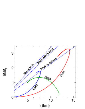
Figure 1: Mass-radius relationships of various SSs for the MIT Bag model EoS, linear EoS and polytropic EoS showing photon sphere limit, Buchdahl’s limit and black hole limit lines. Here EoS1 represents the MIT bag model EoS with $B=(190\,\mbox{MeV})^{4}$, EoS2 is for the linear EoS with $b=0.910$, and the polytropic EoS with $\Gamma=2$ is denoted as EoS3. Although this figure is plotted for one model parameter of each EoS, the patterns of this figure are applicable to all chosen parameters of the corresponding EoSs.

Table 1: Mass, radius and compactness of SSs for three EoSs with different model parameters.

EoSs	Model	Radius R	Mass M	Compactness
	Parameter	(in km)	(in $M_{0}$)	(M/R)
MIT Bag model	$B=(190\,\mbox{MeV})^{4}$	13.766	3.295	0.3540
	$B=(217\,\mbox{MeV})^{4}$	10.630	2.544	0.3540
	$B=(243\,\mbox{MeV})^{4}$	8.456	2.024	0.3540
Linear EoS	$b=0.910$	7.535	1.775	0.3484
	$b=0.918$	7.816	1.844	0.3489
	$b=0.926$	8.128	1.920	0.3494
Polytropic EoS	$\Gamma=1.50$	11.200	0.814	0.1081
	$\Gamma=1.67$	7.980	0.964	0.1790
	$\Gamma=2.00$	7.500	1.350	0.2600

V.1 Radial oscillation frequencies of SSs

As mentioned in Sec. III, the radial and pressure perturbation Eqs. (11) and (12) are the coupled differential equations of Sturm-Liouville type whose eigenvalue solutions give the various modes of oscillations, e.g. for $n=0$, we get the fundamental mode, for $n=1$ the first overtone or the pressure $p_{1}$ mode, for $n=2$ the second overtone or the $p_{2}$ mode and so on. The displacement and pressure perturbation variables $\xi(r)$ and $\eta(r)$ obtained respectively from the solutions of these equations are plotted for various modes, mainly for lower order ($n=0,1,2$) modes and for higher order ($n=20,22$) modes, against the distance $r$ (in km) from the centre of SS. Figs. 2, 3 and 4 correspond to the plots of the pressure perturbations with respect to distance from the centre of the star for various modes oscillations for MIT Bag model EoS, linear EoS and polytropic EoS respectively. For these models, the pressure perturbations $\eta_{n}(r)$ are larger near the centre and near the surface of the star. However $\eta_{n}(r)$ is slightly smaller near the surface of the stars with these EoSs. The values of pressure perturbations are found to vary from model to model. Also, for a certain model with different model parameters significant variations are noticed in pressure perturbations.

     

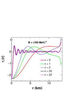
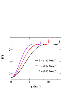
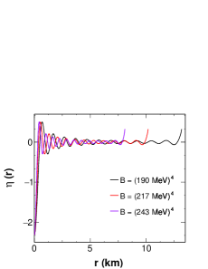
Figure 2: Behaviours of pressure perturbation parameter $\eta(r)$ as a function of distance from the centre of SS for different modes of oscillations obtained from the numerical solution of Eq. (12) using the MIT Bag Model EoS. Left plot is with Bag constant $B={(190\,\mbox{MeV})}^{4}$ for both low order modes $n=0,1,2$ and highly excited modes $n=20,22$. The other two plots are with three Bag constants, viz., $B={(190\,\mbox{MeV})}^{4}$, ${(217\,\mbox{MeV})}^{4}$ and ${(243\,\mbox{MeV})}^{4}$ for $f$-mode (middle panel) and $p_{22}$-mode (right panel) of oscillations respectively.

For the MIT Bag model with $B={(190\,\mbox{MeV})}^{4}$, the variations of $\eta_{n}(r)$ with respect to $r$ for all said modes are shown in the left plot of Fig. 2. The dependence of $\eta_{n}(r)$ on Bag constant $B$ is shown in other two plots of this figure. It is seen that for both lower (middle plot of Fig. 2) and higher (right plot of Fig. 2) order modes, the pressure perturbations varies noticeably with $B$. As different values of Bag constant of MIT Bag model will represent different stars, so the pressure perturbation along the radius of the star will be different for different Bag constants. The Bag model corresponding to $B={(190\,\mbox{MeV})}^{4}$ gives a star with the maximum radius than other two values of $B$. The values of pressure perturbations $\eta_{n}(r)$ for MIT Bag model with $B={(190\,\mbox{MeV})}^{4}$, ${(217\,\mbox{MeV})}^{4}$ and ${(243\,\mbox{MeV})}^{4}$ are almost same near the centre of the star. But at the surface of the star values of $\eta_{n}(r)$ are found to be different slightly as the radius of the star is different with these three different values of $B$.

As mentioned above, in Fig. 3 pressure perturbations for linear EoS are plotted against the radial distance of the star. In the left plot of this figure the perturbations obtained by using the linear constant $b=0.910$ are shown for five modes, three of them are lowest order modes and two are highest order modes as in the earlier case. The perturbations are larger near the centre and surface of the star. In the middle and right plots of Fig. 3 lower and higher order modes are drawn respectively for three values of linear constants, viz., $b=0.910$, $0.918$ and $0.926$. It is seen that for the linear EoS with these three constants all modes of perturbations in pressure are almost same from centre to near the surface of the star. The highest value of $b$, i.e. $0.926$ considered here corresponds to the star with maximum radius and the lowest value $b=0.910$ gives star of minimum radius.

     

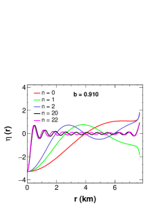
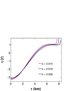
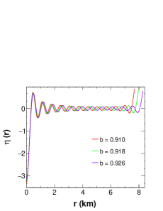
Figure 3: Behaviours of pressure perturbation parameter $\eta(r)$ as a function of distance from the centre of SS for different modes of oscillations obtained from the numerical solution of Eq. (12) using the linear EoS. The first plot is with linear constant $b=0.910$ for both low order modes $n=0,1,2$ and highly excited modes $n=20,22$, and the last two plots are for $f$-mode and $p_{22}$-mode of oscillations respectively with linear constants $b=0.910$, $0.918$ and $0.926$.

For polytropic EoS, the variation of pressure perturbations $\eta_{n}(r)$ along the radial distance $r$ of the star is shown in Fig. 4 as mentioned earlier. Similar to the cases of linear EoS and MIT Bag model EoS, the perturbations at the surface of the star are nearly equal (but not exactly) to the values near the centre of the star. In the left plot of the figure the perturbed pressures are shown for three lower order modes and two higher order modes as in the cases of other EoSs. The middle and the right plots are to show the variation of $\eta(r)$ with $\Gamma$. For all these modes the perturbations are found to follow almost the same rule: larger near the centre and near the surface of the star. However, there is a small exception for the case of $n=0$ mode. In this case the amplitude of pressure perturbation shows the decreasing trend towards the surface of the star, especially for smaller values of $\Gamma$. For the three values of $\Gamma$ considered here, the variation in $\eta_{n}(r)$ with radius is following the same pattern with the expecption as mentioned above and the largest $\Gamma$ gives the star with smallest radius.

     

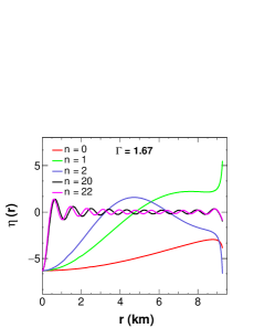
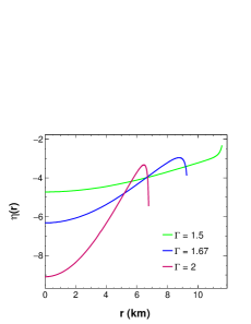
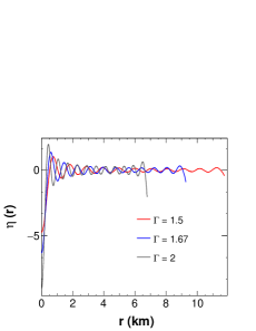
Figure 4: Behaviours of pressure perturbation parameter $\eta(r)$ as function of radial distance of SS for low order oscillation modes $n=0,1,2$ and highly excited modes $n=20,22$ obtained from the numerical solution of Eq. (12) using polytropic EoS for $\Gamma=1.67$ [left plot]. Same for $f$-mode [middle plot] and $p_{22}$-mode [right plot] with different values of polytropic exponent $\Gamma$.

The radial perturbations of SSs with respect to radial distance obtained from the numerical solution of Eq. (11) using different EoSs are shown in Fig. 5, 6 and 7. Unlike the variation of pressure perturbations, which are larger near the centre of the star and also near the surface of the star, radial perturbations are maximum near the centre of the star only. That is the radial perturbations gradually decrease with along the radial distance and become minimum near the surface of the star. For MIT Bag model with $B={(190\,\mbox{MeV})}^{4}$, the variation of $\xi_{n}(r)$ with $r$ is shown in the left plot of Fig. 5. The other two plots of this figure are to show how these radial perturbations depend on the Bag constants. In the middle plot the dependence of low order oscillation modes on $B$ is shown and in the right plot it is shown for higher order modes. The low value of $B$ corresponds the maximum radius as clear from the middle and right plots of the figure.

     

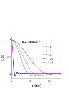
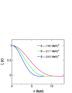
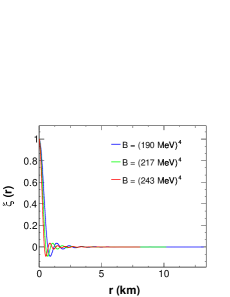
Figure 5: Behaviours of radial perturbation parameter $\xi(r)$ as a function of distance from the centre of SS for different modes of oscillations obtained from the numerical solution of Eq. (11) using the MIT Bag Model EoS. First plot is with Bag constant $B={(190\,\mbox{MeV})}^{4}$ for both low order modes $n=0,1,2$ and highly excited modes $n=20,22$, and the other two plots are for $f$-mode and $p_{22}$-mode of oscillations respectively with three values of $B={(190\,\mbox{MeV})}^{4}$, ${(217\,\mbox{MeV})}^{4}$ and ${(243\,\mbox{MeV})}^{4}$.

Same study is made for the linear EoS with three different linear constants as earlier, which is represented in Fig. 6. It is already seen that stars given by different linear constants have slightly varying radii. The variation of $\xi_{n}(r)$ for different $b$ is found to be smaller than the variation of $\xi_{n}(r)$ for stars (i.e. for different $B$) represented by MIT Bag models. In the left plot different modes of $\xi(r)$ is plotted against radial distance of the star for $b=0.910$. The middle and the right plots of this figure correspond to the variation of $\xi_{n}(r)$ with different values of $b$ for low order modes and higher order modes respectively. As in the case of pressure perturbations, the radial perturbations also show that for the star with $b=0.926$ will have larger radius (but slightly) and hence has maximum perturbation compared to the other two values of $b$.

     

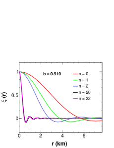
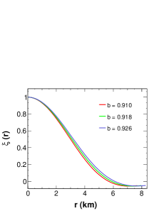
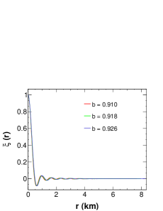
Figure 6: Behaviours of radial perturbation parameter $\xi(r)$ as a function of distance from the centre of SS for different modes of oscillations obtained from the numerical solution of Eq. (11) using the linear EoS. The first plot is with $b=0.910$ for both low order modes $n=0,1,2$ and highly excited modes $n=20,22$, and the last two plots are with $b=0.910$, $0.918$ and $0.926$ for $f$-mode and $p_{22}$-mode of oscillations respectively.

For polytropic EoS, with polytropic index $\Gamma=1.5$, $1.67$ and $2$ the radial perturbations $\xi_{n}(r)$ are plotted for different oscillation modes of the star in Fig. 7. As in the case of other EoSs, for this model, $\xi(r)$ is maximum near the centre of the star and minimum near the surface. The middle and right plot of this figure show the variation of $\xi_{n}(r)$ with different $\Gamma$ values. We have seen that $\xi_{n}(r)$ vary significantly with $\Gamma$, specially in low order modes.

     

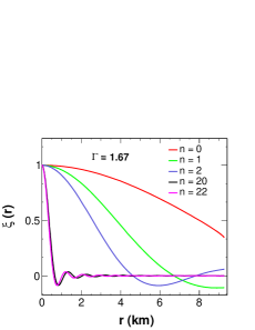
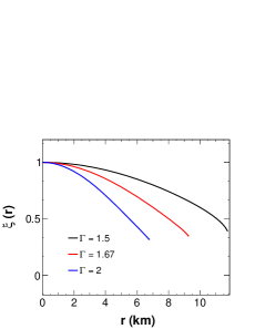
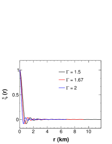
Figure 7: Behaviours of radial perturbation parameter $\eta(r)$ as a function of radial distance of SS for low order oscillation modes $n=0,1,2$ and highly excited modes $n=20,22$ obtained from the numerical solution of Eq. (11) using polytropic EoS for $\Gamma=1.67$ [left plot]. Same for $f$-mode [middle plot] and $p_{22}$-mode [right plot] with various polytropic exponent $\Gamma$ values.

As a comparative analysis of the predictions of all three models considered in this work, we have shown the variation of pressure and radial perturbations for these three model EoSs in Fig. 8 and Fig.9 respectively. In the left plot of Fig. 8 the comparison of variation of $f$-mode of pressure perturbations with the star radial distance is represented. The right plot of this figure is shown the same for the $p_{22}$ oscillation mode of the star. As clear from this figure, the linear EoS is predicting a star of smallest radius. For all these three EoSs, the pattern of variation of $\eta_{n}(r)$ is same, maximum near the centre and near the surface of the star.

     

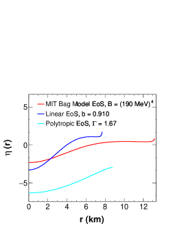
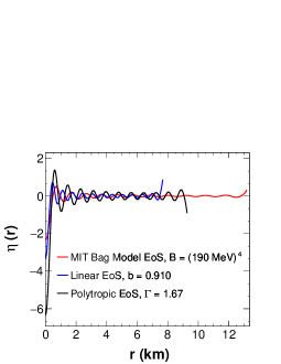
Figure 8: Variation of pressure perturbation parameter $\eta(r)$ with radial distance of SS for three EoSs. The left plot is for the $f$-mode and the other plot is for the $p_{22}$-mode.

In Fig. 9, the radial perturbations are compared for these three different pressure-energy density relations. In the left plot the results of $f$-mode and in the right plot the results of $p_{22}$-mode are compared. Unlike the pressure perturbations, the radial perturbation values are found to maximum near the centre of each stars and are found to follow the same pattern in all EoSs. In this case also the linear EoS gives the star with the smallest radius.

     

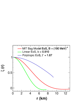
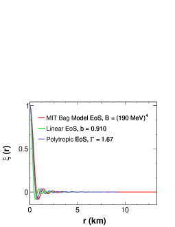
Figure 9: Variation of radial perturbation parameter $\xi(r)$ with radial distance of SS for three EoSs. The left plot is for the $f$-mode and the right plot is for the $p_{22}$-mode.

Table 2 shows all calculated radial oscillation frequencies of such stars for the aforementioned EoSs obtained by using all three chosen constant parameters in each EoS. Here the oscillation frequencies of respective 22 modes from the $f$-mode (in order $n$) are given in kHz. It is seen that for the MIT bag model EoS and the polytropic EoS, the oscillation frequencies of all modes increase with the increasing values of constant parameters, while the situation is opposite in the case of linear EoS. Thus, individually frequencies are maximum for $B=(243\,\mbox{MeV})^{4}$ of MIT Bag model EoS, for $b=0.910$ of linear EoS and for $\Gamma=2$ of polytropic EoS. But, among these EoSs polytropic EoS with $\Gamma=2$ gives highest maximum frequencies of radial oscillations. Moreover, for the purpose of visualization we have shown in Fig. 10 the graphical representation of comparison of maximum radial oscillation frequencies obtained for each EoSs with the said respective constant parameters.

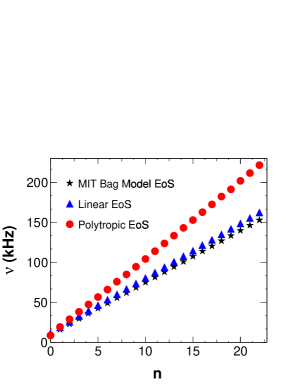
Figure 10: Comparative variation of radial oscillation frequencies $\nu_{n}$ with respect to oscillation modes (n) for the MIT Bag model EoS (black point) with $B=(243\,\mbox{MeV})^{4}$, linear EoS (blue points) with $b=0.910$ and polytropic EoS (red points) with $\Gamma=2$. These are maximum frequencies for each mode given by these EoSs for these respective constant parameters.

Table 2: Radial oscillation frequencies $\nu_{n}$ in kHz for three EoSs. Rows under each EoS are for smaller to bigger values of respective constant parameter. These are $B=(190\,\mbox{MeV})^{4}$, $(217\,\mbox{MeV})^{4}$ and $(243\,\mbox{MeV})^{4}$ for the MIT Bag model EoS; $b=0.910$, $0.918$ and $0.926$ for the linear EoS; and $\Gamma=1.5$, $1.67$ and $2$ for the polytropic EoS.

Modes (Order n)		MIT Bag model EoS			Linear EoS			Polytropic EoS
$f$ (0)	5.08	6.58	8.27	11.44	10.86	10.28	1.57	4.71	8.73
$p_{1}$ (1)	9.88	12.79	16.08	18.85	17.98	17.12	9.26	12.48	19.28
$p_{2}$ (2)	14.08	18.24	22.93	25.88	24.72	23.57	14.56	18.84	28.85
$p_{3}$ (3)	18.15	23.50	29.54	32.78	31.34	29.89	19.57	24.90	38.15
$p_{4}$ (4)	22.16	28.70	36.08	39.63	37.90	36.16	24.46	30.99	47.37
$p_{5}$ (5)	26.15	33.87	42.58	46.45	44.43	42.41	29.27	37.25	56.63
$p_{6}$ (6)	30.14	39.04	49.07	53.26	50.96	48.65	34.05	43.64	65.99
$p_{7}$ (7)	34.12	44.19	55.55	60.07	57.47	54.88	38.81	50.13	75.44
$p_{8}$ (8)	38.10	49.35	62.03	66.88	63.99	61.11	43.57	56.68	84.98
$p_{9}$ (9)	42.09	54.51	68.52	73.90	70.51	67.35	48.36	63.26	94.59
$p_{10}$ (10)	46.07	59.67	75.00	80.50	77.04	73.58	53.18	69.87	104.26
$p_{11}$ (11)	50.05	64.83	81.49	87.31	83.57	79.82	58.02	76.48	113.96
$p_{12}$ (12)	54.04	69.99	87.97	94.13	90.10	86.07	62.89	83.11	123.69
$p_{13}$ (13)	58.02	75.15	94.46	100.95	96.63	92.32	67.77	89.75	133.44
$p_{14}$ (14)	62.01	80.32	100.95	107.78	103.17	98.57	72.68	96.39	143.20
$p_{15}$ (15)	66.00	85.48	107.44	114.61	109.71	104.82	77.60	103.03	152.98
$p_{16}$ (16)	69.98	90.64	113.93	121.44	116.26	111.08	82.52	109.68	162.77
$p_{17}$ (17)	73.97	95.81	120.42	128.28	122.81	117.34	87.46	116.32	172.57
$p_{18}$ (18)	77.96	100.97	126.91	135.12	129.36	123.61	92.40	122.91	182.38
$p_{19}$ (19)	81.95	106.14	133.41	141.96	135.91	129.87	97.35	129.62	191.46
$p_{20}$ (20)	85.94	111.30	139.90	148.80	142.27	136.14	102.30	136.29	202.00
$p_{21}$ (21)	89.92	116.47	146.39	155.65	149.03	142.41	106.80	142.92	211.82
$p_{22}$ (22)	93.91	121.64	152.89	162.50	155.59	148.68	111.66	149.60	221.64

This table as well as figure show that, with increasing number of modes, the values of radial oscillation frequencies are getting larger. From the table it is also clear that in case of the maximum radial oscillation frequencies, the frequency differences between consecutive modes are larger for the polytropic EoS than that for the linear and MIT Bag model EoSs. Otherwise, the linear EoS gives wider frequency differences. In all cases, the MIT Bag model EoS gives the smallest difference between frequencies. The details about all these behaviours of radial oscillation frequencies in each EoS are discussed as follows.

The dependence of radial oscillation frequencies on the model parameters in terms of frequency difference between consecutive modes is shown in Fig. 11 and 12. These figures are for frequency differences with respect to oscillation frequencies in considered EoSs. For MIT Bag model EoS, with three values of Bag constants, viz., $B=(190\,\mbox{MeV})^{4}$, $(217\,\mbox{MeV})^{4}$ and $(243\,\mbox{MeV})^{4}$, the dependence of frequencies is shown in the left plot of Fig. 11. The highest limiting value of Bag constant $B=(243\,\mbox{MeV})^{4}$ is giving the larger values of oscillation frequency differences. Whereas for $B=(190\,\mbox{MeV})^{4}$, the frequency differences are found to be much smaller than that for the two other values. This indicates that when the values of Bag constant $B$ increases, the radial oscillation frequency difference between two consecutive modes rises

     

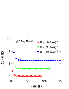
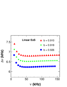
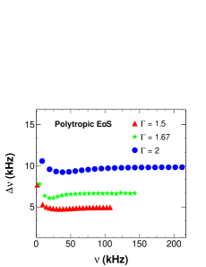
Figure 11: Variation of radial oscillation frequency differences between consecutive modes with the mode frequency $\nu_{n}$ for the (a) MIT Bag Model EoS [left plot], (b) linear EoS [middle plot] and (c) polytropic EoS [right plot].

significantly. Again, for each value of constant $B$, the separation between two consecutive modes decreases towards higher order modes. Thus this separation is maximum for the $f$-mode, followed by lower order $p$-modes. For values of $B$ lying in between $(190\,\mbox{MeV})^{4}$ and $(243\,\mbox{MeV})^{4}$, the intermediate values of the oscillation frequencies are acquired. Similar behaviours of oscillation frequencies are obtained for linear EoS with three values of linear constants: $b=0.910$, $b=0.918$ and $b=0.926$, which is shown in the middle plot of Fig. 11. However, in this case for the larger value of linear constant, i.e. for $b=0.926$, the frequency differences are found to be smaller than that for the other two smaller values of $b$. For the lowest value of $b$, i.e. for $b=0.910$, we get highest values of frequency differences and $b=0.918$ gives the intermediate values. For each values of $b$ considered here, the separation between the consecutive modes is maximum for $f$-mode and is gradually getting smaller for higher order modes. Same study is made for the polytropic EoS with polytropic exponent $1.5$, $1.67$ and $2$, which are shown in the right plot of Fig. 11. Among these considered values of polytropic exponent, we have obtained maximum oscillation frequency differences for $\Gamma=2$. Similar to the other EoSs, for this model also the frequency differences are getting smaller for higher order modes. However for $\Gamma=1.67$ a slight variation in the pattern is observed than that for the other two considered values. Like MIT Bag model EoS, for this EoS also, we have obtained that, larger is the value of $\Gamma$ higher is the oscillation frequency differences.

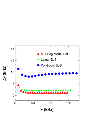
Figure 12: Comparison of frequency differences between consecutive modes with respect to the mode frequency for all three EoSs with the model parameters for which respective EoSs are giving maximum oscillation frequencies.

In Fig. 12, a comparison between these EoSs are made. The frequency differences for linear and MIT Bag model EoSs are decreasing gradually with increasing frequencies. For polytropic EoS, the pattern is slightly distorted as shown in figure. Maximum values of frequency differences are observed for polytropic EoS with $\Gamma=2$, whereas minimum differences are observed for MIT Bag model EoS with $B=(243\,\mbox{MeV})^{4}$ but these are comparable to that of linear EoS with $b=0.910$. Thus it is clear that, the radial oscillation frequencies of SSs crucially depend on the model and the model parameters used.

V.2 GWE frequencies of SSs

Table 3: GWE frequencies in kHz from SSs for three EoSs with different model parameters.

EoSs	Model	Echo	GWE	GWE
	Parameter	time (ms)	Frequency (kHz)	Repetition Frequency (kHz)
MIT Bag model	$B=(190\,\mbox{MeV})^{4}$	0.078	39.91	6.35
	$B=(217\,\mbox{MeV})^{4}$	0.060	51.70	8.23
	$B=(243\,\mbox{MeV})^{4}$	0.048	64.98	10.34
Linear EoS	$b=0.910$	0.043	72.90	11.60
	$b=0.918$	0.044	70.21	11.18
	$b=0.926$	0.046	67.42	10.73

The GWE frequencies of different SS models are given in Table 3. The possible SS models which fulfil the criterion for emitting GWE frequencies, i.e. featuring a photon sphere and the radius not exceeding the Buchdahl’s limit radius are shown in Fig. 1. So, the EoSs are chosen in order to obtain maximum mass ranges of the stellar configuration. Along with the two models as shown in the Fig. 1, which have the required compactness, we have chosen four other EoSs by varying the model parameter of MIT Bag model and linear EoS. For MIT Bag model [Eq. (1)] with $B={(190\,\mbox{MeV})}^{4},{(217\,\mbox{MeV})}^{4}$ and ${(243\,\mbox{MeV})}^{4}$, and linear EoS [Eq. (2)] with $b=0.910,0.918$ and $0.926$, the compactness within the range of $0.33$ to $0.44$ can be obtained. So we have calculated GWE frequencies in these models.

     

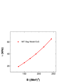
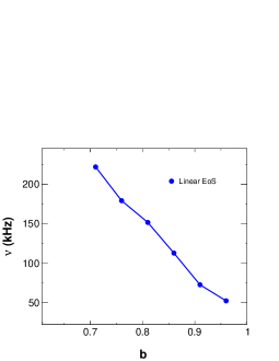
Figure 13: Variation of GWE frequencies with different model parameters: left plot is for MIT Bag model with different Bag constant $B$ and right plot is for linear EoS with linear constant $b$.

Here we report the GWE frequencies obtained for three values of Bag constant $B$: $(190\,\mbox{MeV})^{4}$, $(217\,\mbox{MeV})^{4}$ and $(243\,\mbox{MeV})^{4}$ and three values of linear constant $b$: $0.910$, $0.918$ and $0.926$. These considered EoSs lead to different types of SSs with varying maximum masses. For MIT Bag model, the maximum masses are $M_{max}\approx 3.29\,M_{\odot}$ with $B=(190\,\mbox{MeV})^{4}$, $M_{max}\approx 2.54\,M_{\odot}$ with $B=(217\,\mbox{MeV})^{4}$ and $M_{max}\approx 2.02\,M_{\odot}$ with $B=(243\,\mbox{MeV})^{4}$. The linear EoS leads to maximum masses $M_{max}\approx 1.77\,M_{\odot}$ for $b=0.910$, $M_{max}\approx 1.84\,M_{\odot}$ for $b=0.918$ and $M_{max}\approx 1.92\,M_{\odot}$ for $b=0.926$. Thus, it is seen that with the increasing value of $B$ of MIT Bag model EoS, the maximum mass of SS decreases, whereas it increases with the increasing value of $b$ of linear EoS. Our result shows that the GWE frequency increases with increase in values of Bag constant $B$. For $B={(190\,\mbox{MeV})}^{4}$, the GWE frequency is $\omega_{MIT,\,echo}=39.91$ kHz which is much smaller than the values corresponding to $B={(217\,\mbox{MeV})}^{4}$ and ${(243\,\mbox{MeV})}^{4}$, which also show a large difference ($\sim 13.28$ kHz). Thus GWE frequencies for these SS models show a large variation in their values. For linear EoSs, with $b=0.910$, maximum echo frequency of $72.90$ kHz is observed. For $b=0.918$, the echo frequency is $\approx 67.42$ kHz, which is near to the value of $\omega_{MIT,\,echo}$ with $B={(243\,\mbox{MeV})}^{4}$. The echo frequency for polytropic EoS is not observed as the required compact SSs are not found for such type of EoSs. Along with the characteristic echo frequencies the repetition frequencies of GWEs are also calculated (shown in Table 3 ). The repetition frequencies are found to be much smaller than the GWE frequencies and they are following the same pattern as the corresponding echo frequencies.

Further, for more clarity the variation of GWE frequencies with different model patrameters for MIT Bag model and linear EoSs are shown in Fig. 13. The first plot of this figure shows that, with increasing value of Bag constant $B$, GWE frequency increases. Whereas from the second plot it is clear that unlike MIT Bag model, GWE frequency decreases with the increasing value of linear constant $b$.

VI Summary and Conclusions

In the first part of this study, we have computed frequencies of 22 lowest radial oscillation modes and in the second part, we have computed the echo frequencies of SSs considering that the fluid pressure follows certain EoSs. Considering isotropic configuration of strange matter, we have integrated the TOV equations in general relativistic case numerically to get the values of mass, radius of the star and the metric term. For the defined pressure-energy density relations, we have obtained different SS configurations. After that, the radial and pressure perturbation equations respectively in $\xi=\Delta r/r$ and $\eta=\Delta p/p$ are solved for the eigenfrequencies. To calculate echo frequencies those stars are chosen which can echo GWs by requiring the condition for compactness. The typical echo time is then calculated and the characteristic GWE frequencies along with the repetition frequencies are determined for linear and MIT Bag model EoSs.

In this study of radial oscillation modes of SSs, we have calculated the respective $f$-mode and $p$-modes of oscillation frequencies associated with different SSs. The characteristic echo frequencies and the respective repetition of the echo frequencies are also calculated for SSs. Table 2 and Table 3 summarise the results of the work. From the numerical results we can summarise our work as follows.

The amplitude of radial perturbations $\xi_{n}(r)$ is larger closer to the centre and much smaller near the surface for all the three EoSs. For all mode of frequencies the maximum amplitude of $\xi_{n}(r)$ is same. The pressure perturbation $\eta_{n}(r)$ is larger closer to the centre and near the surface of the star for MIT Bag model, linear EoS and polytropic EoS. The values of $\xi_{n}(r)$ and $\eta_{n}(r)$ are differing from model to model and also for parameters of the models.

Polytropic EoS gives the largest value of radial frequencies among the three EoSs. MIT Bag model and linear EoSs have nearer values of radial frequencies. With increasing modes, the frequencies also increases. The separation between two consecutive oscillation modes decreases with the increase in frequency or mode for all three EoSs. However, this effect is less pronounced for higher order modes. Moreover, the frequency differences for polytropic EoS have shown a slight distortion. Further, the magnitude of this frequency separation depends upon the EoS as well as on the associated model parameter. Among all three EoSs the polytropic EoS with $\Gamma=2$ gives the maximum separation. Thus from these results, it is clear that oscillation frequencies show high dependency on model and model parameters.

In case of GWE frequency not all EoSs are able to emit echo. Those EoSs which give stellar configuration with much higher compactness are able to give echo frequencies. The echo frequency obtained for MIT bag model and linear EoSs show a distinct variation in their values depending on the model parameters. Thus it can be said that, the calculated characteristic echo frequencies as well as repetition frequencies changes with model and model parameters.

The existence of SS has not based on firm footing till now, despite of the possible evidences of SS candidates. As mentioned in above sections, the structure of SS crucially depends on the EoS. Considering some relevant EoSs for such stars one will get different SS configurations. The knowledge of possible SS configurations will help in searching such compact stars. Again from the reflected GWE signal it is also possible to say about the structural behavior of such stars. The prediction of echo signal will get its firm foundation by the experimental detection of such signal using some future generation of GW detectors. We think with a sufficient amount of experimental data on echo frequencies of GWs, it could be possible to constrain the parameters of EoSs and hence to find out the most viable EoS. In this study the echo frequencies of GWs are found to be above 30 kHz range. Advanced LIGO, Advanced Virgo and KAGRA are projected to have sensitive to GWs with frequencies of $\sim$ 20 Hz - 4 kHz and with amplitudes of $\sim 2\times 10^{-22}$ - $4\times 10^{-24}$ strain/$\sqrt{\mbox{Hz}}$ (martynov, ; abbot, ). Due to limited by shot noise at high frequencies, currently LIGO and Virgo observatories have a sensitivity of $\geq 2\times 10^{-23}$ strain/$\sqrt{\mbox{Hz}}$ at $3$ kHz. According to D. Martynov et al. this sensitivity can be enhanced by an optical configuration of detectors using the current interferometer topology to reach $\geq 7\times 10^{-25}$ strain/$\sqrt{\mbox{Hz}}$ at $2.5$ kHz. These proposed instruments with optimal arm length of $\approx 20$ km would have the sensitivity to detect the amount of postmerger neutron star oscillations at per the third generation detectors, such as Cosmic Explorer (CE) (abbott, ) and Einstein Telescope (ET) (punturo, ). The CE is a proposed 40 km arm length L-shaped observatory to deepen the GW view of the cosmos, whose sensitivity may reach below $10^{-25}$ strain/$\sqrt{\mbox{Hz}}$ at above few kHz frequencies. On the other hand, ET is a $10$ km arm length L-shaped underground proposed observatory which will be able to reach the sensitivity of $>3\times 10^{-25}$ strain/$\sqrt{\mbox{Hz}}$ at $100$ Hz and of $\sim 6\times 10^{-24}$ strain/$\sqrt{\mbox{Hz}}$ at $\sim 10$ kHz. It is clear that none of present or near future generation of GW detectors could reach a sensitivity required to detect GWEs in the range of our study. However, in a very recent study by S. L. Danilishin et al. (danilishin, ) shows that by the application of advanced quantum techniques to suppress the quantum noise at high frequency end in the design of GW detectors, the sensitivity of the present GW detectors can be enhanced significantly. So, the application of such techniques to the proposed third generation of detectors mentioned above may lead to increase their sensitivity to our expected level. Otherwise, we have to wait for the distant future, fourth generation GW detectors with sufficiently higher sensitivity in the kHz range of frequencies to test the results of this study. Obviously, a detailed study on the possibility of detection GWE frequencies and ways to increase detector sensitivities can shed more light in this regard in future.

References

- (1) E. Farhi and R. L. Jaffe, Phys. Rev. D 30, 2379 (1984).
- (2) E. Witten, Phys. Rev. D 30, 272 (1984).
- (3) C. Alcock and A. Olinto, Ann. Rev. Nucl. Part. Sci. 38, 161 (1988).
- (4) T. Øvergård and E. Østgaard, Astron. and Astrophys. 243, 412 (1991).
- (5) J. L. Zdunik, Astron. and Astrophys. 394, 641 (2002) [arXiv:astro-ph/0208334].
- (6) A. P. Martnez, R. G. Felipe and D. M. Paret, Inter. J. Mod. Phys. D 19, 1511 (2010) [arXiv:1001.4038].
- (7) F. Weber, M. Orsaria, H. Rodrigues and S. -H. Yang, Proceed. IAU Symp. No. 291, 61 (2012) [arXiv:1210.1910].
- (8) F. Weber, Prog. Part. and Nucl. Phys. 54, 193 (2005) [arXiv:astro-ph/0407155].
- (9) S. L. Shapiro, S. A. Teukolsky, Black hole, white dwarf and neutron stars, The physics of compact objects, WILEY-VCH Verlag GmbH & Co. KGaA, Weinheim (2004).
- (10) G. Handler, Planets, Stars and Stellar Systems, Springer, (2013) [arXiv:1205.6407] .
- (11) S. Chandrasekhar, Astrophys. J. 140, 417 (1964).
- (12) S. Chandrasekhar, Phys. Rev. Let. 12, 114 (1964).
- (13) G. Chanmugam, Astrophs. J. 217, 799 (1977).
- (14) E. N. Glass and L. Lindblom, Astrophys. J. Suppl. Ser. 53, 93 (1983).
- (15) P. Haensel, J. L. Zdunik and R. Schaeffer, Astron. and astrophys. 217, 137(1989).
- (16) B. Datta, P. K. Sahu, J. D. Anand and A. Goyal, Phys. Lett. B 283, 313 (1992) [arXiv:astro-ph/9304024].
- (17) H. M. Váth and G. Chanmugam, Astron. and Astrophys. 260, 250 (1992).
- (18) G. Panotopoulos and I. Lopes, Phys. Rev. D 96, 083013 (2017) [arXiv:1709.06643].
- (19) G. Panotopoulos and I. Lopes, Phys. Rev. D 98, 083001 (2018).
- (20) I. Lopes, G. Panotopoulos and A. Rincón, Eur. Phys. J. Plus 134, 454 (2019) [arXiv:1907.03549].
- (21) F. D. Clemente, M. Mannarelli and F. Tonelli, Phys. Rev. D 101, 103003 (2020) [arXiv:2002.09483].
- (22) V. Ferrari and K. D. Kokkotas, Phys. Rev. D 62, 107504 (2000) [arXiv:gr-qc/0008057].
- (23) P. Pani and V. Ferrari, Class. Quan. Grav. 35, 15LT01 (2018) [arXiv:1804.01444].
- (24) Yu. G. Ignat’ev and A. V. Zakharov, Phys. Lett. 66, 3 (1978).
- (25) J. Abedi, H. Dykaar and N. Afshordi, Phys. Rev. D 96, 082004 (2017) [arXiv:1612.00266].
- (26) J. Abedi and N. Afshordi, JCAP 11, 010 (2019) [arXiv:1803.10454].
- (27) J. Abedi and N. Afshordi, [arXiv:2001.00821] (2020).
- (28) R. S. Conklin, B. Holdom and J. Ren, Phys. Rev. D 98, 044021 (2018) [arXiv:1712.06517 ].
- (29) M. Mannarelli and F. Tonelli, Phys. Rev. D 97, 123010 (2018).
- (30) H. A. Buchdahl, Phys. Rev. 116, 1027 (1959).
- (31) B. Abbott et al., Phys. Rev. Lett. 119, 161101 (2017) [arXiv:1710.05832].
- (32) X.-D. Li, Bombaci I., Dey M., Dey J. and van den Heuvel E. P. J., Phys. Rev. Let. 83, 19 (1999) [arXiv:hep-ph/9905356].
- (33) J. A. Henderson and D. Page, Astrophys. and Space Sci. 308, 513 (2007) [arXiv:astro-ph/0702234].
- (34) P. Haensel, J. L. Zdunik and R. Schaeffer, Astron. and Astrophys. 160, 121 (1986).
- (35) R. Sharma and S. D. Maharaj, Mon. Not. Roy. Astron. Soc. 375, 1265 (2007) [arXiv:gr-qc/0702046].
- (36) A. Chodos et al., Phys. Rev. D 9, 3471 (1974).
- (37) A. Chodos et al., Phys. Rev. D 10, 2599 (1974).
- (38) C. Alcock, E. Farhi and A. Olinto, Astrophys. J. 310, 261 (1986).
- (39) A. Aziz, S. Ray, F. Rahaman, M. Khlopov and B. K. Guha, Inter. J. Mod. Phys. D 28, 1941006 (2019).
- (40) P. A. Carinhas, ApJ 412, 213 (1993).
- (41) M. Dey, I.Bombaci, J. Dey, S. Ray and B. C. Samanta, Phys. Lett. B 438, 123 (1998) [arXiv:astro-ph/9810065].
- (42) D. Gondek-Rosińska , T.Bulik, L. Zdunik, E. Gourgoulhon, S. Ray, J. Dey and M. Dey, Astron. and Astrophys. 363, 1005 (2000) [arXiv:astro-ph/0007004].
- (43) R. F. Tooper, Astrophys. J. 140, 434 (1964).
- (44) R. F. Tooper, Astrophys. J. 142, 1541 (1965).
- (45) S. Thirukkanesh and F. C. Ragel, Pram. J. Phys. 78, 687 (2012).
- (46) L. Herrera and W. Barreto, Gen. Relativ. Gravit. 36, 127 (2004) [arXiv:gr-qc/0309052].
- (47) K. D. Kokkotas and J. Ruoff, Astron. and Astrophys. 366, 565 (2001) [arXiv:gr-qc/0011093].
- (48) S. Ray, M. Malheiro, J. P. S Lemos. and V. T. Zanchin, Braz. J. Phys. 34, 310 (2004) [arXiv:nucl-th/0403056].
- (49) J. M. Lattimer and M. Prakash, From Nuclei to Stars, World Scientific, (2010) [arXiv:1012.3208].
- (50) P. Haensel, A. Y. Potekhin and D. G. Yakovlev Neutron stars 1: Equation of state and structure, Astrophys. Spac. Scin. Lib. 326, (2007).
- (51) R. C. Tolman, Phys. Rev. 55, 364 (1939).
- (52) J. R. Oppenheimer and G. M. Volkoff, Phys. Rev. 55, 374 (1939).
- (53) J. P. Cox. Theory of stellar pulsation, Princeton University Press (1980).
- (54) V. Cardoso and P. Pani, Nat. Astron. 1, 586 (2017) [arXiv:1709.01525].
- (55) Martynov D. et al., Phy. Rev. D 99, 102004 ( 2019).
- (56) B. Abbott et al., Liv. Rev. Rel. 23, 3 ( 2020).
- (57) M. Punturo et al., Class. Quan. Grav. 27, 194002 (2010).
- (58) S. L. Danilishin, F. Y. Khalili and H. Miao, Liv. Rev. Rel. 22, 2 (2019).