Reconstruction in one dimension from unlabeled Euclidean lengths

Abstract

Let $G$ be a $3$-connected graph with $n$ vertices and $m$ edges. Let ${\bf p}$ be a randomly chosen mapping of these $n$ vertices to the integer range $[1..2^{b}]$ for $b\geq m^{2}$. Let ${\bf l}$ be the vector of $m$ Euclidean lengths of $G$’s edges under ${\bf p}$. In this paper, we show that, WHP over ${\bf p}$, we can efficiently reconstruct both $G$ and ${\bf p}$ from ${\bf l}$. In contrast to this average case complexity, this reconstruction problem is NP-HARD in the worst case. In fact, even the labeled version of this problem (reconstructing ${\bf p}$ given both $G$ and ${\bf l}$) is NP-HARD. We also show that our results stand in the presence of small amounts of error in ${\bf l}$, and in the real setting with approximate length measurements.

Our method is based on older ideas that apply lattice reduction to solve certain SUBSET-SUM problems, WHP. We also rely on an algorithm of Seymour that can efficiently reconstruct a graph given an independence oracle for its matroid.

1.  Introduction

Let ${\bf p}$ be a configuration of $n$ points ${\bf p}_{i}$ on the real line. Let $G$ be a graph with $n$ vertices and $m$ edges. For each edge $ij$ in $G$, we denote its Euclidean length as $\ell_{ij}({\bf p}):=|{\bf p}_{i}-{\bf p}_{j}|$. We denote by ${\bf l}=\ell({\bf p})$, the $m$-vector of all of these measured lengths. In a labeled reconstruction problem we assume that $G$ is $2$-connected, we are given $G$ and ${\bf l}$, and we are asked to reconstruct ${\bf p}$. In a unlabeled reconstruction problem we assume that $G$ is $3$-connected, we are just given ${\bf l}$ (we are not even given $n$), and we are asked to reconstruct $G$ and ${\bf p}$.

As explained below, when these connectivity conditions are not satisfied, then the reconstruction problems are almost always ill posed, and there will simply not be enough information for any algorithm (efficient or not) to uniquely determine the reconstruction. In the labeled setting, these problems are generally well posed as soon as $G$ is $2$-connected [3]. In the unlabeled setting, these problems are generally well posed as soon as $G$ is $3$-connected [8]. Even when well-posed, and discretely defined, these problems are very hard to solve computationally; indeed, even the labeled problem for integers in one dimension is (strongly) NP-HARD [15].

Two and three dimensional labeled and unlabeled reconstruction problems often arise in settings such as sensor network localization and molecular shape determination. These problems are even harder than the one dimensional setting studied here. But due to the practical importance of these applications, many heuristics have been studied, especially in the labeled setting. There do exist polynomial time algorithms that have guarantees of success, but only on restricted classes of graphs and configurations. For example, labeled problems can be solved with semi-definite programming if the underlying graph-configuration-pair happens to be "universally rigid" [18]. Labeled problems in $d$-dimensions can be solved with with greedy algorithms if the underlying graph happens to be "$d$-trilateral". This means that the graph has an edge set that allows one to localize one or more $K_{d+2}$ subgraphs, and then iteratively glue vertices onto already-localized subgraphs using $d+1$ edges, (and unambiguously glue together already localized subgraphs) in a way to cover the entire graph. There is also a huge literature on the related problem of low-rank matrix completion. Typically, those results assume randomness in choice of matrix sample locations, roughly corresponding to the graph $G$ in our setting.

Unlabeled problems are much harder, with fewer viable approaches. When the underlying graph happens to be "$d$-trilateral"  [9, 6]. then an unlabeled problem in $d\geq 2$ can be solved with using a combinatorial search in $O(m^{k})$ time, where $k$ is a large fixed exponent for each dimension [9, 6]. (In one dimension, it is actually required that the graph is $2$-trilateral, instead of $1$-trilateral in order for this to work [6] .)

The unlabeled reconstruction problem in the one dimensional integer setting also goes by names such as “the turnpike problem” and the “partial digest problem”. Theoretical work on these problems has typically been worst case analysis and often only apply to the complete graph (e.g. [11, 17, 2]).

In this paper we present an algorithm that can provably solve the one dimensional unlabeled (and thus, also the labeled) reconstruction problems in polynomial time, for each fixed, appropriately minimally connected graph, WHP over random ${\bf p}$ as long as we have sufficient accuracy of the length measurements. The algorithm is based on combining the LLL lattice reduction algorithm [12, 10, 4] together with the graphical matroid reconstruction algorithm of Seymour [16]. The limiting factor of our algorithm in practice is its reliance on having sufficient bits of accuracy in the measurements of ${\bf l}$. But the existence of such an efficient algorithm with these theoretical guarantees was surprising to us. Even though the required precision grows with the number of edges, we give an explicit bound. This is in contrast with theoretical results about generic configurations often found in rigidity theory, which are non quantitative in an integer setting or in the presence of noise.

1.1.  Connectivity assumption

Labeled setting:

Clearly we can never detect a translation or reflection of ${\bf p}$ in the line, so we will only be interested in recovery of the configuration up to such congruence.

In the labeled setting, if $i$ is a cut vertex of $G$, then we can reflect the positions of one of the cut components across ${\bf p}_{i}$ without changing ${\bf l}$. Such a flip is invisible to our input data. To avoid such partial reflections, we must assume that $G$ is $2$-connected.

For more information about when labeled reconstruction problems are generally well posed in the real setting, in $2$ and higher dimensions, see [3, 7].

(a)	(b)	(c)	(d)

Figure 1: The $2$-swap operation. The graphs, (a) and (d) are 2-isomorphic but not isomorphic. Note that the edge lengths are unchanged under a 2-isomorphism.

Unlabeled Setting:

In the unlabeled setting, we can never detect a renumbering of the points in ${\bf p}$ along with a corresponding vertex renumbering in $G$, so we will be unconcerned with such isomorphic outputs.

In the unlabeled setting, if $i$ is a cut vertex of $G$, then we can cut the vertex set at $i$ and then glue back one of the cut components at a different vertex completely (with its points in one of two orientations) without changing ${\bf l}$. Next, suppose $i,j$ form a vertex cut set of $G$, then we can cut $G$ at $i$ and $j$ and then glue back one of the components in reverse (See Figure 1) without changing ${\bf l}$. To avoid such swapping, we must assume that $G$ is $3$-connected.

For more information about when unlabeled reconstruction problems are generally well posed in the real setting, in $2$ and higher dimensions, see [8, 6].

1.2.  Integer setting

Moving to an algorithmic setting, we will now assume that the points are placed at integer locations in the set $[1...B]$, with $B=2^{b}$ for some $b$. For the labeled problem, we will want an algorithm that takes as input $G$ and integer vector ${\bf l}$, and outputs ${\bf p}$ (up to congruence). For the unlabeled problem, we will want an algorithm that takes as input the integer vector ${\bf l}$, and outputs $G$ (up to vertex labeling) and ${\bf p}$ (up to congruence).

Even the labeled problem is strongly NP-HARD by a result of Saxe [15]. Interestingly, one of his reductions is from SUBSET-SUM. This is a problem that, while hard in the worst case, can be efficiently solved, using the Lenstra-Lenstra-Lovász (LLL) lattice reduction algorithm [12], for most instances that have sufficiently large integers [10]. Indeed, we will take cue from this insight and use LLL to solve both the labeled and unlabeled reconstruction problems.

We say that a sequence, $A_{m}$, of events in a probability space occurs with high probability as $m\to\infty$ (WHP) if $\Pr[A_{m}]=1-o(1)$. Here is our basic result.

Theorem 1.1.

Let $G$ be a $3$-connected (resp. $2$-connected) graph. Let $b\geq m^{2}$. Let each ${\bf p}_{i}$ be chosen uniformly and randomly in $[1..2^{b}]$. Then there is a polynomial time algorithm that succeeds, WHP, on the unlabeled (resp. labeled) reconstruction problems.

Both the success probability and the convergence rate can be estimated more explicitly (see below). However, what we can prove seems to be pessimistic, especially if we have some extra information about the number of vertices. Experiments (see below) show that our algorithm succeeds with very high probability on randomly chosen ${\bf p}$ even with significantly fewer bits. In part, this is because the LLL algorithm very often outperforms its worst case behavior [13] on random input lattices.

1.3.  Errors in input

To move towards a numerical setting, we need to differentiate between the geometric data in ${\bf p}$ and its combinatorial sign data. The combinatorial sign data, will be represented by an orientation $\sigma_{\bf p}$ (see definitions below), which represents, for each edge, which vertex is to left side and which is on right side in the configuration ${\bf p}$. We will say that a reconstruction algorithm succeeds combinatorially if it correctly outputs $G$ and $\sigma_{\bf p}$. Once we have the correct combinatorial data, we can simply apply a linear least squares algorithm to get a good estimate of ${\bf p}$.

To model error we consider the case where there may be $\{-1,0,1\}$ error, added adversarially, to each of the $\ell_{ij}$ integer measurements.

Theorem 1.2.

Let $G$ be a (sufficiently connected) graph. Let $b\geq m^{2}$. Let each ${\bf p}_{i}$ be chosen uniformly and randomly in $[1..2^{b}]$. Then, in both the labeled and unlabeled settings, there is a polynomial time algorithm that, WHP, combinatorially succeeds on the noisy reconstruction problems.

Failure modes of our algorithm are discuss in Section 4.

1.4.  Real setting

Theorem 1.2 can be used in the setting where ${\bf p}$ is not integral to begin with, but rather is real valued, and with each ${\bf p}_{i}$ in the real-range $[1..B]$, with uniform probability. In this case our ${\bf l}$ is not integral either, but we can simply round it to the nearest integer, giving us ${\bf l}^{\prime}$. This ${\bf l}^{\prime}$ will, in fact, be a $\{-1,0,1\}$ noisy version of the lengths obtain from ${\bf p}^{\prime}$, the configuration where ${\bf p}$ has been rounded to the integers. Hence, our noisy theorem applies to this integer input.

Since we are rounding to the nearest integer over ${\bf l}$, and our values have the range $[1..B]$, this essentially means that we are requiring $b$-bits of measurement accuracy in our real valued measured ${\bf l}$.

1.5.  Basic ideas

Consider a simple cycle in $G$, thought of an cyclic ordered list of vertices. As we walk along this cycle in ${\bf p}$, some of the edges go to the right and some to the left. If we sum up the Euclidean lengths of these edges, with a appropriate sign, determined by the vertex ordering on the line, and denoted by $\sigma_{\bf p}$, the sum must equal $0$, since the cycle closes up. Thus, these $\pm 1$s must form a "small-integer" relation on length vector ${\bf l}$. Indeed there is such a small integer relation on ${\bf l}$ corresponding to any cycle in $G$. These cycle relations will form a linear space $S^{\sigma_{{\bf p}}}$ of linear relations on ${\bf l}$, of dimension $c:=m-n+1$ (the dimension of the cycle space of $G$).

On the other hand, suppose our ${\bf p}_{i}$ have been chosen uniformly and randomly from a set of sufficiently large integers. Then we should not expect there to be any other "accidental" small integer relations on ${\bf l}$, that are not in $S^{\sigma_{{\bf p}}}$.

The problem of finding the smallest integer relations on ${\bf l}$ is NP-HARD. Fortunately, the LLL basis-reduction algorithm can be used to find, in polynomial time (and acceptably fast in practice), a basis of integer relations that are within a factor of $2^{(m-1)/2}$ of the smallest such basis. This factor may turn our small relations in $S^{\sigma_{{\bf p}}}$ to "medium sized" integer relations on ${\bf l}$. But when starting with sufficiently large integers, we still do not expect there to be any other accidental medium sized integer relations on ${\bf l}$ that are not in $S^{\sigma_{{\bf p}}}$. Thus by using LLL, we can recover the space $S^{\sigma_{{\bf p}}}$, WHP.

This is exactly the approach discovered by Lagarias and Odylyzko [10] to solve knapsack problems WHP, over sufficiently large integer inputs. A simpler analysis of this method is described by Frieze [4], which we will build upon here. Recently in  [22, 5], this exact same approach has been carefully applied to recover an unknown discrete signal from multiple large integer linear measurements. (The case of multiple measurements is also briefly suggested at the end of [4]). As described by [22], this approach can even work in the presence of sufficiently small amounts of noise. We will only deal with constant sized noise in our setting. Indeed, as shown in [22], the optimal algorithm should always truncate enough bits, so that the noise is effectively constant sized.

The main difference between our setting and that of [10] and [22], is that in our case, we are looking for $c$ linearly independent small/medium relations in one random data vector, instead of just a single relation in one or more random data vectors. Another technical difference we will need to deal with explicitly, is that our probability statements are over random generating ${\bf p}$, instead of random data vectors ${\bf l}$. And in particular, our the process going from ${\bf p}$ to ${\bf l}$ has an absolute value, making it not quite linear.

Once we recover $S^{\sigma_{{\bf p}}}$, our next task is use this space to recover the graph $G$. For this, we will use a polynomial time algorithm of Seymour [16] that is able to construct a graph when given an efficient "matroid oracle" (ie. a cycle detector). We show below how we can use a matrix representation of $S^{\sigma_{{\bf p}}}$ to implement such a matroid oracle for $G$.

Once we have $G$, our next task is to use $G$ and $S^{\sigma_{{\bf p}}}$ together to compute $\sigma_{{\bf p}}$ itself. This can be done, by iterating over simple cycles in $G$ to greedily determine the left/right orientation of its edges in ${\bf p}$.

Finally, we can use $G$, $\sigma_{{\bf p}}$ and ${\bf l}$ to determine the positions of each of the ${\bf p}_{i}$. In the noiseless case, this can be done by traversing a spanning tree of $G$ and laying out the points. In the noisy case, this step can be solved as a least squared problem.

input : ${\bf l}$

output : ($G$, ${\bf p}$)

1 $S^{\sigma_{{\bf p}}}\leftarrow$ ComputeRelations(${\bf l}$);

2 $G\leftarrow$ Seymour($S^{\sigma_{{\bf p}}}$);

3 $\sigma_{\bf p}\leftarrow$ ComputeOrientation($G$, $S^{\sigma_{{\bf p}}}$);

4 ${\bf p}\leftarrow$ Layout($G$, $\sigma_{\bf p}$, ${\bf l}$);

5 return ($G$,${\bf p}$);

Algorithm 1 The full Algorithm

2.  Graph theoretic preliminaries

First we set up some graph-theoretic background.

2.1.  Graphs, orientations, and measurements

In this paper, $G=(V,E)$ will denote a simple, undirected graph with $n$ vertices and $m$ edges. For a natural number $n\in\mathbb{N}$, define the notation $[n]:=\{1,\ldots,n\}$. We will need to associate vertices and edges with columns and rows of matrices, so, for convenience we fix bijections between $V$ and $[n]$ and $E$ and $[m]$.

Definition 2.1.

Let $G=(V,E)$ be an undirected simple graph with $n$ vertices and $m$ edges. We denote undirected edges by $\{i,j\}$, with $i,j\in V$.

An orientation $\sigma$ of $G$ is a map that assigns each undirected edge $\{i,j\}$ of $G$ to exactly one of the directed edges $(i,j)$ or $(j,i)$; i.e., $\sigma(\{i,j\})\in\{(i,j),(j,i)\}$. Informally, $\sigma$ assigns one endpoint of each edge to be the tail and the other to be the head.

An oriented graph $G^{\sigma}$ is a directed graph obtained from an undirected graph $G$ and an orientation $\sigma$ of $G$ by replacing each undirected edge $\{i,j\}$ of $G$ with $\sigma(\{i,j\})$.

We are usually interested in a pair $(G,{\bf p})$ where $G$ has $n$ vertices and ${\bf p}$ is a configuration of $n$ points $({\bf p}_{1},\ldots,{\bf p}_{n})$ on the line. Such a pair has a natural ordering of $G$ associated with it:

Definition 2.2.

Let $(G,{\bf p})$ denote a graph with $n$ vertices and ${\bf p}$ a configuration of $n$ points. Define the configuration orientation $\sigma_{\bf p}$ by

$$\sigma_{\bf p}(\{i,j\})=\begin{cases}(i,j)&\text{if ${\bf p}_{i}<{\bf p}_{j}$}\\ (j,i)&\text{otherwise}\end{cases}\qquad\text{(for all $\{i,j\}\in E$)}$$

We say that an orientation $\sigma$ of $G$ is vertex consistent if $\sigma=\sigma_{\bf p}$ for some configuration ${\bf p}$.

There are $2^{m}$ possible orientations, but many fewer are vertex consistent:

Lemma 2.3.

Let $G$ be a graph with $n$ vertices. There are at most $n!$ vertex consistent orientations of $G$.

Proof.

The orientation $\sigma_{\bf p}$ is completely determined by the permutation of $\{1,\ldots,n\}$ induced by the ordering of the ${\bf p}_{i}$ on the line. ∎

Definition 2.4.

Let $G$ be a graph with $n$ vertices and $m$ edges. For $i\neq j$, both in $V$, a signed edge incidence vector $e_{(i,j)}$ has $n$ coordinates indexed by $V$; all the entries are zero except for the $i$th, which is $-1$ and the $j$th, which is $+1$. (So that $e_{(i,j)}=-e_{(j,i)})$.

Given a graph $G$ and an orientation $\sigma$ of $G$, the signed edge incidence matrix $M^{\sigma}(G)$ has as its rows the vectors $e_{\sigma(\{i,j\})}$, over all of the edges $\{i,j\}$ of $G$.

Let $\rho$ be a simple cycle in $G$. A signed cycle vector ${\bf w}_{\rho,\sigma}$ of $\rho$ in $G^{\sigma}$ has $m$ coordinates indexed by $E$. Coordinates corresponding to edges not in $\rho$ are zero. Fixing a traversal order of $\rho$, for an edge $\{i,j\}$ of $\rho$ the $\{i,j\}$th entry of the vector is $1$ if the traversal agrees with $\sigma(\{i,j\})$ and $-1$ if the traversal disagrees. (Signed cycle vectors are not unique, since multiplication by $-1$ will produce the vector associated with traversing the cycle in the other direction.)

If we have fixed some ${\bf p}$, we can shorten ${\bf w}_{\rho,\sigma_{{\bf p}}}$ to ${\bf w}_{\rho}$ (with no explicit orientation written).

A basic fact is:

Proposition 2.5 (see e.g, [14, Chapter 5]).

Let $G$ be a connected graph with $n$ vertices and $m$ edges and $\sigma$ an orientation of $G$. The cokernel of $M^{\sigma}(G)$ over $\mathbb{R}$ has dimension $c:=m-n+1$ and is spanned by signed cycle vectors of simple cycles in $G$.

Definition 2.6.

Let $G$ be a graph and $\sigma$ an orientation of $G$. The signed cycle space $S^{\sigma}$ is the cokernel of $M^{\sigma}(G)$. We can form a basis for $S^{\sigma}$ where each of the $c$ basis vectors is the cycle vector of a simple cycle of $G$. We call such a collection of simple cycles, a cycle basis of $G^{\sigma}$. The cycle vectors of such a cycle basis will remain a basis under any orientation $\sigma$. Thus we can also call such a collection of simple cycles: a cycle basis of $G$.

Note that if we flip the orientations of all of the edges, then the signed cycle space does not change.

With this terminology, we can now describe a family of linear maps related to edge length measurements.

Definition 2.7.

Let $G$ be a graph with $n$ vertices and $\sigma$ and orientation of $G$. We define the oriented measurement map $\ell_{\sigma}:\mathbb{R}^{n}\to\mathbb{R}^{m}$ by

$$\ell_{\sigma}({\bf p})_{\{i,j\}}:=\begin{cases}{\bf p}_{j}-{\bf p}_{i}&\text{if $\sigma(\{i,j\})=(i,j)$}\\ {\bf p}_{i}-{\bf p}_{i}&\text{if $\sigma(\{j,i\})=(j,i)$}\end{cases}$$

For any choice of $\sigma$, $\ell_{\sigma}$ is a linear map.

We also define the measurement map $\ell$ by

$$\ell({\bf p})_{\{i,j\}}=|{\bf p}_{j}-{\bf p}_{i}|$$

The measurement map is only piecewise linear.

This next lemma follows from direct computation.

Lemma 2.8.

Let $(G,{\bf p})$ be a graph and a configuration. Then

$$\ell_{\sigma_{\bf p}}({\bf p})_{\{i,j\}}=|{\bf p}_{j}-{\bf p}_{i}|$$

for all edges $\{i,j\}$ of $G$. In other words, $\ell_{\sigma_{\bf p}}({\bf p})=\ell({\bf p})$.

As a consequence, we get

Lemma 2.9.

Let $(G,{\bf p})$ be a graph with $n$ vertices and ${\bf p}$ a configuration of $n$ points. Then

$$M^{\sigma}(G){\bf p} = \ell_{\sigma}({\bf p})$$

$$M^{\sigma_{\bf p}}(G){\bf p} = \ell({\bf p})$$

Proof.

We directly compute that $M^{\sigma}(G){\bf p}=\ell_{\sigma}({\bf p})$. For the second line, from Lemma 2.8, $\ell({\bf p})=\ell_{\sigma_{{\bf p}}}({\bf p})$. ∎

Lemma 2.10.

Let $(G,{\bf p})$ be a graph with $n$ vertices and ${\bf p}$ a configuration of $n$ points. Let $\rho$ be a simple cycle of $G$. Let ${\bf w}_{\rho}$ be its signed cycle vector in $G^{\sigma_{\bf p}}$. Then

$${\bf w}^{T}_{\rho}\ell({\bf p}) = 0$$

Proof.

By Lemma 2.9, $\ell({\bf p})$ is in the column span of $M^{\sigma_{{\bf p}}}$. By Proposition 2.5, ${\bf w}^{T}_{\rho}={\bf w}^{T}_{\rho,\sigma_{\bf p}}$ annihilates the column span of $M^{\sigma_{{\bf p}}}$. ∎

3.  The algorithm

In this section we describe the algorithm in detail and develop the tools required for its analysis. We will focus on the harder, unlabeled setting, and afterwards describe the various simplifications the can be applied in the labeled case.

3.1.  The sampling model

The algorithm has the following parameters. We have a precision $b\in\mathbb{N}$. There is fixed graph $G$ with $n$ vertices and $m$ edges.

Our algorithm takes as input ${\bf l}=\ell({\bf p})+\varepsilon$, where ${\bf p}$ is selected uniformly at random among configurations of $n$ points with coordinates in $\{1,\ldots,2^{b}\}$ (i.e., $b$-bit integers) and $\varepsilon$ is an error vector in $\{-1,0,1\}^{m}$.

The algorithm does not have access to $n$, only $m$ (via the number of coordinates in ${\bf l}$). All the probability statements are taken with respect to ${\bf p}$, which is not part of the input. This complicates the probabilistic analysis a little bit, relative to [10, 4], but much remains similar.

3.2.  Reconstruct $S^{\sigma_{\bf p}}$

In this section, we will show how, WHP, to reconstruct $S^{\sigma_{\bf p}}$ from ${\bf l}$. Our main tool will be the LLL algorithm [12], as used by [10], and analyzed by [4].

Definition 3.1.

For any vector ${\bf r}$ in $\mathbb{Z}^{m}$ define the lattice $\operatorname{Lat}({\bf r})$ of in $\mathbb{Z}^{m+1}$ as the integer span of the columns of the following $(m+1)$-by-$m$ matrix

$$\operatorname{Lat}({\bf r}):=\begin{pmatrix}{\bf I}_{m}\\ {\bf r}^{T}\end{pmatrix}$$

where ${\bf I}_{m}$ is the $m\times m$ identity matrix.

Remark 3.2.

Frieze [4] multiplies the last row of $\operatorname{Lat}({\bf r})$ by a large constant. We do not do that, so we can easily deal with noise.

In our algorithm we will work over the lattice $\operatorname{Lat}({\bf l})$, where ${\bf l}$ is our noisy length measurement vector.

input : ${\bf l}$

output : $S^{\sigma_{{\bf p}}}$

1 $m\leftarrow|{\bf l}|$;

2 $\Lambda\leftarrow$ LLL($\operatorname{Lat}({\bf l}$));

3 basis $\leftarrow$ threshold($\Lambda$,$\sqrt{2m}2^{m/2}$);

4 $S^{\sigma_{{\bf p}}}\leftarrow$ truncate(basis);

5 return ($S^{\sigma_{{\bf p}}}$);

Algorithm 2 The ComputeRelations Algorithm

Lemma 3.3.

Any vector $\hat{{\bf x}}:=[{\bf x};f]$ in $\mathbb{Z}^{m+1}$ is in $\operatorname{Lat}({\bf r})$ iff we have $f={\bf r}^{T}{\bf x}$.

We use the ";" symbol to denote vertical concatenation.

Proof.

$\hat{{\bf x}}=L{\bf x}$. ∎

Definition 3.4.

Let $G$ be a fixed graph. A configuration ${\bf p}$ determines the orientation $\sigma_{\bf p}$ and then the orientation $G^{\sigma_{\bf p}}$ of $G$. We will use $\rho$ to denote a simple cycle in $G$. For any such cycle $\rho$, let ${\bf w}_{\rho}$ be its signed cycle vector in $G^{\sigma_{\bf p}}$ consisting of coefficients in entries in $\{-1,0,1\}$. Recall that the signs in ${\bf w}_{\rho}$ are determined by $\sigma_{\bf p}$.

Lemma 3.5.

$[{\bf w}_{\rho};0]\in\mathbb{Z}^{m+1}$ is in $\operatorname{Lat}(\ell({\bf p}))$.

Let $\varepsilon$ be a $\{-1,0,1\}^{m}$ be a fixed noise vector, and let ${\bf l}:=\ell({\bf p})+\varepsilon$. Then $\hat{{\bf w}}_{\rho}:=[{\bf w}_{\rho};e_{\rho}]$ is in $\operatorname{Lat}({\bf l})$ where $e_{\rho}:={\bf l}^{T}{\bf w}_{\rho}=\varepsilon^{T}{\bf w}_{\rho}$.

Proof.

This follows from Lemmas 2.10 and 3.3. ∎

Lemma 3.6.

We have $\|\hat{{\bf w}}_{\rho}\|_{2}\leq\sqrt{2n}$.

Proof.

Since ${\bf w}_{\rho}$ is the signed cycle vector of a simple cycle, it has at most $n$ non-zero $\pm 1$ entries. Hence $\|\hat{{\bf w}}_{\rho}\|^{2}_{2}=\|w_{\rho}\|^{2}_{2}+|e_{\rho}|^{2}\leq 2n$. ∎

Definition 3.7.

Let us fix a cycle basis for $G$. This gives us a collection $c:=m-n+1$ linearly independent ${\bf w}_{\rho}$ that span $S^{\sigma_{\bf p}}$ (See Proposition 2.5 and Definition 2.6). This also gives us a corresponding collection of $c$ linearly independent $\hat{{\bf w}}_{\rho}$ vectors. If we take the space spanned by these $\hat{{\bf w}}_{\rho}$ and truncate the $m+1$st coordinate, we obtain the space $S^{\sigma_{\bf p}}$.

Combined with Lemmas 3.5 and 3.6 we obtain:

Lemma 3.8.

$\operatorname{Lat}({\bf l})$ contains at least $c:m-n+1$ linearly independent, integer vectors each of norm at most $\sqrt{2n}$.

Definition 3.9.

Let us run the LLL integer basis reduction algorithm on $\operatorname{Lat}({\bf l})$. The LLL algorithm takes in $\operatorname{Lat}({\bf l})$ and outputs, in polynomial time, an integer basis for $\operatorname{Lat}({\bf l})$ that is “not too large”. Let us call the output basis $\Lambda$.

Lemma 3.10.

$\Lambda$ contains contains at least $c$ linearly independent, integer vectors each of norm at most $\sqrt{2n}2^{m/2}$.

Proof.

Let $\hat{{\bf x}}_{1}...\hat{{\bf x}}_{c}$ be any set of $c$ linearly independent vectors in $\operatorname{Lat}({\bf l})$. Let $M:=\max_{i}||\hat{{\bf x}}_{i}||$. Under the LLL algorithm [12, Proposition 1.12], the norms of the $c$ smallest vectors in $\Lambda$ are bounded above by $2^{(m-1)/2}M$. We simplify $m-1$ to $m$. Meanwhile we can make $M\leq\sqrt{2n}$ using Lemma 3.8. ∎

Since we don’t know $c$ in advance, We will argue that for sufficiently large $b$ then, WHP over ${\bf p}$, for any $\varepsilon$, we have that any vector in $\operatorname{Lat}(\ell({\bf p})+\varepsilon)$ of norm $\leq\sqrt{2m}2^{m/2}$ must be in the space spanned by our $c$ vectors: $\hat{{\bf w}}_{\rho}$. We call any vector of this size or less, medium sized. (We replace $\sqrt{2n}2^{m/2}$ by $\sqrt{2m}2^{m/2}$ since the latter is something the algorithm knows, so we can use it as a threshold.) If this happens, then we can recover $S^{\sigma_{\bf p}}$ (the space spanned by our ${\bf w}_{\rho}$ vectors) from $\Lambda$ by simply taking the linear span of the vectors in $\Lambda$ with norm smaller than this threshold, and truncating the $m+1$st coordinate.

To this end, we flip our focus around. Let us fix $\varepsilon$. Let us fix any single vector $\hat{{\bf x}}:=[{\bf x};f]\in\mathbb{Z}^{m+1}$. This next Proposition, which is our main estimate (proven below), bounds the probability, for ${\bf p}$ chosen uniformly at random, that $\hat{{\bf x}}\in\operatorname{Lat}(\ell({\bf p})+\varepsilon)$ and is not in the span of the $\hat{{\bf w}}_{\rho}$.

Proposition 3.11.

Let $\varepsilon$ be fixed. For any fixed $\hat{{\bf x}}$, the probability, over ${\bf p}$, that $\hat{{\bf x}}\in\operatorname{Lat}(\ell({\bf p})+\varepsilon)$ and $\hat{{\bf x}}\not\in span(\hat{{\bf w}}_{\rho})$ is at most $\frac{2^{n}n!}{B}$.

Meanwhile, there is a limited number of medium sized $\hat{{\bf x}}$.

Definition 3.12.

The discrete ball of radius $k$ in $\mathbb{R}^{d}$ is $\mathbb{Z}^{d}\cap\{{\bf x}\in\mathbb{R}^{d}:\|x\|_{2}\leq k\}$. The discrete cube of radius $k$ is the set $\mathbb{Z}^{d}\cap\{{\bf x}\in\mathbb{R}^{d}:\|{\bf x}\|_{\infty}\leq k\}$.

For any given radius, the discrete ball is contained in the discrete cube by the general relation $\|{\bf x}\|_{\infty}\leq\|{\bf x}\|_{2}$.

Lemma 3.13.

The $d$-dimensional discrete ball of radius $k$ has at most $(2k+1)^{d}=(1+\frac{1}{2k})^{d}(2k)^{d}$ $(2k+1)^{d}\leq(3k)^{d}$ points.

Proof.

The cube of radius $k$ has side length $2k$, so it contains $(2k+1)^{d}$ points. Since the size of the discrete cube bounds that of the discrete ball, we are done. ∎

We need the following specific corollary in our analysis of the algorithm.

Corollary 3.14.

The $(m+1)$-dimensional discrete ball of radius $(2m)^{1/2}2^{m/2}$ contains at most $2^{m^{2}/2}2^{O(m\log m)}$ vectors.

Proof.

Apply Lemma 3.13 with $d=m+1$ and $k=(2m)^{1/2}2^{m/2}$ to bound the size of the discrete ball by

$$\left(3(2m)^{1/2}2^{m/2}\right)^{m+1}\leq 2^{\frac{m(m+1)}{2}}2^{\frac{m+1}{2}}3^{(m+1)}m^{\frac{m+1}{2}}=2^{m^{2}/2}2^{O(m\log m)}$$

∎

This $2^{m^{2}/2}$ will ultimately be the dominant term in our bounds.

Lemma 3.15.

The probability, over ${\bf p}$, that there is an $\varepsilon$ and that there is $\hat{{\bf x}}\in\operatorname{Lat}(\ell({\bf p})+\varepsilon)$ where $\hat{{\bf x}}$ is not in the span of the $\hat{{\bf w}}_{\rho}$ and $\|\hat{{\bf x}}\|_{2}\leq(2m)^{1/2}2^{m/2}$ is at most $\frac{2^{m^{2}/2}\;\;2^{O(m\log m)}}{B}$

Proof.

This follows from a union bound over all possible $\hat{{\bf x}}$ (Corollary 3.14) and $3^{m}$ choices for $\varepsilon$. Using Proposition 3.11 we have

$$\frac{2^{m^{2}/2}\;\;2^{O(m\log n)}\;\;3^{m}2^{n}n!}{B}=\frac{2^{m^{2}/2}\;\;2^{O(m\log m)}}{B}$$

∎

This estimate tells us how to pick $b$ to guarantee a high probability of success.

Lemma 3.16.

Let $b\geq(\frac{1}{2}+\delta)m^{2}$ for fixed $\delta>0$. For $m$ sufficiently large (depending on $\delta$), the probability, over ${\bf p}$, that there is an $\varepsilon$ and that there is $\hat{{\bf x}}\in\operatorname{Lat}(\ell({\bf p})+\varepsilon)$ where $\hat{{\bf x}}$ is not in the span of the $\hat{{\bf w}}_{\rho}$ and of medium norm, is at most $\frac{1}{2^{\delta m^{2}/2}}$

Proof.

For sufficiently large $m$, the quantity $2^{m^{2}/2}2^{O(m\log m)}$ is bounded by $2^{(\frac{1}{2}+\frac{\delta}{2})m^{2}}$. The probability of the event in the statement (using Lemma 3.15) is then at most

$$\frac{2^{(\frac{1}{2}+\frac{\delta}{2})m^{2}}}{2^{(\frac{1}{2}+\delta)m^{2}}}=\frac{1}{2^{\delta m^{2}/2}}$$

∎

This completes the analysis of the first step in our algorithm:

Proposition 3.17.

For all $\delta>0$, there is an $M\in\mathbb{N}$ and a polynomial time algorithm that correctly computes, for any $3$-connected graph $G$ with $n$ vertices and $m\geq M$ edges, the space $S^{\sigma_{p}}$ from ${\bf l}$, with probability at least $1-2^{-\delta m^{2}/2}$. Here probabilities are over ${\bf p}$ chosen uniformly among configurations of $n$ integer points from $\{1,\ldots B\}$, where $B=2^{b}$ and $b\geq(\frac{1}{2}+\delta)m^{2}$.

Proof.

By construction, the algorithm returns the medium sized vectors in the basis $\Lambda$, with norm at most $\sqrt{2m}2^{m/2}$.

From Lemma 3.10, the algorithm must return at least $c$ such linearly independent, medium sized vectors.

We have $b\geq(\frac{1}{2}+\delta)m^{2}$ for some $\delta>0$. By Lemma 3.16, with probability at least $1-2^{-\delta m^{2}/2}$, all the returned vectors are in the span of our $\hat{{\bf w}}_{\rho}$, a $c$-dimensional space. Thus, in this case, it must return exactly $c$ vectors, giving us a basis for the $c$-dimensional space spanned by the $\hat{{\bf w}}_{\rho}$. After truncating the $m+1$st coordinate, we must get a basis for $S^{\sigma_{\bf p}}$ (see Definition 3.7).

The LLL algorithm runs in polynomial time [12]. ∎

3.2.1.  Proof of Proposition 3.11

Now we develop the proof of Proposition 3.11. In what follows $G$ and $\varepsilon$ are always fixed. The fact that the map $\ell()$ includes an absolute value complicates the analysis. We will deal with this by enumerating over fixed graph orientations $\sigma$, as $\ell_{\sigma}()$ is a linear map.

Our main tool will be the following simple fact.

Lemma 3.18.

Let $A$ be a $d$-dimensional affine subset of $\mathbb{R}^{m}$. The number of points in the discrete cube $[-1...B]^{m}$ of radius $k$ intersected with $A$ is at most $(B+2)^{d}\leq(2B)^{d}$.

Proof.

Let $C^{m}$ be the discrete cube of the statement. define $C^{d}$ similarly. The projection of $A$ onto the the first $d$ coordinates by forgetting the last $m-d$ coordinates is a bijective (if not, pick a different coordinate subspace), and in particular injective, affine map that sends points in $A\cap C^{m}$ to points $C^{d}$. It follows that $|A\cap C^{m}|\leq|C^{d}|=(B+2)^{d}$. Since $B\geq 2$, then $B+2\leq 2B$. ∎

We use the range $[-1...B]^{m}$ because these are the possible lengths $\ell({\bf p})$ for ${\bf p}$ in $[1..B]^{n}$ with $\{-1,0,1\}$ errors.

Definition 3.19.

Fix $\varepsilon$, $\hat{{\bf x}}$. Fix a vertex consistent orientation $\sigma$. For each $\rho$ in our cycle basis of $G$, recall that ${\bf w}_{\rho,\sigma}$ denotes its signed cycle vector in $G^{\sigma}$. (The orientation $\sigma$ determines the signs in this vector.) This together with $\varepsilon$ then determines $e_{\rho,\sigma}:=\varepsilon^{T}{\bf w}_{\rho,\sigma}$. And we define $\hat{{\bf w}}_{\rho,\sigma}:=[{\bf w}_{\rho,\sigma};e_{\rho,\sigma}]$.

Definition 3.20.

Fix $\varepsilon$, $\hat{{\bf x}}$. Fix a vertex consistent orientation $\sigma$. We say that an ${\bf r}\in[-1..B]^{m}$ is bad with $(\sigma,\hat{{\bf x}})$ if $\hat{{\bf x}}$ is linearly independent of the $\hat{{\bf w}}_{\rho,\sigma}$ (a property that does depend on ${\bf r}$) and if $\hat{{\bf x}}$ and the $\hat{{\bf w}}_{\rho,\sigma}$ are in $\operatorname{Lat}({\bf r})$.

We say that a configuration ${\bf p}$ is sad with $(\sigma,\hat{{\bf x}})$ if ${\bf r}:=\ell_{\sigma}({\bf p})+\varepsilon$ is in $[-1..B]^{m}$ and ${\bf r}$ is bad with $(\sigma,\hat{{\bf x}})$.

We begin by bounding badness and then sadness.

Lemma 3.21.

For any orientation $\sigma$, the set of ${\bf r}$ that are bad with $(\sigma,\hat{{\bf x}})$ lie in an affine subspace $A$ of $\mathbb{R}^{m}$ of dimension $=m-c-1=n-2$.

Proof.

If $\hat{{\bf x}}$ is in the span of the $\hat{{\bf w}}_{\rho,\sigma}$, then no ${\bf r}$ are bad with $(\sigma,\hat{{\bf x}})$, by definition. Otherwise we use Lemma 3.3 and count the number of linear constraints. In particular, starting in $\mathbb{R}^{m}$, we have $c$ (linearly independent) constraints on ${\bf r}$ due to the $\hat{{\bf w}}_{\rho,\sigma}$ and one more (linearly independent) constraint due to $\hat{{\bf x}}$. Meanwhile, we have $c=m-n+1$. ∎

Lemma 3.22.

For any orientation $\sigma$, the number of ${\bf r}$ that are bad with $(\sigma,\hat{{\bf x}})$ is $\leq(2B)^{n-2}$.

Proof.

Use Lemmas 3.18 and 3.21. ∎

Lemma 3.23.

Fix $\sigma$. Let ${\bf r}\in[-1..B]^{m}$. Then the number of configurations ${\bf p}$ with $\ell_{\sigma}({\bf p})+\varepsilon={\bf r}$ is at most $B$.

Proof.

Since $G$ is connected any two configurations mapping to the same ${\bf r}$ through $\ell_{\sigma}(\cdot)$ must be related by translation. There are at most $B$ integer translations that can stay in the configuration range. ∎

Lemma 3.24.

Fix $\sigma$. The number of configurations that are sad with $(\hat{{\bf x}},\sigma)$ is $\leq(2B)^{n-1}$.

Proof.

If a configuration ${\bf p}$ is sad with $(\hat{{\bf x}},\sigma)$, then, by definition, ${\bf r}:=\ell_{\sigma}({\bf p})+\varepsilon$ is in $[-1..B]^{m}$, and ${\bf r}$ is bad with $(\hat{{\bf x}},\sigma)$. The result then follows using Lemmas 3.22 and 3.23. ∎

Definition 3.25.

We say that a configuration ${\bf p}$ is sad with $\hat{{\bf x}}$ if, for some vertex consistent orientation $\sigma$, we have ${\bf p}$ sad for $(\sigma,\hat{{\bf x}})$.

Lemma 3.26.

The number of configurations that are sad with $\hat{{\bf x}}$ is $\leq n!(2B)^{n-1}$.

Proof.

This follows using Lemma 3.24 and counting the number of vertex consistent orientations. ∎

Lemma 3.27.

The probability (over ${\bf p}$) that ${\bf p}$ is sad with $\hat{{\bf x}}$ is at most $\frac{2^{n}n!}{B}$

Proof.

There are $B^{n}$ configurations, as the $n$ points are chosen independently. Then from Lemma 3.26 our probability is upper bounded by $\frac{2^{n}n!}{B}$. ∎

Now getting back to the problem at hand:

Lemma 3.28.

Given a configuration ${\bf p}$. If $\hat{{\bf x}}$ is linearly independent of the $\hat{{\bf w}}_{\rho}$ and $\hat{{\bf x}}$ is in $\operatorname{Lat}(\ell({\bf p})+\varepsilon)$ then ${\bf p}$ is sad with $\hat{{\bf x}}$.

Proof.

The $\hat{{\bf w}}_{\rho}$ are in $\operatorname{Lat}(\ell({\bf p})+\varepsilon)$ from Lemma 3.5. Meanwhile, $\ell({\bf p})+\varepsilon$ must be in $[-1..B]^{m}$. Thus, under Definition 3.20, ${\bf p}$ is sad with $(\sigma_{\bf p},\hat{{\bf x}})$, and under Definition 3.25, ${\bf p}$ is sad with $\hat{{\bf x}}$. ∎

And we can now finish our proof.

Proof of Proposition 3.11.

From Lemma 3.28, if If $\hat{{\bf x}}$ is not in the span of the $\hat{{\bf w}}_{\rho}$ and $\hat{{\bf x}}\in\operatorname{Lat}(\ell({\bf p})+\varepsilon)$ then ${\bf p}$ is sad with $\hat{{\bf x}}$. The result then follows from Lemma 3.27. ∎

3.3.  Reconstruct $G$

Next we show how to reconstruct $G$ from $S^{\sigma_{\bf p}}$. Our main tool will be an algorithm by Seymour [16].

First we recall some standard facts about graphic matroids. A standard reference for matroids is [14]; the material in this section can be found in [14, Chapter 5].

Definition 3.29.

Let $G=(V,E)$ be a graph. The graphic matroid of $G$ is the matroid on the ground set $E$ that has as its independent sets, the subsets of $E$ corresponding to acyclic subgraphs of $G$.

If $G$ is connected and has $n$ vertices, the rank of its graphic matroid is $n-1$.

Lemma 3.30.

Let $G^{\sigma}$ be any orientation of a graph $G=(V,E)$. Then a subset $E^{\prime}\subset E$ of cardinality $n^{\prime}$ is independent in the graph matroid of $G$ if and only if the intersection of $S^{\sigma}$ with the subspace spanned by the coordinates corresponding to $E^{\prime}$ is trivial.

Proof.

This is true for any linear matroid and due to Whitney [21]. ∎

Definition 3.31.

Let $\mathcal{M}$ be a matroid defined on a ground set $E$. An independence oracle for $\mathcal{M}$ takes as its input a subset of $E$ and outputs “yes” or “no” depending on whether $E$ is independent in $\mathcal{M}$.

In this language, Lemma 3.30 tells us that any description of $S^{\sigma}$ (e.g., any basis of it) gives us an independence oracle. The discussion above says that an independence oracle from a graphic matroid $\mathcal{M}$ can be used to identify cycles in an unknown graph $G$ with matroid $\mathcal{M}$.

A striking result of Seymour [16], which builds on work of Tutte [19] (see also [1]) is that an independence oracle can be used to efficiently determine a graph $G$ from its matroid.

Theorem 3.32 ([16]).

Let $\mathcal{M}$ be a matroid. There is an algorithm that uses an independence oracle to determine whether $\mathcal{M}$ is the graphic matroid of some graph $G$. If so, the algorithm outputs some such $G$.

If the independence oracle is polynomial time, so is the whole algorithm.

Since the matroid of a graph $G$ is defined on its edges, relabelling the vertices won’t change the matroid. Hence, the best we can hope for is that Seymour’s algorithm returns $G$ up to isomorphism. A foundational result of Whitney [20] says that if a graph $G$ is $3$-connected, then $G$ is determined up to isomorphism by its graphic matroid. If $G$ is only $2$-connected, then it is determined up to “$2$-flips” by its graphic matroid; graphs related by $2$-flips are called “$2$-isomorphic”.

Corollary 3.33.

If $G$ is $3$-connected, then Seymour’s algorithm outputs a graph isomorphic to $G$, given an independence oracle for the graphic matroid of $G$. If $G$ is $2$-connected, then Seymour’s algorithm outputs a graph $2$-isomorphic to $G$.

Which for our purposes, together with Lemma 3.30 gives us:

Proposition 3.34.

Let $G$ be a $3$-connected graph with $n$ vertices and $m$ edges. Let $\sigma$ be an orientation and $S^{\sigma}$ be a description of the signed cycle space of $G$. There is a polynomial time algorithm that correctly computes $G$ from $S^{\sigma}$, up to isomorphism.

3.4.  Reconstructing $\sigma_{\bf p}$

Next we show how to reconstruct $\sigma_{\bf p}$ from $G$ and $S^{\sigma_{\bf p}}$.

Lemma 3.35.

Let $G^{\sigma}$ be any orientation of a graph $G=(V,E)$. Let $E^{\prime}$ be the edge set of a simple cycle in $G$, Then the intersection of $S^{\sigma}$ with the subspace spanned by the coordinates corresponding to $E^{\prime}$ is $1$-dimensional and generated by the vector corresponding to the signed cycle vector of the cycle $E^{\prime}$.

Proof.

Notice that $S^{\sigma}$ is the cokernel of $M^{\sigma}(G)$. Hence the intersection $S$ is simply the cokernel of $M^{\sigma^{\prime}}(G^{\prime})$, where $G^{\prime}$ is the subgraph with edges $G^{\prime}$ and $\sigma^{\prime}$ is the orientation inherited from $\sigma$. Then $G^{\prime}$ is connected, and so the graphic matroid of $G^{\prime}$ has rank $n^{\prime}-1$. It follows that $S$ is one dimensional and generated by the signed cycle vector of a cycle, which must be all of $G^{\prime}$. ∎

Proposition 3.36.

Let $G=(V,E)$ be a $2$-connected graph, and $S^{\sigma}$ the signed cycle space of an unknown orientation of $G$. We can find $\sigma$ from this data in polynomial time, up to a global flipping of the entire orientation.

Proof.

We can find a set of simple cycles that cover all the edges of $G$ by picking a spanning tree $T$ of $G$, and then using each edge $\{i,j\}\in E\setminus T$ along with the path from $i$ to $j$ in $T$ as our set of cycles $\rho_{\{i,j\}}$. We can find the spanning in time $O(m+n)$, and each of these cycles in time $O(n)$.

Now, starting from one of the $\rho_{\{i,j\}}$, we can find its signed cycle vector ${\bf w}_{\rho_{\{i,j\}}}$ using Lemma 3.35 in polynomial time, and then by traversing $\rho_{\{i,j\}}$, find edge orientations consistent with these signs. We can then repeat the process by considering new cycles until every edge is oriented. The only potential issue is that now some of the edges of the cycle we consider might be oriented already. To make sure that we don’t try to orient some edge both ways, we always start our traversal with an already oriented edge (which must exist due to $2$-connectivity), and replace ${\bf w}_{\rho_{\{i,j\}}}$ with $-{\bf w}_{\rho_{\{i,j\}}}$ if necessary, to make the new assignments consistent with what has already happened. ∎

Taken together, Propositions 3.17 (with $\delta$ set to $1/2$), 3.34, and 3.36, constitute a proof of our Theorem 1.2.

3.5.  Reconstruct ${\bf p}$

Now armed with ${\bf l}$, $G$ and $\sigma_{\bf p}$ (up to a global flip) we can reconstruct ${\bf p}$, up to translation and reflection.

In the noiseless setting, we can simply traverse a spanning tree of $G$ and lay out each of the vertices in a greedy manner. This step completes the proof of Theorem 1.1.

In the setting with noise, we can set up a least-squares problem finding the ${\bf p}$ that minimize the squared error in the length measurements.

3.6.  Labeled Setting

In the labeled setting the algorithm is even easier. In particular, we can just skip the step of reconstructing $G$ from $S^{\sigma_{\bf p}}$. (That is the only step that depends on $3$-connectivity.)

Alternatively, since we have access to $G$, and thus a cycle basis, we can also apply a more expensive, but conceptually more simple algorithm. We can apply LLL individually over the lengths of the edges in each individual cycle to solve a single SUBSET-SUM problem which will determine its appropriate signs in $S^{\sigma_{\bf p}}$. The proof of correctness is unchanged, as we a simply considering at each turn, a single-cycle graph.

4.  Failure Modes

Our algorithm will fail if the LLL step finds more medium-magnitude relations than the dimension of the cycle space for $G$. (This will happen, for example, when, non-generically, there is are extra configurations consistent with the input data). In the labeled setting, where we have knowledge of $G$, such an LLL failure can be detected. In the unlabeled setting, such an LLL failure will not be immediately detectable. (If we know that $G$ is connected, and we know $n$, then we know the correct size of the cycle basis, and so we can also immediately detect failure.) Even when we cannot detect failure at the LLL step, it still might be detectable by a later stage. For example the Seymour-step might determine that the matroid implied by the incorrectly computed $S^{\sigma_{\bf p}}$ is not graphical. Or the orientation-step may not be able to find a vertex consistent orientation. But this does not always need to be the case.

In the labeled setting, when $G$ is not $2$-connected, as long as the LLL step succeeds, our algorithm will still find some configuration ${\bf q}$ of $G$ that produces ${\bf l}$.

In the unlabeled setting, When $G$ is not $3$-connected, as long as the LLL step succeeds, our algorithm will still correctly reconstruct the graphic matroid of $G$. This matroid determines the graph up to a set of $1$ and $2$ swaps [20]. Thus our Seymour step will output some graph $H$ with this matroid, together with some configuration ${\bf q}$ with the edge lengths of agreeing with ${\bf l}$.

5.  Denser graphs

The limiting factor of our algorithm is its need for highly accurate measurements. Here we describe an option for certain denser graphs, which can require many fewer bits of accuracy.

Definition 5.1.

We say that $G$ has a $k$-basis, for some $k$, if it has a cycle basis where each cycle has $k$ or fewer edges.

If a graph has a $k$-basis, then we can combinatorially enumerate all edge subsets of size $k$, and combinatorially enumerate all $\{-1,0,1\}$ coordinates to look for vectors in $S^{\sigma_{\bf p}}$, and we will be guaranteed to find a basis for this space. This step will be polynomial in $m$ (and exponential in $k$). Importantly, we only need to assume a constant number of bits of accuracy for the basis reduction step. See section 6 for experimental results.

Once we have recovered $S^{\sigma_{\bf p}}$, we can proceed with the Seymour step to recover the graph.

6.  Experiments

We implemented the LLL step in our algorithm to explore how it performs on different graph families. We looked at three family of graphs: cycles; nearly $3$-regular graphs (with all vertices degree $3$ except for one which has degree $4$ or $5$); and complete graphs.

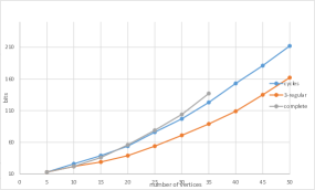
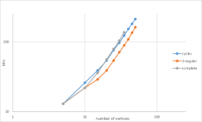
Figure 2: Number of bits required for the LLL step to recover the cycle space with probability $0.9$ vs. number of vertices. Log-Log on right.

For a fixed number of vertices (and hence edges), we used our implementation to search for the number of bits necessary for the probability (over random point sets) of the LLL step correctly identifying the cycle space of the graph to be at least $0.9$. (Here the configurations were integer, and the lengths were measured with $\{-1,0,1\}$ error.) For the nearly $3$-regular graphs, we tried $5$ different random ensembles and used the maximum number of bits required for each size. These experiments are “optimistic”, since they use knowledge of the number of vertices to avoid using a threshold value to identify small vectors in the reduced lattice basis.

In these results, we see that for all $3$ families of graphs, the bit requirement grows at about the rate $n^{1.5}$ (see the log-log plot of Figure 2). More bits are needed for the cycle graphs than the nearly $3$-regular graphs. This is perhaps due to the fact that the nearly $3$-regular graphs have basis cycles, with each cycle much smaller than $n$. For the complete graphs, where $m=O(n^{2})$, this gives us growth that is somewhat sub-linear in $m$. All of this behaviour is significantly better than the pessimistic $m^{2}$ bounds of our theory. On the other hand, even for moderate sized graphs, the required bit accuracy quickly becomes higher than we would be able to get from a physical measurement system.

References

- Bixby and Cunningham [1980] R. E. Bixby and W. H. Cunningham. Converting linear programs to network problems. Math. Oper. Res., 5(3):321–357, 1980. doi: 10.1287/moor.5.3.321.
- Cieliebak et al. [2003] M. Cieliebak, S. Eidenbenz, and P. Penna. Noisy data make the partial digest problem np-hard. In International Workshop on Algorithms in Bioinformatics, pages 111–123. Springer, 2003.
- Connelly [2005] R. Connelly. Generic global rigidity. Discrete Comput. Geom., 33(4):549–563, 2005. doi: 10.1007/s00454-004-1124-4.
- Frieze [1986] A. M. Frieze. On the Lagarias-Odlyzko algorithm for the subset sum problem. SIAM J. Comput., 15(2):536–539, 1986. doi: 10.1137/0215038.
- Gamarnik et al. [2019] D. Gamarnik, E. C. Kızıldağ, and I. Zadik. Inference in high-dimensional linear regression via lattice basis reduction and integer relation detection. arXiv preprint arXiv:1910.10890, 2019.
- Gkioulekas et al. [2017] I. Gkioulekas, S. J. Gortler, L. Theran, and T. Zickler. Determining generic point configurations from unlabeled path or loop lengths. Preprint, 2017. arXiv: 1709.03936.
- Gortler et al. [2010] S. J. Gortler, A. D. Healy, and D. P. Thurston. Characterizing generic global rigidity. Amer. J. Math., 132(4):897–939, 2010. doi: 10.1353/ajm.0.0132.
- Gortler et al. [2019] S. J. Gortler, L. Theran, and D. P. Thurston. Generic unlabeled global rigidity. In Forum of Mathematics, Sigma, volume 7. Cambridge University Press, 2019.
- Juhás et al. [2006] P. Juhás, D. Cherba, P. Duxbury, W. Punch, and S. Billinge. Ab initio determination of solid-state nanostructure. Nature, 440(7084):655–658, 2006.
- Lagarias and Odlyzko [1985] J. C. Lagarias and A. M. Odlyzko. Solving low-density subset sum problems. J. Assoc. Comput. Mach., 32(1):229–246, 1985. doi: 10.1145/2455.2461.
- Lemke et al. [2003] P. Lemke, S. S. Skiena, and W. D. Smith. Reconstructing sets from interpoint distances. In Discrete and computational geometry, pages 597–631. Springer, 2003.
- Lenstra et al. [1982] A. K. Lenstra, H. W. Lenstra, Jr., and L. Lovász. Factoring polynomials with rational coefficients. Math. Ann., 261(4):515–534, 1982. doi: 10.1007/BF01457454.
- Nguyen and Stehlé [2006] P. Q. Nguyen and D. Stehlé. LLL on the average. In International Algorithmic Number Theory Symposium, pages 238–256. Springer, 2006.
- Oxley [2011] J. Oxley. Matroid theory, volume 21 of Oxford Graduate Texts in Mathematics. Oxford University Press, Oxford, second edition, 2011. ISBN 978-0-19-960339-8. doi: 10.1093/acprof:oso/9780198566946.001.0001.
- Saxe [1979] J. B. Saxe. Embeddability of weighted graphs in -space is strongly NP-hard. In Proceedings of the 17th Allerton Conference in Communications, Control and Computing, pages 480–489, 1979.
- Seymour [1981] P. D. Seymour. Recognizing graphic matroids. Combinatorica, 1(1):75–78, 1981. doi: 10.1007/BF02579179.
- Skiena and Sundaram [1994] S. S. Skiena and G. Sundaram. A partial digest approach to restriction site mapping. Bulletin of Mathematical Biology, 56(2):275–294, 1994.
- So and Ye [2006] A. M.-C. So and Y. Ye. A semidefinite programming approach to tensegrity theory and realizability of graphs. In Proceedings of the seventeenth annual ACM-SIAM symposium on Discrete algorithm, pages 766–775. Society for Industrial and Applied Mathematics, 2006.
- Tutte [1960] W. T. Tutte. An algorithm for determining whether a given binary matroid is graphic. Proc. Amer. Math. Soc., 11:905–917, 1960. doi: 10.2307/2034435.
- Whitney [1933] H. Whitney. 2-Isomorphic Graphs. Amer. J. Math., 55(1-4):245–254, 1933. doi: 10.2307/2371127.
- Whitney [1935] H. Whitney. On the Abstract Properties of Linear Dependence. Amer. J. Math., 57(3):509–533, 1935. doi: 10.2307/2371182.
- Zadik and Gamarnik [2018] I. Zadik and D. Gamarnik. High dimensional linear regression using lattice basis reduction. In Advances in Neural Information Processing Systems 31, pages 1842–1852. 2018.