PRI-VAE: Principle-of-Relevant-Information Variational Autoencoders

Yanjun Li, Shujian Yu1, Jose C. Principe, Xiaolin Li, and Dapeng Wu1 Yanjun Li, Jose C. Principe and Dapeng Wu are with the NSF Center for Big Learning, University of Florida, U.S.A (email: yanjun.li@ufl.edu, principe@cnel.ufl.edu and dpwu@ufl.edu)Shujian Yu is with the Machine Learning Group, NEC Laboratories Europe, Germany (email: Shujian.Yu@neclab.eu).Xiaolin Li is with the Cognization Lab (email: xiaolinli@ieee.org).1 To whom correspondence should be addressed.
Abstract

Although substantial efforts have been made to learn disentangled representations under the variational autoencoder (VAE) framework, the fundamental properties to the dynamics of learning of most VAE models still remain unknown and under-investigated. In this work, we first propose a novel learning objective, termed the principle-of-relevant-information variational autoencoder (PRI-VAE), to learn disentangled representations. We then present an information-theoretic perspective to analyze existing VAE models by inspecting the evolution of some critical information-theoretic quantities across training epochs. Our observations unveil some fundamental properties associated with VAEs. Empirical results also demonstrate the effectiveness of PRI-VAE on four benchmark data sets.

Index Terms:
Disentangled representation learning, variational autoencoder, principle of relevant information.

I Introduction

A central goal for representation learning models is that the resulting latent representation should be compact yet disentangled. Compact requires the representation 𝐳𝐳\mathbf{z} does not contain any nuance factors in the input signal 𝐱𝐱\mathbf{x} that are not relevant for the desired response 𝐲𝐲\mathbf{y} [1], whereas disentangled means that 𝐳𝐳\mathbf{z} is factorizable and has consistent semantics associated to different generating factors of the underlying data generation process. To achieve this goal in an unsupervised fashion, different variational autoencoder (VAE) [12] based models have been developed in recent years by formulating the objective as finding an informative latent representation that can minimize reconstruction error under proper regularizations. Well-known regularizations include the channel capacity [5] and the total correlation [31] associated with each dimension of 𝐳𝐳\mathbf{z} [11, 7].

Despite these recent efforts, the fundamental properties of the dynamics of learning for most existing VAE models still remain unknown and under-investigated. Information theory provides a solid methodology to analyze the dynamics of learning and different trade-offs in deep neural networks (DNNs) [28]. This is because the encoding, the decoding, and the compression are precisely among the core problems information theory was made to solve. Therefore, a natural idea is to analyze existing VAE models by inspecting the evolution of some key information-theoretic quantities associated with the latent representations across training epochs. Albeit easy-to-understand, estimating information-theoretic quantities (such as mutual information) exactly in high-dimensional space is problematic [20]. As a result, current attempts (e.g., [2, 1]) on interpreting VAE models still lie on using rate-distortion (RD) theory [8, Chapter 10] to approximately compare the RD trade-off of different VAEs or illuminating its connection to the famed Information Bottleneck (IB) [29].

In this work, we address aforementioned problems by deriving a novel VAE objective from a first principle. We also suggest a novel estimator to evaluate mutual information and total correlation in VAEs; and illuminate its usage on analyzing and interpreting VAEs. Our contributions are fourfold:

  • We propose a novel VAE objective based on the principle of relevant information [22, Chapter 8]. We term it PRI-VAE and establish its connections to other VAEs.

  • We introduce the recently developed matrix-based Rényi’s α𝛼\alpha-entropy functional estimator [27, 34] to measure the mutual information 𝐈(𝐱;𝐳)𝐈𝐱𝐳\mathbf{I}(\mathbf{x};\mathbf{z}) and the total correlation 𝐓(𝐳)𝐓𝐳\mathbf{T}(\mathbf{z}) of different VAEs across training epochs.

  • We observed that, with the common stochastic gradient descent (SGD) optimization, both 𝐈(𝐱;𝐳)𝐈𝐱𝐳\mathbf{I}(\mathbf{x};\mathbf{z}) and 𝐓(𝐳)𝐓𝐳\mathbf{T}(\mathbf{z}) increase rapidly at the first few epochs and then continuously decrease in the remaining epochs. We also observed a positive correlation between 𝐈(𝐱;𝐳)𝐈𝐱𝐳\mathbf{I}(\mathbf{x};\mathbf{z}) and 𝐓(𝐳)𝐓𝐳\mathbf{T}(\mathbf{z}).

  • Experiments on the four benchmark data sets suggest that PRI-VAE encourages more disentangled representations and reasonable reconstruction quality with fewer training epochs. We also demonstrate the flexibility of PRI-VAE and generalize its idea to a higher level.

II Preliminary Knowledge

II-A VAE and the Evidence Lower Bound

A VAE operates with two probabilistic mappings, an encoder XZmaps-to𝑋𝑍X\mapsto Z (represented by a neural network with parameter ϕitalic-ϕ\phi), and a decoder (ZXmaps-to𝑍𝑋Z\mapsto X represented by another neural network with parameter θ𝜃\theta). Normally, we assume a fixed prior distribution p(𝐳)𝑝𝐳p(\mathbf{z}) over 𝐳𝐳\mathbf{z}. Since the distribution of 𝐱𝐱\mathbf{x} is also fixed (i.e., the data distribution q(𝐱)𝑞𝐱q(\mathbf{x})), the encoder and decoder induce joint distributions q(𝐱,𝐳)=qϕ(𝐳|𝐱)q(𝐱)𝑞𝐱𝐳subscript𝑞italic-ϕconditional𝐳𝐱𝑞𝐱q(\mathbf{x},\mathbf{z})=q_{\phi}(\mathbf{z}|\mathbf{x})q(\mathbf{x}) and p(𝐱,𝐳)=pθ(𝐱|𝐳)p(𝐳)𝑝𝐱𝐳subscript𝑝𝜃conditional𝐱𝐳𝑝𝐳p(\mathbf{x},\mathbf{z})=p_{\theta}(\mathbf{x}|\mathbf{z})p(\mathbf{z}), respectively. An ideal VAE objective is to maximize the marginalized log-likelihood:

𝔼p(𝐱)[logpθ(𝐱)].subscript𝔼𝑝𝐱delimited-[]subscript𝑝𝜃𝐱\mathbb{E}_{p(\mathbf{x})}[\log p_{\theta}(\mathbf{x})].\\ (1)

Eq. (1) is, however, not tractable and is approximated by the evidence lower bound (ELBO) [12]:

𝔼q(𝐳|𝐱)[logp(𝐱|𝐳)]𝔼p(𝐱)[DKL(qϕ(𝐳|𝐱)p(𝐳))],subscript𝔼𝑞conditional𝐳𝐱delimited-[]𝑝conditional𝐱𝐳subscript𝔼𝑝𝐱delimited-[]subscript𝐷𝐾𝐿conditionalsubscript𝑞italic-ϕconditional𝐳𝐱𝑝𝐳\mathbb{E}_{q(\mathbf{z}|\mathbf{x})}[\log p(\mathbf{x}|\mathbf{z})]-\mathbb{E}_{p(\mathbf{x})}[D_{KL}(q_{\phi}(\mathbf{z}|\mathbf{x})\|p(\mathbf{z}))],\\ (2)

where the first term measures the reconstruction loss, and the second one is the regularization term, which corresponds to the Kullback-Leibler (KL) divergence between the latent distribution qϕ(𝐳|𝐱)subscript𝑞italic-ϕconditional𝐳𝐱q_{\phi}(\mathbf{z}|\mathbf{x}) and the prior distribution p(𝐳)𝑝𝐳p(\mathbf{z}). Usually, we assume p(𝐳)𝑝𝐳p(\mathbf{z}) follows a standard isotropic multivariate normal distribution 𝒩(0,I)𝒩0𝐼\mathcal{N}(0,I) where I𝐼I is the identify matrix.

II-B PRI: the General Idea and its Objective

PRI is an unsupervised information-theoretic principle that aims to perform mode decomposition of a random variable X𝑋X with a known (and fixed) probability distribution g𝑔g. Suppose we obtain a reduced statistical representation characterized by a random variable Y𝑌Y with probability distribution f𝑓f.

The PRI casts this problem as a trade-off between the entropy 𝐇(f)𝐇𝑓\mathbf{H}(f) of Y𝑌Y and its descriptive power about X𝑋X in terms of their divergence D(fg)𝐷conditional𝑓𝑔D(f\|g):

J(f)=argminf𝐇(f)+γD(fg),𝐽𝑓subscriptargmin𝑓𝐇𝑓𝛾𝐷conditional𝑓𝑔J(f)=\operatorname*{arg\,min}\limits_{f}\mathbf{H}(f)+\gamma D(f\|g), (3)

where γ𝛾\gamma is a hyper-parameter controlling the amount of relevant information that Y𝑌Y can extract from X𝑋X. The minimization of entropy can be viewed as a means of reducing uncertainty (or redundancy) and finding the statistical regularities in the outcomes of a process, whereas the minimization of information divergence ensures that such regularities are closely related to X𝑋X. The PRI is similar in spirit to the IB approach, but the formulation is different because PRI does not require a relevant auxiliary variable Z𝑍Z and the optimization is done directly on the random variable X𝑋X.

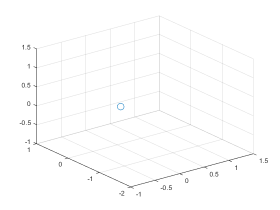
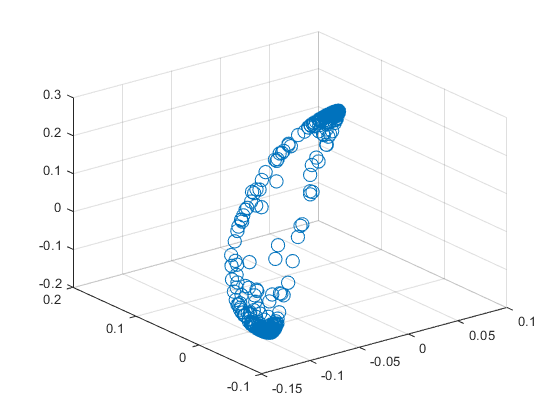
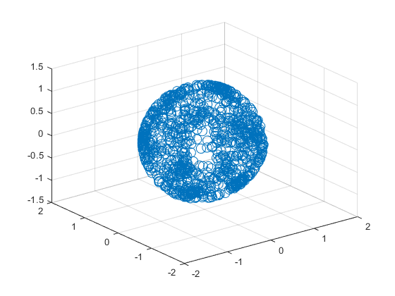
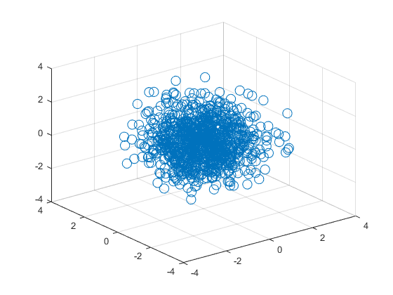
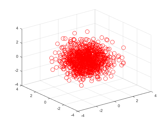
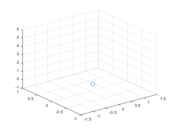
Note that the choice of entropy and divergence is application-specific and depends mostly on the simplicity of optimization. Although this work still uses the basic Shannon’s differential entropy and the KL divergence for a fair comparison, the 222-order Rényi’s entropy functional [25] and the Parzen window density estimator [21] evidence a long track record of usefulness in various machine learning applications [22]. Fig. 1 illustrates a set of solutions revealed by PRI that are related to the principal curves or surfaces.
Refer to caption
(a) 3d Gaussian.
Refer to caption
(b) γ=0𝛾0\gamma=0
Refer to caption
(c) γ=1𝛾1\gamma=1
Refer to caption
(d) γ=2𝛾2\gamma=2
Refer to caption
(e) γ=5𝛾5\gamma=5
Refer to caption
(f) γ=100𝛾100\gamma=100
Figure 1: Illustration of the structures revealed by the PRI for (a) a 3d isotropic Gaussian. As the values of γ𝛾\gamma increase, the solution passes through (b) a single point, (c) mode, (d) principal curves, (e) principal surfaces, and in the extreme case of (f) γ𝛾\gamma\rightarrow\infty we get back the data themselves as the solution.

III PRI-VAE

As mentioned earlier, a good latent representation 𝐳𝐳\mathbf{z} should be compact yet disentangled. We thus propose the following VAE objective:

PRIVAE=𝔼p(𝐱)[𝔼q(𝐳|𝐱)[logp(𝐱|𝐳)]α𝐇(𝐳)βDKL[qϕ(𝐳)p(𝐳)].\begin{split}\mathcal{L}_{\mathrm{PRI-VAE}}&=\mathbb{E}_{p(\mathbf{x})}\left[\mathbb{E}_{q(\mathbf{z}|\mathbf{x})}\left[\log p(\mathbf{x}|\mathbf{z})\right]\right.\\ &-\alpha\mathbf{H}(\mathbf{z})-\beta D_{KL}[q_{\phi}(\mathbf{z})\|p(\mathbf{z})].\\[3.0pt] \end{split} (4)

Eq. (4) has three terms, but each term has its own physical meaning. 𝔼p(𝐱)[𝔼q(𝐳|𝐱)[logp(𝐱|𝐳)]\mathbb{E}_{p(\mathbf{x})}\left[\mathbb{E}_{q(\mathbf{z}|\mathbf{x})}\left[\log p(\mathbf{x}|\mathbf{z})\right]\right. guarantees a reliable reconstruction of input 𝐱𝐱\mathbf{x} from latent representation 𝐳𝐳\mathbf{z}. α𝐇(𝐳)𝛼𝐇𝐳\alpha\mathbf{H}(\mathbf{z}) regularizes the uncertainty or the degree of compactness in 𝐳𝐳\mathbf{z}: a large α𝛼\alpha encourages our model to learn a more compact latent representation, whereas a small α𝛼\alpha may lead to the latent representation contains nuisance factors that are irrelevant for downstream tasks. On the other hand, β𝛽\beta controls the closeness between qϕ(𝐳)subscript𝑞italic-ϕ𝐳q_{\phi}(\mathbf{z}) and p(𝐳)𝑝𝐳p(\mathbf{z}), which can be interpreted as the extent of disentanglement of 𝐳𝐳\mathbf{z}: a large β𝛽\beta enforces the independence in each dimension of 𝐳𝐳\mathbf{z}, and should, therefore, be preferred. One should note that, the combination of α𝐇(𝐳)+βDKL[qϕ(𝐳)p(𝐳)]𝛼𝐇𝐳𝛽subscript𝐷𝐾𝐿delimited-[]conditionalsubscript𝑞italic-ϕ𝐳𝑝𝐳\alpha\mathbf{H}(\mathbf{z})+\beta D_{KL}[q_{\phi}(\mathbf{z})\|p(\mathbf{z})] is exactly the objective of PRI, in which the ratio β/α𝛽𝛼\beta/\alpha plays the same role as γ𝛾\gamma in Eq. (3). We therefore term Eq. (4) the principle-of-relevant-information variational autoencoder (PRI-VAE).

III-A Optimizing the PRI-VAE

To optimize the PRI-VAE objective, we need to compute the inference marginal q(𝐳)=𝔼p(𝐱)[q(𝐳|𝐱)]𝑞𝐳subscript𝔼𝑝𝐱delimited-[]𝑞conditional𝐳𝐱q(\mathbf{z})=\mathbb{E}_{p(\mathbf{x})}[q(\mathbf{z}|\mathbf{x})]. However, in practice, exactly computing its value is intractable in the training phase, since it depends on the entire data set. In PRI-VAE, we use the weighted Monte Carlo approximation suggested in [7] to estimate q(𝐳)𝑞𝐳q(\mathbf{z}), as it does not require additional hyper-parameters or inner optimization loops.

III-B Relation to Prior Art

In this section, we establish the connections between PRI-VAE and other recently developed VAEs.

β𝛽\beta-VAE [10] learns disentangled representation by introducing a hyper-parameter β𝛽\beta (usually β>1𝛽1\beta>1) to heavily penalize the term DKL(qϕ(𝐳|𝐱)p(𝐳))subscript𝐷𝐾𝐿conditionalsubscript𝑞italic-ϕconditional𝐳𝐱𝑝𝐳D_{KL}(q_{\phi}(\mathbf{z}|\mathbf{x})\|p(\mathbf{z})) in Eq. (2). The emergence of disentanglement can be simply explained if we decompose 𝔼p(𝐱)[DKL(qϕ(𝐳|𝐱)p(𝐳))]subscript𝔼𝑝𝐱delimited-[]subscript𝐷𝐾𝐿conditionalsubscript𝑞italic-ϕconditional𝐳𝐱𝑝𝐳\mathbb{E}_{p(\mathbf{x})}[D_{KL}(q_{\phi}(\mathbf{z}|\mathbf{x})\|p(\mathbf{z}))] as (see proof in [11]):

𝐈(𝐱;𝐳)1+DKL(qϕ(𝐳)p(𝐳)2).\underbrace{\mathbf{I}(\mathbf{x};\mathbf{z})}_{\leavevmode\hbox to7.29pt{\vbox to7.29pt{\pgfpicture\makeatletter\hbox{\hskip 3.64555pt\lower-3.64555pt\hbox to0.0pt{\pgfsys@beginscope\pgfsys@invoke{ }\definecolor{pgfstrokecolor}{rgb}{0,0,0}\pgfsys@color@rgb@stroke{0}{0}{0}\pgfsys@invoke{ }\pgfsys@color@rgb@fill{0}{0}{0}\pgfsys@invoke{ }\pgfsys@setlinewidth{0.4pt}\pgfsys@invoke{ }\nullfont\hbox to0.0pt{\pgfsys@beginscope\pgfsys@invoke{ }{{{}}\hbox{\hbox{{\pgfsys@beginscope\pgfsys@invoke{ }{{}{{{}}}{{}}{}{}{}{}{}{}{}{}{}{{}\pgfsys@moveto{3.44556pt}{0.0pt}\pgfsys@curveto{3.44556pt}{1.90294pt}{1.90294pt}{3.44556pt}{0.0pt}{3.44556pt}\pgfsys@curveto{-1.90294pt}{3.44556pt}{-3.44556pt}{1.90294pt}{-3.44556pt}{0.0pt}\pgfsys@curveto{-3.44556pt}{-1.90294pt}{-1.90294pt}{-3.44556pt}{0.0pt}{-3.44556pt}\pgfsys@curveto{1.90294pt}{-3.44556pt}{3.44556pt}{-1.90294pt}{3.44556pt}{0.0pt}\pgfsys@closepath\pgfsys@moveto{0.0pt}{0.0pt}\pgfsys@stroke\pgfsys@invoke{ } }{{{{}}\pgfsys@beginscope\pgfsys@invoke{ }\pgfsys@transformcm{1.0}{0.0}{0.0}{1.0}{-1.25pt}{-1.6111pt}\pgfsys@invoke{ }\hbox{{\definecolor{pgfstrokecolor}{rgb}{0,0,0}\pgfsys@color@rgb@stroke{0}{0}{0}\pgfsys@invoke{ }\pgfsys@color@rgb@fill{0}{0}{0}\pgfsys@invoke{ }\hbox{{\tiny 1}} }}\pgfsys@invoke{\lxSVG@closescope }\pgfsys@endscope}}} \pgfsys@invoke{\lxSVG@closescope }\pgfsys@endscope}}} } \pgfsys@invoke{\lxSVG@closescope }\pgfsys@endscope{{{}}}{}{}\hss}\pgfsys@discardpath\pgfsys@invoke{\lxSVG@closescope }\pgfsys@endscope\hss}}\lxSVG@closescope\endpgfpicture}}}+\underbrace{D_{KL}(q_{\phi}(\mathbf{z})\|p(\mathbf{z})}_{\leavevmode\hbox to7.29pt{\vbox to7.29pt{\pgfpicture\makeatletter\hbox{\hskip 3.64555pt\lower-3.64555pt\hbox to0.0pt{\pgfsys@beginscope\pgfsys@invoke{ }\definecolor{pgfstrokecolor}{rgb}{0,0,0}\pgfsys@color@rgb@stroke{0}{0}{0}\pgfsys@invoke{ }\pgfsys@color@rgb@fill{0}{0}{0}\pgfsys@invoke{ }\pgfsys@setlinewidth{0.4pt}\pgfsys@invoke{ }\nullfont\hbox to0.0pt{\pgfsys@beginscope\pgfsys@invoke{ }{{{}}\hbox{\hbox{{\pgfsys@beginscope\pgfsys@invoke{ }{{}{{{}}}{{}}{}{}{}{}{}{}{}{}{}{{}\pgfsys@moveto{3.44556pt}{0.0pt}\pgfsys@curveto{3.44556pt}{1.90294pt}{1.90294pt}{3.44556pt}{0.0pt}{3.44556pt}\pgfsys@curveto{-1.90294pt}{3.44556pt}{-3.44556pt}{1.90294pt}{-3.44556pt}{0.0pt}\pgfsys@curveto{-3.44556pt}{-1.90294pt}{-1.90294pt}{-3.44556pt}{0.0pt}{-3.44556pt}\pgfsys@curveto{1.90294pt}{-3.44556pt}{3.44556pt}{-1.90294pt}{3.44556pt}{0.0pt}\pgfsys@closepath\pgfsys@moveto{0.0pt}{0.0pt}\pgfsys@stroke\pgfsys@invoke{ } }{{{{}}\pgfsys@beginscope\pgfsys@invoke{ }\pgfsys@transformcm{1.0}{0.0}{0.0}{1.0}{-1.25pt}{-1.6111pt}\pgfsys@invoke{ }\hbox{{\definecolor{pgfstrokecolor}{rgb}{0,0,0}\pgfsys@color@rgb@stroke{0}{0}{0}\pgfsys@invoke{ }\pgfsys@color@rgb@fill{0}{0}{0}\pgfsys@invoke{ }\hbox{{\tiny 2}} }}\pgfsys@invoke{\lxSVG@closescope }\pgfsys@endscope}}} \pgfsys@invoke{\lxSVG@closescope }\pgfsys@endscope}}} } \pgfsys@invoke{\lxSVG@closescope }\pgfsys@endscope{{{}}}{}{}\hss}\pgfsys@discardpath\pgfsys@invoke{\lxSVG@closescope }\pgfsys@endscope\hss}}\lxSVG@closescope\endpgfpicture}}}).\\ (5)

To address this limitation, DIP-VAE [14] and InfoVAE [36] suggest assigning different weights to the two terms in Eq. (5). Moreover, suppose p(𝐳)𝑝𝐳p(\mathbf{z}) is factorizable, 2 can be further decomposed as [11, 7]:

2=DKL(q(𝐳)j=1q(𝐳j)A+dDKL(qϕ(𝐳j)p(𝐳j))B),\begin{split}&\leavevmode\hbox to9.75pt{\vbox to9.75pt{\pgfpicture\makeatletter\hbox{\hskip 4.87285pt\lower-4.87285pt\hbox to0.0pt{\pgfsys@beginscope\pgfsys@invoke{ }\definecolor{pgfstrokecolor}{rgb}{0,0,0}\pgfsys@color@rgb@stroke{0}{0}{0}\pgfsys@invoke{ }\pgfsys@color@rgb@fill{0}{0}{0}\pgfsys@invoke{ }\pgfsys@setlinewidth{0.4pt}\pgfsys@invoke{ }\nullfont\hbox to0.0pt{\pgfsys@beginscope\pgfsys@invoke{ }{{{}}\hbox{\hbox{{\pgfsys@beginscope\pgfsys@invoke{ }{{}{{{}}}{{}}{}{}{}{}{}{}{}{}{}{{}\pgfsys@moveto{4.67285pt}{0.0pt}\pgfsys@curveto{4.67285pt}{2.58076pt}{2.58076pt}{4.67285pt}{0.0pt}{4.67285pt}\pgfsys@curveto{-2.58076pt}{4.67285pt}{-4.67285pt}{2.58076pt}{-4.67285pt}{0.0pt}\pgfsys@curveto{-4.67285pt}{-2.58076pt}{-2.58076pt}{-4.67285pt}{0.0pt}{-4.67285pt}\pgfsys@curveto{2.58076pt}{-4.67285pt}{4.67285pt}{-2.58076pt}{4.67285pt}{0.0pt}\pgfsys@closepath\pgfsys@moveto{0.0pt}{0.0pt}\pgfsys@stroke\pgfsys@invoke{ } }{{{{}}\pgfsys@beginscope\pgfsys@invoke{ }\pgfsys@transformcm{1.0}{0.0}{0.0}{1.0}{-2.0pt}{-2.57777pt}\pgfsys@invoke{ }\hbox{{\definecolor{pgfstrokecolor}{rgb}{0,0,0}\pgfsys@color@rgb@stroke{0}{0}{0}\pgfsys@invoke{ }\pgfsys@color@rgb@fill{0}{0}{0}\pgfsys@invoke{ }\hbox{{\footnotesize 2}} }}\pgfsys@invoke{\lxSVG@closescope }\pgfsys@endscope}}} \pgfsys@invoke{\lxSVG@closescope }\pgfsys@endscope}}} } \pgfsys@invoke{\lxSVG@closescope }\pgfsys@endscope{{{}}}{}{}\hss}\pgfsys@discardpath\pgfsys@invoke{\lxSVG@closescope }\pgfsys@endscope\hss}}\lxSVG@closescope\endpgfpicture}}=\underbrace{D_{KL}(q(\mathbf{z})\|\prod\limits_{j=1}q(\mathbf{z}_{j})}_{\leavevmode\hbox to8.27pt{\vbox to8.27pt{\pgfpicture\makeatletter\hbox{\hskip 4.13579pt\lower-4.13579pt\hbox to0.0pt{\pgfsys@beginscope\pgfsys@invoke{ }\definecolor{pgfstrokecolor}{rgb}{0,0,0}\pgfsys@color@rgb@stroke{0}{0}{0}\pgfsys@invoke{ }\pgfsys@color@rgb@fill{0}{0}{0}\pgfsys@invoke{ }\pgfsys@setlinewidth{0.4pt}\pgfsys@invoke{ }\nullfont\hbox to0.0pt{\pgfsys@beginscope\pgfsys@invoke{ }{{{}}\hbox{\hbox{{\pgfsys@beginscope\pgfsys@invoke{ }{{}{{{}}}{{}}{}{}{}{}{}{}{}{}{}{{}\pgfsys@moveto{3.93579pt}{0.0pt}\pgfsys@curveto{3.93579pt}{2.17369pt}{2.17369pt}{3.93579pt}{0.0pt}{3.93579pt}\pgfsys@curveto{-2.17369pt}{3.93579pt}{-3.93579pt}{2.17369pt}{-3.93579pt}{0.0pt}\pgfsys@curveto{-3.93579pt}{-2.17369pt}{-2.17369pt}{-3.93579pt}{0.0pt}{-3.93579pt}\pgfsys@curveto{2.17369pt}{-3.93579pt}{3.93579pt}{-2.17369pt}{3.93579pt}{0.0pt}\pgfsys@closepath\pgfsys@moveto{0.0pt}{0.0pt}\pgfsys@stroke\pgfsys@invoke{ } }{{{{}}\pgfsys@beginscope\pgfsys@invoke{ }\pgfsys@transformcm{1.0}{0.0}{0.0}{1.0}{-1.875pt}{-1.70833pt}\pgfsys@invoke{ }\hbox{{\definecolor{pgfstrokecolor}{rgb}{0,0,0}\pgfsys@color@rgb@stroke{0}{0}{0}\pgfsys@invoke{ }\pgfsys@color@rgb@fill{0}{0}{0}\pgfsys@invoke{ }\hbox{{\tiny A}} }}\pgfsys@invoke{\lxSVG@closescope }\pgfsys@endscope}}} \pgfsys@invoke{\lxSVG@closescope }\pgfsys@endscope}}} } \pgfsys@invoke{\lxSVG@closescope }\pgfsys@endscope{{{}}}{}{}\hss}\pgfsys@discardpath\pgfsys@invoke{\lxSVG@closescope }\pgfsys@endscope\hss}}\lxSVG@closescope\endpgfpicture}}}+\sum_{d}\underbrace{\operatorname{D_{KL}}\left(q_{\phi}\left(\mathbf{z}_{j}\right)\|p\left(\mathbf{z}_{j}\right)\right)}_{\leavevmode\hbox to8.15pt{\vbox to8.15pt{\pgfpicture\makeatletter\hbox{\hskip 4.07597pt\lower-4.07597pt\hbox to0.0pt{\pgfsys@beginscope\pgfsys@invoke{ }\definecolor{pgfstrokecolor}{rgb}{0,0,0}\pgfsys@color@rgb@stroke{0}{0}{0}\pgfsys@invoke{ }\pgfsys@color@rgb@fill{0}{0}{0}\pgfsys@invoke{ }\pgfsys@setlinewidth{0.4pt}\pgfsys@invoke{ }\nullfont\hbox to0.0pt{\pgfsys@beginscope\pgfsys@invoke{ }{{{}}\hbox{\hbox{{\pgfsys@beginscope\pgfsys@invoke{ }{{}{{{}}}{{}}{}{}{}{}{}{}{}{}{}{{}\pgfsys@moveto{3.87598pt}{0.0pt}\pgfsys@curveto{3.87598pt}{2.14066pt}{2.14066pt}{3.87598pt}{0.0pt}{3.87598pt}\pgfsys@curveto{-2.14066pt}{3.87598pt}{-3.87598pt}{2.14066pt}{-3.87598pt}{0.0pt}\pgfsys@curveto{-3.87598pt}{-2.14066pt}{-2.14066pt}{-3.87598pt}{0.0pt}{-3.87598pt}\pgfsys@curveto{2.14066pt}{-3.87598pt}{3.87598pt}{-2.14066pt}{3.87598pt}{0.0pt}\pgfsys@closepath\pgfsys@moveto{0.0pt}{0.0pt}\pgfsys@stroke\pgfsys@invoke{ } }{{{{}}\pgfsys@beginscope\pgfsys@invoke{ }\pgfsys@transformcm{1.0}{0.0}{0.0}{1.0}{-1.77083pt}{-1.70833pt}\pgfsys@invoke{ }\hbox{{\definecolor{pgfstrokecolor}{rgb}{0,0,0}\pgfsys@color@rgb@stroke{0}{0}{0}\pgfsys@invoke{ }\pgfsys@color@rgb@fill{0}{0}{0}\pgfsys@invoke{ }\hbox{{\tiny B}} }}\pgfsys@invoke{\lxSVG@closescope }\pgfsys@endscope}}} \pgfsys@invoke{\lxSVG@closescope }\pgfsys@endscope}}} } \pgfsys@invoke{\lxSVG@closescope }\pgfsys@endscope{{{}}}{}{}\hss}\pgfsys@discardpath\pgfsys@invoke{\lxSVG@closescope }\pgfsys@endscope\hss}}\lxSVG@closescope\endpgfpicture}}}),\\[3.0pt] \end{split} (6)

where term A is the total correlation regularization associated with each dimension of 𝐳𝐳\mathbf{z} and term B refers to the dimension-wise KL divergence (d𝑑d is the dimension of 𝐳𝐳\mathbf{z}), which controls the penalty on the deviation between each latent dimension to the prior. FactorVAE [11] and β𝛽\beta-TCVAE [7] add an external penalty on A to encourage the independence in each dimension of 𝐳𝐳\mathbf{z}.

Before our work, IB approach (e.g., [1]) suggests a restriction on 𝐈(𝐱;𝐳)𝐈𝐱𝐳\mathbf{I}(\mathbf{x};\mathbf{z}) in Eq. (5) to keep 𝐳𝐳\mathbf{z} from containing nuance factors, whereas [2, 5] introduce a hard constraint on the channel capacity to make sure 𝐈(𝐱;𝐳)𝐈𝐱𝐳\mathbf{I}(\mathbf{x};\mathbf{z}) is consistently larger than a predefined value. PRI-VAE absorbs both proposals by flexibly adjusting the value of β/α𝛽𝛼\beta/\alpha: a large α𝛼\alpha penalizes more on 𝐇(𝐳)𝐇𝐳\mathbf{H}(\mathbf{z}) (and hence 𝐈(𝐱;𝐳)𝐈𝐱𝐳\mathbf{I}(\mathbf{x};\mathbf{z}), because 𝐈(𝐱;𝐳)𝐈𝐱𝐳\mathbf{I}(\mathbf{x};\mathbf{z}) is always saturated [9]) in practice, whereas a small α𝛼\alpha avoids 𝐇(𝐳)𝐇𝐳\mathbf{H}(\mathbf{z}) reducing to zero, which also prevents a small channel capacity 𝐈(𝐱;𝐳)𝐈𝐱𝐳\mathbf{I}(\mathbf{x};\mathbf{z}). In an extreme case, when α=0𝛼0\alpha=0, we get back to the InfoVAE objective. We provide, in Table I, an overview of objectives in different VAE models.

TABLE I: Objectives of different VAE models. 1superscript1\leavevmode\hbox to9.75pt{\vbox to9.75pt{\pgfpicture\makeatletter\hbox{\hskip 4.87285pt\lower-4.87285pt\hbox to0.0pt{\pgfsys@beginscope\pgfsys@invoke{ }\definecolor{pgfstrokecolor}{rgb}{0,0,0}\pgfsys@color@rgb@stroke{0}{0}{0}\pgfsys@invoke{ }\pgfsys@color@rgb@fill{0}{0}{0}\pgfsys@invoke{ }\pgfsys@setlinewidth{0.4pt}\pgfsys@invoke{ }\nullfont\hbox to0.0pt{\pgfsys@beginscope\pgfsys@invoke{ }{{{}}\hbox{\hbox{{\pgfsys@beginscope\pgfsys@invoke{ }{{}{{{}}}{{}}{}{}{}{}{}{}{}{}{}{{}\pgfsys@moveto{4.67285pt}{0.0pt}\pgfsys@curveto{4.67285pt}{2.58076pt}{2.58076pt}{4.67285pt}{0.0pt}{4.67285pt}\pgfsys@curveto{-2.58076pt}{4.67285pt}{-4.67285pt}{2.58076pt}{-4.67285pt}{0.0pt}\pgfsys@curveto{-4.67285pt}{-2.58076pt}{-2.58076pt}{-4.67285pt}{0.0pt}{-4.67285pt}\pgfsys@curveto{2.58076pt}{-4.67285pt}{4.67285pt}{-2.58076pt}{4.67285pt}{0.0pt}\pgfsys@closepath\pgfsys@moveto{0.0pt}{0.0pt}\pgfsys@stroke\pgfsys@invoke{ } }{{{{}}\pgfsys@beginscope\pgfsys@invoke{ }\pgfsys@transformcm{1.0}{0.0}{0.0}{1.0}{-2.0pt}{-2.57777pt}\pgfsys@invoke{ }\hbox{{\definecolor{pgfstrokecolor}{rgb}{0,0,0}\pgfsys@color@rgb@stroke{0}{0}{0}\pgfsys@invoke{ }\pgfsys@color@rgb@fill{0}{0}{0}\pgfsys@invoke{ }\hbox{{\footnotesize 1}} }}\pgfsys@invoke{\lxSVG@closescope }\pgfsys@endscope}}} \pgfsys@invoke{\lxSVG@closescope }\pgfsys@endscope}}} } \pgfsys@invoke{\lxSVG@closescope }\pgfsys@endscope{{{}}}{}{}\hss}\pgfsys@discardpath\pgfsys@invoke{\lxSVG@closescope }\pgfsys@endscope\hss}}\lxSVG@closescope\endpgfpicture}}^{*} represents the 𝐇(𝐳)𝐇𝐳\mathbf{H}(\mathbf{z}) term, which is a tight upper bound of the term 1.
Method Reconstruction term Regularization term
β𝛽\beta-VAE [10] 𝔼q(𝐳|𝐱)[logp(𝐱|𝐳)]subscript𝔼𝑞conditional𝐳𝐱delimited-[]𝑝conditional𝐱𝐳\mathbb{E}_{q(\mathbf{z}|\mathbf{x})}[\log p(\mathbf{x}|\mathbf{z})] β(1+2)𝛽12\beta(\leavevmode\hbox to9.75pt{\vbox to9.75pt{\pgfpicture\makeatletter\hbox{\hskip 4.87285pt\lower-4.87285pt\hbox to0.0pt{\pgfsys@beginscope\pgfsys@invoke{ }\definecolor{pgfstrokecolor}{rgb}{0,0,0}\pgfsys@color@rgb@stroke{0}{0}{0}\pgfsys@invoke{ }\pgfsys@color@rgb@fill{0}{0}{0}\pgfsys@invoke{ }\pgfsys@setlinewidth{0.4pt}\pgfsys@invoke{ }\nullfont\hbox to0.0pt{\pgfsys@beginscope\pgfsys@invoke{ }{{{}}\hbox{\hbox{{\pgfsys@beginscope\pgfsys@invoke{ }{{}{{{}}}{{}}{}{}{}{}{}{}{}{}{}{{}\pgfsys@moveto{4.67285pt}{0.0pt}\pgfsys@curveto{4.67285pt}{2.58076pt}{2.58076pt}{4.67285pt}{0.0pt}{4.67285pt}\pgfsys@curveto{-2.58076pt}{4.67285pt}{-4.67285pt}{2.58076pt}{-4.67285pt}{0.0pt}\pgfsys@curveto{-4.67285pt}{-2.58076pt}{-2.58076pt}{-4.67285pt}{0.0pt}{-4.67285pt}\pgfsys@curveto{2.58076pt}{-4.67285pt}{4.67285pt}{-2.58076pt}{4.67285pt}{0.0pt}\pgfsys@closepath\pgfsys@moveto{0.0pt}{0.0pt}\pgfsys@stroke\pgfsys@invoke{ } }{{{{}}\pgfsys@beginscope\pgfsys@invoke{ }\pgfsys@transformcm{1.0}{0.0}{0.0}{1.0}{-2.0pt}{-2.57777pt}\pgfsys@invoke{ }\hbox{{\definecolor{pgfstrokecolor}{rgb}{0,0,0}\pgfsys@color@rgb@stroke{0}{0}{0}\pgfsys@invoke{ }\pgfsys@color@rgb@fill{0}{0}{0}\pgfsys@invoke{ }\hbox{{\footnotesize 1}} }}\pgfsys@invoke{\lxSVG@closescope }\pgfsys@endscope}}} \pgfsys@invoke{\lxSVG@closescope }\pgfsys@endscope}}} } \pgfsys@invoke{\lxSVG@closescope }\pgfsys@endscope{{{}}}{}{}\hss}\pgfsys@discardpath\pgfsys@invoke{\lxSVG@closescope }\pgfsys@endscope\hss}}\lxSVG@closescope\endpgfpicture}}+\leavevmode\hbox to9.75pt{\vbox to9.75pt{\pgfpicture\makeatletter\hbox{\hskip 4.87285pt\lower-4.87285pt\hbox to0.0pt{\pgfsys@beginscope\pgfsys@invoke{ }\definecolor{pgfstrokecolor}{rgb}{0,0,0}\pgfsys@color@rgb@stroke{0}{0}{0}\pgfsys@invoke{ }\pgfsys@color@rgb@fill{0}{0}{0}\pgfsys@invoke{ }\pgfsys@setlinewidth{0.4pt}\pgfsys@invoke{ }\nullfont\hbox to0.0pt{\pgfsys@beginscope\pgfsys@invoke{ }{{{}}\hbox{\hbox{{\pgfsys@beginscope\pgfsys@invoke{ }{{}{{{}}}{{}}{}{}{}{}{}{}{}{}{}{{}\pgfsys@moveto{4.67285pt}{0.0pt}\pgfsys@curveto{4.67285pt}{2.58076pt}{2.58076pt}{4.67285pt}{0.0pt}{4.67285pt}\pgfsys@curveto{-2.58076pt}{4.67285pt}{-4.67285pt}{2.58076pt}{-4.67285pt}{0.0pt}\pgfsys@curveto{-4.67285pt}{-2.58076pt}{-2.58076pt}{-4.67285pt}{0.0pt}{-4.67285pt}\pgfsys@curveto{2.58076pt}{-4.67285pt}{4.67285pt}{-2.58076pt}{4.67285pt}{0.0pt}\pgfsys@closepath\pgfsys@moveto{0.0pt}{0.0pt}\pgfsys@stroke\pgfsys@invoke{ } }{{{{}}\pgfsys@beginscope\pgfsys@invoke{ }\pgfsys@transformcm{1.0}{0.0}{0.0}{1.0}{-2.0pt}{-2.57777pt}\pgfsys@invoke{ }\hbox{{\definecolor{pgfstrokecolor}{rgb}{0,0,0}\pgfsys@color@rgb@stroke{0}{0}{0}\pgfsys@invoke{ }\pgfsys@color@rgb@fill{0}{0}{0}\pgfsys@invoke{ }\hbox{{\footnotesize 2}} }}\pgfsys@invoke{\lxSVG@closescope }\pgfsys@endscope}}} \pgfsys@invoke{\lxSVG@closescope }\pgfsys@endscope}}} } \pgfsys@invoke{\lxSVG@closescope }\pgfsys@endscope{{{}}}{}{}\hss}\pgfsys@discardpath\pgfsys@invoke{\lxSVG@closescope }\pgfsys@endscope\hss}}\lxSVG@closescope\endpgfpicture}})
AnnealedVAE [5] γ|(1+2)C|𝛾12𝐶\gamma|(\leavevmode\hbox to9.75pt{\vbox to9.75pt{\pgfpicture\makeatletter\hbox{\hskip 4.87285pt\lower-4.87285pt\hbox to0.0pt{\pgfsys@beginscope\pgfsys@invoke{ }\definecolor{pgfstrokecolor}{rgb}{0,0,0}\pgfsys@color@rgb@stroke{0}{0}{0}\pgfsys@invoke{ }\pgfsys@color@rgb@fill{0}{0}{0}\pgfsys@invoke{ }\pgfsys@setlinewidth{0.4pt}\pgfsys@invoke{ }\nullfont\hbox to0.0pt{\pgfsys@beginscope\pgfsys@invoke{ }{{{}}\hbox{\hbox{{\pgfsys@beginscope\pgfsys@invoke{ }{{}{{{}}}{{}}{}{}{}{}{}{}{}{}{}{{}\pgfsys@moveto{4.67285pt}{0.0pt}\pgfsys@curveto{4.67285pt}{2.58076pt}{2.58076pt}{4.67285pt}{0.0pt}{4.67285pt}\pgfsys@curveto{-2.58076pt}{4.67285pt}{-4.67285pt}{2.58076pt}{-4.67285pt}{0.0pt}\pgfsys@curveto{-4.67285pt}{-2.58076pt}{-2.58076pt}{-4.67285pt}{0.0pt}{-4.67285pt}\pgfsys@curveto{2.58076pt}{-4.67285pt}{4.67285pt}{-2.58076pt}{4.67285pt}{0.0pt}\pgfsys@closepath\pgfsys@moveto{0.0pt}{0.0pt}\pgfsys@stroke\pgfsys@invoke{ } }{{{{}}\pgfsys@beginscope\pgfsys@invoke{ }\pgfsys@transformcm{1.0}{0.0}{0.0}{1.0}{-2.0pt}{-2.57777pt}\pgfsys@invoke{ }\hbox{{\definecolor{pgfstrokecolor}{rgb}{0,0,0}\pgfsys@color@rgb@stroke{0}{0}{0}\pgfsys@invoke{ }\pgfsys@color@rgb@fill{0}{0}{0}\pgfsys@invoke{ }\hbox{{\footnotesize 1}} }}\pgfsys@invoke{\lxSVG@closescope }\pgfsys@endscope}}} \pgfsys@invoke{\lxSVG@closescope }\pgfsys@endscope}}} } \pgfsys@invoke{\lxSVG@closescope }\pgfsys@endscope{{{}}}{}{}\hss}\pgfsys@discardpath\pgfsys@invoke{\lxSVG@closescope }\pgfsys@endscope\hss}}\lxSVG@closescope\endpgfpicture}}+\leavevmode\hbox to9.75pt{\vbox to9.75pt{\pgfpicture\makeatletter\hbox{\hskip 4.87285pt\lower-4.87285pt\hbox to0.0pt{\pgfsys@beginscope\pgfsys@invoke{ }\definecolor{pgfstrokecolor}{rgb}{0,0,0}\pgfsys@color@rgb@stroke{0}{0}{0}\pgfsys@invoke{ }\pgfsys@color@rgb@fill{0}{0}{0}\pgfsys@invoke{ }\pgfsys@setlinewidth{0.4pt}\pgfsys@invoke{ }\nullfont\hbox to0.0pt{\pgfsys@beginscope\pgfsys@invoke{ }{{{}}\hbox{\hbox{{\pgfsys@beginscope\pgfsys@invoke{ }{{}{{{}}}{{}}{}{}{}{}{}{}{}{}{}{{}\pgfsys@moveto{4.67285pt}{0.0pt}\pgfsys@curveto{4.67285pt}{2.58076pt}{2.58076pt}{4.67285pt}{0.0pt}{4.67285pt}\pgfsys@curveto{-2.58076pt}{4.67285pt}{-4.67285pt}{2.58076pt}{-4.67285pt}{0.0pt}\pgfsys@curveto{-4.67285pt}{-2.58076pt}{-2.58076pt}{-4.67285pt}{0.0pt}{-4.67285pt}\pgfsys@curveto{2.58076pt}{-4.67285pt}{4.67285pt}{-2.58076pt}{4.67285pt}{0.0pt}\pgfsys@closepath\pgfsys@moveto{0.0pt}{0.0pt}\pgfsys@stroke\pgfsys@invoke{ } }{{{{}}\pgfsys@beginscope\pgfsys@invoke{ }\pgfsys@transformcm{1.0}{0.0}{0.0}{1.0}{-2.0pt}{-2.57777pt}\pgfsys@invoke{ }\hbox{{\definecolor{pgfstrokecolor}{rgb}{0,0,0}\pgfsys@color@rgb@stroke{0}{0}{0}\pgfsys@invoke{ }\pgfsys@color@rgb@fill{0}{0}{0}\pgfsys@invoke{ }\hbox{{\footnotesize 2}} }}\pgfsys@invoke{\lxSVG@closescope }\pgfsys@endscope}}} \pgfsys@invoke{\lxSVG@closescope }\pgfsys@endscope}}} } \pgfsys@invoke{\lxSVG@closescope }\pgfsys@endscope{{{}}}{}{}\hss}\pgfsys@discardpath\pgfsys@invoke{\lxSVG@closescope }\pgfsys@endscope\hss}}\lxSVG@closescope\endpgfpicture}})-C|
DIP-VAE [14] 1+λ21𝜆2\leavevmode\hbox to9.75pt{\vbox to9.75pt{\pgfpicture\makeatletter\hbox{\hskip 4.87285pt\lower-4.87285pt\hbox to0.0pt{\pgfsys@beginscope\pgfsys@invoke{ }\definecolor{pgfstrokecolor}{rgb}{0,0,0}\pgfsys@color@rgb@stroke{0}{0}{0}\pgfsys@invoke{ }\pgfsys@color@rgb@fill{0}{0}{0}\pgfsys@invoke{ }\pgfsys@setlinewidth{0.4pt}\pgfsys@invoke{ }\nullfont\hbox to0.0pt{\pgfsys@beginscope\pgfsys@invoke{ }{{{}}\hbox{\hbox{{\pgfsys@beginscope\pgfsys@invoke{ }{{}{{{}}}{{}}{}{}{}{}{}{}{}{}{}{{}\pgfsys@moveto{4.67285pt}{0.0pt}\pgfsys@curveto{4.67285pt}{2.58076pt}{2.58076pt}{4.67285pt}{0.0pt}{4.67285pt}\pgfsys@curveto{-2.58076pt}{4.67285pt}{-4.67285pt}{2.58076pt}{-4.67285pt}{0.0pt}\pgfsys@curveto{-4.67285pt}{-2.58076pt}{-2.58076pt}{-4.67285pt}{0.0pt}{-4.67285pt}\pgfsys@curveto{2.58076pt}{-4.67285pt}{4.67285pt}{-2.58076pt}{4.67285pt}{0.0pt}\pgfsys@closepath\pgfsys@moveto{0.0pt}{0.0pt}\pgfsys@stroke\pgfsys@invoke{ } }{{{{}}\pgfsys@beginscope\pgfsys@invoke{ }\pgfsys@transformcm{1.0}{0.0}{0.0}{1.0}{-2.0pt}{-2.57777pt}\pgfsys@invoke{ }\hbox{{\definecolor{pgfstrokecolor}{rgb}{0,0,0}\pgfsys@color@rgb@stroke{0}{0}{0}\pgfsys@invoke{ }\pgfsys@color@rgb@fill{0}{0}{0}\pgfsys@invoke{ }\hbox{{\footnotesize 1}} }}\pgfsys@invoke{\lxSVG@closescope }\pgfsys@endscope}}} \pgfsys@invoke{\lxSVG@closescope }\pgfsys@endscope}}} } \pgfsys@invoke{\lxSVG@closescope }\pgfsys@endscope{{{}}}{}{}\hss}\pgfsys@discardpath\pgfsys@invoke{\lxSVG@closescope }\pgfsys@endscope\hss}}\lxSVG@closescope\endpgfpicture}}+\lambda\leavevmode\hbox to9.75pt{\vbox to9.75pt{\pgfpicture\makeatletter\hbox{\hskip 4.87285pt\lower-4.87285pt\hbox to0.0pt{\pgfsys@beginscope\pgfsys@invoke{ }\definecolor{pgfstrokecolor}{rgb}{0,0,0}\pgfsys@color@rgb@stroke{0}{0}{0}\pgfsys@invoke{ }\pgfsys@color@rgb@fill{0}{0}{0}\pgfsys@invoke{ }\pgfsys@setlinewidth{0.4pt}\pgfsys@invoke{ }\nullfont\hbox to0.0pt{\pgfsys@beginscope\pgfsys@invoke{ }{{{}}\hbox{\hbox{{\pgfsys@beginscope\pgfsys@invoke{ }{{}{{{}}}{{}}{}{}{}{}{}{}{}{}{}{{}\pgfsys@moveto{4.67285pt}{0.0pt}\pgfsys@curveto{4.67285pt}{2.58076pt}{2.58076pt}{4.67285pt}{0.0pt}{4.67285pt}\pgfsys@curveto{-2.58076pt}{4.67285pt}{-4.67285pt}{2.58076pt}{-4.67285pt}{0.0pt}\pgfsys@curveto{-4.67285pt}{-2.58076pt}{-2.58076pt}{-4.67285pt}{0.0pt}{-4.67285pt}\pgfsys@curveto{2.58076pt}{-4.67285pt}{4.67285pt}{-2.58076pt}{4.67285pt}{0.0pt}\pgfsys@closepath\pgfsys@moveto{0.0pt}{0.0pt}\pgfsys@stroke\pgfsys@invoke{ } }{{{{}}\pgfsys@beginscope\pgfsys@invoke{ }\pgfsys@transformcm{1.0}{0.0}{0.0}{1.0}{-2.0pt}{-2.57777pt}\pgfsys@invoke{ }\hbox{{\definecolor{pgfstrokecolor}{rgb}{0,0,0}\pgfsys@color@rgb@stroke{0}{0}{0}\pgfsys@invoke{ }\pgfsys@color@rgb@fill{0}{0}{0}\pgfsys@invoke{ }\hbox{{\footnotesize 2}} }}\pgfsys@invoke{\lxSVG@closescope }\pgfsys@endscope}}} \pgfsys@invoke{\lxSVG@closescope }\pgfsys@endscope}}} } \pgfsys@invoke{\lxSVG@closescope }\pgfsys@endscope{{{}}}{}{}\hss}\pgfsys@discardpath\pgfsys@invoke{\lxSVG@closescope }\pgfsys@endscope\hss}}\lxSVG@closescope\endpgfpicture}}
InfoVAE [36] λ2𝜆2\lambda\leavevmode\hbox to9.75pt{\vbox to9.75pt{\pgfpicture\makeatletter\hbox{\hskip 4.87285pt\lower-4.87285pt\hbox to0.0pt{\pgfsys@beginscope\pgfsys@invoke{ }\definecolor{pgfstrokecolor}{rgb}{0,0,0}\pgfsys@color@rgb@stroke{0}{0}{0}\pgfsys@invoke{ }\pgfsys@color@rgb@fill{0}{0}{0}\pgfsys@invoke{ }\pgfsys@setlinewidth{0.4pt}\pgfsys@invoke{ }\nullfont\hbox to0.0pt{\pgfsys@beginscope\pgfsys@invoke{ }{{{}}\hbox{\hbox{{\pgfsys@beginscope\pgfsys@invoke{ }{{}{{{}}}{{}}{}{}{}{}{}{}{}{}{}{{}\pgfsys@moveto{4.67285pt}{0.0pt}\pgfsys@curveto{4.67285pt}{2.58076pt}{2.58076pt}{4.67285pt}{0.0pt}{4.67285pt}\pgfsys@curveto{-2.58076pt}{4.67285pt}{-4.67285pt}{2.58076pt}{-4.67285pt}{0.0pt}\pgfsys@curveto{-4.67285pt}{-2.58076pt}{-2.58076pt}{-4.67285pt}{0.0pt}{-4.67285pt}\pgfsys@curveto{2.58076pt}{-4.67285pt}{4.67285pt}{-2.58076pt}{4.67285pt}{0.0pt}\pgfsys@closepath\pgfsys@moveto{0.0pt}{0.0pt}\pgfsys@stroke\pgfsys@invoke{ } }{{{{}}\pgfsys@beginscope\pgfsys@invoke{ }\pgfsys@transformcm{1.0}{0.0}{0.0}{1.0}{-2.0pt}{-2.57777pt}\pgfsys@invoke{ }\hbox{{\definecolor{pgfstrokecolor}{rgb}{0,0,0}\pgfsys@color@rgb@stroke{0}{0}{0}\pgfsys@invoke{ }\pgfsys@color@rgb@fill{0}{0}{0}\pgfsys@invoke{ }\hbox{{\footnotesize 2}} }}\pgfsys@invoke{\lxSVG@closescope }\pgfsys@endscope}}} \pgfsys@invoke{\lxSVG@closescope }\pgfsys@endscope}}} } \pgfsys@invoke{\lxSVG@closescope }\pgfsys@endscope{{{}}}{}{}\hss}\pgfsys@discardpath\pgfsys@invoke{\lxSVG@closescope }\pgfsys@endscope\hss}}\lxSVG@closescope\endpgfpicture}}
FactorVAE [11] 1+γA+B1𝛾AB\leavevmode\hbox to9.75pt{\vbox to9.75pt{\pgfpicture\makeatletter\hbox{\hskip 4.87285pt\lower-4.87285pt\hbox to0.0pt{\pgfsys@beginscope\pgfsys@invoke{ }\definecolor{pgfstrokecolor}{rgb}{0,0,0}\pgfsys@color@rgb@stroke{0}{0}{0}\pgfsys@invoke{ }\pgfsys@color@rgb@fill{0}{0}{0}\pgfsys@invoke{ }\pgfsys@setlinewidth{0.4pt}\pgfsys@invoke{ }\nullfont\hbox to0.0pt{\pgfsys@beginscope\pgfsys@invoke{ }{{{}}\hbox{\hbox{{\pgfsys@beginscope\pgfsys@invoke{ }{{}{{{}}}{{}}{}{}{}{}{}{}{}{}{}{{}\pgfsys@moveto{4.67285pt}{0.0pt}\pgfsys@curveto{4.67285pt}{2.58076pt}{2.58076pt}{4.67285pt}{0.0pt}{4.67285pt}\pgfsys@curveto{-2.58076pt}{4.67285pt}{-4.67285pt}{2.58076pt}{-4.67285pt}{0.0pt}\pgfsys@curveto{-4.67285pt}{-2.58076pt}{-2.58076pt}{-4.67285pt}{0.0pt}{-4.67285pt}\pgfsys@curveto{2.58076pt}{-4.67285pt}{4.67285pt}{-2.58076pt}{4.67285pt}{0.0pt}\pgfsys@closepath\pgfsys@moveto{0.0pt}{0.0pt}\pgfsys@stroke\pgfsys@invoke{ } }{{{{}}\pgfsys@beginscope\pgfsys@invoke{ }\pgfsys@transformcm{1.0}{0.0}{0.0}{1.0}{-2.0pt}{-2.57777pt}\pgfsys@invoke{ }\hbox{{\definecolor{pgfstrokecolor}{rgb}{0,0,0}\pgfsys@color@rgb@stroke{0}{0}{0}\pgfsys@invoke{ }\pgfsys@color@rgb@fill{0}{0}{0}\pgfsys@invoke{ }\hbox{{\footnotesize 1}} }}\pgfsys@invoke{\lxSVG@closescope }\pgfsys@endscope}}} \pgfsys@invoke{\lxSVG@closescope }\pgfsys@endscope}}} } \pgfsys@invoke{\lxSVG@closescope }\pgfsys@endscope{{{}}}{}{}\hss}\pgfsys@discardpath\pgfsys@invoke{\lxSVG@closescope }\pgfsys@endscope\hss}}\lxSVG@closescope\endpgfpicture}}+\gamma\leavevmode\hbox to11.35pt{\vbox to11.35pt{\pgfpicture\makeatletter\hbox{\hskip 5.67583pt\lower-5.67583pt\hbox to0.0pt{\pgfsys@beginscope\pgfsys@invoke{ }\definecolor{pgfstrokecolor}{rgb}{0,0,0}\pgfsys@color@rgb@stroke{0}{0}{0}\pgfsys@invoke{ }\pgfsys@color@rgb@fill{0}{0}{0}\pgfsys@invoke{ }\pgfsys@setlinewidth{0.4pt}\pgfsys@invoke{ }\nullfont\hbox to0.0pt{\pgfsys@beginscope\pgfsys@invoke{ }{{{}}\hbox{\hbox{{\pgfsys@beginscope\pgfsys@invoke{ }{{}{{{}}}{{}}{}{}{}{}{}{}{}{}{}{{}\pgfsys@moveto{5.47583pt}{0.0pt}\pgfsys@curveto{5.47583pt}{3.02425pt}{3.02425pt}{5.47583pt}{0.0pt}{5.47583pt}\pgfsys@curveto{-3.02425pt}{5.47583pt}{-5.47583pt}{3.02425pt}{-5.47583pt}{0.0pt}\pgfsys@curveto{-5.47583pt}{-3.02425pt}{-3.02425pt}{-5.47583pt}{0.0pt}{-5.47583pt}\pgfsys@curveto{3.02425pt}{-5.47583pt}{5.47583pt}{-3.02425pt}{5.47583pt}{0.0pt}\pgfsys@closepath\pgfsys@moveto{0.0pt}{0.0pt}\pgfsys@stroke\pgfsys@invoke{ } }{{{{}}\pgfsys@beginscope\pgfsys@invoke{ }\pgfsys@transformcm{1.0}{0.0}{0.0}{1.0}{-3.0pt}{-2.73332pt}\pgfsys@invoke{ }\hbox{{\definecolor{pgfstrokecolor}{rgb}{0,0,0}\pgfsys@color@rgb@stroke{0}{0}{0}\pgfsys@invoke{ }\pgfsys@color@rgb@fill{0}{0}{0}\pgfsys@invoke{ }\hbox{{\footnotesize A}} }}\pgfsys@invoke{\lxSVG@closescope }\pgfsys@endscope}}} \pgfsys@invoke{\lxSVG@closescope }\pgfsys@endscope}}} } \pgfsys@invoke{\lxSVG@closescope }\pgfsys@endscope{{{}}}{}{}\hss}\pgfsys@discardpath\pgfsys@invoke{\lxSVG@closescope }\pgfsys@endscope\hss}}\lxSVG@closescope\endpgfpicture}}+\leavevmode\hbox to11.07pt{\vbox to11.07pt{\pgfpicture\makeatletter\hbox{\hskip 5.53325pt\lower-5.53325pt\hbox to0.0pt{\pgfsys@beginscope\pgfsys@invoke{ }\definecolor{pgfstrokecolor}{rgb}{0,0,0}\pgfsys@color@rgb@stroke{0}{0}{0}\pgfsys@invoke{ }\pgfsys@color@rgb@fill{0}{0}{0}\pgfsys@invoke{ }\pgfsys@setlinewidth{0.4pt}\pgfsys@invoke{ }\nullfont\hbox to0.0pt{\pgfsys@beginscope\pgfsys@invoke{ }{{{}}\hbox{\hbox{{\pgfsys@beginscope\pgfsys@invoke{ }{{}{{{}}}{{}}{}{}{}{}{}{}{}{}{}{{}\pgfsys@moveto{5.33325pt}{0.0pt}\pgfsys@curveto{5.33325pt}{2.94551pt}{2.94551pt}{5.33325pt}{0.0pt}{5.33325pt}\pgfsys@curveto{-2.94551pt}{5.33325pt}{-5.33325pt}{2.94551pt}{-5.33325pt}{0.0pt}\pgfsys@curveto{-5.33325pt}{-2.94551pt}{-2.94551pt}{-5.33325pt}{0.0pt}{-5.33325pt}\pgfsys@curveto{2.94551pt}{-5.33325pt}{5.33325pt}{-2.94551pt}{5.33325pt}{0.0pt}\pgfsys@closepath\pgfsys@moveto{0.0pt}{0.0pt}\pgfsys@stroke\pgfsys@invoke{ } }{{{{}}\pgfsys@beginscope\pgfsys@invoke{ }\pgfsys@transformcm{1.0}{0.0}{0.0}{1.0}{-2.83334pt}{-2.73332pt}\pgfsys@invoke{ }\hbox{{\definecolor{pgfstrokecolor}{rgb}{0,0,0}\pgfsys@color@rgb@stroke{0}{0}{0}\pgfsys@invoke{ }\pgfsys@color@rgb@fill{0}{0}{0}\pgfsys@invoke{ }\hbox{{\footnotesize B}} }}\pgfsys@invoke{\lxSVG@closescope }\pgfsys@endscope}}} \pgfsys@invoke{\lxSVG@closescope }\pgfsys@endscope}}} } \pgfsys@invoke{\lxSVG@closescope }\pgfsys@endscope{{{}}}{}{}\hss}\pgfsys@discardpath\pgfsys@invoke{\lxSVG@closescope }\pgfsys@endscope\hss}}\lxSVG@closescope\endpgfpicture}}
β𝛽\beta-TCVAE [7] 1+βA+B1𝛽AB\leavevmode\hbox to9.75pt{\vbox to9.75pt{\pgfpicture\makeatletter\hbox{\hskip 4.87285pt\lower-4.87285pt\hbox to0.0pt{\pgfsys@beginscope\pgfsys@invoke{ }\definecolor{pgfstrokecolor}{rgb}{0,0,0}\pgfsys@color@rgb@stroke{0}{0}{0}\pgfsys@invoke{ }\pgfsys@color@rgb@fill{0}{0}{0}\pgfsys@invoke{ }\pgfsys@setlinewidth{0.4pt}\pgfsys@invoke{ }\nullfont\hbox to0.0pt{\pgfsys@beginscope\pgfsys@invoke{ }{{{}}\hbox{\hbox{{\pgfsys@beginscope\pgfsys@invoke{ }{{}{{{}}}{{}}{}{}{}{}{}{}{}{}{}{{}\pgfsys@moveto{4.67285pt}{0.0pt}\pgfsys@curveto{4.67285pt}{2.58076pt}{2.58076pt}{4.67285pt}{0.0pt}{4.67285pt}\pgfsys@curveto{-2.58076pt}{4.67285pt}{-4.67285pt}{2.58076pt}{-4.67285pt}{0.0pt}\pgfsys@curveto{-4.67285pt}{-2.58076pt}{-2.58076pt}{-4.67285pt}{0.0pt}{-4.67285pt}\pgfsys@curveto{2.58076pt}{-4.67285pt}{4.67285pt}{-2.58076pt}{4.67285pt}{0.0pt}\pgfsys@closepath\pgfsys@moveto{0.0pt}{0.0pt}\pgfsys@stroke\pgfsys@invoke{ } }{{{{}}\pgfsys@beginscope\pgfsys@invoke{ }\pgfsys@transformcm{1.0}{0.0}{0.0}{1.0}{-2.0pt}{-2.57777pt}\pgfsys@invoke{ }\hbox{{\definecolor{pgfstrokecolor}{rgb}{0,0,0}\pgfsys@color@rgb@stroke{0}{0}{0}\pgfsys@invoke{ }\pgfsys@color@rgb@fill{0}{0}{0}\pgfsys@invoke{ }\hbox{{\footnotesize 1}} }}\pgfsys@invoke{\lxSVG@closescope }\pgfsys@endscope}}} \pgfsys@invoke{\lxSVG@closescope }\pgfsys@endscope}}} } \pgfsys@invoke{\lxSVG@closescope }\pgfsys@endscope{{{}}}{}{}\hss}\pgfsys@discardpath\pgfsys@invoke{\lxSVG@closescope }\pgfsys@endscope\hss}}\lxSVG@closescope\endpgfpicture}}+\beta\leavevmode\hbox to11.35pt{\vbox to11.35pt{\pgfpicture\makeatletter\hbox{\hskip 5.67583pt\lower-5.67583pt\hbox to0.0pt{\pgfsys@beginscope\pgfsys@invoke{ }\definecolor{pgfstrokecolor}{rgb}{0,0,0}\pgfsys@color@rgb@stroke{0}{0}{0}\pgfsys@invoke{ }\pgfsys@color@rgb@fill{0}{0}{0}\pgfsys@invoke{ }\pgfsys@setlinewidth{0.4pt}\pgfsys@invoke{ }\nullfont\hbox to0.0pt{\pgfsys@beginscope\pgfsys@invoke{ }{{{}}\hbox{\hbox{{\pgfsys@beginscope\pgfsys@invoke{ }{{}{{{}}}{{}}{}{}{}{}{}{}{}{}{}{{}\pgfsys@moveto{5.47583pt}{0.0pt}\pgfsys@curveto{5.47583pt}{3.02425pt}{3.02425pt}{5.47583pt}{0.0pt}{5.47583pt}\pgfsys@curveto{-3.02425pt}{5.47583pt}{-5.47583pt}{3.02425pt}{-5.47583pt}{0.0pt}\pgfsys@curveto{-5.47583pt}{-3.02425pt}{-3.02425pt}{-5.47583pt}{0.0pt}{-5.47583pt}\pgfsys@curveto{3.02425pt}{-5.47583pt}{5.47583pt}{-3.02425pt}{5.47583pt}{0.0pt}\pgfsys@closepath\pgfsys@moveto{0.0pt}{0.0pt}\pgfsys@stroke\pgfsys@invoke{ } }{{{{}}\pgfsys@beginscope\pgfsys@invoke{ }\pgfsys@transformcm{1.0}{0.0}{0.0}{1.0}{-3.0pt}{-2.73332pt}\pgfsys@invoke{ }\hbox{{\definecolor{pgfstrokecolor}{rgb}{0,0,0}\pgfsys@color@rgb@stroke{0}{0}{0}\pgfsys@invoke{ }\pgfsys@color@rgb@fill{0}{0}{0}\pgfsys@invoke{ }\hbox{{\footnotesize A}} }}\pgfsys@invoke{\lxSVG@closescope }\pgfsys@endscope}}} \pgfsys@invoke{\lxSVG@closescope }\pgfsys@endscope}}} } \pgfsys@invoke{\lxSVG@closescope }\pgfsys@endscope{{{}}}{}{}\hss}\pgfsys@discardpath\pgfsys@invoke{\lxSVG@closescope }\pgfsys@endscope\hss}}\lxSVG@closescope\endpgfpicture}}+\leavevmode\hbox to11.07pt{\vbox to11.07pt{\pgfpicture\makeatletter\hbox{\hskip 5.53325pt\lower-5.53325pt\hbox to0.0pt{\pgfsys@beginscope\pgfsys@invoke{ }\definecolor{pgfstrokecolor}{rgb}{0,0,0}\pgfsys@color@rgb@stroke{0}{0}{0}\pgfsys@invoke{ }\pgfsys@color@rgb@fill{0}{0}{0}\pgfsys@invoke{ }\pgfsys@setlinewidth{0.4pt}\pgfsys@invoke{ }\nullfont\hbox to0.0pt{\pgfsys@beginscope\pgfsys@invoke{ }{{{}}\hbox{\hbox{{\pgfsys@beginscope\pgfsys@invoke{ }{{}{{{}}}{{}}{}{}{}{}{}{}{}{}{}{{}\pgfsys@moveto{5.33325pt}{0.0pt}\pgfsys@curveto{5.33325pt}{2.94551pt}{2.94551pt}{5.33325pt}{0.0pt}{5.33325pt}\pgfsys@curveto{-2.94551pt}{5.33325pt}{-5.33325pt}{2.94551pt}{-5.33325pt}{0.0pt}\pgfsys@curveto{-5.33325pt}{-2.94551pt}{-2.94551pt}{-5.33325pt}{0.0pt}{-5.33325pt}\pgfsys@curveto{2.94551pt}{-5.33325pt}{5.33325pt}{-2.94551pt}{5.33325pt}{0.0pt}\pgfsys@closepath\pgfsys@moveto{0.0pt}{0.0pt}\pgfsys@stroke\pgfsys@invoke{ } }{{{{}}\pgfsys@beginscope\pgfsys@invoke{ }\pgfsys@transformcm{1.0}{0.0}{0.0}{1.0}{-2.83334pt}{-2.73332pt}\pgfsys@invoke{ }\hbox{{\definecolor{pgfstrokecolor}{rgb}{0,0,0}\pgfsys@color@rgb@stroke{0}{0}{0}\pgfsys@invoke{ }\pgfsys@color@rgb@fill{0}{0}{0}\pgfsys@invoke{ }\hbox{{\footnotesize B}} }}\pgfsys@invoke{\lxSVG@closescope }\pgfsys@endscope}}} \pgfsys@invoke{\lxSVG@closescope }\pgfsys@endscope}}} } \pgfsys@invoke{\lxSVG@closescope }\pgfsys@endscope{{{}}}{}{}\hss}\pgfsys@discardpath\pgfsys@invoke{\lxSVG@closescope }\pgfsys@endscope\hss}}\lxSVG@closescope\endpgfpicture}}
PRI-VAE α1+β2𝛼superscript1𝛽2\alpha\leavevmode\hbox to9.75pt{\vbox to9.75pt{\pgfpicture\makeatletter\hbox{\hskip 4.87285pt\lower-4.87285pt\hbox to0.0pt{\pgfsys@beginscope\pgfsys@invoke{ }\definecolor{pgfstrokecolor}{rgb}{0,0,0}\pgfsys@color@rgb@stroke{0}{0}{0}\pgfsys@invoke{ }\pgfsys@color@rgb@fill{0}{0}{0}\pgfsys@invoke{ }\pgfsys@setlinewidth{0.4pt}\pgfsys@invoke{ }\nullfont\hbox to0.0pt{\pgfsys@beginscope\pgfsys@invoke{ }{{{}}\hbox{\hbox{{\pgfsys@beginscope\pgfsys@invoke{ }{{}{{{}}}{{}}{}{}{}{}{}{}{}{}{}{{}\pgfsys@moveto{4.67285pt}{0.0pt}\pgfsys@curveto{4.67285pt}{2.58076pt}{2.58076pt}{4.67285pt}{0.0pt}{4.67285pt}\pgfsys@curveto{-2.58076pt}{4.67285pt}{-4.67285pt}{2.58076pt}{-4.67285pt}{0.0pt}\pgfsys@curveto{-4.67285pt}{-2.58076pt}{-2.58076pt}{-4.67285pt}{0.0pt}{-4.67285pt}\pgfsys@curveto{2.58076pt}{-4.67285pt}{4.67285pt}{-2.58076pt}{4.67285pt}{0.0pt}\pgfsys@closepath\pgfsys@moveto{0.0pt}{0.0pt}\pgfsys@stroke\pgfsys@invoke{ } }{{{{}}\pgfsys@beginscope\pgfsys@invoke{ }\pgfsys@transformcm{1.0}{0.0}{0.0}{1.0}{-2.0pt}{-2.57777pt}\pgfsys@invoke{ }\hbox{{\definecolor{pgfstrokecolor}{rgb}{0,0,0}\pgfsys@color@rgb@stroke{0}{0}{0}\pgfsys@invoke{ }\pgfsys@color@rgb@fill{0}{0}{0}\pgfsys@invoke{ }\hbox{{\footnotesize 1}} }}\pgfsys@invoke{\lxSVG@closescope }\pgfsys@endscope}}} \pgfsys@invoke{\lxSVG@closescope }\pgfsys@endscope}}} } \pgfsys@invoke{\lxSVG@closescope }\pgfsys@endscope{{{}}}{}{}\hss}\pgfsys@discardpath\pgfsys@invoke{\lxSVG@closescope }\pgfsys@endscope\hss}}\lxSVG@closescope\endpgfpicture}}^{*}+\beta\leavevmode\hbox to9.75pt{\vbox to9.75pt{\pgfpicture\makeatletter\hbox{\hskip 4.87285pt\lower-4.87285pt\hbox to0.0pt{\pgfsys@beginscope\pgfsys@invoke{ }\definecolor{pgfstrokecolor}{rgb}{0,0,0}\pgfsys@color@rgb@stroke{0}{0}{0}\pgfsys@invoke{ }\pgfsys@color@rgb@fill{0}{0}{0}\pgfsys@invoke{ }\pgfsys@setlinewidth{0.4pt}\pgfsys@invoke{ }\nullfont\hbox to0.0pt{\pgfsys@beginscope\pgfsys@invoke{ }{{{}}\hbox{\hbox{{\pgfsys@beginscope\pgfsys@invoke{ }{{}{{{}}}{{}}{}{}{}{}{}{}{}{}{}{{}\pgfsys@moveto{4.67285pt}{0.0pt}\pgfsys@curveto{4.67285pt}{2.58076pt}{2.58076pt}{4.67285pt}{0.0pt}{4.67285pt}\pgfsys@curveto{-2.58076pt}{4.67285pt}{-4.67285pt}{2.58076pt}{-4.67285pt}{0.0pt}\pgfsys@curveto{-4.67285pt}{-2.58076pt}{-2.58076pt}{-4.67285pt}{0.0pt}{-4.67285pt}\pgfsys@curveto{2.58076pt}{-4.67285pt}{4.67285pt}{-2.58076pt}{4.67285pt}{0.0pt}\pgfsys@closepath\pgfsys@moveto{0.0pt}{0.0pt}\pgfsys@stroke\pgfsys@invoke{ } }{{{{}}\pgfsys@beginscope\pgfsys@invoke{ }\pgfsys@transformcm{1.0}{0.0}{0.0}{1.0}{-2.0pt}{-2.57777pt}\pgfsys@invoke{ }\hbox{{\definecolor{pgfstrokecolor}{rgb}{0,0,0}\pgfsys@color@rgb@stroke{0}{0}{0}\pgfsys@invoke{ }\pgfsys@color@rgb@fill{0}{0}{0}\pgfsys@invoke{ }\hbox{{\footnotesize 2}} }}\pgfsys@invoke{\lxSVG@closescope }\pgfsys@endscope}}} \pgfsys@invoke{\lxSVG@closescope }\pgfsys@endscope}}} } \pgfsys@invoke{\lxSVG@closescope }\pgfsys@endscope{{{}}}{}{}\hss}\pgfsys@discardpath\pgfsys@invoke{\lxSVG@closescope }\pgfsys@endscope\hss}}\lxSVG@closescope\endpgfpicture}}

IV Empirical behavior of 𝐈(𝐱;𝐳)𝐈𝐱𝐳\mathbf{I}(\mathbf{x};\mathbf{z}) and 𝐓(𝐳)𝐓𝐳\mathbf{T}(\mathbf{z})

Motivated by [28], we study disentanglement behavior and the learning dynamics of VAEs by measuring the evolution of 𝐈(𝐱;𝐳)𝐈𝐱𝐳\mathbf{I}(\mathbf{x};\mathbf{z}) and 𝐓(𝐳)𝐓𝐳\mathbf{T}(\mathbf{z}) across training epochs.

Given input 𝐱p𝐱superscript𝑝\mathbf{x}\in\mathbb{R}^{p} and latent representation 𝐳d𝐳superscript𝑑\mathbf{z}\in\mathbb{R}^{d}, the standard Shannon (differential) entropy functional defines 𝐈(𝐱;𝐳)𝐈𝐱𝐳\mathbf{I}(\mathbf{x};\mathbf{z}) and 𝐓(𝐳)𝐓𝐳\mathbf{T}(\mathbf{z}) with Eq. (7) and Eq. (8), respectively:

𝐈(𝐱;𝐳)=DKL(p(𝐱,𝐳)p(𝐱)p(𝐳))=p(𝐱,𝐳)log(p(𝐱,𝐳)p(𝐱)p(𝐳))𝑑𝐱𝑑𝐳𝐈𝐱𝐳subscript𝐷KLconditional𝑝𝐱𝐳𝑝𝐱𝑝𝐳𝑝𝐱𝐳𝑝𝐱𝐳𝑝𝐱𝑝𝐳differential-d𝐱differential-d𝐳\begin{split}\mathbf{I}(\mathbf{x};\mathbf{z})&=D_{\text{KL}}\left(p(\mathbf{x},\mathbf{z})\|p(\mathbf{x})p(\mathbf{z})\right)\\ &=\int\int p(\mathbf{x},\mathbf{z})\log\left(\frac{p(\mathbf{x},\mathbf{z})}{p(\mathbf{x})p(\mathbf{z})}\right)d\mathbf{x}d\mathbf{z}\end{split} (7)
𝐓(𝐳)=DKL(p(𝐳)p(z1)p(zd))=p(𝐳)log(p(𝐳)p(z1)p(zd))𝑑z1𝑑zd𝐓𝐳subscript𝐷KLconditional𝑝𝐳𝑝subscript𝑧1𝑝subscript𝑧𝑑𝑝𝐳𝑝𝐳𝑝subscript𝑧1𝑝subscript𝑧𝑑differential-dsubscript𝑧1differential-dsubscript𝑧𝑑\begin{split}\mathbf{T}(\mathbf{z})&=D_{\text{KL}}\left(p(\mathbf{z})\|p(z_{1})\cdots p(z_{d})\right)\\ &=\int\cdots\int p(\mathbf{z})\log\left(\frac{p(\mathbf{z})}{p(z_{1})\cdots p(z_{d})}\right)dz_{1}\cdots dz_{d}\end{split} (8)

As can be seen, a precise estimation to the joint distribution p(𝐱,𝐳)𝑝𝐱𝐳p(\mathbf{x},\mathbf{z}) or p(z1,z2,,zd)𝑝subscript𝑧1subscript𝑧2subscript𝑧𝑑p(z_{1},z_{2},\cdots,z_{d}) is a prerequisite to obtain a reliable evaluation to both 𝐈(𝐱;𝐳)𝐈𝐱𝐳\mathbf{I}(\mathbf{x};\mathbf{z}) and 𝐓(𝐳)𝐓𝐳\mathbf{T}(\mathbf{z}). Unfortunately, the density estimation in high or ultra-high dimensional space is always problematic and impractical. Taking the simplest dSprites𝑑𝑆𝑝𝑟𝑖𝑡𝑒𝑠dSprites data set as an example, we have 𝐱4096𝐱superscript4096\mathbf{x}\in\mathbb{R}^{4096} and 𝐳10𝐳superscript10\mathbf{z}\in\mathbb{R}^{10} in the general setup.

To circumvent this issue, we use the recently proposed matrix-based Rényi’s α𝛼\alpha-order entropy functional [27, 34] to estimate 𝐈(𝐱;𝐳)𝐈𝐱𝐳\mathbf{I}(\mathbf{x};\mathbf{z}) and 𝐓(𝐳)𝐓𝐳\mathbf{T}(\mathbf{z}). Unlike the standard Shannon entropy functional, the novel estimator is defined over the normalized eigenspectrum of a Hermitian matrix of the projected data in a reproducing kernel Hilbert space (RKHS). In this way, it avoids the explicit estimation of the underlying distributions of data. In the remaining of this section, we only demonstrate our observations related to the fundamental properties of VAEs. We leave the implementation details and the robustness of our estimator with respect to different hyper-parameter setting to the supplementary material.

IV-A Compression and Positive Correlation

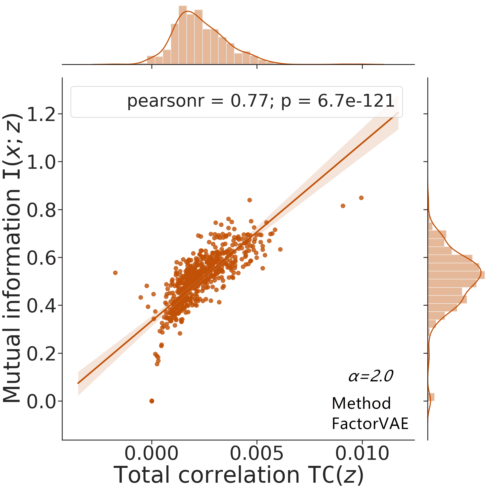
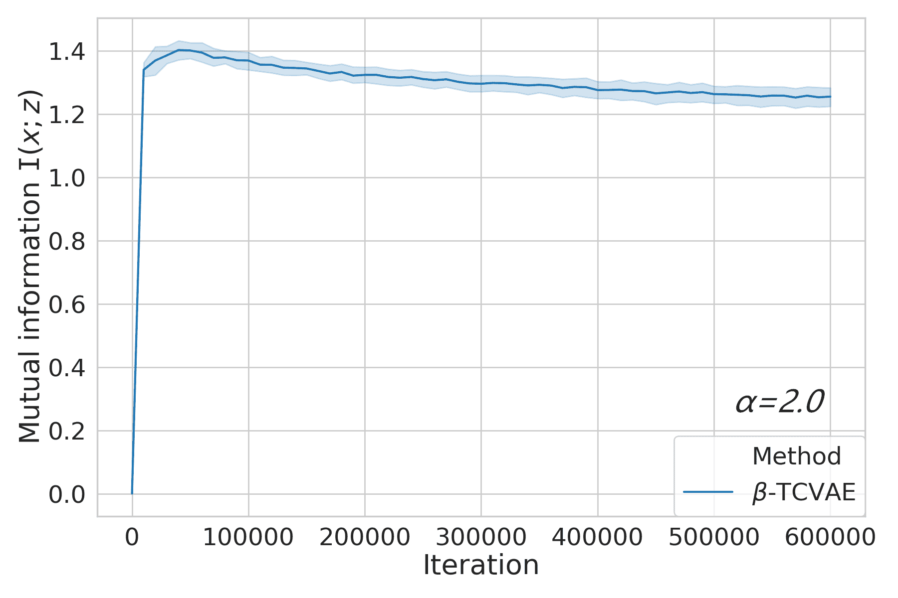
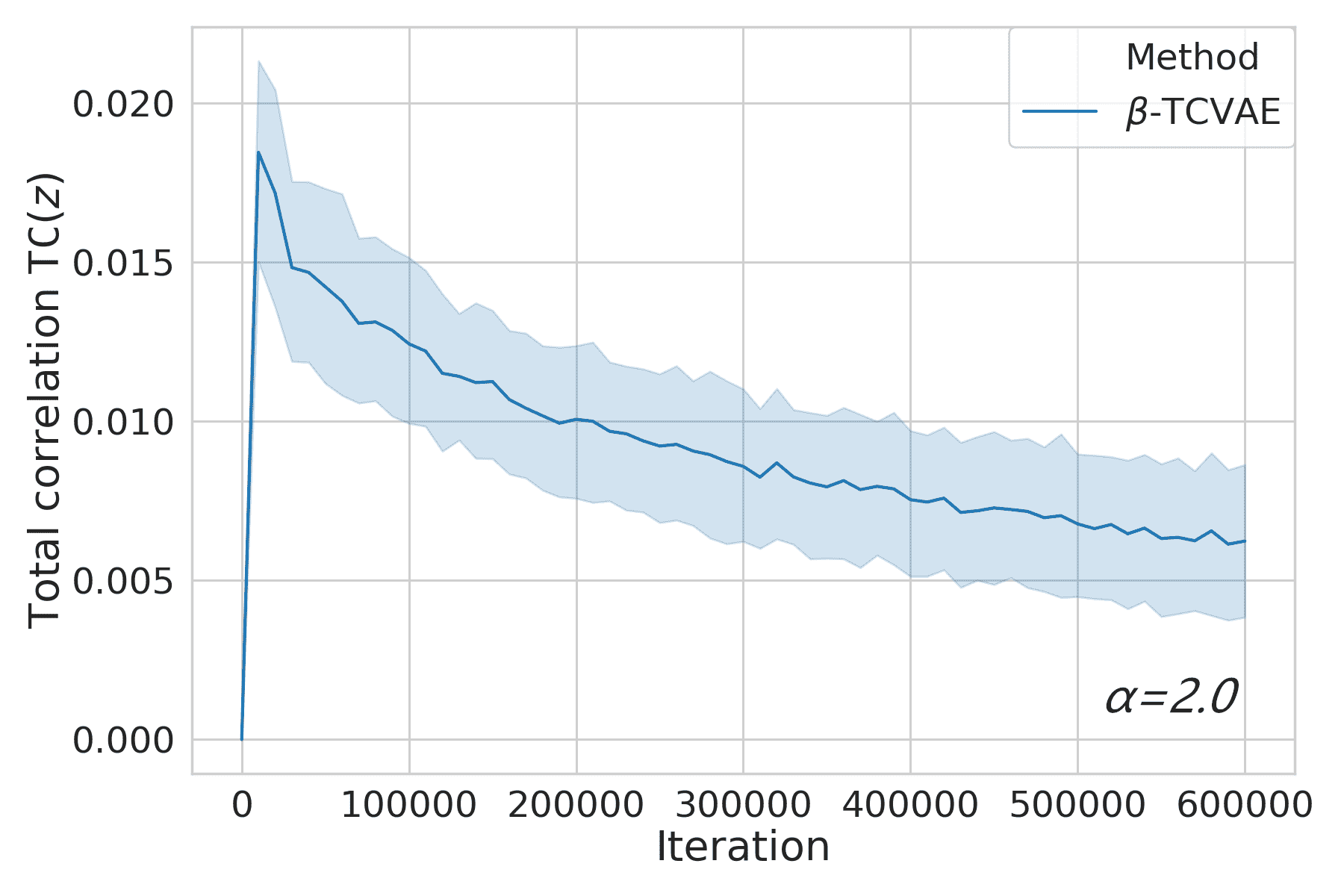
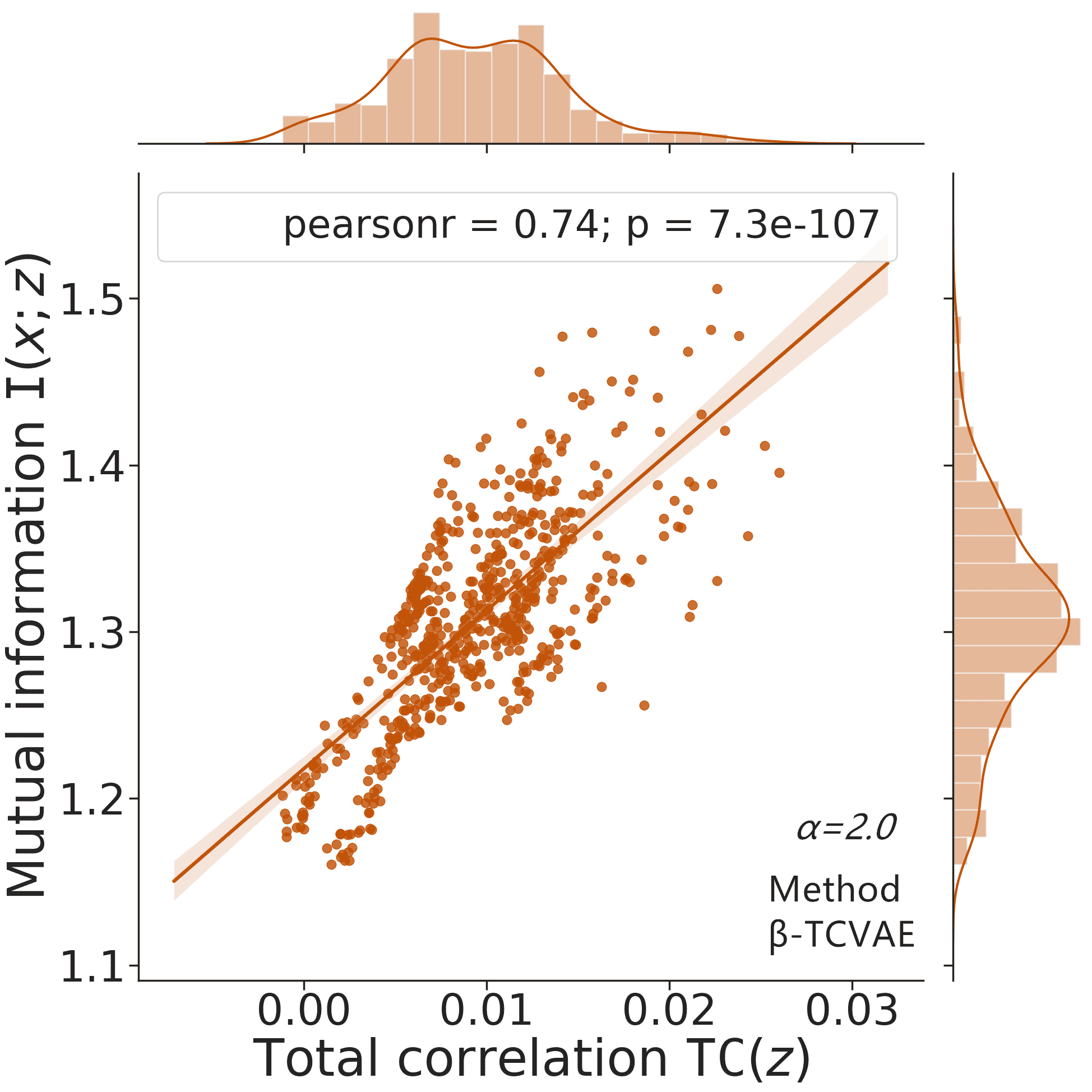
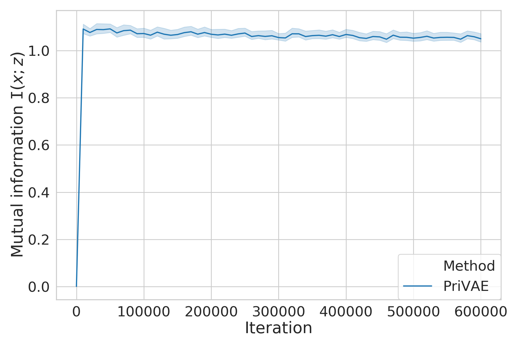
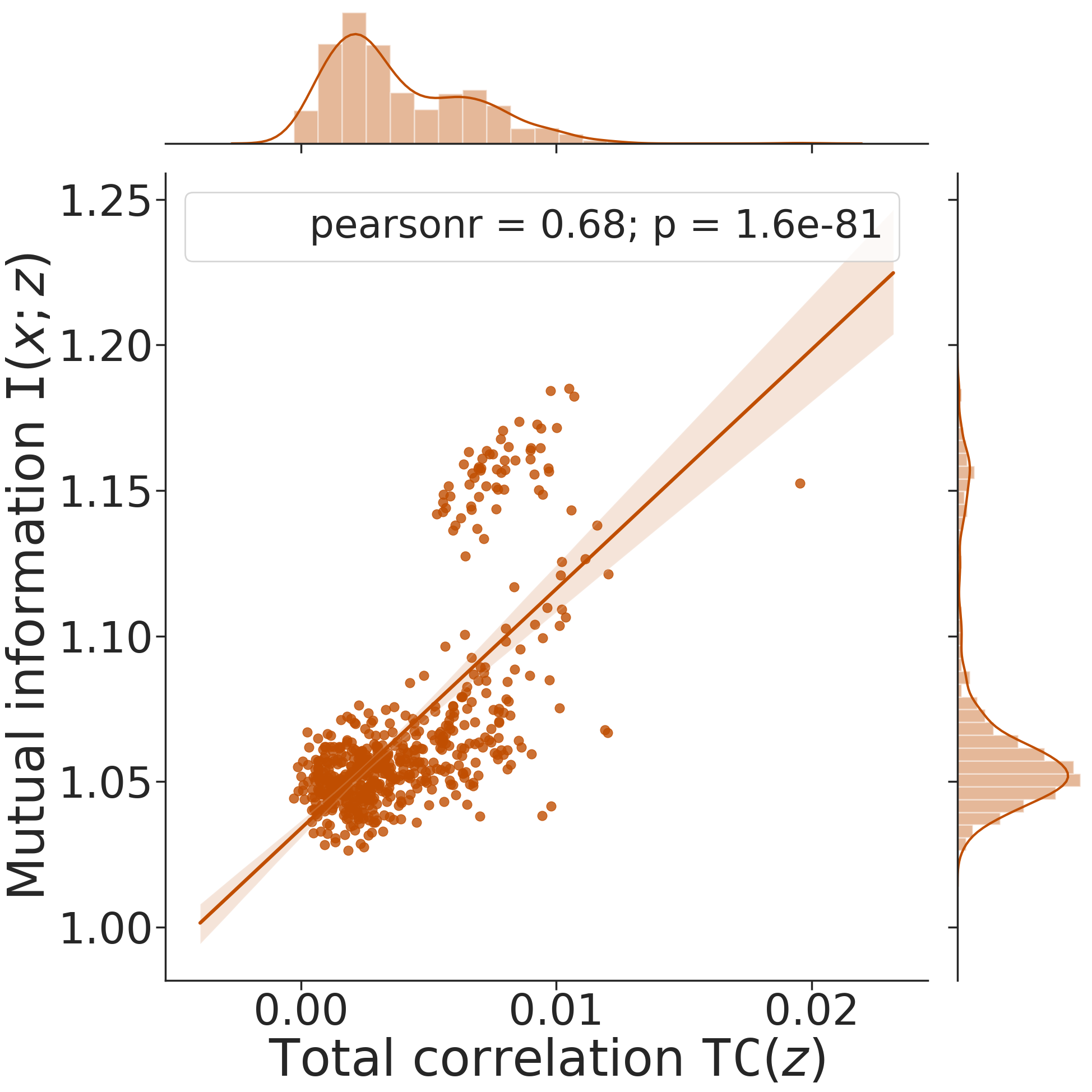
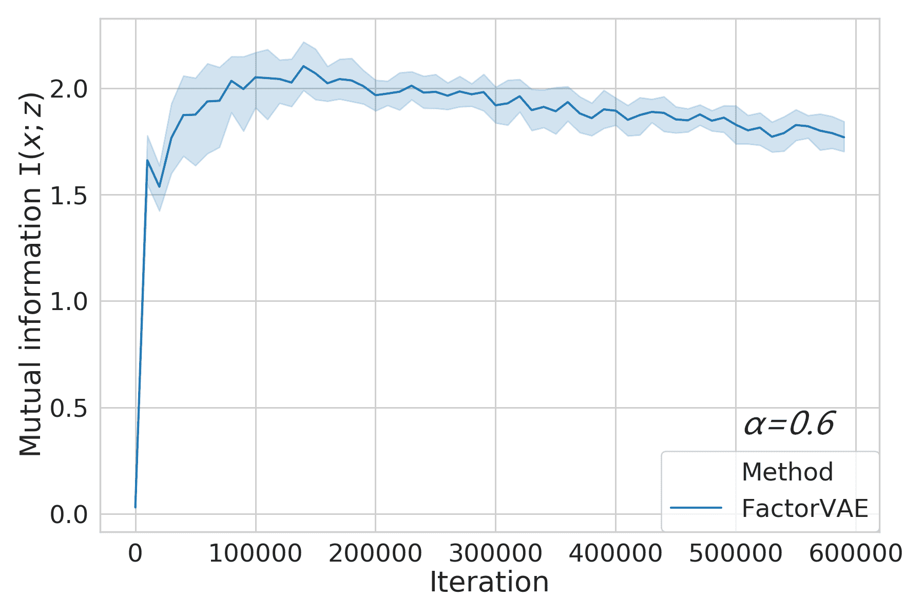
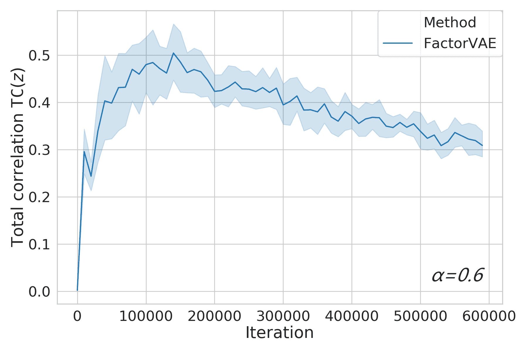
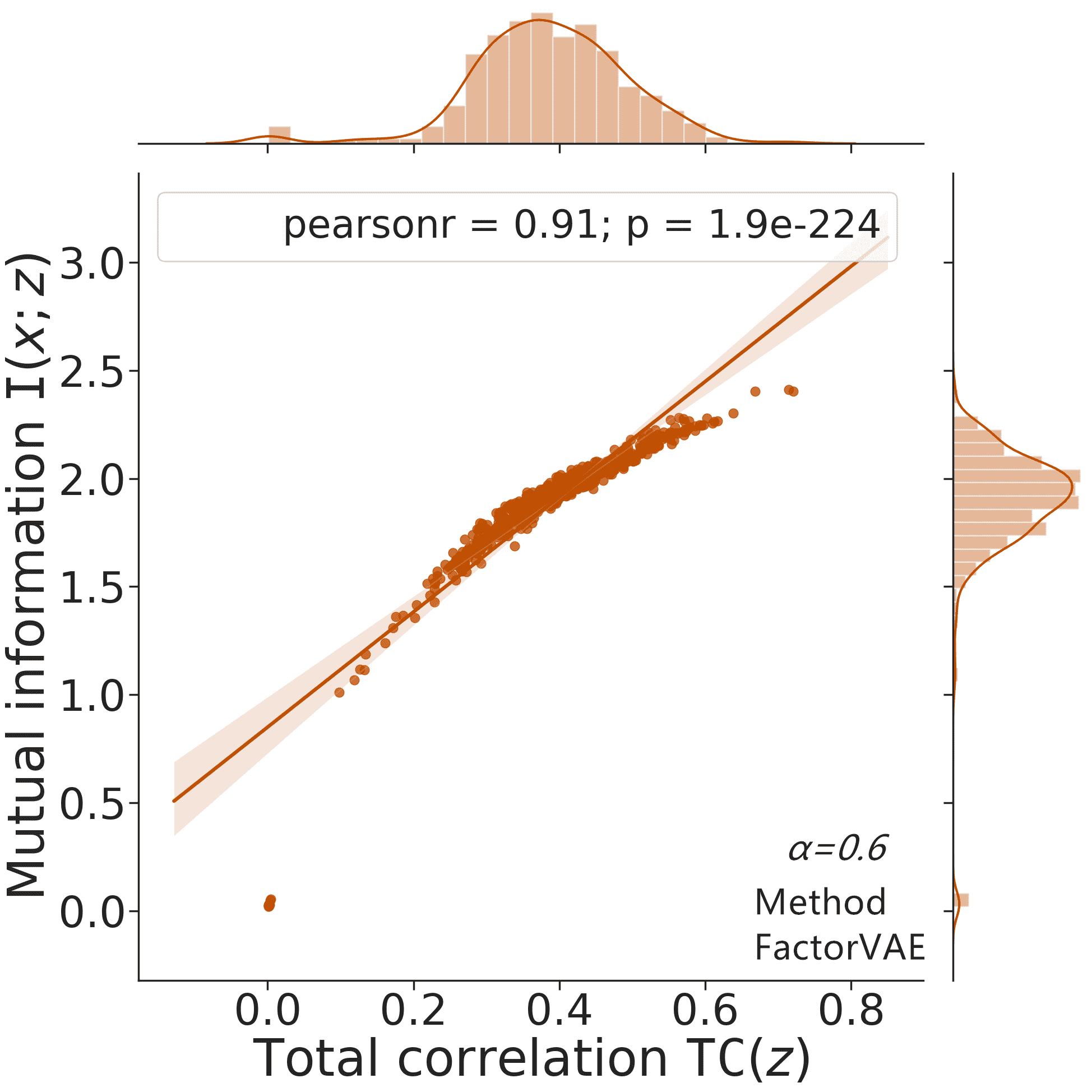
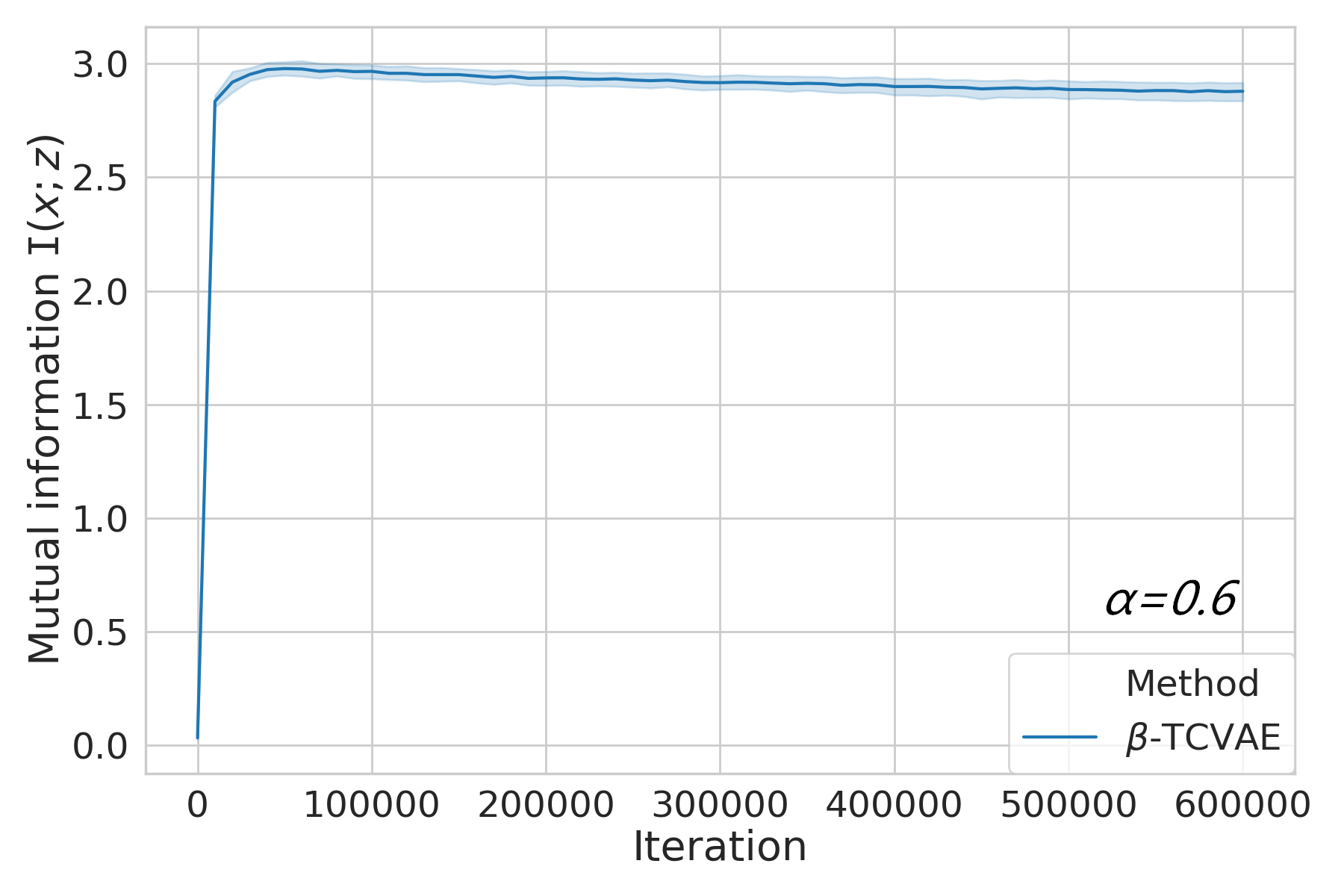
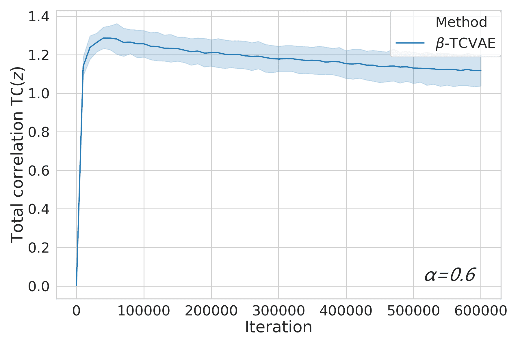
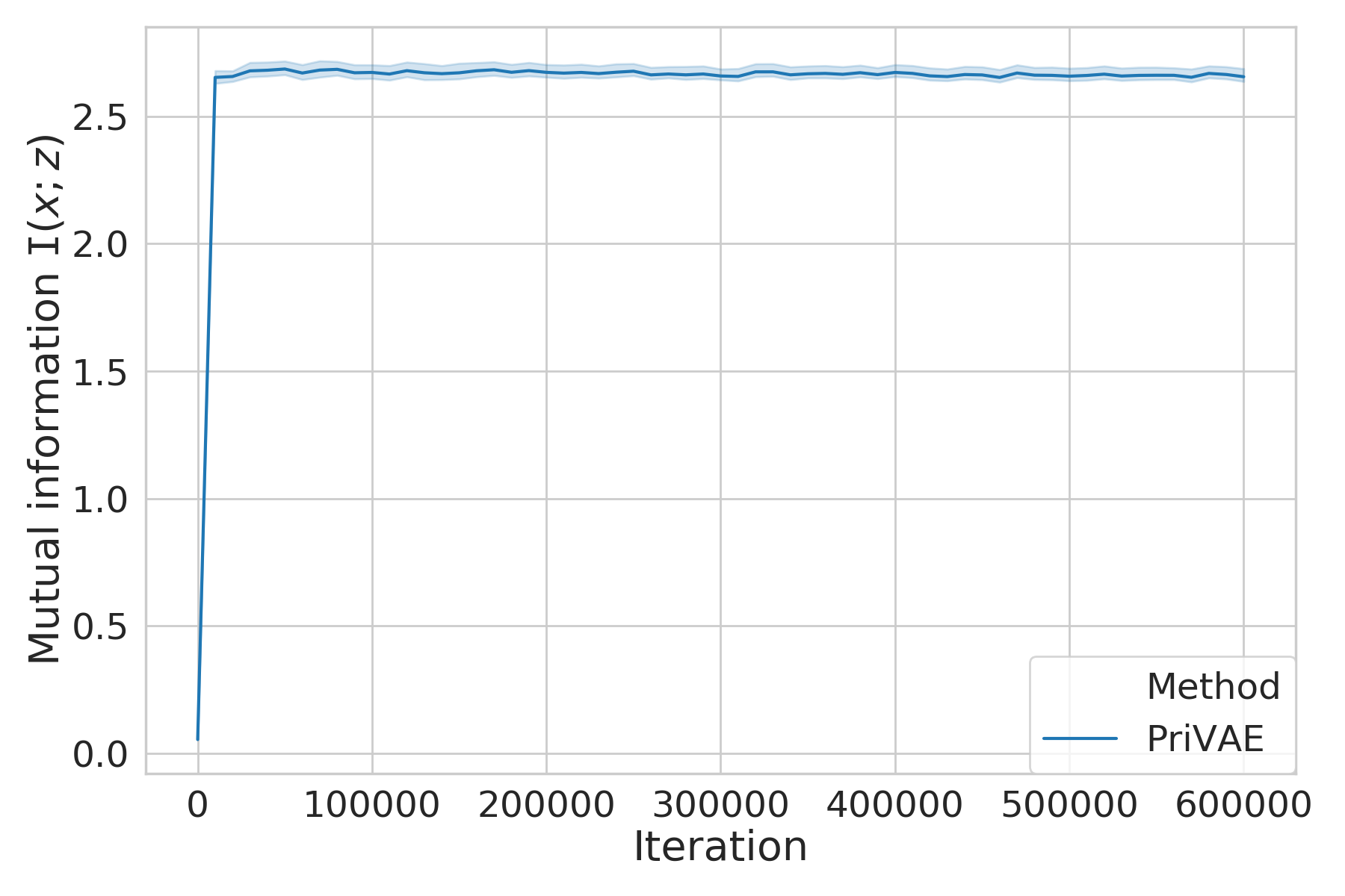
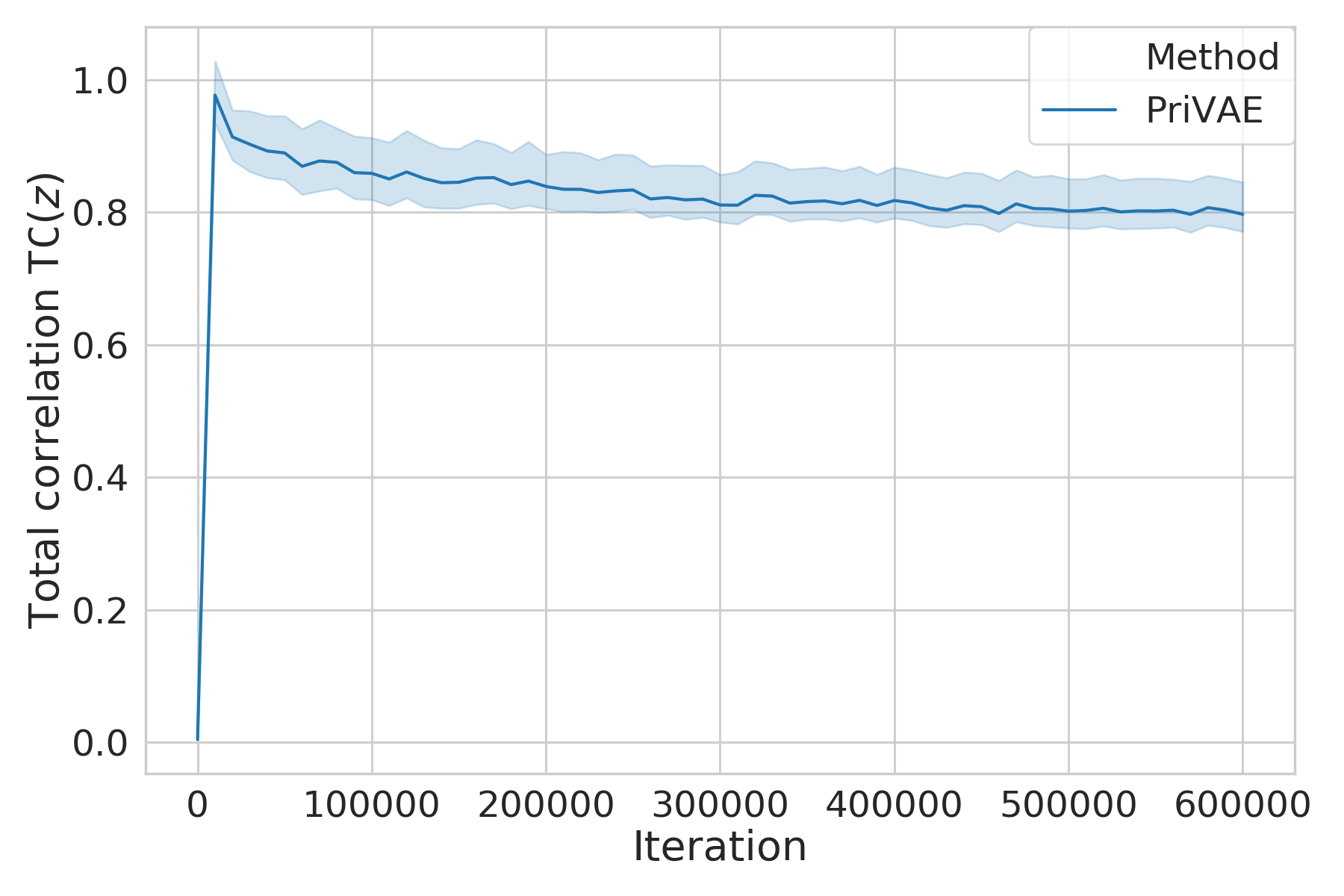
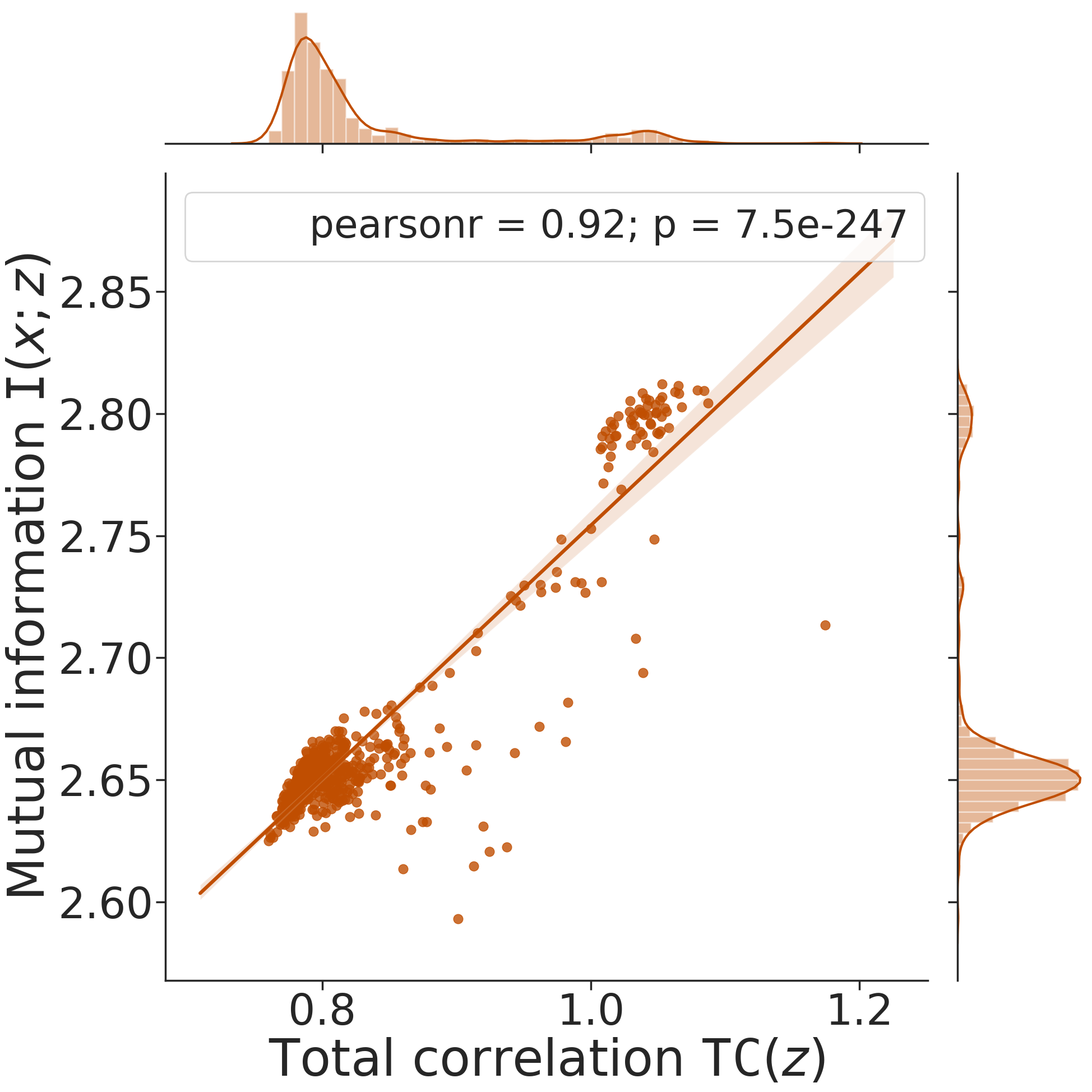
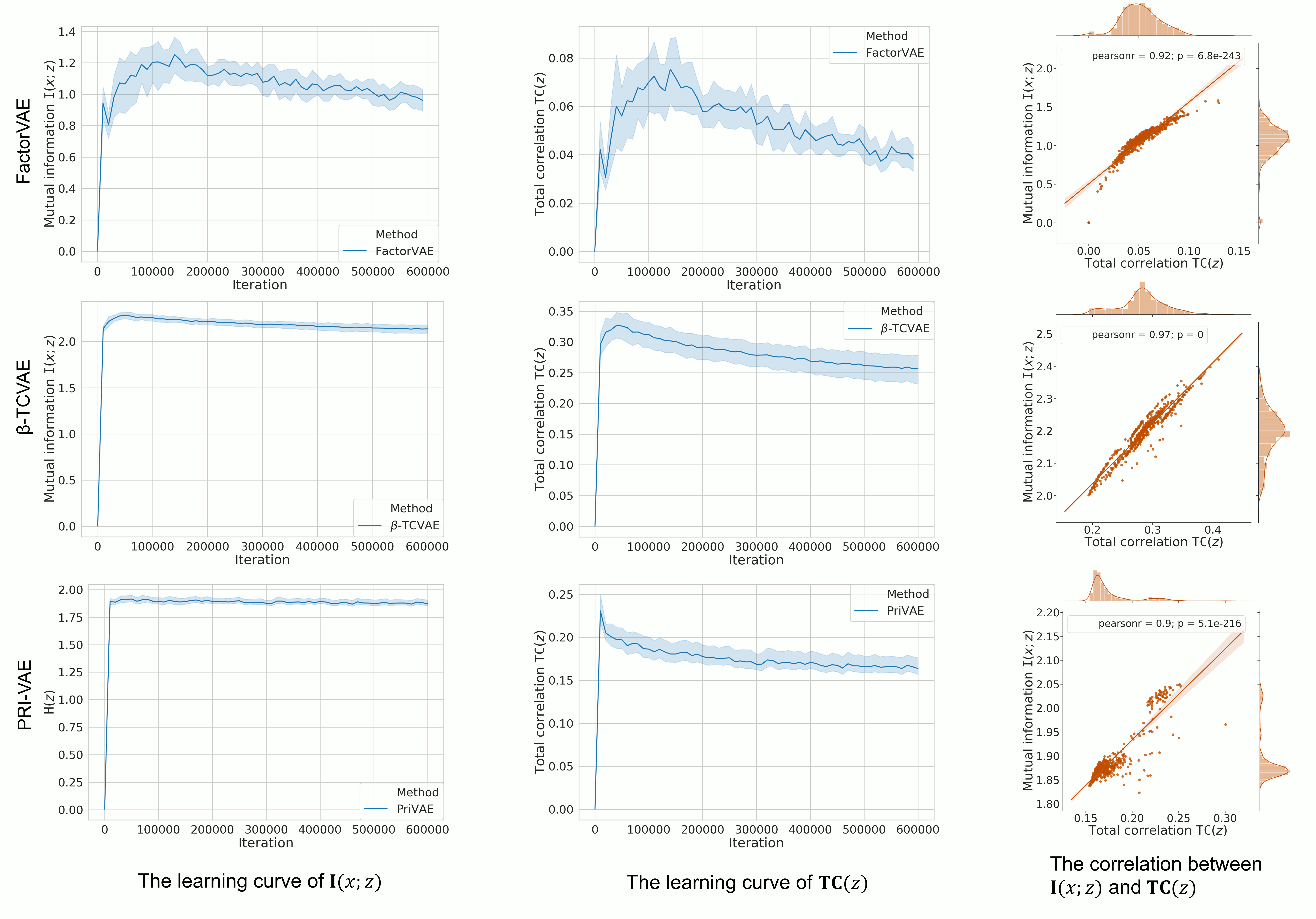
Fig. 2 demonstrates the evolution of 𝐈(𝐱;𝐳)𝐈𝐱𝐳\mathbf{I}(\mathbf{x};\mathbf{z}) and 𝐓(𝐳)𝐓𝐳\mathbf{T}(\mathbf{z}) for two representative VAEs across training iterations. Obviously, during the common SGD optimization, both 𝐈(𝐱;𝐳)𝐈𝐱𝐳\mathbf{I}(\mathbf{x};\mathbf{z}) and 𝐓(𝐳)𝐓𝐳\mathbf{T}(\mathbf{z}) show two separate phases: an early “fitting” phase, in which both 𝐈(𝐱;𝐭)𝐈𝐱𝐭\mathbf{I}(\mathbf{x};\mathbf{t}) and 𝐈(𝐭;𝐲)𝐈𝐭𝐲\mathbf{I}(\mathbf{t};\mathbf{y}) increase rapidly, and a later “compression” phase, in which there is a reversal such that 𝐈(𝐱;𝐭)𝐈𝐱𝐭\mathbf{I}(\mathbf{x};\mathbf{t}) and 𝐈(𝐭;𝐲)𝐈𝐭𝐲\mathbf{I}(\mathbf{t};\mathbf{y}) continually decrease. Our observation fits well with the arguments of the mainstream information theory community.

More interestingly, we also observe a significant positive correlation between 𝐈(𝐱;𝐳)𝐈𝐱𝐳\mathbf{I}(\mathbf{x};\mathbf{z}) and 𝐓(𝐳)𝐓𝐳\mathbf{T}(\mathbf{z}), as manifested by their Pearson correlation coefficient. Note that, a small value of 𝐓(𝐳)𝐓𝐳\mathbf{T}(\mathbf{z}) is always a good indicator to model disentanglement [7]. According to our observation, if 𝐓(𝐳)𝐓𝐳\mathbf{T}(\mathbf{z}) is optimized to a small value, 𝐈(𝐱;𝐳)𝐈𝐱𝐳\mathbf{I}(\mathbf{x};\mathbf{z}) should be small accordingly (even zero if fully disentangled). However, it is counter-intuitive that an extremely small value of 𝐈(𝐱;𝐳)𝐈𝐱𝐳\mathbf{I}(\mathbf{x};\mathbf{z}) is able to faithfully reconstruct the input [10, 7]. In this sense, our observation provides empirical evidence to support the argument in [36], which states that existing VAE models tend to learn uninformative latent representation. It also suggests there is always a trade-off between reconstruction and disentanglement [15, 9, 11].
Refer to caption
Figure 2: The evolution of the value of 𝐈(𝐱;𝐳)𝐈𝐱𝐳\mathbf{I}(\mathbf{x};\mathbf{z}) (left column) and the value of 𝐓(𝐳)𝐓𝐳\mathbf{T}(\mathbf{z}) (middle column) across training iterations for FactorVAE, β𝛽\beta-TCVAE and PRI-VAE on Cars3d data set. The right column shows the positive correlation between these two values.

IV-B Observations with Other Estimators

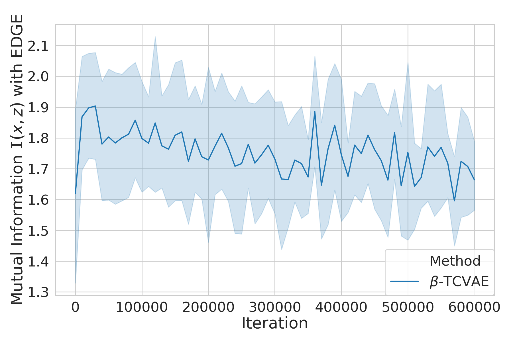
Our aim here is to verify if the general observation made by our suggested matrix-based Rényi’s α𝛼\alpha-entropy functional are consistent with other existing Shannon estimators. To this end, we estimate 𝐓(𝐳)𝐓𝐳\mathbf{T}(\mathbf{z}) with the widely used k𝑘kNN estimator [13] and kernel density estimator (KDE) [18]. We also apply the recently proposed ensemble dependency graph estimator (EDGE) [19] to measure 𝐈(𝐱;𝐳)𝐈𝐱𝐳\mathbf{I}(\mathbf{x};\mathbf{z}). Fig. 3 suggests that our general observation is in accordance with other popular estimators. However, note that both k𝑘kNN and KDE suffer from the curse of dimensionality, and it still remains a problem on estimating total correlation with EDGE.
Refer to caption
(a)
Refer to caption
(b)
Figure 3: The evolution of value of 𝐈(𝐱;𝐳)𝐈𝐱𝐳\mathbf{I}(\mathbf{x};\mathbf{z}) (left) measured by EDGE estimator and 𝐓(𝐳)𝐓𝐳\mathbf{T}(\mathbf{z}) (right) measured by k𝑘kNN and KDE.

V Experiments

We evaluate the performances of our proposed PRI-VAE on four benchmark data sets to demonstrate its capability to learn disentangled, interpretable latent representations, and reconstruct input signal with high fidelity. We compare PRI-VAE with six SOTA VAE models, namely β𝛽\beta-VAE [10], AnnealedVAE [5], DIP-VAE [14], InfoVAE [36], FactorVAE [11], and β𝛽\beta-TCVAE [7]. We evaluate the disentanglement and reconstruction performances of all competing models quantitatively (in Section V-A) and qualitatively (in Section V-B). We also illustrate the potential implications of our methodology for future work and generalize the idea of PRI-VAE to a higher level in Section V-C. For a fair comparison, all competing methods are trained with the same network architecture, optimizer, and mini-batch and evaluated by unified disentangling metrics [16].

V-A Quantitative Evaluation

We perform quantitative evaluation on dSprites [17] and Cars3D [24]. Samples in both data sets are generated with ground-truth independent latent factors. Since most of the existing metrics on disentanglement evaluation are positively correlated [16], we consider the most widely used Mutual Information Gap (MIG) [7] and DCI Disentanglement metric [26, 16] in this work.

V-A1 Comparison of PRI-VAE and InfoVAE Family

The most similar objective to PRI-VAE is the InfoVAE family [36] with the regularization term α1+λ2𝛼1𝜆2\alpha\leavevmode\hbox to9.75pt{\vbox to9.75pt{\pgfpicture\makeatletter\hbox{\hskip 4.87285pt\lower-4.87285pt\hbox to0.0pt{\pgfsys@beginscope\pgfsys@invoke{ }\definecolor{pgfstrokecolor}{rgb}{0,0,0}\pgfsys@color@rgb@stroke{0}{0}{0}\pgfsys@invoke{ }\pgfsys@color@rgb@fill{0}{0}{0}\pgfsys@invoke{ }\pgfsys@setlinewidth{0.4pt}\pgfsys@invoke{ }\nullfont\hbox to0.0pt{\pgfsys@beginscope\pgfsys@invoke{ }{{{}}\hbox{\hbox{{\pgfsys@beginscope\pgfsys@invoke{ }{{}{{{}}}{{}}{}{}{}{}{}{}{}{}{}{{}\pgfsys@moveto{4.67285pt}{0.0pt}\pgfsys@curveto{4.67285pt}{2.58076pt}{2.58076pt}{4.67285pt}{0.0pt}{4.67285pt}\pgfsys@curveto{-2.58076pt}{4.67285pt}{-4.67285pt}{2.58076pt}{-4.67285pt}{0.0pt}\pgfsys@curveto{-4.67285pt}{-2.58076pt}{-2.58076pt}{-4.67285pt}{0.0pt}{-4.67285pt}\pgfsys@curveto{2.58076pt}{-4.67285pt}{4.67285pt}{-2.58076pt}{4.67285pt}{0.0pt}\pgfsys@closepath\pgfsys@moveto{0.0pt}{0.0pt}\pgfsys@stroke\pgfsys@invoke{ } }{{{{}}\pgfsys@beginscope\pgfsys@invoke{ }\pgfsys@transformcm{1.0}{0.0}{0.0}{1.0}{-2.0pt}{-2.57777pt}\pgfsys@invoke{ }\hbox{{\definecolor{pgfstrokecolor}{rgb}{0,0,0}\pgfsys@color@rgb@stroke{0}{0}{0}\pgfsys@invoke{ }\pgfsys@color@rgb@fill{0}{0}{0}\pgfsys@invoke{ }\hbox{{\footnotesize 1}} }}\pgfsys@invoke{\lxSVG@closescope }\pgfsys@endscope}}} \pgfsys@invoke{\lxSVG@closescope }\pgfsys@endscope}}} } \pgfsys@invoke{\lxSVG@closescope }\pgfsys@endscope{{{}}}{}{}\hss}\pgfsys@discardpath\pgfsys@invoke{\lxSVG@closescope }\pgfsys@endscope\hss}}\lxSVG@closescope\endpgfpicture}}+\lambda\leavevmode\hbox to9.75pt{\vbox to9.75pt{\pgfpicture\makeatletter\hbox{\hskip 4.87285pt\lower-4.87285pt\hbox to0.0pt{\pgfsys@beginscope\pgfsys@invoke{ }\definecolor{pgfstrokecolor}{rgb}{0,0,0}\pgfsys@color@rgb@stroke{0}{0}{0}\pgfsys@invoke{ }\pgfsys@color@rgb@fill{0}{0}{0}\pgfsys@invoke{ }\pgfsys@setlinewidth{0.4pt}\pgfsys@invoke{ }\nullfont\hbox to0.0pt{\pgfsys@beginscope\pgfsys@invoke{ }{{{}}\hbox{\hbox{{\pgfsys@beginscope\pgfsys@invoke{ }{{}{{{}}}{{}}{}{}{}{}{}{}{}{}{}{{}\pgfsys@moveto{4.67285pt}{0.0pt}\pgfsys@curveto{4.67285pt}{2.58076pt}{2.58076pt}{4.67285pt}{0.0pt}{4.67285pt}\pgfsys@curveto{-2.58076pt}{4.67285pt}{-4.67285pt}{2.58076pt}{-4.67285pt}{0.0pt}\pgfsys@curveto{-4.67285pt}{-2.58076pt}{-2.58076pt}{-4.67285pt}{0.0pt}{-4.67285pt}\pgfsys@curveto{2.58076pt}{-4.67285pt}{4.67285pt}{-2.58076pt}{4.67285pt}{0.0pt}\pgfsys@closepath\pgfsys@moveto{0.0pt}{0.0pt}\pgfsys@stroke\pgfsys@invoke{ } }{{{{}}\pgfsys@beginscope\pgfsys@invoke{ }\pgfsys@transformcm{1.0}{0.0}{0.0}{1.0}{-2.0pt}{-2.57777pt}\pgfsys@invoke{ }\hbox{{\definecolor{pgfstrokecolor}{rgb}{0,0,0}\pgfsys@color@rgb@stroke{0}{0}{0}\pgfsys@invoke{ }\pgfsys@color@rgb@fill{0}{0}{0}\pgfsys@invoke{ }\hbox{{\footnotesize 2}} }}\pgfsys@invoke{\lxSVG@closescope }\pgfsys@endscope}}} \pgfsys@invoke{\lxSVG@closescope }\pgfsys@endscope}}} } \pgfsys@invoke{\lxSVG@closescope }\pgfsys@endscope{{{}}}{}{}\hss}\pgfsys@discardpath\pgfsys@invoke{\lxSVG@closescope }\pgfsys@endscope\hss}}\lxSVG@closescope\endpgfpicture}}. Despite reaching similar objectives, the routes to this result are rather different. Our PRI-VAE is motivated by an information-theoretic perspective in the sense that we want to learn a compact (regularized by α𝐇(𝐳)𝛼𝐇𝐳\alpha\mathbf{H}(\mathbf{z})) latent representation that is able to reconstruct input signal (regularized by 𝔼p(𝐱)[𝔼q(𝐳|𝐱)[logp(𝐱|𝐳)]]subscript𝔼𝑝𝐱delimited-[]subscript𝔼𝑞conditional𝐳𝐱delimited-[]𝑝conditional𝐱𝐳\mathbb{E}_{p(\mathbf{x})}\left[\mathbb{E}_{q(\mathbf{z}|\mathbf{x})}\left[\log p(\mathbf{x}|\mathbf{z})\right]\right]) and is also disentangled (regularized by βDKL[qϕ(𝐳)p(𝐳)]𝛽subscript𝐷𝐾𝐿delimited-[]conditionalsubscript𝑞italic-ϕ𝐳𝑝𝐳\beta D_{KL}[q_{\phi}(\mathbf{z})\|p(\mathbf{z})]). By contrast, InfoVAE family originates from a generative model perspective that attempts to address two fundamental issues in the original VAE (i.e., the inaccurate amortized inference distributions and the vanishing relevance of latent variable and input signal). Although authors of InfoVAE suggest setting α=0𝛼0\alpha=0 to completely drop 1, we demonstrate here the superiority gained from the difference, i.e., α(𝐇(𝐳)𝐈(𝐱;𝐳))𝛼𝐇𝐳𝐈𝐱𝐳\alpha(\mathbf{H}(\mathbf{z})-\mathbf{I}(\mathbf{x};\mathbf{z})).

Refer to caption
(a)
Refer to caption
(b)
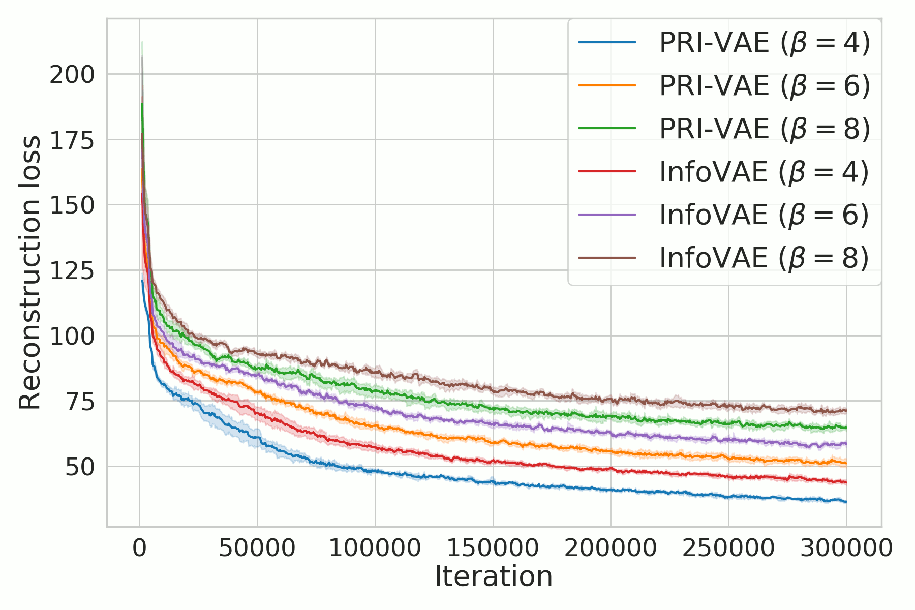
Figure 4: The evolutions of MIG score (left) and reconstruction loss (right, after exponential moving average with weight 0.80.80.8) for PRI-VAE and InfoVAE family with respect to different values of α𝛼\alpha when β𝛽\beta is fixed to 444.
Refer to caption
(a)
Refer to caption
(b)
Figure 5: The evolutions of MIG score (left) and reconstruction loss (right, after exponential moving average with weight 0.80.80.8) for PRI-VAE and InfoVAE family with respect to different values of β𝛽\beta when α𝛼\alpha is fixed to 111.

We first evaluate the performances of PRI-VAE and InfoVAE family with respect to different values of α𝛼\alpha by fixing β=4𝛽4\beta=4 (a common setting in previous works [10, 9]). Fig. 4 demonstrates the evolution of the MIG score and the reconstruction loss across training iterations on dSprites data set. Under the same hyper-parameter setting (i.e., same value of α𝛼\alpha), PRI-VAE can quickly obtain more disentangled latent representation with smaller reconstruction error than its InfoVAE counterpart. This is not surprising. Note that 𝐇(𝐳)𝐈(𝐱;𝐳)0𝐇𝐳𝐈𝐱𝐳0\mathbf{H}(\mathbf{z})-\mathbf{I}(\mathbf{x};\mathbf{z})\geq 0, i.e., 𝐇(𝐳)𝐇𝐳\mathbf{H}(\mathbf{z}) is always a heavy penalty than 𝐈(𝐱;𝐳)𝐈𝐱𝐳\mathbf{I}(\mathbf{x};\mathbf{z}). Therefore, a faster convergence is expected.

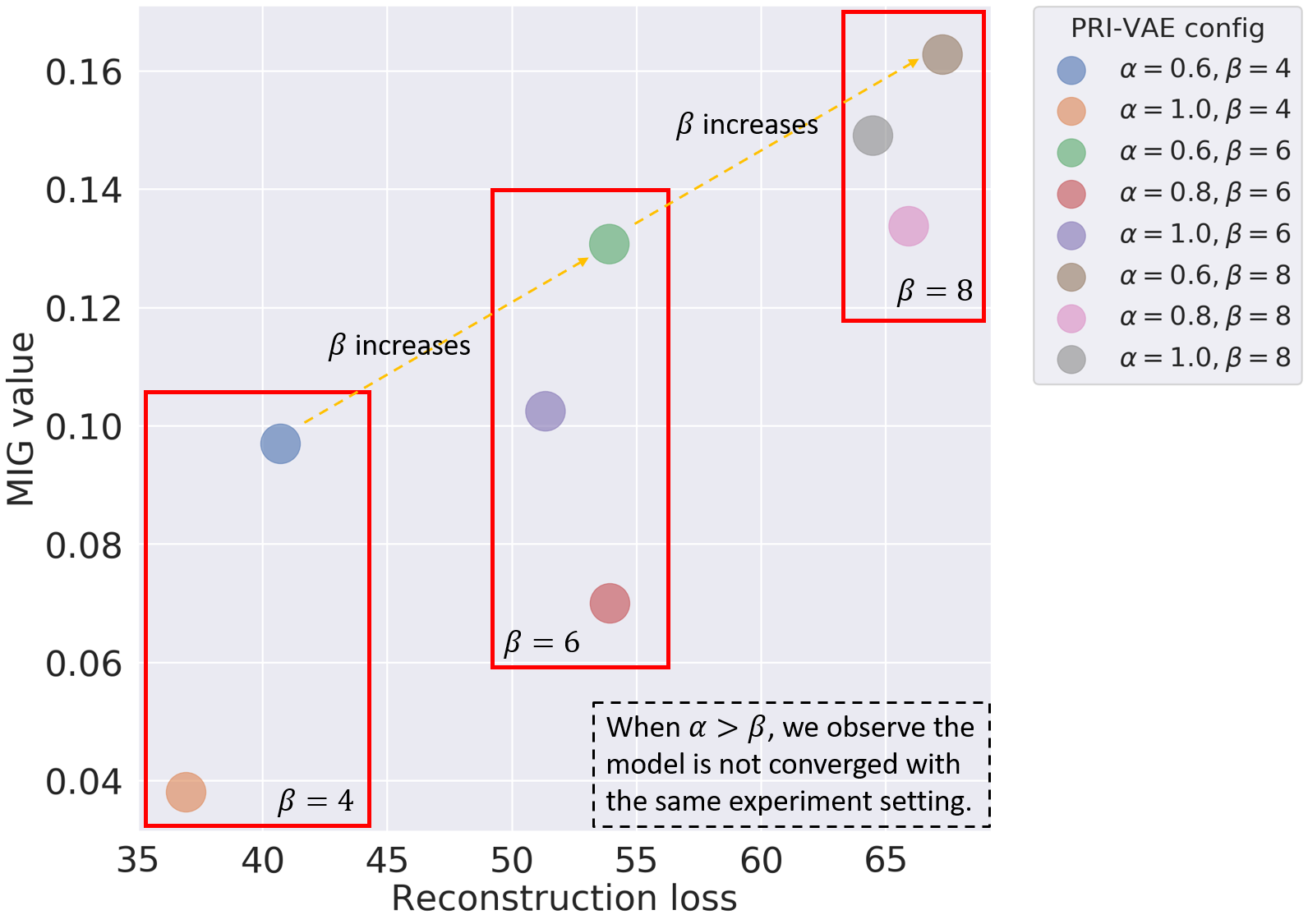
Fig. 5 reaffirms the advantage of PRI-VAE over InfoVAE family concerning different values of β𝛽\beta. Another interesting observation is that, with the increase of β𝛽\beta, the MIG score keeps increasing, whereas the reconstruction quality is reduced. This is probably because there is a trade-off between reconstruction and disentanglement [15, 11, 9].

V-A2 Comparison of PRI-VAE and other SOTA VAE Models

Next, we compare PRI-VAE with VAE, β𝛽\beta-VAE, AnnealedVAE, DIP-VAE-I, DIP-VAE-II, FactorVAE and β𝛽\beta-TCVAE. As recommended in [16], we finalize the hyperparameters for each methods by sweeping over a wide enough regularization weight range. We then fix the hyperparameters of all methods on different data sets. Specifically, we select β=4𝛽4\beta=4 for β𝛽\beta-VAE and β𝛽\beta-TCVAE, γ=30𝛾30\gamma=30 for FactorVAE, λod=5subscript𝜆𝑜𝑑5\lambda_{od}=5, λd=10λodsubscript𝜆𝑑10subscript𝜆𝑜𝑑\lambda_{d}=10\lambda_{od} for DIP-VAE-I and λod=5subscript𝜆𝑜𝑑5\lambda_{od}=5, λd=λodsubscript𝜆𝑑subscript𝜆𝑜𝑑\lambda_{d}=\lambda_{od} for DIP-VAE-II. For AnnealedVAE, we fix γ=1000𝛾1000\gamma=1000 and linearly increase the channel capacity C𝐶C from 00 to 252525 over the course of 10,0001000010,000 training steps. For our model, we select α=0.6𝛼0.6\alpha=0.6 and β=6.0𝛽6.0\beta=6.0111We recommend β2α𝛽2𝛼\beta\geq 2\alpha. This is because 𝐳𝐳\mathbf{z} converges to a single point if βα𝛽𝛼\beta\leq\alpha (see Fig. 1), from which it is hard to reconstruct 𝐱𝐱\mathbf{x}.. Ten independent runs are performed.
Refer to caption
(a)
Refer to caption
(b)
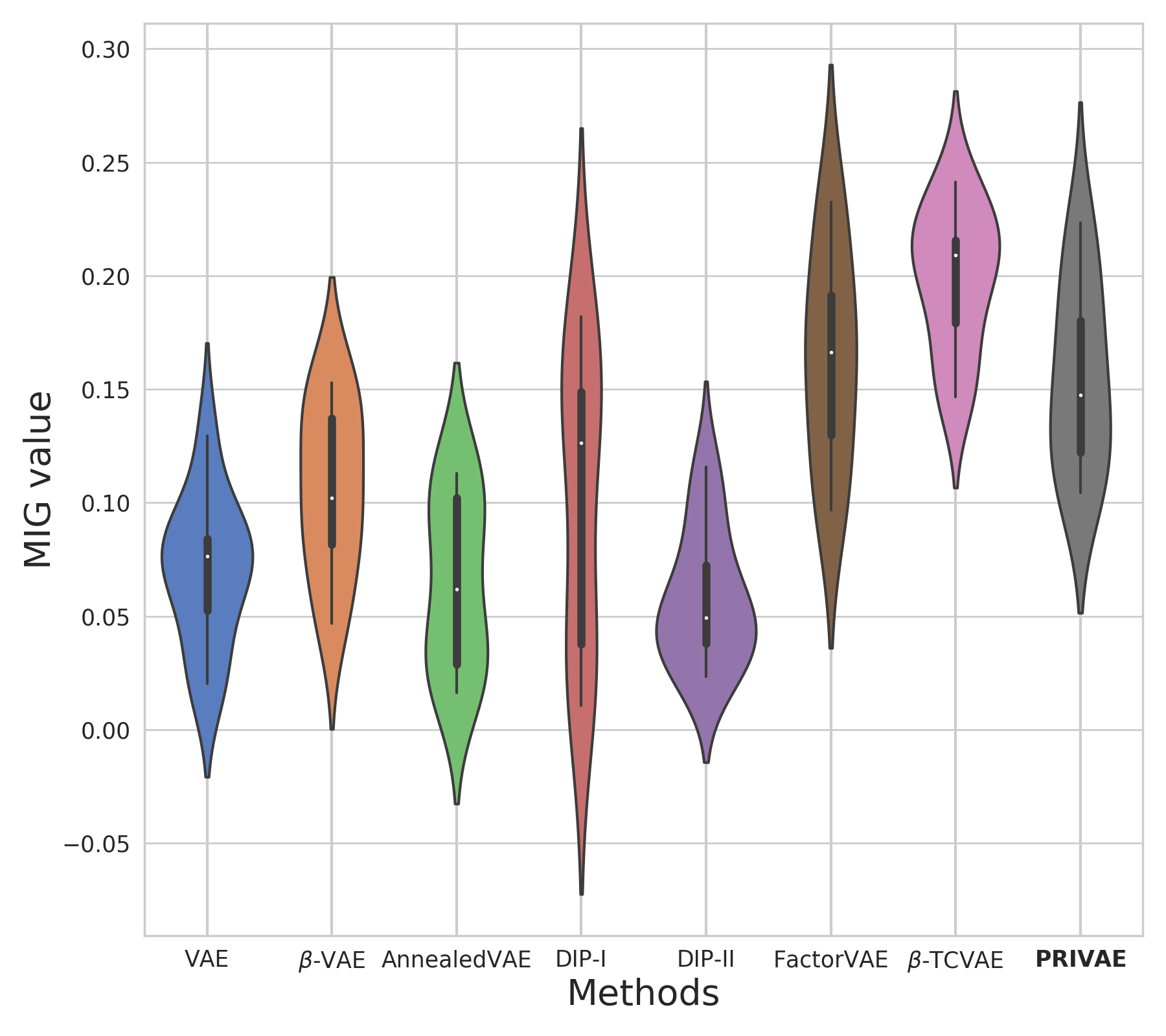
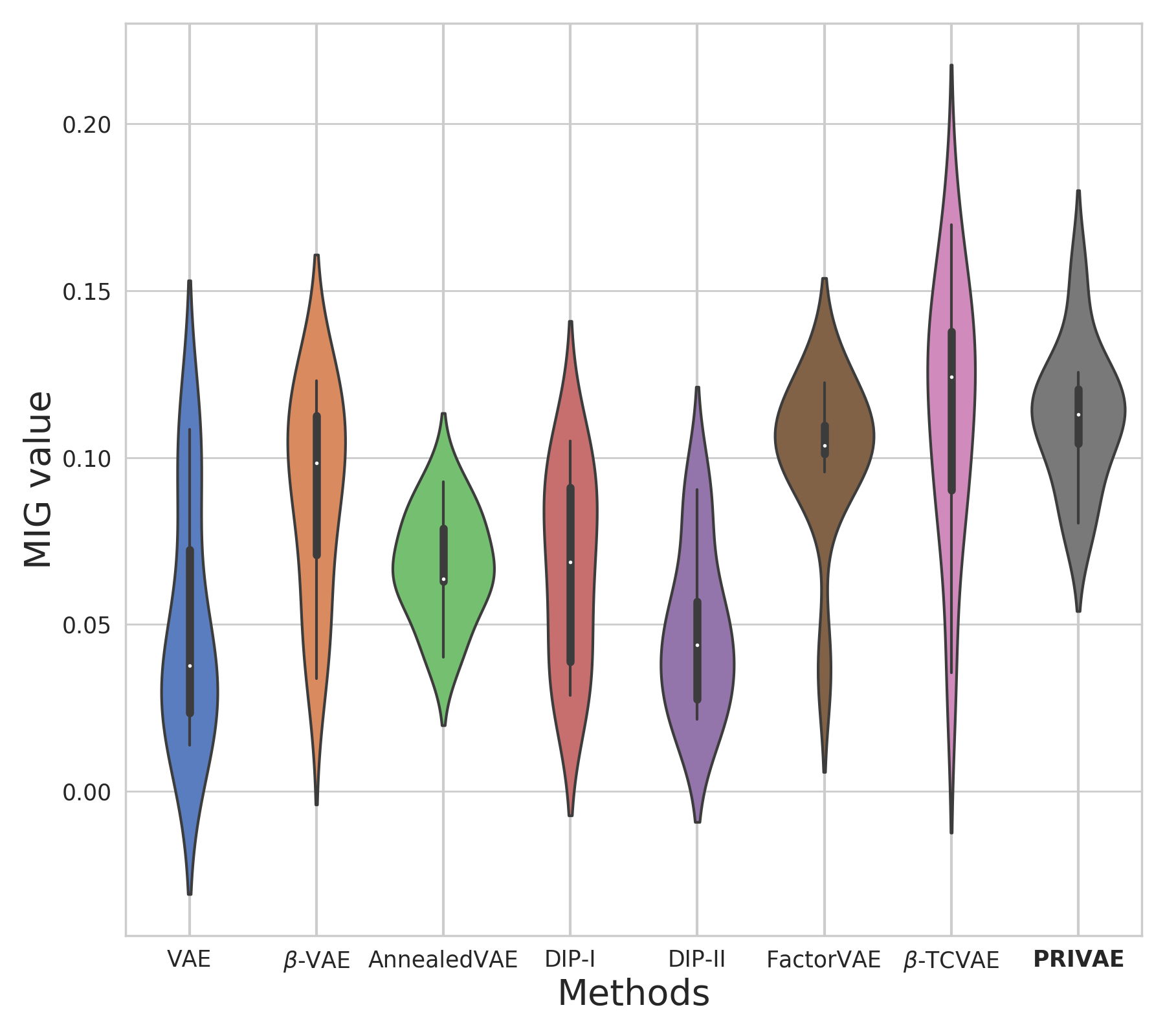
Figure 6: The MIG score comparison on dSprites (left) and Cars3D (right) data sets.

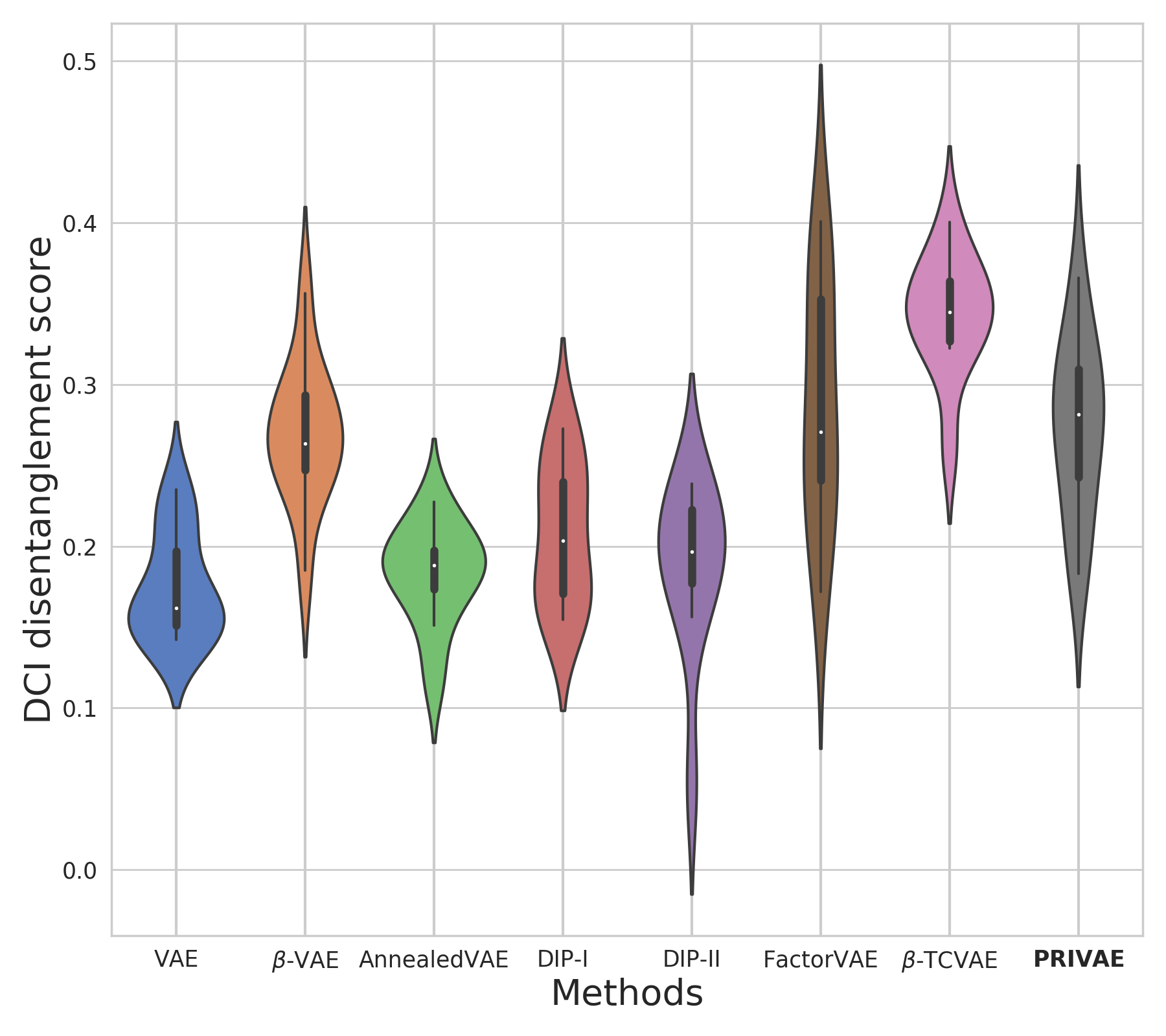
Fig. 6 demonstrates the MIG score for all competing models in dSprites and Cars3D, respectively222Same to [16, 9], we also observe that the hyper-parameter tuning and the random seed have substantial impacts to the performances of different models.. The comparison result on DCI disentanglement metric is similar, which is shown in Appendix Fig. C3. As can be seen, PRI-VAE achieves consistent better disentanglement performance than VAE, β𝛽\beta-VAE, AnnealedVAE, and DPI-VAE, and preserves a satisfactory reconstruction quality suggested by our visualization results (see Appendix Fig. C5). However, β𝛽\beta-TCVAE and FactorVAE obtain higher disentanglement scores than ours. This is not surprising. Both FactorVAE and β𝛽\beta-TCVAE add a new regularization term 𝐓(𝐳)𝐓𝐳\mathbf{T}(\mathbf{z}) with extra weight to the original VAE objective. One should note that 𝐓(𝐳)𝐓𝐳\mathbf{T}(\mathbf{z}) is always a more explicit and heavy penalty than DKL(qϕ(𝐳)p(𝐳))subscript𝐷𝐾𝐿conditionalsubscript𝑞italic-ϕ𝐳𝑝𝐳D_{KL}(q_{\phi}(\mathbf{z})\|p(\mathbf{z})) to encourage independence of each dimension of 𝐳𝐳\mathbf{z} [7]. We will show in Section V-C1 that the merits of PRI-VAE and β𝛽\beta-TCVAE can be merged to significantly improve the performances of both methods.

V-B Qualitative Evaluation

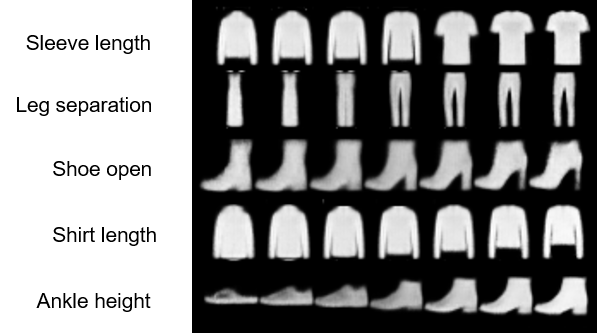
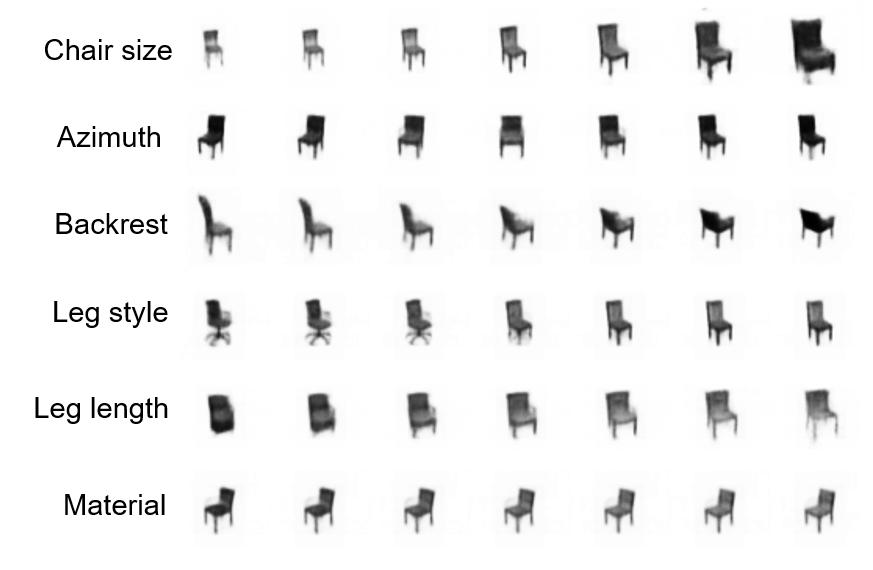
We then quantitatively evaluate PRI-VAE on 3D Chairs [3], and Fashion-MNIST [32]. Fig. 7 and Fig. 8 show the traversal results of the latent variables on both data sets, respectively. Similar to β𝛽\beta-TCVAE, PRI-VAE is able to discover six factors of variation in 3D Chairs, such as chair size, azimuth, backrest, leg style, leg length, and chair material. By contrast, β𝛽\beta-VAE can only learn four factors [7]. Moreover, PRI-VAE discovers a unique factor (i.e., leg separation) in Fashion-MNIST, which has never been mentioned in previous works.
Refer to caption
Figure 7: Latent traversals for the PRI-VAE (α=0.6,β=4formulae-sequence𝛼0.6𝛽4\alpha=0.6,\beta=4) trained on 3D chairs. Each column corresponds to varying a single latent unit. The traversal is over the [2,2]22[-2,2] range.
Refer to caption
Figure 8: Latent traversals for the PRI-VAE (α=0.6,β=8formulae-sequence𝛼0.6𝛽8\alpha=0.6,\beta=8) trained on Fashion-MNIST. Each column corresponds to varying a single latent unit. The traversal is over the [3,3]33[-3,3] range.

V-C Implications for Future Work

We finally present two positive implications of our methodology for future work with convincing empirical validation.

V-C1 Merging the Merits of PRI-VAE and β𝛽\beta-TCVAE

We continue our discussion in Section V-A2 to demonstrate the benefits gained from merging the merits of PRI-VAE and β𝛽\beta-TCVAE. As discussed earlier, FactorVAE and β𝛽\beta-TCVAE have better disentanglement performance than others by explicitly regularizing an extra term 𝐓(𝐳)𝐓𝐳\mathbf{T}(\mathbf{z}). On the other hand, the PRI is geometrically interpretable and enables faster convergence. Therefore, a natural idea to combine the merits of both methodologies is via the following objective:

PRIVAE=𝔼p(𝐱)[𝔼q(𝐳|𝐱)[logp(𝐱|𝐳)]]αH(𝐳)βDKL[q(𝐳)p(𝐳)]γDKL(q(𝐳)jq(𝐳j)).subscriptPRIsuperscriptVAEsubscript𝔼𝑝𝐱delimited-[]subscript𝔼𝑞conditional𝐳𝐱delimited-[]𝑝conditional𝐱𝐳𝛼𝐻𝐳𝛽subscript𝐷𝐾𝐿delimited-[]conditional𝑞𝐳𝑝𝐳𝛾subscript𝐷𝐾𝐿conditional𝑞𝐳subscriptproduct𝑗𝑞subscript𝐳𝑗\begin{split}&\mathcal{L}_{\mathrm{PRI}-\mathrm{VAE}^{\star}}\\ &=\mathbb{E}_{p(\mathbf{x})}\left[\mathbb{E}_{q(\mathbf{z}|\mathbf{x})}\left[\log p(\mathbf{x}|\mathbf{z})\right]\right]-\alpha H(\mathbf{z})\\ &-\beta D_{KL}[q(\mathbf{z})\|p(\mathbf{z})]-\gamma D_{KL}(q(\mathbf{z})\|\prod_{j}q\left(\mathbf{z}_{j}\right)).\end{split} (9)

We term Eq. (9) PRI-VAE since it just adds a weighted term γ𝐓(𝐳)𝛾𝐓𝐳\gamma\mathbf{T}(\mathbf{z}) to the original PRI-VAE objective. In Eq. (9), the term αH(𝐳)+βDKLq(𝐳)||p(𝐳))\alpha H(\mathbf{z})+\beta D_{KL}q(\mathbf{z})||p(\mathbf{z})) can be interpreted as an upper bound of the exact information rate 𝐈(𝐱;𝐳)𝐈𝐱𝐳\mathbf{I}(\mathbf{x};\mathbf{z}), whereas the new regularization term γDKL(q(𝐳)jq(𝐳j))𝛾subscript𝐷𝐾𝐿conditional𝑞𝐳subscriptproduct𝑗𝑞subscript𝐳𝑗\gamma D_{KL}(q(\mathbf{z})\|\prod_{j}q\left(\mathbf{z}_{j}\right)) further enforces the disentanglement. This way, we are actually optimizing a regularized rate-distortion problem. Given that minimizing 𝐓(𝐳)𝐓𝐳\mathbf{T}(\mathbf{z}) is likely to incur the decrease of 𝐈(𝐱;𝐳)𝐈𝐱𝐳\mathbf{I}(\mathbf{x};\mathbf{z}), the distortion may increase accordingly.

We compare PRI-VAE with PRI-VAE and β𝛽\beta-TCVAE on dSprites and Cars3D. We keep the same hyper-parameter setting for PRI-VAE and β𝛽\beta-TCVAE as shown in Section V-A2. For PRI-VAE, we set α=0.5,β=1.0formulae-sequence𝛼0.5𝛽1.0\alpha=0.5,\beta=1.0 and γ=4.0𝛾4.0\gamma=4.0. Table II summarizes the quantitative evaluation results and DCI comparison is shown in Appendix Table C4. As can be seen, PRI-VAE has improved disentanglement than PRI-VAE and it is slightly better than β𝛽\beta-TCVAE. Note that the hyperparameters of all the methods are not additionally tuned.

TABLE II: The MIG values of β𝛽\beta-TCVAE, PRI-VAE and PRI-VAE on dSprites and Cars3D. We report the mean value over 101010 runs and the standard deviation in parentheses.
β𝛽\beta-TCVAE PRI-VAE PRI-VAE
dSprites 0.194 (0.030) 0.155 (0.042) 0.198 (0.063)
Cars3D 0.113 (0.038) 0.112 (0.021) 0.132 (0.033)

V-C2 Replacing 𝐈(𝐱;𝐳)𝐈𝐱𝐳\mathbf{I}(\mathbf{x};\mathbf{z}) with 𝐇(𝐳)𝐇𝐳\mathbf{H}(\mathbf{z}) in SOTA VAE models

As demonstrated in Section V-A1, PRI-VAE achieves an obvious performance gain over InfoVAE family by replacing 𝐈(𝐱;𝐳)𝐈𝐱𝐳\mathbf{I}(\mathbf{x};\mathbf{z}) with 𝐇(𝐳)𝐇𝐳\mathbf{H}(\mathbf{z}). We now investigate if this modification can be generalized to other SOTA VAE models. Again, we use the β𝛽\beta-TCVAE as an example, and suggest the following objective (term it β𝛽\beta-TCVAE):

βTCVAE=𝔼p(𝐱)[𝔼q(𝐳|𝐱)[logp(𝐱|𝐳)]]H(𝐳)βDKL(q(𝐳)jq(𝐳j))jDKL(q(𝐳j)p(𝐳j)).subscript𝛽superscriptTCVAEsubscript𝔼𝑝𝐱delimited-[]subscript𝔼𝑞conditional𝐳𝐱delimited-[]𝑝conditional𝐱𝐳𝐻𝐳𝛽subscript𝐷𝐾𝐿conditional𝑞𝐳subscriptproduct𝑗𝑞subscript𝐳𝑗subscript𝑗subscript𝐷𝐾𝐿conditional𝑞subscript𝐳𝑗𝑝subscript𝐳𝑗\begin{split}&\mathcal{L}_{\beta-\mathrm{TCVAE}^{\star}}\\ &=\mathbb{E}_{p(\mathbf{x})}\left[\mathbb{E}_{q(\mathbf{z}|\mathbf{x})}\left[\log p(\mathbf{x}|\mathbf{z})\right]\right]-H(\mathbf{z})\\ &-\beta D_{KL}(q(\mathbf{z})\|\prod_{j}q\left(\mathbf{z}_{j}\right))-\sum_{j}D_{KL}(q\left(\mathbf{z}_{j}\right)\|p\left(\mathbf{z}_{j}\right)).\end{split} (10)

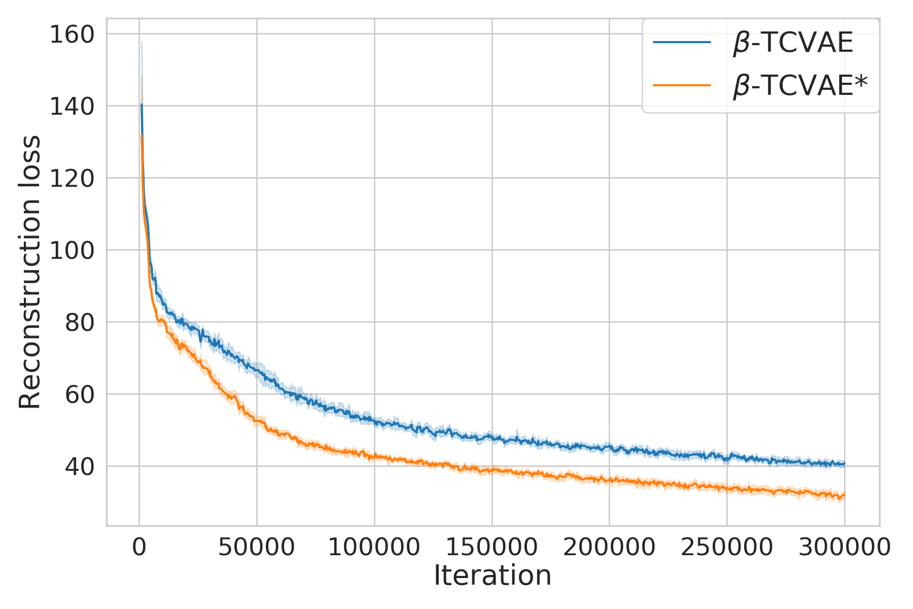
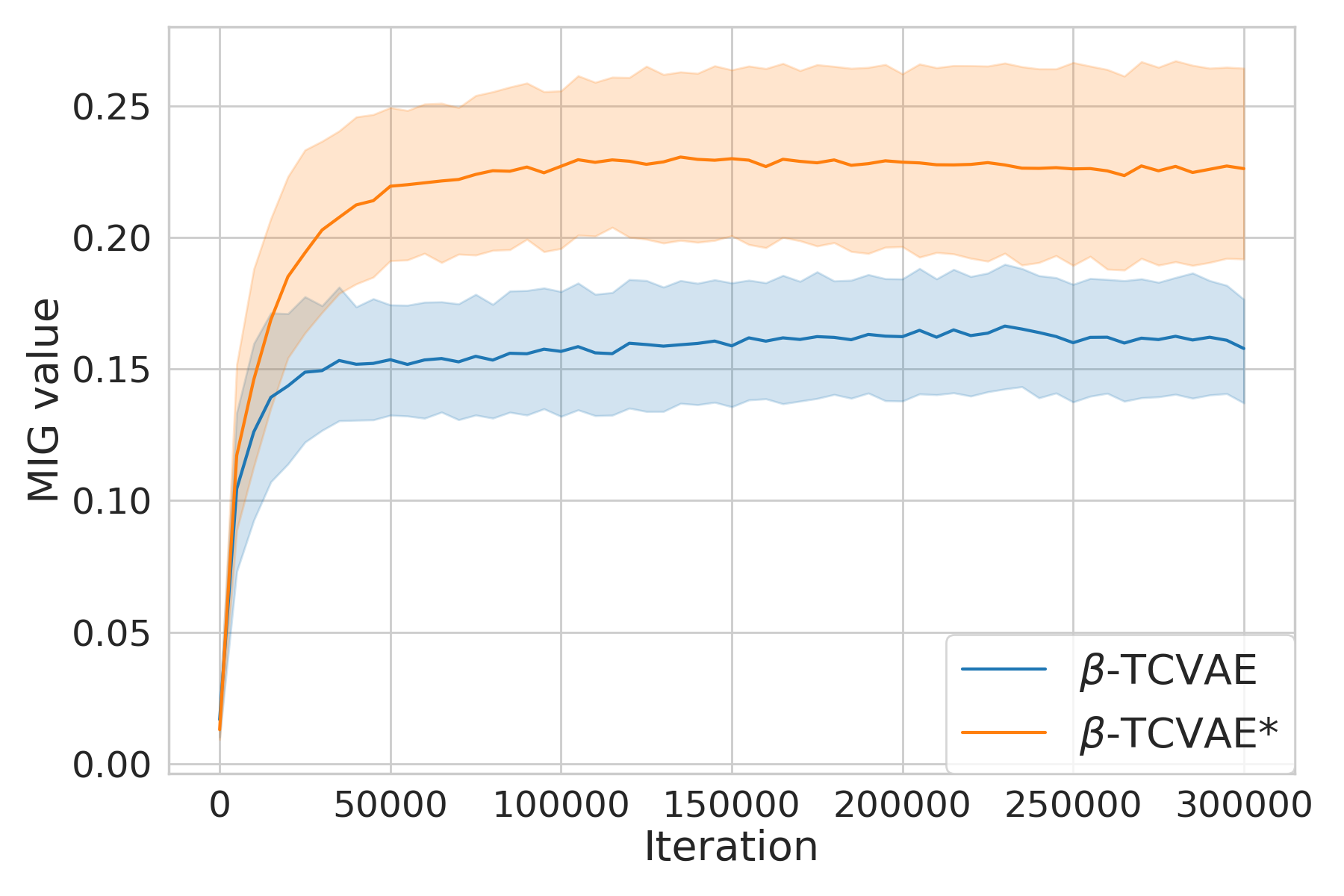
We compare β𝛽\beta-TCVAE with the original β𝛽\beta-TCVAE with the same value of β𝛽\beta. The comparison result on dSprites is shown in Fig. 9. It is interesting to find that β𝛽\beta-TCVAE is consistently better than classical β𝛽\beta-TCVAE in terms of both disentanglement and reconstruction.
Refer to caption
(a)
Refer to caption
(b)
Figure 9: The comparison of disentanglement (left) and reconstruction (right) between β𝛽\beta-TCVAE and β𝛽\beta-TCVAE on dSprites.

VI Related Work

VI-A Disentangled Representation Learning with VAEs

Before our work, many efforts have been made for disentangled representation learning with the VAE framework. In Section III-B we illustrate the connections between our PRI-VAE and some prevalent VAEs. More recently, HFVAE [9] decomposes the VAE objective into four terms, which provides a unified view to most VAE variants. Interested readers can refer to [30] for a comprehensive survey.

VI-B Interpreting DNNs with Information Theory

There has been a growing interest in understanding DNNs using information theory. According to [28], a DNN can be analyzed by measuring the amount of information that each hidden layer’s representation 𝐭𝐭\mathbf{t} preserves about the input signal 𝐱𝐱\mathbf{x} with respect to the desired response 𝐲𝐲\mathbf{y} (i.e., 𝐈(𝐱;𝐭)𝐈𝐱𝐭\mathbf{I}(\mathbf{x};\mathbf{t}) with respect to 𝐈(𝐭;𝐲)𝐈𝐭𝐲\mathbf{I}(\mathbf{t};\mathbf{y})). This technique has been applied to various DNN architectures, such as the the multilayer perceptrons (e.g., [6, 28]), the deterministic autoencoders (e.g., [33]) and the convolutional neural networks (e.g., [19, 35]). In general, most of these recent studies suggest that both 𝐈(𝐱;𝐭)𝐈𝐱𝐭\mathbf{I}(\mathbf{x};\mathbf{t}) and 𝐈(𝐭;𝐲)𝐈𝐭𝐲\mathbf{I}(\mathbf{t};\mathbf{y}) undergo separate “fitting” and “compression” phases, which is consistent with our observations as described in Section IV.

Before our work, [5] interpreted the emergence of disentangled representation in β𝛽\beta-VAE with the rate-distortion (RD) theorem [8, Chapter 10]. Similarly, [2] uses the RD function to explore the Pareto front of existing VAEs in terms of both rate (i.e., the average number of additional nats necessary to encode samples from the encoder) and distortion (i.e., the reconstruction error). On the other hand, [1] illuminates the connection between VAE and IB approach.

VII Conclusion

In this paper, we introduced the recently proposed matrix-based Rényi’s α𝛼\alpha-entropy functional to interpret the dynamics of learning of VAE models. We also developed a novel VAE learning objective and establish its connections to prior art. Extensive experimental results on four benchmark data sets suggest that our objective can obtain more interpretable factors and comparable disentangled representation while preserving a high reconstruction fidelity. Moreover, our objective can be easily tailored to expand its capacity; and the merit of our objective can be generalized to other SOTA models.

References

  • [1] A. Achille and S. Soatto, “Information dropout: Learning optimal representations through noisy computation,” IEEE Transactions on Pattern Analysis and Machine Intelligence, vol. 40, no. 12, pp. 2897–2905, 2018.
  • [2] A. Alemi, B. Poole, I. Fischer, J. Dillon, R. A. Saurous, and K. Murphy, “Fixing a broken elbo,” in International Conference on Machine Learning, 2018.
  • [3] M. Aubry, D. Maturana, A. A. Efros, B. C. Russell, and J. Sivic, “Seeing 3d chairs: exemplar part-based 2d-3d alignment using a large dataset of cad models,” in IEEE Conference on Computer Vision and Pattern Recognition, 2014.
  • [4] R. Bhatia, “Infinitely divisible matrices,” The American Mathematical Monthly, vol. 113, no. 3, pp. 221–235, 2006.
  • [5] C. P. Burgess, I. Higgins, A. Pal, L. Matthey, N. Watters, G. Desjardins, and A. Lerchner, “Understanding disentangling in β𝛽\beta-vae,” in Workshop on Learning Disentangled Representations at Neural Information Processing Systems, 2017.
  • [6] I. Chelombiev, C. Houghton, and C. O’Donnell, “Adaptive estimators show information compression in deep neural networks,” in International Conference on Learning Representations, 2018.
  • [7] T. Q. Chen, X. Li, R. B. Grosse, and D. K. Duvenaud, “Isolating sources of disentanglement in variational autoencoders,” in Advances in Neural Information Processing Systems, 2018.
  • [8] T. M. Cover and J. A. Thomas, Elements of information theory.   John Wiley & Sons, 2012.
  • [9] B. Esmaeili, H. Wu, S. Jain, A. Bozkurt, N. Siddharth, B. Paige, D. H. Brooks, J. Dy, and J.-W. Meent, “Structured disentangled representations,” in International Conference on Artificial Intelligence and Statistics, 2019.
  • [10] I. Higgins, L. Matthey, A. Pal, C. Burgess, X. Glorot, M. Botvinick, S. Mohamed, and A. Lerchner, “beta-vae: Learning basic visual concepts with a constrained variational framework.” in International Conference on Learning Representations, 2017.
  • [11] H. Kim and A. Mnih, “Disentangling by factorising,” in International Conference on Machine Learning, 2018.
  • [12] D. P. Kingma and M. Welling, “Auto-encoding variational bayes,” stat, vol. 1050, p. 10, 2014.
  • [13] A. Kraskov, H. Stögbauer, and P. Grassberger, “Estimating mutual information,” Physical review E, vol. 69, no. 6, p. 066138, 2004.
  • [14] A. Kumar, P. Sattigeri, and A. Balakrishnan, “Variational inference of disentangled latent concepts from unlabeled observations,” in International Conference on Learning Representations, 2018.
  • [15] J. Lezama, “Overcoming the disentanglement vs reconstruction trade-off via jacobian supervision,” in International Conference on Learning Representations, 2019.
  • [16] F. Locatello, S. Bauer, M. Lucic, G. Raetsch, S. Gelly, B. Schölkopf, and O. Bachem, “Challenging common assumptions in the unsupervised learning of disentangled representations,” in International Conference on Machine Learning, 2019.
  • [17] L. Matthey, I. Higgins, D. Hassabis, and A. Lerchner, “dsprites: Disentanglement testing sprites dataset,” https://github.com/deepmind/dsprites-dataset/, 2017.
  • [18] Y.-I. Moon, B. Rajagopalan, and U. Lall, “Estimation of mutual information using kernel density estimators,” Physical Review E, vol. 52, no. 3, p. 2318, 1995.
  • [19] M. Noshad, Y. Zeng, and A. O. Hero, “Scalable mutual information estimation using dependence graphs,” in IEEE International Conference on Acoustics, Speech and Signal Processing, 2019.
  • [20] L. Paninski, “Estimation of entropy and mutual information,” Neural Computation, vol. 15, no. 6, pp. 1191–1253, 2003.
  • [21] E. Parzen, “On estimation of a probability density function and mode,” The Annals of Mathematical Statistics, vol. 33, no. 3, pp. 1065–1076, 1962.
  • [22] J. C. Principe, Information theoretic learning: Renyi’s entropy and kernel perspectives.   Springer Science & Business Media, 2010.
  • [23] S. Rao, A. de Medeiros Martins, and J. C. Príncipe, “Mean shift: An information theoretic perspective,” Pattern Recognition Letters, vol. 30, no. 3, pp. 222–230, 2009.
  • [24] S. E. Reed, Y. Zhang, Y. Zhang, and H. Lee, “Deep visual analogy-making,” in Advances in Neural Information Processing Systems, 2015.
  • [25] A. Rényi, “On measures of entropy and information,” in Proceedings of the Fourth Berkeley Symposium on Mathematical Statistics and Probability, 1961.
  • [26] K. Ridgeway and M. C. Mozer, “Learning deep disentangled embeddings with the f-statistic loss,” in Advances in Neural Information Processing Systems, 2018.
  • [27] L. G. Sanchez Giraldo, M. Rao, and J. C. Principe, “Measures of entropy from data using infinitely divisible kernels,” IEEE Transactions on Information Theory, vol. 61, no. 1, pp. 535–548, 2014.
  • [28] R. Shwartz-Ziv and N. Tishby, “Opening the black box of deep neural networks via information,” arXiv preprint:1703.00810, 2017.
  • [29] N. Tishby, F. C. Pereira, and W. Bialek, “The information bottleneck method,” in Annual Allerton Conference on Communication, Control and Computing, 1999, pp. 368–377. [Online]. Available: https://arxiv.org/abs/physics/0004057
  • [30] M. Tschannen, O. Bachem, and M. Lucic, “Recent advances in autoencoder-based representation learning,” arXiv preprint:1812.05069, 2018.
  • [31] S. Watanabe, “Information theoretical analysis of multivariate correlation,” IBM Journal of research and development, vol. 4, no. 1, pp. 66–82, 1960.
  • [32] H. Xiao, K. Rasul, and R. Vollgraf, “Fashion-mnist: a novel image dataset for benchmarking machine learning algorithms,” arXiv preprint:1708.07747, 2017.
  • [33] S. Yu and J. C. Principe, “Understanding autoencoders with information theoretic concepts,” Neural Networks, vol. 117, pp. 104–123, 2019.
  • [34] S. Yu, L. G. Sanchez Giraldo, R. Jenssen, and J. C. Principe, “Multivariate extension of matrix-based renyi’s α𝛼\alpha-order entropy functional,” IEEE Transactions on Pattern Analysis and Machine Intelligence, 2019.
  • [35] S. Yu, K. Wickstrøm, R. Jenssen, and J. C. Principe, “Understanding convolutional neural networks with information theory: An initial exploration,” arXiv preprint:1804.06537, 2018.
  • [36] S. Zhao, J. Song, and S. Ermon, “Infovae: Balancing learning and inference in variational autoencoders,” in AAAI Conference on Artificial Intelligence, 2019.

Appendix A Proofs

A-A The Decomposition of DKL(qϕ(𝐳|𝐱)p(𝐳))subscript𝐷𝐾𝐿conditionalsubscript𝑞italic-ϕconditional𝐳𝐱𝑝𝐳D_{KL}(q_{\phi}(\mathbf{z}|\mathbf{x})\|p(\mathbf{z}))

Suppose the joint distribution of the data and the encoding distribution is given by q(𝐳,𝐱)=p(𝐱)qϕ(𝐳|𝐱)𝑞𝐳𝐱𝑝𝐱subscript𝑞italic-ϕconditional𝐳𝐱q(\mathbf{z},\mathbf{x})=p(\mathbf{x})q_{\phi}(\mathbf{z}|\mathbf{x}), the KL term DKL(qϕ(𝐳|𝐱)p(𝐳))subscript𝐷𝐾𝐿conditionalsubscript𝑞italic-ϕconditional𝐳𝐱𝑝𝐳D_{KL}(q_{\phi}(\mathbf{z}|\mathbf{x})\|p(\mathbf{z})) in the original VAE objective can be decomposed as follows [11].

𝔼p(𝐱)[DKL(qϕ(𝐳|𝐱)p(𝐳))]=𝔼p(𝐱)𝔼qϕ(𝐳|𝐱)[logqϕ(𝐳|𝐱)p(𝐳)]=𝔼q(𝐳,𝐱)[logqϕ(𝐳|𝐱)p(𝐳)q(𝐳)q(𝐳)]=𝔼q(𝐳,𝐱)[logqϕ(𝐳|𝐱)q(𝐳)]+𝔼q(𝐳,𝐱)[logq(𝐳)p(𝐳)]=𝔼q(𝐳,𝐱)[logq(𝐳,𝐱)q(𝐳)p(𝐱)]+𝔼q(𝐳)[logq(𝐳)p(𝐳)]=𝐈(𝐱;𝐳)+DKL(qϕ(𝐳)p(𝐳)).subscript𝔼𝑝𝐱delimited-[]subscript𝐷𝐾𝐿conditionalsubscript𝑞italic-ϕconditional𝐳𝐱𝑝𝐳subscript𝔼𝑝𝐱subscript𝔼subscript𝑞italic-ϕconditional𝐳𝐱delimited-[]subscript𝑞italic-ϕconditional𝐳𝐱𝑝𝐳subscript𝔼𝑞𝐳𝐱delimited-[]subscript𝑞italic-ϕconditional𝐳𝐱𝑝𝐳𝑞𝐳𝑞𝐳subscript𝔼𝑞𝐳𝐱delimited-[]subscript𝑞italic-ϕconditional𝐳𝐱𝑞𝐳subscript𝔼𝑞𝐳𝐱delimited-[]𝑞𝐳𝑝𝐳subscript𝔼𝑞𝐳𝐱delimited-[]𝑞𝐳𝐱𝑞𝐳𝑝𝐱subscript𝔼𝑞𝐳delimited-[]𝑞𝐳𝑝𝐳𝐈𝐱𝐳subscript𝐷𝐾𝐿conditionalsubscript𝑞italic-ϕ𝐳𝑝𝐳\begin{split}&\mathbb{E}_{p(\mathbf{x})}[D_{KL}(q_{\phi}(\mathbf{z}|\mathbf{x})\|p(\mathbf{z}))]\\ &=\mathbb{E}_{p(\mathbf{x})}\mathbb{E}_{q_{\phi}(\mathbf{z}|\mathbf{x})}[\log\frac{q_{\phi}(\mathbf{z}|\mathbf{x})}{p(\mathbf{z})}]\\ &=\mathbb{E}_{q(\mathbf{z},\mathbf{x})}[\log\frac{q_{\phi}(\mathbf{z}|\mathbf{x})}{p(\mathbf{z})}\frac{q(\mathbf{z})}{q(\mathbf{z})}]\\ &=\mathbb{E}_{q(\mathbf{z},\mathbf{x})}[\log\frac{q_{\phi}(\mathbf{z}|\mathbf{x})}{q(\mathbf{z})}]+\mathbb{E}_{q(\mathbf{z},\mathbf{x})}[\log\frac{q(\mathbf{z})}{p(\mathbf{z})}]\\ &=\mathbb{E}_{q(\mathbf{z},\mathbf{x})}[\log\frac{q(\mathbf{z},\mathbf{x})}{q(\mathbf{z})p(\mathbf{x})}]+\mathbb{E}_{q(\mathbf{z})}[\log\frac{q(\mathbf{z})}{p(\mathbf{z})}]\\ &=\mathbf{I}(\mathbf{x};\mathbf{z})+D_{KL}(q_{\phi}(\mathbf{z})\|p(\mathbf{z})).\end{split} (11)

Appendix B Experimental Details

B-A Information-Theoretic Quantities Estimation

Given input 𝐱p𝐱superscript𝑝\mathbf{x}\in\mathbb{R}^{p} and latent representation 𝐳d𝐳superscript𝑑\mathbf{z}\in\mathbb{R}^{d}, the standard Shannon (differential) entropy functional defines 𝐈(𝐱;𝐳)𝐈𝐱𝐳\mathbf{I}(\mathbf{x};\mathbf{z}) and 𝐓(𝐳)𝐓𝐳\mathbf{T}(\mathbf{z}) with Eq. (12) and Eq. (13), respectively:

𝐈(𝐱;𝐳)=DKL(p(𝐱,𝐳)p(𝐱)p(𝐳))=p(𝐱,𝐳)log(p(𝐱,𝐳)p(𝐱)p(𝐳))𝑑𝐱𝑑𝐳=𝐇(𝐱)+𝐇(𝐳)𝐇(𝐱,𝐳),𝐈𝐱𝐳subscript𝐷KLconditional𝑝𝐱𝐳𝑝𝐱𝑝𝐳𝑝𝐱𝐳𝑝𝐱𝐳𝑝𝐱𝑝𝐳differential-d𝐱differential-d𝐳𝐇𝐱𝐇𝐳𝐇𝐱𝐳\begin{split}\mathbf{I}(\mathbf{x};\mathbf{z})&=D_{\text{KL}}\left(p(\mathbf{x},\mathbf{z})\|p(\mathbf{x})p(\mathbf{z})\right)\\ &=\int\int p(\mathbf{x},\mathbf{z})\log\left(\frac{p(\mathbf{x},\mathbf{z})}{p(\mathbf{x})p(\mathbf{z})}\right)d\mathbf{x}d\mathbf{z}\\ &=\mathbf{H}(\mathbf{x})+\mathbf{H}(\mathbf{z})-\mathbf{H}(\mathbf{x},\mathbf{z}),\end{split} (12)
𝐓(𝐳)=DKL(p(𝐳)p(z1)p(zd))=p(𝐳)log(p(𝐳)p(z1)p(zd))𝑑z1𝑑zd=i=1d𝐇(zi)𝐇(𝐳),𝐓𝐳subscript𝐷KLconditional𝑝𝐳𝑝subscript𝑧1𝑝subscript𝑧𝑑𝑝𝐳𝑝𝐳𝑝subscript𝑧1𝑝subscript𝑧𝑑differential-dsubscript𝑧1differential-dsubscript𝑧𝑑superscriptsubscript𝑖1𝑑𝐇subscript𝑧𝑖𝐇𝐳\begin{split}\mathbf{T}(\mathbf{z})&=D_{\text{KL}}\left(p(\mathbf{z})\|p(z_{1})\cdots p(z_{d})\right)\\ &=\int\cdots\int p(\mathbf{z})\log\left(\frac{p(\mathbf{z})}{p(z_{1})\cdots p(z_{d})}\right)dz_{1}\cdots dz_{d}\\ &=\sum_{i=1}^{d}\mathbf{H}(z_{i})-\mathbf{H}(\mathbf{z}),\end{split} (13)

where 𝐇𝐇\mathbf{H} denotes the entropy of a single variable or joint entropy of multiple variables.

In the following of this section, we first give the novel definitions on the matrix-based Rényi’s α𝛼\alpha-order entropy and joint entropy, we then elaborate the implementation details in drawing the information plane of VAEs.

Definition 1

[27] Let κ:𝒳×𝒳:𝜅maps-to𝒳𝒳\kappa:\mathcal{X}\times\mathcal{X}\mapsto\mathbb{R} be a real valued positive definite kernel that is also infinitely divisible [4]. Given X={𝐱1,𝐱2,,𝐱N}𝑋superscript𝐱1superscript𝐱2superscript𝐱𝑁X=\{\mathbf{x}^{1},\mathbf{x}^{2},\cdots,\mathbf{x}^{N}\} and the Gram matrix K𝐾K obtained from evaluating a positive definite kernel κ𝜅\kappa on all pairs of exemplars, that is (K)ij=κ(𝐱i,𝐱j)subscript𝐾𝑖𝑗𝜅superscript𝐱𝑖superscript𝐱𝑗(K)_{ij}=\kappa(\mathbf{x}^{i},\mathbf{x}^{j}), a matrix-based analogue to Rényi’s α𝛼\alpha-entropy for a normalized positive definite (NPD) matrix A𝐴A of size n×n𝑛𝑛n\times n, such that tr(A)=1tr𝐴1\mathrm{tr}(A)=1, can be given by the following functional:

𝐒α(A)=11αlog2(tr(Aα))=11αlog2[i=1Nλi(A)α]subscript𝐒𝛼𝐴11𝛼subscript2trsuperscript𝐴𝛼11𝛼subscript2superscriptsubscript𝑖1𝑁subscript𝜆𝑖superscript𝐴𝛼\mathbf{S}_{\alpha}(A)=\frac{1}{1-\alpha}\log_{2}\left(\mathrm{tr}(A^{\alpha})\right)=\frac{1}{1-\alpha}\log_{2}\big{[}\sum_{i=1}^{N}\lambda_{i}(A)^{\alpha}\big{]} (14)

where Aij=1NKijKiiKjjsubscript𝐴𝑖𝑗1𝑁subscript𝐾𝑖𝑗subscript𝐾𝑖𝑖subscript𝐾𝑗𝑗A_{ij}=\frac{1}{N}\frac{K_{ij}}{\sqrt{K_{ii}K_{jj}}} and λi(A)subscript𝜆𝑖𝐴\lambda_{i}(A) denotes the i𝑖i-th eigenvalue of A𝐴A.

Definition 2

[34] Given a collection of N𝑁N samples {si=(𝐱1i,𝐱2i,,𝐱di)}i=1Nsuperscriptsubscriptsubscript𝑠𝑖superscriptsubscript𝐱1𝑖superscriptsubscript𝐱2𝑖superscriptsubscript𝐱𝑑𝑖𝑖1𝑁\{s_{i}=(\mathbf{x}_{1}^{i},\mathbf{x}_{2}^{i},\cdots,\mathbf{x}_{d}^{i})\}_{i=1}^{N}, where the superscript i𝑖i denotes the sample index, each sample contains d𝑑d (d2𝑑2d\geq 2) measurements 𝐱1𝒳1subscript𝐱1subscript𝒳1\mathbf{x}_{1}\in\mathcal{X}_{1}, 𝐱2𝒳2subscript𝐱2subscript𝒳2\mathbf{x}_{2}\in\mathcal{X}_{2}, \cdots, 𝐱d𝒳dsubscript𝐱𝑑subscript𝒳𝑑\mathbf{x}_{d}\in\mathcal{X}_{d} obtained from the same realization, and the positive definite kernels κ1:𝒳1×𝒳1:subscript𝜅1maps-tosubscript𝒳1subscript𝒳1\kappa_{1}:\mathcal{X}_{1}\times\mathcal{X}_{1}\mapsto\mathbb{R}, κ2:𝒳2×𝒳2:subscript𝜅2maps-tosubscript𝒳2subscript𝒳2\kappa_{2}:\mathcal{X}_{2}\times\mathcal{X}_{2}\mapsto\mathbb{R}, \cdots, κd:𝒳d×𝒳d:subscript𝜅𝑑maps-tosubscript𝒳𝑑subscript𝒳𝑑\kappa_{d}:\mathcal{X}_{d}\times\mathcal{X}_{d}\mapsto\mathbb{R}, a matrix-based analogue to Rényi’s α𝛼\alpha-order joint-entropy among d𝑑d variables can be defined as:

𝐒α(A1,A2,,Ad)=𝐒α(A1A2Adtr(A1A2Ad))subscript𝐒𝛼subscript𝐴1subscript𝐴2subscript𝐴𝑑subscript𝐒𝛼subscript𝐴1subscript𝐴2subscript𝐴𝑑trsubscript𝐴1subscript𝐴2subscript𝐴𝑑\mathbf{S}_{\alpha}(A_{1},A_{2},\cdots,A_{d})=\mathbf{S}_{\alpha}\left(\frac{A_{1}\circ A_{2}\circ\cdots\circ A_{d}}{\mathrm{tr}(A_{1}\circ A_{2}\circ\cdots\circ A_{d})}\right) (15)

where (A1)ij=κ1(𝐱1i,𝐱1j)subscriptsubscript𝐴1𝑖𝑗subscript𝜅1superscriptsubscript𝐱1𝑖superscriptsubscript𝐱1𝑗(A_{1})_{ij}=\kappa_{1}(\mathbf{x}_{1}^{i},\mathbf{x}_{1}^{j}), (A2)ij=κ2(𝐱2i,𝐱2j)subscriptsubscript𝐴2𝑖𝑗subscript𝜅2superscriptsubscript𝐱2𝑖superscriptsubscript𝐱2𝑗(A_{2})_{ij}=\kappa_{2}(\mathbf{x}_{2}^{i},\mathbf{x}_{2}^{j}), \cdots, (Ad)ij=κd(𝐱di,𝐱dj)subscriptsubscript𝐴𝑑𝑖𝑗subscript𝜅𝑑superscriptsubscript𝐱𝑑𝑖superscriptsubscript𝐱𝑑𝑗(A_{d})_{ij}=\kappa_{d}(\mathbf{x}_{d}^{i},\mathbf{x}_{d}^{j}), and \circ denotes the Hadamard product.

We use RBF kernel as recommended by [35], and estimate 𝐈(𝐱;𝐳)𝐈𝐱𝐳\mathbf{I}(\mathbf{x};\mathbf{z}) and 𝐓(𝐳)𝐓𝐳\mathbf{T}(\mathbf{z}) in each training iteration. Given input data in current mini-batch (of size N𝑁N) X={𝐱1,𝐱2,,𝐱N}𝑋superscript𝐱1superscript𝐱2superscript𝐱𝑁X=\{\mathbf{x}^{1},\mathbf{x}^{2},\cdots,\mathbf{x}^{N}\}, suppose the corresponding latent representation is Z={𝐳1,𝐳2,,𝐳N}𝑍superscript𝐳1superscript𝐳2superscript𝐳𝑁Z=\{\mathbf{z}^{1},\mathbf{z}^{2},\cdots,\mathbf{z}^{N}\}, in which 𝐳i=[z1i,z2i,,zdi]Tsuperscript𝐳𝑖superscriptsubscriptsuperscript𝑧𝑖1subscriptsuperscript𝑧𝑖2subscriptsuperscript𝑧𝑖𝑑𝑇\mathbf{z}^{i}=[z^{i}_{1},z^{i}_{2},\cdots,z^{i}_{d}]^{T}. Both 𝐈(𝐱;𝐳)=𝐇(𝐱)+𝐇(𝐳)𝐇(𝐱,𝐳)𝐈𝐱𝐳𝐇𝐱𝐇𝐳𝐇𝐱𝐳\mathbf{I}(\mathbf{x};\mathbf{z})=\mathbf{H}(\mathbf{x})+\mathbf{H}(\mathbf{z})-\mathbf{H}(\mathbf{x},\mathbf{z}) and 𝐓(𝐳)=i=1d𝐇(zi)𝐇(𝐳)𝐓𝐳superscriptsubscript𝑖1𝑑𝐇subscript𝑧𝑖𝐇𝐳\mathbf{T}(\mathbf{z})=\sum_{i=1}^{d}\mathbf{H}(z_{i})-\mathbf{H}(\mathbf{z}) can be simply evaluated based on Definition 1 and Definition 2.

For example, in order to estimate 𝐇(𝐳)𝐇𝐳\mathbf{H}(\mathbf{z}), one just needs to compute a N×N𝑁𝑁N\times N Gram matrix A𝐴A in which A(i,j)𝐴𝑖𝑗A(i,j) measures the distance between latent representation 𝐳isubscript𝐳𝑖\mathbf{z}_{i} (of the i𝑖i-th mini-batch sample) and 𝐳jsubscript𝐳𝑗\mathbf{z}_{j} (of the j𝑗j-th mini-batch sample) in the kernel space. Since the new estimator involves eigenvalue decomposition to matrices of N×N𝑁𝑁N\times N, the scalability depends on the mini-batch size. Luckily, state-of-the-art VAEs are always trained with N𝑁N equal to 646464.

Finally, in order to obtain a smoother visualization on the information plane, we sample 6,40064006,400 data points and obtain the latent representation by feeding them into the Gaussian type encoder. We then use the matrix-based Rényi’s α𝛼\alpha-entropy functional to compute 𝐈(𝐱;𝐳)𝐈𝐱𝐳\mathbf{I}(\mathbf{x};\mathbf{z}) and 𝐓(𝐳)𝐓𝐳\mathbf{T}(\mathbf{z}) in a mini-batch of size 646464 to obtain 100100100 estimation values to both quantities. We finally average the 100100100 estimation values to obtain a stable result.

TABLE B1: The unified network architecture in Section 6.1 experiments.
Encoder Decoder
FC, 2×102102\times 10 (mean, log variance) Input: 10superscript10\mathbb{R}^{10}
FC, 256 ReLU FC, 256 ReLU
4×4444\times 4 Conv, stride 2, 64 ReLU FC, 4×4×6444644\times 4\times 64 ReLU
4×4444\times 4 Conv, stride 2, 64 ReLU 4×4444\times 4 Upconv, stride 2, 64 ReLU
4×4444\times 4 Conv, stride 2, 32 ReLU 4×4444\times 4 Upconv, stride 2, 32 ReLU
Input: 64×64×64\times 64\times #channel 4×4444\times 4 Upconv, stride 2, #channel
TABLE B2: The network architecture for the discriminator in FactorVAE.
Discriminator
FC, 1000 leaky ReLU
FC, 1000 leaky ReLU
FC, 1000 leaky ReLU
FC, 1000 leaky ReLU
FC, 1000 leaky ReLU
FC, 1000 leaky ReLU
FC, 2

B-B Quantitative Evaluation

In the quantitative comparison experiments, we use a unified network architecture, which is shown in the Table B1. A Gaussian type encoder outputs the mean and the log variance given the image data, and a Bernoulli type decoder takes the mean as the input and outputs the generated images. The models are optimized by the Adam optimiser with learning rate 1×1041E-41\text{\times}{10}^{-4}, β1=0.9subscript𝛽10.9\beta_{1}=0.9, β2=0.999subscript𝛽20.999\beta_{2}=0.999, the batch size is fixed as 646464 and the total training steps are 300 000300000300\,000 for both of dSprites and Cars3D data sets. Table B2 lists the discriminator architecture for FactorVAE, and we use the Adam optimiser with learning rate 1×1041E-41\text{\times}{10}^{-4}, β1=0.5subscript𝛽10.5\beta_{1}=0.5, β2=0.9subscript𝛽20.9\beta_{2}=0.9, ϵ=1×10⁸italic-ϵ1E-8\epsilon=$1\text{\times}{10}^{-8}$ for optimization.

B-C Qualitative Evaluation

Table B3 shows the network architecture used in the Section 6.2 for qualitative evaluation on 3D Chairs and Fashion-MNIST data sets. The following sections list the training details respectively.

TABLE B3: The network architecture in Section 6.2 experiments.
Encoder Decoder
FC, 2×102102\times 10 (mean, log variance) Input: 10superscript10\mathbb{R}^{10}
2FCs, 256 ReLU 2FCs, 256 ReLU
4×4444\times 4 Conv, stride 2, 32 ReLU FC, 4×4×3244324\times 4\times 32 ReLU
4×4444\times 4 Conv, stride 2, 32 ReLU 4×4444\times 4 Upconv, stride 2, 32 ReLU
Input: 64×64×64\times 64\times #channel 4×4444\times 4 Upconv, stride 2, #channel

B-C1 3D Chairs

  • Decoder type: Bernoulli

  • Batch size: 64

  • Training epochs: 300

  • Optimizer: Adam with learning rate 1×1041E-41\text{\times}{10}^{-4}

B-C2 Fashion-MNIST

  • Decoder type: Bernoulli

  • Batch size: 64

  • Training epochs: 400

  • Optimizer: Adam with learning rate 1×1041E-41\text{\times}{10}^{-4}

Appendix C Additional Results

C-A Empirical behavior of 𝐈(𝐱;𝐳)𝐈𝐱𝐳\mathbf{I}(\mathbf{x};\mathbf{z}) and 𝐓(𝐳)𝐓𝐳\mathbf{T}(\mathbf{z})

The matrix-based Rényi’s α𝛼\alpha-entropy introduces a hyper-parameter α𝛼\alpha when estimating the entropy value of the input. To verify the consistency of the observed general trend of dynamic of learning presented in Section IV and reduce the possible effects introduces by different hyper-parameter setting, we demonstrate the empirical behavior of 𝐈(𝐱;𝐳)𝐈𝐱𝐳\mathbf{I}(\mathbf{x};\mathbf{z}) and 𝐓(𝐳)𝐓𝐳\mathbf{T}(\mathbf{z}) with additional α𝛼\alpha setting for matrix-based Rényi’s α𝛼\alpha-entropy estimator. Fig. C1 and Fig. C2 illustrate observation results with α=2.0𝛼2.0\alpha=2.0 and α=0.6𝛼0.6\alpha=0.6 respectively. We can find that our general observation is accordance with different hyper-parameter settings.
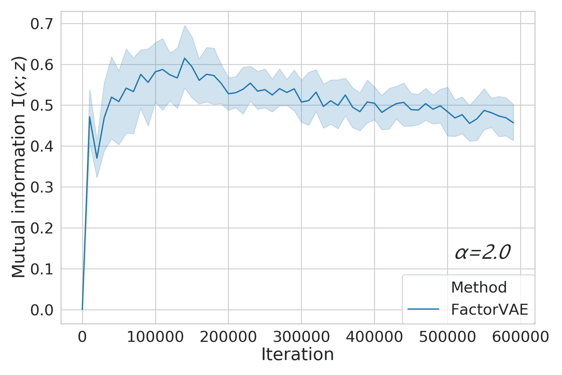
Refer to caption
(a)
Refer to caption
(b)
Refer to caption
(c)
Refer to caption
(d)
Refer to caption
(e)
Refer to caption
(f)
Refer to caption
(g)
Refer to caption
(h)
Refer to caption
(i)
Figure C1: Measured by the matrix-based Rényi’s α𝛼\alpha-entropy estimator with α=2.0𝛼2.0\alpha=2.0, the evolution of the value of 𝐈(𝐱;𝐳)𝐈𝐱𝐳\mathbf{I}(\mathbf{x};\mathbf{z}) (left column) and the value of 𝐓(𝐳)𝐓𝐳\mathbf{T}(\mathbf{z}) (middle column) across training iterations for FactorVAE (first row), β𝛽\beta-TCVAE (second row) and PRI-VAE (third row) on Cars3d data set. The right column shows the positive correlation between these two values.
Refer to caption
(a)
Refer to caption
(b)
Refer to caption
(c)
Refer to caption
(d)
Refer to caption
(e)
Refer to caption
(f)
Refer to caption
(g)
Refer to caption
(h)
Refer to caption
(i)
Figure C2: Measured by the matrix-based Rényi’s α𝛼\alpha-entropy estimator with α=0.6𝛼0.6\alpha=0.6, the evolution of the value of 𝐈(𝐱;𝐳)𝐈𝐱𝐳\mathbf{I}(\mathbf{x};\mathbf{z}) (left column) and the value of 𝐓(𝐳)𝐓𝐳\mathbf{T}(\mathbf{z}) (middle column) across training iterations for FactorVAE and β𝛽\beta-TCVAE on Cars3d data set. The right column shows the positive correlation between these two values.

C-B DCI disentanglement metric

Fig. C3 demonstrates the DCI disentanglement metric score for PRI-VAE and all other competing models in dSprites and Cars3D. It shows the similar comparison results as illustrated and discussed in Section V-A2, where PRI-VAE achieves consistent better disentanglement performance than VAE, β𝛽\beta-VAE, AnnealedVAE, and DPI-VAE, but worse performance than FactorVAE and β𝛽\beta-TCVAE.

Refer to caption
(a)
Refer to caption
(b)
Figure C3: The DCI disentanglement metric on dSprites (left) and Cars3D (right) data sets.

Table C4 shows the DCI disentanglement scores of β𝛽\beta-TCVAE, PRI-VAE and PRI-VAE on dSprites and Cars3D. Similar comparison results are obtained and discussed in Section V-A2.

TABLE C4: The DCI disentanglement scores of β𝛽\beta-TCVAE, PRI-VAE and PRI-VAE on dSprites and Cars3D. We report the mean value over 101010 runs and the standard deviation in parentheses.
β𝛽\beta-TCVAE PRI-VAE PRI-VAE
dSprites 0.318 (0.040) 0.234 (0.058) 0.345 (0.088)
Cars3D 0.343 (0.037) 0.281 (0.050) 0.321 (0.048)

C-C Hyper-parameter Analysis

Fig. C4 shows the MIG score and the reconstruction loss measured at the end of training with respect to different values of β𝛽\beta and α=1𝛼1\alpha=1 in dSprites data set. Obviously, with the increase of β𝛽\beta, the model disentanglement performance increases accordingly. This makes sense, because we penalize more on the independence between each dimension of z𝑧z. However, we also observed an obvious trade-off before disentanglement and reconstruction, which has also been mentioned in previous works (e.g., [11, 7]). We intend to address this problem in the future. A promising solution comes from [15].

On the other hand, it is worth noting that our model is hard to convergence when α>β𝛼𝛽\alpha>\beta. This result matches well with the property of PRI. As discussed earlier, β/α𝛽𝛼\beta/\alpha plays the same role as γ𝛾\gamma in PRI. Theoretically, PRI with γ=1𝛾1\gamma=1 reduces to the classical mean shift algorithm [23] such that it will iteratively reaching to the mode of the prior distribution. Note that, the mode of an isotropic Gaussian is exactly its mean vector (a single point in latent space). Therefore, β/α=1𝛽𝛼1\beta/\alpha=1 pushes our latent representation to a single point. Obviously, this will seriously impedes our training. In fact, as demonstrated in Fig. 1 in the main text, β/α2𝛽𝛼2\beta/\alpha\geq 2 is able to balance a good trade-off between structure preservation and uncertainty filtering. Therefore, we recommend β2α𝛽2𝛼\beta\geq 2\alpha.

In this section, we investigate the effects of hyper-parameters α𝛼\alpha and β𝛽\beta to the performance of PRI-VAE.

Refer to caption
Figure C4: The disentanglement and reconstruction trade-off with respect to different parameter setting of α𝛼\alpha and β𝛽\beta in PRI-VAE. When α>β𝛼𝛽\alpha>\beta, the model does not converge.

C-D More Qualitative Results

Refer to caption
(a) The reconstruction results of PRI-VAE on dsprites data set.
Refer to caption
(b) The reconstruction results of PRI-VAE on cars3d data set.
Figure C5: The reconstruction results of PRI-VAE model on (a) dsprites and (b) cars3d data sets. The odd columns represents the input data point and even columns are their reconstructions. PRI-VAE encourages more disentangled representations and reasonable reconstruction quality.